cost-effective fuel choices in the transportation sector
TRANSCRIPT

THESIS FOR THE DEGREE OF LICENTIATE IN ENVIRONMENTAL SCIENCE
Cost-effective fuel choices in the transportation sector under stringent CO2-emission reduction targets
Global energy systems modelling
MARIA GRAHN
Physical Resource Theory Department of Energy and Environment
Chalmers University of Technology Göteborg, Sweden 2006

Cost-effective fuel choices in the transportation sector under stringent CO2-emission reduction targets – Global energy systems modelling Maria Grahn © Maria Grahn, 2006 Physical Resource Theory Department of Energy and Environment Chalmers University of Technology SE-412 96 Göteborg Sweden Telephone: +46 (0)31-772 10 00 Email: [email protected] URL: www.frt.fy.chalmers.se Printed by Chalmers Reproservice Göteborg, Sweden 2006

i
Cost-effective fuel choices in the transportation sector under stringent CO2-emission reduction targets
Maria Grahn
Physical Resource Theory, Department of Energy and Environment,
Chalmers University of Technology, 2006
Abstract This thesis analyzes the world’s future energy supply in general, and cost-effective fuel choices in
the transportation sector in particular, under stringent CO2 constraints. The analysis is carried out
with the help of a global energy systems model (GET), developed and modified specifically for
each project. GET is a linear programming model and it has three end-use sectors: electricity,
heat and transportation fuel. It is set up to generate the energy supply mix that would meet
exogenously given energy demand levels at the lowest global cost. This thesis consists of the
following three papers (i) an analysis of why two similar global energy systems models, GET and
BEAP, give different results as to whether biofuels will become cost-effective in the
transportation sector, (ii) an analysis of cost effective fuel choices in a regionalized version of the
GET model and (iii) an analysis of the cost dynamics in the GET model in a further developed
version of the model. Conclusions drawn within the scope of this thesis are that biomass is most
cost-effectively used for heat production at low CO2 taxes, up to about 75 USD/tC, as shown in
both the GET and the BEAP model. The sector in which biomass is most cost-effectively used at
higher CO2 taxes depends on assumed possible energy carriers and technologies. If hydrogen
and/or electricity derived from carbon free energy sources will not be available in the
transportation sector at sufficiently low costs, biofuels become an important option if low or zero
carbon emissions are to be achieved. Thus, the long run future for the cost-effective transportation
fuel choice is still in the open. Regionalizing the GET 1.0 model will not affect the overall pattern
of transportation fuel choices, i.e. that gasoline/diesel remain for some decades in the
transportation sector until the carbon constraint becomes increasingly stringent and that solar
based hydrogen dominates by the end of this century. In paper III, we find that the required
carbon tax level where biofuels become cost-efficient, compared to fossil based fuels, is evasive.
The tax level moves upwards with increasing carbon taxes, since this leads to an increasing
biomass primary energy price in the model.
Keywords: Global energy systems, energy scenarios, transportation sector, carbon dioxide
emissions, biomass, liquid biofuels, hydrogen, carbon tax, primary energy price

ii

iii
List of publications This thesis is based on the following appended publications:
I. Biomass for heat or as transportation fuel? – a comparison between two
model based studies
Grahn M, C Azar, K Lindgren, G Berndes and D Gielen, 2005.
Submitted for publication in Biomass and Bioenergy.
II. Regionalized global energy scenarios meeting stringent climate targets –
cost effective fuel choices in the transportation sector
Grahn M, C. Azar and K. Lindgren. Conference proceedings.
Risö International Energy Conference, 19-21 May, 2003.
To be submitted.
III. Biomass for heat or transport – an exploration into the underlying cost
dynamics in the GET model
Grahn M, K. Lindgren and C. Azar, 2006.
Working paper. To be submitted.

iv

1
Table of contents 1. INTRODUCTION .................................................................................................................................... 3
1.1 ALTERNATIVE TRANSPORTATION FUELS ............................................................................................... 8 1.2 COST-EFFICIENT FUEL CHOICES MEETING AMBITIOUS CLIMATIC TARGETS – RESULTS FROM PREVIOUS GET MODEL STUDIES ............................................................................................................................... 11 1.3 MY RESEARCH .................................................................................................................................... 13
2. METHOD................................................................................................................................................ 14 2.1 MODEL STRUCTURE ............................................................................................................................ 15 2.2 ENERGY DEMAND SCENARIOS............................................................................................................. 16 2.3 CONSTRAINTS AND ASSUMPTIONS ...................................................................................................... 16
3. RESEARCH STUDIES.......................................................................................................................... 17 3.1 PAPER I: BIOMASS FOR HEAT OR AS TRANSPORTATION FUEL? – A COMPARISON BETWEEN TWO MODEL BASED STUDIES......................................................................................................................................... 17
3.1.1 Background and research question............................................................................................ 17 3.1.2 Method ....................................................................................................................................... 18 3.1.3 Main results ............................................................................................................................... 20
3.2 PAPER II: REGIONALIZATION OF THE GET MODEL.............................................................................. 22 3.2.1 Background and research question............................................................................................ 22 3.2.2 Method ....................................................................................................................................... 23 3.2.3 Main results ............................................................................................................................... 24 3.2.4 Future work................................................................................................................................ 27
3.3 PAPER III: BIOMASS FOR HEAT OR TRANSPORT – AN EXPLORATION INTO THE UNDERLYING COST DYNAMICS IN THE GET MODEL ................................................................................................................ 28
3.3.1 Background and research question............................................................................................ 28 3.3.2 Method ....................................................................................................................................... 28 3.3.3 Main results ............................................................................................................................... 30
4. EXPLAINING THE MODEL RESULTS ............................................................................................ 36 4.1 HOW CAN OIL REMAIN DOMINANT IN THE TRANSPORTATION SECTOR FOR SEVERAL DECADES DESPITE THE INTRODUCTION OF STRINGENT CLIMATE TARGETS? ........................................................................... 36
4.1.1 A physical explanation ............................................................................................................... 37 4.1.2 Energy conversion efficiency ..................................................................................................... 37
4.2 WHY ARE NOT BIOFUELS SEEN AS A COST-EFFECTIVE STRATEGY TO REDUCE CO2 EMISSIONS? .......... 38 5. DISCUSSION.......................................................................................................................................... 39
5.1 FACTORS NOT CONSIDERED IN THE GET MODEL................................................................................. 39 5.1.1 Surplus of cropland.................................................................................................................... 40 5.1.2 Energy security .......................................................................................................................... 41 5.1.3 Barriers for biomass in the heat sector...................................................................................... 41
5.2 IS IT REASONABLE TO ASSUME THAT CO2-NEUTRAL HYDROGEN WILL OVERCOME ITS BARRIERS AND BE AVAILABLE IN THE TRANSPORTATION SECTOR?........................................................................................ 41
6. CONCLUSIONS..................................................................................................................................... 42 7. SOME IMPLICATIONS FOR POLICY ............................................................................................. 44
7.1 POLICY INSTRUMENTS FOR THE TRANSPORTATION SECTOR ................................................................ 44 7.2 BRING DOWN COSTS FOR ALL PROMISING CO2-NEUTRAL OPTIONS ..................................................... 45 7.3 POLICY INSTRUMENTS FOR THE ENERGY SYSTEM ............................................................................... 45
ACKNOWLEDGEMENT ......................................................................................................................... 46 REFERENCES ........................................................................................................................................... 50

2

3
1. Introduction Science is not and will never be static final knowledge. To explain nature we are using
models and these models are further developed as soon as we get more information. A
famous example of such continuously developed model is the model describing the
movements within our solar system. The early Ptolemy’s geocentric model, which
assumed the earth at rest in the centre of universe with the rest of the planets revolving
around it, was in 1543 replaced by Copernicus’ heliocentric model in which the planets
revolve around a fixed sun. The model was then further developed by Tycho Brahe,
Johannes Kepler, Galileo Galilei and others into the model which we use today, based on
physical laws described by Isaac Newton and Albert Einstein, where the sun is at the
centre of our solar system, which is moving in the Milky Way galaxy which is moving in
the universe. Science always reflects current knowledge and as far as we know today we
are phasing the start of a climatic change.
By studying ice cores and actual measurements we can observe a dramatic increase in
the concentration of carbon dioxide in the atmosphere since the year 1750, see Figure 1.
Figure 1. Atmospheric carbon dioxide concentration during the last millennium. The pre-industrial level
was around 280 ppm and currently the concentration is 370 ppm. Source: IPCC (2001a).
There is complete consensus among scientists that carbon dioxide is a gas that absorbs
and emits long-wave radiation. Thus, the higher the concentration of atmospheric carbon

4
dioxide molecules, the more heat can be absorbed. The physics of the greenhouse effect1,
and the role of atmospheric carbon dioxide, have reached high levels of scientific
understanding and it is now understood that the greenhouse effect depends on two
factors: the difference between surface and atmospheric temperatures, and the
atmospheric emissivity2. The greenhouse effect increases as either of these terms
increases (Harvey, 2000). How sensitive the global climate is to the increase of
greenhouse gases and how sensitive plants and animals are to a temperature rise are
however questions to be further studied.
The Intergovernmental Panel on Climate Change (IPCC) has summarized current
knowledge on the global annual average surface temperature, which may evolve under
various CO2 emission paths for various stabilization scenarios, see Figure 2.
Figure 2. a) Different CO2 emission reduction paths corresponding to various stabilization concentrations
of atmospheric CO2 and b) assumed increase in global annual average surface temperatures, from the base
period 1961-1990 average, with corresponding uncertainty bars. Source: IPCC (2001a)
1 The term greenhouse effect refers to the reduction in outgoing heat radiation to space due to the presence of atmosphere (Harvey, 2000). The natural greenhouse effect is necessary for the life on earth as we know it, since the surface temperature is about 30 oC higher than if the planet had been without a natural greenhouse effect (NE, 2005). 2 All objects above absolute zero (-273 oC) emit electromagnetic radiation. Objects that emit the maximum amount of radiation are called blackbodies and the ratio of actual emission to blackbody emission is called the emissivity. The atmospheric emissivity depends on the concentration of gases such as CO2 (Harvey, 2000).

5
The most ambitious carbon dioxide stabilization target, presented in Figure 2, is a
450 ppm scenario corresponding to approximately 1.5-3 oC 3 increase in global mean
temperature above the base period 1961-1990 average and the least ambitious
stabilization target is a 1000 ppm scenario corresponding to approximately 3-6.5 oC 4
increase in global mean temperature above the 1961-1990 average. To put these
1.5-6.5 oC in a broader perspective it can be noted that the global average surface
temperature has increased over the 20th century by 0.6 oC and we can observe for
example that snow cover and ice extent have decreased, that the global average sea level
has risen and that precipitation patterns have changed (IPCC, 2001b). It can also be
noted that there have been glacial periods on earth at approximately 5 oC lower mean
temperature. Currently, large uncertainties remain on what will happen at a global mean
temperature increase of 1.5-6.5 oC.
Defining what CO2 concentration level that avoids “dangerous anthropogenic
interference” with the climate system, remains a challenge. However, O’Neill and
Oppenheimer (2002) argue that stabilizing the CO2 concentrations near 450 ppm would
likely preserve the option of avoiding shutdown of the density driven, large-scale
thermohaline circulation of the oceans, e.g. the Gulf Stream, and may also forestall the
disintegration of the West Antarctic Ice Sheet. However, such a target appears to be
inadequate for preventing severe damage to some coral reef systems. Further Azar and
Rodhe (1997) suggest that a temperature increase by 2 oC above pre-industrial levels may
be seen as a critical level and that the global community should initiate policies that make
stabilization in the range 350-400 ppm possible, to avoid reaching this critical level. The
European Council has agreed on a climate target that the global annual mean surface
temperature increase should not exceed 2 ºC above pre-industrial levels (European
Council, 2005).
3 Also 1.5-4 oC above pre-industrial levels are found in literature (Azar&Rodhe, 1997). 4 Also 3-9 oC above pre-industrial levels are found in literature (Azar&Rodhe, 1997).

6
To stabilize the CO2 concentrations near 450 ppm, Figure 1 indicate that the yearly global
CO2 emissions need to come down to about 2 GtC (2 billion ton carbon) within this
century.
For the sake of illustrating the scale of the challenge, we do the following exercise:
Assuming a future population of 10 billion people, the global average per capita
emissions must decrease to 0.2 tC/yr, see the dotted line in Figure 3. This is less than
what the lowest CO2-emitting regions e.g. India and Africa emits per capita today.
Reducing the global CO2 emission down to 2 GtC/yr is a huge challenge.
-
1.00
2.00
3.00
4.00
5.00
6.00
0 1,000 2,000 3,000 4,000 5,000 6,000Population (million)
Emis
sion
s (to
n ca
rbon
per
cap
ita)
USA
Canada, Australia, New Zealand
JapanOECD Europe
Russia
Other Europe
China
Middle East
IndiaOther Asia Africa
Latin AmericaWorld Average
-
1.00
2.00
3.00
4.00
5.00
6.00
0 1,000 2,000 3,000 4,000 5,000 6,000Population (million)
Emis
sion
s (to
n ca
rbon
per
cap
ita)
USA
Canada, Australia, New Zealand
JapanOECD Europe
Russia
Other Europe
China
Middle East
IndiaOther Asia Africa
Latin AmericaWorld Average
-
1.00
2.00
3.00
4.00
5.00
6.00
0 1,000 2,000 3,000 4,000 5,000 6,000Population (million)
Emis
sion
s (to
n ca
rbon
per
cap
ita)
USA
Canada, Australia, New Zealand
JapanOECD Europe
Russia
Other Europe
China
Middle East
IndiaOther Asia Africa
Latin AmericaWorld Average
Figure 3. CO2 emissions in ton carbon per capita, year 1998, for different regions (data from Marland et
al., 2002). To meet the global goal of 2 GtC CO2 emission per year, every country needs to reduce their
CO2 emissions per capita down to 0.2 tC/yr, by the year 2100. This per capita goal is marked with a dotted
line, in the figure.
The major source, of anthropogenic CO2 emissions, is the combustion of fossil fuels and
a large transition of the global energy system is necessary to be able to reach ambitious
CO2 stabilization levels. Two of the three studies appended to this thesis analyses how
the energy system can be transformed to meet a CO2 concentration target of 400 ppm,
which is even lower than the most ambitious concentration targets presented in Figure 2,
but more in line with a 2 oC above pre-industrial target (Azar and Rodhe, 1997).

7
There are three main ways to reduce CO2 emissions from the energy system.
• Use less energy.
• Use other primary energy sources instead of fossil fuels, e.g. nuclear, renewables
and intra fossil fuel substitution (substitute coal with a less carbon intensive fuel
e.g. natural gas).
• Use fossil fuels or biomass with carbon and capture storage technologies.
These three strategies are illustrated in Figure 4.
Figure 4. Strategies to reduce CO2 emissions from the energy system. The upper line illustrates the
increase in global energy demand during the past century and a projection for this century. The lower line
represents the fossil fuel share of the global energy supply. Global CO2 emissions from fossil fuels need to
follow the lower line, during this century, to meet an ambitious climatic goal. Three main strategies are
presented (i) using less energy, which can be achieved by life style changes, efficiency measures and a
stabilized global population, (ii) use CO2-neutral energy e.g. nuclear, renewables and by substitute carbon
intensive fossil fuels e.g. coal with less carbon intensive fuels e.g. natural gas and (iii) use fossil fuels with
carbon capture and storage technologies. (inspiration to the illustration from Björn Sandén, Environmental
Systems Analysis, Chalmers)
The strategies to reduce carbon dioxide emissions from the energy system, presented in
Figure 4, are of course associated with different advantages, disadvantages and
constraints, which we have not weighed or analyzed within this thesis. To continue with
possible strategies, we will in the next section present how renewables may replace
mineral oil in the transportation sector.

8
1.1 Alternative transportation fuels
The energy system contains three main sectors, electricity, heat (including process heat)
and transportation fuels. The focus within this thesis is to study cost-effective fuel
choices in the transportations sector, under stringent restrictions on CO2 emissions. In this
section, current commercial alternative transportation fuels as well as promising future
options will be presented.
Today there are several commercially available ways of producing both liquid and
gaseous transportation fuels as alternatives to mineral oil based gasoline and diesel.
These fuels can be used both in traditional internal combustion engines and in new more
efficient engines, see Figure 5.
Figure 5. Current commercial alternative transportation fuels are ethanol, methane (biogas and natural
gas), Fischer-Tropsch diesel and biodiesel here represented by rapesmethylester (RME). Promising future
fuel options are hydrogen, methanol and dimethyleter (DME), where the latter two fuels are more suitable
for fuel cell vehicles than other hydrocarbons. Alternative transportation fuels can be produced from solid
and gaseous primary energy sources as well as from primary energy sources generating electricity.
AAlltteerrnnaattiivvee ttrraannssppoorrttaattiioonn ffuueellss
Energy Carriers
Vehicles
Liquid fuels Ethanol, Methanol,
FT-diesel, RME, DME
Primary energy sources
Plug-in electric cars
Electricity
Solar, wind, hydro
etc.
Natural gas, biomass,
coal Gaseous fuels Methane, DME
Combustion engines
Hydrogen
Fuel cell engines

9
If fossil fuels, i.e. coal, oil and natural gas, are used as primary energy sources, the carbon
atoms can be captured and hindered to reach the atmosphere. The amount of captured
carbon depends on what energy carrier is produced, e.g. methanol (CH3OH) contains
carbon while hydrogen (H2) does not. Carbon capture and storage technology is possible
today but associated with extra costs and not yet large-scale implemented. If hydrogen is
to be produced via electrolysis it can only be CO2-neutral if the electricity needed is CO2-
neutral, i.e. produced from renewables, nuclear or from fossil fuels with carbon capture
and storage technology.
Biomass is a useful primary energy source and can be transformed into transportation
fuels in several ways, e.g. anaerobic digested into biogas, fermented into ethanol, pressed
and esterified into biodiesel (e.g. RME) or via gasification synthesized into Fischer-
Tropsch diesel, dimethyleter (DME), methanol, methane or hydrogen, see Figure 6.
Figure 6. Biomass can be divided into groups depending on chemical composition of the biomass.
Different elements are better suited for different conversion processes which convert the biomass into
energy carriers useful for the transportation sector. Today all processes are in commercial production
except gasification and ethanol production from cellulose, which are still on demonstration plant level.
(inspiration to the illustration from Christian Azar, Physical Resource Theory, Chalmers)
BBiiooffuueellss ffoorr ttrraannssppoorrtt
Energy Carriers
Biodiesel (alkyl esters e.g. RME
rapesmethylester)
Cellulose & Lignin wood, plantations, black liquor, forest
residues
Starch wheat, corn, potatoes
etc.
Sugar
Oilrapes, sunflowers etc.
Other garbage, sludge, slaughter rests,
manure
Pressingand esterification
Fermentationof sugar solution
Ethanol
Anaerobic digestion into biogas
Biomass Conversion processes
Methane
Electricity
Hydrogen
Fischer-Tropsch
DME (dimethyleter)
Methanol
Gasificationinto syngas
(CO and H2)
Combustion

10
Biofuels5 that can be derived from lignocellulose is estimated to have a larger supply
potential than biofuels derived from traditional annual crops. Lignocellulosic biomass is
also suitable to produce a broader range of fuels than when applying traditional biofuels
feedstock. Ethanol based on grain or sugar beets as well as biodiesel based on oil-crops
have disadvantages when it comes to land use efficiency and overall potential to reduce
CO2 emissions. Ethanol, biodiesel and Fischer-Tropsch diesel are attractive liquid fuels
today since they can be blended with gasoline and diesel.
Lowest production cost has ethanol produced from sugarcane, grown in tropical regions.
Brazilian ethanol can be produced at a cost around 6-9 €/GJHHV (0.26-0.38 €/l gasoline
eq.) (Goldemberg et al., 2004, Hamelinck, 2004, p.34) and shipped to Europe at an
additional cost of 0.5-1 €/GJHHV (Hamelinck, 2004, p. 34). Ethanol from wheat and RME
from rapeseed is expensive and has a wide uncertainty range, 21-39 €/GJHHV (0.89-1.66
€/l gasoline eq.) and 11-29 €/GJHHV (0.47-1.23 €/l gasoline eq.) respectively (Hamelinck,
2004, p. 20, 34).
In the future, around the year 2020, the total production costs, including distribution to
the fuel station, range from 10-15 €/GJHHV (0.43-0.64 €/l gasoline eq.) for most biofuels,
assuming a biomass feedstock cost of 3 €/GJHHV, except ethanol based on grain or sugar
beets and biodiesel based on oil-crops, which are expected to remain more costly
(Hamelinck, 2004, p. 35). Lignocellulosic methanol and sugarcane ethanol are assumed
to have the lowest production costs among future biofuel options.
For comparison, gasoline over the last decennium cost 2.5-7.2 €/GJHHV at Rotterdam port
and diesel 2.4-6.6 €/GJHHV (BP, 2005, cited in Hamelinck, 2004, p. 35) and by adding
distribution costs to fuel stations (about 1.4 €/GJHHV) gasoline prices were in the range of
4-9 €/GJHHV6 (Hamelinck, 2004, p.35).
5 In this thesis, “biofuels” always means liquid or gaseous hydrocarbons made from biomass, to be used in the transportation sector. 6 The sale price at the fuel station further usually includes excise duty and value added tax (VAT).

11
In the research done within this thesis we have used lignocellulosic methanol as a proxy
for all liquid biofuels in our models, since it has a large supply potential, high conversion
efficiency and relatively low production cost.
1.2 Cost-efficient fuel choices meeting ambitious climatic targets –
Results from previous GET model studies
In an earlier study, Azar et al. (2003) analyzed the question of cost-efficient fuel choices
in the transportation sector under global, stringent CO2 constraints. The question was
studied using a global energy systems model (GET 1.0) developed specifically for that
study. GET 1.0 is a linear programming model that is globally aggregated and has three
end-use sectors. It is set up to meet a specific atmospheric concentration target at the
lowest energy system cost. They chose a stabilization target of atmospheric CO2
concentrations of 400 ppm, but have also analyzed other stabilization targets (see Section
2 in this thesis for a more detailed description of the GET model).
Under the assumption that there are no carbon constraints, fossil fuels continue to
dominate the energy system, since these primary energy sources in most cases are
cheaper or more plentiful than others. The transportation sector is run on gasoline and
diesel until conventional oil becomes scarce and replaced by coal based methanol.
When the model is run under stringent CO2 emission constraints, a general result is that a
substantial expansion of biomass, as well as other renewables, occurs. Oil and natural gas
are two primary energy sources which can be converted into secondary energy flows at
high conversion rates, so a second general result is that the whole reserve of oil and
natural gas are used even though very ambitious climatic targets are reached. (CO2
emissions from the use of coal are then, of course, small.) A third general result is that if
carbon capture and storage (CCS) technology is assumed to be commercialized on a large
scale, the use of coal increases but if CCS technology is banned the use of solar energy,
converted into storable hydrogen, enters the energy system as soon as the biomass

12
expansion is saturated. CCS technology is not allowed, in the 400 ppm scenario,
presented in Figure 7 and 8.
Global primary energy scenario (400ppm)
0
100
200
300
400
500
600
700
2000 2010 2020 2030 2040 2050 2060 2070 2080 2090 2100 Figure 7. Global primary energy scenario, at a stabilized CO2 concentration target of 400 ppm, from a run
with the GET 1.0 model, where CCS technology is excluded as an option. Biomass and solar energy
sources play an important role. If the use of CCS technology is assumed to make it on a large scale, a larger
amount of coal will be used, which gives the result that the introduction of solar based hydrogen will be
delayed for some decades.
Cost-efficient global transportation fuels at 400 ppm
020406080
100120140160180
2000 2010 2020 2030 2040 2050 2060 2070 2080 2090 2100 Figure 8. Cost-efficient fuel choices in the transportation sector at a stabilized CO2 concentration target of
400 ppm, from a run with the GET 1.0 model, where the CCS technology is excluded as an option. The
demand for the four transportation subgroups: Cars, Freight, Aviation and Rail are separated in this figure.
Oil based transportation fuels, i.e. gasoline, diesel and kerosene, dominate until solar based hydrogen enters
the transportation sector in 2040-2050. If the use of CCS technology is assumed to make it on a large scale,
a larger amount of coal will be used, which lead to a short period of coal based methanol and the
introduction of solar based hydrogen will be delayed. Biofuels do not enter the transportation sector in
either of these two scenarios.
SOLARH2
BIOMASS
OIL NG
COAL
NUCLEAR
EJ/yr
TRAIN ELECTRICITY
HYDROGEN BASED AVIATION FUEL
GASOLINE/DIESEL for Freight
HYDROGEN for Cars
HYDROGEN for Freight
KEROSENE
GASOLINE/DIESEL for Cars
EJ/yr

13
The main conclusion drawn in these earlier studies is that, on a global perspective to meet
ambitious climatic goals, biofuels are not cost-effective under the assumption that
hydrogen and fuel cells become available at reasonable costs. Instead, biomass is more
cost-efficient to use for heat and to some extent power production.
1.3 My research
Our results received considerable attention by governmental bodies, industry and
environmental organizations. Some argued that biofuels, e.g.Brazilian ethanol, already is
competitive on the fuel market and that biofuels is a realistic and politically possible
alternative, at least in a short-term scenario, so why is that not seen in the GET
transportation fuel scenarios? In 2003, the European Commission proposed an increased
use of biofuels in the transportation sector in a directive which states that biofuels should
constitute 2% of the total amount of transportation fuels sold in 2005 (estimated as
energy content) at the national level, and 5.75% in the year 2010 (European Council,
2003). Clearly, many arguments and factors that drive the biofuel agenda were not
considered in our earlier studies. Therefore we decided to continue the above mentioned
research. We wanted to further analyze if biofuels could turn out to be a cost-efficient
fuel choice in modified versions of the GET model. My research consists of the following
three studies:
1) An analysis of why two similar global energy systems models give different
results on the cost-effectiveness of biofuels. Gielen et al. (2002, 2003), by using
their BEAP model, conclude that it is cost-effective to use biofuels for
transportation, whereas our study, using the GET model, find that it is not. What
key assumptions and/or model structure differ between these two models?
2) Regionalization of the GET model in order to analyze whether biofuels could be a
cost-efficient fuel choice in some regions.
3) An analysis on the cost dynamics in the GET model in a further developed
version, GET 5.1, which hopefully will improve insights on why biofuels are not
seen as a cost-effective fuel choice.

14
Results from the first study are given in appended Paper I and summarized in Section 3.1.
It has been submitted to Biomass and Bioenergy and presented at the 14th European
Biomass Conference and Exhibition - Biomass for Energy, Industry and Climate
Protection, 17-21 October 2005, in Paris.
Results from the second study are given in appended Paper II and summarized in Section
3.2. It has been presented at the Risö international energy conference in Denmark, 19-21
May 2003 and at EnerEnv'2003, the first conference on energy and environment, 11-14
October 2003, in Changsha, China. A revised version of this conference paper will be
submitted.
Results from the third study are given in appended Paper III and summarized in Section
3.3. It has been presented at Energitinget, 9-10 March 2004, in Eskilstuna, Sweden and at
the 2nd World Conference and Technology Exhibition on Biomass, 10-14 May 2004, in
Rome.
Some explanations for the model results, on fuel choices in the transportation sector, are
presented in Section 4. A discussion is carried out in Section 5 and the conclusions drawn
in this thesis are presented in Section 6. In Section 7, some policy implications are
offered.
2. Method In order to analyze a possible future transition of the global energy system, Azar and
Lindgren have developed the GET (Global Energy Transition) model (Azar et al. 2000,
2003). The model has been further developed in various versions over the years but in
this section we will present the initial version, GET 1.0. Developments made for the three
studies, included in this thesis, will be presented under Section 3.1, 3.2 and 3.3
respectively.

15
2.1 Model structure
The global energy economic model, GET 1.0, is a linear programming model that is
globally aggregated and has three end-use sectors. It focuses on the transportation sector,
while the use of electricity and heat (including low and high temperature heat for the
residential, service, agricultural, and industrial sectors) are treated in a more aggregated
way.
The model is composed of three different parts: (i) the primary energy supply with the
supply options coal, oil, natural gas, nuclear power, hydro, wind, biomass and solar
energy, (ii) the energy conversion system with plants that may convert the primary
energy sources into secondary energy carriers (e.g., electricity, hydrogen, methanol, and
gasoline/diesel) and (iii) the final energy demand which includes technologies used in the
transportation sector, see Figure 9.
transportationsystem andtechnologies
energyconversionsystem
elec-tricity
heat
demandsupply
trans-portationmodelandscenario
CO2 CO2
biomasshydrowindsolar
nat. gasoilcoalnuclear
Figure 9. The global energy system model GET 1.0 is composed of three parts: supply, demand, and the
energy conversion system. The supply is characterized by annual or total extraction limits on the different
available energy sources. The demand is exogenously given for transportation, electricity, and heat
(including high temperature process heat). The technology system is characterized by a large number of
technologies available both for conversion between different energy carriers as well as for vehicle engines.
A cost minimization algorithm with restriction on emissions of fossil carbon is then applied to generate
energy scenarios.

16
An optimization algorithm is applied to the model in order to generate the solution that
meets the energy demands and a specific atmospheric concentration target, at the lowest
total costs.
2.2 Energy demand scenarios
In the year 2000 the world used about 400 EJ of primary energy, where about 250 EJ
were used by the about 1.3 billion people living in the developed world (roughly 200
GJ/capita). Assuming that people in developed countries will continue to use the same
amount of energy per capita as today and that people in developing countries increase
their energy use to 200 GJ/capita, the total energy demand would be 2000 EJ/yr,
assuming 10 billion people at the end of this century. As a first important tool, to reach an
ambitious climatic goal, we have chosen an ecological driven energy demand scenario7,
where it is assumed that the energy demand of 2000 EJ/yr could be halved due to energy
efficiency measures. This lower energy demand is exogenously given in the model.
The chosen energy demand scenario is not sufficiently detailed for the GET analysis of
the transportation sector, so we have developed our own transportation scenario by
assuming that the increase in the amount of person kilometers traveled is proportional to
GDP growth (in PPP terms). The transportation sector includes separate demand for four
subgroups: Cars, Freight, Aviation and Rail. Full details of the model and the demand
scenarios are available in Azar et al. (2000, 2003).
2.3 Constraints and assumptions
Constraints have been added to the model to avoid solutions that are obviously unrealistic,
primarily constraints on how fast changes can be made in the energy system. This
includes constraints on the maximum expansion rates of new technologies (in general set
so that it takes 50 years to change the entire energy system) as well as annual or total
extraction limits on the different available energy sources. 7 We have chosen an energy demand scenario called ”C1” developed by IIASA (Nakicenovic et al,1998). Details at: www.iiasa.ac.at/collections/IIASA_Research/Research/ECS/docs/book_st/node2.html

17
The contribution of intermittent electricity sources is limited to a maximum of 30% of the
electricity use. To simulate the actual situation in developing countries, a minimum of 27
EJ/yr of the heat demand need to be produced from biomass the first decades. We have
further put the upper level on biomass supply to 200 EJ per year8, corresponding to an
area of roughly 500 Mha9, and constrained the contribution of nuclear power to the level
we have today.
We have put the global discount rate at 5% per year. Energy supply potentials, maximum
expansions rates and energy demand are exogenously given. In most cases investment
costs, conversion efficiencies, lifetimes and load factors are assumed constant at their
“mature levels”. The model can allow carbon sequestration to be applied to most fossil
fuel conversion technologies.
3. Research studies In this section summaries of the three research studies, appended to this thesis, are
presented.
3.1 Paper I: Biomass for heat or as transportation fuel? – a
comparison between two model based studies
3.1.1 Background and research question
Among several candidates capable of supplying large amounts of CO2-neutral energy,
biomass ranks as one of the few options already competitive on some markets. However,
biomass will not be sufficient for all possible energy applications, if CO2 emissions
should be very low, and it is therefore important to discuss where to use the scarce
biomass resources for climate change mitigation.
8 For more on global biomass supply potentials, see Berndes et al (2003). 9 We assume 500 Mha with a yearly yield of 200 GJ/ha and that 100 EJ/yr comes from the actual yield and that 100 EJ/yr comes from biomass residues.

18
In two different energy economy models of the global energy system, the cost-effective
use of biomass under stringent carbon constraints has been analyzed. Azar et al. (2003)
find that it is more cost-effective to substitute biomass for fossil fuels in power and heat
production, whereas Gielen et al. (2002, 2003) conclude that most of the biomass is cost-
effectively used as biofuels for transport, despite the fact that the assumptions in both
models are rather similar.
The aim of this study is to compare the two models with the purpose to find an
explanation for the differing results.
3.1.2 Method
Both modeling groups base their results on models developed especially for these studies.
Gielen et al. have developed the BEAP (Biomass Environmental Assessment Program)
model and Azar et al. the GET 1.0 (Global Energy Transition) model. Both models are
global energy systems optimization models. The BEAP model is a mixed integer
programming (MIP) model and simulates an ideal market based on an algorithm that
maximizes the sum of the consumers’ and producers’ surplus. The GET model is a linear
programming model that is set up to meet exogenously given energy demand levels at the
lowest energy system cost.
Both models exhibit so-called ‘perfect foresight’ which means that all features of the
model (future costs of technologies, future emission constraints, availability of fuels etc)
about the future are known at all times. The GET model is run under ambitious
constraints on carbon dioxide emissions corresponding to an atmospheric carbon dioxide
concentration target of 400 ppm by the year 2100, and the BEAP model is run with a CO2
tax that roughly leads to the same CO2 concentration target.
The primary energy supply options, the three energy demand sectors and fuel choices in
the transportation sector are roughly outlined in Figure 10.

19
Figure 10. The basic flow chart of supply and fuel choices in both energy systems models.
In the GET model, electricity and heat demand levels are exogenous and taken from the
ecologically driven scenario C1 in IIASA/WEC (Nakicenovic et al., 1998). The
transportation scenario is developed separately, assuming that increase in the amount of
person-kilometers traveled is proportional to the GDP growth (in PPP terms).
The BEAP model covers the global energy, food and materials system. The demand for
food and materials are based on statistics from the Food and Agricultural Organization
(FAOSTAT 2001a, 2001b) and United Nations (UN, 1999). The energy demand is based
on the BP review of world energy use (BP, 2001). Future demand in the base case is an
extrapolation of historical trends and forecast as a function of regional GDP growth and
income elasticities.
In the BEAP study, price elasticities in the range of −0.1 to −1 have been used for all
demand categories. In the GET model energy efficiency is assumed to improve the heat,
electricity and transportation demand scenario.
Constraints have been added to both models so as to avoid solutions that are obviously
unrealistic. A difference between the two models restrictions is that in the BEAP model
investments in some of the heat processes are constrained, i.e., no investments can take
place in gas and biomass fuelled industrial heat boilers before the year 2020. Also urban
Oil Coal
Natural gas Nuclear
Biomass Solar
Hydro Wind
Electricity Heat (Heat and other fuel use) Transportation fuels
BEAP GET Gasoline/diesel X X Gasoline/diesel via HTU-oil (biomass based)
X
-
Methanol X X Ethanol X - Fischer-Tropsch diesel X - Hydrogen (fossil fuel based) X X Hydrogen (CO2-neutral) - X Natural gas - X
Energy Conversion

20
heat produced from biomass is limited to very low levels (or even zero) for all
industrialized regions.
3.1.3 Main results
The two models present different development paths for the transportation sector.
Biofuels enter in the BEAP model but solar based hydrogen replaces gasoline and diesel
in the GET model. However, if the cost of hydrogen vehicles drops, then hydrogen from
natural gas enters the transportation sector in BEAP, and biomass will to a larger extent
be used for heat production.
We shed light on technology options in the BEAP model by running it with a fixed CO2
tax over the period 2005-2100. We made 13 runs with the tax set in the range 0-300 USD
per ton C in steps of 25 USD/tC. The result for the year 2020 is presented in Figure 11.
Biomass use as a function of a carbon tax in the year 2020
01020304050607080
0 25 50 75 100 125 150 175 200 225 250 275 300
USD/tC Figure 11. The biomass use (primary energy) in the BEAP model for various CO2 taxes. The taxes have
been fixed during each run and the figure includes 13 runs.
In Figure 11, it is shown that no biofuels are produced but 30 EJ of biomass is used for
heat production by the year 2020 when no CO2 tax is applied. When increasing the CO2
tax, the use of biomass for heat production increases more rapidly than in the two other
sectors, but only for taxes below 75 USD/tC. For higher taxes, biofuels increase rapidly
a) TRSP
ELECTRICITY
HEAT
EJ

21
at the expense of biomass for heat. Since the yearly biomass supply potential is limited10,
the biomass for heat production slightly decreases when the use of biofuels increase.
In the BEAP reference scenario the CO2 tax has reached 300 USD/tC by the year 2020
and at that tax, as shown in Figure 11, most of the biomass is used for the production of
biofuels. Since Gielen et al. ran their model with very high taxes right from the beginning
this concealed the fact that biomass is more cost-effectively used for heat production also
in the BEAP model for low taxes. Thus, BEAP and GET agree on that biomass is most
cost-effectively used for heat when the carbon tax is low (in the year 2020 below 75
USD/tC).
For higher taxes, there is a difference between GET and BEAP. Biomass is most cost-
effectively used for biofuels production in the BEAP model but in the GET model
biomass remain most cost-effectively used for heat production.
The key reason for that is that GET allows for hydrogen from carbon free sources in the
transportation sector, whereas BEAP has no other carbon free option than biomass. Due
to the ambitious CO2 target, also the transportation sector has to be almost CO2-free
towards the end of this century and biofuels are the only available option in the BEAP
model for reaching zero emission levels. Both GET and BEAP has carbon free options in
the two other sectors.
Our purpose has been to find an explanation for the differing results on the cost-effective
use of biomass, and we came to the following conclusions:
1) Biomass is most cost-effectively used for heat productions at low CO2 taxes, up to
about 75 USD/tC in both models. This was not evident in previous runs of the
BEAP model since these runs focused on higher carbon taxes.
2) The sector in which biomass is most cost-effectively used at higher CO2 taxes
depends on assumed possible energy carriers and technologies. In GET, hydrogen
10 In the BEAP model an additional more expensive biomass supply is available and will be used when carbon taxes are high.

22
derived from carbon free energy sources are available in the transportation sector
at a cost that makes this option more cost-effective than biofuels when very low
carbon emissions are to be obtained. In BEAP, this option is not available and for
that reason biofuels become the only option if low or zero carbon emissions are to
be achieved.
Thus the assumptions about the availability of CO2-neutral hydrogen and/or electricity as
a fuel option in the transportation sector determine whether biomass will be used for
transportation or not in the long run. If hydrogen is assumed to make it as an energy
carrier in the transportation sector, then cost assumptions on fuel cells, storage options,
infrastructure and supply will determine in which sector the biomass will be used. Clearly,
these cost numbers are very uncertain, so the long run future is still in the open.
3.2 Paper II: Regionalization of the GET model
3.2.1 Background and research question
In this study we analyze the cost-effective use of biomass in a regionalized version of
GET 1.0, to see whether regional differences in energy supply and demand may result in
differences in fuel choices in the transportation sector. These new regionalized scenarios
will show how each region can meet its energy demand, and thereby give a better
understanding of the prospects for changes in the global energy system than a global
aggregate model. More specifically, we ask the following questions:
1) when is it cost-effective to carry out the transition away from gasoline/diesel?
2) to which fuel is it cost-effective to shift?
3) will the cost-effective choice of fuel in the transportation sector be different if a
globally aggregated model is used rather than a regionalized version?
4) how will the method of regionalization affect transportation fuel choices and trade
in energy carriers?
23
3.2.2 Method
The regionalized energy systems model, GET-R 1.0, is, as the global model, a linear
optimization model designed to choose primary energy sources, conversion technologies,
energy carriers and transportation technologies that meet the energy demands of each
region, at the lowest aggregate costs subject to a carbon constraint (a tax or an emission
cap).
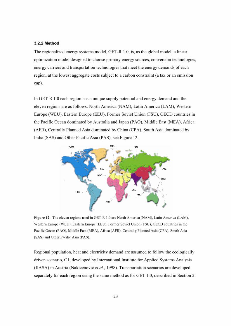
In GET-R 1.0 each region has a unique supply potential and energy demand and the
eleven regions are as follows: North America (NAM), Latin America (LAM), Western
Europe (WEU), Eastern Europe (EEU), Former Soviet Union (FSU), OECD countries in
the Pacific Ocean dominated by Australia and Japan (PAO), Middle East (MEA), Africa
(AFR), Centrally Planned Asia dominated by China (CPA), South Asia dominated by
India (SAS) and Other Pacific Asia (PAS), see Figure 12.
Figure 12. The eleven regions used in GET-R 1.0 are North America (NAM), Latin America (LAM),
Western Europe (WEU), Eastern Europe (EEU), Former Soviet Union (FSU), OECD countries in the
Pacific Ocean (PAO), Middle East (MEA), Africa (AFR), Centrally Planned Asia (CPA), South Asia
(SAS) and Other Pacific Asia (PAS).
Regional population, heat and electricity demand are assumed to follow the ecologically
driven scenario, C1, developed by International Institute for Applied Systems Analysis
(IIASA) in Austria (Nakicenovic et al., 1998). Transportation scenarios are developed
separately for each region using the same method as for GET 1.0, described in Section 2.

24
The same values have been used in all regions for investment costs, energy conversions
and fuel infrastructure. Regionalized load factors for solar energy technologies give some
advantages to the four regions Middle East and North Africa, Africa, Latin America and
North America.
It takes time to make profound changes in the energy system of the world. This inertia is
captured using maximum expansion constraints on how fast new technologies might
enter and we have assumed that 50 years is required for the development of a completely
new energy system. The maximum expansion rate can be set as a global or as a regional
constraint. If a global maximum expansion rate is chosen, the model will choose to
expand technologies in regions where it is most cost-efficient, i.e. solar energy will
expand at a faster rate in sunnier regions than what happens if regional expansion rate
constraints are chosen. In this study we use the global maximum expansion rate as our
base case, but we will also present some interesting differences to the base case using the
other method of a regionalized maximum expansion constraint.
3.2.3 Main results
In order to stabilize atmospheric CO2 concentrations at 400 ppm, approximately 500 GtC
(billion ton carbon) may be emitted over the period 1990-2100, (IPCC, 1994). The
following describes a global scenario (where the eleven regional results have been added
together) in which this CO2-reduction happens in a cost-effective manner.
The use of all renewables displays an increasing pattern throughout the century, where
biomass and solar energy plays the most important role. Over the next fifty years, a rapid
increase of biomass supply appears until the limitation of 200 EJ/year is met, thereafter
solar energy for hydrogen production increases during the second half of the century. The
use of oil and gas remains roughly constant until they become exhausted, by 2070-2090.
The use of coal remains possible since carbon capture and storage technologies are used
on a larger scale, from the middle of the century and onwards.

25
Oil and natural gas are phased out and biomass and coal dominate as primary energy
sources for heat production. For electricity production oil is phased out early and by the
end of the century coal with carbon capture and storage technologies become cost-
effective. By the end of the century the use of natural gas is declining due to lack of
availability. When solar based hydrogen is introduced by the middle of the century it will
rapidly increase its share. All renewable energy sources, display an increasing pattern
throughout the century. Wind and hydro power are used to their exogenously set
maximum level.
The fuel use in the transportation sector is aggregated in four sub sectors, cars, freight
aviation and rail. The rail sector is run on electricity and in the aviation sector there is a
transition from fuels based on oil towards liquefied hydrogen. In cars and freight sectors
a transition from petroleum-based fuels in internal combustion engines to hydrogen used
in fuel cell engines, in the middle of this century. Some methanol in internal combustion
engines will be used in the transition period in both sectors. The model also presents a
short period of natural gas as a cost-effective transition fuel, in the sector cars.
The major impact of different ways of setting the maximum expansion rates is where solar
hydrogen is being produced. Using a global maximum expansion rate, the region Middle
East and North Africa (MEA) will extract almost 200 EJ/yr of solar produced hydrogen, in
the year 2100, out of which 160 EJ/yr will be exported to other regions. Using a regionally
set maximum expansion rate MEA will only produce solar hydrogen for its own need. The
differences in primary extraction for MEA due to choice of expansion constraints, are
illustrated in Figure 13.

26
Figure 13. Primary energy extracted in region Middle East and North Africa, MEA. Solar produced
hydrogen will be exported in the case of a global maximum expansion rate.
The Asian regions Centrally Planned Asia dominated by China (CPA), South Asia
dominated by India (SAS) and Other Pacific Asia (PAS) are examples of regions which
import hydrogen in the case of a global maximum expansion constraint and produce their
own solar hydrogen in the other case, as illustrated in Figure 14.
Figure 14. Primary energy sources to supply the energy demand in the Asian regions. No solar produced
hydrogen will be developed in the case of a global maximum expansion rate. Instead hydrogen will be
imported mainly from MEA. In the case of a regional maximum expansion rate the Asian regions will
produce their own solar hydrogen.
One general result from this study is that it is possible to combine ambitious climatic
goals with an increased demand for energy services, but below, we will answer the four
questions asked in this study. The model results are explained in Section 4.

27
Question 1: When is it cost-effective to carry out the transition away from gasoline
and diesel?
In both GET 1.0 and GET-R 1.0 the general pattern is that oil remains the dominant fuel,
in the transportation sector, until 2030-2050, when a large scale transition to solar based
hydrogen is initiated. Oil based transportation fuels are fully replaced by 2080-2090.
Question 2: To which transportation fuel is it cost-effective to shift?
Solar based hydrogen becomes the dominant fuel in the transportation sector at the end of
this century.
Question 3: Will the cost-effective choice of fuel in the transportation sector be
different if a globally aggregated model is used rather than a regionalized version?
No, when adding the eleven regional results together to produce a global scenario, the
results of GET 1.0 and GET-R 1.0 are very similar.
Question 4: How will the method of regionalization affect transportation fuel
choices and trade in energy carriers?
Both methods of regionalization produce the same overall pattern of transportation fuel
choices, but the intercontinental trade in energy carriers will be different. The major
impact of different ways of setting the maximum expansion rates is where solar hydrogen
is being produced, as illustrated in Figure 13 and 14.
3.2.4 Future work
In a revised version of this study we have planned to regionalize the most recent GET
model version, GET 6.0, to investigate if the regionalized results remain.
In the current study, it is assumed that there is a carbon constraint applied to all regions of
the world. In the revised study, we intend to analyze fuel choices in the transportation
sector under the more realistic assumption that developing countries adopt abatement
policies perhaps a decade or two after the industrialized countries.

28
Further it could be of interest to look more into biomass supply and conversion options.
In this study biomass is a collective name for forest biomass, energy crops and biomass
residues. The end-use sector heat is a collective name for industrial process heat and
residential heating (including district heating). If the model were developed by more
supply and end-use options, it could maybe give another picture of the most cost-efficient
use for biomass.
3.3 Paper III: Biomass for heat or transport – an exploration into the
underlying cost dynamics in the GET model
3.3.1 Background and research question
In this study we want to achieve more detailed results on the cost dynamics in the GET
model in order to get a deeper understanding on why biofuels are not found to be a cost-
effective fuel choice.
3.3.2 Method
The analysis is carried out using a further developed version of the model, GET 5.1 and a
simplified model implemented in Excel. There are four main new features in the GET 5.1
model, compared to GET 1.0: (i) waste heat generated in the production of biofuels may
be sold to the heat market, (ii) carbon and capture storage technology can be applied on
both biomass and fossil fuel use, (iii) a split of the primary energy “oil” into two primary
oil sources, conventional and heavy oils and (iv) a further development of the refinery
process in the model. The main difference with these two latter new features is that it has
become more expensive to produce oil based transportation fuels. In earlier versions of
the GET model 100% of the primary energy “oil” could be converted into transportation
fuels, at a certain cost. Now, only 60% of the conventional oil can be converted into
transportation fuels, at that cost.

29
Parameter values are identical to those described in Azar et al. (2005) with two minor
changes. First the life times on truck engines have been shortened to 10 years instead of
15 years as in earlier GET models, following Kågeson (2004). Secondly we have
changed the energy efficiency on fuel cells in cars, compared to internal combustion
engines, from a factor of 2.2 more efficient down to a factor of 1.5, also following
Kågeson (2004). Hence, a transition into hydrogen in fuel cell vehicles is in the GET 5.1
model less favorable than in earlier versions of the GET model.
One important observation for the understanding of the underlying cost dynamics in the
GET model is that the primary energy price, P, [USD/GJ] in the GET 5.1 model, consists
of three parts, as
TSRC PPPP ++= ,
where PC is the primary energy cost including the extraction costs and distribution, PSR is
a scarcity rent11, generated in the model, and PT is a carbon tax on fossil fuel emissions.
The primary energy cost, PC, on conventional oil is taken from the GET 5.0 model (Azar
et al., 2005) and the primary energy cost on heavy oils is estimated following EIA (2002)
and in the model set to 3.5 USD/GJ 12 and 5 USD/GJ respectively. Primary energy cost
on biomass is set to 2 USD/GJ, natural gas is set to 2.5 USD/GJ and coal is set to 1
USD/GJ following Azar et al. (2005).
In the simplified model, implemented in Excel, we use parameter values and equations
equivalent to the GET 5.1 model and we calculate the cost per km for all fuel and vehicle
choices, see Table 1.
11 Scarcity rent (or scarcity value) is the economic term for the additional cost, added to the primary energy cost, due to the fact that the relative price on an item increases as a result of its relatively low supply, e.g. an exhaustible resource or raw materials in high demand. 12 In reality, the extraction cost is only a few dollars per barrel (corresponds to 0.1-0.4 USD/GJ) in the Middle East and higher in other major oil producing regions. The price observed in the market is much higher still and reflects scarcities and the fact that oil supply is controlled by a cartell (OPEC). It would be too complicated in a model like this to simulate the price setting behaviour of a cartell. For that reason, we have chosen to set the primary energy cost, PC , (extraction cost and distribution) for conventional oil at 3.5 USD/GJ. This oil price, which prevailed towards the end of the 90s, includes the impact of the cartell's activities. When oil reserves decline the scarcity rent will increase. We get roughly the same price development for oil (P=PC+PSR) in our model even if we put the extraction cost to zero.

30
Table 1. Derived total cost for each fuel choice used in either internal combustion engines or in fuel cell
engines. Costs are derived using primary energy costs PC , i.e., without scarcity rents and carbon taxes.
Year 2000 [USD/GJ] Total costb) [USD/km]
Fuel production
cost a) Internal com-
bustion engines Fuel cell engines Oil Conventional_gasoline 10.29 0.139 0.154 Oil Conventional_costly refinery_gasoline 12.24 0.146 0.159 Oil Heavy_gasoline 11.96 0.145 0.158 Oil Heavy _costly refinery gasoline 13.91 0.151 0.164 Natural gas 8.90 0.140 - Biomass_methanol 11.69 0.149 0.158 Natural gas_methanol 9.97 0.143 0.153 Coal_methanol 10.02 0.143 0.153 Biomass_hydrogen 15.92 0.171 0.161 Natural gas_hydrogen 12.76 0.160 0.154 Coal_hydrogen 13.53 0.163 0.155 Oil Conventional_hydrogen 14.89 0.168 0.158 Oil Heavy_hydrogen 17.37 0.176 0.164 Solar_hydrogen 31.04 0.223 0.196 a) includes the investment cost of the energy conversion plant, the operation and maintenance cost, the primary energy cost per energy output and the distribution cost to fuel stations. b) includes the fuel production cost, the vehicle investment cost, an engine efficiency factor, vehicle annual energy demand and engine life times
3.3.3 Main results
In the base case run of the GET 5.1 model, aiming for 450 ppm, no carbon capture and
storage technology is included. Results on cost-efficient fuel choices in the transportation
sector are presented in Figure 15.
Cost-efficient global transportation fuelsat base case, in GET 5.1, 450 ppm (EJ/yr)
0
50
100
150
200
250
300
2000 2010 2020 2030 2040 2050 2060 2070 2080 2090 2100
Fuel choices in subgroup Cars only (EJ/yr)
0
10
20
30
40
5060
70
80
90
100
2000 2010 2020 2030 2040 2050 2060 2070 2080 2090 2100
Figure 15. Cost-efficient transportation fuels, in the base case scenario, using the GET 5.1 model and a)
shows the fuel choices for the whole transportation sector where the three subgroups: Cars, Freight and
Aviation are aggregated and b) shows the fuel choices for subgroup Cars only. Acronyms used in the figure
are: OIL_C= conventional oil, OIL_H= gasoline, diesel and kerosene produced from unconventional heavy
oils, IC= internal combustion engines and FC= fuel cell engines.
GASOLINE DIESEL in IC from OIL_C
NATURAL GAS in IC
SOLAR HYDROGEN
in FC
Fuel choices in subgroup Cars only (EJ/yr)
b)
TRAIN ELECTRICITY
GASOLINE DIESEL KEROSENE from OIL_C NATURAL GAS
HYDROGEN
OIL_H
a)

31
The same overall results as in previous GET model studies appear, i.e. that
gasoline/diesel remain for some decades in the transportation sector until the carbon
constraint becomes increasingly stringent and that solar based hydrogen dominates by the
end of this century. Biofuels do not appear as a cost-effective fuel choice. One significant
exception from previous GET model results is, however, that natural gas has taken a
larger share of the transportation fuels, which is a result of that only 60% of the
conventional oil can be converted to gasoline and diesel at conventional refinery cost, in
the GET 5.1 model, compared to 100% in earlier GET versions.
To analyze the underlying cost dynamics in the GET model we use the calculated total
costs [USD/km] in the simplified model, presented in Table 1, but instead of using the
primary energy costs, PC, we run the full GET model, aiming for 450 ppm, to obtain
shadow prices (scarcity rents) from the primary energy supply equation. In the base case
run of the GET 5.1 model scarcity rents are generated on natural gas, conventional oil
and biomass13.
These new costs, based on primary energy prices, P, (minus PT) are then plotted as a
function of the carbon tax [USD/tC] to illustrate how the relation between the costs per
km changes with higher carbon taxes. The scarcity rents generated in the run for a
specific time step are kept constant14 in each plot. Plots for time steps 2030, 2050, 2070
and 2090 are presented in Figure 16. The vertical dotted line in each graph marks the
generated carbon tax for the specific time step.
13 Scarcity rents are generated on biomass due to the fact that the demand for biomass exceeds the supply potential at high carbon taxes. When the model is run without restrictions on CO2 emissions, no scarcity rent is added to the biomass primary energy cost. 14 If the GET model were run with higher carbon taxes, scarcity rents on biomass would increase as a consequence of an even stronger competition for biomass. Thus, it is not possible to foresee any other GET results from the plots outside the intersection with the dotted vertical carbon tax curve.

32
Cost per km (fuel+infrastructure+vehicle) as a function of carbon tax in the year 2030
0.140
0.142
0.144
0.146
0.148
0.150
0.152
0.154
0.156
0.158
0 25 50 75 100 125 150 175 200 225 250 275 300
USD/tC
USD
/km
Cost per km (fuel+infrastructure+vehicle) as a function of carbon tax in the year 2050
0.145
0.150
0.155
0.160
0.165
0.170
0 50 100 150 200 250 300 350 400 450 500 550 600
USD/tC
USD
/km
Cost per km (fuel+infrastructure+vehicle)
as a function of carbon tax in the year 2070
0.150
0.160
0.170
0.180
0.190
0.200
0 100 200 300 400 500 600 700 800 900 1000 1100 1200
USD/tC
USD
/km
Cost per km (fuel+infrastructure+vehicle) as a function of carbon tax in the year 2090
0.150
0.160
0.170
0.180
0.190
0.200
0.210
0 140 280 420 560 700 840 980 1120 1260 1400 1540 1680
USD/tC
USD
/km
Figure 16. Costs per km (subgroup Cars only) using primary energy costs generated in the base case set up,
of the GET 5.1 model. Note that the scarcity rents generated in each time step are kept constant in each plot.
Acronyms used in the figure are: OIL_C= conventional oil, OIL_H= heavy oils, NG= natural gas, MEOH=
methanol, H2= hydrogen, IC= internal combustion engines and FC= fuel cell engines.
In Figure 16 it is shown that in the year 2030 (a) and the year 2050 (b) cars run on fossil
fuel options, i.e. gasoline and diesel from conventional oil and natural gas, have the
lowest cost per km up to the carbon tax level of (a) 150 USD/tC and (b) 350 USD/tC
when cars run on biomass based methanol have the lowest cost per km.
In Figure 16c it is shown that in the year 2070 cars run on fossil fuel options, i.e. coal
based methanol, gasoline and diesel derived from heavy oils and natural gas, have the
lowest cost per km up to the carbon tax level of 950 USD/tC when cars run on biomass
COAL-MEOH_IC
NG_IC
OIL_C_IC
BIO-MEOH_ICOIL_H_IC
b)
COAL-MEOH_IC
NG_IC
OIL_C_IC
SOLAR-H2_FC
OIL_H_IC
BIO-H2_FC
c)
BIO-MEOH_IC
COAL-MEOH_IC
NG_IC
OIL_C_IC
SOLAR-H2_FC
OIL_H_IC
d)
SOLAR-H2_IC
a)
COAL-MEOH_IC
NG_IC
OIL_C_IC
BIO-MEOH_IC
NG-MEOH_IC

33
based methanol have the lowest cost per km. Note that two other carbon neutral
alternatives are close to biomass based methanol in the year 2070, i.e. solar based
hydrogen in fuel cell vehicles and biomass based hydrogen in fuel cell vehicles.
In Figure 16d it is shown that in the year 2090 cars run on fossil fuel options, i.e. coal
based methanol and gasoline and diesel derived from heavy oils, have the lowest cost per
km up to the carbon tax level of 930 USD/tC when cars run on solar based hydrogen in
fuel cell vehicles have the lowest cost per km. Note that the cost per km on biomass
based methanol now is higher than solar based hydrogen, which is due to a high scarcity
rent on biomass (the generated primary energy price, P, on biomass is 37 USD/GJ in the
year 2090).
The intervals where a certain fuel has the lowest cost per km are identified for each time
step, by analyzing the plots presented in Figure 16, and then the identified intervals are
presented in bars as shown in Figure 17, where also the carbon tax generated in the GET
5.1 base case is plotted as a line curve above the bars.
The fuel range that crosses the carbon tax line curve will first and foremost be chosen in
the scenario in a linear optimization model. However, since the model has expansion rate
constraints a technology might enter some time steps earlier to be able to expand into
large volumes. This is the case with solar based hydrogen, which enters the scenario in
2060-2070, see Figure 15b, but crosses the carbon tax line curve, in Figure 17, first in the
year 2080. The model also has constraints on the rate of which a fuel can be phased out
which, together with the fact that capital decays exponentially, explains why
conventional oil remains in the transportation sector for some decades in the scenario
even though natural gas crosses the carbon tax line curve earlier, in Figure 17. The reason
for the increasing use of gasoline and diesel derived from conventional oil in the years
2060 and 2070, in the scenario for subgroup Cars, is that investments are made in new
refinery capacity to supply the Freight and the Aviation sector. Using some of the
capacity to produce gasoline/diesel for cars will lower the total energy system cost, but
that can not be seen in Figure 17.

34
Cost-efficient fuel choices at different CO2-taxes
0
500
1000
1500
2000
2500
3000
3500
2000 2010 2020 2030 2040 2050 2060 2070 2080 2090 2100
Figure 17. Fuel choices in the transportation sector (subgroup Cars only) for different carbon tax intervals
in the base case scenario, aiming for 450 ppm. For each time step the lowest fuel cost per km for a certain
range of carbon taxes are identified and plotted in bars. The carbon tax generated in the run is plotted as a
line curve in front of the bars, with the tax values marked with x. Acronyms used in the figure are: OIL_C=
conventional oil, OIL_H= unconventional heavy oils, MEOH= methanol and SOLAR-H2= solar based
hydrogen.
By studying Figure 17 it would be tempting to interpret the carbon tax intervals as that
biofuels would become a cost-effective fuel choice if the carbon tax would be higher than
150 USD/tC in the year 2030, but this can not be taken for granted. A run where the
carbon tax is locked to 160 USD/tC for the years 2010-2030, does not introduce any
biofuels. Instead, the primary energy price, P, on biomass increases to 4.4 USD/GJ
compared to 2.3 USD/GJ in the base case, which increases the cost on biomass based
methanol to 0.161 USD/km compared to 0.151 USD/km in the base case.
Fuel choices for different CO2 taxes
BIO
-MEO
H
BIO
-MEO
H
BIO
-MEO
H
BIO
-MEO
H
BIO
-MEO
H
SOLA
R-H
2
BIO
-MEO
H
BIO
-MEO
H
OIL_H
OIL_H
SO
LAR
-H2
SOLA
R-H
2
SOLA
R-H
2 O
IL_H
USD/tC
CO2 TAX IN GET 5.1
OIL_H
NATURAL GAS
OIL_C
OIL_C COAL-MEOH

35
Increasing the carbon tax to 400 USD/tC will still not introduce any biofuels. In this run
the competition, between biomass based heat and biofuels, is even stronger and the
primary energy price, P, on biomass has increased to 10.7 USD/GJ leading to a cost of
biomass based methanol at 0.190 USD/km. In this run the carbon tax level when biofuels
become cost-efficient, has moved up to 990 USD/tC for year 2030.
This evasive carbon tax level when biofuels become cost-efficient, compared to fossil
based fuels, is an effect of the system effect in the model. The tax level moves upwards
with increasing carbon taxes, since this leads to an increasing biomass primary energy
price in the model.
The system effect can also be understood by comparing the costs for the two competing
CO2-neutral energy options (solar and biomass) in the three energy demand sectors. In
the transportation sector, by going from biomass based methanol in internal combustion
engines (0.149 USD/km) to solar based hydrogen in fuel cells (0.196 USD/km), we get
an increase of the cost per km by a factor of 1.3. In the electricity sector by going from
biomass based electricity (11.4 USD/GJ) to electricity derived from solar based hydrogen
(25.8 USD/GJ) we get an increase of the cost per Joule by a factor of 2.3. In the heat
sector by going from biomass based heat (3.82 USD/GJ) to heat derived from solar based
hydrogen (23.6 USD/GJ) we get an increase of the cost per Joule by as much as a factor
of 6.2. Hence, biofuels are not introduced in the transportation sector since biomass is
most cost-effectively used in the heat sector.
Since the system effect in the GET 5.1 model prioritizes the limited biomass to the heat
sector it indicates that a situation in which biofuels enter the transportation sector should
involve other types of changes to the model, for example, other cost assumptions,
features, and/or constraints. To analyze under what circumstances biofuels could become
a cost-effective strategy to reduce CO2 emissions, we have carried out a sensitivity
analysis in the GET 5.1 model. We find that biofuels enter the transportation scenario, if
we assume a lower conventional oil supply potential, a larger biomass supply potential,
that waste heat generated in the production of transportation fuels may be sold to the heat

36
market and that 25% of all biomass used for heat production need to be refined. When
these four assumptions are put together, a large amount of biofuels, accounting for 44%
of total transportation fuel production by the year 2050, is used, see Figure 18
Cost-efficient global transportation fuelsusing the GET 5.1 model, 450 ppm (EJ/yr)
0
50
100
150
200
250
300
2000 2010 2020 2030 2040 2050 2060 2070 2080 2090 2100
Figure 18. Cost-efficient fuel choices in the transportation sector in a sensitivity run. In this run biofuels
account for 44% of total transportation fuels in the year 2050. Acronyms used in the figure are OIL_C=
conventional oil, OIL_H= unconventional heavy oils, FOSS-MEOH= methanol derived from fossil fuels
and BIO-MEOH= biomass based methanol, i.e. biofuels.
4. Explaining the model results The general result, on cost-effective fuel choices in the transportation sector, seen in this
thesis is that oil based transportation fuels, i.e. gasoline, diesel for Freight and Cars and
kerosene for Aviation, dominate until solar based hydrogen enters the transportation
sector in 2040-2050. In some run natural gas plays an important role but biofuels do not
enter in either of the GET model base case set ups. This result is explained in detail in
paper III of this thesis but it can also be understood by the rough explanations made in
the following subsections.
4.1 How can oil remain dominant in the transportation sector for
several decades despite the introduction of stringent climate targets?
A perhaps somewhat surprising result from the GET-models is that oil remains dominant
in the transport sector several decades ahead, despite stringent climate targets. Here we
offer two separate explanations for that result.
NATURAL GAS
OIL_H
TRAIN ELECTRICITY
OIL_C HYDROGEN
OIL_H BIO-
MEOHFOSS-MEOH
NATURAL GAS

37
4.1.1 A physical explanation
A physical explanation for that is that all known oil and natural gas reserves combined,
contain about 200 billion ton carbon (GtC). Since we allow about 400 GtC (in the form of
CO2) to be emitted during this century, it is possible to release more carbon than what
exists in the total reserves of oil and natural gas, and still stabilize the atmospheric CO2
concentration at an ambitious level (CO2 emissions from the use of coal will then of
course need to be less than 200 GtC, which implies clear deviation from business as usual
scenarios).
When CO2-neutral primary energy sources, e.g. biomass and wind power, replaces fossil
fuels for the production of heat and electricity, large amounts of CO2 emissions are
abated in these two sectors. This leaves space for CO2 emissions that is large enough for
oil to remain as a primary energy source several decades ahead, despite stringent climate
targets. The advantages of using oil in the transportation sector are larger than using oil
for heat or electricity production which explains the result that oil remains as the
dominant fuel in the transportation sector several decades ahead. Gasoline and diesel
emits large amount of CO2 but it is in general easier, from a technical and economical
perspective to abate CO2 emissions from other sources.
4.1.2 Energy conversion efficiency
The energy conversion efficiency becomes very important when using limited primary
energy sources. Generally it can be stated that it is always easier (and therefore often
cheaper) to convert a liquid raw material into a liquid fuel compared to convert a solid
material into a liquid fuel. Gasoline and diesel can be produced at about 90% conversion
efficiency from oil, but liquid transportation fuels from solid raw material can only be
produced at conversion efficiencies between 25-60%. It is therefore very difficult for all
fuel alternatives to compete with gasoline and diesel when it comes to production costs,
as long as the primary energy cost for oil is moderate. Comparing the two limited energy
sources oil and biomass, both can be used with high energy conversion efficiency for heat
production but oil has higher energy conversion efficiency, compared to biomass, when

38
producing transportation fuels. This explains why oil based fuels have an advantage over
other transportation fuels.
4.2 Why are not biofuels seen as a cost-effective strategy to reduce
CO2 emissions?
Biomass is a relatively cheap energy source and can already today be used for electricity
generation, heat production and for the production of transportation fuels. The global
biomass supply potential is large (we assume that 200 EJ/yr biomass, corresponding to
about 500 Mha15 land, can be used for energy purposes in future), but it is however not
large enough to supply the whole energy sector, which implies that competition for
carbon neutral energy such as biomass is likely to arise. Biomass can be converted to heat
at an efficiency of about 80-90% while conversion efficiencies for bio-electricity and
biofuels lies between 25-60%. The conversion efficiency may increase if co-generation of
heat and/or power is implemented with biofuel production, but the market for surplus
heat is uncertain. Biomass can almost always replace more16 fossil fuels if it is used for
heat production, compared to when biomass is used for the production of biofuels. This is
an important issue since biomass is a globally limited resource.
Using biomass to produce biofuels would imply that the heat demand would have to be
satisfied from other CO2-neutral sources (hydrogen from solar or fossil fuels with carbon
capture and storage technology), which would increase the overall cost of meeting the
energy demand. Biofuels are hence not seen as a cost-effective strategy to reduce CO2
emissions since biomass is more cost-effectively used for heat production.
15 We assume that 100 EJ/yr comes from the actual yield of 200 GJ/ha from 500 Mha and that 100 EJ/yr comes from biomass residues. 16 The conversion efficiencies for heat production from fossil fuels and biomass are roughly the same, which implies that 1 GJ biomass roughly replaces 1 GJ fossil fuels when used for heat production. The conversion efficiencies for the production of transportation fuels differ, where gasoline and diesel can be produced roughly twice as efficient from oil compared to biofuels from biomass, which implies that 1 GJ biomass roughly replaces 0.5 GJ oil when used for the production of transportation fuels.

39
5. Discussion In this section we discuss factors not considered in the GET model and how reasonable
some assumptions are in the model.
5.1 Factors not considered in the GET model
The energy system description in the GET model is a simplification of reality in many
ways, e.g., the number of available technologies is limited, demand is price-inelastic,
decisions in the model are only based on cost considerations, and there is no uncertainty
about future costs, climate targets or energy demand levels etc. The global energy system,
in GET, is then optimized with perfect foresight and with a single goal function. Thus,
the model is not attended as a tool for making forecasts of the energy system
development.
An energy-economy model like this is, however, useful for constructing and comparing
scenarios. The model makes it possible to quantitatively explore the role and cost-
efficiency of various technologies given different carbon emission constraints, resource
availabilities, and parameter values for technologies. The model can be seen as an
experimental box where we can investigate relations between subunits which otherwise
are not obvious.
Some factors difficult to take into consideration in a global model are for example:
• Valuation of energy security
• Public acceptance of new technologies
• Convenience aspects
• Alternatives may not be identical17 for customers
• Real decision making more complicated than cost-minimization18
17 It is for example difficult to model willingness of buying electric cars, which is an energy-efficient technology but not really comparable to current standard cars. 18 In a linear optimization model, the total cost is minimized, and therefore a specific fuel will always be selected even if it differs in cost by only one percent. In reality human choices are not that black and white. If the range of prices is narrow, people may choose the higher cost alternative.

40
• Future agriculture and industry policies
• The impact of lobby groups
• Political instabilities e.g. war
Neither of these factors are considered in the GET model. Adding a price premium for
these factors could help but it will also add uncertainties.
Cost-effectiveness in dealing with climate change is not the only criterion for fuel choices
in the transportation sector and biofuels may be chosen for other reasons. As mentioned
before, if technical, economical and social barriers of using hydrogen in the
transportation sector prove to be too difficult to overcome, biofuels or CO2-neutral
electricity are two very important alternatives when we run out of conventional oil. Also
three more commonly heard reasons for choosing biofuels are presented in the following
sections.
5.1.1 Surplus of cropland
Many industrialized countries have a surplus of cropland and the production of traditional
agricultural crops as feedstock for ethanol production can be attractive to farmers, since
this does not involve any major change in present agricultural practices. Surplus cropland
can also be used for the production of cellulosic crops for heat and electricity production
purposes and, as technologies become available, production of so-called second
generation biofuels such as FT-diesel, methanol and lignocellulose-based ethanol. This
requires, however, that farmers take decision in switching to new crops of which they
have limited experience and in many cases less flexibility, e.g., a willow plantation is
typically lasting for 20-25 years. This leads to reduced willingness to establish long-term
willow plantations, especially among grain producers with a high equipment capacity for
grain cultivation (Börjesson and Berndes, 2006).

41
5.1.2 Energy security
Energy security is also a possible objective that could be considered more important than
cost-efficient CO2 abatement. Most countries wish to become less dependent on imported
oil. If energy security is regarded an important objective, biofuels have a larger potential
than hydrogen to be introduced in the transportation sector in a short-term scenario.
However, one should also recall that measures aimed at reducing fuel demand are also
possible and may be equally or even more cost-efficient in improving energy security.
5.1.3 Barriers for biomass in the heat sector
If biomass for some reasons has difficulties to supply a large share of the heat demand,
biomass instead will likely be used for biofuels or for electricity generation. One current
barrier for a large-scale introduction of biomass for industrial heat production has to do
with the inconvenience of using solid fuels. A rapid switch from solid fuels to natural gas
has occurred during the last decades in many world regions where gas is available
(Gielen, 2004). Gaseous and liquid fuels are more convenient to use compared to solid
fuels and the industrial sector is currently willing to pay more for gaseous and liquid fuels
compared to solid biomass (on a per GJ basis). However, with an increasing carbon tax
the price difference may in the future be large enough to make this argument invalid.
5.2 Is it reasonable to assume that CO2-neutral hydrogen will
overcome its barriers and be available in the transportation sector?
In this thesis, we have found that biomass is most cost-efficiently used in the heat sector,
assuming that CO2-neutral hydrogen will be available at sufficiently low costs. It is
currently very difficult to judge how reasonable this assumption about the future is.
Fuel cells have been around since the 19th century and have been used successfully for
decades for power generation in spacecraft, but not yet in mass produced road vehicles.

42
Car companies have produced about 70 prototype fuel cell cars19 and trucks as well as
dozens of buses (Service, 2004). Energy and car companies have also built hydrogen
fuelling stations worldwide, with many more on the drawing boards (Cho, 2004), but fuel
cell reliability, life time and production cost still need to be improved (Service, 2004, Ny
Teknik, 2004).
In addition to fuel cells a second large barrier is the onboard storage. At room
temperature and atmospheric pressure, hydrogen takes up roughly 3000 times as much
space as gasoline containing the same amount of energy. That means storing enough of it
in a fuel tank requires compressing it, or liquefying it, or using some other form of
advanced storage system. Many options are promising, but some still have severe
drawbacks, such as requiring high temperature or pressures, releasing the hydrogen too
slowly, or requiring complex and time-consuming materials recycling (Service, 2004).
Each of the problems faced by the hydrogen economy, e.g. a simple and cheap way to
produce CO2-neutral hydrogen in large scale, hydrogen storage, fuel cells, safety, and
infrastructure, would be challenging on its own. For a hydrogen economy to succeed, all
of these barriers must be solved. One loose end could block a broad-based changeover
(Service, 2004). Currently hydrogen as a large scale energy carrier faces huge barriers
and it is not obvious that it will be available in a future transportation sector, at
reasonable costs. It is, however, a general opinion among car manufacturer that hydrogen,
in either fuel cells or in internal combustion engines, is an attractive long-term solution.
Clearly, the long run future is still in the open.
6. Conclusions Conclusions, drawn in earlier GET model studies, that have been re-confirmed in this
thesis are that (i) it is possible to decrease carbon dioxide emissions at the same time as
the demand for energy services increases, (ii) in the near term improved energy efficiency
19 Photos and description of more than 200 hydrogen cars and more than 200 hydrogen filling stations are presented at www.h2cars.de (H2cars, 2005).

43
and increased use of biomass are two promising options, (iii) to reach ambitious CO2
stabilization levels, a radical change of the energy system is needed, (iv) the required
changes are not likely need to occur by themselves, i.e. a wise use of global and regional
policy instruments will be necessary and (v) low20 carbon taxes (below 75 USD/tC) do
not generate sufficiently strong incentives to introduce biofuels.
New conclusions, drawn within the scope of this thesis, leads to a further refined picture
of earlier conclusions, i.e. that the results differ between the short and the long term as
well as between low and high carbon taxes.
• Biomass is most cost-effectively used for heat productions at low CO2 taxes, up to
about 75 USD/tC, as shown in both the GET and the BEAP models.
• The sector in which biomass is most cost-effectively used at higher CO2 taxes
depends on assumed possible energy carriers and technologies. If hydrogen and/or
electricity derived from carbon free energy sources will not be available in the
transportation sector, biofuels become an important option if low or zero carbon
emissions are to be achieved.
• If hydrogen is assumed to make it as an energy carrier in the transportation sector,
then cost assumptions on hydrogen production, fuel cells, storage options and
infrastructure will determine in which sector biomass will be used. Clearly, these
costs are currently very uncertain, so the long run future for the cost-effective
transportation fuel choice is still in the open.
• Regionalizing the GET 1.0 model will not affect the overall pattern of
transportation fuel choices, i.e. that gasoline/diesel remain for some decades in the
transportation sector until the carbon constraint becomes increasingly stringent
and that solar based hydrogen dominates by the end of this century. Biofuels do
not appear as a cost-effective fuel choice.
• In paper III, we have developed a method, implemented in Excel, which explains
the GET model result and gives deeper insights about the system effect. By
studying the cost dynamics in the GET model, i.e. comparing the generated total 20 Biofuels will not be introduced at high carbon taxes either, in the GET model, but in this thesis we found that the results for higher carbon taxes depend on assumptions on future energy carriers and technologies. At very low or zero carbon taxes biofuels may be cost-efficient if the primary energy cost on oil are high.

44
costs per km for each fuel choice and identify the carbon tax intervals for each
time step where biofuels have the lowest cost per km, we find that the required
carbon tax level where biofuels become cost-efficient compared to fossil based
fuels, is evasive. The tax level moves upwards with increasing carbon taxes, since
this leads to an increasing biomass primary energy cost in the model.
• In a sensitivity analysis, carried out in Paper III, we find that the model is
sensitive for some type of changes. If we assume a lower conventional oil supply
potential, a larger biomass supply potential, that waste heat generated in the
production of transportation fuels may be sold to the heat market and that 25% of
all biomass used for heat production need to be refined, and combine these four
assumptions a large amount of biofuels will enter the transportation fuel scenario.
We have, however, not looked into how reasonable these new assumptions are
and neither analyzed possible barriers for introducing them.
7. Some implications for policy
7.1 Policy instruments for the transportation sector
Optimization models are useful and important tools for insights, but model results should
be treated with care. The model results highlight cost-effective pathways to low CO2
emission futures. This does not mean, however, that we suggest that governments should
adapt policies that make sure that these particular futures materialize, e.g. maintain the
dominance of oil based transportation fuels for several decades. Instead our view is that
policies should be implemented with the long-term goal of bringing down the CO2
emissions from the transportation sector to a low stabilization target and CO2 emissions
from the transportation sector can be reduced by (i) turning the vehicle fleet more energy-
efficient, (ii) changing transportation patterns, and (iii) changing from fossil based fuels
into CO2-neutral alternatives.

45
The fact that carbon taxes do not generate sufficiently strong incentives21 to introduce
biofuels in the model does not mean that biomass should not be used in the transportation
sector, since cost-effectiveness in dealing with climate change is not the only criterion for
policy makers. Rather, the implication is that if governments would want to see biofuels
take off, then they would probably also need to introduce complementary policies (e.g.,
mandatory blending). Whether this should be done or not is a prescriptive question which
lies outside the scope of this thesis.
7.2 Bring down costs for all promising CO2-neutral options
One misinterpretation of our result has been that no new technologies in the
transportation sector would need to be developed until the middle of the century. But
even though oil may remain as a dominant fuel for several decades it is important to
continue research, development and demonstration of alternative fuels and vehicles. A
fuel and technology transition in the transportation sector may take longer time than a
fuel transition in the two other sectors, since three separate parts of the transportation
system, i.e. fuel production, infrastructure and vehicles, need to be transformed almost
simultaneously. Since it still is an open question, whether CO2-neutral hydrogen will be
available in the transportation sector at sufficiently low costs, policies at present should
primarily aim at trying to bring down costs for all promising CO2-neutral options, e.g.
biofuels, electricity and hydrogen.
7.3 Policy instruments for the energy system
To realize ambitious climatic goals, a wise use of global and regional policy instruments
will be necessary to achieve a large transition of the whole energy system. These policy
instruments should cover three main areas (i) increase the cost for emitting fossil carbon
e.g. a CO2 tax, (ii) steer towards energy efficiency, e.g. introduce fuel consumption
standards and (iii) support research, development and diffusion of new advanced energy
technologies (Sandén & Azar, 2005). 21 Assuming that other CO2-neutral fuel alternatives are available. If no other alternatives are available high carbon taxes will generate sufficiently strong incentives to introduce biofuels.

46
Acknowledgement Ten years ago I was responsible for the Volvo Truck Corporation’s Art Service account
at Lennart Larsson advertising agency. I had signed a professional secrecy, to be able to
check the photographic quality of all new confidential cars, trucks and buses. I was
fascinated by all these new concept vehicles running on new engines and alternative fuels.
At that time I would never have guessed that I ten years later would be doing research on
energy systems and that I would be invited to the Swedish Parliament to talk about
alternative transportation fuels. Thank you Carina Möller-Liderfors, Lisa Andersson and
Anna Järvholm for your ongoing friendship including our fifteen year tradition of
Christmas candy production. I’m very grateful for your support when I decided to totally
change careers, at that time with the goal of becoming a math and science teacher.
Sending in my resignation, ten years ago, was the first, and maybe the most difficult, step
to carry out towards writing this thesis.
I would like to offer a special thanks to Roy Tärneberg, my teacher in Physics during the
preparatory year in Science. You have a remarkable enthusiasm and you inspired me to
look for a university program that included more Physics than the teacher education
offered.
I also would like to express my gratitude to Lena Gustafsson, professor of Biotechnology
and presently Vice President at Chalmers. You held an inspiring public lecture at
Vetenskapsfestivalen 1997, on how mutants of Saccharomyces cerevisiae (baker’s yeast)
could improve ethanol production from cellulose, and you mentioned that ethanol based
on cellulosic biomass could be an important substitute for gasoline in future. Thanks to
that lecture I knew what I would like to work with after finishing a university program.
Being involved in energy research preferably with a connection to transportation fuels
became my highest goal.
I studied an interdisciplinary university program called “Problem Solving in Science”, at
Göteborg University, and during my first year I came in contact with the department of
Physical Resource Theory. Thank you Björn Sandén for being a fantastic supervisor for

47
me and my student group and Christian Azar for not just being an inspiring teacher but
also for asking me to work for you during my student time, which was very interesting
and highly instructive. Also thanks to all other brilliant teachers I met during the
university program, especially Maria Sundin, Ann-Marie Pendrill and Maj Hansson, your
knowledge and enthusiasm have made a deep impression on me. Further thanks to all my
classmates and friends; Björn Adolfsson, Igor Anakijoski, Daniel Andersson, Peo Björck,
Samuel Brohede, Filip Edström, Mikael Ekenstam, Erik Filipsson, Julia Franzén, Fredrik
Hedenus, Stina Hemdal, Jakob Heydorn Lagerlöf, Stefan Högberg, Charlott Johansson,
Hanna Jönsson, Marcus Krantz, Milcco Larsson, Lena Lundqvist, Elin Löwendahl, Björn
Persson, Martin Persson, Lotta Svensson, Camilla Thulin, Luis Young, Frida Wahl and
Johan Österman for the terrific mix of serious studying and fun parties. Björn, Erik and
Peo, I will always remember our study trip to the Ruhr-area in Germany where we took a
close look at hydrogen pipelines. Great fun.
To enter deeper into optimizing theory I took a Postgraduate Diploma in Statistics and
Operation Research by studying one year at Royal Melbourne Institute of Technology in
Australia. A special thanks to Denise and David who became, and still are, dearest
friends to me and my family. Denise, I love you! Are you coming over for some
champagne tonight? Thanks also to Astrid Linder who is another very good Australian
(and Swedish) friend always very interested in my PhD-studies. Astrid, I admire your
energy, your hard work and your fabulous results. Torbjörn and Susanne Bladby, our
friendship was also initialized during the year in Australia and means a lot to me.
Susanne, are you ready for a game of Rummy?
Soon after returning to Sweden, I started my position as a PhD-student at the department
of Physical Resource Theory. I would like to thank everyone I have come to know, both
currently and previously working at the department, for making it such a stimulating
environment as it is. Thank you Karl-Erik Eriksson, Eija Hyttinen, Jenny Hanell,
Bernhard Mehlig, Johan Stäring, Peter Nordin, Krister Wolff, Peter Jönsson, Jessica
Johansson, Fredrik Fredriksson, Tomas Kåberger, Björn Sandén, Ingrid Råde, Johan
Swahn, Pia Sundh and Elin Löwendahl for your contribution to the FRT-atmosphere. I

48
wish you all luck in the future at your new positions. Also thanks to Professor Dean
Abrahamson and Professor Bob Ayres for your regular visits to the department and for
sharing your great knowledge with us. Thank you Sten Karlsson, for your never-ending
interest in all subjects and every seminar. Your sharp comments and questions always
enrichen our discussions, which lead to improved research. Also thanks to John
Holmberg, for being an excellent head of the department, which demands a large amount
of time and patience. Your development of the department, as well as us individuals, is
gratefully acknowledged. A special thanks to Tobias Persson and Julia Hansson for being
the best conceivable room mates. You are always in a good mood and loaded with good
arguments on every discussion subject. I really enjoy working close to you. Thank you
Sandra Malentacchi, Fredrik Hedenus, Frances Sprei, Martin Persson, Daniel Johansson,
Jonas Nässén, Wathanyu Amatayakul, Stefan Wirsenius, Ulrika Lundqvist, Martin Jacobi,
Anders Eriksson, Claes Andersson, Olof Görnerup, Kolbjørn Tunstrøm and Johan
Nyström for your support, friendship and laughter. You all contribute to an inspiring
environment and I hope to spend some more years with you at the department.
I would like to offer special thanks to my supervisors and co-authors. Dolf Gielen, your
quick responses to my many questions as well as your clear-sighted and thorough
comments are gratefully acknowledged. Per Kågeson, your knowledge about vehicles and
transportation systems has had a deep impact on me. Göran Berndes, your guidance is a
splendid mix of rapid funny replies and thoughtful words of wisdom. Kristian Lindgren, I
am particularly grateful for your excellent, calm and encouraging guidance. Thank you
for letting me share your office for six months. Last but not least thank you Christian
Azar, my main supervisor, for all inspiration and support. You have a fantastic gift to
explain things in a simple and pedagogical way. Your intellect, humour, ambition and
knowledge have made a deep impression on me. You inspire me.
Financial support from Swedish Agency for Innovation Systems, Vinnova, and Swedish
Energy Agency is gratefully acknowledged. Without your funding this thesis would not
have been materialized.

49
I would also like to thank my family whose support means a lot to me; Ulla Lidbeck,
Sven Holländer, Thomas Lidbeck, Anette Aretjäll, Camilla and Thomas Bako, Lena and
Daniel Roos. Thanks also to the whole “Grahn-clan” especially my parents in-law Rosa
and Gerhard Grahn.
Emma and Viktor, by your appearance you have richened my life. I love you and wish
you the very best of futures.
Finally and most importantly, thank you Roberto for being the most generous,
considerate, handy, well-informed and sharp man I have ever met. I love you!

50
References
Azar C, K Lindgren and B A Andersson (2000). “Hydrogen or methanol in the
transportation sector?”, Department of Physical Resource Theory, Chalmers
University of Technology, Göteborg, Sweden.
Azar C, K Lindgren and B A Andersson (2003). “Global energy scenarios meeting
stringent CO2 constraints - cost-effective fuel choices in the transportation sector”,
Energy Policy 31(10), 961–976.
Azar C, K Lindgren, E Larson and K Möllersten (2005). “Carbon capture and storage
from fossil fuels and biomass - costs and potential role in stabilizing the
atmosphere”, Climatic Change, (in press).
Azar C and H Rodhe (1997). “Targets for Stabilization of Atmospheric CO2” Science
276(5320), 1818-1819.
Berndes G, M Hoogwijk and R van den Broek (2003). ”The contribution of biomass in
the future global energy supply: a review of 17 studies” Biomass & Bioenergy
25(1): 1-28.
BP (2001). “British Petroleum statistical review of world energy 2001”, printed in
England by Beacon Press. Available at www.bp.com.
BP (2005). “British Petroleum statistical review of world energy 2005”, printed in
England by Beacon Press. Available at www.bp.com/statisticalreview.
Börjesson P and G Berndes (2006). “The prospects of willow plantations for wastewater
treatment in Sweden”. To appear in Biomass & Bioenergy.
Cho A (2004). “Fire and ICE: Revving up for H2”, Science vol 305, p 964-965.

51
EIA (2002). “International Energy Outlook, 2002”, Energy Information Administration –
Official Energy statistiscs from the U.S. Government, World resources,
Washington, USA, Available at www.eia.doe.gov.
European Council (2003). “Directive 2003/30/EC of the European parliament and of the
council of 8 may 2003 on the promotion of the use of biofuels or other renewable
fuels for transport”, Official Journal of the European Union, L 123/42, 17.5.2003.
Available at
http://europa.eu.int/comm/energy/res/legislation/doc/biofuels/en_final.pdf.
European Council (2005). “Presidency conclusions to delegations, 7619/1/05 REV 1,
Brussels 22 and 23 March 2005”. Available at
http://ue.eu.int/ueDocs/cms_Data/docs/pressData/en/ec/84335.pdf.
FAOSTAT (2001a). “Agricultural and forestry statistics 2001”. United Nations Food and
Agricultural Organization, Rome. Available at www.fao.org.
FAOSTAT (2001b). “Food balance sheets 2001”. United Nations Food and Agricultural
Organization, Rome. Available at www.fao.org.
Gielen D J, J Fujino, S Hashimoto and Y Moriguchi (2002). “Biomass strategies for
climate policies?”, Climate Policy 2(4), p.319-333.
Gielen D J, J Fujino, S Hashimoto and Y Moriguchi (2003). “Modeling of global biomass
policies”, Biomass & Bioenergy 25(2), p.177-195.
Gielen D J (2004). IEA, International Energy Agency, Paris, France. Email
correspondence, 8 Aug 2004.

52
Goldemberg J, S T Coelho, P M Nastari and O Lucon (2004). “Ethanol learning curve –
the Brazilian experience” Biomass and Bioenergy 26, p.301 – 304.
H2cars (2005). “Overview of hydrogen cars and hydrogen filling stations”. A service by
L-B Systemtechnik and HyWeb, Germany. Retrieved Aug 2005, from
www.h2cars.de.
Hamelinck C (2004). “Outlook for advanced biofuels”, PhD thesis, Utrecht University,
The Netherlands, ISBN: 90-393-3691-1.
Harvey D (2000). “Global warming – the hard science”, Pearson Education, Prentice Hall,
Singapore, ISBN: 0582-38167-3.
IPCC (2001a). “Synthesis Report of the Intergovernmental Panel on Climate Change”,
Cambridge University press, New York. Graphics retrieved July 2005 from
www.ipcc.ch.
IPCC (2001b). “Climate Change 2001 - the scientific basis”. Contribution of working
group I to the Third Assessment Report of the Intergovernmental Panel on Climate
Change, Cambridge University press, New York.
IPCC (1994). “Climate Change 1994 – Mitigation”. Contribution of working group III to
the third assessment report of the Intergovernmental Panel on Climate Change,
Cambridge University Press, UK
Kågeson Per (2004). Nature Associates, Stockholm, Sweden. Personal communication,
19 Jan 2004.

53
Marland G, T A Boden and R J Andres (2002). “Global, Regional and National Fossil
Fuel CO2 emissions”. In Trends: A Compendium of Data on Global Change.
Carbon Dioxide Information Analysis Center, Oak Ridge National Laboratory, U.S.
Department of Energy, Oak Ridge, Tennessee, U.S.A. Available at
http://cdiac.esd.ornl.gov/trends/trends.htm.
Nakicenovic N, A Grubler and A McDonald (1998). “Global Energy Perspectives”.
Cambridge University Press. Scenarios from the report are also presented at
www.iiasa.ac.at/collections/IIASA_Research/Research/ECS/docs/book_st/node2.ht
ml.
NE (2005). Nationalencyklopedin. Electronic version based on twenty printed volumes of
the Swedish National Encyclopedia. Information retrieved Nov. 2005, from
www.ne.se.
Ny Teknik (2004). “Europa halkar efter i bränslecellsracet” Article in Swedish written by
Norbert Andersson. Published 27 May 2004. Also available at
www.nyteknik.se/pub/ipsart.asp?art_id=34949.
O’Neill B C and M Oppenheimer (2002). “Dangerous Climate Impacts and the Kyoto
Protocol”, Science vol 296, p. 1971-72.
Sandén B.A. and C. Azar (2005). “Near-term technology policies for long-term climate
targets – economy wide versus technology specific approaches”, Energy Policy
33(12): 1557-1576.
Service R F (2004). “The Hydrogen Backlash”, Science vol 305, p 958-961.
UN (1999). “Industrial commodity statistics yearbook 1997”. United Nations, New York.

54

Paper I


Paper I. Grahn et al, “Biomass for heat or as transportation fuel? – a comparison between two model based studies”, Submitted to Biomass and Bioenergy 2005
1
Biomass for heat or as transportation fuel? – a comparison between two model based studies
Maria Grahna), Christian Azara), Kristian Lindgrena), Göran Berndesa), Dolf Gielenb),
a) Department of Energy and Environment, Physical Resource Theory, Chalmers University of Technology,
412 96 Goteborg, Sweden, E-mail: [email protected]
b) International Energy Agency, 75739 Paris Cedex 15, France, E-mail: [email protected]
Abstract In two different energy economy models of the global energy system, the cost-effective use of
biomass under a stringent carbon constraint has been analyzed. Gielen et al conclude that it is
cost-effective to use biofuels for transportation, whereas Azar et al find that it is more
cost-effective to use most of the biomass to generate heat and process heat, despite the fact that
assumptions about the cost of biofuels production is rather similar in the models. In this study,
we compare the two models with the purpose to find an explanation for these different results. It
is found that both models suggest that biomass is most cost-effectively used for heat production
for low carbon taxes (below 50-100 USD/tC, depending on the year in question). But for higher
carbon taxes the cost effective choice reverses in the BEAP model, but not in the GET model.
The reason for that is that GET includes hydrogen from carbon free energy sources as a
technology option, whereas that option is not allowed in the BEAP model. In all other sectors,
both models include carbon free options above biomass. Thus with higher carbon taxes,
biomass will eventually become the cost-effective choice in the transportation sector in BEAP,
regardless of its technology cost parameters.
Keywords: Energy scenarios, Energy system model, Biomass, Alternative transportation fuels,
Liquid biofuels, Hydrogen, Carbon dioxide emissions, Carbon tax

Paper I. Grahn et al, “Biomass for heat or as transportation fuel? – a comparison between two model based studies”, Submitted to Biomass and Bioenergy 2005
2
1. Introduction Due to the expected increase in global energy demand, the supply of CO2-neutral energy may
have to grow to levels similar to or even larger than the present global total fossil fuel use, if we
are to avoid venturing into a future with a doubled, tripled or even quadrupled pre-industrial
atmospheric CO2 level. Among several candidates capable of supplying large amounts of
CO2-neutral energy, biomass ranks as one of the few options already competitive on some
markets. It is a low cost renewable fuel, and it is near penetration into new applications as
policies, markets and related technologies develop.
There are large uncertainties about the potential for biomass, but it is nevertheless clear
that the potential supply is low compared to the future required levels of climate neutral energy,
almost regardless of whether one is optimistic or pessimistic about the global bioenergy
potential (see, e.g., Azar 2005, Berndes et al, 2003). Biomass will thus not be available for all
possible energy applications and it is therefore important to discuss where to use the scarce
biomass resources for climate change mitigation.
In their study of cost-effective fuel choices in the transportation sector, Azar et al (2003)
find that it is more cost-effective to substitute biomass for fossil fuels in power and heat
production (Azar et al, 2003). Oil based fuels remain in the transportation sector for the next
four to five decades and thereafter solar hydrogen or hydrogen produced from fossil fuels with
carbon capture and storage enters. However, in another study, Gielen et al (2002, 2003)
conclude that, most of the biomass is cost-effectively used as biofuels1 for transport. These two
studies base their results on global energy system models developed especially for these studies.
Gielen et al have developed the BEAP (Biomass Environmental Assessment Program) model
and Azar et al the GET 1.0 (Global Energy Transition) model. The two models are in many
ways similar to each other and both models are run under ambitious constraints on carbon
dioxide emissions.
The aim of this paper is to compare the two models with the purpose to find an explanation
for the differing results.
The paper is structured as follows: In Section 2, we summarize the results by Azar et al and
Gielen et al. In Section 3 we briefly describe the two models and present main input data
1 In this paper “biofuels” always means liquid biofuels in the transportation sector.

Paper I. Grahn et al, “Biomass for heat or as transportation fuel? – a comparison between two model based studies”, Submitted to Biomass and Bioenergy 2005
3
assumptions and in Section 4 we identify four key reasons for the differing results. The impact
of using assumptions similar to the GET model is tested in the BEAP model. In Section 5 we
analyze how the GET model changes when using assumptions similar to the BEAP model and
in Section 6 we present an explanation for the differing results. Finally in Section 7 we discuss
the results and offer some conclusions for modelers and policy makers.
2. A summary of the two different model results In this section, we summarize results from the two models2. When presenting the results from
the GET model, we have used an updated version of the GET 1.0 model, thus the graphs shown
are very similar, but not identical to the results presented in Azar et al (2003). Details of GET
5.0 can be found in Azar et al (2005). The graphs for the BEAP model have been generated by
running version BEAP2100 with GLOB-policy (the runs were carried out by Maria Grahn). In
Figures 1a,b the global primary energy supplies are shown. Figures 2a,b show the
transportation sectors and Figures 3a,b show the biomass use in the two models. Both models
are run under stringent CO2 constraints. In the BEAP model a global carbon tax of
approximately 300 USD per ton C is applied from the year 2020 and onwards. The cumulative
emissions during this century amount to approximately 450 Gt C. This emission level
corresponds roughly to an atmospheric carbon dioxide concentration target of 400 ppm by the
year 2100. In the runs with the GET 5.0 model performed for the purpose of this paper, CO2
emissions were constrained by assuming a stabilization target by the year 2100 at 400 ppm.
Such a target might be required if we are to be relatively certain that we meet the EU target that
the global temperature increase should remain below 2oC (see Azar & Rodhe, 1997).
2 Results from the BEAP model and from the GET model have been published in Gielen et al (2002, 2003) and in Azar et al (2003).

Paper I. Grahn et al, “Biomass for heat or as transportation fuel? – a comparison between two model based studies”, Submitted to Biomass and Bioenergy 2005
4
BEAP Primary Energy Supply
0100
200300
400500
600700
2000 2010 2020 2030 2040 2050 2060
GET Primary Enery Supply
0
100200
300400
500600
700
2000 2010 2020 2030 2040 2050 2060 Fig. 1. Results on global primary energy supply as presented in a) the BEAP paper and in b) the GET paper. In both
models there is an increasing use of biomass to meet the stringent CO2 constraints. These are referred to as the
reference scenarios of the models.
BEAP Transportation fuel
020406080
100120140160
2000 2010 2020 2030 2040 2050 2060
GET Transportation Fuel
020406080
100120140160
2000 2010 2020 2030 2040 2050 2060 Fig. 2. Transportation fuels as presented in a) the BEAP paper and in b) the GET paper. In the BEAP model there
is an increasing use of biofuels , i.e. ethanol, methanol from biomass and diesel/gasoline from biomass via
HTU-oil (Hydro Thermal Upgrading). In the GET model there in not any biofuels in the base case run. These are
referred to as the reference scenarios of the models.
BEAP Biomass use
0
50
100
150
200
250
2000 2010 2020 2030 2040 2050 2060
GET Biomass use
0
50
100
150
200
250
2000 2010 2020 2030 2040 2050 2060 Fig. 3. Biomass use as presented in a) the BEAP paper and in b) the GET paper. In the BEAP model the largest
share of biomass is used for the production of fuels for transport but in the GET model the largest share of the
biomass is used for HEAT+ production (stationary energy use that neither aims at generating electricity nor
transportation fuels but mainly heat production). These are referred to as the reference scenarios of the models.
NUCLEAR COAL
BIOMASS HYDRO
SOLAR
NAT GAS OIL
a)
EJ/yr
OIL
COAL
NUCLEAR b)
NAT GAS
WIND
HYDRO BIOMASS
EJ/yr
GASOLINE/DIESEL
MEOH_NG MEOH_BIO
ETHANOL
a)
GASOLINE/DIESEL VIA HTU
EJ/yr
RAIL b)
GASOLINE/DIESEL/KEROSENE
H2
NG
EJ/yr
TRSP FUEL
HEAT+
NON-ENERGY USE
a)
EJ/yr
HEAT+
b)
EJ/yr
ELECTRICITY

Paper I. Grahn et al, “Biomass for heat or as transportation fuel? – a comparison between two model based studies”, Submitted to Biomass and Bioenergy 2005
5
In both models there is a steady increase in total biomass use, but fuel choices in the
transportation sector and what the biomass is used for differ between the two models (see
Figures 2-3). The result in the GET model, that hydrogen in the long run takes over as the fuel
for the transportation sector, remains unchanged under a variety of parameter choices. However,
during a transient phase other fuels, e.g. methanol or natural gas, play a significant role in some
runs.
3. Model descriptions Both models are global energy systems optimization models. The BEAP model is a mixed
integer programming (MIP) model and simulates an ideal market based on an algorithm that
maximizes the sum of the consumers’ and producers’ surplus. The GET model is a linear
programming model that is set up to meet exogenously given energy demand levels at the
lowest energy system cost. Both models exhibit so-called ‘perfect foresight’ which means that
all features of the model (future costs of technologies, future emission constraints, availability
of fuels etc) about the future isare known at all times.
The GET model includes constraints on the expansion rates for different primary energy
sources and energy technologies. In the GET model, there is only one aggregate heat and
process heat sector that includes all stationary use of energy that neither aims at generating
electricity nor at producing transportation fuels. We refer to this as HEAT+. The BEAP model
has a more careful treatment of the heat sector in that it distinguishes between industrial heat,
urban heat and rural heat. In order to facilitate comparisons between the models, we aggregate
energy demand into three main sectors: Electricity, Transportation fuels and HEAT+. The
primary energy supply options, the three energy demand sectors and fuel choices in the
transportation sector are roughly outlined in Figure 4.

Paper I. Grahn et al, “Biomass for heat or as transportation fuel? – a comparison between two model based studies”, Submitted to Biomass and Bioenergy 2005
6
Fig. 4. The basic flow chart of supply and fuel choices in both energy system models.
The BEAP model database, including the model output files, is available on the Internet (EMP,
2001). Details of the BEAP and GET models are available in Gielen et al, (2002, 2003) and
Azar et al (2000, 2003, 2005), respectively.
3.1. Assumptions on supply potentials
Resources on coal, oil, natural gas and biomass are considered limited and the supply potentials
assumed in both models are presented in Table 1, as well as the assumed primary energy cost.
Table 1. Supply potentials of limited resources and assumed primary energy cost
Supply potential
[EJ] Primary energy cost
[USD/GJ] BEAP GET BEAPc) GET Coal 22000 300000 1.8 2 Coal (additional) 230000 - 4.4 - Oil conventional 12000 12000 1.6 3 Oil other 14000 - 3.6 – 5.2 - Natural gas conventional 12000 10000 2.2 2.5 Natural gas other 11000 - 3.0 – 3.8 - Fuel wood [EJ/yr] 70a) - - -
Energy plantations & straw [EJ/yr] Not well definedb) -
-
-
Total biomass supply potential [EJ/yr] Not well defined b) 200
2.4
3
a) This refers to potential wood extraction in existing forests. b) The potential depends on land and biomass prices calculated by the model. c) In the BEAP model the primary energy cost depends on distance of transport. Mean values are presented.
Oil Coal
Natural gas Nuclear
Biomass Solar
Hydro Wind
Electricity HEAT+ (Heat and Other Fuel use) Transportation fuels
BEAP GET Gasoline/diesel X X Gasoline/diesel via HTU-oil (biomass based)
X
-
Methanol X X Ethanol X - Fischer-Tropsch diesel X - Hydrogen (fossil fuel based) X X Hydrogen (CO2-neutral) - X Natural gas - X
Energy Conversions

Paper I. Grahn et al, “Biomass for heat or as transportation fuel? – a comparison between two model based studies”, Submitted to Biomass and Bioenergy 2005
7
3.2. Assumptions on conversion efficiencies, investment costs and
production costs
The conversion efficiencies and investment costs of energy conversion plants are key factors
that determine the total production cost. Assumptions on O&M costs and plant life times can be
found in Gielen et al, (2002, 2003) and Azar et al (2005). Total production costs include
primary energy costs but exclude taxes, see Table 2.
Table 2. Investment costs, conversion efficiencies and production costs in the two models.
Conversion efficiency Capital cost Total production costa)
BEAP GET BEAP GET BEAP GET
η η [USD/kW]b) [USD/kW] USD/GJ USD/GJ
Coal Industrial heat 0.71 0.90 67c) 300 4.2 c) 3.2 Oil Industrial heat 0.83 0.90 34 c) 100 2.8 c) 3.7 Natural gas Industrial heat 0.91 0.90 17 c) 100 2.7 c) 3.1 Wood Industrial heat 0.71 0.90 84 c) 300 4.4 c) 4.3 Coal Urban heat 0.56 0.90 34 300 4.0 3.2 Oil Urban heat 0.80 0.90 0 100 3.2 3.7 Natural gas Urban heat 0.80 0.90 34 100 2.9 3.1 Wood Urban heat 0.67 0.90 34 300 4.9 5.4 Coal Electricity (conventional) 0.36 - 1009 - 8.4 - Coal Electricity (advanced) 0.45 0.45 1093 1100 7.7 7.6 Coal Electricity (with CO2 removal) 0.36 0.38 1682 1500 9.9 10.1 Oil Electricity 0.43 0.50 841 600 7.2 7.9 Natural gas Electricity 0.56 0.55 673 500 6.4 5.8 Natural gas Electricity (with CO2 removal) 0.48 0.47 1009 900 6.7 8.2 Wood Electricity 0.45 0.40 1346 1200 10.1 9.9 Coal Methanol - 0.60 - 1000 - 5.7E) Natural gas Methanol 0.67 0.70 673 600 4.8 5.3E) Sugar/starch Ethanol 0.56 - 841 - 6.0 - Wood Ethanol 0.33 - 1177 - 9.3 - Wood Methanol 0.56 0.60 1009 1000 7.2 7.8e) Wood Fischer-Tropsch diesel 0.50 - 1346 - 9.3 - Wood Gasoline/diesel via HTU-oil 0.56 - 841d) - 7.2 - Oil Gasoline/diesel n.a. 0.90 n.a. 1000 n.a. 6.2 Coal Hydrogen - 0.65 - 700 - 5.7e) Oil Hydrogen - 0.75 - 400 - 5.5e) Natural gas Hydrogen 0.78 0.80 336 300 4.2 4.3e) Wood Hydrogen - 0.60 - 800 - 8.0e) Solar Hydrogen - 1.00 - 2000 - 18.1e)
a) Total production costs depend on conversion efficiencies, investment costs, O&M costs, plant life times and primary energy costs, which vary between technologies. No taxes are included. b) Investment costs are in the BEAP model given in Yen per GJ. To be comparable, values have been converted in the following way: The cost in USD/kW is equal to the cost in Y/GJ multiplied by 0.008USD/Y and 31.54 GJ/kW and 1/LF where LF (load factor) assumed to 0.75 for all plants. c) Investment cost after the error has been corrected. d) The capital costs only consider the two plants for the production of a biocrude (505 USD/kW) and for upgrading the biocrude into a naphta-like product (336 USD/kW). Thereafter it is assumed that diesel and gasoline can be produced using existing steam cracking technology (Naber et al, 1999). e) To be able to compare the methanol and hydrogen costs per vehicle, one also has to consider costs for infrastructure, extra costs per vehicle, storage, fuel cells and efficiency change.

Paper I. Grahn et al, “Biomass for heat or as transportation fuel? – a comparison between two model based studies”, Submitted to Biomass and Bioenergy 2005
8
This table offers a first order explanation for the result in the GET model. In the near term, at a
zero CO2 tax, the cost of biomass based energy carriers is higher than all alternatives in all
sectors, but the difference between alternatives is smaller in the heat than in the transportation
sector. For that reason, biomass can replace fossil fuels in the heat sector at a lower cost
compared to replace fossil fuels in other sectors.
As the carbon constraint becomes increasingly stringent, or at higher CO2 tax, fuel changes
become necessary also in the transportation sector. Then hydrogen based on solar energy enters
the energy system. If biomass is used for transportation fuels, then hydrogen from solar energy
becomes necessary to satisfy the demand for HEAT+. This is, using our technology cost
parameters, more costly than using biomass for the HEAT+ sector and using the hydrogen in
the transportation sector. For that reason, hydrogen from solar becomes the cost-effective
choice in the long run in the GET model transportation sector.
3.3. Energy demand
In the GET model, electricity and HEAT+ demand levels are exogenous and taken from the
ecologically driven scenario C1 in IIASA/WEC (see Nakicenovic et al, 1998). The
transportation scenario is developed separately, assuming that increase in the amount of
person-kilometers traveled is proportional to the GDP growth (in PPP terms). Details of the
demand scenarios are available in Azar et al (2000).
The BEAP model covers the global energy, food and materials system. The demand for
food and materials are based on statistics from the Food and Agricultural Organization (FAO
2001a, 2001b) and United Nations (UN, 1999). The energy demand is based on the BP review
of world energy use (British Petroleum, 2001). Future demand in the base case is an
extrapolation of historical trends and forecast as a function of regional GDP growth and income
elasticities. Details on demand projections in the BEAP model are available in Gielen et al.,
(2003) and on the Internet (EMP, 2001).
In the BEAP study, price elasticities in the range of −0.1 to −1 have been used for all
demand categories. In the GET model energy efficiencies are assumed in the C1 demand
scenario and it is also assumed that there is an exogenous improvement in energy efficiency in
the transportation sector by 0.7% per year.

Paper I. Grahn et al, “Biomass for heat or as transportation fuel? – a comparison between two model based studies”, Submitted to Biomass and Bioenergy 2005
9
3.4. Constraints
Constraints have been added to both models so as to avoid solutions that are obviously
unrealistic. In the GET model, there are constraints on the maximum expansion rates of new
technologies (in general set so that it takes 50 years to change the entire energy system). There
is also a constraint, which limits the contribution of intermittent electricity sources to a
maximum of 30% of the electricity use. To simulate the actual situation in developing countries
at least 20% of the heat demand needs to be produced from biomass the first decades.
In the BEAP model the growth of exports is constrained for all products except cereals.
Investments in some of the heat processes are constrained, e.g., no investments can take place
in gas and biomass fuelled industrial heat boilers before the year 2020. Also urban heat
produced from biomass is limited to very low levels (or even zero) for all industrialized regions.
3.5. Summary model constructions
Key assumptions made in the BEAP and GET model construction are summarized in Table 3.

Paper I. Grahn et al, “Biomass for heat or as transportation fuel? – a comparison between two model based studies”, Submitted to Biomass and Bioenergy 2005
10
Table 3. Summary constructions of the two models BEAP GET Coverage Global Global Regions 12 1a) Time period 1965-2100, 5-year periods 1990-2100, 10-year periods Sectors Energy, food, steel,
petrochemicals, paper, building materials
Energy
Energy sectors Industrial heat, urban heat, electricity, transportation fuels
HEAT+, electricity, transportation fuels
Energy demand - heat and electricity Price elastic, baseline demand
based on extrapolation of past trends.
Energy demand exogenous, taken from low demand scenario, C1, from IIASA(WEC (1995).
- transportation sector Price elastic, baseline demand based on extrapolation of past trends.
Transportation km roughly proportional to GDP but vehicle efficiencies improve by 0.7% per yr. Modal shifts exogenous.
Primary energy supply potential Similar (see Table 1) Similar (see Table 1) Expansion rate Not constrained, but processes
have upper bounds Constrained
Energy carriers in the transportation sector
Oil based: Gasoline/diesel Biomass based: methanol, ethanol, FT-diesel and gasoline/diesel via HTU Natural gas based: methanol and hydrogen.
Oil based: Gasoline/diesel and hydrogen Biomass based: methanol and hydrogen Natural gas based: methane, methanol and hydrogen. Coal based: methanol and hydrogen Electrolyzed: hydrogen
Parameter values - conversion efficiencies Similar in all cases except heat
production where current technologies are assumed.
Similar in all cases except heat production where advanced technologies are assumed.
- cost assumptions on primary energies
Similar (see Table 1) Similar (see Table 1)
- total production cost on secondary energies
Similar (see Table 2) Similar (see Table 2)
- investment cost on fuel cell vehicles High Optimistic Method to constrain CO2 emissions Penalty on CO2 emissions Ceiling on CO2 concentration by the
year 2100 or penalty on CO2 emissions
- options to reduce CO2 emissions Afforestation, fuel/feedstock switch, price elastic demand reduction, recycling, carbon capture and storage technologies. Upper bound on nuclear.
Fuel/feedstock switch, demand reduction by technology switches in the transportation sector, carbon capture and storage technologies. Nuclear fixed to current level.
a) One region in this version, but in another version GET-R 1.0 there is 11 regions (Grahn, 2002).

Paper I. Grahn et al, “Biomass for heat or as transportation fuel? – a comparison between two model based studies”, Submitted to Biomass and Bioenergy 2005
11
4. Results – key reasons for the differences in model results In this section, we present four key reasons that explain the differences between the two
models: (i) a correction of a data input error (ii) the method to constrain carbon dioxide
emissions, (iii) assumptions on the amount of biomass that can be used for heat production and
(iv) the long-run fuel options for the transportation sector.
4.1. Capital costs for industrial heat plants
When analyzing the BEAP model, some data errors were found. Too high capital costs for all
industrial heat plants had been used, e.g. a factor of 100 too high for plant investments and a
factor of 10 too high for operation and maintenance costs. This run, after correcting these data,
is referred to as the BEAP corrected reference scenario and results are presented in Figure 8 and
9. The production of biofuels decreases by 26 and 39 percent by the year 2020 and 2050
respectively and the use of biomass for HEAT+ production increases by a factor of 2.4 in the
year 2020 and by a factor of 2.2 in the year 2050.
4.2. Methods to constrain carbon dioxide emissions
The method to constrain carbon dioxide emissions differs between the models. In the BEAP
model a global carbon tax of approximately 300 USD per ton C is applied from the year 2020
and onwards, see tax profile “BEAP” in Figure 5. The GET model is run under an atmospheric
carbon constraint equal to 400 ppm. In Figure 5, we have also included a tax profile that is close
to the tax profile (shadow price on carbon) that is implicit in the GET run towards 400 ppm. We
refer to this tax profile as “GET”.

Paper I. Grahn et al, “Biomass for heat or as transportation fuel? – a comparison between two model based studies”, Submitted to Biomass and Bioenergy 2005
12
Carbon taxes
0100200300400500600700800900
2000 2010 2020 2030 2040 2050 2060 2070 2080 2090 2100
Fig. 5. Two carbon tax profiles where tax profile “BEAP” is used in the BEAP model and tax profile “GET” is
close to the carbon price implicit in the GET model run towards 400 ppm CO2 concentration in the atmosphere.
Interestingly, the BEAP tax profile is also consistent with a 400 ppm target, by the year 2100,
thus the long term concentration is essentially the same in the two model runs. But these
approaches obviously yield different emission pathways, see Figure 6. In the BEAP model, the
emissions drop rapidly and then remain relatively stable at a rather low level. Some would
argue that this is not a cost-effective emissions trajectory (basically because the marginal cost
of emission reductions remain flat from 2020 and onwards, see Figure 5) whereas
cost-efficiency would require that it increases at a rate close to the discount rate. The GET
model shows more successive reductions over time, see Figure 6. One benefit with the BEAP
tax profile is that it leads to lower emissions during the transient period, and thus lower
atmospheric concentrations in the near term. The maximum difference between the two
scenarios is 25 ppm atmospheric CO2 concentration obtained by using the carbon cycle model
by Maier-Reimer & Hasselmann, (1987).
BEAP
GET
USD/tC

Paper I. Grahn et al, “Biomass for heat or as transportation fuel? – a comparison between two model based studies”, Submitted to Biomass and Bioenergy 2005
13
CO2 emissions from BEAP and GET base case scenarios
0
1
2
3
4
5
6
7
8
9
10
2000 2010 2020 2030 2040 2050 2060 2070 2080 2090 2100 Fig. 6. Three different emission trajectories to reach 400 ppm CO2 concentration in the atmosphere. Carbon
dioxide emissions per year in the BEAP corrected reference scenario, presented in Figure 8 and 9 and from the
GET model reference scenario, presented in Figures 1-3. For the sake of comparison, we have included an
emission trajectory called “WRE” 400 ppm. It is calculated as the average of the 350 ppm and 450 ppm emission
trajectories in Wigley et al (1996).
In Figures 8 and 9, we present results from a run where we have used the “GET” tax profile in
the BEAP model. There are substantial changes when it comes to the cost-effective use of
biomass and the choice of fuels in the transportation sector. The use of biomass for HEAT+
production increases by 30% by the year 2050, compared to the BEAP corrected reference
scenario. Biomass used to produce biofuels disappears almost completely in year 2020 and is
halved by the year 2050. Thus, the transportation sector changes significantly. No alternative
fuel enters the transportation sector until year 2025.
The reason for this difference is that with the “GET” tax profile, the tax is too low during
the initial decades of this century to induce any changes in the transportation sector. However,
it should also be noted that once the tax becomes sufficiently large, an increasing share of the
biomass is used for transportation fuels. In Section 6 we will explain why this happens in BEAP
but not in GET.
BEAP
GET
”WRE” 400 PPM
GtC/yr

Paper I. Grahn et al, “Biomass for heat or as transportation fuel? – a comparison between two model based studies”, Submitted to Biomass and Bioenergy 2005
14
4.3. Assumptions on the amount of biomass that can be used for heat
production
The BEAP model constrains the use of biomass for urban heat in developed regions. Results
when releasing this constraint are presented in Figures 8 and 9.
The use of biomass for HEAT+ production increases by 50-60% for the years 2020 and
2050, whereas the production of biofuels drops by around 40%, compared to the BEAP
corrected reference scenario. The reason for the increase in bio-derived heat production is that
the model finds it more cost-effective to use biomass for heat production than for the
production of transportation fuels. The more bio-heat allowed, the more biomass will be used
for heat production.
4.4. Long run fuel options for the transportation sector
Both models are run towards an ambitious CO2 target, which means that also the transportation
sector has to be almost CO2 free towards the end of the century. The remaining key reason, for
why the two models present different solutions for the transportation sector, is that GET allows
for CO2-neutral hydrogen in the transportation sector, whereas BEAP does not. The implication
is that biofuels are the only available option in the BEAP model to reach zero emission levels,
and for that reason biomass has to enter. In the GET model, the decision to go for hydrogen,
rather than biomass, is based on cost-minimization, but clearly the outcome of this optimization
depends on highly uncertain assumptions about future costs and technological performance.
Since it would take too much time and effort to redevelop the BEAP model to encompass
CO2-neutral hydrogen, we do not generate any specific graphs for this case. However, it may be
noted that hydrogen derived from natural gas can be used in the transportation sector also in
BEAP. If the costs of hydrogen vehicles drop, then hydrogen from natural gas enters the
transportation sector, in BEAP, and biomass is used to a larger extent for HEAT+ production.
4.5. The impact of all changes combined
In Figure 7, we present results from a run where changes (i), (ii), (iii) but not (iv) are made (it
would be too complicated to include CO2-neutral hydrogen and natural gas, methane, as fuel

Paper I. Grahn et al, “Biomass for heat or as transportation fuel? – a comparison between two model based studies”, Submitted to Biomass and Bioenergy 2005
15
options in the BEAP model).
Biomass use
0
50
100
150
200
250
2000 2010 2020 2030 2040 2050 2060
Transportation fuel
0
2040
6080
100120
140
2000 2010 2020 2030 2040 2050 2060 Fig. 7. The BEAP model with changes (i), (ii) and (iii) combined.
The use of biomass for HEAT+ production increases by 20% and 40% in year 2020 and year
2050, respectively, compared to the BEAP corrected reference scenario, presented in Figures 8
and 9. The use of biomass for transportation vanishes completely by the year 2020 and is more
than halved by the year 2050, which is very close to the result we got in Section 4.2, where the
only change was applying tax profile “GET”. Since the use of biomass for transportation
diminishes, the use of gasoline/diesel for transportation increases by 50-100% over the period
2020-2050.
The overall result, that most of the biomass is used for HEAT+ production and that
alternative transportation fuels enter the market by year 2025, is similar to the result found in
the GET model. The five runs discussed in this section are summarized in Figures 8 and 9.
TRSP FUEL
HEAT+
NON-ENERGY USE
a)
EJ/yr
GASOLINE/DIESEL
b)
MEOH_NG
MEOH_BIO
GASOLINE/DIESEL (HEAVY OIL)
EJ/yr

Paper I. Grahn et al, “Biomass for heat or as transportation fuel? – a comparison between two model based studies”, Submitted to Biomass and Bioenergy 2005
16
Cost-efficient biomass use in BEAP 2020 and 2050
0
50
100
150
200
250
Ref Corrref
TaxGET
Noheatlimit
Allcomb
Ref Corrref
TaxGET
Noheatlimit
Allcomb
Non-energy use
Electricity
Transport
HEAT+
20502020
EJ
Fig. 8. A summary of the five BEAP model runs. Cost-efficient biomass use from the reference scenario presented
in Figure 3, the corrected reference scenario described in Section 4.1, the run with tax profile “GET” described in
Section 4.2, the run with no bio-heat constraint described in Section 4.3 and the changes combined presented in
Figure 7.
Cost-efficient fuels for transport in BEAP 2020 and 2050
0
20
40
60
80
100
120
140
Ref Corrref
TaxGET
Noheatlimit
Allcomb
Ref Corrref
TaxGET
Noheatlimit
Allcomb
Ethanol
MEOH_Bio
MEOH_NG
DieselGasoline_HTU
DieselGasoline_oil H
DieselGasoline_oil L
20502020EJ
Fig. 9. A summary of the five BEAP model runs. The choice of transportation fuels from the reference scenario
presented in Figure 2, the corrected reference scenario described in Section 4.1, the run with tax profile “GET”
described in Section 4.2, the run with no bio-heat constraint described in Section 4.3 and the changes combined
presented in Figure 7. Acronyms used are methanol derived from biomass (MEOH_Bio), methanol derived from
natural gas (MEOH_NG), Diesel/Gasoline derived from biomass via a High Thermal Upgrade technique
(DieselGasoline_HTU), Diesel/Gasoline derived from unconventional (heavy) oil (DieselGasoline_Oil_H) and
Diesel/Gasoline derived from conventional (light) oil (DieselGasoline_Oil_L).

Paper I. Grahn et al, “Biomass for heat or as transportation fuel? – a comparison between two model based studies”, Submitted to Biomass and Bioenergy 2005
17
4.6. Model assumptions that meant less than expected
As presented in Table 2, assumptions on conversion efficiencies for heat production differ
between the two models. In the BEAP model the chosen conversion efficiencies on boilers, for
residential heating, reflects the current real-world standard, whereas the GET model assume
advanced technology with higher conversion efficiencies to reflect a future global standard.
It can easily be thought that these differences in conversion efficiencies are crucial for the result,
but altering the conversion efficiencies, in the BEAP model, to 0.9 for urban heat derived from
natural gas, LPG and oil and to 0.8 for urban heat derived from coal and biomass, only results in
minor changes. The use of biomass for heat production in BEAP increases by 20% in year 2020
and 10% in year 2050, compared to the BEAP corrected reference scenario, presented in
Figures 8 and 9. The choice of transportation fuels is not affected at all.
Changes in assumed costs on primary energy and supply potentials are other factors that do
not have any significant impact on the results.
5. Analyzing the GET model So far, we have only analyzed the impact of changes made to the BEAP model. A similar
approach could of course also be taken when analyzing the GET model. In Figure 10 we present
results from the GET model in which natural gas (methane) and CO2-neutral hydrogen are not
allowed as transportation fuels. Hydrogen derived from natural gas is an option in the BEAP
model and therefore allowed in this run. We also add a constraint on the amount of biomass that
can be used for heat production (maximum 100 EJ/year biomass for the production of HEAT+),
to simulate the upper bound in BEAP on biomass derived heat, as well as applying tax profile
“BEAP” to the GET model. The results of this run are presented in Figure 10.

Paper I. Grahn et al, “Biomass for heat or as transportation fuel? – a comparison between two model based studies”, Submitted to Biomass and Bioenergy 2005
18
Biomass use
0
50
100
150
200
250
2000 2010 2020 2030 2040 2050 2060
Transportation Fuel
020406080
100120140160180
2000 2010 2020 2030 2040 2050 2060 Fig. 10. The GET model when excluding the transportation fuels natural gas (methane) and CO2-neutral hydrogen.
Acronyms used in Fig 10b stand for methanol derived from biomass (MEOH_BIO), petroleum products i.e.
gasoline, diesel and kerosene (PETRO) and hydrogen derived from natural gas (H2_NG).
Since the BEAP tax is rather high already by the year 2020, changes in the transportation sector
will occur earlier in this run compared to the GET reference scenario presented in Figure 2. In
this run, hydrogen derived from natural gas enters the transportation sector in a transient period
before biofuels replace gasoline and diesel. It can also be noted that if the investment costs on
fuel cell vehicles are increased in the GET model to the level used in the BEAP model, no
hydrogen will enter the transportation sector but a larger share of biofuels. Since biofuels now
are the only option if low or zero carbon emissions are to be achieved, this outcome is similar to
the result in the BEAP reference scenario. The constraint that at most 100 EJ/year of biomass
can be used for HEAT+ production is a strong driver for this result. If, however, a more
long-term perspective had been taken with CO2 emission targets approaching zero, then the fact
that there is no CO2-free alternative to biofuels in the transportation sector would be sufficient
to drive the introduction of biofuels in the modified GET model.
6. Explaining the results In Section 4 we showed that changes in one parameter value, one constraint and the tax profile
may change the “BEAP” conclusion that biomass is optimally used in the transportation sector.
But we do get biofuels in the BEAP model even when these changes have been applied (see
Figure 9). How can this result be understood? There seems to be some inherent feature in the
BEAP model that favors biofuels, and there seems to be some aspects in the GET model that
HEAT+
a)
TRSP FUELS
ELECTRICITY
EJ/yr
RAIL b)
MEOH BIOPETRO
H2_NG
EJ/yr

Paper I. Grahn et al, “Biomass for heat or as transportation fuel? – a comparison between two model based studies”, Submitted to Biomass and Bioenergy 2005
19
works in the opposite direction. We will here show that this is only partially true.
We attempt to shed light on technology options in the BEAP model by running it (with the
corrected cost parameter for industrial heat) with a fixed CO2 tax over the period 2005-2100.
We made 13 runs with the tax set in the range 0-300 USD per ton C in steps of 25 USD/tC. The
results for the years 2020 and 2040 are presented in Figure 11.
Biomass use as a function of a carbon tax in the year 2020
01020304050607080
0 25 50 75 100 125 150 175 200 225 250 275 300
USD/tC
Biomass use as a function of a carbon tax in the year 2040
010203040
50607080
0 25 50 75 100 125 150 175 200 225 250 275 300
USD/tC Fig. 11. The biomass use (primary energy) in the BEAP model for various CO2 taxes. The taxes have been fixed
during each run and each figure includes 13 runs. Results from a) year 2020 and b) year 2040 are shown.
In Figure 11a, it is shown that no biofuels are produced but 30 EJ of biomass is used for heat
production by the year 2020 when no CO2 tax is applied. When increasing the CO2 tax, the use
of biomass for heat production increases more rapidly than in the two other sectors, but only for
taxes below 75 USD/tC. For higher taxes, biofuels increase rapidly at the expense of biomass
for heat. Since the yearly biomass supply potential is limited3, the biomass for heat production
decreases when the use of biofuels increase.
In the BEAP reference scenario the CO2 tax has reached 300 USD/tC by the year 2020 and
at that tax, as shown in Figure 11a, most of the biomass is used for the production of biofuels.
Thus, we can conclude that in the year 2020 biomass is most cost-effectively used for heat
when the carbon tax is low (below 75 USD/tC) and most cost-effectively used for biofuels
production when the tax is higher than that level.
In year 2040 a similar pattern is seen, with one important exception: in this year biomass is
3 The total biomass supply in any given year depends on the tax. The higher the tax the larger total supply, but the supply never becomes so large that it can cover the total demand in all sectors. For that reason, the question about in which sector it is most cost-effective to use remains important to address.
a) TRSP
ELECTRICITY
HEAT
EJ
ELECTRICITY
HEAT
b) TRSP
EJ

Paper I. Grahn et al, “Biomass for heat or as transportation fuel? – a comparison between two model based studies”, Submitted to Biomass and Bioenergy 2005
20
used for biofuels even when there is no carbon tax (almost 30 EJ, see Figure 11b). The reason
for that is that conventional oil becomes scarce and needs to be replaced. It turns out that in
BEAP, biofuels are less costly than unconventional oils and therefore chosen in the
transportation sector (coal based synthetic fuels are not available in the model). Biofuels are
thus not just an option to reduce CO2 emissions but a cost-effective choice of fuel in a business
as usual scenario without CO2 abatement policies.
It is important to observe that in the year 2040 the use of biomass for heat production
increases whereas the use of biomass for transportation fuels decreases for increasing carbon
taxes in the range 0-50 USD/tC. This trend is reversed for higher taxes. The reason for the
decrease in use of biofuels, between 0 and 50 USD/tC year 2040, is that biomass lower the total
energy system cost when used in the heat sector and the supply potential is limited (see footnote
3 upwards.
Thus, it is found that biomass is more cost-effectively used for heat production than for the
production of biofuels at low carbon taxes. Gielen et al ran their model with very high taxes
right from the beginning and this concealed the fact that biomass is more cost-effectively used
for heat production also in the BEAP model for low taxes. For that reason, BEAP and GET are
similar.
For higher taxes, biomass is most cost-effectively used for biofuels production. Here there
is a difference between GET and BEAP. GET allows for hydrogen from carbon free sources in
the transportation sector, whereas BEAP has no other carbon free option than biomass. GET
and BEAP has carbon free options in essentially all other sectors. Thus, when the tax becomes
sufficiently high biofuels become the cost effective option in the BEAP model.
7. Discussion and conclusions In this paper, we have analyzed two different global energy system models (the BEAP model
developed by Gielen et al and the GET model developed by Azar et al). These models have
reached different results regarding in which sector it is cost-effective to use biomass, under a
carbon constraint. Our purpose has been to find an explanation for the differences between the
two modeling based studies and we came to the following conclusions:

Paper I. Grahn et al, “Biomass for heat or as transportation fuel? – a comparison between two model based studies”, Submitted to Biomass and Bioenergy 2005
21
1) Biomass is most cost-effectively used for heat productions at low CO2 taxes, up to about
75 USD/tC in both models. This was not evident in previous runs of the BEAP model
since these runs focused on higher carbon taxes.
2) The sector in which biomass is most cost-effectively used at higher CO2 taxes depends
on assumed possible energy carriers and technologies. In GET, hydrogen derived from
carbon free energy sources are available in the transportation sector at a cost that makes
this option more cost-effective than biofuels when very low carbon emissions are to be
obtained. In BEAP, this option is not available and for that reason biofuels become the
only option if low or zero carbon emissions are to be achieved.
3) In addition, there are other assumptions that are of importance: In BEAP there is an
exogenously set limit on the use of biomass in the heat sector in developed countries,
whereas that biomass can be used in this sector without any hazzles or extra costs in
GET. Further, in GET all oil can be used for transportation without extra costs, whereas
this is not the case in BEAP. Clearly, these assumptions are important but conclusion 1)
and 2) are identified as the key explanations for the differing results on biomass use.
7.1. Discussion and conclusions for modelers
Attempts to model optimal fuel choices in the transportation sector or optimal biomass use are
fraught with difficulties. Since these choices are determined at a global market (both oil and
biofuels can be traded very long distances) the model needs to be global. But regionally specific
factors and local factors are also of critical importance, which means that regional
characteristics and technology richness is required. Here important trade-offs need to be
considered. A very detailed model is difficult to run: extensive sensitivity analysis becomes
almost impossible (solving time for the BEAP model is in the order of hours) and an
understanding of the results becomes more difficult. That speaks in favor of models that are
simple to solve. Solving time for the GET model is in the order of minutes, and Azar et al
(2003) present dozens of alternative scenarios (extracted from several hundred runs prepared
when doing the research for the paper), several of which with a substantial share of biofuels.

Paper I. Grahn et al, “Biomass for heat or as transportation fuel? – a comparison between two model based studies”, Submitted to Biomass and Bioenergy 2005
22
The problem with simple models, however, is that these models suffer from a lack of
technology richness that implies that important features that could determine the result are left
out.
Another important aspect is that there are several factors that are important for the result
that can be expected to depend primarily on non-economic factors, such as comfortability.
Clearly, oil or natural gas is more comfortable for residential heating than solid biomass,
industries might prefer natural gas to biomass for reasons related to requirements on
temperature variability/stability, or if the fuel is used as a feed stock (steel, ammonia etc).
Further it is difficult to model willingness of buying electric cars, which is an energy-efficient
technology but not really comparable to current standard cars. (Neither BEAP or GET consider
electric cars as an option.) These factors are difficult to include in an optimization model:
adding a price premium for different fuels and technologies could help but it will also add
uncertainties.
Further, technological change is exogenous in both models, i.e., the cost and performance
etc are independent of how much they are used. This is of course a drawback. Models with
endogenous learning would improve the situation but they too have their drawbacks.
Finally, the result in this case does not primarily depend on choices for parameter values
but on the carbon tax scenario and whether CO2-neutral hydrogen/electricity is available or not
in the transportation sector. Communicating this result is perhaps key for clarifying what are
the critical factors that determine the outcomes from the two investigated models.
Thus the assumptions about the availability of CO2-neutral hydrogen and/or electricity as a
fuel option in the transportation sector will determine whether biomass will be used for
transportation or not in the long run. If hydrogen is assumed to make it as an energy carrier in
the transportation sector, then cost assumptions on fuel cells, storage options, infrastructure and
supply will determine in which sector the biomass will be used. Clearly, these cost numbers are
very uncertain, so the long run future is still in the open.

Paper I. Grahn et al, “Biomass for heat or as transportation fuel? – a comparison between two model based studies”, Submitted to Biomass and Bioenergy 2005
23
7.2. Discussion and conclusions for policy makers
A separate question is related to which policy conclusions that should be drawn from models
like this. Before drawing such conclusions, all the problems and difficulties with the models
should be made clear to the policy makers. It should also be made clear that these models not
are prescriptive. For instance, the fact that low carbon taxes do not generate sufficiently strong
incentives to introduce biofuels does not mean that biomass should not be used in the
transportation sector, since cost-effectiveness in dealing with climate change can not be the
only criterion for policy makers. Rather, the implication is that if governments would want to
see biofuels take off, then they would also need to introduce complementary policies (e.g.,
mandatory blending). Similarly, the models are not predictive in the sense that they purport to
say what will happen. If it turns out that a lot of biomass are used in the transportation sector,
that does not necessarily mean that the GET results were wrong, but it could equally well have
been a result of a government decision to force the introduction of biofuels.
Further, even if both models would find that biomass is cost-effectively used in the
transportation sector, this does not necessarily mean that governments should introduce
policies that make biofuels mandatory. The reason for this is that if biofuels enter in the model
with a carbon constraint as the only policy, and the model is a reasonably correct representation
of reality, then biofuels should also enter the transportation sector in the absence of a biofuels
obligation. If, on the other hand, biofuels are not used in the real world, despite being cost
efficient in the model, there would be reasons to analyze possible barriers in the market that
prevent the use of a cost-effective option (e.g., information barriers, monopolistic situation, hen
and the egg problem with the expansion of infrastructure etc). If such barriers are shown to exist
and play a decisive role in preventing the introduction of biofuels, then this would be a reason
for governments to introduce policies to make sure that the markets function more properly,
e.g., a law mandating biofuels. The models should be used to generate insights about the
cost-effectiveness of different technology options under different policy scenarios.
The first insight generated in this paper is that both models suggest that biomass is most
cost-effectively used for heat generation for low carbon taxes. This is also in line with the
Swedish experience where biomass is expanding rapidly in the heat sector, but not in the
transportation sector, despite extensive additional subsidies (worth several hundred dollars per

Paper I. Grahn et al, “Biomass for heat or as transportation fuel? – a comparison between two model based studies”, Submitted to Biomass and Bioenergy 2005
24
ton carbon).
The second insight generated in this paper is that assumptions about the possibility to use
CO2-neutral hydrogen/electricity at reasonable costs and performance are the determining
factor of the long run fuel choice, in the transportation sector. If these options do not become
available, then biomass will have to enter in order to bring down overall energy and transport
related emissions to low levels. Since this is still an open question, policies at present should
primarily aim at trying to bring down costs for both the biofuels option and the hydrogen option,
rather than trying to force a large-scale introduction of biofuels since that may lock us into a
suboptimal technology choice for a long time to come (see Sandén & Azar, 2005).
Acknowledgement We would like to acknowledge Per Kågeson for stimulating discussions and for spending time
on valuable reviewing of manuscript. Financial support from Swedish Agency for Innovation
Systems, Vinnova, and Swedish Energy Agency is gratefully acknowledged.

Paper I. Grahn et al, “Biomass for heat or as transportation fuel? – a comparison between two model based studies”, Submitted to Biomass and Bioenergy 2005
25
References
Azar C (2005). Emerging scarcities - Bioenergy-food competition in a carbon constrained
world, (Eds) Simpson, D., Toman, M., and Ayres, R., Scarcity and growth in the new
millennium. Resources for the future Inc. John Hopkins University Press (forthcoming)
Azar C, K Lindgren, B A Andersson (2000). “Hydrogen or methanol in the transportation
sector?”, Department of Physical Resource Theory, Chalmers University of Technology,
Göteborg, Sweden.
Azar C, K Lindgren, B A Andersson (2003). “Global energy scenarios meeting stringent CO2
constraints - cost-effective fuel choices in the transportation sector”, Energy Policy
31(10), 961–976.
Azar C, K Lindgren, E Larson, & K Möllersten, (2005). “Carbon capture and storage from
fossil fuels and biomass - costs and potential role in stabilizing the atmosphere”, Climatic
Change, (in press).
Azar C and H Rodhe (1997). “Targets for Stabilization of Atmospheric CO2.” Science
276(5320), 1818-1819.
Berndes G, M Hoogwijk, R van den Broek (2003). ”The contribution of biomass in the future
global energy supply: a review of 17 studies” Biomass & Bioenergy 25(1): 1-28.
British Petroleum (2001). BP statistical review of world energy 2001. Available at
www.bp.com
EMP (2001). Energy and Materials Policy design, the BEAP model database. Available at
www.resourcemodels.org
FAO (2001a). Agricultural and forestry statistics 2001. United Nations Food and Agricultural
Organization, Rome. Available at www.fao.org

Paper I. Grahn et al, “Biomass for heat or as transportation fuel? – a comparison between two model based studies”, Submitted to Biomass and Bioenergy 2005
26
FAO (2001b). Food balance sheets 2001. United Nations Food and Agricultural Organization,
Rome. Available at www.fao.org
Gielen D J, J Fujino, S Hashimoto and Y Moriguchi (2002). “Biomass strategies for climate
policies?”, Climate Policy 2(4), p.319-333.
Gielen D J, J Fujino, S Hashimoto and Y Moriguchi (2003). “Modeling of global biomass
policies”, Biomass & Bioenergy 25(2), p.177-195.
Grahn, M., (2002). “Global energy scenarios meeting stringent climate targets –
a comparison between the global energy system model GET 1.0 and the regionalised
model GET-R 1.0”, Thesis for Master of Science in Physics, Dept of Physical Resource
Theory, Chalmers University of Technology, Sweden.
Maier-Reimer E. & Hasselman K., (1987). ”Transport and Storage of CO2 in the Ocean — an
inorganic ocean-circulation carbon cycle model”. Climate Dynamics 2: 63-90.
Naber J E, F Goudriaan, S van der Wal, J A Zeevalkink, B van de Beld (1999). “The
HTU process for biomass liquefaction R&D strategy and potential business
development”. In: Proceedings of the 4th Biomass Conference of the Americas, Oakland,
USA.
Nakicenovic N, A Grubler and A McDonald (1998). Global Energy Perspectives. Cambridge
University Press. Scenarios from the report are also presented at
www.iiasa.ac.at/collections/IIASA_Research/Research/ECS/docs/book_st/node2.html
Sandén B. A. and C. Azar (2005). “Near-term technology policies for long-term climate targets
- economy wide versus technology specific approaches”, Energy Policy 33(12):
1557-1576.
UN (1999). Industrial commodity statistics yearbook 1997. United Nations, New York
Wigley T.M.L., R.Richels, J.A Edmonds, (1996). Economic and environmental choices in the
stabilization of atmospheric CO2 concentrations. Nature 379(6562): 240-243.

Paper II


Paper II. Grahn et al., “Regionalized global energy scenarios meeting stringent climate targets – cost effective fuel choices in the
transportation sector”, Conference proceedings, Risö International Energy Conference, 19-21 May, 2003
1
Regionalized global energy scenarios meeting stringent climate targets – cost effective fuel choices
in the transportation sector
Maria Grahn, Christian Azar and Kristian Lindgren Department of Physical Resource Theory, Chalmers University of Technology and Göteborg University,
412 96 Göteborg, Sweden, E-mail: [email protected]
Abstract The aim of this study is to analyze the world’s future energy supply, in general, and cost-
effective fuel choices in the transportation sector, in particular, under stringent CO2
abatement targets. The analysis is carried out with the help of a global energy systems
model GET-R 1.0, developed specifically for this project. It is a linear programming
model and it has three end-use sectors: electricity, heat and transportation fuel. It is set up
to generate the energy supply mix that would meet exogenously given energy demands at
the lowest global energy system cost. We have chosen an upper limit on CO2 emissions
corresponding to an atmospheric CO2 concentration target of 400 ppm, by the year 2100.
We find that it is cost-effective to carry out the transition from gasoline/diesel in the
middle of the century and that hydrogen becomes the most cost-efficient fuel in the long
run. Within the electricity production sector all renewable energy sources show a pattern
of increasing contributions during the century and solar produced hydrogen will dominate
by year 2100. Biomass is the dominant fuel in the heat sector. Scenarios are also
presented which show the effects of different way of regionalizing the model. Here
significant changes may occur, in particular when it comes to the where solar hydrogen is
being produced. Further, we compare our results with those generated using a globally
aggregated version of the model. We find that the regionalization only marginally affects
the general pattern.

Paper II. Grahn et al., “Regionalized global energy scenarios meeting stringent climate targets – cost effective fuel choices in the
transportation sector”, Conference proceedings, Risö International Energy Conference, 19-21 May, 2003
2
1 Introduction As the global population reaches 9-10 billion, and living standards increase, energy
requirements will increase dramatically. Currently, 80% of energy used is based on fossil
fuels and unless alternatives are introduced, huge increases in atmospheric CO2 are to be
expected. Substantial reductions of the global CO2 emissions are required in order to
minimize risks of severe climatic changes, but this would involve considerable changes in
the present energy system.
To stabilize the atmospheric CO2 at 400 ppm, which might be an acceptable level (see
Azar and Rodhe, 1997), global CO2 emissions need to drop to around 2 Gton C/yr, by the
year 2100 (IPCC, 1994). This corresponds to 0.2 ton C per capita per year, assuming a
population of 10 billion people, which can be compared to the current 5.5 tonC/cap/year
in the US and 0.3 ton C/cap/year in India. This study explores the possibility of
combining increasing energy demand with strong reductions in CO2 emissions over the
21st century.
The transportation sector has a negative impact on local air quality and is a major emitter
of CO2. In 1990, the transportation sector was responsible for some 25% of the world’s
energy use, and 22% of the global CO2 emissions (IPCC, 1994). Fuel cell vehicles are
seen by many as a promising option or even solution to these problems. Emissions of
local pollutants are reduced to near-zero levels, and CO2 emissions are lower or zero if
renewable primary energy sources are used. However, it is still being discussed which
fuel should be used in the long run, when there are stronger restrictions on CO2
emissions. The two main candidates are liquid biofuels and hydrogen (from renewables
or fossil fuels with carbon sequestration).

Paper II. Grahn et al., “Regionalized global energy scenarios meeting stringent climate targets – cost effective fuel choices in the
transportation sector”, Conference proceedings, Risö International Energy Conference, 19-21 May, 2003
3
The purpose with this study is to analyze cost-effective fuel choices in the transportation
sector under stringent CO2 constraints and to investigate whether regional differences in
energy supply potentials may result in differences in fuel choices. We do this by
regionalizing a global energy systems model, designed to develop global energy
scenarios. More specifically, we ask the following questions:
1) when is it cost-effective to carry out the transition away from gasoline/diesel?
2) to which fuel is it cost-effective to shift?
3) will the cost-effective choice of fuel in the transportation sector be different if a
globally aggregated model is used rather than a regionalized version?
4) how will the method of regionalization affect transportation fuel choices and trade
in energy carriers?
Model and scenario assumptions are presented in section 2 followed by global and some
regional results presented in section 3. The results are discussed and conclusion are
drawn in section 4 followed by some ideas for future work in section 5.
2 Model and scenario assumptions
2.1 Model description
A global energy systems model (GET 1.0) has been developed by Azar et al, 2000. The
model was used to study fuel choices in the transportation sector (see Azar et al 2003). In
this study, we have regionalized this earlier model into eleven different regions: North
America, Latin America, Western Europe, Eastern Europe, Former Soviet Union, OECD
countries in the Pacific Ocean, Middle East and North Africa, Africa, Centrally Planned
Asia, South Asia and Other Pacific Asia. These new scenarios will show how each region
can meet its energy demand, and thereby give a better understanding of the prospects for
changes in the global energy system than a global aggregate model.
The regionalized energy system model (GET-R 1.0) is a linear optimization model
designed to choose primary energy sources, conversion technologies, energy carriers and

Paper II. Grahn et al., “Regionalized global energy scenarios meeting stringent climate targets – cost effective fuel choices in the
transportation sector”, Conference proceedings, Risö International Energy Conference, 19-21 May, 2003
4
transportation technologies that meet the energy demands of each region, at the lowest
aggregate costs subject to a carbon constraint (a tax or an emission cap). In this study, the
only environmental concern is CO2 emissions. Energy supply potentials and the demand
for electricity, heat and transportation fuel, are exogenously given. The transportation
sector is disaggregated into cars, trains, buses, trucks, ships and air planes whereas the
electricity and heat sectors is analyzed in aggregate. Primary energy supply options, the
three energy demand sectors and fuel choices in the transportation sector, are presented in
Figure 1.
Figure 1: The basic flow chart of supply and fuel choices in the energy system model.
2.2 Scenario assumptions
2.2.1 Energy demand
Regional population, heat and electricity demand are assumed to follow an "ecologically
driven" scenario developed by International Institute for Applied Systems Analysis
(IIASA) in Austria. In this scenario, titled "C1", it is assumed that technological
development leads to energy efficiency improvements, so that per capita heat and
electricity demands in industrialized countries are reduced. In some regions, strong
economic development will increase the per capita demand even if efficiency
improvements are taken into account (Nakicenovic et al, 1998).
In all regions, per capita income increases. The developments of GDPPPP per capita (GDP
measured in purchasing power parities) are also taken from IIASA/WEC scenario C1.
GDPPPP per capita in industrial regions will increase from about 20,000 USD/yr today to
about 50,000 USD/yr by the end of the 21st century. Developing regions will reach the
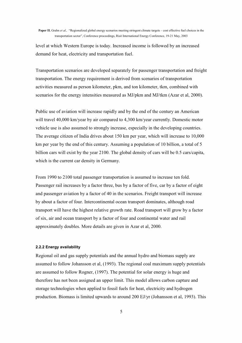
Paper II. Grahn et al., “Regionalized global energy scenarios meeting stringent climate targets – cost effective fuel choices in the
transportation sector”, Conference proceedings, Risö International Energy Conference, 19-21 May, 2003
5
level at which Western Europe is today. Increased income is followed by an increased
demand for heat, electricity and transportation fuel.
Transportation scenarios are developed separately for passenger transportation and freight
transportation. The energy requirement is derived from scenarios of transportation
activities measured as person kilometer, pkm, and ton kilometer, tkm, combined with
scenarios for the energy intensities measured as MJ/pkm and MJ/tkm (Azar et al, 2000).
Public use of aviation will increase rapidly and by the end of the century an American
will travel 40,000 km/year by air compared to 4,300 km/year currently. Domestic motor
vehicle use is also assumed to strongly increase, especially in the developing countries.
The average citizen of India drives about 150 km per year, which will increase to 10,000
km per year by the end of this century. Assuming a population of 10 billion, a total of 5
billion cars will exist by the year 2100. The global density of cars will be 0.5 cars/capita,
which is the current car density in Germany.
From 1990 to 2100 total passenger transportation is assumed to increase ten fold.
Passenger rail increases by a factor three, bus by a factor of five, car by a factor of eight
and passenger aviation by a factor of 40 in the scenarios. Freight transport will increase
by about a factor of four. Intercontinental ocean transport dominates, although road
transport will have the highest relative growth rate. Road transport will grow by a factor
of six, air and ocean transport by a factor of four and continental water and rail
approximately doubles. More details are given in Azar et al, 2000.
2.2.2 Energy availability
Regional oil and gas supply potentials and the annual hydro and biomass supply are
assumed to follow Johansson et al, (1993). The regional coal maximum supply potentials
are assumed to follow Rogner, (1997). The potential for solar energy is huge and
therefore has not been assigned an upper limit. This model allows carbon capture and
storage technologies when applied to fossil fuels for heat, electricity and hydrogen
production. Biomass is limited upwards to around 200 EJ/yr (Johansson et al, 1993). This

Paper II. Grahn et al., “Regionalized global energy scenarios meeting stringent climate targets – cost effective fuel choices in the
transportation sector”, Conference proceedings, Risö International Energy Conference, 19-21 May, 2003
6
constraint has important implications since the total energy demand is much larger. Thus,
the model chooses to use biomass in the sector where it is most competitive.
Efficiency of energy conversions, cost of industrial plants, vehicle engines and fuel
infrastructure are discussed in detail in the paper presenting the global model GET 1.0
(Azar et al, 2000). The same values have been used in all regions. Regionalized load
factors for solar energy technologies give some advantages to the regions Africa, Middle
East and North Africa, Latin America and North America.
2.3 Maximum expansion constraint
It takes time to make profound changes in the energy system of the world. This inertia is
difficult to capture in energy system models. In the GET model, inertia is introduced in
several ways. First, it takes time before the capital stock is replaced and second, we have
introduced both percentage and exogenous constraints on how fast new technologies
might enter and this latter constraint is the most sensitive in GET-R 1.0, since this
maximum expansion rate can be set as a global or as a regional constraint, see Sections
2.3.1 and 2.3.2.
If a global maximum expansion rate is chosen, the model will choose to expand
technologies in regions where it is most cost-efficient, and this means that solar will
expand at a faster rate in sunnier regions than what happens if regional expansion rate
constraints are chosen. In this study we use the global maximum expansion rate as our
base case, but we will also present some interesting differences to the base case using the
other method of a regionalized maximum expansion constraint.

Paper II. Grahn et al., “Regionalized global energy scenarios meeting stringent climate targets – cost effective fuel choices in the
transportation sector”, Conference proceedings, Risö International Energy Conference, 19-21 May, 2003
7
2.3.1 Global maximum expansion rate constraint
The expansion of supply potential and the expansion of energy conversion plants are
controlled by an expansion constraint expressed as
∑ ∑ ⎟⎠⎞
⎜⎝⎛ +≤+
r rrtrt L
trMtrCtrC ),(),()1,(
where Crt(r,t) [TW] is the capital stock in a specific decade t, and a specific region r, L is
a load factor and M(r,t) is the exogenous maximum expansion rate, calculated out of the
global energy demand for each decade as
TW/decade),(),(),(),(T
trDtrDtrDtrMtrhel
α++=
where Del(r,t) [EJ/yr] is the global demand for electricity, Dh(r,t) [EJ/yr] is the global
demand for heat, Dtr(r,t) [EJ/yr] is the global demand for transport fuel and T is the
number of decades assumed to be required for the development of a completely new
energy system. Here we put T=5. The constant α=31 Ms/yr is included to account for the
conversion between GJ and TW.
2.3.2 Regional maximum expansion rate constraint
A different way of regionalizing the global maximum expansion rate is by limiting the
expansion for each technology in each region. Instead of summing over all regions the
expansion constraint is here expressed as
LtrMtrCtrC rtrt),(),()1,( +≤+
where Crt(r,t) [TW] is the accumulated capacity of capital in a specific decade t, and a
specific region r, L is a load factor and M(r,t) is the maximum expansion rate, calculated
in equation (2).
(1)
(2)
(3)
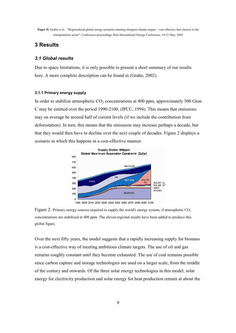
Paper II. Grahn et al., “Regionalized global energy scenarios meeting stringent climate targets – cost effective fuel choices in the
transportation sector”, Conference proceedings, Risö International Energy Conference, 19-21 May, 2003
8
3 Results
3.1 Global results
Due to space limitations, it is only possible to present a short summary of our results
here. A more complete description can be found in (Grahn, 2002).
3.1.1 Primary energy supply
In order to stabilize atmospheric CO2 concentrations at 400 ppm, approximately 500 Gton
C may be emitted over the period 1990-2100, (IPCC, 1994). This means that emissions
may on average be around half of current levels (if we include the contribution from
deforestation). In turn, this means that the emissions may increase perhaps a decade, but
that they would then have to decline over the next couple of decades. Figure 2 displays a
scenario in which this happens in a cost-effective manner.
Figure 2: Primary energy sources required to supply the world's energy system, if atmospheric CO2
concentrations are stabilized at 400 ppm. The eleven regional results have been added to produce this
global figure.
Over the next fifty years, the model suggests that a rapidly increasing supply for biomass
is a cost-effective way of meeting ambitious climate targets. The use of oil and gas
remains roughly constant until they become exhausted. The use of coal remains possible
since carbon capture and storage technologies are used on a larger scale, from the middle
of the century and onwards. Of the three solar energy technologies in this model, solar
energy for electricity production and solar energy for heat production remain at about the

Paper II. Grahn et al., “Regionalized global energy scenarios meeting stringent climate targets – cost effective fuel choices in the
transportation sector”, Conference proceedings, Risö International Energy Conference, 19-21 May, 2003
9
same level as wind and hydro, but solar energy for hydrogen production increases rapidly
during the second half of the century.
3.1.2 Transportation
The scenario describing the cost-effective fuel choices in the transportation sector is
presented in Figure 3.
Figure 3: Projected transportation fuels requirements, if atmospheric CO2 concentrations are stabilized at
400 ppm. Note that regional results are added to give a global figure.
In cars and freight sectors there is a transition from petroleum-based fuels in internal
combustion engines to hydrogen used in fuel cell engines. Some methanol in internal
combustion engines will be used in the transition period in both sectors. The model also
present natural gas as a cost-effective transition fuel in the sector cars. In airplanes, there
is a transition from fuels based on oil towards liquefied hydrogen.
3.1.3 Heat and electricity production
The end-use sector heat is defined as the heat required domestically as well as process heat
in industries. The regional results, showing the scenarios for heat and electricity
production, are added to give the global figures presented in Figure 4.

Paper II. Grahn et al., “Regionalized global energy scenarios meeting stringent climate targets – cost effective fuel choices in the
transportation sector”, Conference proceedings, Risö International Energy Conference, 19-21 May, 2003
10
Figure 4: Primary energy sources used to supply households and industries global demand for heat as
well as primary energy sources to supply the world's demand of electricity, given that atmospheric CO2
concentrations are stabilized at 400 ppm. These graphs are produced using the global maximum expansion
constraint and regional results are added together.
Biomass and coal dominate as primary energy source for heat production. For electricity
production oil is phased out early and by the end of the century coal increases due to the
fact that decarbonization techniques become cost-effective and used on a larger scale.
When solar based hydrogen is introduced by the middle of the century it will rapidly
increase its share and dominate as a primary energy source in year 2100. Biomass, as well
as the other renewable energy sources, displays an increasing pattern throughout the
century. Wind and hydro power are used to their exogenously set maximum level. The
decline in gas use, by the end of the century, is caused by lack of availability.
3.2 The impact of different ways of setting the maximum expansion rates
When it comes to fuel choices in the transportation sector, the difference between the two
ways of setting maximum expansion rates are minor. We will compare our two results
with the figure generated using a globally aggregated version of the model, in section 3.3
The major impact of different ways of setting the maximum expansion rates is where
solar hydrogen is being produced. Using a global maximum expansion rate, the region
Middle East and North Africa (MEA) will extract almost 200 EJ/yr of solar produced
hydrogen, in year 2100, out of which 160 EJ/yr will be exported to other regions. Using a

Paper II. Grahn et al., “Regionalized global energy scenarios meeting stringent climate targets – cost effective fuel choices in the
transportation sector”, Conference proceedings, Risö International Energy Conference, 19-21 May, 2003
11
regionally set maximum expansion rate MEA will only produce solar hydrogen for its
own need. The differences in primary extraction for MEA due to choice of expansion
constraint, are illustrated in Figure 5. The Asian regions Centrally Planned Asia
dominated by China (CPA), South Asia dominated by India (SAS) and Other Pacific Asia
(PAS) are examples of regions which import hydrogen in the case of a global maximum
expansion constraint and produce their own solar hydrogen in the other case, as
illustrated in Figure 6.
Figure 5: Primary energy extracted in region Middle East and North Africa, MEA. Solar produced
hydrogen will be exported in the case of a global maximum expansion rate.
Figure 6: Primary energy sources to supply the energy demand in the Asian regions. No solar produced
hydrogen will be developed in the case of a global maximum expansion rate. Instead hydrogen will be
imported mainly from MEA. In the case of a regional maximum expansion rate the Asian regions will
produce their own solar hydrogen.

Paper II. Grahn et al., “Regionalized global energy scenarios meeting stringent climate targets – cost effective fuel choices in the
transportation sector”, Conference proceedings, Risö International Energy Conference, 19-21 May, 2003
12
3.3 The difference between a globally aggregated model and a global regionalized model
To explore if the cost-effective choice of fuel in the transportation sector will be different
if a globally aggregated model is used rather than a regionalized version, we will produce
two more figures as a comparison to Figure 3. A globally aggregated model, of this
version of the energy system model, as well as the run with regional maximum expansion
constraint, are presented in Figure 7. These two figures are very similar to Figure 3,
shown in section 3.1
Figure 7: Fuel choices in the transportation sector will show the same over all pattern no matter global or
regionalized model.
4 Discussion and conclusions In this paper, we asked the following questions: When is it cost-effective to carry out the
transition away from gasoline/diesel? To which fuel is it cost-effective to shift? Will the
cost-effective choice of fuel in the transportation sector be different if a globally
aggregated model is used rather than a regionalized version? How will the method of
regionalization affect transportation fuel choices and trade in energy carriers? Below, we
summarize our results and offer some explanations for them.

Paper II. Grahn et al., “Regionalized global energy scenarios meeting stringent climate targets – cost effective fuel choices in the
transportation sector”, Conference proceedings, Risö International Energy Conference, 19-21 May, 2003
13
4.1 Oil remains dominant in the transportation sector for several decades despite stringent climate targets
A perhaps somewhat surprising result from our modeling exercise is that oil remains
dominant in the transportation sector several decades ahead. A physical explanation for
that is that known oil and natural gas reserves, contain about 200 Gton C (and we have
assumed that the ultimately recoverable oil and natural gas resources are twice the current
reserves). It is thus possible to release more CO2 emissions than what exist in the total
reserves of oil and natural gas, and still stabilize the atmospheric CO2 concentration at
400 ppm. The most cost-effective use for oil is in the transportation sector (the
advantages of using oil in the transportation sector is larger than using oil for heat or
electricity production).
One tempting interpretation may be that no new technologies would need to be developed
until the middle of the 21st century, but other elements ensure that this is not the case. The
transition to hydrogen in the transportation sector will start around 2030 – 2050, and to
make this possible, hydrogen should be used in vehicles before 2030. It is only by 2030 –
2050 that the carbon constraint becomes stringent enough to make hydrogen and fuel cell
engines in cars and trucks competitive with gasoline and diesel.
4.2. Hydrogen and not biofuels become the dominant transportation fuel in
our model
Hydrogen becomes the dominant fuel in the transportation sector, as it is more cost-
efficient to use biomass for heat production. Using biomass to produce methanol would
imply that the heat demand would have to be satisfied from other CO2-neutral sources
(hydrogen from solar or fossil fuels with decarbonization), which would increase the
overall cost of the model. The reason why biomass can not be used for both heat and
transportation is that the overall supply is limited upwards due to availability constraints.

Paper II. Grahn et al., “Regionalized global energy scenarios meeting stringent climate targets – cost effective fuel choices in the
transportation sector”, Conference proceedings, Risö International Energy Conference, 19-21 May, 2003
14
4.3 A global but regionalized model versus a globally aggregated model
As shown in Figure 3 and in Figure 7, cost-effective choice of fuel in the transportation
sector will, more or less, not be different if a globally aggregated model is used rather
than a regionalized version. In fact many fuel choices are very close to each other in
costs, and the transition fuels is not an effect by regionalization, but an effect due to
development of the model.
4.4 Affects of the two methods of regionalization
The two methods of regionalization will not affect the overall pattern of transportation
fuel choices, but will affect the trade in energy carriers. The major impact of different
ways of setting the maximum expansion rates is where solar hydrogen is being produced,
as illustrated in Figure 5 and 6, in section 3.2.
4.5 Model results are not a prediction of the future
The purpose of this study is not to predict the future. This model illustrates which fuels
are most cost-efficient, based on presented assumptions. It is of course possible to use
this study as an indication of which fuels and technologies are most cost effective, but
even if assumptions in this model are reasonable by current standards, a great deal can
occur within the next few decades, which may change the input data and produce
different results. Also, since the model is an LP model, the less costly solution will
always be chosen completely no matter how small the difference in cost is to the closest
competing option. In reality, many options may be chosen simultaneously if the
difference in cost is minor, but this cannot happen in our model.
One general result from our study that is less dependent on the actual parameter choices
is that it is possible to combine ambitious climatic goals with an increased demand for
energy services.

Paper II. Grahn et al., “Regionalized global energy scenarios meeting stringent climate targets – cost effective fuel choices in the
transportation sector”, Conference proceedings, Risö International Energy Conference, 19-21 May, 2003
15
5 Future work The development of hybrid cars (electricity and internal combustion engine) has come to
a point when its energy efficiency is close to what is expected for a fuel cell car. This is
an important issue to follow up and include as an option in the model. In the current
version of our model, we have not included hybrid cars.
Further it could be of interest to look more into biomass supply and conversion options.
In this study biomass is a collective name for forest biomass, energy crops and biomass
residues. The end-use sector heat is a collective name for industrial process heat and
residential heating (including district heating and pellets production). If the model had
more supply and end-use options, it could maybe give a more balanced picture of the
most cost-efficient use for biomass. The use of biomass for electricity and transportation
fuel becomes more interesting, the higher the cost of using biomass for heat production.
The model could also be further developed by study the effect of more combined energy
options. The model includes co-generated electricity and heat production, but as a future
work options as for example co-generated production of methanol and heat, could be of
interest to study.
Finally, the results presented here are based on the assumption that there is a carbon
constraint applied to all regions of the world. It could be interesting to analyze fuel
choices in the transportation sector under the more realistic assumption that developing
countries will adopt abatement policies perhaps a decade or two after the industrialized
countries.
Acknowledgement We would like to acknowledge Per Kågeson for his valuable comments. Financial
support from Swedish Agency for Innovation Systems, Vinnova, and Swedish Energy
Agency is gratefully acknowledged.

Paper II. Grahn et al., “Regionalized global energy scenarios meeting stringent climate targets – cost effective fuel choices in the
transportation sector”, Conference proceedings, Risö International Energy Conference, 19-21 May, 2003
16
References Azar C, Lindgren K, Andersson B A (2000). “Hydrogen or Methanol in the
Transportation Sector”, Department of Physical Resource Theory, Chalmers
University of Technology, Göteborg, Sweden, Report.
Azar C, Lindgren K, Andersson B A (2003). “Global energy scenarios meeting stringent
CO2 Constraints – cost-effective fuel choices in the transportation sector”, Energy
Policy 31(10), August 2003, p. 961-976.
Azar C, Rodhe H (1997). “Targets for Stabilization of Atmospheric CO2”, Science
276(5320), p. 1818-1819.
Grahn M (2002). “Global energy scenarios meeting stringent climate targets - a
comparison between the Global Energy System Model GET 1.0 and the
Regionalised Model GET-R 1.0”, MSc Thesis, Department of Physical Resource
Theory, Chalmers University of Technology, Sweden.
IPCC (1994). “Climate Change 1994 – Mitigation”, Contribution of working group III to
the third assessment report of the Intergovernmental Panel on Climate Change,
Cambridge University Press, UK.
Johansson T B, Kelly H, Reddy A K N, Williams RH (1993). Executive editor: Laurie
Burnham, “Renewable Energy – Sources for Fuels and Electricity”, Island Press,
California, USA.
Nakicenovic N, A Grubler and A McDonald (1998). “Global Energy Perspectives”.
Cambridge University Press. Scenarios from the report are also presented at
www.iiasa.ac.at/collections/IIASA_Research/Research/ECS/docs/book_st/node2.ht
ml.
Rogner H H (1997). “An Assessment of World Hydrocarbon Resources”, Annual Review
of Energy and the Environment, vol 22, p. 248.

Paper III


Paper III. Grahn et al. “Biomass for heat or transport – an exploration into the underlying cost dynamics in the GET model”, Working paper, 2006
1
Biomass for heat or transport – an exploration into the underlying cost dynamics in the GET model
Maria Grahn, Kristian Lindgren and Christian Azar Physical Resource Theory, Department of Energy and Environment, Chalmers University of Technology,
412 96 Göteborg, Sweden, E-mail: [email protected]
Abstract In earlier assessments using the global energy transition model, GET, biomass has been
found to be most cost-efficiently used for heat and to some extent power production, to
meet stringent restrictions on CO2 emissions. The aim with this study is to achieve more
detailed results on the cost dynamics in the GET model in order to get a more clear
picture on why biofuels are not seen as a cost-effective fuel choice. The analysis is
carried out in a simplified model implemented in Excel that reflects the cost data in a
further developed version of the model, GET 5.1, which has a more detailed oil and
refinery section. In the analysis, we study and compare the total cost per km for each fuel
choice, based on the primary energy prices generated by the model, and we identify the
carbon tax interval, for each time step, where biofuels have the lowest cost per km. The
simplified model explains the GET model result and gives deeper insights about the
system effect causing the result on cost-efficient fuel choices in the GET model. We find
that the required carbon tax level where biofuels become cost-efficient compared to fossil
based fuels, is evasive. The tax level moves upwards with increasing carbon tax since this
leads to an increasing biomass primary energy price in the model.
Keywords: Energy scenarios, energy systems modeling, system effect, scarcity rent,
carbon tax, primary energy price, liquid biofuels, hydrogen, carbon dioxide emissions

Paper III. Grahn et al. “Biomass for heat or transport – an exploration into the underlying cost dynamics in the GET model”, Working paper, 2006
2
1. Introduction
In order to analyze a possible future transition of the global energy system, Azar and
Lindgren have developed a global energy economy model, the GET (Global Energy
Transition) model (see e.g. Azar et al. 2000, 2003). In earlier assessments with the GET
model, biomass is found to be most cost-efficiently used for heat and to some extent
power production, to meet stringent restrictions on CO2 emissions. Biofuels1 are not seen
as a cost-effective strategy to reduce CO2 emissions.
In 2003, the European Commission proposed an increased use of biofuels in the
transportation sector in a directive which states that biofuels should constitute 2% of the
total amount of transportation fuels sold in 2005 (estimated as energy content) at the
national level, and 5.75% in the year 2010 (European Council, 2003).
In the light of this we want to further analyze why biofuels do not appear as a cost-
effective strategy to reduce carbon dioxide emissions in the GET model. The aim with
this study is to achieve more detailed results on the cost dynamics in the GET model in
order to get a deeper understanding on why biofuels are not found to be a cost-effective
fuel choice. The analysis is carried out using a further developed version of the model,
GET 5.1 and a simplified model implemented in Excel.
The paper is structured as follows: In Section 2, we describe the initial GET 1.0 model,
the new further developed model GET 5.1 and the simplified model implemented in
Excel. In Section 3 we present results of the GET 5.1 model base case set up and in
Section 4 we explain the result. In Section 5 we present a sensitivity analysis and in
Section 6 we present our conclusions.
1 In this study “biofuels” always mean transportation fuels derived from biomass.

Paper III. Grahn et al. “Biomass for heat or transport – an exploration into the underlying cost dynamics in the GET model”, Working paper, 2006
3
2. Method
To further analyze why biofuels do not appear as a cost-effective strategy to reduce
carbon dioxide emissions in the GET model (GET 5.1) we will make the analysis in two
steps. First we develop the GET model with a more detailed oil and refinery section, to
analyze if biofuels will appear as a cost-effective strategy to reduce CO2 emissions.
Secondly, to analyze the underlying cost dynamics in GET 5.1 we also develop a
simplified model implemented in Excel.
2.1 The initial GET 1.0 model
The global energy systems model, GET 1.0, is a linear programming model that is
globally aggregated and has three end-use sectors. It focuses on the transportation sector,
while the use of electricity and heat (including low and high temperature heat for the
residential, service, agricultural, and industrial sectors) are treated in a more aggregated
way. The transportation sector includes separate demands for four subgroups: Cars,
Freight, Aviation and Rail.
The model is composed of three different parts: (i) the primary energy supply with the
supply options coal, oil, natural gas, nuclear power, hydro, wind, biomass and solar
energy, (ii) the energy conversion system with plants that may convert the primary
energy supplies into secondary energy carriers, e.g., electricity, hydrogen, methanol, and
gasoline/diesel and (iii) the final energy demand which includes technologies used in the
transportation sector, see Figure 1.

Paper III. Grahn et al. “Biomass for heat or transport – an exploration into the underlying cost dynamics in the GET model”, Working paper, 2006
4
transportationsystem andtechnologies
energyconversionsystem
elec-tricity
heat
demandsupply
trans-portationmodelandscenario
CO2 CO2
biomasshydrowindsolar
nat. gasoilcoalnuclear
Fig. 1 The global energy systems model GET 1.0 is composed of three parts: supply, demand, and the
energy conversion system. The supply is characterised by annual or total extraction limits on the different
available energy sources. The demand is exogenously given for transportation, electricity, and heat
(including high temperature process heat). The technology system is characterized by a large number of
technologies available both for conversion between different energy carriers as well as for vehicle engines.
A cost minimization algorithm with restriction on emissions of fossil carbon is then applied to generate
energy scenarios.
Energy demand for electricity and heat/process heat are assumed to follow the C1
scenario developed by IIASA/WEC (Nakicenovic et al., 1998). This is one of their
“ecologically driven” scenarios in which they assume that technological development
leads to efficiency improvements, so that per capita energy demand in developed
countries is reduced. Heat/process heat is defined as all stationary use of fuels that neither
aim at generating electricity nor transportation fuels. The C1 transportation scenario is
not sufficiently detailed for the GET analysis, so a transportation scenario has been
developed by assuming that the increase in the amount of person kilometers travelled is
proportional to GDP growth (in PPP terms). Full details of the model and the demand
scenarios are available in Azar et al. (2000, 2003).
Constraints have been added to the model to avoid solutions that exhibit vary fast
changes in the energy system. This includes constraints on the maximum expansion rates
for different technologies (in general chosen so that it takes 50 years to change the entire
energy system) as well as annual or total extraction limits on the different available

Paper III. Grahn et al. “Biomass for heat or transport – an exploration into the underlying cost dynamics in the GET model”, Working paper, 2006
5
energy sources. The contribution of intermittent electricity sources is also limited to a
maximum of 30% of the electricity demand. To reflect the actual situation in developing
countries a minimum of 27 EJ/yr of the heat demand need to be produced from biomass
the first decades. The contribution of nuclear power has been constrained to the level we
have today.
We have put the global discount rate at 5% per year. Energy supply potentials, maximum
expansions rates and energy demand are exogenously given. In most cases investment
costs, conversion efficiencies, lifetimes and load factors are assumed constant at their
“mature levels”. The model can allow carbon sequestration to be applied to most fossil
fuel conversion technologies.
An optimization algorithm is applied to the model in order to generate the solution that
meets the energy demands and a specific atmospheric concentration target, with the
lowest total cost.
The energy system description in the GET model is a simplification of reality in many
ways, e.g., the number of available technologies is limited, demand is price-inelastic,
decisions in the model are only based on cost considerations, and there is no uncertainty
about future costs, climate targets or energy demand levels etc. The global energy system,
in GET, is then optimized with perfect foresight and with a single goal function, and
therefore the model is not suitable for making predictions of the energy system
development.
An energy-economy model like this is, however, useful for constructing and comparing
scenarios. The model makes it possible to quantitatively explore the role and cost-
efficiency of various technologies given different carbon emission constraints, resource
availabilities, and parameter values for technologies.

Paper III. Grahn et al. “Biomass for heat or transport – an exploration into the underlying cost dynamics in the GET model”, Working paper, 2006
6
2.2 The GET 5.1 model
There are four main new features in the GET 5.1 model, compared to GET 1.0: (i) waste
heat generated in the production of biofuels may be sold to the heat market, (ii) carbon
and capture storage technology can be applied on both biomass and fossil fuel use, (iii) a
split of the primary energy “oil” into two primary oil sources, conventional and heavy
oils and (iv) a further development of the refinery process in the model. Parameter values
are identical to those described in Azar et al. (2005) with two minor changes. First the
life times on truck engines have been shortened to 10 years instead of 15 years as in
earlier GET models, following Kågeson (2004). Secondly we have changed the energy
efficiency on fuel cells in cars, compared to internal combustion engines, from a factor of
2.2 more efficient down to a factor of 1.5, also following Kågeson (2004). Hence, a
transition into hydrogen in fuel cell vehicles is in the GET 5.1 model less favorable than
in earlier versions of the GET model.
Instead of, as in earlier GET models, one refinery process this model has two, one
conventional and one more costly, where the latter process represents the additional costs
associated with converting heavier fractions into transportation fuels. The share of
conventional and heavy oils that can go to the conventional refinery process is
maximized following rough estimates done by Wernersson (2003) and Kågeson (2004). It
is in GET 5.1 not possible to convert all oil into transportation fuels. The heaviest
fractions, 10% of the oil, may be used in the heat or electricity sectors. The new part in
the model structure is presented in Figure 2.
Fig 2. Illustration of the added new model structure in GET 5.1. The numbers to the left show the
maximum share allowed of a certain primary energy to be converted into transportation fuels using each
refinery process, e.g. a maximum of 60% of the conventional oil can be converted into transportation fuels
by the conventional refinery process and a maximum of 30% of the conventional oil can be upgraded to
transportation fuels using the more costly refinery process. Thus, at the most 90% of the oil can be
converted into transportation fuels.
Conven-tional oil
Heavy oils
Conventional refining
More costly refining
0.3
0.6
0.7
0.2
Gasoline/Diesel/ Kerosene
η=0.9
η=0.9

Paper III. Grahn et al. “Biomass for heat or transport – an exploration into the underlying cost dynamics in the GET model”, Working paper, 2006
7
The main difference with this new model structure, is that it has become more expensive
to produce oil based transportation fuels. In earlier versions of the GET model 100% of
the primary energy “oil” could be converted into transportation fuels, at a certain cost.
Now, only 60% of the conventional oil can be converted into transportation fuels, at that
cost.
The primary energy supply potentials of the two different types of oil are estimated
following Rogner (1997), EIA (2002) and WEA (2000) and in the base case set to 12,000
EJ for conventional oil and 12,000 EJ for heavy oils. The primary energy cost2 for
conventional oil is taken from the GET 5.0 model (Azar et al., 2005) and the primary
energy cost for heavy oils is estimated following EIA (2002) and in the model set to 3.5
USD/GJ3 and 5 USD/GJ respectively.
2.3 The simplified model implemented in Excel
In this study we have developed a simplified model, implemented in Excel, to explore the
underlying cost dynamics in the GET model. The parameter values and equations which
we implement in Excel are equivalent to the data and equations in the GET 5.1 model and
we calculate the costs per km for all fuel and vehicle choices.
2.3.1 Primary energy price
The primary energy price P [USD/GJ] in the GET 5.1 model, consists of three parts, as
TSRC PPPP ++= ,
2 Read more about the term “primary energy cost” in Section 2.3.1. 3 In reality, the extraction cost is only a few dollars per barrel (corresponds to 0.1-0.4 USD/GJ) in the Middle East and higher in other major oil producing regions. The price observed in the market is much higher still and reflects scarcities and the fact that oil supply is controlled by a cartell (OPEC). It would be too complicated in a model like this to simulate the price setting behaviour of a cartell. For that reason, we have chosen to set the primary energy cost, PC , (extraction cost and distribution) for conventional oil at 3.5 USD/GJ. This oil price, which prevailed towards the end of the 90s, includes the impact of the cartell's activities. When oil reserves decline the scarcity rent will increase. We get roughly the same price development for oil (P=PC+PSR) in our model even if we put the extraction cost to zero.
(1)

Paper III. Grahn et al. “Biomass for heat or transport – an exploration into the underlying cost dynamics in the GET model”, Working paper, 2006
8
where PC is the primary energy cost including the extraction costs and distribution, PSR is
a scarcity rent4 generated in the model as a shadow price for each time step and PT is the
price for emitting fossil carbon, i.e. a carbon tax.
2.3.2 Production costs of transportation fuels
Total fuel production costs CF [USD/GJ], in the GET 5.1 model, is equivalent to
DPOMIF CCCCC +++= ,
where CI is the investment cost of the energy conversion plant, COM is the operation and
maintenance cost, CP is the primary energy cost per energy output and CD is the
distribution cost to fuel stations. The investment cost CI [USD/GJ] is
( ) ( )( ) ⎟⎟
⎠
⎞⎜⎜⎝
⎛
+−−+= 10
105
1/111
101
rT
LIrCI α
,
where I [USD/kW] is the investment cost, r is the discount rate (0.05/yr in the base case),
T [yr] is the life time of the conversion plant (25 yr for fuel plants) and L is the load
factor. The constant α=31 Ms/yr is included to account for the conversion into GJ and
since one time step is ten years in GET 5.1, we put in the number of seconds for a ten
year period. The factor (1+r)5 reflects that investments are made between two time steps.
The operation and maintenance cost COM [USD/GJ] is assumed to be 4% of the
investment cost and calculated as
IL
ICOM 0018.004.0 ≈=α
,
where I [USD/kW] is the investment cost, L is the load factor, here assumed to 0.7 for all
plants and the constant α=31 Ms/yr is included to account for the conversion into GJ. The
actual operation and maintenance cost [USD] depends on the energy flow, secondary
energy, in each conversion plant and will be lower if the plant is not fully used. The cost
for the primary energy, per energy output, CP [USD/GJ] is calculated as
ηPCP = ,
4 Scarcity rent, PSR, is the economic term for the additional cost, added to the primary energy cost, PC, due to the fact that the relative price on an item increases as a result of its relatively low supply, e.g. an exhaustible resource or raw materials in high demand.
(2)
(3)
(4)
(5)

Paper III. Grahn et al. “Biomass for heat or transport – an exploration into the underlying cost dynamics in the GET model”, Working paper, 2006
9
where P [USD/GJ] is the primary energy price described in equation (1) and η is the
energy conversion efficiency. The distribution cost to fuel stations CD [USD/GJ] is
assumed to be 2 USD/GJ for gasoline and diesel, 3.5 USD/GJ for methanol and 8
USD/GJ for hydrogen, see Azar et al. (2000) for more details.
Total fuel production cost for all transportation fuel options calculated in the simplified
model, implemented in Excel, with data equivalent to the GET 5.1 base case, are
presented in Table 1.
Table 1. Assumed investment cost, conversion efficiency, conversion plant load factor, primary energy
cost, distribution cost and total fuel production cost of all transportation fuel options calculated in the
simplified model with results equivalent to GET 5.1. All costs are derived using primary energy costs PC,
i.e., without scarcity rents and carbon taxes.
Year 2000 Investment cost
I [USD/kW]
Conv.effic.
η
Load factor
L
O&M cost COM
[USD/GJ]
Primary energy cost
PC [USD/GJ]
Distribu-tion cost
CD [USD/GJ]
Tot. fuel prod. Costa)
CF [USD/GJ]
Oil Conv_Gasoline 900 0.9 0.8 1.7 3.5 2 10.3 Oil C costly_Gasoline 1300 0.9 0.8 2.4 3.5 2 12.2 Oil Heavy_Gasoline 900 0.9 0.8 1.7 5.0 2 12.0 Oil H costly_Gasoline 1300 0.9 0.8 2.4 5.0 2 13.9 Natural gas 0 1.0 1.0 0.0 2.5 6.5 8.9 Biomass_Methanol 1000 0.6 0.8 1.8 2.0 3.5 11.7 Natural gas_Methanol 600 0.7 0.8 1.1 2.5 3.5 10.0 Coal_Methanol 1000 0.6 0.8 1.8 1.0 3.5 10.0 Biomass_Hydrogen 800 0.6 0.6 1.5 2.0 8 15.9 Natural gas_Hydrogen 300 0.8 0.6 0.6 2.5 8 12.8 Coal_Hydrogen 700 0.65 0.6 1.3 1.0 8 13.5 Oil Conv_Hydrogen 400 0.75 0.8 0.7 3.5 8 14.9 Oil Heavy_Hydrogen 400 0.7 0.8 0.7 5.0 8 17.4 Solar_Hydrogen 2000 1.0 0.25 3.7 - 8 31.0 a)To be able to compare the fuel costs per vehicle, one also has to consider extra costs per vehicle, storage, fuel cells and efficiency change, see Table 3.
In Table 1 it is shown that the total fuel production costs of biomass and fossil based
methanol is similar to gasoline/diesel derived from conventional oil. It is also shown that
the production costs of natural gas, biomass and fossil based methanol are lower than
fuels based on heavy oils and lower than all hydrogen alternatives. It is, however, not
clear, from Table 1, which transportation fuel will be chosen in a cost minimization
model for two main reasons: (i) one has to consider costs for the vehicle use, e.g. extra
costs for different engine types, efficiency change and driving distances, read more in

Paper III. Grahn et al. “Biomass for heat or transport – an exploration into the underlying cost dynamics in the GET model”, Working paper, 2006
10
Section 2.3.3, and (ii) primary energy prices, P, are affected by scarcity in the model and
change over time, read more in Section 2.3.1.
2.3.3 Total costs per kilometer
On top of the production cost of energy carriers there are costs related to the vehicle use
which need to be taken into account when comparing fuel choices in the transportation
sector. The total transportation cost Ctot (t) [USD/km] for a certain vehicle and fuel is
calculated as
( ) ( ) ( )tCtECtC VFtot += ,
where CF [USD/GJ] is the total fuel production cost derived in equation (2), E(t) [GJ/km]
is the energy demand for each engine type and CV (t) [USD/km] is the vehicle cost, for a
certain time step t. The energy required for each engine type E(t) [GJ/km] is calculated as
( ) ( )δ
γ ttE = ,
where γ (t) [GJ/km] is the energy demand per km, which is assumed to decrease by time
following the used demand scenario for the transportation sector and δ is an efficiency
factor related to gasoline cars (a gasoline car is defined as 1 and a more efficient engine
type has a value larger than 1). The vehicle cost CV (t) [USD/km] is calculated as
( ) ( )( )
( )( ) ⎟⎟
⎠
⎞⎜⎜⎝
⎛
+−−+= 10
105
1/111
101
rT
tIrtCV β
,
where I [USD/vehicle] is the investment cost, r is the discount rate (0.05/yr in the base
case), T [yr] is the life time of the vehicle and β (t) [km/vehicle] is the annual driving
distance. The factor 1/10 accounts for bringing the capital cost down to an annual cost
and the factor (1+r)5 reflects that investments are made between two time steps.
Parameter values used in GET 5.1, derived values on vehicle cost CV (t), and derived
values on energy demand for each engine type E(t), are presented in Table 2.
(7)
(8)
(6)

Paper III. Grahn et al. “Biomass for heat or transport – an exploration into the underlying cost dynamics in the GET model”, Working paper, 2006
11
Table 2. Assumed investment cost on different engine types, engines life time, engines efficiency factor
compared to a gasoline car, derived energy required for each engine and derived vehicle costs, for the year
2000.
Year 2000
Investment cost I
[USD/car]
Life time T
[yr]
Engine efficiency factor δ
Energy demand E(t)
[GJ/km]
Vehicle cost CV (t) [USD/km]
Gasoline_ICa) 20000 15 1.0 0.0035 0.103 Methanol_IC 21000 15 1.0 0.0035 0.109 Natural gas_IC 21200 15 1.0 0.0035 0.110 Hydrogen_IC 22500 15 1.0 0.0035 0.116 Gasoline_FCb) 24500 15 1.3 0.0027 0.127 Methanol_FC 24500 15 1.3 0.0027 0.127 Hydrogen_FC 24000 15 1.5 0.0023 0.124 a) IC is an acronym for internal combustion engines. b) FC is an acronym for fuel cell engines.
Further, in the calculations presented here we have used a weighted global average, for
the year 2000, on a car’s annual driving distance, β (t) = 16,384 km/car and a weighted
global average, for the year 2000, on energy demand per km, γ (t) = 3.7 MJ/km. Total
cost per km for various combinations of fuel use and engine types calculated in the
simplified model, equivalent to the result in the GET 5.1 base case for the year 2000, are
presented in Table 3.
Table 3. Derived total cost [USD/km] for each fuel choice used in either an internal combustion engine or
in a fuel cell engine, equivalent to GET 5.1 results. All costs are derived using primary energy costs PC ,
i.e., without scarcity rents and carbon taxes.
Year 2000 Internal combustion engines Fuel cell engines
Total fuel cost CF
[USD/GJ]
Energy demand [GJ/km]
Fuel cost
[USD/km]
Investment cost
[USD/km]
Total cost
[USD/km]
Energy demand [GJ/km]
Fuel cost
[USD/km]
Investmentcost
[USD/km]
Total cost
[USD/km]Oil Conv_gasoline 10.29 0.0035 0.035 0.103 0.139 0.0027 0.027 0.127 0.154 Oil C_costly_gasoline 12.24 0.0035 0.042 0.103 0.146 0.0027 0.032 0.127 0.159 Oil Heavy_gasoline 11.96 0.0035 0.041 0.103 0.145 0.0027 0.032 0.127 0.158 Oil H_costly gasoline 13.91 0.0035 0.048 0.103 0.151 0.0027 0.037 0.127 0.164 Natural gas 8.90 0.0035 0.031 0.110 0.140 - - - - Biomass_methanol 11.69 0.0035 0.044 0.109 0.149 0.0027 0.031 0.127 0.158 Nat. gas_methanol 9.97 0.0035 0.034 0.109 0.143 0.0027 0.026 0.127 0.153 Coal_methanol 10.02 0.0035 0.035 0.109 0.143 0.0027 0.027 0.127 0.153 Biomass_hydrogen 15.92 0.0035 0.055 0.116 0.171 0.0023 0.037 0.124 0.161 Nat. gas_hydrogen 12.76 0.0035 0.044 0.116 0.160 0.0023 0.029 0.124 0.154 Coal_hydrogen 13.53 0.0035 0.047 0.116 0.163 0.0023 0.031 0.124 0.155 Oil Conv_hydrogen 14.89 0.0035 0.051 0.116 0.168 0.0023 0.034 0.124 0.158 Oil Heavy_hydrogen 17.37 0.0035 0.060 0.116 0.176 0.0023 0.040 0.124 0.164 Solar_hydrogen 31.04 0.0035 0.107 0.116 0.223 0.0023 0.071 0.124 0.196

Paper III. Grahn et al. “Biomass for heat or transport – an exploration into the underlying cost dynamics in the GET model”, Working paper, 2006
12
In Table 3 it is shown that the use of gasoline, produced from conventional oil, leads to
the lowest cost per km, closely followed by natural gas and thereafter natural gas and coal
based methanol, all four options used in internal combustion engines, assuming primary
energy costs, PC. Biomass based methanol used in internal combustion engines has the
lowest cost per km among the four biofuel options.
2.3.4 Production costs of electricity and heat
Total production costs C [USD/GJ] is calculated as
POMI CCCC ++= ,
where CI is the investment cost of the energy conversion plant, COM is the operation and
maintenance cost and CP is the primary energy cost per energy output. CI, COM and CP are
calculated following equation (3), (4) and (5) respectively.
Total production costs for various heat and electricity options, equivalent to the GET 5.1
base case in 2000, are calculated in the simplified model and presented in Table 4.
Table 4. Assumed investment costs, energy conversion efficiency, conversion plant load factors and
primary energy costs are listed. The total production costs for various heat and electricity options are
calculated in the simplified model, equivalent to GET 5.1. All costs are derived using primary energy costs
PC , i.e., without scarcity rents and carbon taxes.
Year 2000 InvestmentCost I
[USD/kW]
Conv.effic.
η
Load factor
L
O&M costCOM
[USD/GJ]
Primary energy cost PC [USD/GJ]
Tot. prod. cost C
[USD/GJ] Biomass_heat 300 0.9 0.7 0.6 2.0 3.8 Natural gas_heat 100 0.9 0.7 0.2 2.5 3.3 Oil Conventional_heat 100 0.9 0.7 0.2 3.5 4.4 Oil Heavy_heat 100 0.9 0.7 0.2 5.0 6.1 Coal_heat 300 0.9 0.7 0.6 1.0 2.7 Solar_heat 400 0.9 0.25 0.7 0 4.6 Solar_H2+H2_heat 2000/100 1.0/0.9 0.25/0.7 3.7/0.2 0 23.6 Biomass_electricity 1200 0.4 0.7 2.2 2.0 11.4 Natural gas_electricity 500 0.55 0.7 0.9 2.5 7.2 Oil Conv_electricity 600 0.5 0.7 1.1 3.5 10.2 Oil Heavy_electricity 600 0.45 0.7 1.1 5.0 14.3 Coal_electricity 1100 0.45 0.7 2.0 1.0 8.1 Solar_electricity 1200 1.0 0.25 2.2 0 13.9 Solar_H2+H2_electricity 2000/500 1.0/0.55 0.25/0.7 3.7/0.9 0 25.8
(9)

Paper III. Grahn et al. “Biomass for heat or transport – an exploration into the underlying cost dynamics in the GET model”, Working paper, 2006
13
In Table 4 it is shown that heat derived from coal has the lowest production cost followed
by heat derived from natural gas. The same two primary energy sources also have the
lowest production costs for electricity generation but in the opposite order where natural
gas has the lowest production cost followed by coal.
3. Results
In the base case run of the GET 5.1 model, aiming for 450 ppm, no carbon capture and
storage technology is included. Results on primary energy supply and cost-efficient fuel
choices in the transportation sector are presented in Figures 3 and 4.
Cost-efficient global primary energy supplyat base case, in GET 5.1, 450 ppm (EJ/yr)
0100200300400500600700800
2000 2010 2020 2030 2040 2050 2060 2070 2080 2090 2100
Fig 3. Cost-efficient primary energy choices to supply the global energy system, in the base case scenario
aiming for 450 ppm using the GET 5.1 model. Carbon capture and storage technology is not included. Coal
is phased out and biomass as well as solar energy play an important role. Acronyms used in the figure are:
OIL_C=conventional oil, OIL_H=unconventional heavy oils, NG=natural gas and SOLAR_H2=solar
energy stored in hydrogen.
SOLARH2
BIOMASS
OIL_C NG
COAL
NUCLEAROIL_H

Paper III. Grahn et al. “Biomass for heat or transport – an exploration into the underlying cost dynamics in the GET model”, Working paper, 2006
14
Cost-efficient global transportation fuelsat base case, in GET 5.1, 450 ppm (EJ/yr)
0
50
100
150
200
250
300
2000 2010 2020 2030 2040 2050 2060 2070 2080 2090 2100
Fuel choices in subgroup Cars only (EJ/yr)
0
10
20
30
40
5060
70
80
90
100
2000 2010 2020 2030 2040 2050 2060 2070 2080 2090 2100
Fig 4. Cost-efficient transportation fuels, in the base case scenario, aiming for 450 ppm, using the GET 5.1
model. Oil based transportation fuels dominate until natural gas enters the transportation sector by the year
2030 and solar based hydrogen by the year 2060. Biofuels do not appear as a cost-effective fuel choice in
this scenario. Figure 4a shows the fuel choices for the whole transportation sector where the three
subgroups: Cars, Freight and Aviation are aggregated. Figure 4b shows the fuel choices for subgroup Cars
only. Acronyms used in the figure are: OIL_C= conventional oil, OIL_H= gasoline, diesel and kerosene
produced from unconventional heavy oils, IC= internal combustion engines and FC= fuel cell engines.
In this run of the GET 5.1 model, the same overall results as in previous GET model
studies appear, i.e. that gasoline/diesel remain for some decades in the transportation
sector until the carbon constraint becomes increasingly stringent and that solar based
hydrogen dominates by the end of this century. One significant exception from previous
GET model results is, however, that natural gas has taken a larger share of the
transportation fuels, which is a result of that only 60% of the conventional oil can be
converted to gasoline and diesel at conventional refinery cost, in the GET 5.1 model,
compared to 100% in earlier GET versions, see Figure 2 and Table 3.
GASOLINE DIESEL in IC from OIL_C
NATURAL GAS in IC
SOLAR HYDROGEN
in FC
Fuel choices in subgroup Cars only (EJ/yr)
b)
TRAIN ELECTRICITY
GASOLINE DIESEL KEROSENE from OIL_C NATURAL GAS
HYDROGEN
OIL_H
a)

Paper III. Grahn et al. “Biomass for heat or transport – an exploration into the underlying cost dynamics in the GET model”, Working paper, 2006
15
4. Explaining the result
In this section we attempt to shed light on fuel choices for the subgroup Cars in the
transportation sector, by using results from the simplified model, implemented in Excel.
4.1 Total costs per kilometer as a function of carbon tax
We use equation (6) to calculate the total costs [USD/km] in the simplified model (see
Table 3). These costs are then plotted as a function of the carbon tax [USD/tC] to
illustrate how the relation between the costs change with higher carbon taxes, i.e that
carbon taxes make it more expensive to use coal, oil and natural gas, see Figure 5. Note
that these costs are derived using primary energy costs, PC, i.e., without scarcity rents. If
the full GET model were run with high carbon taxes, scarcity rents would arise, but these
rents are not included in Figure 5.
Cost per km (fuel+infrastructure+vehicle) as a function of carbon tax, for subgroup Cars
0.135
0.137
0.139
0.141
0.143
0.145
0.147
0.149
0.151
0.153
0 20 40 60 80 100 120 140 160 180 200 220 240
USD/tC
USD
/km
Fig 5. Costs per km as a function of carbon tax for subgroup Cars. Note that these costs are based on
primary energy costs PC , presented in Table 1, and not affected by scarcity. Conventional oil has the lowest
cost per km in the carbon tax interval 0-58 USD/tC, natural gas in the interval 58-160 USD/tC and biomass
based methanol in the interval 160-∞ USD/tC. Acronyms used in the figure are: OIL_C= conventional oil,
NG= natural gas, MEOH= methanol and IC= internal combustion engines.
COAL-MEOH_IC
NG_IC
OIL_C_IC
BIO-MEOH_IC
NG-MEOH_IC

Paper III. Grahn et al. “Biomass for heat or transport – an exploration into the underlying cost dynamics in the GET model”, Working paper, 2006
16
In Figure 5 it is shown that cars run on gasoline and diesel from conventional oil have the
lowest cost per km at carbon taxes up to 58 USD/tC. At taxes between 58 and 160
USD/tC natural gas cars have the lowest cost per km and at taxes above 160 USD/tC cars
run on biomass based methanol have the lowest cost per km. The figure illustrates how
the costs per km change by increasing carbon tax, using primary energy costs PC.
However, in the GET model scarcity rents, obtained from shadow prices on the primary
energy supply equation, are generated for each time step. In the base case run of the GET
5.1 model scarcity rents are generated on natural gas, conventional oil and biomass5.
In Figure 6, the costs per km generated in the base case run of the GET 5.1 model are
presented for four time steps. The graphs show how the cost per km for different fuel
choices would change with the carbon tax, given the primary energy price, P, (minus PT)
generated by the model for each time step, i.e. scarcity rents generated in the run for a
specific time step are kept constant6 in each plot. Plots for time steps 2030, 2050, 2070
and 2090 are presented in Figure 6. The vertical dotted line in each graph marks the
generated carbon tax for the specific time step.
5 Scarcity rents are generated on biomass due to the fact that the demand for biomass exceeds the supply potential at high carbon taxes. When the model is run without restrictions on CO2 emissions, no scarcity rent is added to the biomass primary energy cost. 6 Note that if the GET model were run with higher carbon taxes, scarcity rents on biomass would increase as a consequence of an even stronger competition for biomass. Thus, it is not possible to foresee any other GET results outside the point of intersection with the dotted vertical carbon tax curve.

Paper III. Grahn et al. “Biomass for heat or transport – an exploration into the underlying cost dynamics in the GET model”, Working paper, 2006
17
Cost per km (fuel+infrastructure+vehicle) as a function of carbon tax in the year 2030
0.140
0.142
0.144
0.146
0.148
0.150
0.152
0.154
0.156
0.158
0 25 50 75 100 125 150 175 200 225 250 275 300
USD/tC
USD
/km
Cost per km (fuel+infrastructure+vehicle) as a function of carbon tax in the year 2050
0.145
0.150
0.155
0.160
0.165
0.170
0 50 100 150 200 250 300 350 400 450 500 550 600
USD/tC
USD
/km
Cost per km (fuel+infrastructure+vehicle)
as a function of carbon tax in the year 2070
0.150
0.160
0.170
0.180
0.190
0.200
0 100 200 300 400 500 600 700 800 900 1000 1100 1200
USD/tC
USD
/km
Cost per km (fuel+infrastructure+vehicle) as a function of carbon tax in the year 2090
0.150
0.160
0.170
0.180
0.190
0.200
0.210
0 140 280 420 560 700 840 980 1120 1260 1400 1540 1680
USD/tC
USD
/km
Fig 6. Costs per km (subgroup Cars only) generated in the base case set up, aiming for 450 ppm, of the
GET 5.1 model. Graphs for the time steps 2030, 2050, 2070 and 2090 are presented and the vertical dotted
line marks the generated carbon tax, which is in a) 52 USD/tC, b) 157 USD/tC, c) 490 USD/tC and d) 1673
USD/tC. Note that the scarcity rents generated in each time step are kept constant in each plot. Acronyms
used in the figure are: OIL_C= conventional oil, OIL_H= heavy oils, NG= natural gas, MEOH= methanol,
H2= hydrogen, IC= internal combustion engines and FC= fuel cell engines.
In Figure 6 it is shown that in the year 2030 (a) and the year 2050 (b) cars run on gasoline
and diesel from conventional oil lead to the lowest cost per km at carbon taxes up to (a)
80 USD/tC and (b) 160 USD/tC. For carbon taxes in the interval of (a) 80-150 USD/tC
and (b) 160-350 USD/tC natural gas cars have the lowest cost per km and at carbon taxes
above (a) 150 USD/tC and (b) 350 USD/tC cars run on biomass based methanol have the
lowest cost per km.
COAL-MEOH_IC
NG_IC
OIL_C_IC
BIO-MEOH_ICOIL_H_IC
b)
COAL-MEOH_IC
NG_IC
OIL_C_IC
SOLAR-H2_FC
OIL_H_IC
BIO-H2_FC
c)
BIO-MEOH_IC
COAL-MEOH_IC
NG_IC
OIL_C_IC
SOLAR-H2_FC
OIL_H_IC
d)
SOLAR-H2_IC
a)
COAL-MEOH_IC
NG_IC
OIL_C_IC
BIO-MEOH_IC
NG-MEOH_IC

Paper III. Grahn et al. “Biomass for heat or transport – an exploration into the underlying cost dynamics in the GET model”, Working paper, 2006
18
In Figure 6c it is shown that in the year 2070 cars run on coal based methanol have the
lowest cost per km up to 25 USD/tC. For carbon taxes in the interval of 25-410 USD/tC
cars run on gasoline and diesel derived from heavy oils have the lowest cost per km and
for taxes between 410-950 USD/tC natural gas cars have the lowest cost per km and at
carbon taxes above 950 USD/tC cars run on biomass based methanol have the lowest cost
per km. Note that two other carbon neutral alternatives are close to biomass based
methanol in the year 2070, i.e. solar based hydrogen in fuel cell vehicles and biomass
based hydrogen in fuel cell vehicles.
In Figure 6d it is shown that in the year 2090 cars run on coal based methanol have the
lowest cost per km up to 25 USD/tC. For taxes in the interval of 25-930 USD/tC cars run
on gasoline and diesel derived from heavy oils have the lowest cost per km and for taxes
above 930 USD/tC cars run on solar based hydrogen in fuel cell vehicles have the lowest
cost per km. Note that the cost per km on biomass based methanol now is higher than
solar based hydrogen, which is due to a high scarcity rent on biomass (the generated
primary energy price, P, on biomass is 37 USD/GJ in the year 2090). The costs per km,
in the year 2090, for the six carbon-neutral alternatives are presented in Table 5.
Table 5. Generated total costs [USD/km] for the six fossil carbon-neutral alternatives in the GET 5.1
model, for the year 2090. The costs are based on the generated primary energy price, P, i.e. include scarcity
rent on biomass.
Year 2090 Internal combustion engines [USD/km] Fuel cell engines [USD/km] Biomass_methanol 0.263 0.256 Biomass_hydrogen 0.281 0.245 Solar_hydrogen 0.201 0.192
In Table 5 it is shown that biomass based alternatives have received a higher cost per km
compared to solar based alternatives. Note that the cost per km is lower if the fuels are
used in fuel cell engines compared to internal combustion engines. This is a result of that
a smaller amount of the relatively expensive primary energy is needed to drive one
kilometer using fuel cell engines since they are more energy efficient than internal
combustion engines.

Paper III. Grahn et al. “Biomass for heat or transport – an exploration into the underlying cost dynamics in the GET model”, Working paper, 2006
19
4.2 Fuel choices for different carbon taxes
The intervals where a certain fuel has the lowest cost per km are identified for each time
step, by analyzing the plots presented in Figure 6. Note that the scarcity rents generated
in the model run are kept constant7 in each of the analyzed plots. The identified intervals
for each time step are summarized in Figure 7, where also the carbon tax generated in the
GET 5.1 base case is plotted.
Cost-efficient fuel choices at different CO2-taxes
0
500
1000
1500
2000
2500
3000
3500
2000 2010 2020 2030 2040 2050 2060 2070 2080 2090 2100
Fig 7. Fuel choices in the transportation sector (subgroup Cars only) for different carbon tax intervals in
the base case scenario, aiming for 450 ppm. For each time step the lowest fuel cost per km for a certain
range of carbon taxes are identified and plotted in bars. The carbon tax generated in the run is plotted as a
line curve in front of the bars, with the tax values marked with x. The fuel range that crosses the carbon tax
line curve will first and foremost be chosen in the scenario. Acronyms used in the figure are: OIL_C=
conventional oil, OIL_H= unconventional heavy oils, MEOH= methanol and SOLAR-H2= solar based
hydrogen.
7 Read more in Section 4.1
Fuel choices for different CO2 taxes
BIO
-MEO
H
BIO
-MEO
H
BIO
-MEO
H
BIO
-MEO
H
BIO
-MEO
H
SOLA
R-H
2
BIO
-MEO
H
BIO
-MEO
H
OIL_H
OIL_H
SO
LAR
-H2
SOLA
R-H
2
SOLA
R-H
2 O
IL_H
USD/tC
CO2 TAX IN GET 5.1
OIL_H
NATURAL GAS
OIL_C
OIL_C COAL-MEOH

Paper III. Grahn et al. “Biomass for heat or transport – an exploration into the underlying cost dynamics in the GET model”, Working paper, 2006
20
In a linear optimization model the technology and fuel choice which offers the lowest
cost per km will first and foremost be chosen (when primary energy prices include
scarcity rents from competition with other end uses), but since the model has expansion
rate constraints a technology might enter some time steps earlier to be able to expand into
large volumes. This is the case with solar based hydrogen, which enters the scenario in
2060-2070, see Figure 4b, but crosses the carbon tax line curve, in Figure 7, first in the
year 2080. The model also has constraints on the rate of which a fuel can be phased out
which, together with the fact that capital decays exponentially, explains why
conventional oil remains in the transportation sector for some decades, see Figure 4b,
even though natural gas crosses the carbon tax line curve in the years between 2040 to
2080, in Figure 7. The reason for the increasing use of gasoline and diesel derived from
conventional oil in the years 2060 and 2070, in the scenario for subgroup Cars, is that
investments are made in new refinery capacity to supply the Freight and the Aviation
sector. Using some of the capacity to produce gasoline/diesel for cars will lower the total
energy system cost, but that can not be seen in Figure 7.
4.3 The system effect
The fuel choices in the transportation sector depend highly on fuel choices in the heat and
the electricity sector, i.e. a system effect. By studying Figure 7 it would be tempting to
interpret the carbon tax intervals as biofuels would become a cost-effective fuel choice if
the carbon tax would be higher than 150 USD/tC in the year 2030, but this can not be
taken for granted. A run where the carbon tax is locked to 160 USD/tC for the years
2010-2030, does not introduce any biofuels. Instead, the primary energy price, P, on
biomass increases to 4.4 USD/GJ compared to 2.3 USD/GJ in the base case. The
increased primary energy price on biomass is a result of an increased demand for CO2-
neutral energy in all three sectors, when the carbon tax is raised. The higher cost on
biomass increase the cost on biomass based methanol to 0.161 USD/km compared to
0.151 USD/km in the base case, while the cost per km for the fossil fuel options, when
the carbon tax is subtracted, are roughly the same, see Figures 6a and 8a.

Paper III. Grahn et al. “Biomass for heat or transport – an exploration into the underlying cost dynamics in the GET model”, Working paper, 2006
21
Cost per km (fuel+infrastructure+vehicle) as a function of carbon tax in the year 2030
0.140
0.145
0.150
0.155
0.160
0.165
0 35 70 105 140 175 210 245 280 315 350 385 420
USD/tC
USD
/km
Cost per km (fuel+infrastructure+vehicle) as a function of carbon tax in the year 2030
0.140
0.150
0.160
0.170
0.180
0.190
0.200
0 90 180 270 360 450 540 630 720 810 900 990 1080
USD/tC
USD
/km
Fig 8. Costs per km (subgroup Cars only) generated in two runs with fixed carbon taxes on a) 160 USD/tC
for the years 2010-2030 and b) 400 USD/tC for the years 2010-2050. Both scenarios reach 450 ppm by the
year 2100. Cars run on gasoline and diesel, from conventional oil, have the lowest cost per km at carbon
taxes up to a) 140 USD/tC and b) 260 USD/tC. For carbon taxes in the interval of a) 140-340 USD/tC and
b) 260-990 USD/tC natural gas cars have the lowest cost per km and for carbon taxes above a) 340 USD/tC
and b) 990 USD/tC cars run on biomass based methanol have the lowest cost per km. Thus, biomass based
methanol has a higher cost per km in these two runs compared to the base case, presented in Figure 6a.
Even though the carbon tax is increased to a level where biofuels seemed to be cost-
effective in Figure 7, the same fuel choices appear in Figure 6a as in 8a with the
difference that biomass based methanol has a higher cost per km in Figure 8a. Instead of
having the lowest cost of all fuel choices at taxes above 150 USD/tC, biomass based
methanol now has the lowest cost per km at taxes above 340 USD/tC. Increasing the
carbon tax to 400 USD/tC for the years 2010-2050 will still not introduce any biofuels,
see Figure 8b. In this run the competition, between biomass based heat and biofuels, is
strong and the primary energy price, P, on biomass has increased to 10.7 USD/GJ leading
to a cost of biomass based methanol of 0.190 USD/km. In this run it seems that biomass
based methanol will not be able to compete until the carbon tax is above 990 USD/tC.
This evasive carbon tax level when biofuels become cost-efficient, compared to fossil
based fuels, is an effect of the system effect. The tax level moves upwards with
increasing carbon taxes, since this leads to an increasing biomass primary energy price, P,
in the model.
a)
COAL-MEOH_IC
NG_IC
OIL_C_IC
BIO-MEOH_IC
NG-MEOH_IC
b)
COAL-MEOH_IC
NG_IC
OIL_C_IC
BIO-MEOH_IC
NG-MEOH_IC

Paper III. Grahn et al. “Biomass for heat or transport – an exploration into the underlying cost dynamics in the GET model”, Working paper, 2006
22
Biofuels are not introduced in the transportation sector since biomass is more cost-
effectively used in other sectors. This can also be understood by studying Table 3 and
Table 4 where the costs for the two competing CO2-neutral energy options (solar and
biomass) can be compared. In the transportation sector, by going from biomass based
methanol in internal combustion engines (0.149 USD/km) to solar based hydrogen in fuel
cells (0.196 USD/km), we get an increase of the cost per km by a factor of 1.3. In the
electricity sector by going from biomass based electricity (11.4 USD/GJ) to electricity
derived from solar based hydrogen (25.8 USD/GJ) we get an increase of the cost per
Joule by a factor of 2.3. In the heat sector by going from biomass based heat (3.82
USD/GJ) to heat derived from solar based hydrogen (23.6 USD/GJ) we get an increase of
the cost per Joule by as much as a factor of 6.2. Hence biofuels are not introduced in the
transportation sector since biomass is most cost-effectively used in the heat sector.
5. Sensitivity analysis
As explained in Section 4, the system effect in the GET 5.1 model prioritizes the limited
biomass to the heat sector. This indicates that a situation in which biofuels enter the
transportation sector should involve other types of changes to the model, for example,
other cost assumptions, features, and/or constraints. To analyze under what circumstances
biofuels could become a cost-effective strategy to reduce CO2 emissions, we have carried
out a sensitivity analysis with respect to parameter values in the GET 5.1 model as
follows. We investigate how the fuel choices in the transportation sector change if we
1) assume a lower conventional oil supply potential. We have chosen to decrease the
conventional oil reserves into 9,000 EJ and increase the heavy oils reserves into
15,000 EJ (Compared to base case 12,000 EJ each).
2) assume that waste heat generated in the production of transportation fuels may be
sold to the heat market. We introduce co-generation of methanol and heat as well
as hydrogen and heat, to the model.
3) assume a larger biomass supply potential. We have chosen to increase the supply
potential from 200 EJ to 300 EJ/yr.

Paper III. Grahn et al. “Biomass for heat or transport – an exploration into the underlying cost dynamics in the GET model”, Working paper, 2006
23
4) assume that 25% of all biomass used for heat production needs to be refined, e.g.
using wood pellets instead of using wood chips for the production of bio-heat. We
have chosen to add 3 USD/GJ for the refining process which increases the
production cost for heat produced from wood pellets into 6.82 USD/GJ (compared
to heat produced from standard wood chips 3.82 USD/GJ) following Andersson et
al. (2003).
5) assume that carbon capture and storage technology can be applied on both
biomass and fossil fuels.
We have observed that change number 3 (increasing the biomass supply potential) has a
positive effect8 on biofuel use and that change number 1 (lowering conventional oil
supply potential) has a small positive effect. Also change number 2 (including co-
generation of transportation fuels and heat) has a positive effect, but assuming that waste
heat generated in the transportation fuel production does not only have a positive effect
on biomass based methanol but also on fossil based methanol.
Change number 4 (assuming that 25% of all biomass based heat needs to be refined)
generally shows no effect on the production of biofuels. The higher production cost on
biomass based heat leads to that a smaller amount of biomass is used in the heat sector. In
early decades, when the CO2 constraint is moderate, more fossil fuels are possible to use.
Biomass based heat is replaced by coal based heat and the surplus biomass is used in the
electricity sector and generally not in the transportation sector. Change 4, however, has a
positive effect on biofuel production when it is combined with change 2 where biofuels
replace most of the fossil based methanol, see Figure 9.
Change number 5 (including carbon and capture storage technology) has a negative effect
on biofuel production. The use of coal increases as a result of including carbon and
capture storage technology. Coal replaces, to some extent, natural gas in the electricity
sector and the surplus natural gas replaces biofuels in the transportation sector. Also some
coal based hydrogen enters the transportation sector and replaces bio-methanol.
8 “Positive effect on biofuel use” means an increased share of biofuels in the transportation fuel scenario.

Paper III. Grahn et al. “Biomass for heat or transport – an exploration into the underlying cost dynamics in the GET model”, Working paper, 2006
24
Changes 1, 2 and 3 are combined to generate Figure 9a and changes 1, 2, 3 and 4 are
combined to generate Figure 9b.
Cost-efficient global transportation fuelsusing the GET 5.1 model, 450 ppm (EJ/yr)
0
50
100
150
200
250
300
2000 2010 2020 2030 2040 2050 2060 2070 2080 2090 2100
Cost-efficient global transportation fuelsusing the GET 5.1 model, 450 ppm (EJ/yr)
0
50
100
150
200
250
300
2000 2010 2020 2030 2040 2050 2060 2070 2080 2090 2100
Fig 9. Cost-efficient fuel choices in the transportation sector in two runs with a) changes 1, 2 and 3
combined and b) changes 1, 2, 3 and 4 combined. In these runs biofuels account for a) 12% and b) 44% of
total transportation fuels in the year 2050. Both runs reach 450 ppm by year 2100. Acronyms used in the
figure are OIL_C= conventional oil, OIL_H= unconventional heavy oils, FOSS-MEOH= methanol derived
from fossil fuels and BIO-MEOH= biomass based methanol.
It is shown that the use of biofuels is a cost-effective strategy to reduce CO2 emissions, if
we assume a lower conventional oil supply potential, a larger biomass supply potential,
that waste heat generated in the production of transportation fuels may be sold to the heat
market and that 25% of all biomass used for heat production need to be refined. In Figure
9b, a large amount of biofuels, accounting for 44% of total transportation fuel production
by the year 2050, is used.
6. Conclusions
Cost-effective fuel choices generated in the GET model are first and foremost a result of
a system effect. Biofuels do not appear as a cost-effective fuel choice since that would
imply that hydrogen from solar energy would be necessary to satisfy the demand for heat
(to be able to reach ambitious CO2 concentration levels). This is, using our technology
cost parameters, more costly than using biomass for the heat sector and using the
TRAIN ELECTRICITY
OIL_C
NATURAL GAS HYDROGEN
OIL_H
a)
BIO-MEOH
FOSS-MEOH
TRAIN ELECTRICITY
OIL_C
NATURAL GAS HYDROGEN
OIL_H
b)
BIO-MEOH
FOSS-MEOH

Paper III. Grahn et al. “Biomass for heat or transport – an exploration into the underlying cost dynamics in the GET model”, Working paper, 2006
25
hydrogen in the transportation sector. For that reason, hydrogen from solar becomes the
cost-efficient fuel choice in the long run also in the GET 5.1 model transportation sector.
In this study, we have developed a method, implemented in Excel, which explains the
GET model result and gives deeper insights about the system effect. By studying the cost
dynamics in the GET model, i.e. comparing the generated total costs per km for each fuel
choice and identify the carbon tax intervals for each time step where biofuels have the
lowest cost per km, we find that the required carbon tax level where biofuels become
cost-efficient compared to fossil based fuels, is evasive. The tax level moves upwards
with increasing carbon taxes, since this leads to an increasing biomass primary energy
price in the model.
In the sensitivity analysis we find that the model is sensitive for some type of changes. If
we assume a lower conventional oil supply potential, a larger biomass supply potential,
that waste heat generated in the production of transportation fuels may be sold to the heat
market and that 25% of all biomass used for heat production need to be refined, and
combine these four assumptions, a large amount of biofuels will enter the transportation
fuel scenario. In a future work we will, however, continue the sensitivity analysis and
also look deeper into how reasonable these new assumptions are and analyze possible
barriers for introducing them.
Acknowledgement
Financial support from Swedish Agency for Innovation Systems, Vinnova, and Swedish
Energy Agency is gratefully acknowledged.

Paper III. Grahn et al. “Biomass for heat or transport – an exploration into the underlying cost dynamics in the GET model”, Working paper, 2006
26
References
Andersson E, A Frimanzon and A Vidlund (2003). “Energieffektiv biobränsleförädling i
skogsindustrin” (in Swedish), Arbetsnotat Nr 24, Chalmers University of
Technology, ISSN 1403-8307.
Azar C, K Lindgren and B A Andersson (2000). “Hydrogen or methanol in the
transportation sector?”, Department of Physical Resource Theory, Chalmers
University of Technology, Göteborg, Sweden.
Azar C, K Lindgren and B A Andersson (2003). “Global energy scenarios meeting
stringent CO2 constraints - cost-effective fuel choices in the transportation sector”,
Energy Policy 31(10), 961–976.
Azar C, K Lindgren, E Larson, and K Möllersten (2005). “Carbon capture and storage
from fossil fuels and biomass - costs and potential role in stabilizing the
atmosphere”, Climatic Change, (in press).
EIA (2002). “International Energy Outlook, 2002”, Energy Information Administration –
Official Energy statistiscs from the U.S. Government, World resources,
Washington, USA, Available at www.eia.doe.gov
European Council (2003). “Directive 2003/30/EC of the European parliament and of the
council of 8 may 2003 on the promotion of the use of biofuels or other renewable
fuels for transport”, Official Journal of the European Union, L 123/42, 17.5.2003.
Available at
http://europa.eu.int/comm/energy/res/legislation/doc/biofuels/en_final.pdf.
Kågeson Per (2004). Nature Associates, Stockholm, Sweden. Personal communication,
19 Jan 2004.

Paper III. Grahn et al. “Biomass for heat or transport – an exploration into the underlying cost dynamics in the GET model”, Working paper, 2006
27
Nakicenovic N, A Grubler and A McDonald (1998). “Global Energy Perspectives”.
Cambridge University Press. Scenarios from the report are also presented at
www.iiasa.ac.at/collections/IIASA_Research/Research/ECS/docs/book_st/node2.ht
ml.
Rogner H H (1997). “An assessment of world hydrocarbon resources”, Annual Review of
Energy and the Environment, vol 22, p. 248, 1997.
WEA (2000). “World Energy Assessment”: Energy and the challenge of sustainability.
UNDP, New York. Available at http://www.undp.org/seed/eap/activities/wea/
Wernersson Clas (2003). Senior Process Engineer, Shell Raffinaderi AB, Göteborg,
Sweden. Personal communication, 23 Jan 2003.