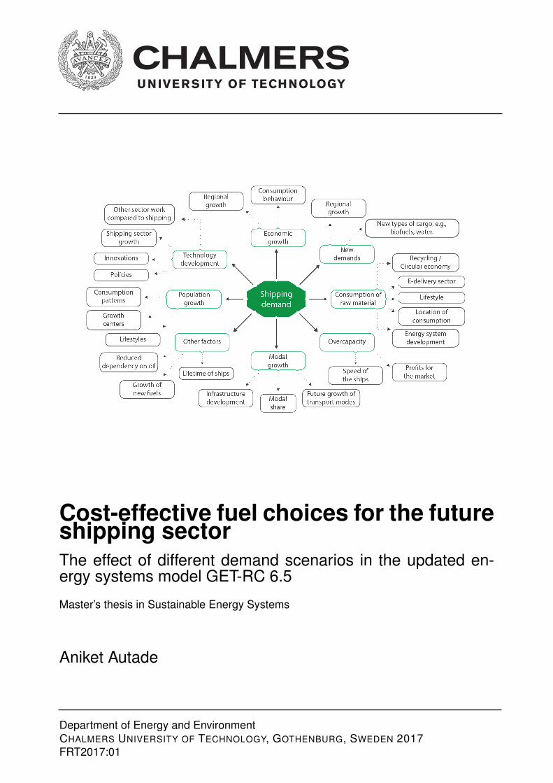
Cost-effective fuel choices for the futureshipping sectorThe effect of different demand scenarios in the updated en-ergy systems model GET-RC 6.5

Master’s thesis in Sustainable Energy Systems

Aniket Autade

Department of Energy and EnvironmentCHALMERS UNIVERSITY OF TECHNOLOGY, GOTHENBURG, SWEDEN 2017FRT2017:01

ii

FRT2017:01

Cost-effective fuel choices for the future shipping sector:the effect of different demand scenarios in the updated

energy systems model GET-RC 6.5

Aniket Autade

Department of Energy and EnvironmentDivison of Physical Resource Theory

CHALMERS UNIVERSITY OF TECHNOLOGY

Gothenburg, Sweden 2017

Cost-effective fuel choices for the future shipping sector: the effect of different demandscenarios in the updated energy systems model GET-RC 6.5

Aniket Autade

© Aniket Autade, 2017.

Supervisor:Julia Hansson, IVL Swedish Environmental Research Institute, Stockholm, SwedenMaria Grahn, Divison of Physical Resource Theory, Chalmers University of Technology,SwedenExaminer:Maria Grahn, Divison of Physical Resource Theory, Chalmers University of Technology,Sweden

Master’s Thesis FRT2017:01Department of Energy and EnvironmentDivison of Physical Resource TheoryChalmers University of TechnologySE-412 96 GothenburgTelephone +46 31 772 1000

Cover: Factors affecting shipping demand while reducing GHG emissions © Aniket Au-tade, 2017.

Typeset in LATEXPrinted by Chalmers University of TechnologyGothenburg, Sweden 2017

iv

Cost-effective fuel choices for the future shipping sector: the effect of different demandscenarios in the updated energy systems model GET-RC 6.5

Aniket AutadeDepartment of Energy and EnvironmentChalmers University of Technology

AbstractThe impacts of climate change are a complex area. To avoid known as well as unknownimpacts, there is a need to make transition towards non-GHG emitting energy system.Shipping transport sector, a part of global energy system, corresponds to 3.1% of globalanthropogenic CO2 emissions for the period 2007-2013. The aim of this thesis is to de-velop demand scenarios for the future shipping sector and evaluate the impact of demandscenarios on the cost-effective fuel choices in a carbon constrained world for the timeperiod 2010-2100. The aim is further to deepening the understanding around what carbontax that may be needed to fulfill the fuel scenarios. The purpose is to provide input todifferent shipping stakeholders and policy makers aimed at designing pathways for sus-tainable development in the shipping sector. Multi-variable linear function of shippingdemand in terms of population and economic growth (in terms of GDP) has been estab-lished using regression analysis to calculate shipping demand until the year 2100. SSP2scenario has been incorporated in Global Energy Transition (GET-RC 6.5) model. Notonly the GET-RC 6.5 model became consistent with all demands from every sector butthe shipping demand is calculated using population and economic growth values takenfrom IIASA database. This study is performed using the GET-RC 6.5 model which is aglobal linear progammed energy systems model and provides results over cost-effectivefuel choices. The results obtained during this masters thesis include: 1) The cost-effectivechoices in a 400 ppm CO2 concentration scenario suggest LNG as transitional fuel andhydrogen as the longer term alternative marine fuel for the shipping sector. 2) The level ofshipping demand is very vital for the use of fuel cell technology coupled with hydrogenspecifically for the shipping sector. 3) In case where hydrogen is not available as ship-ping fuel, the use of petrol based fuel(HFO/MGO) increases, alongside with the small butsignificant use of biofuels and electrofuels with fuel cells. 4) The role of natural gas be-comes even more vital for the shipping sector if hydrogen is assumed not to be a shippingfuel. 5) The needed tax level for generating similar incentives as in a 400 ppm scenarioand IMO discussed level show huge difference and hence, unclear incentives towards theshipping sector. The major recommendations suggest a need of policy which will createthe needed incentives and creation of more niche markets for early diffusion of technolo-gies. It would facilitate the fuel and technology transition if the IMO might provide moreas well as clearer information towards shipping stakeholders about long term plans orexpected regulations in the shipping sector.

Keywords: Renewable Marine Fuels; Shipping Demand, Global Energy System, Alterna-tive Marine Fuels, SSP2 Scenario, Global Energy System Model(GET-RC 6.5)

v

AcknowledgementsTo, Maria Grahn and Julia Hansson, I wish to thank you both for supervising this master’sthesis. Many Thanks !!!

Maria, I am very thankful for your enthusiasm, all the shared knowledge about energysystem modelling and analytical look towards results.

Julia, I am equally thankful for your valuable suggestions during this thesis. I am verygrateful for your valuable and critical feedback on the manuscript which improved mythesis.

I am also very thankful to Jessica Coria who has been a great support while managinganother equally important project at the same time.

I wish to thank all the master thesis peer friends, Isa, Noelia, Pranav and Mohamed. Itwas pleasure sharing space in master’s thesis room. Also thanks to Lovisa, Somaduttaand Jorge for the useful discussions during various projects in the masters program whichprovided a strong base to carry out this master’s thesis.

Thanks to all the researchers at Physical Resource Theory for organizing extremely inter-esting and inspiring research seminars. The discussions and questioning provided beauti-ful insights for conducting research.

My gratitude goes to my mom who always believed in me.

Last but not the least, thanks to all the financiers of the projects mentioned below. Thismaster thesis would not be possible without the given scope of these projects.

• Cost-effective choices of marine fuels under stringent carbon dioxide reduction tar-gets financed by Formas.

• Prospects for renewable marine fuels financed by the Swedish knowledge centre forrenewable transportation fuels (f3) and Swedish Energy Agency, and

• Shift – Sustainable Horizons in Future Transport financed by Nordic Energy Re-search.

Aniket Autade, Gothenburg, June 2017

Contents

List of Figures viii

List of Tables x

Acronyms and Abbreviations xi

1 Introduction 11.1 Aim and Purpose . . . . . . . . . . . . . . . . . . . . . . . . . . . . . . 21.2 Limitations . . . . . . . . . . . . . . . . . . . . . . . . . . . . . . . . . 2

2 Scenarios 32.1 Previous Global Energy System Scenarios . . . . . . . . . . . . . . . . . 3

2.1.1 Different Emission Scenario Modelling Approaches for the Ship-ping Sector . . . . . . . . . . . . . . . . . . . . . . . . . . . . . 4

2.2 Shipping Demand . . . . . . . . . . . . . . . . . . . . . . . . . . . . . . 72.2.1 Economic Growth . . . . . . . . . . . . . . . . . . . . . . . . . 72.2.2 Population . . . . . . . . . . . . . . . . . . . . . . . . . . . . . 82.2.3 Modal Share . . . . . . . . . . . . . . . . . . . . . . . . . . . . 92.2.4 Technology Development . . . . . . . . . . . . . . . . . . . . . 92.2.5 Raw Materials . . . . . . . . . . . . . . . . . . . . . . . . . . . 92.2.6 Overcapacity . . . . . . . . . . . . . . . . . . . . . . . . . . . . 102.2.7 New Demands . . . . . . . . . . . . . . . . . . . . . . . . . . . 11

2.3 Pathways for Emission Reduction in the Shipping Sector . . . . . . . . . 122.3.1 Current Shipping Fuels and Available Alternatives . . . . . . . . 13

2.3.1.1 Heavy Fuel Oil and Marine Gas Oil . . . . . . . . . . . 132.3.1.2 Liquified Natural Gas . . . . . . . . . . . . . . . . . . 132.3.1.3 Synthetic Fuels . . . . . . . . . . . . . . . . . . . . . 142.3.1.4 Hydrogen . . . . . . . . . . . . . . . . . . . . . . . . 142.3.1.5 Biofuels . . . . . . . . . . . . . . . . . . . . . . . . . 14

2.4 Socio-Economic Shared Pathways . . . . . . . . . . . . . . . . . . . . . 15

3 Methods 173.1 GET Model . . . . . . . . . . . . . . . . . . . . . . . . . . . . . . . . . 17

3.1.1 Overview of Assumptions and Constraints . . . . . . . . . . . . . 193.1.2 Limitations . . . . . . . . . . . . . . . . . . . . . . . . . . . . . 20

3.2 Scenarios for the Future Shipping Demand . . . . . . . . . . . . . . . . . 213.2.1 Sensitivity Analysis . . . . . . . . . . . . . . . . . . . . . . . . 22

vii

Contents

4 Results and Analysis 254.1 Trends in Shipping Demand Sector . . . . . . . . . . . . . . . . . . . . . 254.2 Estimated Future Shipping Demand . . . . . . . . . . . . . . . . . . . . 274.3 The Choice of Marine Fuels in Business-as-Usual Scenario . . . . . . . . 284.4 Cost-effective Fuel Choices under CO2 Stabilized Concentration at 400

ppm . . . . . . . . . . . . . . . . . . . . . . . . . . . . . . . . . . . . . 294.4.1 Global Primary Energy Use . . . . . . . . . . . . . . . . . . . . 304.4.2 Electricity Sector . . . . . . . . . . . . . . . . . . . . . . . . . . 304.4.3 Global heat Use . . . . . . . . . . . . . . . . . . . . . . . . . . . 314.4.4 Land-based Transportation Use . . . . . . . . . . . . . . . . . . 324.4.5 Shipping Fuels under 400 ppm Constraint and SSP2 Scenario . . 33

4.5 Shipping Fuels under 550 ppm Constraint and SSP2 Scenario . . . . . . . 344.6 Sensitivity Analysis . . . . . . . . . . . . . . . . . . . . . . . . . . . . . 35

4.6.1 Demand Variations . . . . . . . . . . . . . . . . . . . . . . . . . 364.6.2 Concerns Towards Hydrogen as A Marine Fuel . . . . . . . . . . 384.6.3 Tax Levels in the Shipping Sector . . . . . . . . . . . . . . . . . 40

5 Discussion and Conclusion 45

6 Future Work 47

Bibliography 49

A Appendix 1 I

B Appendix 2 III

C Appendix 3 V

D Appendix 4 IX

viii

List of Figures

2.1 Relation between the development of economic growth and world seabornetrade for the time period 1975-2014[26] . . . . . . . . . . . . . . . . . . 8

2.2 Different variables affecting the shipping demand . . . . . . . . . . . . . 122.3 Representative relationship chain of socio-economic conditions and cli-

mate change[40] . . . . . . . . . . . . . . . . . . . . . . . . . . . . . . . 15

3.1 The basic flow chart of primary energy supply and fuel choices in theGET Model[40] . . . . . . . . . . . . . . . . . . . . . . . . . . . . . . . 17

4.1 Trends in the shipping sector in terms of percentage share of total shippingdemand expressed in billion ton-miles, linear lines represent the trend-lines[26] . . . . . . . . . . . . . . . . . . . . . . . . . . . . . . . . . . . 25

4.2 Trends in the shipping sector in terms of percentage share of total shippingdemand in billion ton-miles for chemicals and gas commodities, linearlines represent the trendlines[26] . . . . . . . . . . . . . . . . . . . . . . 26

4.3 Estimated future shipping demand expressed in ton-km for each categoryof commodity . . . . . . . . . . . . . . . . . . . . . . . . . . . . . . . . 28

4.4 Cost-effective choice of shipping fuels and its corresponding propulsiontechnology options under BAU scenario . . . . . . . . . . . . . . . . . . 29

4.5 Cost-effective primary energy use in global energy system . . . . . . . . 304.6 Global electricity use under 400 ppm concentration and SSP2 scenario . . 314.7 Global heat use under 400 ppm concentration and SSP2 scenario . . . . . 324.8 Cost-effective choices of Global land based transportation sector under

400 ppm concentration and SSP2 scenario . . . . . . . . . . . . . . . . . 324.9 Cost-effective choice of shipping fuels and its corresponding propulsion

technology options under 400ppm constraint and SSP2 scenario . . . . . 334.10 Cost-effective choice of shipping fuels and its corresponding propulsion

technology options under 550ppm constraint and SSP2 scenario . . . . . 354.11 Cost-effective choice of shipping fuels and its corresponding propulsion

technology options under 400ppm constraint and SSP2-X2 scenario . . . 364.12 Cost-effective choice of shipping fuels and its corresponding propulsion

technology options under 400ppm constraint and SSP2-X3 scenario . . . 374.13 Cost-effective choice of shipping fuels and its corresponding propulsion

technology options under 400ppm constraint, SSP2 scenario and hydro-gen is not available as a marine fuel . . . . . . . . . . . . . . . . . . . . 39

ix

List of Figures

4.14 Cost-effective choice of shipping fuels and its corresponding propulsiontechnology options under tax level $25/tCO2 in 2020-2050 and $125/tCO2in 2060-2100 . . . . . . . . . . . . . . . . . . . . . . . . . . . . . . . . 41

4.15 Cost-effective choice of shipping fuels and its corresponding propulsiontechnology options under tax level $25/tCO2 in 2020-2050 and $250/tCO2in 2060-2100 . . . . . . . . . . . . . . . . . . . . . . . . . . . . . . . . 42

4.16 Cost-effective choice of shipping fuels and its corresponding propulsiontechnology options under tax level $1250/tCO2 in 2020-2100 . . . . . . . 42

4.17 Cost-effective choice of shipping fuels and its corresponding propulsiontechnology options under tax level $3750/tCO2 in 2020-2100 . . . . . . . 43

D.1 Global heat use under 400 ppm concentration and BAU-scenario . . . . . IXD.2 Global electricity use under 400 ppm concentration and BAU-scenario . . X

x

List of Tables

2.1 Projected International Shipping Emissions under different scenarios in2050 [11] . . . . . . . . . . . . . . . . . . . . . . . . . . . . . . . . . . 4

2.2 Projected shipping emissions by 3rd GHG study . . . . . . . . . . . . . 62.3 Projected Shipping Emissions under Different Scenarios[23] . . . . . . . 62.4 Projected Shipping Emissions in Low Carbon Pathways[24] . . . . . . . 7

4.1 Regression coefficient for the relation between economic growth, popula-tion and shipping demand for different ship categories . . . . . . . . . . . 27

4.2 Use of natural gas in the road transportation(expressed in EJ) from the twocases where hydrogen is assumed to be or not to be, a feasible shipping fuel 40

A.1 Estimated Population in IIASA-SSP2 Scenario . . . . . . . . . . . . . . IA.2 Estimated Economic Growth (GDPP P P values)(billion US$2005) . . . . II

B.1 Average technical configurations assumed for different ship categories(formore information refer 3rd GHG study by IMO) . . . . . . . . . . . . . . III

B.2 Estimated shipping demand in billion ton-km . . . . . . . . . . . . . . . IV

C.1 Technology Investment costs under different transport demand sectors(US$/type) VIC.2 Transport static efficiencies taken into consideration . . . . . . . . . . . . VII

xi

List of Tables

xii

Acronyms and Abbreviations

BTL Biomass-to-LiquidsCTL_GTL Coal-to-liquids and gas-to-liquidsGHG Greenhouse GasH2 HydrogenHFO Heavy Fuel OilLNG Liquified Natural GasMGO Marine Gas Oil

0/ICE Internal Combustion EnginesBEV Battery Electric VehicleFC Fuel CellsHEV Hybrid Electric VehiclePHEV Plug-in Hybrid Electric VehicleBAU Business-as-usualCCS Carbon, Capture and Storage.CO2 Carbon dioxideEJ 1018 joulesIPCC International Panel on Climate ChangeGDP Gross Domestic ProductionAFR AfricaCPA Centrally planned Asia(mainly China)EUR European RegionFSU Former Soviet UnionLAM Latin AmericaMEA Middle EastNAM North AmericaPAO OECD Countries in Pacific OceanPAS Other pacific AsiaSAS South Asia (mainly India)IIASA International Institute for Applied Systems AnalysisIMO International Maritime OrganizationSSP Shared Socio-economic pathwaysOPRF Ocean policy Research FoundationECA Emission Control Area

xiii

List of Tables

xiv

1Introduction

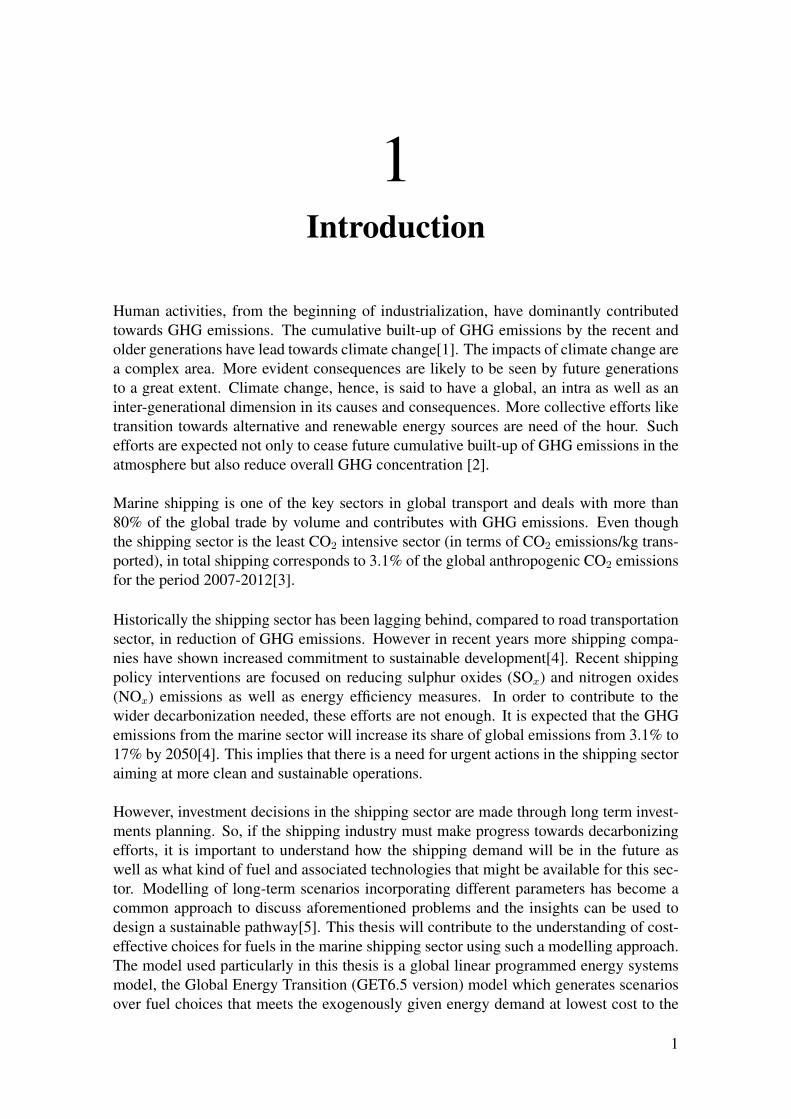
Human activities, from the beginning of industrialization, have dominantly contributedtowards GHG emissions. The cumulative built-up of GHG emissions by the recent andolder generations have lead towards climate change[1]. The impacts of climate change area complex area. More evident consequences are likely to be seen by future generationsto a great extent. Climate change, hence, is said to have a global, an intra as well as aninter-generational dimension in its causes and consequences. More collective efforts liketransition towards alternative and renewable energy sources are need of the hour. Suchefforts are expected not only to cease future cumulative built-up of GHG emissions in theatmosphere but also reduce overall GHG concentration [2].

Marine shipping is one of the key sectors in global transport and deals with more than80% of the global trade by volume and contributes with GHG emissions. Even thoughthe shipping sector is the least CO2 intensive sector (in terms of CO2 emissions/kg trans-ported), in total shipping corresponds to 3.1% of the global anthropogenic CO2 emissionsfor the period 2007-2012[3].

Historically the shipping sector has been lagging behind, compared to road transportationsector, in reduction of GHG emissions. However in recent years more shipping compa-nies have shown increased commitment to sustainable development[4]. Recent shippingpolicy interventions are focused on reducing sulphur oxides (SOx) and nitrogen oxides(NOx) emissions as well as energy efficiency measures. In order to contribute to thewider decarbonization needed, these efforts are not enough. It is expected that the GHGemissions from the marine sector will increase its share of global emissions from 3.1% to17% by 2050[4]. This implies that there is a need for urgent actions in the shipping sectoraiming at more clean and sustainable operations.

However, investment decisions in the shipping sector are made through long term invest-ments planning. So, if the shipping industry must make progress towards decarbonizingefforts, it is important to understand how the shipping demand will be in the future aswell as what kind of fuel and associated technologies that might be available for this sec-tor. Modelling of long-term scenarios incorporating different parameters has become acommon approach to discuss aforementioned problems and the insights can be used todesign a sustainable pathway[5]. This thesis will contribute to the understanding of cost-effective choices for fuels in the marine shipping sector using such a modelling approach.The model used particularly in this thesis is a global linear programmed energy systemsmodel, the Global Energy Transition (GET6.5 version) model which generates scenariosover fuel choices that meets the exogenously given energy demand at lowest cost to the

1

1. Introduction

society. Furthermore, such exercises offer new insights to understand the possible futurerole of alternative fuels.

1.1 Aim and PurposeThe aim of this master’s thesis is to develop demand scenarios for the future shippingsector and evaluate the impact of demand scenarios on the cost-effective fuel choices ina carbon constrained world. Sensitivity analyses will be done based upon scenario ar-guments eg. decarbonisation due to global carbon tax implementation, demand variationthat depend on economic growth.

This master’s thesis will address the following specific research questions:• How may the future shipping demand develop? What change in trade commodities

is expected?• How may different shipping demand scenarios influence the long term and cost-

effective fuel choice in the shipping sector in a carbon constrained world?

The hope is to provide input to policy makers and shipping stakeholders aiming at design-ing pathways for sustainable development in the shipping sector. The purpose is to assessthe role of future alternative and renewable marine fuels and provide support to differentstakeholders in decision making about future renewable marine fuels and its correspond-ing propulsion technology.

1.2 LimitationsThe future shipping demand will depend on many different variables. But not all thefactors will be considered in this study due to the limited amount of time available. Thefocus will be on the factors considered most important. In addition, the GET-RC 6.5model does not considers other GHGs except CO2

1. The thesis does not aim to predictfuture development of global energy system, as this is not the aim of the model tool used.Any future changes in the development of global energy system might affect the resultof marine transport fuels. It is hard to predict upcoming disruptive technologies in thelong-term future. Hence, the results are more limited by the virtue of present knowledgein the marine shipping sector as well as in the entire global energy system.

Apart from limitations in the modelling tool (GET-RC 6.5) applied, emission factors andsize of ship are generalized to calculate the number of ships required using average powerinputs and average annual cargo movements (see section 3.1 for brief information).

1Equivalent CO2 emissions due to methane leakage in case of liquified natural gas combustion has beenconsidered while calculating aggregated CO2 emissions

2

2Scenarios

Demand scenarios in the shipping sector form a part of the global energy system sce-narios. The assumptions made while modelling part of the transport sector or the wholeglobal energy system are supposed to be consistent. For a better understanding of sce-nario approaches, it is important to know how models are generated at a system level ora sector level. Hence, a literature review of different approaches carried out while mod-elling global energy system or a sector of a global energy system, in this case it is theshipping sector, is carried out. In addition, the second half of this chapter provides rele-vant information about different CO2 reduction strategies possible in the shipping sectorand detailed information on Socio-economic Shared Pathway(SSP) approach.

2.1 Previous Global Energy System Scenarios

There is still a limited understanding of the complex interactions between Earth’s cli-mate system and influences due to human activities. From the time the issue of climatechange was realized, significant progress has been done in modelling the future impactsof climate change to reveal future impacts on socio-economic, technological, and envi-ronmental conditions of global society.

There has been significant effort into climate change modelling from 1896 when Arrhe-nius estimated CO2 induced warming of earth’s atmosphere[6]. The IntergovernmentalPanel on Climate Change (IPCC) published the scenarios IS92 in 1992, focusing on en-ergy system development and economic growth scenarios for different regions[7]. Thesescenarios forecasted anthropogenic emissions until year 2100. As many weaknesses werefound in the IS92 modelling exercise there was soon a need for in-depth modelling to geta clearer picture of climate change impacts. The set of SRES scenarios were publishedin year 2000 to overcome the weaknesses found in IS92[8]. These scenarios were recog-nized as four storylines based on 1) Global, 2) Economic, 3) Regional, 4) Environmentalfactors. It was assumed that the future will be shaped by population, economy, technol-ogy, energy, and agricultural (land use) factors. But Moss et al. (2010) argues that all thescenarios so far were fixated towards generating impacts and did not consider the fact thatclimate change impacts will shape socio-economic, technological conditions of the futuresociety as well[9]. This has led towards a novel approach of scenario modelling based oncapability of human society towards climate change mitigation and adaptation.

Socio-economic shared pathways (SSP) are the most recent set of scenarios that describefuture changes in demographics, human development, economy, lifestyle, policies and in-

3

2. Scenarios

stitutions, technology, and environment and resources[10]. These scenarios contain a setof five different scenarios with combination of high or low challenges to mitigation andadaptation, where the fifth is described as moderate challenges to both.

2.1.1 Different Emission Scenario Modelling Approaches for the Ship-ping Sector

For the shipping sector, many researchers have modelled future emission scenarios for theshipping sector until 2050[3, 11, 12, 13, 14, 15].

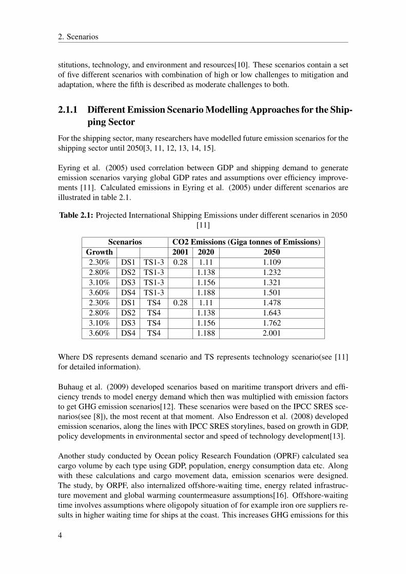
Eyring et al. (2005) used correlation between GDP and shipping demand to generateemission scenarios varying global GDP rates and assumptions over efficiency improve-ments [11]. Calculated emissions in Eyring et al. (2005) under different scenarios areillustrated in table 2.1.

Table 2.1: Projected International Shipping Emissions under different scenarios in 2050[11]

Scenarios CO2 Emissions (Giga tonnes of Emissions)Growth 2001 2020 20502.30% DS1 TS1-3 0.28 1.11 1.1092.80% DS2 TS1-3 1.138 1.2323.10% DS3 TS1-3 1.156 1.3213.60% DS4 TS1-3 1.188 1.5012.30% DS1 TS4 0.28 1.11 1.4782.80% DS2 TS4 1.138 1.6433.10% DS3 TS4 1.156 1.7623.60% DS4 TS4 1.188 2.001

Where DS represents demand scenario and TS represents technology scenario(see [11]for detailed information).

Buhaug et al. (2009) developed scenarios based on maritime transport drivers and effi-ciency trends to model energy demand which then was multiplied with emission factorsto get GHG emission scenarios[12]. These scenarios were based on the IPCC SRES sce-narios(see [8]), the most recent at that moment. Also Endresson et al. (2008) developedemission scenarios, along the lines with IPCC SRES storylines, based on growth in GDP,policy developments in environmental sector and speed of technology development[13].

Another study conducted by Ocean policy Research Foundation (OPRF) calculated seacargo volume by each type using GDP, population, energy consumption data etc. Alongwith these calculations and cargo movement data, emission scenarios were designed.The study, by ORPF, also internalized offshore-waiting time, energy related infrastruc-ture movement and global warming countermeasure assumptions[16]. Offshore-waitingtime involves assumptions where oligopoly situation of for example iron ore suppliers re-sults in higher waiting time for ships at the coast. This increases GHG emissions for this

4

2. Scenarios

specific commodity. Energy related infrastructure demand such as future LNG pipelinesbetween countries are evaluated until 2050 considering construction in progress. Recy-cling assumptions of iron was considered to adjust the calculations. The major argumentOPRF study considers is the global warming countermeasure ability. It is assumed thatthere will be counter actions from the future global society to combat global warmingimpacts. A part of shipping demand is assumed to be satisfied locally in the ORPF model.

Chang et al. (2012) studied the close relationship between marine energy consumption,GDP and GHG emissions. It is found that different parts of the world have differentfeedback relationship in the short-run as well as in the long-run. But there existed somerelationship in between these three factors. The relationship in the regions was eitherunidirectional i.e. A caused B or bidirectional i.e. A causes B and B causes A, a mutualfeedback relationship[17].

Vergara et al. (2012) discussed strategies for reduction in emissions for the passengerand freight maritime sector using projected emissions based on IPCC SRES scenarios.The study discusses the capability of new fuels in the maritime sector to reduce emis-sions. This study estimates that 22% i.e. approximately 370 Million tons of CO2/yearcould be saved using alternative fuels[18]. The pointed-out strategies were not enoughto reach the reduction target, assuming that the maritime sector is held responsible for itsreduction share of the overall emission target. Author asserts that only 62% target waspossible to achieve i.e. 1Gt/yr reduction was possible if all the strategies are adopted atthe same time. This analysis emphasized the need of more international rules and policiesunder IMO to reach such a reduction target.

The latest GHG study performed by IMO (the third) highlights different GHG emissionscenarios based on the mix of SSP+RCP scenarios[15] (for more detailed information onSSP and RCP scenarios see [19]and [20] respectively). This study projects the maritimedemand for cargo types using correlation between GDP and demand. The analysis doneby Ebi et al. (2014) showed no saturation in overall demand as it is strongly coupled toeconomic growth (in terms of GDP). Overall projected emissions in the shipping sectorare presented in the table 2.2.

5

2. Scenarios

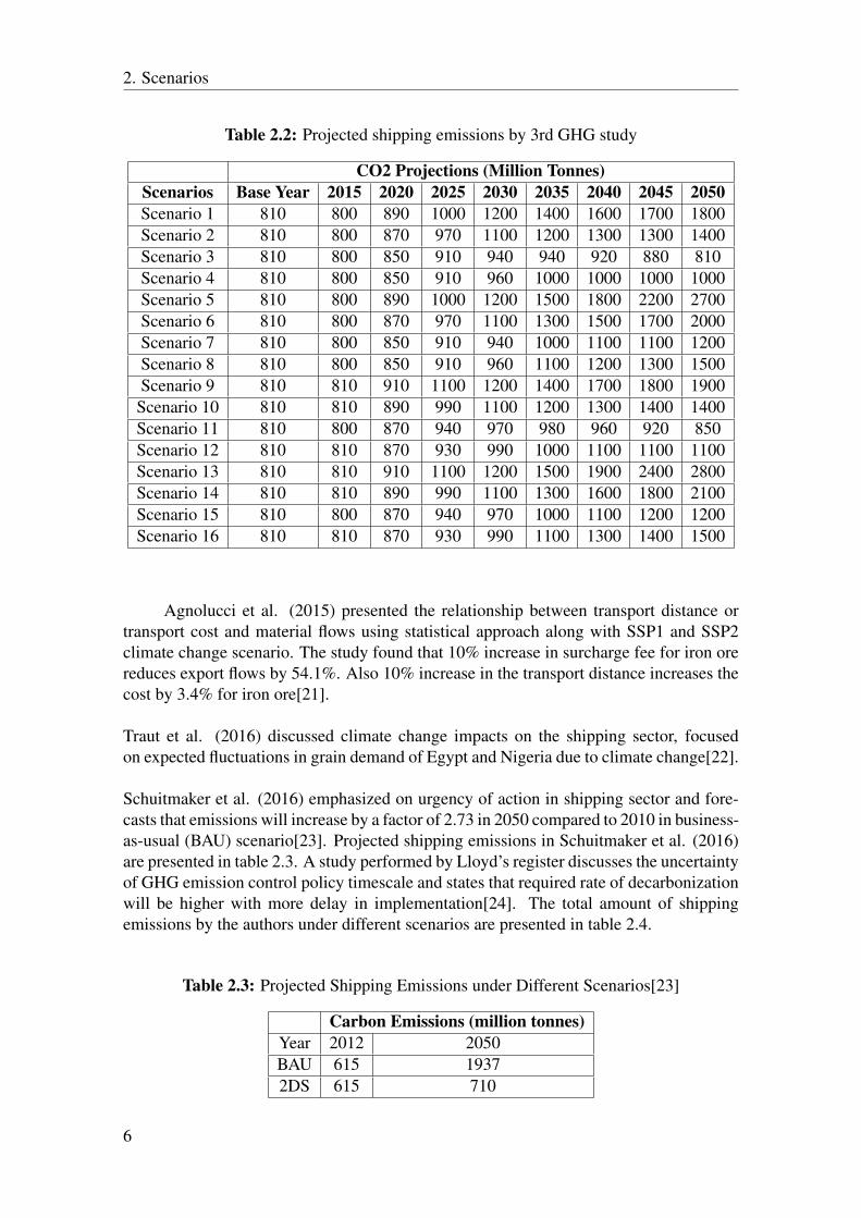
Table 2.2: Projected shipping emissions by 3rd GHG study

CO2 Projections (Million Tonnes)Scenarios Base Year 2015 2020 2025 2030 2035 2040 2045 2050Scenario 1 810 800 890 1000 1200 1400 1600 1700 1800Scenario 2 810 800 870 970 1100 1200 1300 1300 1400Scenario 3 810 800 850 910 940 940 920 880 810Scenario 4 810 800 850 910 960 1000 1000 1000 1000Scenario 5 810 800 890 1000 1200 1500 1800 2200 2700Scenario 6 810 800 870 970 1100 1300 1500 1700 2000Scenario 7 810 800 850 910 940 1000 1100 1100 1200Scenario 8 810 800 850 910 960 1100 1200 1300 1500Scenario 9 810 810 910 1100 1200 1400 1700 1800 1900

Scenario 10 810 810 890 990 1100 1200 1300 1400 1400Scenario 11 810 800 870 940 970 980 960 920 850Scenario 12 810 810 870 930 990 1000 1100 1100 1100Scenario 13 810 810 910 1100 1200 1500 1900 2400 2800Scenario 14 810 810 890 990 1100 1300 1600 1800 2100Scenario 15 810 800 870 940 970 1000 1100 1200 1200Scenario 16 810 810 870 930 990 1100 1300 1400 1500

Agnolucci et al. (2015) presented the relationship between transport distance ortransport cost and material flows using statistical approach along with SSP1 and SSP2climate change scenario. The study found that 10% increase in surcharge fee for iron orereduces export flows by 54.1%. Also 10% increase in the transport distance increases thecost by 3.4% for iron ore[21].

Traut et al. (2016) discussed climate change impacts on the shipping sector, focusedon expected fluctuations in grain demand of Egypt and Nigeria due to climate change[22].

Schuitmaker et al. (2016) emphasized on urgency of action in shipping sector and fore-casts that emissions will increase by a factor of 2.73 in 2050 compared to 2010 in business-as-usual (BAU) scenario[23]. Projected shipping emissions in Schuitmaker et al. (2016)are presented in table 2.3. A study performed by Lloyd’s register discusses the uncertaintyof GHG emission control policy timescale and states that required rate of decarbonizationwill be higher with more delay in implementation[24]. The total amount of shippingemissions by the authors under different scenarios are presented in table 2.4.

Table 2.3: Projected Shipping Emissions under Different Scenarios[23]

Carbon Emissions (million tonnes)Year 2012 2050BAU 615 19372DS 615 710

6

2. Scenarios

Table 2.4: Projected Shipping Emissions in Low Carbon Pathways[24]

Scenario Emissions(Million tonnes)BAU 1400

High Hydrogen 700High Bio mix 600

High Offsetting 1000

Taljegård et al. (2014) asserts that the transition in the use of marine fuels i.e. fromHFO to alternative and renewable fuels will start from 2020 and natural gas based fuelssuch as Liquified natural gas and methanol during the time-period 2020-2050[5].

As seen in the most studies mentioned above, the focus is to either model future emis-sion scenarios with assumption over technologies and/or economic growth. The projectedshipping emissions vary among different scenarios ranges in between 700 to 2800 milliontonnes. There seems a limited discussion on the transition of fuel technology and infras-tructure needed in order for the global shipping industry to reduce its GHG emissions.This, despite that, is important to understand which fuels will be cost-effective optionsfor the marine shipping industry when the expected more stringent carbon constraints areimplemented.

2.2 Shipping Demand

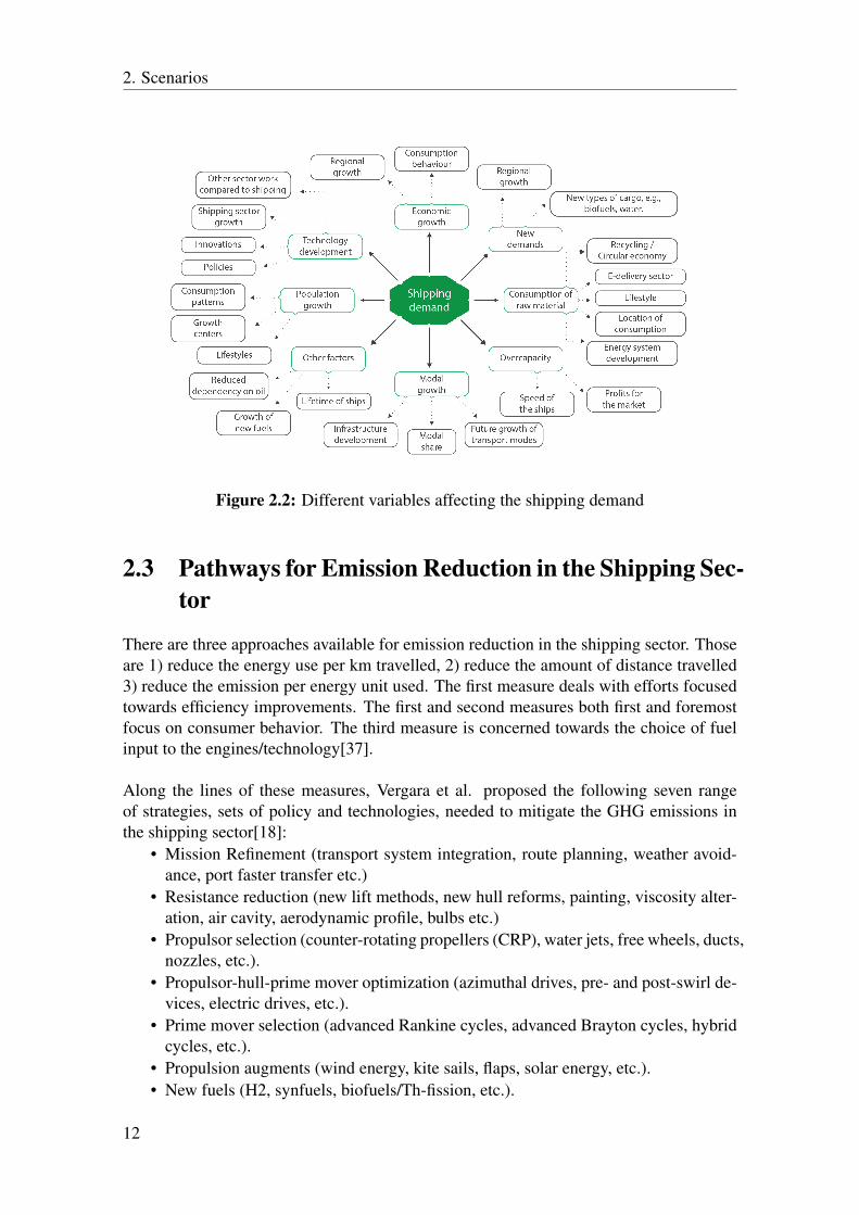
Shipping demand is said to be a derived demand1[25]. It is dependent on the growth inother sectors which increase the need for commodities which are transported by ships.There are a large number of parameters that affect the shipping demand. This sectionbriefly discusses the vital parameters that effect the shipping demand directly. Scientificliterature concludes the principal parameters affecting the shipping demand in present andfuture trends shown in the fig.2.2. Such parameters include:

• Economic Growth• Population• Modal Growth• Technology Development• Consumption of Raw Materials• Overcapacity• New Demands

2.2.1 Economic GrowthEconomic growth results in an increase in personal income. This increases the ability touse more goods and services. So, economic growth can be said to have a direct impacton consumption patterns in the region and in short, can define the need of trade in theregion. The shipping sector satisfies a part of that demand in case some commodities arenot manufactured in the same region or country.

1The demand derived from the demand of another good. In this case, shipping demand changes as thedemand of goods transported through ships changes.

7

2. Scenarios

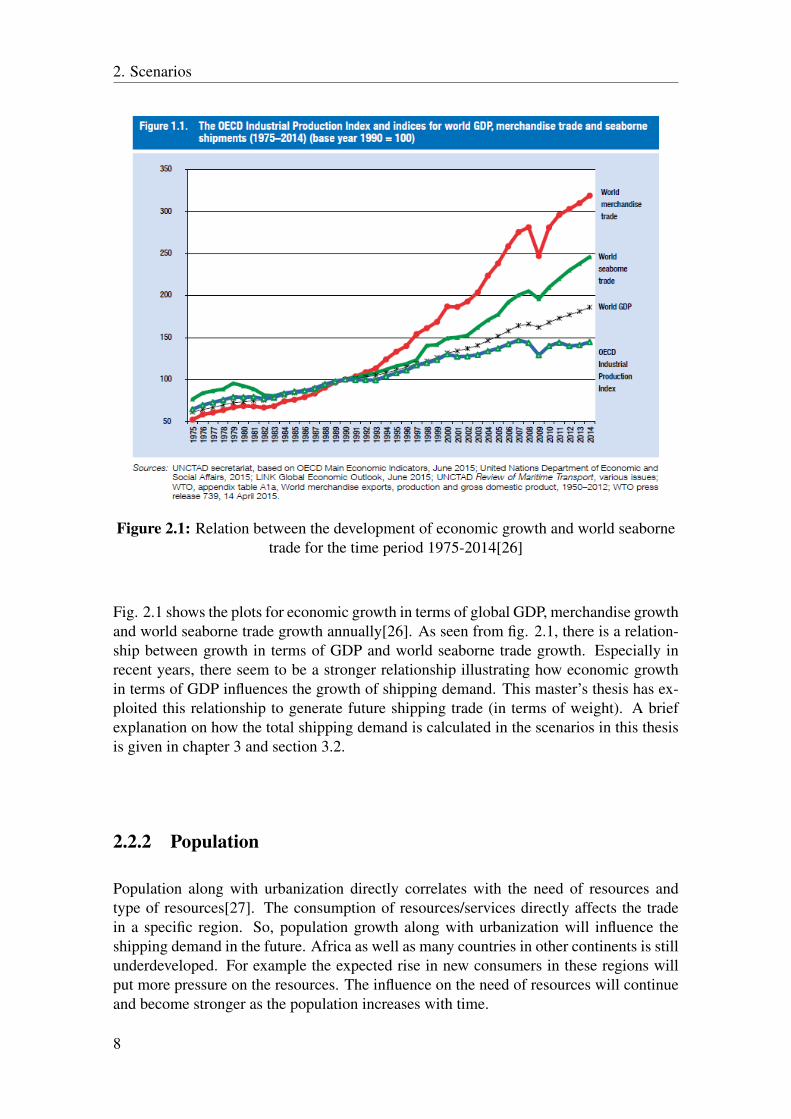
Figure 2.1: Relation between the development of economic growth and world seabornetrade for the time period 1975-2014[26]

Fig. 2.1 shows the plots for economic growth in terms of global GDP, merchandise growthand world seaborne trade growth annually[26]. As seen from fig. 2.1, there is a relation-ship between growth in terms of GDP and world seaborne trade growth. Especially inrecent years, there seem to be a stronger relationship illustrating how economic growthin terms of GDP influences the growth of shipping demand. This master’s thesis has ex-ploited this relationship to generate future shipping trade (in terms of weight). A briefexplanation on how the total shipping demand is calculated in the scenarios in this thesisis given in chapter 3 and section 3.2.

2.2.2 Population

Population along with urbanization directly correlates with the need of resources andtype of resources[27]. The consumption of resources/services directly affects the tradein a specific region. So, population growth along with urbanization will influence theshipping demand in the future. Africa as well as many countries in other continents is stillunderdeveloped. For example the expected rise in new consumers in these regions willput more pressure on the resources. The influence on the need of resources will continueand become stronger as the population increases with time.

8

2. Scenarios

2.2.3 Modal ShareCurrently, all the transport modes are undergoing decarbonization in all possible ways.So, future development of other transport modes will affect the shipping demand, theshipping demand will increase if the other transport modes remain more expensive com-pared to the shipping and if shipping is still a possible choice then the shipping demand isexpected to increase. Policy interventions in different transport sectors can be one of thereason to drive such transformation from one type of transport to another. The shippingdemand is expected to decrease when carbon offsetting cost becomes less expensive forother transport modes compared to marine shipping mode. A reduced demand in this casecould be positive from a climate perspective. In addition, the infrastructure developmentplays a very important role in the advancement of every transport mode. Hence, the devel-opment of other transport modes and the associated future mix of model share will shapethe developments in the shipping sector[28, 29].

2.2.4 Technology DevelopmentTechnology development plays an important role not only in the emission reduction ofthe ship but also affects the growth of alternative fuels. Certain policies are designed topromote the transition to better alternative fuels in parallel with efficiency improvement.Technology development affect the total ship emissions as different fuels/technologieshave different emission factors and need a different infrastructure. These improvementsin technology like efficiency improvements are directly reflected in the capital and oper-ational costs. The costs for reducing emissions will influence the shipping freight rates,and eventually the shipping demand[21]. Not only the technology growth in marine sectormatters but it is important to also understand out-sector growth, e.g. common fuels usedin various sectors. If different sectors are connected via common technology or commonfuel, this might help in reducing the commercial costs.

New innovations might be disruptive. It is difficult to internalize disruptive innovations inenergy systems modelling studies[30].

2.2.5 Raw MaterialsThe commodities, not found/produced locally, involve certain transport mode while trans-porting from one place to another. Such raw materials are most likely transported by seabecause of cheaper freight rates present in the shipping sector. Population and economicgrowth are the major crucial factors that influence the need of such material resources.In addition, there are four important aspects while calculating maritime demand whichare ideal to consider when it comes to the use of the material resources. These are 1)E-delivery sector 2) Location of Consumption 3) Circular Economy 4) Development inEnergy systems[26].

Asia has been a major region where E-delivery sector, the delivery of goods bought overinternet, has boomingly increased in recent years. Digitalization has brought many inter-national markets within the reach of people. Having many developing countries speciallyin Asia region, the E-delivery sector has driven the demand growth in the shipping sector,

9

2. Scenarios

specially in containerships growth[26]. Similar scenarios can happen in Africa countrieswhere the GDP growth is expected to be high in the future.

Location of consumption, hence, is also an important aspect. Most of the countries inthe world are developing now or going to be developing country in the recent future, it isexpected that the capability to buy more products will increase. The demand is expectedto be partly satisfied by the shipping industry since significant amount is shipped to otherparts of the world[26].

The ideas and implementation of the circular economy, which envisions material sym-biosis and maximize the resource utility of any resource[31], are increasing at present.Successful implementation is likely to result in reduced shipping demand directly. Cur-rently there is very little information about the cost required to implement circular econ-omy ideas in various regions.

Also, energy system is transforming towards non-CO2 emitting technologies. The useof CO2 emitting resources, such as oil, coal etc, is expected to decrease, in terms of per-centage, in the future. Trade growth in transporting such resources is very unlikely to takeplace. Use of fossil fuels is expected to decrease and locally produced electricity or fuelsmay be important substitutes, in the transport sector. On the other hand, an increased needof rare earth materials, used in e.g. electric vehicles and wind power industry, may be newcommodities to be traded, leading to an increase of the shipping demand. New resourcesmay or may not need the transportation by the shipping sector.

2.2.6 Overcapacity

The development of larger ships has been seen in the recent years. Theoretically, there isno limit on the size of the ship. But replacement of smaller ships (because of the lifetime)with much larger ships of many fold capacity has taken place[32]. In parallel to increasedoverall capacity, there has been a tiny growth in the marine shipping demand[26] whichhas led to a situation of overcapacity. Overcapacity is destructive towards the shippingmarket as the market may either have lower profits (by lowering freight rates as an effectof that freight rates need to be lowered to get customers to choose the large ships) thanbefore or the shipping market may experience financial loss as the shipping demand islower than available capacity. Overcapacity and lower freight rates were part of the majorreasons for the bankruptcy announced by Hanjin[33], the seventh largest shipping com-pany in the world.

The profits in the shipping market will be defined by the growth in demand. The cur-rent situation with relatively low growth in demand but vast growth in capacity can affectthe growth of the alternative fuels as the companies will focus more on the cheapest fuelrather than alternative fuel to stay in the market. Considering that the fuel consumptionof the ships is proportional to the third power of speed[34], in order to maximize oper-ational profits, the shipping industry have adopted the slow steaming speeds and takingadvantage through better speed management[35].

10

2. Scenarios

A low profit situation, that may arise from overcapacity in the shipping sector, as wellas possible more stringent legislation around emissions are two important challenges forthe shipping industry. Such situations lead to slow transformation into a low-emittingshipping sector[32]. So, depending upon the time overcapacity situation exists in theshipping industry, proportional effects may reflect in delay in actions towards reducingGHG emissions for the shipping sector.

2.2.7 New Demands

At present, the shipping sector transports mainly crude oil, petroleum products, gas, ironore, coal, grain, bauxite, alumina, phosphate rock and containerized sector commodities.With ongoing transformation towards emitting non-CO2 energy system and transport sec-tor, there will be a reduction in the use of oil and coal. Also, climate change is expectedto put more pressure on water availability in many regions. This might affect productionof different commodities in regions. New markets are expected to satisfy an increase indemand in such commodities. A part of such demand can transported through ships, fore.g. expected increase of grains in Egypt[22]. In future, these changes are important toconsider in the model while developing the future demand for shipping. Some insights onthe future mix commodities transported in the marine shipping sector has been discussedin chapter 4 and section (4.1).

Considering the range of impacts from climate change locally as well as globally, a vastrange of variables have started to shape the shipping demand and its cost of operations. Tosummarise, it is forecasted that future shipping demand will be shaped by shifts in globalproduction units, reduced dependence on oil, demographics with changing consumptionpatterns, arrival of bigger container ships, emergence of new sea routes, technology de-velopment, economic growth trends, effect of upcoming circular economy, modal shiftsin other transport sectors, effect of present and future emission control areas (ECAs),prolonged fleet overcapacity and policies interventions[3, 36, 30].

11

2. Scenarios

Figure 2.2: Different variables affecting the shipping demand

2.3 Pathways for Emission Reduction in the Shipping Sec-tor

There are three approaches available for emission reduction in the shipping sector. Thoseare 1) reduce the energy use per km travelled, 2) reduce the amount of distance travelled3) reduce the emission per energy unit used. The first measure deals with efforts focusedtowards efficiency improvements. The first and second measures both first and foremostfocus on consumer behavior. The third measure is concerned towards the choice of fuelinput to the engines/technology[37].

Along the lines of these measures, Vergara et al. proposed the following seven rangeof strategies, sets of policy and technologies, needed to mitigate the GHG emissions inthe shipping sector[18]:

• Mission Refinement (transport system integration, route planning, weather avoid-ance, port faster transfer etc.)

• Resistance reduction (new lift methods, new hull reforms, painting, viscosity alter-ation, air cavity, aerodynamic profile, bulbs etc.)

• Propulsor selection (counter-rotating propellers (CRP), water jets, free wheels, ducts,nozzles, etc.).

• Propulsor-hull-prime mover optimization (azimuthal drives, pre- and post-swirl de-vices, electric drives, etc.).

• Prime mover selection (advanced Rankine cycles, advanced Brayton cycles, hybridcycles, etc.).

• Propulsion augments (wind energy, kite sails, flaps, solar energy, etc.).• New fuels (H2, synfuels, biofuels/Th-fission, etc.).

12

2. Scenarios

These measures provide a basic idea about what kind of improvements exist that arepossible to apply with present state of knowledge[18]. As this thesis is more focuses onthe choice of the fuel, prospective fuels are considered more specifically.

2.3.1 Current Shipping Fuels and Available AlternativesThe current and proposed alternative fuels for the shipping sector is presented in thissection. Current fuels used in the marine sector are Heavy Fuel Oil (HFO) and MarineGas Oil (MGO). The alternative fuels towards the shipping sector include liquified naturalgas (LNG), synthetic fuels, hydrogen, biofuels, e-fuels (fuels produced from electricity,carbon dioxide and water, so called electrofuels) and nuclear fuels. The shipping demandin the military sector is not included in this study. This thesis does not discuss furtheron the nuclear propulsion ships as most of the use of such ships is done in the militarysector[38].

2.3.1.1 Heavy Fuel Oil and Marine Gas Oil

Currently, the shipping fuels are of two types: 1) heavy fuel oils (HFO) and 2) marine gasoils (MGO). HFO is still the most common fuel used in the shipping sector. HFO oil is vis-cous, dirty, and inexpensive. It is similar to the fuel-oil used in the road transport but hasa high viscosity. Viscosity suggests the complexity of fuel heating and handling systemas there is a need for heating to correct injection pressure for optimized performance[39].Approximately, 80% of the fuel used in the shipping industry is HFO and remaining 20%is MGO. A tiny amount of LNG is used in the current shipping sector[40].

HFO consists of approx. 2.7% sulphur on an average. This limit is 2700 times greaterthan the fuel used in road transportation sector[39].

MGO costs in the same range as HFO but has lower sulphur content. The recent pol-icy standards of 0.1% and 0.5% global sulphur concentration limits[41] in certain areashave started this shift towards increased use of MGO. These emission control zones areknown as Sulphur Emission Control Areas (SECA). These SECAs imposed the limit of1% sulphur limit from 1st July 2010 and 0.1% sulphur limit from 2015. In other areas,the sulphur limit has been lowered to 3.5% in 2012. The global limit is expected to go to0.5% effective from 2020 or 2025[41].

2.3.1.2 Liquified Natural Gas

LNG has been a proven and feasible solution for the shipping sector as a fuel. LNGis one of the potential solutions for upcoming regulations limiting CO2, SOx & NOx.It is one of the solutions for SOx reduction but parts of the industry seems to use thescrubber technology with high sulphur content fuel as an alternative way to reduce thesulphur emissions. The price of LNG is relatively low as compared to present fuel. Butthe handling costs are still high. The use of LNG presents some important risks towardsinfrastructure such as explosion hazard in case of leakage, high energy content whenstored under very low temperature. LNG fuel requires more space unless stored at verylow temperature.

13

2. Scenarios

2.3.1.3 Synthetic Fuels

Synthetic fuels are Coal-to-Liquid (CTL), Biomass-to-Liquid (BTL) and Gas-to-Liquid(GTL). These fuels can have the same end-product with different raw material in thebeginning. Synthetic fuels are produced from syngas, a mixture of carbon monoxide andhydrogen, using for example a process called Fischer-Tropsch process. Such type of fuelshas not been used in ships until now. But these fuels can be used in for example heavydiesel engines without any modification. These fuels have lower CO2 and PM emissionsas compared with HFO and MGO with no sulphur emissions. These fuels have lower CO2emissions but not zero. These fuels can be a solution for the marine shipping sector whenmoderate or higher emissions limits are imposed. If the stringent CO2 limits are put forth,most likely these fuels will be a transitional solution until non-CO2 emitting resource andcorresponding technology become commercial. At present, the future looks bleak for theCCS technology to be implemented in the marine shipping sector.

2.3.1.4 Hydrogen

Hydrogen is also another option using a fuel cell or combustion technology. This technol-ogy is not a cost competitive fuel option right now but with improvements in technologyand cost reductions in fuel cell technology, the operations are possible. Hydrogen solvesmany challenges which are perceived towards other intermittent sources. Hydrogen iscommon in nature, but almost always hardly bound in molecule structures meaning thatit demands energy to generate pure H2 and the cost is currently very high. Its lower en-ergy density compared to HFO requires six to seven times more space[42]. Further, thestorage requires well-insulated tanks as it can be flammable under certain conditions. Be-cause of non-CO2 emission when combusted or used in a fuel cell, hydrogen seems asa most promising fuel which can replace fuels in road transportation area. However, theemissions depend on how the hydrogen is produced.

2.3.1.5 Biofuels

A wide range of biofuels are possible to use in present engine technologies with none orsmall modifications. These fuels are often dividied into three types i.e. 1st generation, 2ndgeneration and 3rd generation biofuels. These types vary based on their input source. 1stgeneration biofuels are the fuels that are based on organic material and naturally degradedwhilst the product is taken care of, e.g. ethanol from sugarcane, biogas from digestion etc.Furthermore 2nd generation biofuels have origin from biomass but this biomass is treatedthermally or chemically in order to make products, e.g. ethanol from biomass throughgasification or fermentation. 3rd generation biofuels are viewed as fully synthetic fuelswhich do not depend upon biomass (by-products from biomass process can be used), e.g.electrofuels[43]. From a lifecycle perspective, most biofuels are carbon positive since theproduction lead to GHG emissions. Biofuels do generally have a lower energy content perliter of fuels, compared to HFO, which results in a need for larger storages tanks, onboardthe ship, in order to keep the same fuelling frequency.

14

2. Scenarios

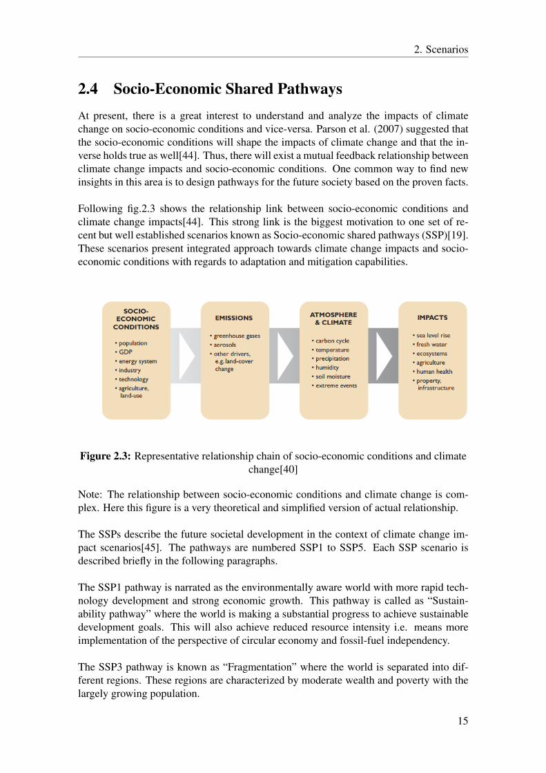
2.4 Socio-Economic Shared PathwaysAt present, there is a great interest to understand and analyze the impacts of climatechange on socio-economic conditions and vice-versa. Parson et al. (2007) suggested thatthe socio-economic conditions will shape the impacts of climate change and that the in-verse holds true as well[44]. Thus, there will exist a mutual feedback relationship betweenclimate change impacts and socio-economic conditions. One common way to find newinsights in this area is to design pathways for the future society based on the proven facts.

Following fig.2.3 shows the relationship link between socio-economic conditions andclimate change impacts[44]. This strong link is the biggest motivation to one set of re-cent but well established scenarios known as Socio-economic shared pathways (SSP)[19].These scenarios present integrated approach towards climate change impacts and socio-economic conditions with regards to adaptation and mitigation capabilities.

Figure 2.3: Representative relationship chain of socio-economic conditions and climatechange[40]

Note: The relationship between socio-economic conditions and climate change is com-plex. Here this figure is a very theoretical and simplified version of actual relationship.

The SSPs describe the future societal development in the context of climate change im-pact scenarios[45]. The pathways are numbered SSP1 to SSP5. Each SSP scenario isdescribed briefly in the following paragraphs.

The SSP1 pathway is narrated as the environmentally aware world with more rapid tech-nology development and strong economic growth. This pathway is called as “Sustain-ability pathway” where the world is making a substantial progress to achieve sustainabledevelopment goals. This will also achieve reduced resource intensity i.e. means moreimplementation of the perspective of circular economy and fossil-fuel independency.

The SSP3 pathway is known as “Fragmentation” where the world is separated into dif-ferent regions. These regions are characterized by moderate wealth and poverty with thelargely growing population.

15

2. Scenarios

The SSP4 pathway corresponds to a world of inequality where developed rich countriesare responsible for GHG emissions and undeveloped countries are more prone towardsclimate change impacts.

The SSP5 pathway is based on conventional development where world development ismaking more progress in terms of economic growth but with the use of energy systemwith high usage of fossil fuels. Economic growth is considered the solution towards botheconomic and social problems faced by individuals. In short, the world will make progresstowards the future following the development seen in developed countries with high useof fossil energy.

Combining all the scenarios together, the SSP2 pathway is designed with the economicand technical development a seen in the scenario in SSP5 and the world is also makingprogress towards achieving sustainability development goals like in SSP3. There will stillbe some inequality in the world where rich countries are still held somewhat responsiblefor the GHG emissions and where poor countries are prone to climate change impactslike in SSP4 but to a lower extent. Some countries will still be poor and will find hard tomaintain living standards of the growing population. The design of SSP2 scenario can besaid as the pathway based on the past trends and slowly lead towards sustainability andefforts will continue to increase as the time passes by. A more detailed version of theSSP scenarios can be found in O’Neill et al. (2014)[10]. The reasons behind choosingSSP2 scenarios for the development of the shipping demand in this study are discussed inchapter 3 and section 3.1.

16

3Methods

This thesis is an example of global energy system modelling exercise where the shippingtransport sector is modelled in detail. The strong relationship of the shipping demand withthe economic growth and population is the base for calculating future shipping demand.The developed shipping demand scenarios is then implemented in the developed versionof the GET model.

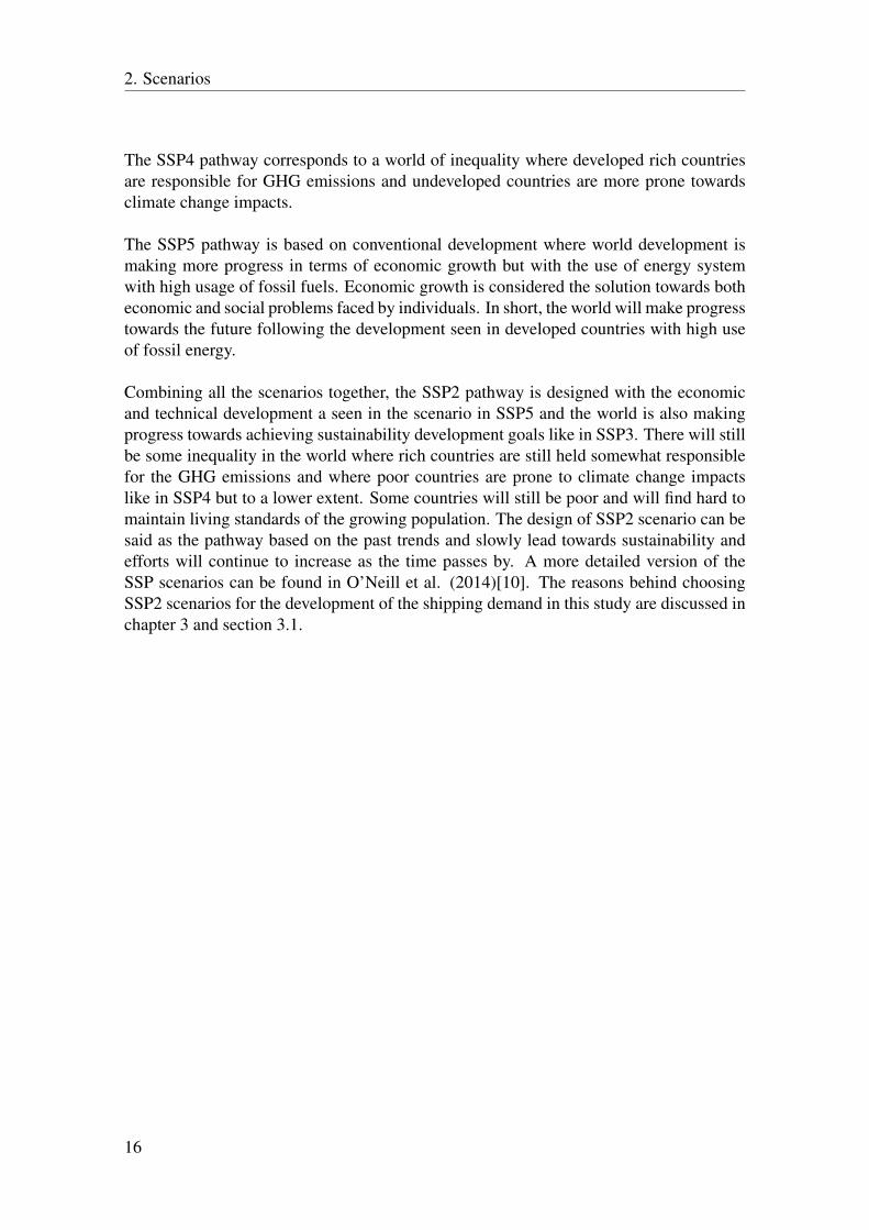
3.1 GET ModelThe Global energy transition model is a cost minimization decision-making tool focusedon satisfying the global energy demand with the available energy supply assuming strin-gent CO2 reduction targets. This model was originally developed in the late 1990s[46]with the aim of analyzing minimum cost solutions given carbon constraint. Since thenthe model has been updated and at present mainly GET-RC 6.5 version is in use[47]. Anoverview of the GET-RC 6.5 model is shown in fig.3.1.

Figure 3.1: The basic flow chart of primary energy supply and fuel choices in the GETModel[40]

The model has 10 different regions with a major focus on the transportation sector. Thislinear optimization model chooses primary energy resources, conversion technologies,energy carriers and transportation technologies which meet the global energy demand at

17

3. Methods

least cost for every region when subjected to carbon constraints. The solutions for eachregion are aggregated to present the final global solution with possible movement of en-ergy resource between regions.

The model time-period is 1990-2140 with a time step of 10 years. The results in thisstudy are discussed for the time-period 2010-2100.

The energy demand in this model is divided into three parts i.e. 1) electricity, 2) heat,and 3) transportation. The electricity sector stands for the electricity demand for everyregion. The heat sector includes all the energy demand that is neither electricity nor trans-port fuels. The transportation sector has been modelled with most details compared toelectricity and heat sector. The transportation sector is divided into two sub-sectors: 1)Passenger demand and 2) Freight demand.

In this thesis the GET-RC model has been developed into model version GET-RC 6.5.Passenger demand in the GET-RC 6.5 model is divided into cars and buses. Also freightsector is divided into trucks, rail, aviation and ships. These demands are function of globalpopulation and economic growth data.

Shipping demand under passenger sector is not considered in this sector since most ofpassenger ships have certain cargo capacity and most likely such ships are taken into con-sideration when shipping demand is expressed in billion ton-miles. In this updated modelversion, GET-RC6.5, the shipping demand under the freight demand is divided into sixdifferent sectors based on commodity types. The commodity types in the shipping sectorinclude:

1. Main bulk materials;2. Gas;3. Oil;4. Chemicals;5. Other bulk materials;6. Containerships.

These categories are modelled using data extracted from the reports mentioned in Reviewof Maritime Transport documents published annually by United Nations Conference onTrade and Development[30, 48, 26, 36]. Each category under the shipping transport sectorrepresents the demand for the respective commodity transported through the ships. TheEuropean Maritime Safety Agency offers the “Equasis” database that comprises informa-tion on the merchant fleet based on the lifetime, average sizes (in deadweight tonnes) andnumber of different types of ships in the shipping sector[49, 50, 51]. This information inaddition to the information about annual cargo capacity and annual transport days by dif-ferent commodity ships[12] is used to total fleet capacity in the marine shipping transportsector.

The information about the technologies used in these six different shipping sectors likecapital cost, lifetime, size of the ships and engine costs is approximated using the avail-able information in previous GET-RC 6.4 model[47].

18

3. Methods

The types of ship in the shipping sector in the earlier GET-RC model versions were basedon vessel and engine size. These types were divided into three categories i.e. coast, oceanand container ships[5] based on the categorization present in Buhaug et. al (2009)[12].

In this thesis the GET-RC model has, further, been developed with an updated generalenergy demand for the heat and electricity sectors following IIASA SSP2-scenario, whereprevious model version has been built on the much older IIASA C1 scenario[52]. All thedemand values are pre-fed into the GET model and these values do not change over thespecific run.

Mature cost data is used for all technologies including the shipping sector. The costsof different technologies are average numbers found through different research articles,reports, and company publications. The propulsion technologies in the shipping sectorconsidered in this model are combustion and fuel cell technology. For more informationabout technology costs and efficiencies of different propulsion technologies, please seeappendix 3. The shipping transport sector includes the marine fuels mentioned in thechapter 2 and section 2.3.1. This includes HFO/MGO, LNG, Biofuels, Synfuels, hydro-gen and electrofuels(fuels produced from CO2 and water using electricity as main sourceof energy).

The CO2 concentration cap limits for each step are extracted from the atmospheric stabi-lization CO2 concentrations presented by Wigley et al.(1996)[53]. It is possible to intro-duce different CO2 concentration levels/caps. Four different CO2 concentration levels i.e.400, 450, 500 and 550ppm has been used in the GET-RC 6.5 model version. The 400 ppmlevel presents the cap where the CO2 concentration is leveled off at 400ppm or below atthe end of the century and will be used in the base case scenario of this study.

Changes in economic growth data and population has also effect on the final demandof road-based transport sector such as bus, rail, cars and trucks etc. These sub-sectorsunder road-based transport sector are consistent in GET-RC 6.5 model.

3.1.1 Overview of Assumptions and Constraints

The assumptions and constraints are linked to the cost of all different types of technolo-gies, efficiency of engines and other conversion efficiencies, total supply potential of pri-mary sources based on reserves and resources, CCS diffusion and the growth of technolo-gies included in the GET Model.

The primary supply potentials for the fossil fuels i.e. oil and natural gas are constrainedto 12000 EJ and 10000 EJ respectively, twice of the proven reserves in 1990. The globalcoal supply is constrained to 260000 EJ[46].

In the transportation sector, in the base case it is assumed that maximum 20% of thetrucks demand fulfilled with PHEVs and another 20% of HEVs. Further in total, maxi-

19

3. Methods

mum of 60% of the bus demand is fulfilled using HEVs and PHEVs.

Carbon capture and storage (CCS) can be a CO2 reducing technology that can eitherbe assumed becoming large scale available or assumed be a technology that will not takeoff due to e.g. lack of public acceptance. In this study it is assumed that CCS will becomea large scale available technology. In the case when CCS technology is possible to usein the model, further assumptions include zero leakage of the stored CO2. That meansleakage of CO2 stored using the CCS technology does not take place. The aggregatedstorage capacity of CO2 over the entire period 2010-2100 is assumed to be 600 GtC. Theexpansion rate is constrained by maximum 100MtC per decade.

The amount of electricity produced by the nuclear energy is assumed to be constant overthe century. It is assumed that nuclear energy cannot excced the level of today. There isno limitation on the total expansion of the wind and the solar energy but their expansionrate is constrained.

Grahn et al. (2009) assert that the cost-effective use of biomass resources will be inelectricity and heat sector rather than in transportation sector. The limited amount ofbiomass resources available to fulfill the demand and the higher conversion efficiencyin the other sectors is the main reason behind this conclusion[54]. Hedenus et al. (2010)found that maximum 50% of the energy demand in the heat sector will come from biomassresource[55].

3.1.2 Limitations

It is important to understand that the GET-RC 6.5 model is not developed to predict futuredevelopment of the global energy system. It is meant to understand the role of differenttechnologies available in different sectors, inter- and intra-sector interactions, and overallsystem behavior. In addition, it is hard to predict upcoming disruptive technologies in thelong-term future. Hence, the results are more limited by the virtue of present knowledgein the marine shipping sector.

It is possible that the roll-out of different technologies might differ between areas andmaybe different time-period as the time to diffuse in the niche markets vary for differenttechnologies to become commercial. Such differential effects are not seen in the modelresults.

The cost and price elasticity is not present in the GET-RC 6.5 model. Instead, matureand present observed costs are used in the model. Also, the demand scenarios are exoge-nously given for all the ten regions present in the model and the given energy demand donot change when the model is running.

The electricity sectors of each region are not connected to each other. Thus there is nopossibility to transfer electricity between regions. This model does not consider any otherGHG emissions than CO2 emissions, except methane leakage due to combustion of LNGusing combustion engines.

20

3. Methods

The results obtained show a certain possible pathway to achieve the most cost-effectivesolution. This does not mean that the same path will be followed by the fuels at anypoint in time. The results give insight when the technology should be in place in order toreduce the emissions in order to get cost-effective solution for society, the reality mightbe different. Total energy demand calculations for the electricity, the heat as well as thetransportation sector are never exact but the calculations are based on the lifetime of tech-nology, energy efficiency, costs, and resource availability.

While calculating the number of ships, the average size of the engines, average speedand average number of days are taken into consideration. So, uncertainties exist overfinal emissions over the shipping transport sector as well as other sectors.

3.2 Scenarios for the Future Shipping Demand

As mentioned before in section 2.2, the shipping demand scenarios are dependent on sev-eral factors. This thesis focuses mostly on the impact of economic growth and populationas these factors are a representation of global socio-economic conditions which are as-sumed to be drivers of climate change.

The statistics over economic growth and population is collected from Knoema statistics(see www.knoema.com) and World bank (see www.worldbank.org) respectively.

This thesis uses the technique of multivariable regression method to forecast future ship-ping demand. Multivariable regression is a technique to forecast the dependent variablebased on two or more independent variables. This technique is used to learn more aboutthe relationship between dependent and independent variables. Such relationships predictfuture values of dependent variables. In general, suppose, demand d is function of thevariables x1 and x2, then the relationship between demand and the variable is shown as,

d = β0 + β1 ∗ x1 + β2 ∗ x2 (3.1)

Where, x1 is in US$2005 and x2 is the population number. Beta represents the regressioncoefficient connected to the dependent variable.Here, β1 is the regression coefficient for the economic growth and β2 is regression coeffi-cient for the population. For every increase of 1 unit in either of the variables, the positiveregression coefficient represent increase in the demand and vice-versa. R-squared denotesthe measure of how close the data is fitted to the regression line. Using the R-squared val-ues, the correlation coefficient varies between 0 and 1. The relationship is more strong asthe coefficient gets closer to 1.

Here, the independent variables are economic growth and population1 and the depen-dent variable is the trade expressed in billions of ton-miles. The regression analysis is

1It can be said economic growth and population are not exactly independent factors. The main motiva-tion behind considering this assumption is that population has equally important as economic growth whenthe pressure of limited supply sources is considered

21

3. Methods

performed to generate relationship of each demand category under the shipping sector(expressed in terms of billion ton-miles) with economic growth and population. Thisperformed regression analysis presents relationship for every individual commodity typeunder shipping sector (for commodity types,see section 3.1 on page 18).

This thesis has formulated the mathematical relationship to calculate marine shippingdemand as a function of economic growth and population. To model the assumptionsfor the economic growth and population in the context of climate change until 2100, thisthesis incorporates the SSP 2 scenario as a base case to proceed with[45].

This thesis uses the above built relationships between global shipping trade, economicgrowth and population using multivariable regression analysis. This relationship is basedon past data over 25 years. To use this relationship, the demand scenario should considerpopulation and economic growth trends which will follow a similar path as in the past.That means the future trends will follow the recent observed past trends for all the cate-gories. As mentioned in the description of the SSP2 scenario, in section 2.4, the world willfollow a path in which social, economic, and technological trends follow recent historicalpatterns. Therefore, the SSP2 scenario is chosen to be used for the base case scenarioin this thesis and is incorporated in the GET model. Also, other transportation demandcalculations for passenger transport and freight transport except marine shipping sectorare strongly based on the economic growth and population values. This is one anothermotivation to use SSP2 scenario as a base case scenario.

Thus the population and economic growth numbers are updated based on the SSP2 sce-nario. The SSP2 scenario is considered a scenario which offers insights about the socio-economic conditions of future global society[].

3.2.1 Sensitivity Analysis

Besides the base case scenario two additional scenarios are developed and used for sensi-tivity analyses. The reason is that population and economic growth have mutual feedbackrelationship which could be explored more and which makes the population and economicgrowth used in the base case scenario uncertain. In the longer term, population growthmay affect the living standards of the society[56]. There is fixed quantity of resourcespresent in nature and more growth will put pressure at least on those resources whoseproduction cannot be multiplied using present or upcoming technological advances. Also,the uncertain nature of population can have an impact on economic growth and vice-versa.This bi-directional relationship between population and economic growth is not possibleto explore due to limited time in this thesis. It is decided to focus more on economicgrowth and keep the population data constant.

Research carried out under different socio-economic conditions show a range of possibleeconomic growth situations under different conditions - the expected range of economicgrowth varies from 0.8% annual growth in GDP to 2.8% annual[57, 58, 59]. The eco-nomic growth assumed under base case scenario used in this study is approx. 1.6%/year,which represents the economic growth in the SSP2 scenario. The first variant of the base

22

3. Methods

case used for sensitivity analyses is assumed to have almost double rate of economicgrowth in terms of GDPppp i.e. 3.2%/year. The other situation corresponds to approxi-mately half of the growth rate assumed in the base case i.e. 0.8%/year.

There are some concern regarding the feasibility of hydrogen being a marine fuel. Thesensitivity of this nature is addressed in next sensitivity analysis(see section 4.6.2 in chap-ter 4).

In addition, another sensitivity analysis is performed to explore the impact of CO2 taxlevels on the pre-requisites for alternative marine fuels.

23

3. Methods

24

4Results and Analysis

4.1 Trends in Shipping Demand Sector

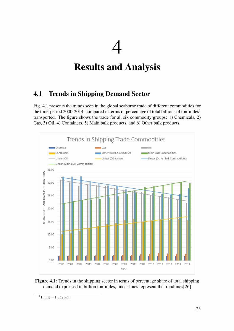
Fig. 4.1 presents the trends seen in the global seaborne trade of different commodities forthe time-period 2000-2014, compared in terms of percentage of total billions of ton-miles1

transported. The figure shows the trade for all six commodity groups: 1) Chemicals, 2)Gas, 3) Oil, 4) Containers, 5) Main bulk products, and 6) Other bulk products.

Figure 4.1: Trends in the shipping sector in terms of percentage share of total shippingdemand expressed in billion ton-miles, linear lines represent the trendlines[26]

11 mile = 1.852 km

25

4. Results and Analysis

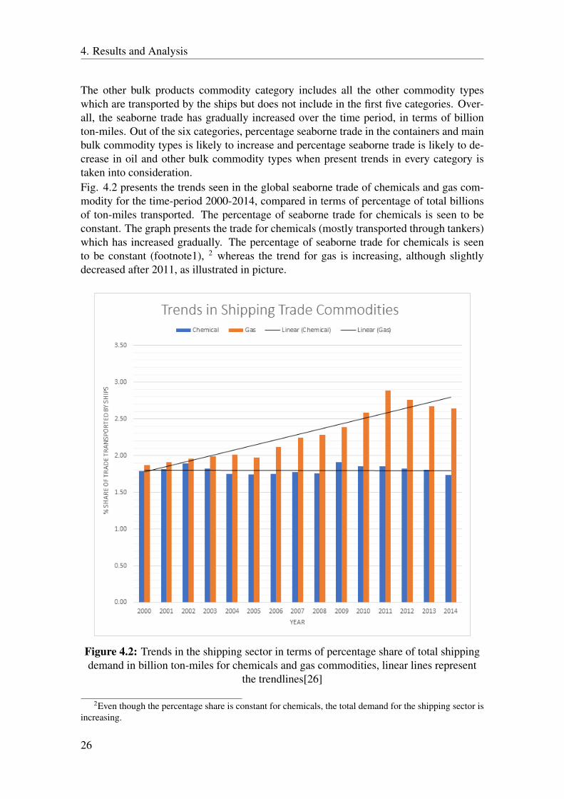
The other bulk products commodity category includes all the other commodity typeswhich are transported by the ships but does not include in the first five categories. Over-all, the seaborne trade has gradually increased over the time period, in terms of billionton-miles. Out of the six categories, percentage seaborne trade in the containers and mainbulk commodity types is likely to increase and percentage seaborne trade is likely to de-crease in oil and other bulk commodity types when present trends in every category istaken into consideration.Fig. 4.2 presents the trends seen in the global seaborne trade of chemicals and gas com-modity for the time-period 2000-2014, compared in terms of percentage of total billionsof ton-miles transported. The percentage of seaborne trade for chemicals is seen to beconstant. The graph presents the trade for chemicals (mostly transported through tankers)which has increased gradually. The percentage of seaborne trade for chemicals is seento be constant (footnote1), 2 whereas the trend for gas is increasing, although slightlydecreased after 2011, as illustrated in picture.

Figure 4.2: Trends in the shipping sector in terms of percentage share of total shippingdemand in billion ton-miles for chemicals and gas commodities, linear lines represent

the trendlines[26]

2Even though the percentage share is constant for chemicals, the total demand for the shipping sector isincreasing.

26

4. Results and Analysis

However, the opposite trends are seen for oil and other-bulk products commodity groups.As mentioned already, since there is ongoing transformation towards non-CO2 emittingresources and technology, the dependency on the use of oil will certainly decrease, imply-ing a potential reduction in trade of this commodity. There is an upward trend for the mainbulk products. This implies that there is likely increase in the use of main bulk productsglobally i.e. iron ore, grains, coal, bauxite, alumina, and phosphate rock. It is expectedthat future trade will be affected by climate change, for example from that the crop yieldmay be changed in the different world regions.[60].

With these trends seen in the recent years, more investments may be seen in the shipswhich can transport containerized products, main bulk products and gas volumes than inships transporting oil products and chemicals. Depending on the possibility to use differ-ent fuels for ships for different commodities this might impact the prerequisites for differ-ent alternative marine fuels. As the economic growth is expected to continue in south-eastAsia and upcoming growth in Africa[57, 58, 59], the overall demand in seaborne trade islikely to increase where as the demand in other regions will saturate as the growth satu-rates in future.

4.2 Estimated Future Shipping Demand

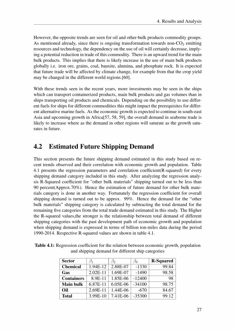
This section presents the future shipping demand estimated in this study based on re-cent trends observed and their correlation with economic growth and population. Table4.1 presents the regression parameters and correlation coefficient(R-squared) for everyshipping demand category included in this study. After analyzing the regression analy-sis R-Squared coefficient for "other bulk materials" shipping turned out to be less than90 percent(Approx.70%). Hence the estimation of future demand for other bulk mate-rials category is done in another way. Fortunately the regression coefficient for overallshipping demand is turned out to be approx. 99%. Hence the demand for the “otherbulk materials” shipping category is calculated by subtracting the total demand for theremaining five categories from the total trade demand estimated in this study. The Higherthe R-squared values,the stronger is the relationship between total demand of differentshipping categories with the past development path of economic growth and populationwhen shipping demand is expressed in terms of billion ton-miles data during the period1990-2014. Respective R-squared values are shown in table 4.1.

Table 4.1: Regression coefficient for the relation between economic growth, populationand shipping demand for different ship categories

Sector β1 β2 β0 R-SquaredChemical 1.94E-12 2.88E-07 -1330 99.84Gas 2.02E-11 1.69E-07 -1490 98.58Containers 8.9E-11 1.85E-06 -12400 98Main bulk 6.87E-11 6.05E-06 -34100 98.75Oil 2.69E-11 1.44E-06 -670 84.67Total 3.99E-10 7.41E-06 -35300 99.12

27

4. Results and Analysis

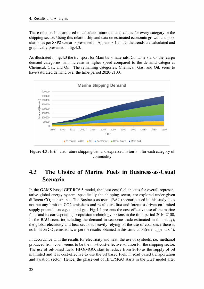
These relationships are used to calculate future demand values for every category in theshipping sector. Using this relationship and data on estimated economic growth and pop-ulation as per SSP2 scenario presented in Appendix 1 and 2, the trends are calculated andgraphically presented in fig.4.3.

As illustrated in fig.4.3 the transport for Main bulk materials, Containers and other cargodemand categories will increase in higher speed compared to the demand categoriesChemical, Gas, and Oil. The remaining categories, Chemical, Gas, and Oil, seem tohave saturated demand over the time-period 2020-2100.

Figure 4.3: Estimated future shipping demand expressed in ton-km for each category ofcommodity

4.3 The Choice of Marine Fuels in Business-as-UsualScenario

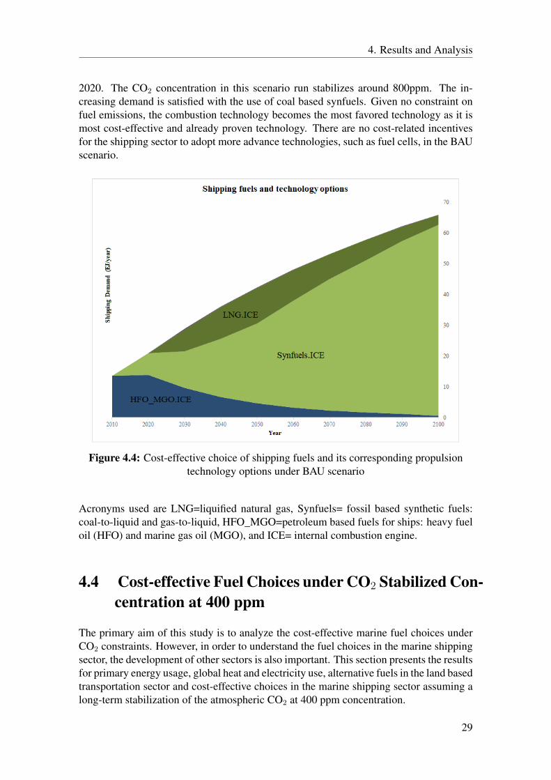
In the GAMS-based GET-RC6.5 model, the least cost fuel choices for overall represen-tative global energy system, specifically the shipping sector, are explored under givendifferent CO2 constraints. The Business-as-usual (BAU) scenario used in this study doesnot put any limit on CO2 emissions and results are first and foremost driven on limitedsupply potential on e.g. oil and gas. Fig.4.4 presents the cost-effective use of the marinefuels and its corresponding propulsion technology options in the time-period 2010-2100.In the BAU scenario(including the demand in seaborne trade estimated in this study),the global electricity and heat sector is heavily relying on the use of coal since there isno limit on CO2 emissions, as per the results obtained in this simulation(refer appendix 4).

In accordance with the results for electricity and heat, the use of synfuels, i.e. methanolproduced from coal, seems to be the most cost-effective solution for the shipping sector.The use of oil-based fuels, HFO/MGO, start to reduce from 2010 as the supply of oilis limited and it is cost-effective to use the oil based fuels in road based transportationand aviation sector. Hence, the phase-out of HFO/MGO starts in the GET model after

28

4. Results and Analysis

2020. The CO2 concentration in this scenario run stabilizes around 800ppm. The in-creasing demand is satisfied with the use of coal based synfuels. Given no constraint onfuel emissions, the combustion technology becomes the most favored technology as it ismost cost-effective and already proven technology. There are no cost-related incentivesfor the shipping sector to adopt more advance technologies, such as fuel cells, in the BAUscenario.

Figure 4.4: Cost-effective choice of shipping fuels and its corresponding propulsiontechnology options under BAU scenario

Acronyms used are LNG=liquified natural gas, Synfuels= fossil based synthetic fuels:coal-to-liquid and gas-to-liquid, HFO_MGO=petroleum based fuels for ships: heavy fueloil (HFO) and marine gas oil (MGO), and ICE= internal combustion engine.

4.4 Cost-effective Fuel Choices under CO2 Stabilized Con-centration at 400 ppm

The primary aim of this study is to analyze the cost-effective marine fuel choices underCO2 constraints. However, in order to understand the fuel choices in the marine shippingsector, the development of other sectors is also important. This section presents the resultsfor primary energy usage, global heat and electricity use, alternative fuels in the land basedtransportation sector and cost-effective choices in the marine shipping sector assuming along-term stabilization of the atmospheric CO2 at 400 ppm concentration.

29

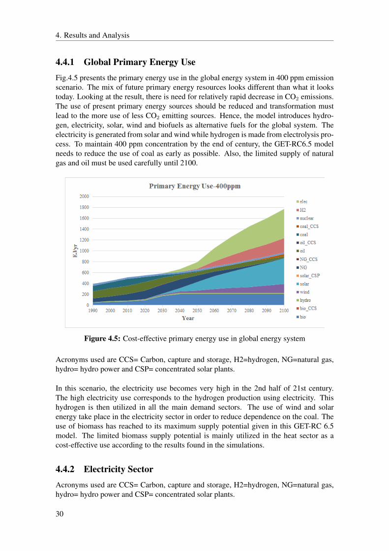
4. Results and Analysis

4.4.1 Global Primary Energy UseFig.4.5 presents the primary energy use in the global energy system in 400 ppm emissionscenario. The mix of future primary energy resources looks different than what it lookstoday. Looking at the result, there is need for relatively rapid decrease in CO2 emissions.The use of present primary energy sources should be reduced and transformation mustlead to the more use of less CO2 emitting sources. Hence, the model introduces hydro-gen, electricity, solar, wind and biofuels as alternative fuels for the global system. Theelectricity is generated from solar and wind while hydrogen is made from electrolysis pro-cess. To maintain 400 ppm concentration by the end of century, the GET-RC6.5 modelneeds to reduce the use of coal as early as possible. Also, the limited supply of naturalgas and oil must be used carefully until 2100.

Figure 4.5: Cost-effective primary energy use in global energy system

Acronyms used are CCS= Carbon, capture and storage, H2=hydrogen, NG=natural gas,hydro= hydro power and CSP= concentrated solar plants.

In this scenario, the electricity use becomes very high in the 2nd half of 21st century.The high electricity use corresponds to the hydrogen production using electricity. Thishydrogen is then utilized in all the main demand sectors. The use of wind and solarenergy take place in the electricity sector in order to reduce dependence on the coal. Theuse of biomass has reached to its maximum supply potential given in this GET-RC 6.5model. The limited biomass supply potential is mainly utilized in the heat sector as acost-effective use according to the results found in the simulations.

4.4.2 Electricity SectorAcronyms used are CCS= Carbon, capture and storage, H2=hydrogen, NG=natural gas,hydro= hydro power and CSP= concentrated solar plants.

30

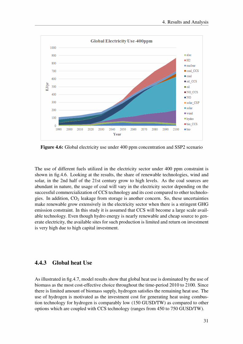
4. Results and Analysis

Figure 4.6: Global electricity use under 400 ppm concentration and SSP2 scenario

The use of different fuels utilized in the electricity sector under 400 ppm constraint isshown in fig.4.6. Looking at the results, the share of renewable technologies, wind andsolar, in the 2nd half of the 21st century grow to high levels. As the coal sources areabundant in nature, the usage of coal will vary in the electricity sector depending on thesuccessful commercialization of CCS technology and its cost compared to other technolo-gies. In addition, CO2 leakage from storage is another concern. So, these uncertaintiesmake renewable grow extensively in the electricity sector when there is a stringent GHGemission constraint. In this study it is assumed that CCS will become a large scale avail-able technology. Even though hydro energy is nearly renewable and cheap source to gen-erate electricity, the available sites for such production is limited and return on investmentis very high due to high capital investment.

4.4.3 Global heat Use

As illustrated in fig.4.7, model results show that global heat use is dominated by the use ofbiomass as the most cost-effective choice throughout the time-period 2010 to 2100. Sincethere is limited amount of biomass supply, hydrogen satisfies the remaining heat use. Theuse of hydrogen is motivated as the investment cost for generating heat using combus-tion technology for hydrogen is comparably low (150 GUSD/TW) as compared to otheroptions which are coupled with CCS technology (ranges from 450 to 750 GUSD/TW).

31

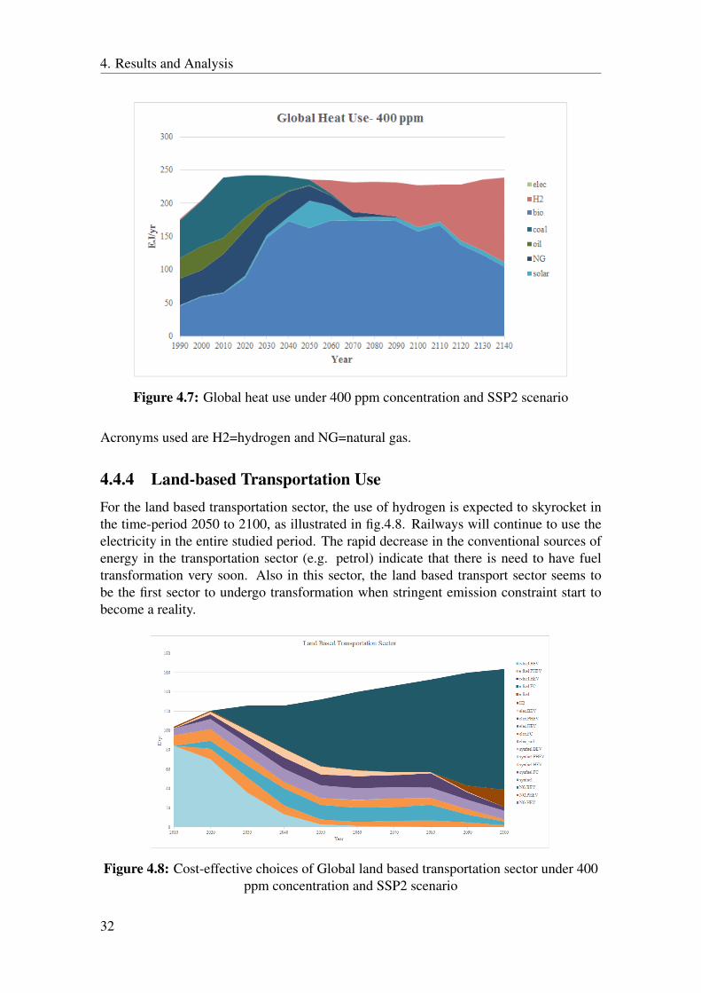
4. Results and Analysis

Figure 4.7: Global heat use under 400 ppm concentration and SSP2 scenario

Acronyms used are H2=hydrogen and NG=natural gas.

4.4.4 Land-based Transportation UseFor the land based transportation sector, the use of hydrogen is expected to skyrocket inthe time-period 2050 to 2100, as illustrated in fig.4.8. Railways will continue to use theelectricity in the entire studied period. The rapid decrease in the conventional sources ofenergy in the transportation sector (e.g. petrol) indicate that there is need to have fueltransformation very soon. Also in this sector, the land based transport sector seems tobe the first sector to undergo transformation when stringent emission constraint start tobecome a reality.

Figure 4.8: Cost-effective choices of Global land based transportation sector under 400ppm concentration and SSP2 scenario

32

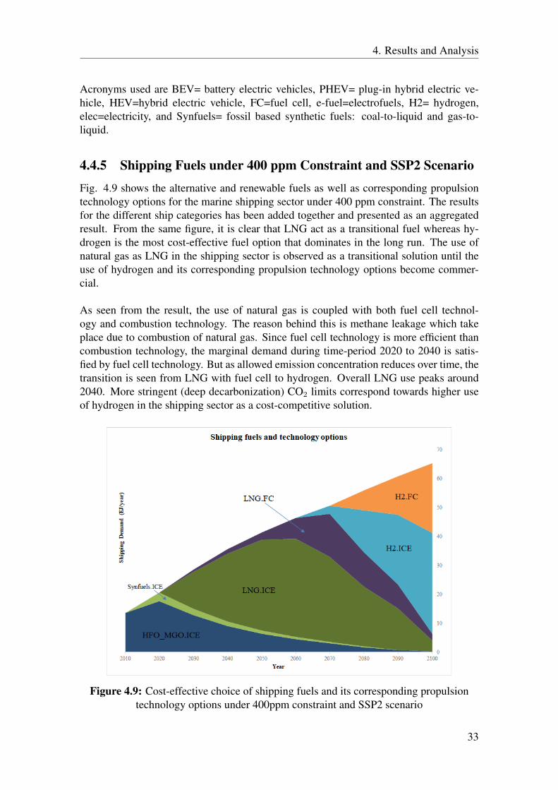
4. Results and Analysis

Acronyms used are BEV= battery electric vehicles, PHEV= plug-in hybrid electric ve-hicle, HEV=hybrid electric vehicle, FC=fuel cell, e-fuel=electrofuels, H2= hydrogen,elec=electricity, and Synfuels= fossil based synthetic fuels: coal-to-liquid and gas-to-liquid.

4.4.5 Shipping Fuels under 400 ppm Constraint and SSP2 Scenario

Fig. 4.9 shows the alternative and renewable fuels as well as corresponding propulsiontechnology options for the marine shipping sector under 400 ppm constraint. The resultsfor the different ship categories has been added together and presented as an aggregatedresult. From the same figure, it is clear that LNG act as a transitional fuel whereas hy-drogen is the most cost-effective fuel option that dominates in the long run. The use ofnatural gas as LNG in the shipping sector is observed as a transitional solution until theuse of hydrogen and its corresponding propulsion technology options become commer-cial.

As seen from the result, the use of natural gas is coupled with both fuel cell technol-ogy and combustion technology. The reason behind this is methane leakage which takeplace due to combustion of natural gas. Since fuel cell technology is more efficient thancombustion technology, the marginal demand during time-period 2020 to 2040 is satis-fied by fuel cell technology. But as allowed emission concentration reduces over time, thetransition is seen from LNG with fuel cell to hydrogen. Overall LNG use peaks around2040. More stringent (deep decarbonization) CO2 limits correspond towards higher useof hydrogen in the shipping sector as a cost-competitive solution.

Figure 4.9: Cost-effective choice of shipping fuels and its corresponding propulsiontechnology options under 400ppm constraint and SSP2 scenario

33

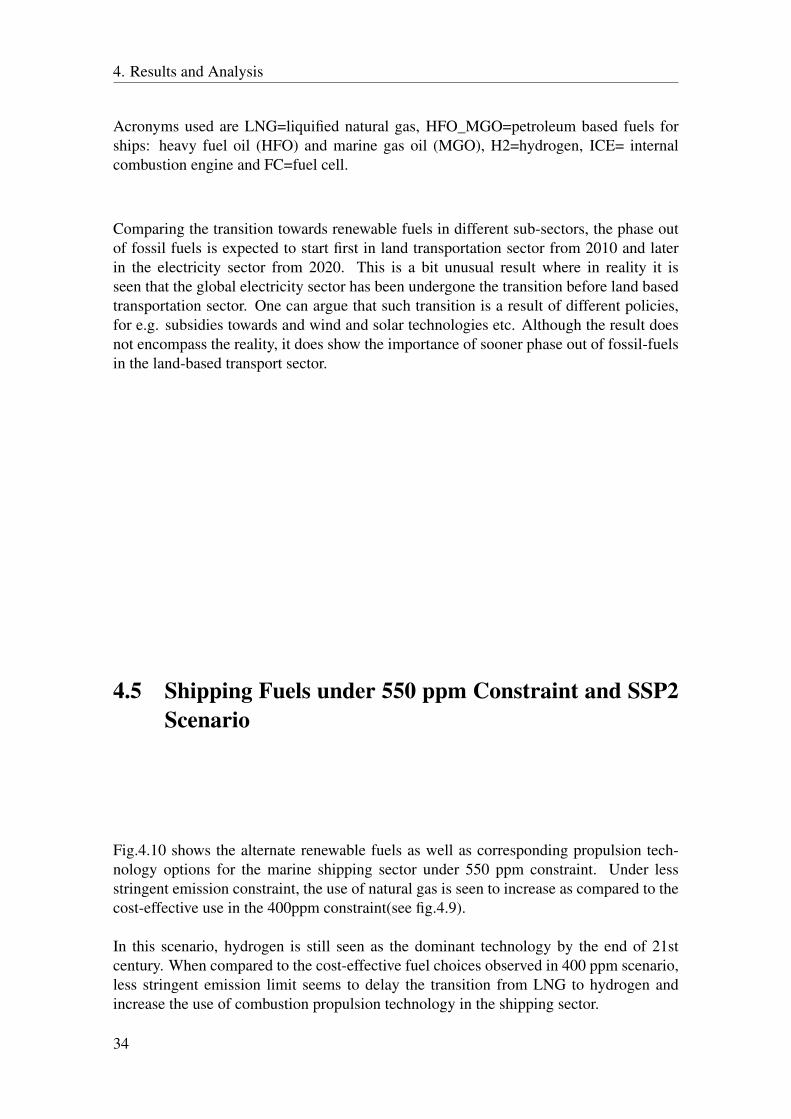
4. Results and Analysis

Acronyms used are LNG=liquified natural gas, HFO_MGO=petroleum based fuels forships: heavy fuel oil (HFO) and marine gas oil (MGO), H2=hydrogen, ICE= internalcombustion engine and FC=fuel cell.

Comparing the transition towards renewable fuels in different sub-sectors, the phase outof fossil fuels is expected to start first in land transportation sector from 2010 and laterin the electricity sector from 2020. This is a bit unusual result where in reality it isseen that the global electricity sector has been undergone the transition before land basedtransportation sector. One can argue that such transition is a result of different policies,for e.g. subsidies towards and wind and solar technologies etc. Although the result doesnot encompass the reality, it does show the importance of sooner phase out of fossil-fuelsin the land-based transport sector.

4.5 Shipping Fuels under 550 ppm Constraint and SSP2Scenario

Fig.4.10 shows the alternate renewable fuels as well as corresponding propulsion tech-nology options for the marine shipping sector under 550 ppm constraint. Under lessstringent emission constraint, the use of natural gas is seen to increase as compared to thecost-effective use in the 400ppm constraint(see fig.4.9).

In this scenario, hydrogen is still seen as the dominant technology by the end of 21stcentury. When compared to the cost-effective fuel choices observed in 400 ppm scenario,less stringent emission limit seems to delay the transition from LNG to hydrogen andincrease the use of combustion propulsion technology in the shipping sector.

34

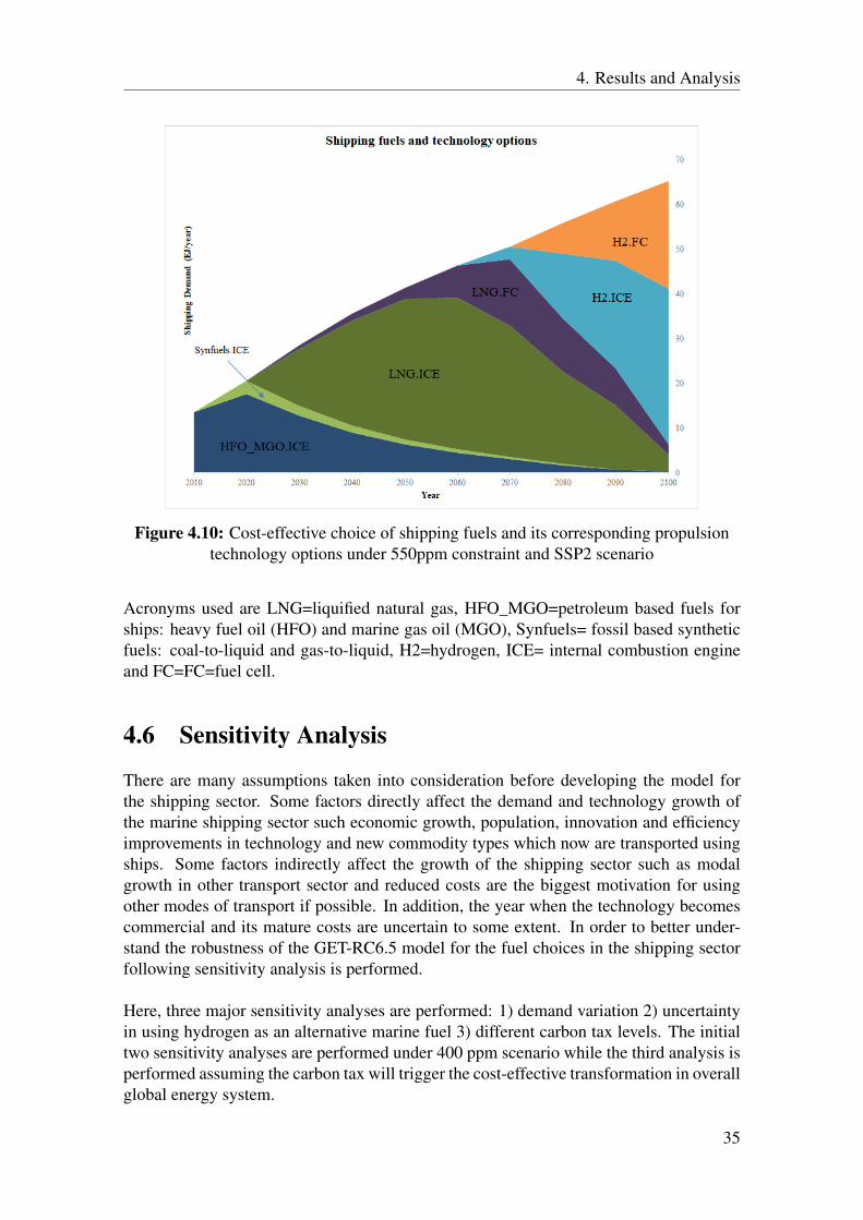
4. Results and Analysis

Figure 4.10: Cost-effective choice of shipping fuels and its corresponding propulsiontechnology options under 550ppm constraint and SSP2 scenario

Acronyms used are LNG=liquified natural gas, HFO_MGO=petroleum based fuels forships: heavy fuel oil (HFO) and marine gas oil (MGO), Synfuels= fossil based syntheticfuels: coal-to-liquid and gas-to-liquid, H2=hydrogen, ICE= internal combustion engineand FC=FC=fuel cell.

4.6 Sensitivity Analysis

There are many assumptions taken into consideration before developing the model forthe shipping sector. Some factors directly affect the demand and technology growth ofthe marine shipping sector such economic growth, population, innovation and efficiencyimprovements in technology and new commodity types which now are transported usingships. Some factors indirectly affect the growth of the shipping sector such as modalgrowth in other transport sector and reduced costs are the biggest motivation for usingother modes of transport if possible. In addition, the year when the technology becomescommercial and its mature costs are uncertain to some extent. In order to better under-stand the robustness of the GET-RC6.5 model for the fuel choices in the shipping sectorfollowing sensitivity analysis is performed.

Here, three major sensitivity analyses are performed: 1) demand variation 2) uncertaintyin using hydrogen as an alternative marine fuel 3) different carbon tax levels. The initialtwo sensitivity analyses are performed under 400 ppm scenario while the third analysis isperformed assuming the carbon tax will trigger the cost-effective transformation in overallglobal energy system.

35

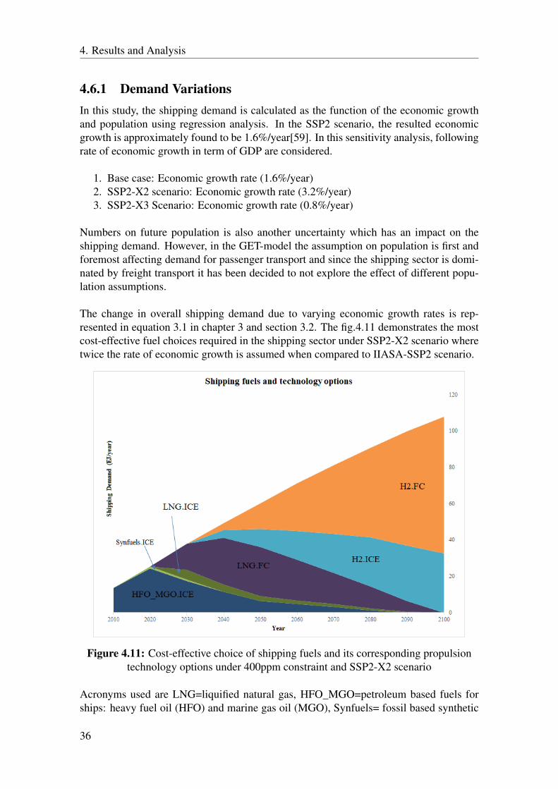
4. Results and Analysis

4.6.1 Demand VariationsIn this study, the shipping demand is calculated as the function of the economic growthand population using regression analysis. In the SSP2 scenario, the resulted economicgrowth is approximately found to be 1.6%/year[59]. In this sensitivity analysis, followingrate of economic growth in term of GDP are considered.

1. Base case: Economic growth rate (1.6%/year)2. SSP2-X2 scenario: Economic growth rate (3.2%/year)3. SSP2-X3 Scenario: Economic growth rate (0.8%/year)

Numbers on future population is also another uncertainty which has an impact on theshipping demand. However, in the GET-model the assumption on population is first andforemost affecting demand for passenger transport and since the shipping sector is domi-nated by freight transport it has been decided to not explore the effect of different popu-lation assumptions.

The change in overall shipping demand due to varying economic growth rates is rep-resented in equation 3.1 in chapter 3 and section 3.2. The fig.4.11 demonstrates the mostcost-effective fuel choices required in the shipping sector under SSP2-X2 scenario wheretwice the rate of economic growth is assumed when compared to IIASA-SSP2 scenario.

Figure 4.11: Cost-effective choice of shipping fuels and its corresponding propulsiontechnology options under 400ppm constraint and SSP2-X2 scenario

Acronyms used are LNG=liquified natural gas, HFO_MGO=petroleum based fuels forships: heavy fuel oil (HFO) and marine gas oil (MGO), Synfuels= fossil based synthetic

36

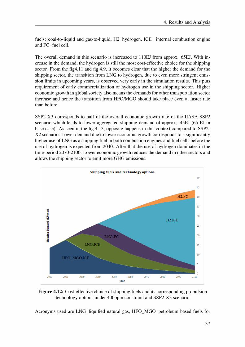
4. Results and Analysis

fuels: coal-to-liquid and gas-to-liquid, H2=hydrogen, ICE= internal combustion engineand FC=fuel cell.

The overall demand in this scenario is increased to 110EJ from approx. 65EJ. With in-crease in the demand, the hydrogen is still the most cost-effective choice for the shippingsector. From the fig4.11 and fig.4.9, it becomes clear that the higher the demand for theshipping sector, the transition from LNG to hydrogen, due to even more stringent emis-sion limits in upcoming years, is observed very early in the simulation results. This putsrequirement of early commercialization of hydrogen use in the shipping sector. Highereconomic growth in global society also means the demands for other transportation sectorincrease and hence the transition from HFO/MGO should take place even at faster ratethan before.

SSP2-X3 corresponds to half of the overall economic growth rate of the IIASA-SSP2scenario which leads to lower aggregated shipping demand of approx. 45EJ (65 EJ inbase case). As seen in the fig.4.13, opposite happens in this context compared to SSP2-X2 scenario. Lower demand due to lower economic growth corresponds to a significantlyhigher use of LNG as a shipping fuel in both combustion engines and fuel cells before theuse of hydrogen is expected from 2040. After that the use of hydrogen dominates in thetime-period 2070-2100. Lower economic growth reduces the demand in other sectors andallows the shipping sector to emit more GHG emissions.

Figure 4.12: Cost-effective choice of shipping fuels and its corresponding propulsiontechnology options under 400ppm constraint and SSP2-X3 scenario

Acronyms used are LNG=liquified natural gas, HFO_MGO=petroleum based fuels for

37

4. Results and Analysis

ships: heavy fuel oil (HFO) and marine gas oil (MGO), H2=hydrogen, ICE= internalcombustion engine and FC=fuel cell.

Comparing all the three demands in the three scenarios, it is indicated that the hydrogenis the expected cost-effective fuel choice in the shipping sector in longer term scenarioprovided with stringent CO2 constraints in the scenario about supply potentials of primaryenergy resources. Depending upon the level of demand in the marine shipping sector,the transition of alternative fuels is decided. As the demand increases, the transitionfrom HFO/MGO to LNG and then to hydrogen is expected at an early year and in afaster way. Methane leakage is very important factor when it comes to using the naturalgas in the shipping sector. More stringent emission limits results in more usage of fuelcell technology coupled to natural gas used to power the ships. Also, the use of energyconversion technology coupled with the use of hydrogen is dependent on the amount ofshipping demand. Observing the composition of future fuels to be used in the shippingsector by the end of this century against the level of demand, it is seen that the percentageof hydrogen coupled with fuel cell technology increases with increase in demand. Thishappens due to limited supply potentials of different primary resources such as oil andbio-energy etc. Overall, all the different results suggest how the level of demand is animportant variable which will affect the cost-effective choice of alternative shipping fuel.

4.6.2 Concerns Towards Hydrogen as A Marine Fuel

There are still concerns about hydrogen as an alternative fuel in the marine shipping sec-tor about safety issues, energy density and lack of infrastructure. As seen from the resultsuntil now in this study, hydrogen is expected to become an energy carrier which will in-crease the deep decarbonization efforts in the marine transportation sector at a minimumcost to the whole energy system. But Hydrogen requires larger space to store onboardthe ships. Even if it is kept under 700 bars pressure, there is a still requirement of sixtimes bigger storage space[42]. Lower energy density means more fuel consumption forthe same energy content provided by HFO. This results in even more space requirement.

Hydrogen propulsion is yet to be tested successfully in the marine shipping sector forlarge scale energy production. The advent of this unproven technology might be a slowprocess. Also, supply infrastructure is another concern which needs to be addressed. It iscommonly referred to as a “chicken-and-egg” problem. Some of these concerns reflect inuncertain mature commercial costs of using hydrogen as a shipping fuel. That’s why thesensitivity analysis is performed to understand which alternative and marine fuels helpthe shipping sector to reduce its emission when hydrogen is not a feasible option.

38

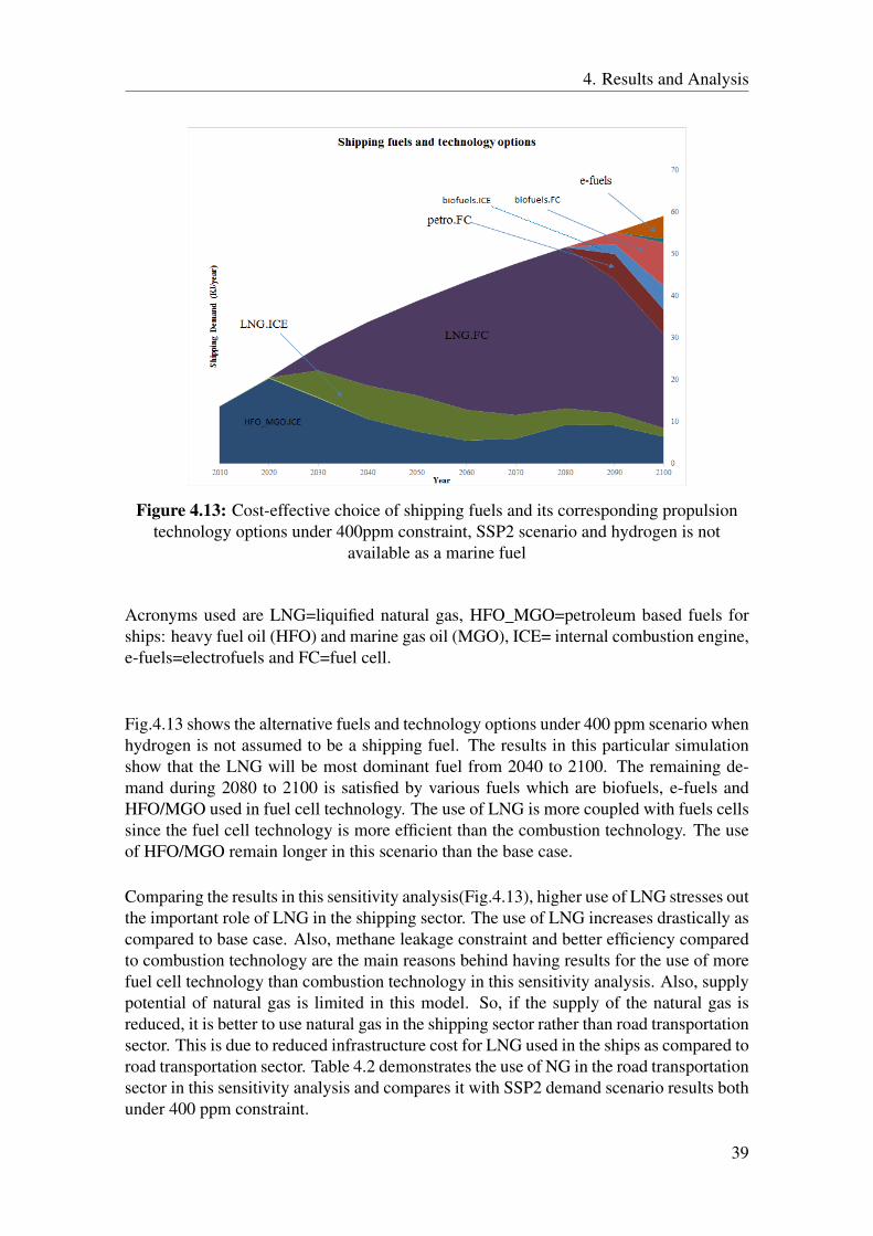
4. Results and Analysis

Figure 4.13: Cost-effective choice of shipping fuels and its corresponding propulsiontechnology options under 400ppm constraint, SSP2 scenario and hydrogen is not

available as a marine fuel

Acronyms used are LNG=liquified natural gas, HFO_MGO=petroleum based fuels forships: heavy fuel oil (HFO) and marine gas oil (MGO), ICE= internal combustion engine,e-fuels=electrofuels and FC=fuel cell.

Fig.4.13 shows the alternative fuels and technology options under 400 ppm scenario whenhydrogen is not assumed to be a shipping fuel. The results in this particular simulationshow that the LNG will be most dominant fuel from 2040 to 2100. The remaining de-mand during 2080 to 2100 is satisfied by various fuels which are biofuels, e-fuels andHFO/MGO used in fuel cell technology. The use of LNG is more coupled with fuels cellssince the fuel cell technology is more efficient than the combustion technology. The useof HFO/MGO remain longer in this scenario than the base case.

Comparing the results in this sensitivity analysis(Fig.4.13), higher use of LNG stresses outthe important role of LNG in the shipping sector. The use of LNG increases drastically ascompared to base case. Also, methane leakage constraint and better efficiency comparedto combustion technology are the main reasons behind having results for the use of morefuel cell technology than combustion technology in this sensitivity analysis. Also, supplypotential of natural gas is limited in this model. So, if the supply of the natural gas isreduced, it is better to use natural gas in the shipping sector rather than road transportationsector. This is due to reduced infrastructure cost for LNG used in the ships as compared toroad transportation sector. Table 4.2 demonstrates the use of NG in the road transportationsector in this sensitivity analysis and compares it with SSP2 demand scenario results bothunder 400 ppm constraint.

39

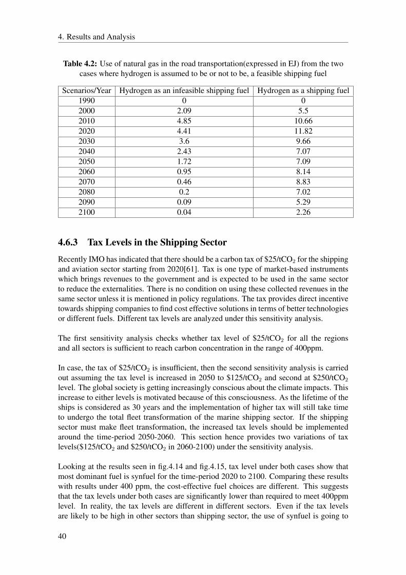
4. Results and Analysis

Table 4.2: Use of natural gas in the road transportation(expressed in EJ) from the twocases where hydrogen is assumed to be or not to be, a feasible shipping fuel

Scenarios/Year Hydrogen as an infeasible shipping fuel Hydrogen as a shipping fuel1990 0 02000 2.09 5.52010 4.85 10.662020 4.41 11.822030 3.6 9.662040 2.43 7.072050 1.72 7.092060 0.95 8.142070 0.46 8.832080 0.2 7.022090 0.09 5.292100 0.04 2.26

4.6.3 Tax Levels in the Shipping Sector

Recently IMO has indicated that there should be a carbon tax of $25/tCO2 for the shippingand aviation sector starting from 2020[61]. Tax is one type of market-based instrumentswhich brings revenues to the government and is expected to be used in the same sectorto reduce the externalities. There is no condition on using these collected revenues in thesame sector unless it is mentioned in policy regulations. The tax provides direct incentivetowards shipping companies to find cost effective solutions in terms of better technologiesor different fuels. Different tax levels are analyzed under this sensitivity analysis.

The first sensitivity analysis checks whether tax level of $25/tCO2 for all the regionsand all sectors is sufficient to reach carbon concentration in the range of 400ppm.

In case, the tax of $25/tCO2 is insufficient, then the second sensitivity analysis is carriedout assuming the tax level is increased in 2050 to $125/tCO2 and second at $250/tCO2level. The global society is getting increasingly conscious about the climate impacts. Thisincrease to either levels is motivated because of this consciousness. As the lifetime of theships is considered as 30 years and the implementation of higher tax will still take timeto undergo the total fleet transformation of the marine shipping sector. If the shippingsector must make fleet transformation, the increased tax levels should be implementedaround the time-period 2050-2060. This section hence provides two variations of taxlevels($125/tCO2 and $250/tCO2 in 2060-2100) under the sensitivity analysis.

Looking at the results seen in fig.4.14 and fig.4.15, tax level under both cases show thatmost dominant fuel is synfuel for the time-period 2020 to 2100. Comparing these resultswith results under 400 ppm, the cost-effective fuel choices are different. This suggeststhat the tax levels under both cases are significantly lower than required to meet 400ppmlevel. In reality, the tax levels are different in different sectors. Even if the tax levelsare likely to be high in other sectors than shipping sector, the use of synfuel is going to

40

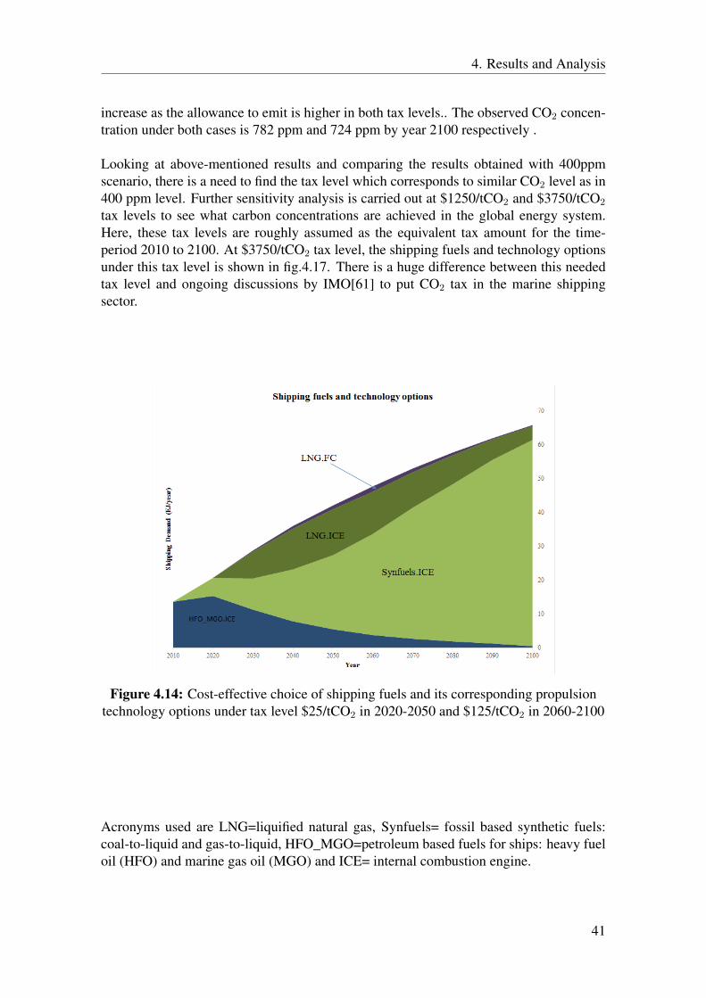
4. Results and Analysis

increase as the allowance to emit is higher in both tax levels.. The observed CO2 concen-tration under both cases is 782 ppm and 724 ppm by year 2100 respectively .

Looking at above-mentioned results and comparing the results obtained with 400ppmscenario, there is a need to find the tax level which corresponds to similar CO2 level as in400 ppm level. Further sensitivity analysis is carried out at $1250/tCO2 and $3750/tCO2tax levels to see what carbon concentrations are achieved in the global energy system.Here, these tax levels are roughly assumed as the equivalent tax amount for the time-period 2010 to 2100. At $3750/tCO2 tax level, the shipping fuels and technology optionsunder this tax level is shown in fig.4.17. There is a huge difference between this neededtax level and ongoing discussions by IMO[61] to put CO2 tax in the marine shippingsector.

Figure 4.14: Cost-effective choice of shipping fuels and its corresponding propulsiontechnology options under tax level $25/tCO2 in 2020-2050 and $125/tCO2 in 2060-2100

Acronyms used are LNG=liquified natural gas, Synfuels= fossil based synthetic fuels:coal-to-liquid and gas-to-liquid, HFO_MGO=petroleum based fuels for ships: heavy fueloil (HFO) and marine gas oil (MGO) and ICE= internal combustion engine.

41

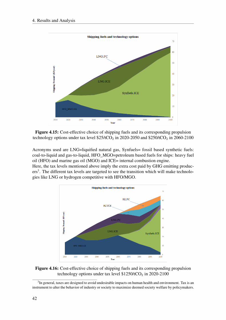
4. Results and Analysis

Figure 4.15: Cost-effective choice of shipping fuels and its corresponding propulsiontechnology options under tax level $25/tCO2 in 2020-2050 and $250/tCO2 in 2060-2100

Acronyms used are LNG=liquified natural gas, Synfuels= fossil based synthetic fuels:coal-to-liquid and gas-to-liquid, HFO_MGO=petroleum based fuels for ships: heavy fueloil (HFO) and marine gas oil (MGO) and ICE= internal combustion engine.Here, the tax levels mentioned above imply the extra cost paid by GHG emitting produc-ers3. The different tax levels are targeted to see the transition which will make technolo-gies like LNG or hydrogen competitive with HFO/MGO.

Figure 4.16: Cost-effective choice of shipping fuels and its corresponding propulsiontechnology options under tax level $1250/tCO2 in 2020-2100

3In general, taxes are designed to avoid undesirable impacts on human health and environment. Tax is aninstrument to alter the behavior of industry or society to maximize deemed society welfare by policymakers.

42

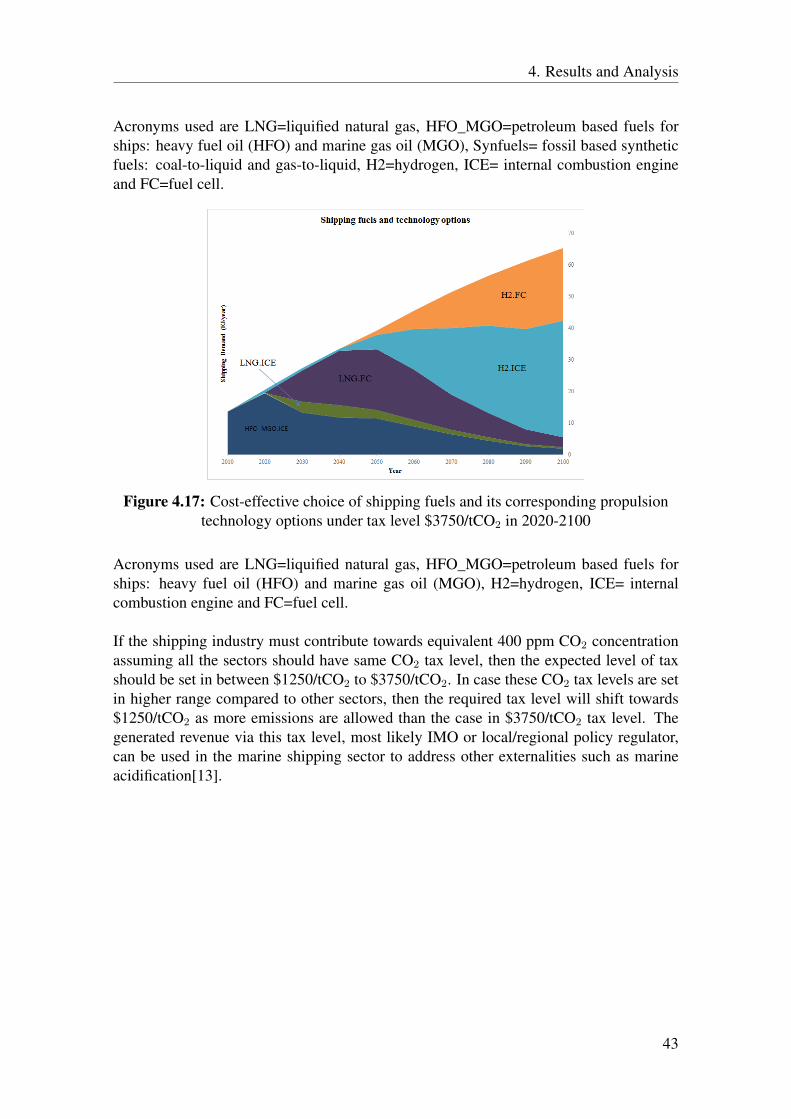
4. Results and Analysis

Acronyms used are LNG=liquified natural gas, HFO_MGO=petroleum based fuels forships: heavy fuel oil (HFO) and marine gas oil (MGO), Synfuels= fossil based syntheticfuels: coal-to-liquid and gas-to-liquid, H2=hydrogen, ICE= internal combustion engineand FC=fuel cell.

Figure 4.17: Cost-effective choice of shipping fuels and its corresponding propulsiontechnology options under tax level $3750/tCO2 in 2020-2100

Acronyms used are LNG=liquified natural gas, HFO_MGO=petroleum based fuels forships: heavy fuel oil (HFO) and marine gas oil (MGO), H2=hydrogen, ICE= internalcombustion engine and FC=fuel cell.

If the shipping industry must contribute towards equivalent 400 ppm CO2 concentrationassuming all the sectors should have same CO2 tax level, then the expected level of taxshould be set in between $1250/tCO2 to $3750/tCO2. In case these CO2 tax levels are setin higher range compared to other sectors, then the required tax level will shift towards$1250/tCO2 as more emissions are allowed than the case in $3750/tCO2 tax level. Thegenerated revenue via this tax level, most likely IMO or local/regional policy regulator,can be used in the marine shipping sector to address other externalities such as marineacidification[13].

43

4. Results and Analysis

44

5Discussion and Conclusion

The results obtained from the GET model suggest that the cost-effective choices in the ma-rine shipping sector require a transition beginning in 2010 from HFO/MGO to methanol/L-NG/hydrogen in different scenario analysis. Even in BAU scenario, the cost-effectivechoices suggest transition beginning in 2010 and 2020 from HFO/MGO to methanol andLNG respectively. This is because of the limited supply potentials of oil reserves. Thesealternate fuels used in the marine shipping sector in BAU scenario only use already provenand cheap combustion technology. Also this combustion technology is already being usedin all the continents of the world and unclear incentives towards the shipping industrymight generate technology lock-in situation.

In a 400 ppm scenario, the cost-effective choices suggest LNG as a transitional fuel andhydrogen as the longer term marine renewable fuel for the shipping sector. Also, thesechoices suggest the use of more efficient fuel cells. As mentioned before the technologydispersion of the combustion technology makes it hard to get implemented everywhereat the same time. Policymakers need to create incentives for the shipping investors toinvest in this technology. In addition, these incentives must be created soon in order totransform the shipping fleet. To make this transformation happen, the IMO must start pro-viding information about long term plans and expected policy measures in future. Moreand clearer information about emissions will help IMO to design policies in a better way.This will also help the investors to set their own environmental goal as well as take intoaccount upcoming policies[62].

The results also conclude that the level of the shipping demand (expressed in EJ) playsvery important role in deciding the role of different technologies coupled to the use ofrenewable fuels, specifically in case of hydrogen. The higher the shipping demand, themore use of fuel cells is expected as per cost-effective solution, specifically as the ship-ping demand rises above 40EJ. Particularly both the fuel cell technology and hydrogencosts are very uncertain and not proven in the marine shipping sector. In short-term, thefocus should be to address this issue of commercialization as early as possible. Not onlyhigher demand suggests the additional use of hydrogen with fuel cells and limit the useof combustion engines with hydrogen but also suggest a quick and early transition to hy-drogen beginning in 2040.

The costs for hydrogen storage plays an important role in the marine shipping sector.It is expected that the use of hydrogen will take place first in the road transportation sec-tor and then the technology may become commercial in the shipping sector. The progressneeds to be faster by identifying more niche markets for hydrogen such as submarines

45

5. Discussion and Conclusion

and military ships and bring down costs for hydrogen storage. More investment in nichemarkets will bring down costs for hydrogen storage as well as technology expertise easesthe use in the shipping sector.

In order to make hydrogen competitive, there is a huge difference between the IMO dis-cussed tax level[61] and the needed tax level. This difference sends rather unwanted signaltowards shipping industry in a longer term. During the time-period when SOx and NOx

policies implementation took place, the industry favored using scrubber technology whensufficient incentives were present to start transition towards LNG as a marine fuel. Thisshowed a situation where a major part of industry refused to undergo fuel transformationwhen the incentives were present. Taking into consideration such kind of situations, it isbetter to create incentives for hydrogen as early as possible. This will help to address afterimplementation issues.

In case the shipping industry starts considering hydrogen to be an infeasible solution dueto cost of implementation or security concerns, then LNG (to a greater extent), bio-fuels,e-fuels and oil based fuels coupled with fuel cells are the cost effective choices for theshipping sector. The use of natural gas seems to be a very important and best possible usein the marine shipping sector.

To conclude, cost-effective solutions for the shipping transport sector suggest the useof hydrogen and LNG as the future alternative and renewable marine fuels. Both solu-tions are a way forward to the shipping sector rather picking one solution. To increase thediffusion of these fuels in the shipping sector, the energy infrastructure is another aspectthat needs to be addressed. Policymakers, could start making regulations, for examplesubsidies, which will set up the infrastructure for hydrogen and LNG refueling stations.

46

6Future Work

Following ideas are identified during the thesis work:• Improved information about technology investment cost for every category would

be beneficial for the analyses.

• Concrete information about feasibility of different fuels and corresponding propul-sion technology options in different shipping categories would provide more de-tailed analyses.

• Advanced information about technical configuration of ships and their average sizeswill increase the reliability of fleet number for every shipping category.

• In depth information about energy supply potentials in different regions would bebeneficial for detailed understanding of global energy system dynamics.

• Technology commercialization and dispersion varies in different regions. If possi-ble, this can improve the results for different sensitivity analysis.

• If possible, technology learning index can be added to efficiency values to improvethe overall results for cost-effective fuel choices.

47

6. Future Work

48

Bibliography

[1] R. K. Pachauri, Climate Change 2014 Synthesis Report. IPCC, 2014.[2] W. N. Adger, Fairness in adaptation to climate change. MIT press, 2006.[3] T. W. P. Smith, J. P. Jalkanen, B. A. Anderson, J. J. Corbett, J. Faber, S. Hanayama,

E. O’Keeffe, S. Parker, L. Johansson, L. Aldous, C. Raucci, M. Traut, S. Ettinger,D. Nelissen, D. S. Lee, S. Ng, A. Agrawal, J. J. Winebrake, and A. Hoen, M., “ThirdIMO Greenhouse Gas Study 2014,” International Maritime Organization (IMO), p.327, 2014.

[4] M. Cames, J. Graichen, A. Siemons, and V. Cook, “Emission Reduction Targets forInternational Aviation and Shipping,” Tech. Rep. 9, 2015.

[5] M. Taljegard, S. Brynolf, M. Grahn, K. Andersson, and H. Johnson, “Cost-EffectiveChoices of Marine Fuels in a Carbon-Constrained World : Results from a GlobalEnergy Model,” Environmetal Science and Technology, vol. 46, no. 21, pp. 12 986–12 993, 2014.

[6] S. Arrhenius, “in the Air upon the Temperature of the Ground,” Philosophocal Mag-azine and Journal of Science, vol. 41, no. page 270, pp. 237–279, 1896.

[7] J. Leggett, W. J. Pepper, R. J. Swart, J. Edmonds, L. G. Meira Filho, I. Mintzer,M. X. Wang, and J. Wasson, “Emissions scenarios for the IPCC: an update,” inClimate change 1992: the supplementary report to the IPCC scientific assessment,1992, pp. 69–95.

[8] “Summary for Policymakers,” IPCC, pp. 1–37, 2000.[9] R. H. Moss, J. A. Edmonds, K. A. Hibbard, M. R. Manning, S. K. Rose, D. P.

van Vuuren, T. R. Carter, S. Emori, M. Kainuma, T. Kram, G. A. Meehl, J. F. B.Mitchell, N. Nakice-novic, K. Riahi, S. J. Smith, R. J. Stouffer, A. M. Thomson, J. P.Weyant, T. J. Wilbanks, and N. Nakicenovic, “The next generation of scenarios forclimate change research and assessment,” Nature, vol. 463, no. 7282, pp. 747–756,2010. [Online]. Available: http://www.ncbi.nlm.nih.gov/pubmed/20148028

[10] B. C. O’Neill, E. Kriegler, K. L. Ebi, E. Kemp-Benedict, K. Riahi, D. S. Rothman,B. J. van Ruijven, D. P. van Vuuren, J. Birkmann, K. Kok, M. Levy, and W. Solecki,“The roads ahead: Narratives for shared socioeconomic pathways describing worldfutures in the 21st century,” Global Environmental Change, vol. 42, pp. 169–180,2014. [Online]. Available: http://dx.doi.org/10.1016/j.gloenvcha.2015.01.004

[11] V. Eyring, H. W. Köhler, A. Lauer, and B. Lemper, “Emissions from internationalshipping: 2. Impact of future technologies on scenarios until 2050,” Journal of Geo-physical Research D: Atmospheres, vol. 110, no. 17, pp. 183–200, 2005.

[12] Ø. Buhaug, J. J. Corbett, O. Endresen, V. Eyring, J. Faber, S. Hanayama, D. S. Lee,H. Lindstad, A. Markowska, A. Mjelde, D. Nelissen, J. Nilsen, C. Pålsson, J. J.

49

Bibliography

Winebrake, W. Wu, and K. Yoshida, “Study 2009,” International Maritime Organi-zation, London, Tech. Rep., 2009.

[13] O. Endresen, M. Eide, S. Dalsoren, I. Isaksen, and E. Sorgard, “The EnvironmentalImpacts of Increased International Maritime Shipping,” Global Forum on Transportand Environment in a Globalising World, no. November, pp. 1–43, 2008.

[14] J. J. Corbett, C. Wang, J. J. Winebrake, and E. Green, “Allocation and forecasting ofglobal ship emissions,” Clean Air Task Force, Boston, MA, USA, Tech. Rep. August2015, 2007.

[15] K. L. Ebi, S. Hallegatte, T. Kram, N. W. Arnell, T. R. Carter, J. Edmonds, E. Kriegler,R. Mathur, B. C. O’Neill, K. Riahi, H. Winkler, D. P. van Vuuren, and T. Zwickel,“A new scenario framework for climate change research: Background, process, andfuture directions,” Climatic Change, vol. 122, no. 3, pp. 363–372, 2014.

[16] Ocean Policy Research Foundation, “The World’s Changing Maritime Industry anda Vision for Japan,” Ocean Policy Research Foundation (OPRF), Tech. Rep., 2008.

[17] C. C. Chang, “Marine energy consumption, national economic activity, and green-house gas emissions from international shipping,” Energy Policy, vol. 41, pp. 843–848, 2012.

[18] J. Vergara, C. McKesson, and M. Walczak, “Sustainable energy for themarine sector,” Energy Policy, vol. 49, pp. 333–345, 2012. [Online]. Available:http://dx.doi.org/10.1016/j.enpol.2012.06.026

[19] K. Riahi, D. P. V. Vuuren, E. Kriegler, J. Edmonds, B. C. O. Neill, S. Fujimori,N. Bauer, K. Calvin, R. Dellink, O. Fricko, W. Lutz, A. Popp, J. Crespo, S. Kc,M. Leimbach, L. Jiang, T. Kram, S. Rao, J. Emmerling, K. Ebi, T. Hasegawa,P. Havlik, F. Humpenöder, L. Aleluia, D. Silva, S. Smith, E. Stehfest, V. Bosetti,J. Eom, D. Gernaat, T. Masui, J. Rogelj, J. Stre, L. Drouet, V. Krey, G. Luderer,M. Harmsen, K. Takahashi, L. Baumstark, J. C. Doelman, M. Kainuma, Z. Klimont,G. Marangoni, H. Lotze-campen, M. Obersteiner, A. Tabeau, and M. Tavoni, “TheShared Socioeconomic Pathways and their energy , land use , and greenhouse gasemissions implications : An overview,” vol. 42, pp. 153–168, 2017.

[20] “Towards new scenarios for analysis of emissions, climate chage impacts and re-sponse strategies,” IPCC, 2007.

[21] P. Agnolucci, N. J. Lazarou, S. Mander, and C. Walsh, “Shipping Demand ScenariosUsing Estimated Elasticities,” in Shipping in Changing Climates Conference 2015,2015.

[22] M. Traut, S. Hanson, and C. Walsh, “Report from the lookout Understanding climatechange impacts on shipping,” no. November, pp. 10–11, 2016.

[23] R. Schuitmaker, “Evolution of Global Maritime Freight Energy demand and co2emissions: A BAU and 2DS Scenario,” vol. 2016, no. November, p. 69, 2016.

[24] C. Raucci, C. Walsh, J. Calleya, M. Traut, N. Smith, S. De la Fuente, S. Haji, andT. Smith, “Low carbon pathways,” Lloyd’s Register, Tech. Rep. June, 2015.

[25] A. F. Friedlaender and R. H. Spady, “A derived demand function for freighttransportation,” The Review of Economics and Statistics, vol. 62, no. 3, pp.432–441, 1980. [Online]. Available: http://www.jstor.org/stable/1927111

[26] UNCTAD, “Review of Maritime Transport 2016,” in United Nations Conferenceon Trade and Development. Geneva, Switzerland: United Nations Conference onTrade and Development, 2016.

50

Bibliography

[27] M. Cropper and C. Griffiths, “The interaction of population growth andenvironmental quality,” The American Economic Review, vol. 84, no. 2, pp.250–254, 1994. [Online]. Available: http://www.jstor.org/stable/2117838

[28] I. T. F. T. Outlook, ITF Transport Outlook 2015, 2015. [Online]. Available: http://www.oecd-ilibrary.org/transport/itf-transport-outlook-2015_9789282107782-en

[29] Exergia, “Study on Clean Transport Systems Project 2010 n . 419-1-Unit Move B4Multiple Framework Services Contract with reopened competition for Technical As-sistance,” European Commission, Directorate-General for Mobility and Transport,no. November, p. 248, 2011.

[30] “Review of Maritime Transport 2015,” in United Nations Conference on Trade andDevelopment, no. October, 2015, p. 204.

[31] M. S. Andersen, “An introductory note on the environmental economics of the cir-cular economy,” pp. 133–140, 2007.

[32] Y. Kou and M. Luo, “Strategic capacity competition and overcapacity in shipping,”Maritime Policy & Management, vol. 43, no. 4, pp. 389–406, 2016.

[33] S. Schlott, “Large Engine Building Complexity Soars,” MTZ worldwide,vol. 78, no. 3, pp. 8–15, 2017. [Online]. Available: http://dx.doi.org/10.1007/s38313-017-0017-x

[34] J. J. Corbett, H. Wang, and J. J. Winebrake, “The effectiveness and costsof speed reductions on emissions from international shipping,” TransportationResearch Part D, vol. 14, no. 8, pp. 593–598, 2009. [Online]. Available:http://dx.doi.org/10.1016/j.trd.2009.08.005

[35] MAN Primeserv, “Slow Steaming Practices in the Global Shipping Industry,” Tech.Rep., 2012.

[36] “Review of Maritime Transport 2013,” in United Nations Conference on Trade andDevelopment, 2013.

[37] J. Wismans, M. Grahn, and I. Denbratt, “Low-carbon transport–health and climatebenefits,” in Background report to UNRCD Intergovernmental Ninth Regional En-vironmentally Sustainable Transport (EST) Forum in Asia. Chalmers University ofTechnology, 2016.

[38] J. Gravina, J. I. R. Blake, P. A. Shenoi, P. S. Turnock, and S. Hirdaris, “Concepts fora Modular Nuclear Powered Containership,” 2007.

[39] K. Juoperi, “Heavy fuel oil- still the dominent fuel quality for diesel engines,” 2005.[40] OECD, “Environmental Impacts of International Shipping: The Role of Ports,”

OECD Publishing, Paris, Tech. Rep., 2011.[41] N. Molloy, “ The IMO’s global sulfur cap: What a 2020 sulfur constrained world

means for shipping lines, refineries and bunker suppliers,” S&P Global, Tech. Rep.October, 2016.

[42] C. Azar, K. Lindgren, and B. Andersson, “Hydrogen or methanol in the transporta-tion sector?” Tech. Rep. i, 2000.

[43] F. Mosheni, “Power to gas – bridging renewable electricity to the transport sector,”KTH Royal Institute of Technology, Stockholm, 2012.

[44] E. Parson, V. Burkett, K. Fisher-Vanden, D. Keith, L. Mearns, H. Pitcher,C. Rosenzweig, and M. Webster, “Global-change Scenarios: Their Developmentand Use,” US Department of Energy Publications, vol. 7, no. July, p. 7, 2007.

51

Bibliography

[Online]. Available: http://www.climatescience.gov/Library/sap/sap2-1/finalreport/sap2-1b-final-authors.pdf

[45] O. Fricko, P. Havlik, J. Rogelj, Z. Klimont, M. Gusti, N. Johnson, P. Kolp,M. Strubegger, H. Valin, M. Amann, T. Ermolieva, N. Forsell, M. Herrero,C. Heyes, G. Kindermann, V. Krey, D. L. McCollum, M. Obersteiner, S. Pachauri,S. Rao, E. Schmid, W. Schoepp, and K. Riahi, “The marker quantification of theShared Socioeconomic Pathway 2: A middle-of-the-road scenario for the 21stcentury,” Global Environmental Change, vol. 42, pp. 251–267, 2015. [Online].Available: http://dx.doi.org/10.1016/j.gloenvcha.2016.06.004

[46] A. Andersson, C. Azar, and K. Lindgren, “Global energy scenarios meeting stringentCO2 constraints— Cost-effective fuel choices in the transportation sector,” EnergyPolicy, vol. 31, pp. 961–976, 2003.

[47] M. Grahn, S. Brynolf, J. Hansson, and M. Taljegard, “The cost-effectiveness ofelectrofuels in comparison to other alternative fuels for transport in a low carbonfuture,” in European Biomass Conference and Exhibition, 2016, pp. 6–9.

[48] “Review of Maritime transport 2003,” in United Nations Conference onTrade and Development. United Nations, 2003. [Online]. Available: http://unctad.org/en/Docs/rmt2003_en.pdf

[49] “The world merchant fleet in 2015 Statistics from Equasis,” European MaritimeSafety Assessment, Tech. Rep., 2015.

[50] “The world merchant fleet in 2010 Statistics from Equasis,” European MaritimeSafety Assessment, Tech. Rep., 2010.

[51] “The world merchant fleet in 2010 Statistics from Equasis,” European MaritimeSafety Assessment, Tech. Rep., 2005.

[52] “SSP Database 2017. [Online].Available: https://tntcat.iiasa.ac.at/SspDb/dsd?Action=htmlpage&page=series. [Ac-cessed: 20- Mar- 2017].”

[53] T. Wigley, R. Richels, and J. Edmonds, “Economic and Environmental choices inthe stabilization of atmospheric co2 concentrations,” Letters to Nature, vol. 379,1996. [Online]. Available: https://www.nature.com/nature/journal/v379/n6562/pdf/379240a0.pdf

[54] M. Grahn, Cost-effective fuel and technology choices in the transportation sector ina future carbon constrained world, phd thesis ed. Gothenburg: Chalmers Universityof Technology, 2009.

[55] F. Hedenus, S. Karlsson, C. Azar, and F. Sprei, “Cost-effective energy carriers fortransport – The role of the energy supply system in a carbon-constrained world,”International Journal of Hydrogen Energy, vol. 35, no. 10, pp. 4638–4651, 2010.[Online]. Available: http://dx.doi.org/10.1016/j.ijhydene.2010.02.064

[56] T. Malthus, “An Essay on the Principle of Population,” London, Tech. Rep., 1998.[57] I. F. Crespo and T. D. If, “Income projections for climate change research : A frame-

work based on human capital dynamics §,” vol. 42, pp. 226–236, 2017.[58] R. Dellink, J. Chateau, E. Lanzi, and B. Magne, “Long-term economic growth pro-

jections in the Shared Socioeconomic Pathways §,” vol. 42, pp. 200–214, 2017.[59] M. Leimbach, E. Kriegler, N. Roming, and J. Schwanitz, “Future growth patterns of

world regions – A GDP scenario approach,” Global Environmental Change, vol. 42,

52

Bibliography

pp. 215–225, 2017. [Online]. Available: http://dx.doi.org/10.1016/j.gloenvcha.2015.02.005

[60] I. P. on Climate Change, Climate Change 2014–Impacts, Adaptation and Vulnera-bility: Regional Aspects. Cambridge University Press, 2014.

[61] “Market-Based Instruments for International Aviation and Shipping as a Source ofClimate Finance,” International Monetary Fund and World Bank, no. November,2011.

[62] M. Mahmudur, T. Islam, and S. Kuruppu, “Regulating global shipping corporations’ accountability for reducing greenhouse gas emissions in the seas,” vol. 69, pp.159–170, 2016.

53

Bibliography

54

AAppendix 1

Table A.1: Estimated Population in IIASA-SSP2 Scenario

Final Population Count (Gpeople)Year 1990 2000 2010 2020 2030 2040 2050 2060 2070 2080 2090 2100NAM 2.87E-01 3.20E-01 3.48E-01 3.77E-01 4.06E-01 4.31E-01 4.53E-01 4.74E-01 4.93E-01 5.06E-01 5.13E-01 5.15E-01EUR 5.57E-01 5.80E-01 6.02E-01 6.26E-01 6.45E-01 6.58E-01 6.66E-01 6.68E-01 6.64E-01 6.55E-01 6.42E-01 6.25E-01PAO 1.87E-01 1.97E-01 2.01E-01 2.05E-01 2.05E-01 2.02E-01 1.97E-01 1.90E-01 1.83E-01 1.74E-01 1.64E-01 1.54E-01FSU 2.90E-01 2.90E-01 2.86E-01 2.88E-01 2.87E-01 2.85E-01 2.83E-01 2.79E-01 2.73E-01 2.65E-01 2.56E-01 2.46E-01LAM 4.38E-01 5.16E-01 5.85E-01 6.44E-01 6.91E-01 7.24E-01 7.42E-01 7.44E-01 7.35E-01 7.18E-01 6.95E-01 6.70E-01MEA 2.76E-01 3.43E-01 4.24E-01 5.06E-01 5.79E-01 6.43E-01 6.95E-01 7.31E-01 7.51E-01 7.58E-01 7.55E-01 7.44E-01AFR 4.80E-01 6.22E-01 8.12E-01 1.02E+00 1.25E+00 1.48E+00 1.70E+00 1.88E+00 2.04E+00 2.17E+00 2.25E+00 2.31E+00CPA 1.28E+00 1.43E+00 1.48E+00 1.54E+00 1.55E+00 1.51E+00 1.43E+00 1.33E+00 1.22E+00 1.10E+00 9.94E-01 9.00E-01PAS 3.66E-01 4.32E-01 4.94E-01 5.46E-01 5.87E-01 6.14E-01 6.26E-01 6.26E-01 6.15E-01 5.97E-01 5.74E-01 5.48E-01SAS 1.12E+00 1.36E+00 1.63E+00 1.86E+00 2.07E+00 2.24E+00 2.37E+00 2.45E+00 2.47E+00 2.44E+00 2.38E+00 2.29E+00

Global 5.28E+00 6.09E+00 6.87E+00 7.61E+00 8.26E+00 8.78E+00 9.16E+00 9.37E+00 9.44E+00 9.38E+00 9.22E+00 9.00E+00

I

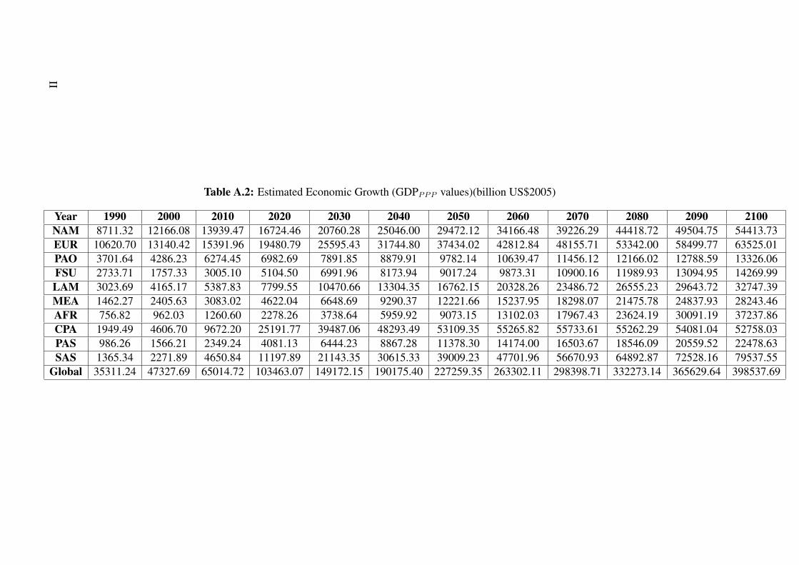
Table A.2: Estimated Economic Growth (GDPP P P values)(billion US$2005)

Year 1990 2000 2010 2020 2030 2040 2050 2060 2070 2080 2090 2100NAM 8711.32 12166.08 13939.47 16724.46 20760.28 25046.00 29472.12 34166.48 39226.29 44418.72 49504.75 54413.73EUR 10620.70 13140.42 15391.96 19480.79 25595.43 31744.80 37434.02 42812.84 48155.71 53342.00 58499.77 63525.01PAO 3701.64 4286.23 6274.45 6982.69 7891.85 8879.91 9782.14 10639.47 11456.12 12166.02 12788.59 13326.06FSU 2733.71 1757.33 3005.10 5104.50 6991.96 8173.94 9017.24 9873.31 10900.16 11989.93 13094.95 14269.99LAM 3023.69 4165.17 5387.83 7799.55 10470.66 13304.35 16762.15 20328.26 23486.72 26555.23 29643.72 32747.39MEA 1462.27 2405.63 3083.02 4622.04 6648.69 9290.37 12221.66 15237.95 18298.07 21475.78 24837.93 28243.46AFR 756.82 962.03 1260.60 2278.26 3738.64 5959.92 9073.15 13102.03 17967.43 23624.19 30091.19 37237.86CPA 1949.49 4606.70 9672.20 25191.77 39487.06 48293.49 53109.35 55265.82 55733.61 55262.29 54081.04 52758.03PAS 986.26 1566.21 2349.24 4081.13 6444.23 8867.28 11378.30 14174.00 16503.67 18546.09 20559.52 22478.63SAS 1365.34 2271.89 4650.84 11197.89 21143.35 30615.33 39009.23 47701.96 56670.93 64892.87 72528.16 79537.55

Global 35311.24 47327.69 65014.72 103463.07 149172.15 190175.40 227259.35 263302.11 298398.71 332273.14 365629.64 398537.69

II

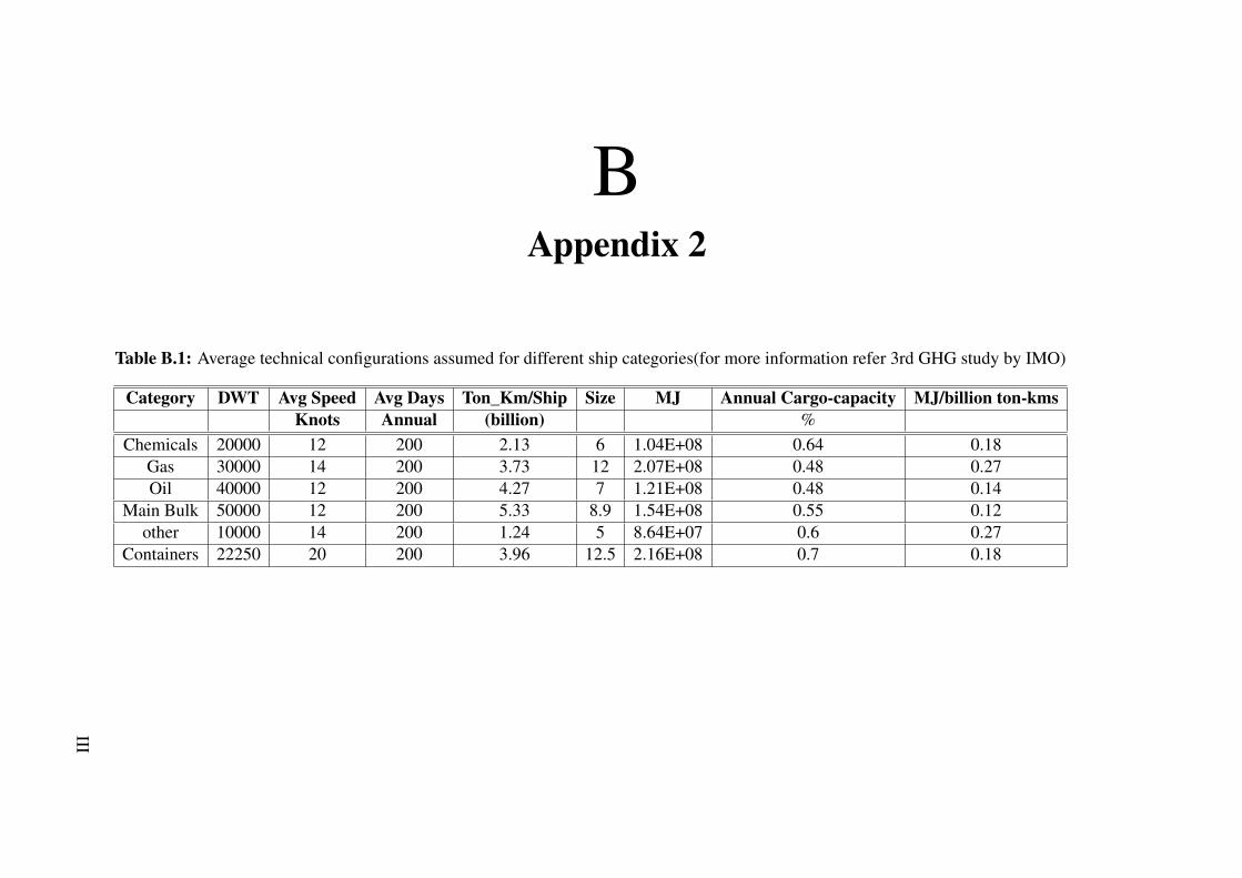
BAppendix 2

Table B.1: Average technical configurations assumed for different ship categories(for more information refer 3rd GHG study by IMO)

Category DWT Avg Speed Avg Days Ton_Km/Ship Size MJ Annual Cargo-capacity MJ/billion ton-kmsKnots Annual (billion) %

Chemicals 20000 12 200 2.13 6 1.04E+08 0.64 0.18Gas 30000 14 200 3.73 12 2.07E+08 0.48 0.27Oil 40000 12 200 4.27 7 1.21E+08 0.48 0.14

Main Bulk 50000 12 200 5.33 8.9 1.54E+08 0.55 0.12other 10000 14 200 1.24 5 8.64E+07 0.6 0.27

Containers 22250 20 200 3.96 12.5 2.16E+08 0.7 0.18

III

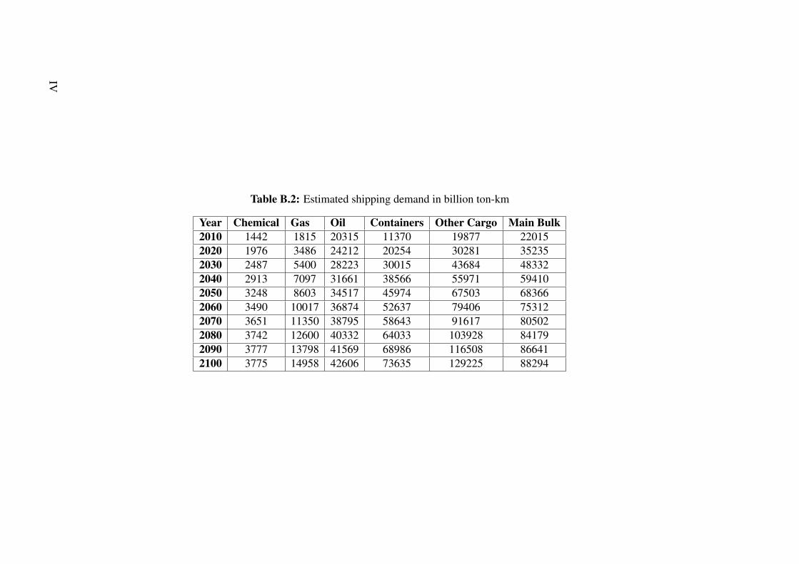
Table B.2: Estimated shipping demand in billion ton-km

Year Chemical Gas Oil Containers Other Cargo Main Bulk2010 1442 1815 20315 11370 19877 220152020 1976 3486 24212 20254 30281 352352030 2487 5400 28223 30015 43684 483322040 2913 7097 31661 38566 55971 594102050 3248 8603 34517 45974 67503 683662060 3490 10017 36874 52637 79406 753122070 3651 11350 38795 58643 91617 805022080 3742 12600 40332 64033 103928 841792090 3777 13798 41569 68986 116508 866412100 3775 14958 42606 73635 129225 88294

IV

CAppendix 3

V

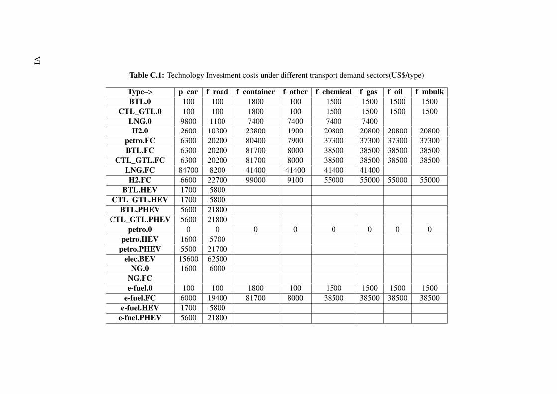
Table C.1: Technology Investment costs under different transport demand sectors(US$/type)

Type–> p_car f_road f_container f_other f_chemical f_gas f_oil f_mbulkBTL.0 100 100 1800 100 1500 1500 1500 1500

CTL_GTL.0 100 100 1800 100 1500 1500 1500 1500LNG.0 9800 1100 7400 7400 7400 7400H2.0 2600 10300 23800 1900 20800 20800 20800 20800

petro.FC 6300 20200 80400 7900 37300 37300 37300 37300BTL.FC 6300 20200 81700 8000 38500 38500 38500 38500

CTL_GTL.FC 6300 20200 81700 8000 38500 38500 38500 38500LNG.FC 84700 8200 41400 41400 41400 41400H2.FC 6600 22700 99000 9100 55000 55000 55000 55000

BTL.HEV 1700 5800CTL_GTL.HEV 1700 5800

BTL.PHEV 5600 21800CTL_GTL.PHEV 5600 21800

petro.0 0 0 0 0 0 0 0 0petro.HEV 1600 5700

petro.PHEV 5500 21700elec.BEV 15600 62500

NG.0 1600 6000NG.FCe-fuel.0 100 100 1800 100 1500 1500 1500 1500

e-fuel.FC 6000 19400 81700 8000 38500 38500 38500 38500e-fuel.HEV 1700 5800

e-fuel.PHEV 5600 21800

VI

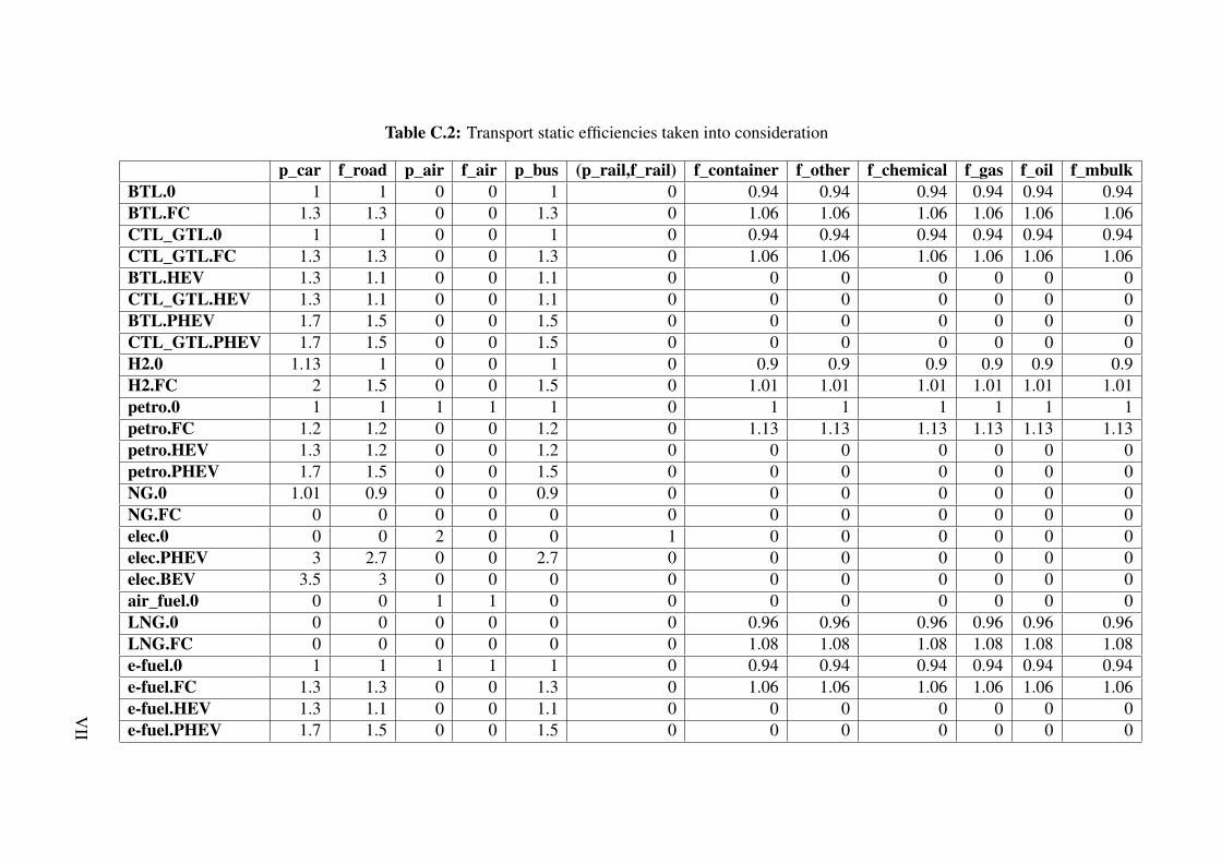
Table C.2: Transport static efficiencies taken into consideration

p_car f_road p_air f_air p_bus (p_rail,f_rail) f_container f_other f_chemical f_gas f_oil f_mbulkBTL.0 1 1 0 0 1 0 0.94 0.94 0.94 0.94 0.94 0.94BTL.FC 1.3 1.3 0 0 1.3 0 1.06 1.06 1.06 1.06 1.06 1.06CTL_GTL.0 1 1 0 0 1 0 0.94 0.94 0.94 0.94 0.94 0.94CTL_GTL.FC 1.3 1.3 0 0 1.3 0 1.06 1.06 1.06 1.06 1.06 1.06BTL.HEV 1.3 1.1 0 0 1.1 0 0 0 0 0 0 0CTL_GTL.HEV 1.3 1.1 0 0 1.1 0 0 0 0 0 0 0BTL.PHEV 1.7 1.5 0 0 1.5 0 0 0 0 0 0 0CTL_GTL.PHEV 1.7 1.5 0 0 1.5 0 0 0 0 0 0 0H2.0 1.13 1 0 0 1 0 0.9 0.9 0.9 0.9 0.9 0.9H2.FC 2 1.5 0 0 1.5 0 1.01 1.01 1.01 1.01 1.01 1.01petro.0 1 1 1 1 1 0 1 1 1 1 1 1petro.FC 1.2 1.2 0 0 1.2 0 1.13 1.13 1.13 1.13 1.13 1.13petro.HEV 1.3 1.2 0 0 1.2 0 0 0 0 0 0 0petro.PHEV 1.7 1.5 0 0 1.5 0 0 0 0 0 0 0NG.0 1.01 0.9 0 0 0.9 0 0 0 0 0 0 0NG.FC 0 0 0 0 0 0 0 0 0 0 0 0elec.0 0 0 2 0 0 1 0 0 0 0 0 0elec.PHEV 3 2.7 0 0 2.7 0 0 0 0 0 0 0elec.BEV 3.5 3 0 0 0 0 0 0 0 0 0 0air_fuel.0 0 0 1 1 0 0 0 0 0 0 0 0LNG.0 0 0 0 0 0 0 0.96 0.96 0.96 0.96 0.96 0.96LNG.FC 0 0 0 0 0 0 1.08 1.08 1.08 1.08 1.08 1.08e-fuel.0 1 1 1 1 1 0 0.94 0.94 0.94 0.94 0.94 0.94e-fuel.FC 1.3 1.3 0 0 1.3 0 1.06 1.06 1.06 1.06 1.06 1.06e-fuel.HEV 1.3 1.1 0 0 1.1 0 0 0 0 0 0 0e-fuel.PHEV 1.7 1.5 0 0 1.5 0 0 0 0 0 0 0

VII

C. Appendix 3

VIII

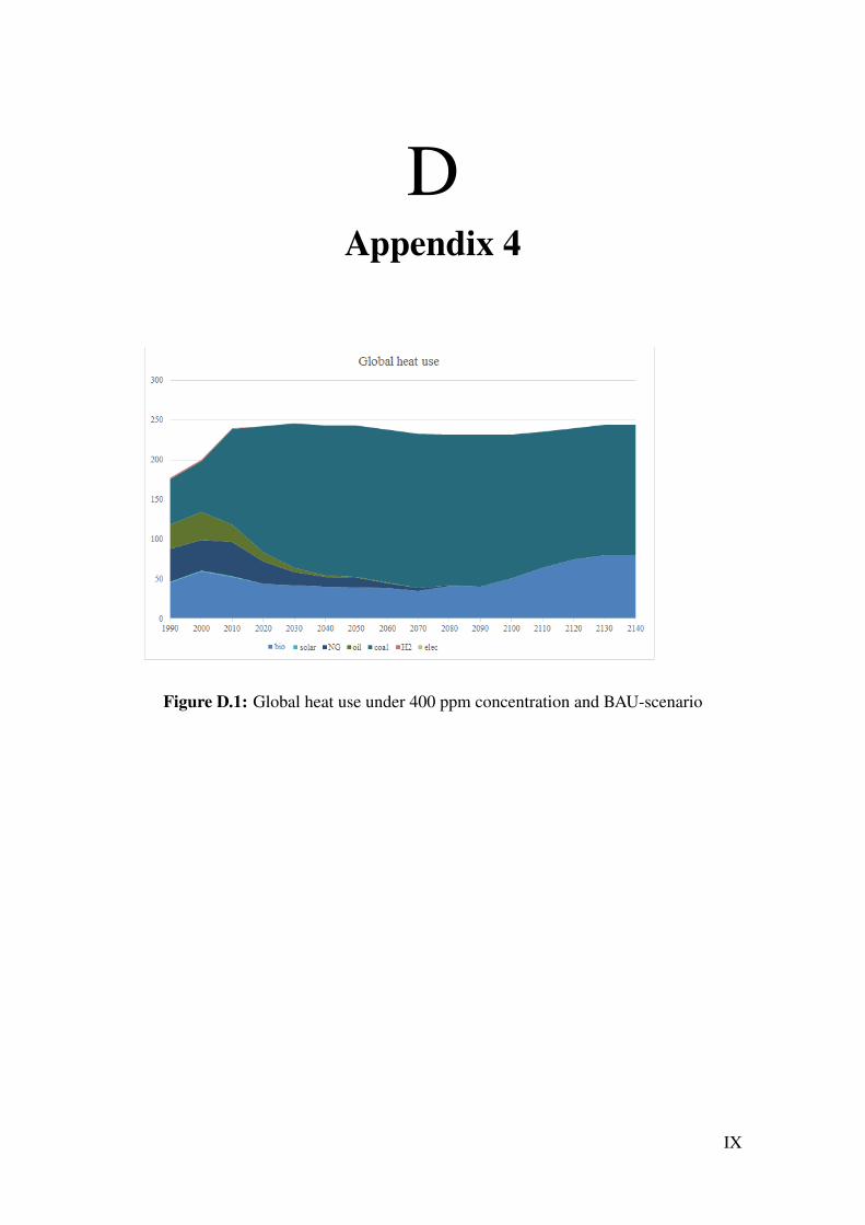
DAppendix 4

Figure D.1: Global heat use under 400 ppm concentration and BAU-scenario

IX

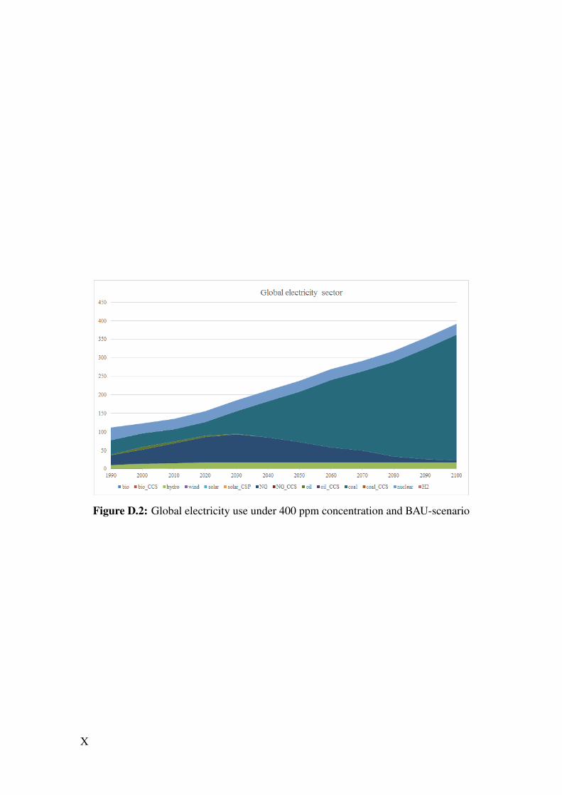
Figure D.2: Global electricity use under 400 ppm concentration and BAU-scenario

X