correction function for the lidar equation and some techniques for incoherent co_2 lidar data...

Correction function for the lidar equation and some techniquesfor incoherent CO2 lidar data reduction

Yanzeng Zhao, Ting Kaung Lea, and Richard M. Schotland

The convolution effect in CO2 lidar return signals caused by the long laser pulse is analyzed by modifying theoriginal lidar equation and introducing a correction function C,(R). The characteristics of C(R) arediscussed in detail, leading to a deconvolution technique consisting of a two-step iteration procedure for theextraction of both the backscattering coefficient and the gas species content in differential absorption lidarmeasurement.

1. Introduction

For lidar systems with long laser pulses, such as CO2lidar systems, extremely large signals, which are notexpected from the extrapolation of the far-range sig-nals, will be found in the near range. Based on thecommonly used lidar equation,

V(R) = CAE,37(R)7i2(R)/R2 , (1)

where V(R) = lidar return signal at range R,f3,(R) = atmospheric backscattering coefficient,T2 (R) = two-way transmittance, defined as

exp[- 2 jR (r)dr],

where is the atmospheric extinctioncoefficient,

E = energy of the laser pulse, andCA = system constant,

we have a linear equation derived from Eq. (1) in thehorizontal direction:

ln[V(R)R2 ] = ln(CA#,,) - 2,R. (2)

This is not true for CO2 lidar signals in the near range.A big hump will be superimposed on the straight linepredicted by Eq. (2), causing serious difficulties anderrors in extracting atmospheric parameters from thelidar signals.

Y. Zhao is with Cooperative Institute for Research in Environ-mental Sciences, Boulder, Colorado, 80309.

When this work was done all authors were with University ofArizona, Institute of Atmospheric Physics, Tucson, Arizona 85721;T. K. Lea is now at P.O. Box 1-3-24, Lung-tan, Taiwan 325, China.

Received 13 August 1987.0003-6935/88/132730-11$02.00/0.© 1988 Optical Society of America.

This puzzling phenomenon led the authors to goback to the original lidar equation to reexamine thevalidity of Eq. (1) in the case of long laser pulses and toestimate the severity of the cnvolution effect. Al-though the problem has been noticed by some re-searchers, such as Baker1 and Kavaya and Menzies,2 inmost cases it is neglected. Moreover, as far as weknow, no solution has been found. The situationstrongly suggests that a thorough discussion and anal-ysis are needed. It is the purpose of this paper to givemore insight into the problem and to describe sometechniques proposed for its solution. In Sec. II, amodified form of the original lidar equation is suggest-ed, and a correction function is introduced. Charac-teristics of the correction function C and the effect ofthe differences of C on DIAL measurement are dis-cussed in Secs. III and IV, respectively. The tech-niques used for extracting the atmospheric backscat-tering coefficient profile and the water vapor profileare given in Sec. V.

II. Modified Form of the Original Lidar Equation and theCorrection Function

Because of the finite length of the laser pulse, thelidar return signal at time t is the sum of the backscat-tered radiation by aerosols and molecules at differentranges along the propagation path in the atmosphere.Laser radiation emitted at t' and scattered back at thas reached the range

r = c(t - t')/2. (3)

For a given time t, the longest range corresponding tothe emitting time t' = 0 is r = ct/2. Hence the returnsignal V at time t is an integral from 0 to ct/2:

CO/2 P(t cr) * 7.2(r) * ,,(r) n(r)

Vi(t) = K r2 - dr, (4)

2730 APPLIED OPTICS / Vol. 27, No. 13 / 1 July 1988

where K = instrument constant,7(r) = receiving efficiency of the system,

P(t - 2r/c) = laser output power at time (t - 2r/c).Equation (4) is the original form of the single-scat-

tering lidar equation, which shows that the lidar returnsignal is a convolution of the laser output with othersystem parameters and atmospheric parameters.From Eq. (4), we have the energy-normalized lidarreturn signal:

VW ) Vi(t)E

ct/2 P(t _ 2r)* T2(r) fl(r) . n(r)E C r2KJ ~~~~ ~~~~dr. (5)

It is more convenient to use a range variable r for thelidar signal V and a time variable for the integral byintroducing the relations

2Rt'=t_ , R =ct/2,

from which we havect' ~cdt'r=R-2' dr=-

and consequently2RVC

V(R) = CAA

X[P(t')IE] TV(R ) * #_(R - Ct) r(R t

2 2 2 )2dt'

(R -ct')2

where CA = CK/2.Equation (6) is a version of the original lidar equa-

tion. The form of Eq. (6) indicates that it is difficult topredict the lidar return signal from Eq. (6) and tocompare Eq. (6) with Eq. (1). For purposes of compar-ison and further treatment, the authors suggest a mod-ified form for Eq. (6):

V(R) = CAfl,,(r)T 2 (r)Cr(R)/R2 . (7)

Equation (7) is very similar to Eq. (1), except for acorrection function Cr(R), which is defined as

1 2R/C / t \2Cr(R) = - P(t') 1- CC)

X ( 2 )1( 2 )XL L (R) ]

r( 2 )

ER P(t')S(R- 2 I) B(R- 2t)

X Tr(R- ') (R - c2)dt',

where

S(R - ct' -2 )( 2R)_

B( -t- [ ?(R -Q t')]

( C) r( ct')If laser pulse Xr is very short,

2)

and all the functions in the integrand in Eq. (8) will bevery close to unity; hence we have

i 2R/CC,(R) = E P(t')dt' 1.

Equation (7) reduces to Eq. (1), which is strictly validonly in the extreme case when the laser pulse is a deltafunction or reasonably accurate when the laser pulse isvery short. Since Eq. (1) is often referred to as thenormal lidar equation, the Cr(R) factor indicates adeparture from the normal lidar return signal.

Equation (7) provides a more useful form for theoriginal lidar equation 'because it is much easier tocompare the lidar signals of a long laser pulse withthose of a short pulse and to discuss the changing of thesignals by analyzing the features of the correctionfunction Cr. It is also easier to find a solution to theequation in certain circumstances.

The numerator on the right-hand side of Eq. (8) is aconvolution of laser power P(t') with the range-depen-dent functions S, B, Tr, and -q; hence Cr(R) is a ratio ofthe convolved functions to the energy of the laserpulse. Equation (8) also shows that Cr(R) is a normal-ized weighted range-dependent laser energy withweighting functions S, B, Tr, and -q. They modify thelaser pulse shape in the following way:

(1) As t' increases, the inverse range-square factor

S (R c)L~~~~~~~~~~ 2increases rapidly, thus strongly amplifying the effectof the tail of the laser pulse.

(2) Since the atmospheric transmittance always de-creases with range,

Tr (R ct)

increases with t' and also amplifies the laser tail.(3) If M3r(R) decreases with R, as usually happens in

the vertical direction,

B(R dt')

increases with t' and amplifies the laser tail; otherwise(8) it suppresses the tail.

(4) ij(R) increases rapidly with R and approaches

1 July 1988 / Vol. 27, No. 13 / APPLIED OPTICS 2731

unity within a few hundred meters for an incoherentlidar; hence

1(R- ct')

decreases with t' and more or less cancels the effect of

S (R -- c)' Tr (R - )

Because of the properties of the weighting functions,the tail of the laser makes a significant contribution tothe magnitude of Cr(R), even when the tail is 2-3 ordersof magnitude lower than the peak. The characteris-tics of C(R) related to laser pulse shape, receivingefficiency function, and atmospheric conditions arediscussed in detail in the next section.

111. Characteristics of Cr(R) for Incoherent CO 2 Lidar

Simulation calculations for a coaxial incoherent CO2lidar system have been carried out to illustrate thegeneral characteristics of Cr(R). The parameters ofthe lidar are listed in Table I. They are the same as theparameters for the CO2 lidar system at the Universityof Arizona. Since Cr(R) is the convolution of laseroutput with the atmospheric and system parameters,the length and shape of the CO2 laser are discussedfirst. The optical receiving efficiency are analyzednext. Finally, C(R) in the horizontal case and in thevertical case, in different atmospheric conditions, arediscussed in detail.

A. Pulse Shape of C02 Laser

It is well known that the output of a TEA CO2 laserstarts with a large spike (about tens of nanoseconds)followed by a long tail of several microseconds. Al-though the magnitude of the tail far away from thespike is several decades lower than that of the spikeand is often neglected, it still has significant contribu-tions to Cr(R) up to 2-3 km, as shown in our calcula-tions. It is, therefore, crucial to have detailed knowl-edge of the pulse shape, particularly that of the tail.Unfortunately, the accurate measurement of the pulseshape throughout its whole length is extremely diffi-cult, if not impossible, because the requirements of thelarge dynamic range (5-6 decades), wide bandwidth,and sufficient SNR can hardly be met at the same time.However, it is feasible to obtain a fairly good quantita-tive picture of the laser pulse by simulation calcula-tion. As Duley3 pointed out, the accuracy of modeling

Table 1. Main Parameters of the Ldar System used In the Computation

Parameters of the laserGas mixing ratios

Long pulse He:CO 2:N2 = 9:1:0.7Short pulse He:CO 2:N 2 = 6.2:1:0

Beam divergence 2 mrad

Parameters of the receiverDiameterof the primary mirror 44.5 cmFocal length of the primary mirror 203.8 cmField of view 6 mradDiameter of the central obscuring screen 10 cm

Fig. 1. Schematic diagram of the energy level related to CO2 laser.

calculation is "now at the stage where output powershapes from TEA lasers can be predicted with littledeviation for measured pulse shape." The modelingcalculations of Manes and Seguin4 and Andrews et al.

5

show a good agreement between the theoretical andexperimental results in a range where the laser powercan be measured. We expect that reasonable timevariation of the tail will also be obtained by theoreticalcalculation.

In our calculation, the simplified model of Andrewset al. is modified by adding an electron excitation termand a deexcitation term to each equation for lowerlevels of C02. Following the same nomenclature, theschematic of the energy level related to a CO2 laser isillustrated in Fig, 1, and the rate equations are given asfollows:

dnl/dt = al(no - fn1 ) - K13nl

+ (Nno - nN 0) - sq(n -n2)

dn2/dt = 2(no - fn 2) - K2n2 + sq(n -n2)

dn3/dt = a3(no - fn 3 ) + K2n2 K3n31

dN/dt = (No - fN) - K(Nno -njN)

dqldt = sq(n - n2) - wq + Dnj, (9)

where ni, n2, n3, and no are the population densities ofC02 at (001), (100), (010), and ground level, respective-ly; N and NO are the population density of N2 at v = 1and ground level, respectively; al and 3 are proportion-al to the electron density in the discharge, K13, K2, K3,

and K are the relaxation rates for (001), (100), (010)levels of C02 and v = 1 level of N2 , respectively; q is thephoton density; s is the simulated emission rate; w isthe cavity loss rate; and D is the spontaneous emissionrate.

By applying all the parameters of the C02 laser(Lumonics 103-2) used in our lidar system, we calcu-late the time variations of the output power, inversionpopulation density, and gain coefficient for two specif-ic mixing ratios of He, C02, and N2 . He:CO 2 :N2 =9:1:0.7 for the long pulse was suggested by the manu-facturer. He:CO2 :N2 = 6.2:1:0 for the short pulse wasthe optimized one found in or experiments. Thecalculated pulse energies are in good agreement withour experiments, although the accurate pulse shapehas not yet been measured, due to the time responseand the dynamic range of the detectors.

Energy normalized laser power PIE plotted on thelog scale and linear scale as a function of time fordifferent gas mixing ratios is shown in Figs. 2; theaccumulated output energy as a function of time isshown in Fig. 3. The general characteristics of the


6

& 5

5

So2I --

4.5aE6

4.00E6

3 3.50E6

a)2.56

2.aE06

- .50E6

E 1.E06

5.0065

0.0060

Z

E

time (m cro.econ -)

(cl

.20E7

.0E7

6.006

4.00E6

2.006

0.0060

3cI

IS

.2

I

E

Io

(bI

time (mi r - ,0d I

(dl

t icrosecon.. .ime {in re.on d

Fig.2. Normalized laser pulse shape P(t)/E: (a) long pulse: He:CO2 :N2 = 9:1:0.7 (log scale); (b) short pulse: He:C0 2 :N2 = 6.2:1:0 (log scale);

(c) long pulse as (a) (linear scale); (d) short pulse as (b) (linear scale).

laser pulse are clearly seen in the figures. The mostimportant and interesting results related to the convo-lution effect are as follows:

(a) The long pulse tail always exists, even whenthere is no N2 . After N2 is removed, the tail is hardlyseen in a linear system, but it is still obvious in a log-scale plot and lasts for several microseconds. Al-though, in the case without N2, the tail contains muchless energy, its contribution to Cr(R) is still significant.

(b) The tail of the pulse does not drop down expo-nentially but decreases much faster. It implies that ifa simple exponential model is used in Eq. (8), theconvolution effect might be exaggerated.

B. Near-Range Signal-Receiving Efficiency Function

As discussed in Sec. II, an opposite factor whichlimits the enlargement effect of the inverse rangesquare is the near-range signal-receiving efficiencyfunction. For a biaxial lidar system, the signal-receiv-ing efficiency is none other than the overlapping func-tion. For a coaxial lidar system, the signal-receivingefficiency depends mainly on two effects: the defocus-ing effect (if the focal length of the primary mirror ofthe receiver is not negligible compared to the range)and the central obscuring effect. The former causes abeam size at the focal plane greater than the field stopof the detector. The latter is a consequence of themasking effect of the diagonal reflector, which makesthe transmitting laser beam coaxial with the receiver.The shadow of the diagonal reflector at the focal planefalls within or intersects with the field stop, resultingin a reduction of the signal.

For a biaxial system, the overlapping function 7(R)is usually zero or near zero within several hundred

1 2 3

TIME (II CROSECONO I

Fig. 3. Integrated laser energy as a function of t:short pulse.

1, long pulse; 2,

meters, thus considerably canceling the effect of thetail and consequently reducing the magnitude ofCr(R). However, for a coaxial system, the bline zone isonly a few meters, and 77(R) quickly approaches unitywithin a hundred meters. The canceling effect is,therefore, substantially restricted. In the followingsection, n1(R) is mainly calculated for the system pa-rameters in Table I. The intensity distribution of thelaser beam within 100 m assumes the following pat-tern:

I(r) = Io exp[-(r - 0.6r0 )2/0.lro], (10)

where ro is the radius of the beam, and r is the radialdistance from the center of the beam. The resultant7(R) is plotted as curve 1 in Fig. 4 with the centralscreen diameter DC = 10 cm.


0o

0.80 _

=0.730

0.60 /

0.50

. 0.40

0.0 I

0.20

0.1 -

0.00

0 60 (20 10 240 300 0 360 420 540 600

range (m

Fig. 4. Receiving efficiency functions: 1, coaxial system; 2, biaxialsystem.

1(R) for a biaxial system with a 40-cm separation ofthe axes, 2-mrad divergence for transmitting beam and2.5 mrad for field of view is calculated and shown inFig. 4 as curve 2. The intensity distribution of thebeam is assumed to be Gaussian.

C. CAR) in the Horizontal Case

The horizontal case is the simplest one, where thebackscattering and extinction coefficient are approxi-mately constant; therefore, the effect of pulse lengthcan be seen more clearly. In the horizontal case,

Tr (R ct =exp[ o(R - )]. = exp(caot').exp(-2a0R)

B (R c) =1.

Hence1 2R/C ( ct cto)

Cr(R)= PWt)S (R - i-c'>) (R~ - exp(ccrot')dt'. (11)

The transmittance factor in the integrand takes thepositive exponential form exp(ccot'); thus its role ofamplification of the pulse tail and the relation of theamplification to the extinction coefficient o, as dis-cussed earlier, are more explicit.

The correction functions are calculated for CO2 laserpulses with the specific parameters given in Sec. III.A.The results for both coaxial and biaxial lidar configu-rations are shown in Figs. 5 and 6. One of the moststriking features of Cr(R) is that there is always a bighump in the near range, whether or not there is nitro-gen in the laser gas mixture. For a long laser pulsewith nitrogen in the cavity, the peak of the hump is 3.5for a weak absorption case ( = 0.2 km-), increasingto 7.2 for a higher absorption case (o = 1.5 km-'). Itmeans that the departure of the lidar signal from thenormal lidar return can be as high as 250-620%.Hence the puzzling hump found in our early observa-tion is partly explained by the convolution effect of thelong laser pulse. (The remaining part is attributed tothe scattering of the steering mirror when the system isnot properly aligned.)

It is also interesting to note that even for the shorterCO2 laser pulse, when nitrogen is removed, the peak of

0 600 1200 1800 2400

Hrzont l rge (ml

Fig. 5. Correction function in the horizontal case for a long pulse:la, extinction coefficient = 0.2/km, coaxial system; lb, extinctioncoefficient = 1.5/km, coaxial system; 2a, extinction coefficient = 0.2/km, biaxial system, axes separation = 40 cm; 2b, extinction coeffi-

cient = 1.5/km, biaxial system, axes separation = 40 cm.

. 2.0

= . 5I.,

t I .5u

0.5

0.0

0 600 1200 1800 2400

Horizontal Rn-ge R (.l

Fig. 6. Correction function in the horizontal case for a short pulse:la, extinction coefficient = 0.2/km, coaxial system; lb, extinctioncoefficient = 1.5/km, coaxial system; 2a, extinction coefficient = 0.2/km, biaxial system, axes separation = 40 cm; 2b, extinction coeffi-

cient = 1.5/km, biaxial system, axes separation = 40 cm.

Cr(R) is still very large: 1.9 for c = 0.2 km- 1 and 2.5for 0o = 1.5 km-'. The unseen long tail of the pulse inthis case shows its significant contribution of thehump, as mentioned in Sec. III.A. It implies that theconvolution effect cannot be circumvented by simplyremoving nitrogen from the gas mixture.

For a more general analysis dealing with the effect ofthe pulse shape on the characteristics of the hump, aparametrized laser pulse shape is also used. It as-sumes the following form:

P(t) = exp[A(0.25t2/tl2) exp(- t + 2) + B - Ct3]

t < 15t,; (12)

P(t) = exp[B - G(t - 15tj) - H(t - 15t1)2 - Ct3

t > 15t1 .

Five sets of parameters have been chosen for thelaser pulse, and the normalized shapes are shown in


34

s in

I .00

0.90

0.a0

0.70

0.5

0.0*

0.640 25i .0 -

.0 --

0.320-

0. 5-0.) 0

0.00 0.0

0 0.05 0.1 0 0.9 0.20 0.25 0.30 0 300

time (ic~rosecon d

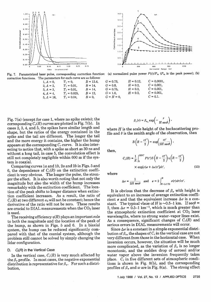
Fig. 7. Parametrized laser pulse, corresponding correction function: (a) normalized pulse power

correction functions. The parameters for each curve are as follows:1,A = 0, T = 0, B = 13.4, G = 0.73, H= 0.12,2,A = 2, T, = 0.01, B = 14, G = 0.8, H= 0.2,

3, A = 3, T = 0.01, B = 14, G = 0.75, H = 0.3,4, A = 4, T = 0.025, B = 12, G = 1.0, H = 0.2,5,A=16, T1=0.04, B=0, G=H=0,

Fig. 7(a) (except for case 1, where no spike exists); thecorresponding Cr(R) curves are plotted in Fig. 7(b). Incases 2, 3, 4, and 5, the spikes have similar length andshape, but the ratios of the energy contained in thespike and the tail are different. The longer the tailand the more energy it contains, the higher the humpappears at the corresponding Cr curve. It is also inter-esting to notice that, with a spike as short as 30 ns andwithout a long tail, in case 5, the convolution effect isstill not completely negligible within 600 m if the sys-tem is coaxial.

Comparing curves la and lb, 2a and 2b in Figs. 5 and6, the dependence of Cr(R) on the extinction coeffi-cient is very obvious. The longer the pulse, the stron-ger the effect. It is also worth noting that not only themagnitude but also the width of the hump increasesremarkably with the extinction coefficient. The loca-tion of the peak shifts to longer distance when extinc-tion coefficient increases. As a result, the ratio ofCr(R) at two different co will not be constant; hence thederivative of the ratio will not be zero. These resultsare crucial to DIAL measurements when the CO2 laseris used.

The receiving efficiency 7(R) plays an important roleto both the magnitude and the location of the peak ofthe hump, as shown in Figs. 5 and 6. In a biaxialsystem, the hump can be reduced significantly com-pared with that of the coaxial system, although theproblem still cannot be solved by simply changing thelidar configuration.

D. CAR) in the Vertical Case

In the vertical case, Cr(R) is very much affected bythe Fl, profile. In most cases, the negative exponentialdistribution is representative for F,. For such a distri-bution,

600 900 1200

Horizonal Rango ()

P(t)/Pm (Pm is the peak power); (b)

C = 0.0001,C = 0.001,C = 0.001,C = 0.001,C=0.1.

/7(r) = :,~ exp( H secO)

where H is the scale height of the backscattering pro-file and 0 is the zenith angle of the observation, then

B (R - ) = exp( ct')

then,

C()=E A P(t')S (I- 2 ) o(-2)

X exp[c(o + A-)t'Idt', (13)

whereR

a= 1 and a = 2 o(r)dr/ct'.2H secO JR-(ct'/2)

It is obvious that the decrease of A3r with height isequivalent to an increase of average extinction coeffi-cient a and that the equivalent increase Au is a con-stant. The typical vlaue of H is -0.5-1 km. If secO =2, then Au = 0.5-1 km- 1 , which is much greater thanthe atmospheric extinction coefficient at CO2 laserwavelengths, where no strong water-vapor lines exist.As a consequence, significant changes of Cr(R) andserious errors in DIAL measurements will occur.

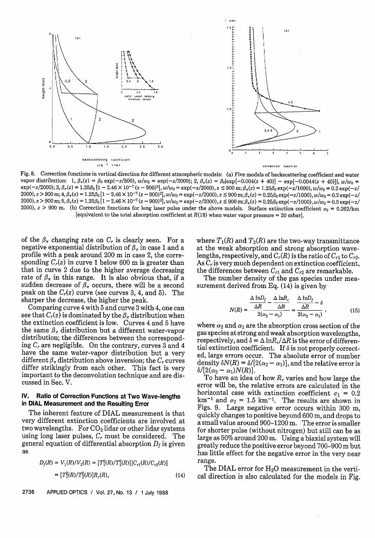
Since Au is a constant in a simple exponential distri-bution of pr the shapes of Cr in the vertical case are notvery different from those in the horizontal case. Wheninversion occurs, however, the situation will be muchmore complicated, as the variation of fir is no longermonotonic, and the sudden drop of aerosol and/orwater vapor above the inversion frequently takesplace. Cr in five different sets of atmospheric condi-tions is shown in Fig. 8(b), and the correspondingprofiles of f0, and w are in Fig. 8(a). The strong effect


4. 0

4.5

0.0 0.5 1.0 t.5 2.0 2.5 3.00'0 1 2 0 4 5 6 7

b.,ck-tatering aeffi-ten

(In) 6 Im orrectlion Runction

Fig. 8. Correction functions in vertical direction for different atmospheric models: (a) Five models of backscattering coefficient and watervapor distribution: 1, fl,(z) = o exp(-z/500), w/wo = exp(-z/2000); 2, (z) = flolexp[-0.004(z + 40)] - exp[-0.0044(z + 40)]I, w/wo =exp(-z/2000); 3, 0,3(z) = 1.25flo [1 - 2.46 X 10-7 ( - 900)2], w/wO = exp(-z/2000), z • 900 m; A,,(z) = 1.25o exp(-z/1000), w/wo = 0.2 exp(-z/2000), z > 900 m; 4, :,(z) = 1.2500 [1 -2.46 X 10-7 ( - 900)2], w/wo = exp(-z/2000), z < 900 m; f3,,(z) = 0.25flo exp(-z/1000), w/wo = 0.2 exp(-z/2000), z > 900 m; 5, ,(z) = 1.2 5fo [1 -2.46 X 10-7 (Z - 900)2], W/wo = exp(-z/2000), z S 900 m; 3,(z) = 0.25flo exp(-z/1000), w/wo = 0.5 exp(-z/2000), z > 900 m. (b) Correction functions for long laser pulse under the above models. Surface extinction coefficient a = 0.262/km

[equivalent to the total absorption coefficient at R(18) when water vapor pressure = 20 mbar].

of the 0, changing rate on C is clearly seen. For anegative exponential distribution of 37, in case 1 and aprofile with a peak around 200 m in case 2, the corre-sponding Cr(z) in curve 1 below 600 m is greater thanthat in curve 2 due to the higher average decreasingrate of 37, in this range. It is also obvious that, if asudden decrease of 0, occurs, there will be a secondpeak on the Cr(z) curve (see curves 3, 4, and 5). Thesharper the decrease, the higher the peak.

Comparing curve 4 with 5 and curve 3 with 4, one cansee that Cr(z) is dominated by the , distribution whenthe extinction coefficient is low. Curves 4 and 5 havethe same /, distribution but a different water-vapordistribution; the differences between the correspond-ing Cr are negligible. On the contrary, curves 3 and 4have the same water-vapor distribution but a verydifferent /37, distribution above inversion; the Cr curvesdiffer strikingly from each other. This fact is veryimportant to the deconvolution technique and are dis-cussed in Sec. V.

IV. Ratio of Correction Functions at Two Wave-lengthsin DIAL Measurement and the Resulting Error

The inherent feature of DIAL measurement is thatvery different extinction coefficients are involved attwo wavelengths. For CO2 lidar or other lidar systemsusing long laser pulses, C must be considered. Thegeneral equation of differential absorption Df is givenas

Df(R) = V(R)/V 2 (R) = [(R)/TV(R)][Cri(R)/Cr 2 (R)]

= [(R)/T7(R)]R,(R), (14)

where T1(R) and T 2(R) are the two-way transmittanceat the weak absorption and strong absorption wave-lengths, respectively, and Cr(R) is the ratio of Cr1 to Cr2.As Cr is very much dependent on extinction coefficient,the differences between Cri and Cr2 are remarkable.

The number density of the gas species under mea-surement derived from Eq. (14) is given by

A lnDf A InR An aAR AR ARN(R) = (15)

2(a2 - a 2 (cr2 - a)

where a and al are the absorption cross section of thegas species at strong and weak absorption wavelengths,respectively, and 6 = A lnR,/AR is the error of differen-tial extinction coefficient. If b-is not properly correct-ed, large errors occur. The absolute error of numberdensity AN(R) = 6/[2(a2 - a)], and the relative error is6/[2(a2 - al)N(R)].

To have an idea of how R, varies and how large theerror will be, the relative errors are calculated in thehorizontal case with extinction coefficient o-l = 0.2km-' and a.2 = 1.5 km-'. The results are shown inFigs. 9. Large negative error occurs within 300 m,quickly changes to positive beyond 600 m, and drops toa small value around 900-1200 m. The error is smallerfor shorter pulse (without nitrogen) but still can be aslarge as 50% around 200 m. Using a biaxial system willgreatly reduce the positive error beyond 700-900 m buthas little effect for the negative error in 'the very nearrange.

The DIAL error for H20 measurement in the verti-cal direction is also calculated for the models in Fig.


I1 t a-

60 -

o.0

I . /

* 3_;2 .

1 Id

0 1 2

h.riznta rnge (ki)

2 0 -IR b

I 9

a -i *1 ) 0XO- I ..

0I ,d s.__*

0'--

- I 0 -

-20 -

- 0 -

-40 -

-5 0 -

Z k)

.0_

2.0_

1.0 _

O _

horiznta rIngn (ki)

Fig. 9. Relative errors in the DIAL measurement in the horizontalcase. Atmospheric extinction coefficient at off-line and on-linewavelengths are a, = 0.2/km, a2 = 1.5 km: (a) for long pulse: 1,coaxial system; 2, biaxial system, axes separation = 40 cm; 3, biaxialsystem, axes separation = 60 cm; (b) for short pulse: 1, coaxialsystem; 2, biaxial system, axes separation = 40 cm; 3, biaxial system,

axes separation = 60 cm.

-60

2 (kin

. 0 r

2.0

0 L..0.0 0.4 0.5 0.6 0.7 0.8 0.9

Rc

Fig. 10. Ratios of the correction function at R(18) to that at R(20)for the atmospheric models in Fig. 8(a). Surface water vapor pres-

sure = 20 mbar.

-40 -20

(b)

0 20 40 60 80 1 00 20

,t i rror . )

Fig. 11. Relative errors in DIAL measurement for water vapor inthe vertical direction under the atmospheric models in Fig. 8(a): (a)

for long pulse; (b) for short pulse.

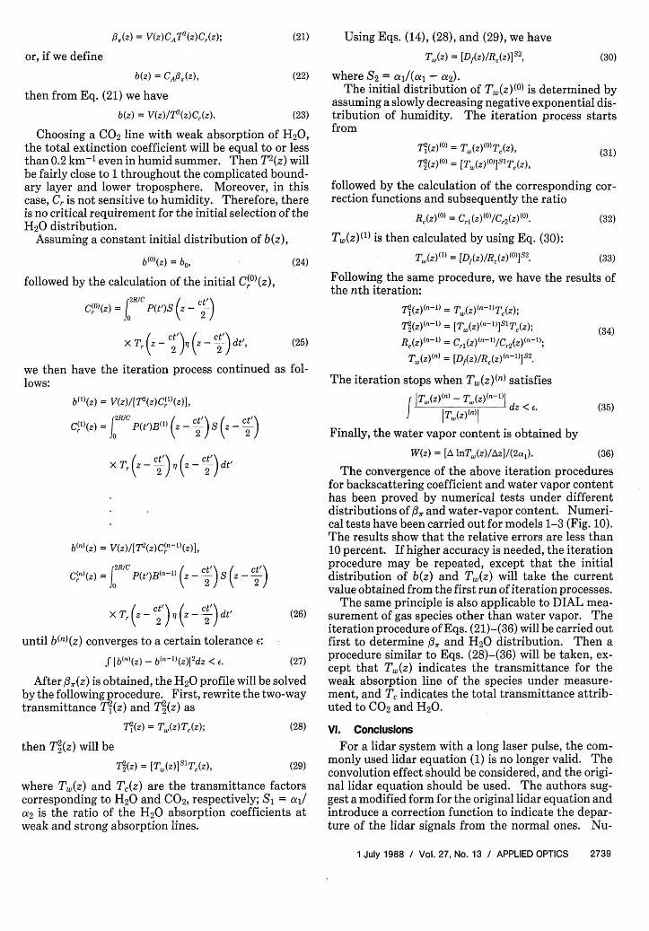
8(a). H20 lines R(18) and R(20) are chosen for thiscalculation, and the absorption cross sections are tak-en from Shumate et al.6 CO2 absorption is also includ-ed. R, for the five models is shown in Fig. 10. Relativeerrors are plotted against height in Figs. 11. Thegeneral features of the errors as a function of height aresimilar to those in horizontal cases, except in the regionjust above the inversion height, where deep dropdownof H20 takes place, causing extremely large relativeerrors.

If just the sensitivity of 6 to the backscattering pro-file and water vapor profile is considered, very inter-esting things are found. In Fig. 12(a), one can see that,in spite of very different /, distributions, the 3 valuesfor models 1, 2, and 3 are quite close to each otherbelow 900 m, where the H20 distributions are thesame. Above 900 m, the 6 for model 3 drops down veryfast because water vapor decreases much faster than in


40 -

20 -

Ro

IaIa

2I

20 -

40 -

60 a

nreliu (%

To l A*^^n |

11I Iq

II I01 . �k

I:I. I

[

2I 0

2

I.00

I

I

.2

2I

Ti(t',z) and T 2(t',z) between 0 and 2z/c with theweighting function g(z,t'). From Eq. (17), we have

[ T'2 (z) 1L .(1(a) )= Az_ . . (18)

While ln(lTr/Tr2) is proportional to column water-va-por content

J N(z)dz,

and its derivative is proportional to N(z), n[Tia(z)/TVa(Z)] is not the case; we can write 6 as

a = f(z)N(z). (19)

If f(z) does not change very much in two cases, a and b,where g(t',z) remains the same, then

n

(. 0 -Ž0

.0:

IbI

t~b(~O mb

0 . . 'I...I.......-2.5 -2.0 -(.5 -I.0 -0.5 0. 0.5 (.0 (.5 2.0

Fig. 12. Sensitivity of A nR,/Az to the backscattering coefficientdistribution and the water vapor content: (a) A lnR/Az for models1, 2, and 3 in Fig. 8(a); surface water vapor pressure = 20 mbar; (b) A

lnR,/Az for model 1 under two surface water vapor pressures.

the other two models. On the contrary, the 6 calculat-ed for model 1, with two different values of surfacewater vapor pressure, i.e., 20 and 10 mbar, show sub-stantial differences [see Fig. 12(b)]. The ratio of thetwo 6 distributions is almost equal to the ratio of thewater vapor. As a matter of fact, if we define

g(t',z) = P(t')S(t',z)B(t',z)o(t',z), (16)

the ratio2R/C

C, (Z) lo g(t',z)7 I (t',z)dt' T2 (z)R C r2 Z - -- -- (17)

w h e r e T Oa( Z ) a n dg (t a z ) t ( t z) d t e a v r g o f

where 7l1,(z) and 72,,(z) are the weighted averages of

(20)

From Eqs. (17)-(19), it is easy to understand thatbecause 37, is included in both the numerator and de-nominator in the expression of R,, 6 is not sensitive to/, distribution. For the same reason, it is also expect-ed that 6 is not sensitive to changing the laser pulseshape, provided that pulse lengths at the two wave-lengths are approximately the same.

V. Deconvolution Technique for Incoherent CO2 LidarMeasurement

The above sections have shown a quite complicatedpicture of CO2 lidar return signals and the difficultiesof data reduction. There is no simple way to overcomethe difficulties. As long as the pulse tail lasts forseveral microseconds, one has to face the problem ofdeconvolution, if the near-range information of thelower atmosphere is desired.

Three facts are crucial to the deconvolution tech-nique:

(a) The aerosol extinction coefficient at 10 gtm isvery small, almost negligible, compared with the totalabsorption coefficient of CO2 and H2 0; therefore, thebackscattering and transmittance factors in the lidarequation in clear atmosphere conditions are essential-ly independent of each other.

(b) The correction function Cr is very sensitive to /37r

distribution but insensitive to the water-vapor amountand distribution at wavelengths with weak absorptionof H2 0.

(c) The ratio of correction functions at two wave-lengths in DIAL measurement of H20 is insensitive tothe /, distribution and very sensitive to the H20amount and distribution.

Based on the above facts, a two-step iteration proce-dure is proposed, in which /, profile and H20 profilecan be extracted separately from the lidar equation.

The /, profile is the first to be extracted. From lidarEq. (7), we have


I (k-n

0.0

,.0

0.5 1.0 1.5 2.0

ba/bb WWb-

0,,(Z) = V(Z)CAT(Z)Cr(Z);

or, if we define

(21) Using Eqs. (14), (28), and (29), we have

T"(z) = [Df(Z)/Rc(z)]S2,

b(z) = CA/3r(Z), (22)

then from Eq. (21) we have

b(z) = V(z)/T 2 (z)Cr(z). (23)

Choosing a C02 line with weak absorption of H2 0,the total extinction coefficient will be equal to or lessthan 0.2 km-1 even in humid summer. Then T2 (z) willbe fairly close to 1 throughout the complicated bound-ary layer and lower troposphere. Moreover, in thiscase, Cr is not sensitive to humidity. Therefore, thereis no critical requirement for the initial selection of theH20 distribution.

Assuming a constant initial distribution of b(z),

b(°)(z) = b,

followed by the calculation of the initial C(°)(z),

C(0)(Z) = P(t')S (ZCt

X Tr (Z-C2 )- (Z- 2 )

we thenlows:

(24)

where S2 = a,/(a 1 - a2)-The initial distribution of T(z)( 0 ) is determined by

assuming a slowly decreasing negative exponential dis-tribution of humidity. The iteration process startsfrom

(31)7'( W() = T (Z)(0)T (z),

712W (0) = [T.(Z)(o)]slTc(z),

followed by the calculation of the corresponding cor-rection functions and subsequently the ratio

(32)R,(z)( 0) = C,1(Z)(°)/C2 (Z)(°).

T.(Z)(1) is then calculated by using Eq. (30):T (z)()= [Df(z)/R,(z)(0)]S2. (33)

Following the same procedure, we have the results ofthe nth iteration:

(25)

have the iteration process continued as fol-

b0)(z) = V(z)[7(z)C(')(z)1,

C1)'(z) = j P(t')B(I) (z ct)S( _ CtI)

X Tr -_ Q) o7 (z - ct)dt'( 2 )( 2

b(n)(Z) = V(Z)1[V1(Z)C~n-l)(Z)],

C~n)(Z) = j P(tn)B~n-1) ( _ ( _ Ct1)

. Tr (S-- )Z C t')

until b(n)(z) converges to a certain tolerance E:

f I bn(z) - b(n-1)(z) 2dz < . (27)

After / , (z) is obtained, the H20 profile will be solvedby the following procedure. First, rewrite the two-waytransmittance T 2(z) and T2(z) as

71(z) = T(z)T,(z); (28)

then T2(z) will be

T2(z) = [T,(z)]S 1 Tc(z), (29)

where T(z) and T,(z) are the transmittance factorscorresponding to H20 and C02, respectively; SI = ai/a2 is the ratio of the H20 absorption coefficients atweak and strong absorption lines.

,(Z)(n-l) = T (Z)(n-1)Tj~Z);

r2(Z)(n-1) = [Tw(Z)(n-1)]SlTc(z);

Rc (Z)(n-1) = Crl(Z) (n-')/C,2(Z) (n-1);

T,(Z)(n) = [Df(z)/R,(z)(n-l)]s2.

The iteration stops when T(z)(n) satisfies

I |T.W(n)- T.(z)(n-1)

J IT. (z(n)l d < .

Finally, the water vapor content is obtained by

W(z) = [A lnT.(z)/Az]/(2aj).

(34)

(35)

(36)

The convergence of the above iteration proceduresfor backscattering coefficient and water vapor contenthas been proved by numerical tests under differentdistributions of , and water-vapor content. Numeri-cal tests have been carried out for models 1-3 (Fig. 10).The results show that the relative errors are less than10 percent. If higher accuracy is needed, the iterationprocedure may be repeated, except that the initialdistribution of b(z) and T(z) will take the currentvalue obtained from the first run of iteration processes.

The same principle is also applicable to DIAL mea-surement of gas species other than water vapor. Theiteration procedure of Eqs. (21)-(36) will be carried outfirst to determine , and H20 distribution. Then aprocedure similar to Eqs. (28)-(36) will be taken, ex-cept that T(z) indicates the transmittance for theweak absorption line of the species under measure-ment, and T, indicates the total transmittance attrib-uted to C02 and H20.

VI. Conclusions

For a lidar system with a long laser pulse, the com-monly used lidar equation (1) is no longer valid. Theconvolution effect should be considered, and the origi-nal lidar equation should be used. The authors sug-gest a modified form for the original lidar equation andintroduce a correction function to indicate the depar-ture of the lidar signals from the normal ones. Nu-


(30)

merical simulation shows that the general features ofthe Cr(R) are as follows:

(a) In most cases and for most of the ranges con-cerned, C > 1, and there is always a hump in the nearrange. The peak of the hump can be as large as 3.5 inthe horizontal direction for a typical incoherent CO2lidar in long-pulse operation at weak absorptionlengths.

(b) C(R) depends on laser pulse shape, particularlythe length and form of the tail. C(R) also depends onthe configuration of the lidar.

(c) C(R) is sensitive to atmospheric transmittanceand is very different for the on-line and off-line wave-lengths, causing large errors in DIAL measurements ifit is not considered.

(d) C(R) is sensitive to backscattering distribution.In the case of CO2 lidar, since the backscattering

coefficient and the extinction coefficient are essential-ly independent of each other, and since the extinctioncoefficients at off-line wavelengths are very small andhave a negligible effect on Cr(R), a two-step iterationprocedure is proposed for the deconvolution of thelidar return signal for the extraction of both the back-scattering coefficient and the gas species content inDIAL measurement. The convergence of the proce-dure has been proven by numerical tests.

The authors wish to thank D. Winker for his help incomputer programming and A. Hugo for the helpfuldiscussions. Special thanks are owed to M. Sander-son-Rae for her efforts in editing the original manu-script of this paper.

Yanzeng Zhao is on leave from the Institute of Atmo-spheric Physics of the Chinese Academy of Sciences.

References

1. P. W. Baker, "Atmospheric Water Vapor Differential AbsorptionMeasurements on Vertical Paths with a CO2 Lidar," Appl. Opt.22, 2257 (1983).

2. M. J. Kavaya and R. T. Menzies, "Data Acquisition, Data Pro-cessing, Parameter Modeling, and Hard Target Calibration forAccurate Lidar Aerosol Backscatter Measurements," in Ab-stracts of Papers, Twelfth ILRC (Aix en Provence, France, Aug.1984).

3. W. W. Duley, C0 2 Lasers: Effects and Applications (Academic,New York, 1976).

4. K. R. Manes and H. J. Seguin, "Analysis of the CO2 TEA Laser,"J. Appl. Phys. 43, 5073 (1972).

5. K. J. Andrews, P. E. Dyer, and D. J. James, "A Rate EquationModel for the Design of TEA CO2 Oscillators," J. Phys. E 8, 493(1975).

6. M. S. Shumate, R. T. Menzies, J. S. Margolis, and L.-G. Rosen-gren, "Water Vapor Absorption of Carbon Dioxide Laser Radia-tion," Appl. Opt. 15, 2480 (1976).

FIBER STRENGTH TERMS

Strength * The fracture stress over a unit area for aparticular set of loading conditions.

Proof Test * Applying constant stress to an entirelength of fiber to guarantee minimum strength.

Weibull Plot * A statistical graph used to show dataplotted as cumulative failure probability versus aload, stress or time at failure.

Fatigue * Reduction of fiber strength over time.

'n" * A measure of the glass material's susceptibil-ity to fatigue, sometimes referred to as the stress-corrosion susceptibility factor.

Strain Rate * The rate at which stress is applied toincrease strain on a fiber during a tensile test.

Gauge Length * Measured length of fiber undertest.

Copies o this material may be distributed withappropriate credit to Corning Glass Works

CORNING


correction function for the lidar equation and some techniques for incoherent co_2 lidar data...

Documents