1

Corporate Cash Holdings and Monetary Shocks

Yiling Deng1 and Haibo Yao

2

Abstract

This paper examines the impact of monetary shocks on corporate cash holdings.

We find evidence that small industrial firms hold onto cash when monetary policy is too

tight and large industrial firms do the reverse both in the short-run and in the long-run.

Further tests examine whether the long lasting loose monetary policy results in the pileup

of corporate cash holdings. The evidence supports the assumption that industrial firms

take the “long lasting lower interest rate” environment to hoard cash to buffer the

monetary policy effectiveness.

Key words: Cash Holdings; Monetary Shocks; Taylor Rule

JEL: G30, G32, E30, E43, E52

1 Robinson Collage of Business School, Georgia State University, Email: ydeng5@gsu.edu

2 Walker L. Cisler College of Business, Northern Michigan University, Email: hyao@nmu.edu

2

Industrial firms hold cash for many reasons. John Maynard Keynes (1936) posits

three motives: a transaction motive, a precautionary motive, and a speculative motive.

The transaction motive for money demand results from the need for liquidity for day-to-

day transactions to bridge the gap between payments and receipts. The precautionary

demand for money refers to holding cash to minimize the potential loss arising from a

contingency when access to capital markets is costly. Speculative demand for cash refers

to holding cash to take advantage of investment opportunities that may arise in the future.

Bates et al. (2009) find evidence supporting both the transaction motive and the

precautionary motive from firm specific explanations. They also report consistent

evidence supporting an increase in cash holdings in the 2000s that cannot be explained by

changes in firm characteristics.

“One way of understanding why U.S. firms have amassed so much cash is to

recognize that holding cash provides firms with unexercised option value, giving them

financial flexibility in times of heightened uncertainty.”3 Hodrick (2013) cites the

example of Google’s CFO Patrick Pichette’s motivating the company’s holding $48.1

billion of cash at the end of 2012 as giving it “the strategic ability to pounce.”4 Another

example is that “Warren Buffet is noted to think of cash held in his portfolio as a call

option allowing him to obtain cheap assets at fire sale prices (such as his $5 billion

investment in Goldman Sachs in the depths of the financial crisis).”5 Industrial firms

choose their optimal cash holdings in response to market challenges including uncertain

economic, fiscal, and monetary environment such as the sustainability of historically low

3 “Are U.S. Firms Really Holding Too Much Cash?” by Laurie Simon Hodrick, Stanford Institute for

Economic Policy Research (SIEPR) policy brief, July, 2013. 4 Morgan Stanley Technology Conference, February 29, 2013.

3

interest rates. These uncertainties create corporate cash flow volatility, resulting in the

option value of holding cash.

As far as we know, however, none of the prior empirical corporate cash holdings

studies define and use monetary policy shocks (or tightening). As measures of monetary

tightening, nominal interest rates and changes in nominal rates could prove misleading

and could induce perverse results6 (Fisher, 1930; Friedman, 1968; Mishkin, 1996).

Romer and Romer (2004) document that researchers need to minimize the federal funds

rate endogeneity problem7 to specify a “true causal link” between monetary policy and

other economic variables. Prior studies that examine the impact of monetary policy on

corporate cash holdings use changes of federal funds rate to measure monetary policy

shocks or tightening (Choi and Kim, 2001; Zaman, 2011).

None of the cash holdings studies examine the possible relation between

persistent loose monetary policy and increasing corporate cash holdings in the 2000s,

when monetary policy is specified as “too low for too long” (Kahn, 2010). Kahn (2010)

posits that too long, too low interest rates may contribute to a buildup of financial

imbalances, resulting in misallocation of resources (which includes cash holdings).

Increasing corporate cash holdings (Bates et al., 2009) possibly means essentially taking

money out of circulation, tamping down economic activity and slowing recovery from

crises (e.g., Sánchez and Yurdagul, 2013). The impact of persistent “too low” interest

5 “For Warren Buffett, the cash option is priceless,” The Globe and Mail, September 24, 2012.

6 For instance, the monetary authorities might think they were providing for a steady cost of credit by

holding interest rates constant, but if the expected rate of inflation rose, they would really be fostering

easier money and credit conditions, while changes in nominal interest rates reflect changes in inflationary

expectations. 7 “…the funds rate often moved endogenously with changes in economic conditions [such as inflation and

output gap]. Such endogenous movements may lead to biased estimates of the effects of monetary policy”.

4

rates on corporate cash holdings could help explain the slow recovery of the economy

from the current financial crisis.

Furthermore, prior studies have found mixed evidence on the impact of monetary

policy tightness on corporate cash holding. Using changes of funds rates to proxy for

monetary policy tightness, Choi and Kim (2001) document that when monetary policy is

tightened industrial firms initially increase their cash holdings. Zaman (2011), however,

finds the contrary using the same monetary policy variable. Bates et al. (2009) find a

negative relation between 3-month T-bill yield which is closely linked to the federal

funds rate and the transaction demand for cash, but the relation is not significant. There is

a significant need to conduct empirical monetary policy-related research to examine the

existing theories regarding the relation between corporate cash holdings and monetary

policy shocks.

In the analysis that follows, we augment Bates et al.’s (2009) analysis to include

monetary shocks to examine how monetary policy influences corporate cash holdings.

We first examine how corporate cash holdings are affected by monetary shocks during

1980-2007. We document that in the short run, industrial firms increase their cash

holdings when facing positive monetary shocks, or when monetary policy is too tight.

Using firm size to proxy for financially constraint, we find that large firms behave

differently from small firms: large firms reduce their cash holdings while small firms

increase their cash holdings when monetary policy is tight in the short run, and the same

relation extends to the long run. Our findings are robust when using different proxies for

corporate cash holding, when using different monetary shock specifications, and when

using yearly or quarterly data samples.

5

While individually these monetary shocks may contain limited information,

collectively they potentially provide insight into whether monetary policy contributed to

a buildup of industrial cash holding. We provide direct evidence on the contributing role

of sustained monetary shocks to increasing cash holdings in the 2000s documented in

Bates et al. (2009). We find that industrial firms in the U.S. accumulate their cash

holdings in response to sustained negative monetary shocks during this period. The result

is robust when we use different specifications of sustained monetary shocks, for different

measures of cash holdings, for different estimation models and for both yearly and

quarterly data samples.

This essay proceeds as follows. In Section 2, we briefly review three main

monetary channels and their theoretical predictions. We then discuss the main monetary

policy variables we use to measure monetary policy tightness and develop our main

hypotheses in Section 3. In Section 4 we discuss our data set and descriptive statistics and

Section 5 reports our empirical results. Section 6 concludes.

Previous Research and Theoretical Predictions

There are three main channels in explaining the impact of monetary policy on

cash holdings: interest rate channel, Tobin’s q theory, and the credit channel.

Interest Rate Channel

The interest rate channel regarding the relation between monetary policy and cash

holdings is based on Keynes’ (1936) three distinct motives of demand for holding cash as

discussed above. The nominal interest rate is the opportunity cost of holding cash.

Keynes (1936) documents an inverse relation between interest rate and the transaction

6

and precautionary demand for cash. Keynes (1936) also documents an inverse relation

between interest rates and speculative demand for cash when interest rates are expected

to rise (fall) if their current levels are low (high). Previous research and evidence

supporting the inverse relation between interest rates and the transaction and

precautionary demand for cash includes Keynes (1936), Baumol (1952), Tobin (1956),

and Miller and Orr (1966).

In addition, Baumol (1952) predicts an inverse relation between cash holdings and

interest rates. Baumol notes there is a similarity between the problem of managing a cash

balance and that of managing an inventory of some physical commodity. The Baumol-

Tobin model (Baumol, 1952; and Tobin, 1956) predicts that when an individual receives

her income periodically but wishes to make purchases continuously, the optimal strategy

of holding cash is inversely related to the square root of the nominal interest rate. Unlike

those of individuals, industrial firms’ cash balance fluctuates irregularly and sometimes

unpredictably over time for both operating receipts and expenditures. Miller and Orr

(1966) extend Baumol (1952) to incorporate “this ‘up and down’ cash balance movement

characteristic of business operations” and find that a firm’s optimal average cash balance

is inversely related to the nominal interest rate and the relation is more sensitive than that

of individuals.

Bates et al. (2009) predict that firms and financial intermediaries have become

more efficient in handling transactions, leading to reduced transactions-based

requirements for cash holdings. They also state that the growth in derivative markets and

improvements in forecasting and control suggest, all else equal, a lower precautionary

demand for cash holdings. Therefore the interest rate channel predicts an inverse relation

7

between interest rate and corporate cash holdings while there is no relation between

monetary shocks and corporate cash holdings.

Tobin’s q Theory

Tobin’s (Tobin, 1969) q theory provides a mechanism through which monetary

policy affects the economy through its effects on the valuation of equities. Tobin (1969)

defines q as the market value of firms divided by the replacement cost of capital. High q

implies that the market value is high relative to the replacement cost of capital, and new

plant and equipment capital is cheap relative to the market value of industrial firms.

Firms can then issue equity and get a high price for it relative to the cost of the plant and

equipment they are buying.

We note that a fall in interest rates stemming from expansionary monetary policy

would tend to increase the present value of future cash flows, leading to higher Tobin’s q.

Firms then can issue equity to purchase new investment goods. Bates et al. (2009) note

that “firms should have more cash immediately after raising capital”. Furthermore,

previous research also shows that industrial firms in the US increase their aggregate net

debt issues (Gertler and Gilchrist, 1993) and reduce their equity issues (Choe et al., 1993)

when monetary policy is tight, leading to increasing leverage and therefore reduced cash

holdings consistent with the Tobin’s Q prediction. The “market timing” property of

leverage discussed in Baker and Wurgler (2002) emphasizes the cumulative outcome of

past attempts to time the equity market, which is more of a long term phenomenon.

We predict impact of monetary policy on corporate cash holdings as follows: the

fall in interest rates stemming from continuous expansionary monetary policy increases

Tobin’s q, and encourages firms to issue more equity. Industrial firms should have more

8

cash immediately after equity issuance. Therefore Tobin’s q theory may exhibit a

negative relationship between monetary shocks and corporate cash holdings in the long

run.

Credit Channels

Credit channels (Bernanke and Gertler, 1995) emphasize asymmetric information

in financial markets associated with costly verification and enforcement of financial

contracts. According to the credit channels theory, firms facing more asymmetric

information problems could have difficulty raising external capital or face a higher cost

of external funds. This would suggest that firms build cash to hedge future funding needs.

Two basic channels of monetary transmission arise as a result of asymmetric

information problems in credit markets: the narrow credit channel (also known as “bank

lending channel”) and the broad credit channel (also known as “balance-sheet channel”).

The broad credit channel stresses the potential impact of changes in monetary policy on

borrowers’ net worth, cash flow and liquid assets, while the narrow credit channel

focuses on the effect of monetary policy on the supply of loans by depository institutions.

The credit channel literature has examined how monetary policy affects the demand for

cash indirectly through the supply of bank loans (e.g. Bernanke and Blinder, 1988), the

liability of firms (e.g. Christiano et al., 1996), and the balance sheet of firms (e.g. Gertler

and Gilchrist, 1994). Bernanke and Blinder (1988) document that following a monetary

shock, corporate income tends to fall more quickly than costs, cash tends to be squeezed

during a period of monetary tightening. The effects of the corporate cash squeeze on

economic behavior depend largely on firms’ ability to smooth the drop in cash flows by

borrowing. Bernanke and Blinder (1988) emphasize that monetary policy may affect the

9

external finance premium by shifting particularly the supply of loans by commercial

banks. Christiano et al. (1996) document that net funds raised by the business sector rises

for roughly a year after a contractionary monetary policy shock reflecting a deterioration

in firms’ cash flow due to falling sales, initially unchanged level in production etc. The

balance sheet theories begin with the idea that capital market imperfections make the

spending of certain classes of borrowers depend on their balance sheet positions, owing

to the link that arises between collateralizable net worth and the terms of credit. Gertler

and Gilchrist (1994) postulate that swings in balance sheets over the cycle amplify

swings in spending.

Our prediction regarding the impact of monetary policy on corporate cash

holdings through the balance-sheet channel works as follows. Tight monetary policy

directly weakens borrowers’ balance sheets either by reducing net cash flows or by

declining asset prices, leading to lower net worth. The lower the net worth of industrial

firms, the more severe the adverse selection and moral hazard problems are in lending to

these firms, the more difficulty industrial firms could have raising external capital. A

weaker financial position with smaller net worth increases the conflict of interest with the

lender, because the borrower cannot offer enough collateral to guarantee the liabilities

she issues, thus resulting in a higher external finance premium. Similarly, a weaker

financial position with smaller net worth could exacerbate stockholder-bondholder

conflicts. Accordingly, bondholders could choose to protect themselves by requiring

covenants that impose minimum liquidity standards or firms could choose to maintain

excess liquidity to blunt the effects of tight monetary policy on the cost of debt. This

would suggest that industrial firms build cash to hedge future funding needs in response

10

to tight monetary policy especially for small (as a proxy for financially constrained)

firms. Using a sample of Indian companies, Pandey and Bhat (2007) find that when

monetary policy is tight, cost of external funding increases, the information asymmetry

between lenders and borrowers increases that forces companies to reduce their dividend

payout/or increase retained earnings. One possible implication is the cash holdings

increase.

The narrow credit or bank lending channel also relies on credit market frictions

while banks play a more central role. Because a significant subset of industrial firms

relies heavily or exclusively on bank financing, a reduction in loan supply will force

those industrial firms to resort to internal financing, like holding more cash for current or

future funding use. Expansionary monetary policy, which increases bank reserves and

bank deposits, increases the availability of credit, suggesting that industrial firms may

reduce their cash holding. As Bernanke and Gertler (1995) point out, “the effects of the

corporate cash squeeze on economic behavior depend largely on firms’ ability to smooth

the drop in cash flows by borrowing.” Firm size could be used to proxy for the access to

capital market. The smaller the industrial firms, the more severe the possible adverse

selection and moral hazard problems are in lending to these firms. Gertler and Gilchrist

(1993, 1994) study the differential impact of a cash squeeze on different types of firms

and find striking differences in behavior between large and small firms. Large firms are

at least temporarily able to maintain their levels of production and employment in the

face of higher interest costs caused by tight monetary policy. Therefore the credit channel

predicts that small firms are more sensitive to monetary policy than large firms.

11

Overall, credit channel theory predicts that there is a positive relationship between

monetary shocks and corporate cash holdings, and large firms are less sensitive to

monetary shocks.

We summarize the above analysis with different monetary policy transmission

channels and the predicted relationship between monetary policy tightness (ease) and

corporate cash holdings in Table 1.

Previous Findings

Former researchers mainly use either interest rates or changes of interest rates to

proxy for monetary policy tightness. Choi and Kim (2001) measure the monetary policy

by the change in the federal funds rate8 and find that upon tighter monetary policy, S&P

500 firms initially increase their cash holdings before reducing them, whereas non-S&P

firms reduce cash holdings more quickly. Choi and Kim (2001) also include the current

value and eight lags of change in federal funds rate to examine the effects of monetary

policy over a longer term. Bates et al. (2009) find a negative relation between 3-month T-

bill yield which is closely linked to the federal funds rate and the transaction demand for

cash, although the relation is not significant. Zaman (2011) uses the change in federal

funds rate as a measure of monetary policy change and finds that when monetary policy

is tight, industrial firms tend to reduce their cash holdings. Stern and Miller (2004) define

“policy mistakes” as current policy deviations from optimal monetary policy9 and argue

that “a material policy mistake… would be to allow a significant rate of inflation or

deflation,” leading to misallocations of resources. Stern and Miller (2004) document that

8 Choi and Kim (2001) also use the negative value of the mix of nonborrowed reserves and one-period-

lagged total reserves for their robustness check. 9 Stern and Miller (2004) do not provide a specific formula of optimal monetary policy, instead they discuss the general framework in

12

overly tight monetary policy result in a significant rate of deflation. Holding money

relative to physical assets becomes increasingly attractive, so corporate cash holdings

increase. On the contrary loose monetary policy results in a significant increase in the

rate of inflation; holding money relative to physical assets becomes increasingly costly,

so that industrial firms reduce their cash holdings.

Policy Deviation and Hypotheses Development

Policy Deviation

Following the academic literature such as Taylor (1998) and Kahn (2010), we use

the Taylor rule (Taylor, 1993) to evaluate monetary policy. The general form of the

Taylor Rule may be written as:

𝑖𝑡∗ = 𝑟∗ + 𝜋𝑡 + 𝛼(𝜋𝑡 − 𝜋𝑡

∗) + 𝛽(𝑦𝑡 − 𝑦𝑡∗) (1)

where 𝑖𝑡∗ represents the recommended short-term interest rate, 𝑟∗ represents the

equilibrium real interest rate, (𝜋𝑡 − 𝜋𝑡∗) represents the deviation of the inflation rate (𝜋𝑡)

from its long-run target (𝜋𝑡∗), (𝑦𝑡 − 𝑦𝑡

∗) represents the output gap—the level of real GDP

(𝑦𝑡) relative to potential GDP (𝑦𝑡∗), and the coefficients 𝛼 and 𝛽 represent the policy

maker’s responsiveness to deviations from the target output and inflation marks. In short,

the Taylor Rule prescribes a target Federal Funds rate based on the deviation of inflation

and output from long-run means.

Taylor (1998) defines “policy mistakes” as large departures from baseline

monetary policy rules. According to his definition, policy mistakes include excessive

monetary tightness and excessive monetary ease. Policy mistakes can be measured

through use of deviations from the Taylor Rule given in Equation (1). Kahn (2010) uses

building such a policy and document three properties of optimal policies.

13

the same deviation as an indicator of whether policy is too tight or too easy. Bernanke

(2010) also mentions that to address the question whether policy is nevertheless easier

than necessary is to compare Federal Reserve policies to the Taylor rule. Stern and Miller

(2004) also define “material policy mistakes” as deviations of current funds rate from a

possible optimal monetary policy, which is set to maximize economic efficiency. This

deviation also could be used as “monetary shocks” in the spirit of Romer and Romer

(2004).

Policy deviations relative to the Taylor Rule’s prescribed rate, therefore, can be

calculated as:

𝑇𝑅𝐷𝐸𝑉𝑡 = (𝑖𝑡 − 𝑖𝑡∗) (2)

where 𝑖𝑡 is the actual (nominal) target Federal Funds rate at time 𝑡 and 𝑖𝑡∗ is the prescribed

Taylor rule rate set according to Equation (1).

As Kahn (2010) documents, “such [policy] deviations-especially if they are small

and temporary-may represent an appropriate and desirable response to unusual economic

or financial conditions. Larger and more persistent deviations, however, may contribute

to a buildup of financial imbalances.” in addition, monetary policy usually takes three to

eight quarters to take effect (e.g., Olivei and Tenreyro, 2007; Labonte, 2013). Sustained

deviations, therefore, may be a better indicator of policy mistakes. “The purpose of this

variation is to capture the idea that the cumulative effect of low interest rates over time

drives financial imbalances” (Kahn, 2010). For this paper we use sustained deviations to

help examine whether keeping policy-controlled interest rates too low for too long

contributed to the increasing cash holdings for U.S. industrial firms. Kahn (2010) defines

the cumulative policy deviation as the sum of Taylor rule deviations from the first period

14

up to period t. Different from Kahn (2010), we calculate the cumulative policy deviation

on a rolling basis over the most recent (s+1) periods:

𝑇𝑅𝐷𝐸𝑉𝑆𝑈𝑀𝑡 = ∑ 𝑇𝑅𝐷𝐸𝑉𝑇𝑡𝑇=𝑡−𝑠 (3)

where 𝑇𝑅𝐷𝐸𝑉𝑆𝑈𝑀𝑡 is the cumulative policy deviation at time t, and (s+1) < t. We

calculate the cumulative policy deviation as the sum of Taylor rule deviations within the

recent four periods (s=3), eight periods (s=7), and twelve periods (s=11) for robustness

checks. Our definition of the cumulative policy deviation has practical sense especially

when using quarterly data for monetary policy takes four, eight or twelve quarters to take

effect, as discussed above.

Hypotheses

Taylor (1999) notes that when monetary policy was too tight, the recovery from

the 1960-61 recession was weak and the eventual expansion was slow for several years;

when monetary policy was too easy in the late 1960s and 1970s, inflation skyrocketed.

Taylor (2007) also points out that “large deviations from business-as-usual policy rules

are difficult for market participants to deal with and can lead to surprising changes in

other responses in the economy.”

As discussed from Table 1, the interest rate channel and Tobin’s q theory predict

a negative relationship between policy deviation and corporate cash holdings, while the

credit channel predicts a positive relationship. Furthermore, the credit channel also

predicts a stronger relationship for large than for small firms.

Cumulative policy deviation provides a monetary policy measure to examine the

impact of monetary policy on corporate cash holdings in the long run. This test is

extremely important for the 2000s which is specified by the “long lasting lower interest

15

rates” (Kahn, 2010). “The most commonly cited evidence that monetary policy was too

easy during the period from 2002 to 2006, as the actual federal funds rate is below the

values implied by the Taylor rule-by about 200 basis points on average over this five-year

period” (Taylor, 2007; Bernanke, 2010). If the predictions of the interest rate channel and

Tobin’s q theory hold in the long run, industrial firms will take the low interest rates

opportunity to increase their cash holdings gradually, while if the credit channel theory

holds, industrial firms will continuously reduce their cash holdings. Bates et al. (2009)

report evidence that an increase in cash holdings in the 2000s cannot be explained by

changes in firm characteristics10

. Therefore we also make the hypothesis that industrial

firms kept increasing their cash holdings when facing persistent loose monetary policy in

the 2000s.

We summarize different theories and predictions regarding the relation between

three monetary policy variables and cash holdings in Table 1.

Data and Descriptive Statistics

We construct our sample from Compustat and CRSP for the period 1980 to 2007,

extending Bates et al.’s (2009) sample period for an extra year11

. It is also reasonable for

me to use Taylor rule prescriptions to evaluate the appropriateness of monetary policy for

this sample period, when the interest rate policy did not experience significant structural

changes. The Federal Reserve System has focused on achieving its objectives for growth

in the supply of money and credit following the Monetary Control Act12

of 1980. In

10

In Bates et al.’ (2009) specification, “the dummy variable for the 1990s is significantly negative but the

dummy variable for the 2000s is significantly positive.” “The intercept for the 2000s is higher than for the

1980s or the 1990s.” 11

My results reported here are consistent with results reported for the sample period 1980 to 2006. 12

The Money Control Act of 1980 required the Fed to price its financial services competitively against

16

practice researchers and economists use 2008 as a cut-off point to analyze the impacts of

monetary policy. For example, Hilsenrath13

(2013) uses the PFC era and AFC era to refer

to the “Pre-Financial Crisis” and “After Financial Crisis”. Hilsenrath (2013) also

documents that in the PFC era “the central bank managed just one short-term interest rate

and expected that to be enough to meet its goals for inflation and unemployment. That

rate is the federal funds rate…”

Our macro data set includes real GDP data from the Bureau of Economic

Analysis, potential real GDP data from Congressional Budget Office, and CPI data from

Bureau of Labor Statistics14

. Consistent with the previous literature, we exclude financial

firms (SIC codes 6000-6999) because they may carry cash to meet capital requirements

rather than for the economic reasons studied in our analysis. We also exclude utilities

(SIC codes 4900-4999) because their cash holdings can be subject to regulatory

supervision. Furthermore, we restrict our sample to firms that are incorporated in the

United States to minimize the impact of repatriation tax burdens (Foley et al., 2007).

Firm-specific accounting variables are obtained from Compustat, and stock returns are

obtained from CRSP. Following Bates et al. (2009), we eliminate firm-years or firm-

quarters for which book value of total assets is negative or the sales revenue is negative.

Our final sample contains 118,897 firm-year observations for 13,743 unique firms and

439,659 firm-quarter observations for 13,210 unique firms.

Macro-variables are reported on a calendar year while firm specific variables

from Compustat have both fiscal and calendar basis. Most yearly information from

private sector providers and to establish reserve requirements for all eligible financial institutions. 13

See “Easy-Money Era a Long Game for Fed” by Jon Hilsenrath, March 18, 2013, on page A2 in the U.S.

edition of The Wall Street Journal.

17

Compustat is on a fiscal basis while quarterly information from Compustat has both fiscal

and calendar basis15

. For this analysis, we do our research with the same framework as in

the finance literature. Specifically, we calculate the average for those quarterly macro

variables based on the fiscal year definition for each firm and merge the macro

information with firm specific information for the same firm, then combine all

information together to get the whole sample. In Compustat, we have the fiscal year end

variable (FYR) ranging from 1 to 12. For example, if the fiscal year ending month is

January (FYR=01) 1995, then the calendar dates spanned is from Feb. 1st, 1995 to Jan.

31st, 1996. While for another firm if fiscal ending month is July (FYR=07) 1995, then the

calendar dates spanned is from Aug. 1st, 1994 to Jul. 31

st, 1995. Because our macro data

are quarterly, we calculate the average of the quarterly values for those four quarters in

the calendar year of 1995 for the first case. For the second case we calculate the average

of four quarterly values for the third and fourth quarters in the calendar year of 1994 and

the first and second quarters in the calendar year of 1995. For each of the calculations we

ensure that for each fiscal quarter, we have at least 2/3 of the corresponding calendar

months.

Panel A of Table 3 reports descriptive statistics for variables used in our cash

holdings regressions. The variables are defined as follows.

Cash: Following Bates et al. (2009), we measure the corporate cash holdings as

cash and marketable securities (data item #1) divided by total assets (data item #6). We

14

We follow Kahn (2010). 15

For example, using calendar quarterly Compustat data, Choi and Kim (2005) find that trade credit helps

firms absorb the effect of credit contraction i.e. when monetary policy is tight, industrial firms will increase

their trade credit. While Haan and Sterken (2006) find evidence that when monetary policy is tight,

industrial firms will reduce their trade credit based on fiscal annual accounting data. Although those

18

also measure cash holdings as log net cash ratio, defined as log value of cash and

marketable securities (data item #1) divided by (total assets (data item #6)-cash and

marketable securities (data item #1)), for robustness check.

Monetary policy variables: Following Kahn (2010), we take the first two

specifications of the Taylor Rule shown in Table 2 to calculate Taylor rule prescriptions

in Equation (1)16

. Inflation is measured by the four-quarter rate of change in the CPI and

the output gap measured as the log ratio of real GDP to the CBO estimate of potential

GDP. Policy deviations are calculated as the difference between the effective funds rates

and Taylor rule prescriptions based on Equation (2). Cumulative policy deviation is

calculated as the sum of policy deviations from four periods ago based on Equation (3).

We include the squared policy deviation, (Policy Dev.t-1)2, to allow for the possibility of a

nonlinear relationship between Taylor rule deviations and corporate cash holdings, that is,

the possibility that large deviations are much more important than small deviations.

As discussed from Section 1, the credit channel theory predicts that industrial

firms increase their cash holdings when facing tight monetary shocks because when

monetary policy is tight, the assets they use collateral to get external funding depreciate,

the problem of asymmetric information becomes more serious. Also there is a big

difference between large and small firms when large firms have more and wider access to

external funding than small ones, therefore large firms are less sensitive to monetary

shocks than small ones with more financing flexibility. Because the prediction is about

asymmetric information and market friction, therefore the credit channel prediction

researchers use U.S. firms and Euro and UK firms separately. 16

The difference between Type 1 and Type 4 Taylor rule prescriptions is a constant, and the difference

between Type 2 and Type 3 Taylor rule prescriptions is also a constant.

19

regarding corporate cash holdings and monetary shocks becomes more obvious and

significant when monetary policy is tight other than loose.

Former literature such as Gertler and Gilchrist (1994) and Choi and Kim (2005)

discuss the differences between small and large firms in explaining corporate behavior.

Also the piling up of record amounts of cash for large companies attract the attention of

monetary policy researchers (e.g., Sánchez and Yurdagul, 2013). We control for

unobserved heterogeneity with a dummy variable “Large”. Specifically for each fiscal

year and quarter, we sort all industrial firms in our sample into four quartiles based on

firm size. We then define a dummy variable “Large” equal to one if one firm is in the

largest firm size quartile, and zero otherwise.

To test the credit channel prediction, we further include a monetary policy

interaction variable, “Policy deviationt-1×tight×large”, which is set to check whether large

industrial firms are less sensitive to monetary shocks especially when monetary policy is

tight than small ones. We also include interaction variables with squared monetary

shocks for large firms and when monetary policy is tight to show whether the behavioral

difference between large and small firms is nonlinearly different. The two extra

interaction variables we include are “(Policy Dev.t-1)2×tight” and “(Policy Dev.t-

1)2×tight×large”. To test the interest rate theory, we include the federal funds rate to

proxy for the cost of holding cash for industrial firms.

The prediction of the Tobin’s Q theory is regarding the long-run relation between

monetary shocks and corporate cash holdings, for industrial firms take advantage of their

stock overpricing as a result of cumulative market timing choice. Therefore, to test the

Tobin’s Q theory, we include the sustained monetary shocks instead of the temporary

20

monetary shocks in the same regression model. As also shown in Figure 2, transient and

sustained monetary shocks tell the same story for the pre-2000 period when the Fed

overall followed well the Taylor rule prescription, while the 2000s period is specified as

“the long lasting lower interest rate era” which is better specified by the sustained

monetary shocks. Furthermore, Bates et al. (2009) report a jump of corporate cash

holdings in the U.S. compared with corporate cash holdings in the 1980s and 1990s.

To test the Tobin’s Q prediction regarding the relation between sustained

monetary shocks and corporate cash holdings, especially for the 2000s period when

corporate cash holdings experienced a jump, we include the sustained monetary shocks

for the last four periods. To show the cumulative effects of the lower interest rates for the

2000s period, we include the interaction variable “Cumulative policy deviation ×2000s

dummy” in which 2000s dummy is a dummy variable equal to one if the firm observation

is in the fiscal year after 1999, and zero otherwise. We also include two other interaction

variables to show whether there is a behavioral difference between small and large firms

when monetary policy is continuously loose: “Cumulative policy deviation×large×2000s

dummy” and “Cumulative policy deviation×large”. The credit channel predicts that large

firms are less sensitive to monetary shocks while the Tobin’s Q theory predicts no

relation.

Macro control variables: Following Bates et al. (2009), we use the credit spread

to proxy for the general economic environment such as the default risk and the

precautionary demand for cash for industrial firms. Credit spread is the difference

between the AAA and BBB yields reported by the Federal Reserve. To control for fiscal

policy, we use the fiscal deficit. Although we have the annual federal deficit available for

21

each fiscal year from 1930, we cannot find the corresponding quarterly federal deficit

data. As a proxy, we use the federal government current receipts and current expenditures

data from the U.S. department of Commerce: Bureau of Economic Analysis17

.

Specifically, we calculate the quarterly “Federal Deficit” as the difference between

quarterly federal government current receipts and current expenditures divided by

nominal quarterly GDP then multiply by 100. To make our analysis consistent, for the

annual analysis we calculate the annual “Federal Deficit” as an average of the quarterly

“Federal Deficit” variable defined above, not the exact annual federal deficit for each

fiscal year18

. We do not include inflation and output gap into our analysis because the

specification of the theoretical Taylor Rule prescription already includes those two key

variables. We include the average effective federal funds rate to proxy for the opportunity

cost of holding cash.

Firm specific control variables: The control variables in the cash holdings

regressions are motivated by the variables used in Bates et al. (2009). Industry sigma is

the average across the two-digit SIC code of the firm cash flow standard deviations for

the previous 10 years, and we require at least three observations for the calculation.

Market-to-book is the ratio of the market value of assets to the book value of assets i.e.

book value of assets (#6) minus the book value of equity (#60) plus the market value of

equity (#199* #25) as the numerator of the ratio, and the book value of assets (#6) as the

denominator. Real size is the logarithm of book assets (#6). Cash flow/assets is calculated

as earnings after interest, dividends, and taxes but before depreciation divided by book

assets (((#13–#15–#16–#21)/#6). NWC/assets is net working capital (data item #179)

17

http://research.stlouisfed.org/fred2/source?soid=18

22

minus cash and marketable securities (data item #1) divided by book assets. Capex is the

ratio of capital expenditures (data item #128) to the book value of total assets (data item

#6). Leverage is the ratio of total debt to the book value of total assets (data item #6),

where debt includes long-term debt (data item #9) plus debt in current liabilities (data

item #34). R&D/sales is the ratio of research and development expense (data item #46) to

sales (data item #12). Dividend dummy is a dummy variable equal to one if the firm paid

a common dividend and zero otherwise. Acquisition activity is the ratio of expenditures

on acquisitions (data item #129) relative to the book value of total assets (data item #6).

Net debt issuance is calculated as annual total debt issuance (data item #111) minus debt

retirement (data item #114), divided by the book value of total assets (data item #6). Net

equity issuance is calculated as equity sales (data item #108) minus equity purchases

(data item #115), divided by the book value of total assets (data item #6). Loss dummy is

a dummy variable equal to one if net income (data item #172) is less than zero, and zero

otherwise. All variables in dollars are inflation-adjusted to 2007 dollars using the

Consumer Price Index.

Outliers in a firm-year are winsorized as follows: Leverage is winsorized so that it

is between zero and one; R&D/assets, R&D/sales, acquisitions/assets, cash flow

volatility, and capital expenditures/assets are winsorized at the 1% level; the bottom tails

of NWC/assets and cash flow/assets are winsorized at the 1% level; and the top tail of the

market-to-book ratio is winsorized at the 1% level19

. After excluding winsorized and

18

For example, http://www.whitehouse.gov/omb/budget/Historicals 19

Detailed definitions of those variables were shown in the Appendix.

23

missing explanatory values, we am left with 77,738 firm-year observations for 12,430

unique firms, and 218,502 firm-quarter observations for 10,636 unique firms.

As reported in Panel A-1 from Table 3, the average annual cash holdings is large

at 13.9% of the total assets. The median cash holding, however, is much smaller at 6.7%

of the total assets. Taylor rule prescriptions in the sample range from 2.9% to 19.3% for

both Taylor rule parameterizations. Taylor rule deviations have means of 0.5% and 0.1%,

and medians of 0% and 0.2%, implying that the Fed on average closely follows the

Taylor rule prescriptions (e.g. Bernanke, 2010). We report the descriptive statistics for

the cumulative policy deviation for the most recent four periods. For the yearly data

sample, the cumulative policy deviation is the sum of the current policy deviation and

policy deviations within the last three years. Two types of cumulative policy deviations

tell different stories about the monetary policy. Type I cumulative policy deviation has an

average of -0.2% and median of -0.6%, suggesting that monetary policy is too loose in

the long run. On the contrary, Type II cumulative policy deviation has an average of 1.3%

and median of 1.3%, suggesting that monetary policy is too tight in the long run.

For comparison, we also report the descriptive statistics of our quarterly data

sample in Panel A-2 of Table 3. Quarterly medians for both types of policy deviation are

zero, consistent with the annual results that the Fed closely follows the Taylor rule

prescriptions. Different from the yearly averages, quarterly averages for both types of

policy deviation are negative, suggesting possible conflicts between annual and quarterly

analysis. Furthermore, both types of quarterly cumulative policy deviation report that

monetary policy is relatively loose in the long run, since averages and medians are

negative for both.

24

Panel B of Table 3 reports Pearson correlation coefficients among those monetary

policy variables and macro control variables. As seen in the Panel B-1 of Table 3, cash

holdings are negatively related to all four monetary policy variables for both Taylor rule

specifications: Taylor rule prescriptions, policy deviations, squared policy deviations and

cumulative policy deviations. A number of other noteworthy correlations are evident in

the panel. For example, Taylor rule prescriptions are negatively correlated to policy

deviations (-0.286 for Type I monetary variables and -0.422 for Type II monetary

variables). When the federal funds rate should be set high, the monetary policy is looser

than prescribed possibly reflecting the “gradualism” of the Fed. Cumulative policy

deviations are significantly and positively related to policy deviation. The correlation

coefficient is 0.518 for Type I monetary variables and 0.516 for Type II monetary

variables. Quarterly correlation results reported from Panel B-2 in Table 3 support the

negative correlation between cash ratio and three monetary variables: Taylor rule

prescriptions, policy deviations cumulative policy deviations. But the correlation

coefficient between cash ratio and squared policy deviations are significantly positive.

Quarterly correlation results also show that cumulative policy deviation is more related to

policy deviation for both types of monetary variables on a quarterly basis than on a yearly

basis.

One must be careful not to draw conclusions from these simple correlations,

because Panel B-1 and Panel B-2 in Table 3 also reveal that cash holdings and monetary

policy variables are strongly correlated with two control variables: fiscal deficit and

credit spread. In Bates et al.’s (2009) analysis, the credit spread variable is positive and

significant at the 10% level in explaining the formation of cash holdings. Panel B-1 in

25

Table 3 reports the correlation coefficient between Type I policy deviation and credit

spread is a significant 0.411 and the correlation coefficient between Type II cumulative

policy deviation and fiscal deficit is a significant -0.371. Quarterly correlation results

from Panel B-2 in Table 3 support the above findings. It is possible that when monetary

policy is tight, the default risk will increase correspondingly, and also the monetary

policy could be set continuously easer to lower the default risk for price stability and

economic growth purposes for the Fed.

We also find a significant negative relation between credit spread and the fiscal

deficit defined above. The correlation is -0.413 for our quarterly data sample and -0.398

for our yearly data sample. When default risk is high reflecting a deteriorating economy,

federal government current receipts will decrease relative to its current expenditures. This

fact is important in understanding the following regression results.

Table 4 presents univariate comparisons of key descriptive variables by policy

deviation quartiles for both the yearly and quarterly data sample. To show the impacts of

tighter or looser monetary policy, we first divide the whole sample into two subsamples:

one with negative policy deviations and the other with positive policy deviations. For

each subsample we construct four quartiles. We are interested in whether changes of cash

or cash ratios will be different for each policy deviation quartile.

Panel A-1 and A-2 in Table 4 present sorting results specified by Type 1 Taylor

rule deviations. For example, in the yearly sample sorting results from Panel A-1 in Table

4, we find that for the loose monetary policy regimes specified by negative policy

deviation quartiles, industrial firms increase their holding of cash and cash equivalents

when monetary policy is looser. Industrial firms in the U.S. increase their average cash

26

holdings by about 21.371 million dollars, and median of about 0.345 million dollars per

year in the first quartile, compared with the fourth quartile in which industrial firms

reduce their average cash holdings by 5.024 million dollars. For the other quartiles with

positive policy deviations when monetary policy is tighter, industrial firms reduce their

cash holdings by an average of 7.215 million dollars in the fourth quartile, compared with

the reduction of cash averaged around 9.376 million dollars in the first quartile. Panel A-

2 in Table 4 reports quarterly variable changes sorted by quarterly Type I policy

deviation. We find that for the negative policy deviation quartiles, industrial firms

increase their holding of cash and cash equivalents when monetary policy is looser.

Industrial firms in the U.S. increase their average cash holdings by about 3.255 million

dollars, and median of about 0.046 million dollars per quarter in the first quartile,

compared with the fourth quartile in which industrial firms reduce their average cash

holdings by 1.865 million dollars and median of about 0.056 million dollars. For the

quartiles with positive policy deviations, industrial firms reduce their cash holdings by an

average of 2.946 million dollars and median of 0.055 million dollars in the fourth

quartile, compared with the reduction of cash averaged around 0.511 million dollars in

the first quartile.

Panel B-1and B-2 present the same results as those from Panel A-1 and A-2, but using

Type 2 Taylor rule policy deviations. Panel A-1 to Panel B-2 also report changes of cash

ratios sorted by two types of Taylor rule policy deviations. Mean and median changes of

cash ratios and total amount of cash holdings at two extreme quartiles seem to support

both of our hypotheses, when monetary policy is extremely tight or ease, industrial firms

will increase their cash holdings.

27

Empirical Results

Hu (1999) documents that “since monetary policy is more likely to be responsive

to macro-level variables than to firm-level variables…, the endogeneity problem of

monetary policy should not be a cause for concern.” Following Hu (1999), we use lagged

monetary policy variables in the estimation to minimize the endogeneity problem. We

also use both annual and quarterly data samples, different specifications of cumulative

policy deviations, and different lags of monetary policy variables for robustness checks.

Furthermore, we use different Taylor rule specifications for the monetary policy variables.

Table 5 reports regressions of cash holdings on transient monetary shocks and

controls for our yearly and quarterly data sample analysis in Panel A and Panel B

separately. In both Panel A and Panel B of Table 5, Models (1) to (4) report the firm

fixed effects estimation results for cash to total assets ratio for two types of Taylor rule

based monetary shocks; Models (5) to (8) report the firm fixed effects estimation results

for log value of the cash to net assets ratio for two types of Taylor rule based monetary

shocks. Models (1), (2), (5) and (6) report regression results with Type I monetary policy

deviation as independent variables, and Models (3), (4), (7) and (8) report regression

results with Type II monetary policy deviation as independent variables. Consistent with

Bates et al. (2009), we find that as a measure of default risk, credit spread is positively

significant supporting the precautionary demand for cash. Consistent with Bates et al.

(2009) in predicting that the relation between cash holdings and opportunity cost of

holding cash is not significant, for “firms and financial intermediaries have become more

efficient in handling transactions, thus reducing transactions-based requirements for cash

holdings.” We find that the federal funds rate, as a measure of opportunity cost of holding

28

cash, is not significant and the signs for federal funds rate are mixed for different

corporate cash holdings measures. The corresponding implication is that the interest rate

channel regarding the relation between monetary policy and corporate cash holdings

cannot help explain the increasing cash holdings puzzle. We also find that fiscal deficit is

significantly negative for all the firm fixed effects models and for both yearly and

quarterly data samples. Our other findings about firm specific explanations for corporate

cash holdings are consistent with those from Bates et al. (2009).

Models (1), (3), (5) and (7) in Panel A and Panel B of Table 5 report regression

results with monetary policy deviation and squared policy deviation as independent

variables. Take Model (1) from Panel A for example, the marginal effect of monetary

shocks is calculated as (0.107+3.372*Policy Deviation), which means that the change in

the corporate cash to total assets ratio is a convex function of the policy deviation. The

tighter the monetary policy, the higher corporate cash holdings will be. When monetary

policy is tight from neutral i.e. zero policy deviation, a one unit increase of policy

deviation holding all other independent variables constant leads to a 14 basis points

increase in the corporate cash holdings. And industrial firms increase more when policy

deviation becomes wider. Also when monetary policy is too loose (monetary shocks less

than -3%), industrial firms will also increase their cash holdings and will increase more

when monetary policy is much looser. Therefore, our findings from Models (1), (3), (5)

and (7) support the credit channel theory in stating that industrial firms increase their cash

holdings when monetary policy is tight and the Tobin’s Q theory in stating that industrial

firms increase their cash holdings when monetary policy is loose.

29

To further test those two theories, we also include those firm size and policy

deviation interaction variables as discussed in the last section in Models (2), (4), (6) and

(8) of Panel A and B in Table 5 to see the behavioral difference between large and small

firms. Take Model (2) from Panel B of Table 5 for example, when monetary policy is

tight, the marginal effects of policy deviation is (0.323-0.44*Policy Deviation) for small

firms. Therefore, the reaction of corporate cash holdings to policy deviations for small

firms is a concave function, meaning when monetary policy is tight, small firms tend to

increase their cash holdings with worsened asymmetric information problem, but when

monetary policy is tighter, marginal increase of cash holdings will decrease. In

comparison, when monetary policy is tight, the marginal effects of policy deviation is (-

0.345+8.312*Policy Deviation), which is a convex function. Therefore, when monetary

policy is tightened, large industrial firms tend to reduce their cash holdings because they

are less financially constrained, although when monetary policy is extremely tight (the

policy deviation is greater than 8%, which does not exist in our research sample), large

firms do increase their cash holdings.

The log net cash ratio is more sensitive to the lagged policy deviation than the

cash to total assets ratio with greater coefficients.

Overall we find that there is a statistically significant positive relation between

different measures of cash holdings and the lagged policy deviation. Our findings provide

evidence supporting the credit channel prediction in the short run that industrial firms

increase their cash holdings in response to monetary policy tightness, suggesting that

industrial firms resort to their internal capital as a buffer for higher external funds

premium or bondholders’ extra lending requirements caused by positive monetary shocks.

30

Also after comparing the corporate cash holdings changes between large and small firms

when monetary policy is tight, we find that small firms increase their cash holdings due

to tightened external financing environment while large firms reduce their cash holdings

because they are less financial constrained and the Tobin’s Q impacts dominate over the

credit channel impacts.

We also examine the impact of current monetary shocks, or the current policy

deviation, on the corporate cash holdings and do not find consistent evidence supporting

a possible relation for both annual and quarterly regression results (see Table 1 of the

Appendix). To see whether these findings are caused by the possible endogeneity

problem, we include four recent serial policy deviation variables to explain the corporate

cash holdings in Table 2 of the Appendix. Both panels of Table 2 in the Appendix report

evidence supporting a significantly positive relation between corporate cash holdings and

the lagged policy deviation. Although quarterly regression results provide consistent

evidence supporting a significantly negative relation between corporate cash holdings and

current policy deviation from Panel B of Table 2 of the Appendix, annual regression

results do not provide the same consistent evidence.

To test whether keeping policy-controlled interest rates too low for too long

inadvertently exacerbate financial imbalances through corporate cash holdings to buffer

the monetary policy effectiveness, we examine the relation between corporate cash

holdings and the cumulative policy deviation within the most recent four periods. Table 6

reports cash regressions results analogous to those in Table 5, except that we substitute

cumulative policy deviation and its interaction variables for those policy deviation

variables.

31

Yearly regression results of Models (1), (3), (5) and (7) from Panel A in Table 6

show that cumulative policy deviation is significantly positive for all those different

regression models, for different measures of cash holdings and for different types of

Taylor rule specification variables. Take Model (1) for example, a 1% continuous

positive monetary shock leads to 5 basis points increase of corporate cash holdings in the

U.S., keeping all else constant. These findings support the credit channel in the long run:

when industrial firms face tight monetary policy within the recent four periods, industrial

firms increase their cash holdings. Is it possible that the significance of the cumulative

policy deviations is caused by any special previous policy deviations, but not by the

production of new information? Table 2 in the Appendix already answers this question:

only the lagged policy deviation is consistently and significantly positive for all firm

fixed effects models for different types of Taylor rule prescriptions, different cash

holdings measures and different frequency of our data sample.

2000s is special in that 2002 to 2006 saw “the actual federal funds rate is below

the values implied by the Taylor rule-by about 200 basis points on average over this five-

year period” (Taylor, 2007; Bernanke, 2010). As reported from Table 4, industrial firms

also increase their cash holdings when monetary policy is extremely loose. We include

the interaction variable “Cumulative policy deviation×2000s dummy” in Models (2), (4),

(6) and (8) from Panel A in Table 6 to examine whether “keeping policy-controlled

interest rates too low for too long” (Kahn, 2010) contribute to “an increase in cash

holdings in the 2000s that cannot be explained by changes in firm characteristics” (Bates

et al., 2009). It is also important to show the behavioral difference between large and

32

small firms, therefore we also include interaction variables “Cumulative policy

deviation×large” and “Cumulative policy deviation×large×2000s dummy”.

The inclusion of those interaction variables help decompose the impact of

monetary shocks on corporate cash holdings into the pre-2000s and 2000s periods and

decompose the impact of monetary shocks on small and large firms for those sub-periods.

Take Model (2) from Panel B in Table 5.6 for example, for the pre-2000s period small

firms have a coefficient of corporate cash holdings to monetary shocks of 0.089,

implying a 1% continuous positive monetary shock leads to about 9 basis points

corporate cash holdings increase for small firms. For the same period previous to the

2000s, large firms have a coefficient of corporate cash holdings to monetary shocks of -

0.025, implying a 1% continuous positive monetary shock leads to about 3 basis points

corporate cash holdings reduction for large firms. These findings are consistent with

those of Table 5.5 in reporting that when monetary policy is (continuously) tight, small

firms increase their corporate cash holdings while large firms reduce their cash holdings.

For the same model, we find that for the 2000s period, small firms have a

coefficient of corporate cash holdings to monetary shocks of -0.018, implying that for the

2000s period a 1% continuous negative monetary shock leads to around 2 basis points

cash holdings increase for small firms, keeping all else constant i.e. small firms take

advantage of the “long lasting lower interest rate” period to accumulate their cash

holdings. Large firms have a coefficient of corporate cash holdings to monetary shocks of

-0.132, implying that for the 2000s period a 1% continuous negative monetary shock

leads to around 13 basis points cash holdings increase for large firms, keeping all else

constant. This inverse relation between corporate cash holdings and cumulative policy

33

deviations we find in Table 6 shows that when the federal funds rate was set too long for

too long, the Tobin’s Q impact dominated the credit channel impact on corporate cash

holdings i.e. industrial firms timed the general loose monetary environment to issue more

stocks and the cumulative impact is a jump in their cash holdings compared with those in

the 1980s and 1990s. Furthermore, large firms increased more their cash holdings than

small ones because they are better at controlling their leverage.

Overall our findings from Table 6 support the credit channel in the long run for

the pre-2000s: industrial firms tend to increase their cash holdings when facing persistent

tight monetary shocks in the long run. Because large firms are less financially constrained,

the Tobin’s Q effects dominate the credit channel effects for those firms, like what

happened in the short run, large firms also reduce their cash holdings in response to the

persistently tight monetary shocks. The 2000s period is special for its “long lasting lower

interest rate” monetary environment, when the Federal Reserve sets its funds rate far

below the Taylor rule prescription for so long. The cumulative effect as discussed in

Baker and Wurgler (2002) is that industrial firms take the continuous loose monetary

environment to issue more stocks when overpriced leading to jumped cash holdings. We

find that both small and large firms increased their cash holdings in the 2000s in response

to the continuous loosened monetary policy environment. Large firms are better managed

at controlling their operation cost therefore are more reactive and increased their cash

holdings more than those of small firms.

We test the robustness of our conclusion regarding the impact of cumulative

policy deviation on corporate cash holdings with two other different measures of

cumulative policy deviation: cumulative policy deviation within the most recent eight

34

periods and twelve periods. Our results are robust for different measures of cumulative

policy deviation, for different frequency of data sample and for different specifications of

Taylor rule prescriptions (see Table 3 and Table 4 in the Appendix).

We also examine how industrial firms change their cash holdings in response to

the Taylor rule prescriptions, for Taylor rule is well-known and acknowledged by the

Federal Reserve that the FOMC make monetary policy on this basis although not alone

(Bernanke, 2010). Table 7 reports regressions of cash holdings on two different types of

Taylor rule prescriptions and controls. We do not find consistent evidence supporting a

significant relation between Taylor rule prescriptions and corporate cash holdings for

either yearly data sample analysis or quarterly data sample analysis.

As shown from Panel A in Table 7, firm fixed effects models (5) and (6) with

cash ratio as the dependent variable show that there is a possible negative relation

between Type 1 Taylor rule prescription and corporate cash holdings, but the relation is

neither statistically nor economically significant when using Type 2 Taylor rule

prescription. On the contrary, firm fixed effects models (7) and (8) provide evidence

supporting a statistically significant positive relation between two types of Taylor rule

prescriptions and corporate cash holdings when cash holdings is measured by the log

value of net cash ratio. Although we find that the interaction variable “Taylor

prescription×large” is all negative across all those eight regression models, implying that

large firms are less sensitive to Taylor rule prescriptions than small firms, the evidence is

not all significant. We cannot find consistent evidence supporting a possible relation

between corporate cash holdings and Taylor rule prescriptions either, when using

quarterly data sample from Panel B in Table 7.

35

These findings regarding Taylor rule prescriptions is consistent with economic

intuition that Taylor rule prescriptions provide essentially information about current

inflation and output gap, but no information about firm income level or changes of short-

term real interest rates. Another possible explanation is that “simple rules necessarily

leave out many factors that may be relevant to the making of effective policy in a given

episode” (Bernanke, 2010) and industrial firms do not include them into their corporate

decision making. Furthermore, there are no specific numerical values for those

coefficients in Equation (1), and Taylor rule prescriptions “may also depend sensitively

on how inflation and the output gap are measured” (Bernanke, 2010).

Could federal funds rates and changes of federal funds rates be better monetary

policy proxies? As discuss from the above, based on all those theories it is the monetary

policy deviation that matters. To convince this point, we also report in the Appendix

using either federal funds rates or changes in federal funds rates alone together with other

firm specific and macro control variables to explain the formation of cash holdings. As

reported from Table 7 of the Appendix, neither federal funds rates nor changes in federal

funds rates are consistently significant in explaining the formation of cash holdings for

different types of Taylor rule specifications, for different models, for different cash ratio

measures and for different frequency of data samples.

We test three theories regarding the possible relation between corporate cash

holdings and monetary shocks: interest rate channel, Tobin’s Q and credit channel.

Interest rate channel emphasizes the opportunity cost of holding cash, although the

prediction is that when interest rate is higher, industrial firms tend to hold less cash, our

findings regarding the relation between corporate cash holdings and the Funds rate is

36

consistent with Bates et al. (2009) in stating a non-significant relation between corporate

cash holdings and the Funds rates because firms and financial intermediaries have

become more efficient in handling transactions.

Small firms are more likely to be financially constrained, which makes the

asymmetric information problem when getting external funding. Therefore, the relation

between corporate cash holdings and monetary shocks for small firms is more supported

by the credit channel. We find that for small firms, both in the short-term or in the long

run (for the pre-2000s period), there is a significant positive relation between corporate

cash holdings and transient (and cumulative) monetary shocks, supporting the credit

channel prediction. Because small firms are more financially constrained, liquidity

problem becomes much severer when monetary policy is tighter, and it becomes much

harder to squeeze cash out of their financial statements. To be more specific, we find that

the relation between corporate cash holdings and transient monetary shocks is a concave

function, implying that small industrial firms increase their cash holdings when

experiencing tight monetary shocks and the marginal increase of cash holdings decreases

with the further tightening of monetary policy.

On the other hand, large firms are said to be less or even not financially

constrained, therefore the asymmetric information problem becomes not that important.

The benefits of reducing cash holdings dominates the costs of increasing cash holdings,

therefore large firms have more flexibility to weight their relative benefits and costs.

Because large firms are better at managing their stock values and setting their capital

structure, industrial firms are more likely to take advantage of changing monetary

looseness and tightness to increase their stock issuance when their stocks are over-valued

37

and to increase their stock repurchases when their stocks are under-valued. Overall we

find an inverse relation between corporate cash holdings and monetary shocks, both in

the short-run and in the long-run (for the pre-2000s period), implying that when monetary

policy is tight, large industrial firms reduce their cash holdings. The short-term relation

between corporate cash holdings and monetary shocks is a convex function, so when

monetary policy is extremely tight (which means when the policy deviation is wider than

8%), large industrial firms also increase their cash holdings because the impact of credit

channel (problem of asymmetric information) dominates the impact of Tobin’s Q. Also

we find that large firms reduce their cash holdings when monetary policy is continuously

tight, also supporting the Tobin’s Q theory in stating that industrial firms increase their

stock repurchases when stocks are undervalued, leading to reduced cash holdings.

We also find that both large and small firms take the opportunity of loose

monetary environment in the 2000s when stocks were more likely to be overpriced,

leading to more stock issuance and therefore increased corporate cash holdings.

Conclusion

This research examines how the effect of monetary policy tightness or ease on

corporate cash holdings to better understand how monetary policy targeting at price

stability and unemployment, economic growth influence current-future investment

conflicts. We do not find significant evidence regarding the relation between corporate

cash holdings and the Funds rate, not supporting the interest rate channel prediction about

an inverse relation between those two variables. Small firms are less financially

constrained therefore the credit channel effects dominate the Tobin’s Q effects. We find a

positive relation between corporate cash holdings and transient policy deviation for small

38

firms in the short-run and this positive relation extends to the long-run for the pre-2000s

period. Large firms are less financially constrained therefore the Tobin’s Q effects

dominate the credit channel effects. We find a negative relation between corporate cash

holdings and transient monetary shocks for large firms in the short-run and this relation

extends to the long run for the pre-2000s period.

The 2000s is specified by “[the Fed] keeping policy-controlled interest rates too

low for too long” (Kahn, 2010), when “monetary policy was too easy during the period

from 2002 to 2006, as the actual federal funds rate is below the values implied by the

Taylor rule-by about 200 basis points on average over this five-year period” (Taylor,

2007; Bernanke, 2010). Our findings provide empirical evidence about an inverse

relationship between sustained policy deviation and corporate cash holdings in the 2000s

for both large and small industrial firms in the U.S. Large firms are better managed at

controlling their operation cost therefore are more reactive and increased their cash

holdings more than those of small firms.

The evidence suggests that policymakers should monitor financial conditions for

signs that cash are hoarding for industrial firms. Although policymakers may have many

reasons to deviate from simple rule-like behavior, they should be alert to unintended

consequences from maintaining rates too low for too long. Our findings raise serious

concerns about the current practice when “too much cash becomes a really serious

business problem”20

. Our study urges more exploration on this topic in the future.

20

http://www.forbes.com/sites/robertpicard/2011/08/08/liguidity-is-creating-short-term-investment-

challenges-for-many-companies/

39

Table 1 Theories and Predictions Regarding the Relation between Monetary Policy Variables and Cash Holdings

Transmission mechanisms of

monetary policy

Theory Predicted relationship Policy deviation Cumulative policy

deviation

Interest rate channel Expansionary monetary

policy leads to a fall in real

interest rates, which in turn

lowers the opportunity cost

of holding cash.

A negative relationship

between monetary policy

tightness and corporate cash

holdings.

(-) (-)

No prediction about the monetary policy

impact difference on small and large firms

Tobin’s q theory Expansionary monetary

policy leads to a rise in

stock prices, industrial firms

then take the opportunity to

issue more equities.

Corporate cash holdings

increase following equity

issues.

A negative relationship

between monetary policy

tightness and corporate cash

holdings in the long run.

(-) (-)

No prediction about the monetary policy

impact difference on small and large firms

Credit channel Expansionary monetary

policy helps reduce the

external finance premium,

and increase significantly

the rate of inflation,

resulting in decreasing cash

holding.

A positive relationship

between monetary policy

tightness and corporate cash

holdings. Monetary policy

will have a greater effect on

smaller firms that are more

dependent on bank loans than

it will on large firms that can

directly access the credit

markets through other

markets.

(+) (+)

Monetary policy impact more on small firms

than on large firms

40

Table 2 Taylor Rule Parameterizations (Kahn, 2010)

𝑟∗ 𝛼 𝛽 Rule 1 2.0 0.5 0.5

Rule 2 2.0 0.5 1.0

Rule 3 2.5 0.5 1.0

Rule 4 2.5 0.5 0.5

Note: Taylor rule prescriptions prescribe the Federal Reserve should follow in setting the

federal funds rate in the general Taylor rule form: 𝑖𝑡∗ = 𝑟∗ + 𝜋𝑡 + 𝛼(𝜋𝑡 − 𝜋𝑡

∗) +𝛽(𝑦𝑡 − 𝑦𝑡

∗), where 𝑖𝑡∗ represents the recommended policy rate as measured by the federal

funds rate, 𝑟∗ represents the equilibrium real interest rate, (𝜋𝑡 − 𝜋𝑡∗) represents the

deviation of the inflation rate (𝜋𝑡) from its long-run target (𝜋𝑡∗), (𝑦𝑡 − 𝑦𝑡

∗) represents the

output gap—the level of real GDP (𝑦𝑡) relative to potential GDP (𝑦𝑡∗), and α, 𝛽 are

parameters. This table identifies the four specifications of the Taylor rule to be examined.

All of the rules adhere to the “Taylor principle” that policymakers should adjust the

nominal federal funds rate more than one-for-one with an increase in inflation relative to

target. Rule 1 is the original version of the Taylor rule (Taylor, 1993). Rule 2 places a

higher weight on output than the original Taylor rule (Ball, 1997). Rule 3 and Rule 4

assume higher equilibrium real rates and different weights on inflation and the output

gap. For the calculation, we get real GDP from Bureau of Economic Analysis, potential

real GDP from Congressional Budget Office, and CPI data from Bureau of Labor

Statistics. Inflation is measured by the four-quarter rate of change in the CPI and the

output gap measured as the log ratio of real GDP to the CBO estimate of potential.

41

Table 3 Descriptive Statistics and Correlations of Control Variable Characteristics and

Monetary Policy Variables

Panel A-1: Yearly descriptive statistics

Variable

Mean

Lower

Quartile

Median

Upper

Quartile Std Dev

Minimum

Maximum N

Cash/Assets 0.139 0.02 0.067 0.189 0.175 -0.013 0.995 77738

Taylor prescription 1 0.061 0.043 0.051 0.068 0.032 0.029 0.193 77738

Policy deviation 1 0.001 -0.013 0 0.013 0.024 -0.064 0.061 77738

Squared policy deviation 1 0.001 0 0 0.001 0.001 0 0.004 77738

Cumulative policy deviation

1 -0.002 -0.035 -0.006 0.031 0.073 -0.204 0.17 77738

Taylor prescription 2 0.058 0.037 0.051 0.071 0.033 -0.003 0.19 77738

Policy deviation 2 0.005 -0.011 0.002 0.017 0.029 -0.059 0.094 77738

Squared policy deviation 2 0.001 0 0 0.001 0.002 0 0.009 77738

Cumulative policy deviation

2 0.013 -0.044 0.013 0.042 0.086 -0.182 0.235 77738

Fiscal deficit -0.024 -0.036 -0.027 -0.017 0.018 -0.052 0.019 77738

Credit spread 1.046 0.74 0.92 1.31 0.404 0.6 2.32 77738

Industry sigma 0.087 0.054 0.08 0.114 0.041 0.019 0.217 77738

Market to book 1.704 1.022 1.321 1.91 1.212 0.123 17.84 77738

Real size 5.209 3.759 5.092 6.536 1.994 -1.81 12.671 77738

Cash flow/assets 0.035 0.016 0.065 0.105 0.148 -1.581 1.634 77738

NWC/assets 0.134 0.001 0.127 0.268 0.197 -1.002 0.923 77738

Capex 0.064 0.024 0.046 0.083 0.06 0 0.439 77738

Leverage 0.238 0.069 0.214 0.36 0.196 0 1 77738

R&D/sales 0.079 0 0 0.037 0.491 0 22.986 77738

Dividend dummy 0.362 0 0 1 0.481 0 1 77738

Acquisition activity 0.017 0 0 0.004 0.047 -0.013 0.425 77738

Net debt issuance 0.005 -0.021 0 0.023 0.109 -4.588 0.94 72914

Net equity issuance 0.019 0 0 0.008 0.113 -1.73 2.047 71907

Loss dummy 0.307 0 0 1 0.461 0 1 77738 Note: The yearly data sample includes all Compustat firm-year observations from 1980 to 2007 with positive values for the book value of total assets and sales revenue for firms incorporated in the United States. Financial firms (SIC code 6000-6999) and utilities

(SIC codes 4900-4999) are excluded from the sample, yielding a panel of 118,897 firm-year observations for 13,743 unique firms. Missing explanatory values reduce the panel used here to 77,738 firm-year observations for 12,430 unique firms for the OLS

regressions. The quarterly sample yields a panel of 439,659 firm-quarter observations for 13,210 unique firms. Missing explanatory

values reduce the panel used here to 218,502 firm-quarter observations for 10,636 unique firms for the OLS regressions. Panel A reports descriptive statistics, and Panel B reports Pearson correlation coefficients together with p-values for the significance.

Cash/Assets is cash and marketable securities (data item #1) divided by total assets (data item #6). Taylor prescriptions are calculated

based on two types of Taylor rule specifications from Table 2. Policy deviation is the difference between the actual annual average federal funds rates and Taylor prescriptions. Squared policy deviation is the squared value of policy deviation. Cumulative policy

deviations are the sum of Taylor rule deviations from the first period up to the current. We calculate the fiscal deficit as the difference

between annual federal government current receipts and current expenditures divided by nominal GDP. Credit spread is the difference between the AAA and BBB yields reported by the Federal Reserve. Industry sigma is the average across the two-digit SIC code of the

firm cash flow standard deviations for the previous 10 years, and we require at least three observations for the calculation. Market-to-

book is the ratio of the market value of assets to the book value of assets i.e. book value of assets (#6) minus the book value of equity (#60) plus the market value of equity (#199* #25) as the numerator of the ratio and the book value of assets (#6) as the denominator.

Real size is the logarithm of book assets (#6). Cash flow/assets is calculated as earnings after interest, dividends, and taxes but before

depreciation divided by book assets (((#13–#15–#16–#21)/#6). NWC/assets is net working capital (data item #179) minus cash and

marketable securities (data item #1) divided by book assets. Capex is the ratio of capital expenditures (data item #128) to the book

value of total assets (data item #6). Leverage is the ratio of total debt to the book value of total assets (data item #6), where debt

includes long-term debt (data item #9) plus debt in current liabilities (data item #34). R&D/sales is the ratio of research and development expense (data item #46) to sales (data item #12). Dividend dummy is a dummy variable equal to one if the firm paid a

common dividend and zero otherwise. Acquisition activity is the ratio of expenditures on acquisitions (data item #129) relative to the

book value of total assets (data item #6). Net debt issuance is calculated as annual total debt issuance (data item #111) minus debt retirement (data item #114), divided by the book value of total assets (data item #6). Net equity issuance is calculated as equity sales

(data item #108) minus equity purchases (data item #115), divided by the book value of total assets (data item #6). Loss dummy is a

dummy variable equal to one if net income (data item #172) is less than zero, and zero otherwise. All variables in dollars are inflation-adjusted to 2007 dollars using the Consumer Price Index.

42

Table 3 (continued)

Panel A-2: Quarterly descriptive statistics

Variable Mean Lower

Quartile Median

Upper

Quartile Std Dev Minimum Maximum N

Cash/Assets 0.14 0.016 0.056 0.184 0.19 -0.054 0.999 218502

Taylor prescription 1 0.054 0.042 0.049 0.067 0.016 0.024 0.093 218502

Policy deviation 1 -0.002 -0.014 -0.002 0.01 0.017 -0.039 0.07 218502

Squared policy deviation 1 0 0 0 0 0 0 0.005 218502

Cumulative policy

deviation 1 -1 -1.043 -0.926 -0.887 0.166 -1.511 -0.836 218502

Taylor prescription 2 0.053 0.035 0.05 0.066 0.021 -0.003 0.099 218502

Policy deviation 2 -0.001 -0.013 0 0.01 0.02 -0.038 0.096 218502

Squared policy deviation 2 0 0 0 0.001 0.001 0 0.009 218502

Cumulative policy

deviation 2 -0.489 -0.59 -0.439 -0.372 0.19 -1.218 -0.241 218502

Fiscal deficit -0.022 -0.034 -0.027 -0.014 0.018 -0.055 0.021 218502

Credit spread 0.009 0.007 0.009 0.011 0.003 0.006 0.025 218502

Industry sigma 0.025 0.017 0.024 0.03 0.01 0.006 0.076 218502

Market to book 1.799 1.063 1.378 2.013 1.321 0.105 25.146 218502

Real size 5.185 3.735 5.068 6.539 1.984 -1.804 12.635 218502

Cash flow/assets 0.012 0.004 0.019 0.032 0.045 -0.429 2.052 218502

NWC/assets 0.127 -0.006 0.115 0.257 0.195 -0.97 0.923 218502

Capex 0.041 0.01 0.024 0.052 0.049 0 0.483 218502

Leverage 0.252 0.079 0.232 0.38 0.201 0 1 218502

R&D/sales 0.092 0 0 0.013 0.611 0 28.944 218502

Dividend dummy 0.266 0 0 1 0.442 0 1 218502

Acquisition activity 0.012 0 0 0 0.038 -0.009 0.416 218502

Net debt issuance 0.005 -0.013 0 0.01 0.089 -4.588 1.11 201835

Net equity issuance 0.022 0 0 0.004 0.117 -2.19 7.044 202046

Loss dummy 0.313 0 0 1 0.464 0 1 218502

43

Table 3 (continued)

Panel B-1: Yearly correlations between cash, monetary policy variables, and macro control variables

(1) (2) (3) (4) (5) (6) (7) (8) (9) (10) (11)

1 Cash/Assets 1.000

2 Taylor prescription 1 -0.091 1.000

<.0001

3 Policy deviation 1 -0.081 -0.286 1.000

<.0001 <.0001

4 Squared policy

deviation 1 -0.047 0.259 0.277 1.000

<.0001 <.0001 <.0001

5 Cumulative policy

deviation 1 -0.046 -0.432 0.518 -0.274 1.000

<.0001 <.0001 <.0001 <.0001

6 Fiscal deficit 0.042 0.155 -0.359 -0.340 -0.198 1.000

<.0001 <.0001 <.0001 <.0001 <.0001

7 Credit spread -0.077 0.440 0.411 0.666 -0.079 -0.398 1.000

<.0001 <.0001 <.0001 <.0001 <.0001 <.0001

8 Taylor prescription 2 -0.071 0.953 -0.400 0.060 -0.350 0.378 0.231 1.000

<.0001 <.0001 <.0001 <.0001 <.0001 <.0001 <.0001

9 Policy deviation 2 -0.084 -0.225 0.950 0.437 0.345 -0.551 0.548 -0.422 1.000

<.0001 <.0001 <.0001 <.0001 <.0001 <.0001 <.0001 <.0001

10 Squared policy

deviation 2 -0.050 0.047 0.559 0.889 -0.122 -0.318 0.672 -0.159 0.682 1.000

<.0001 <.0001 <.0001 <.0001 <.0001 <.0001 <.0001 <.0001 <.0001

11 Cumulative policy

deviation 2 -0.070 -0.376 0.645 -0.113 0.958 -0.371 0.049 -0.357 0.516 0.019 1.000

<.0001 <.0001 <.0001 <.0001 <.0001 <.0001 <.0001 <.0001 <.0001 <.0001

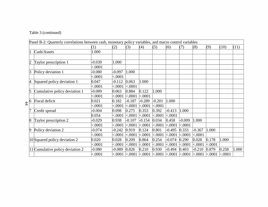
44

Table 3 (continued)

Panel B-2: Quarterly correlations between cash, monetary policy variables, and macro control variables

(1) (2) (3) (4) (5) (6) (7) (8) (9) (10) (11)

1 Cash/Assets 1.000

2 Taylor prescription 1 -0.039 1.000

<.0001

3 Policy deviation 1 -0.080 -0.097 1.000

<.0001 <.0001

4 Squared policy deviation 1 0.047 -0.112 0.063 1.000

<.0001 <.0001 <.0001

5 Cumulative policy deviation 1 -0.089 0.063 0.884 0.122 1.000

<.0001 <.0001 <.0001 <.0001

6 Fiscal deficit 0.021 0.182 -0.187 -0.289 -0.201 1.000

<.0001 <.0001 <.0001 <.0001 <.0001

7 Credit spread -0.004 0.098 0.275 0.353 0.392 -0.413 1.000

0.054 <.0001 <.0001 <.0001 <.0001 <.0001

8 Taylor prescription 2 -0.029 0.938 -0.107 -0.154 0.034 0.458 -0.009 1.000

<.0001 <.0001 <.0001 <.0001 <.0001 <.0001 <.0001

9 Policy deviation 2 -0.074 -0.242 0.919 0.124 0.801 -0.495 0.333 -0.367 1.000

<.0001 <.0001 <.0001 <.0001 <.0001 <.0001 <.0001 <.0001

10 Squared policy deviation 2 0.020 0.028 0.209 0.864 0.254 -0.074 0.290 0.028 0.178 1.000

<.0001 <.0001 <.0001 <.0001 <.0001 <.0001 <.0001 <.0001 <.0001

11 Cumulative policy deviation 2 -0.080 -0.089 0.826 0.210 0.930 -0.494 0.403 -0.210 0.879 0.258 1.000

<.0001 <.0001 <.0001 <.0001 <.0001 <.0001 <.0001 <.0001 <.0001 <.0001

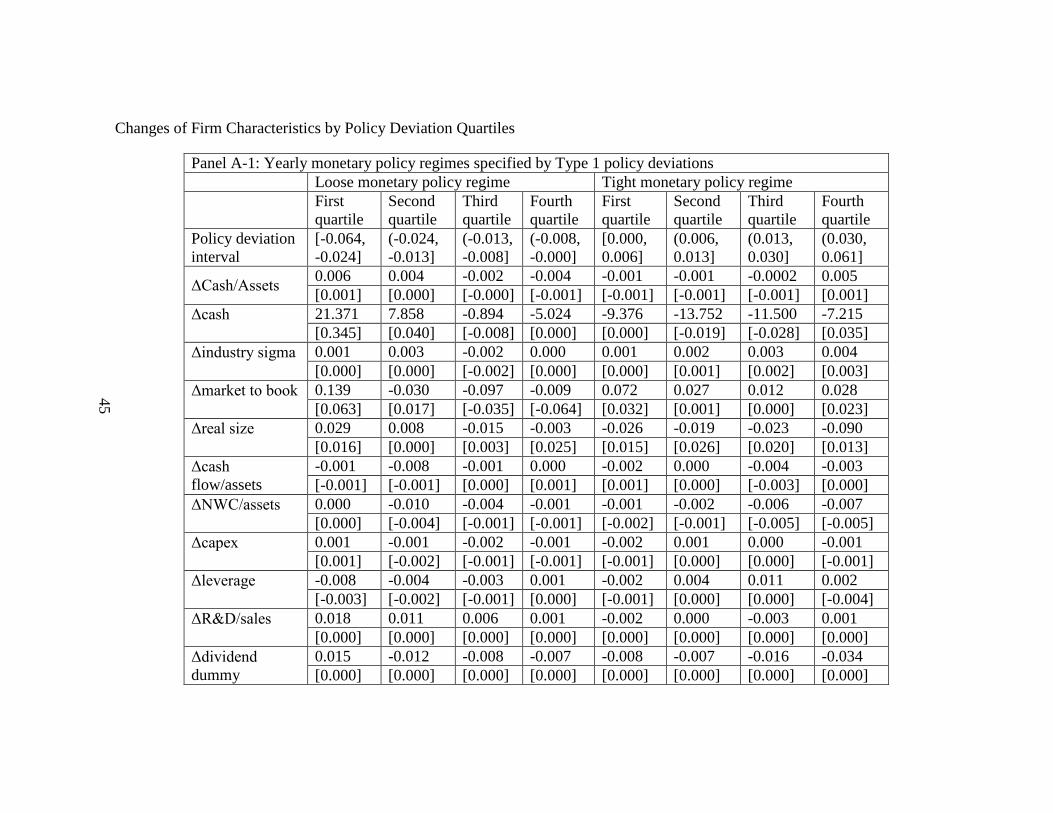
45

Changes of Firm Characteristics by Policy Deviation Quartiles

Panel A-1: Yearly monetary policy regimes specified by Type 1 policy deviations

Loose monetary policy regime Tight monetary policy regime

First

quartile

Second

quartile

Third

quartile

Fourth

quartile

First

quartile

Second

quartile

Third

quartile

Fourth

quartile

Policy deviation

interval

[-0.064,

-0.024]

(-0.024,

-0.013]

(-0.013,

-0.008]

(-0.008,

-0.000]

[0.000,

0.006]

(0.006,

0.013]

(0.013,

0.030]

(0.030,

0.061]

ΔCash/Assets 0.006 0.004 -0.002 -0.004 -0.001 -0.001 -0.0002 0.005

[0.001] [0.000] [-0.000] [-0.001] [-0.001] [-0.001] [-0.001] [0.001]

Δcash

21.371 7.858 -0.894 -5.024 -9.376 -13.752 -11.500 -7.215

[0.345] [0.040] [-0.008] [0.000] [0.000] [-0.019] [-0.028] [0.035]

Δindustry sigma

0.001 0.003 -0.002 0.000 0.001 0.002 0.003 0.004

[0.000] [0.000] [-0.002] [0.000] [0.000] [0.001] [0.002] [0.003]

Δmarket to book

0.139 -0.030 -0.097 -0.009 0.072 0.027 0.012 0.028

[0.063] [0.017] [-0.035] [-0.064] [0.032] [0.001] [0.000] [0.023]

Δreal size

0.029 0.008 -0.015 -0.003 -0.026 -0.019 -0.023 -0.090

[0.016] [0.000] [0.003] [0.025] [0.015] [0.026] [0.020] [0.013]

Δcash

flow/assets

-0.001 -0.008 -0.001 0.000 -0.002 0.000 -0.004 -0.003

[-0.001] [-0.001] [0.000] [0.001] [0.001] [0.000] [-0.003] [0.000]

ΔNWC/assets

0.000 -0.010 -0.004 -0.001 -0.001 -0.002 -0.006 -0.007

[0.000] [-0.004] [-0.001] [-0.001] [-0.002] [-0.001] [-0.005] [-0.005]

Δcapex

0.001 -0.001 -0.002 -0.001 -0.002 0.001 0.000 -0.001

[0.001] [-0.002] [-0.001] [-0.001] [-0.001] [0.000] [0.000] [-0.001]

Δleverage

-0.008 -0.004 -0.003 0.001 -0.002 0.004 0.011 0.002

[-0.003] [-0.002] [-0.001] [0.000] [-0.001] [0.000] [0.000] [-0.004]

ΔR&D/sales

0.018 0.011 0.006 0.001 -0.002 0.000 -0.003 0.001

[0.000] [0.000] [0.000] [0.000] [0.000] [0.000] [0.000] [0.000]

Δdividend

dummy

0.015 -0.012 -0.008 -0.007 -0.008 -0.007 -0.016 -0.034

[0.000] [0.000] [0.000] [0.000] [0.000] [0.000] [0.000] [0.000]

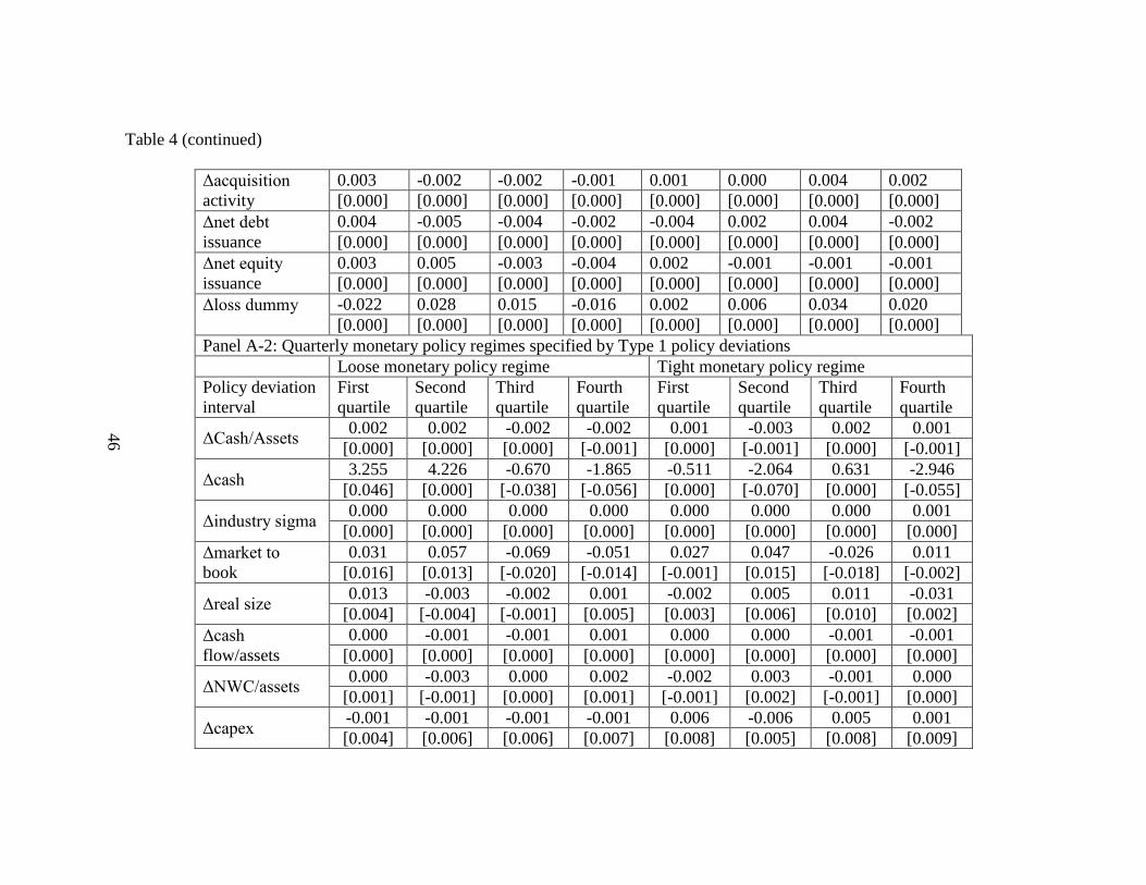
46

Table 4 (continued)

Δacquisition

activity

0.003 -0.002 -0.002 -0.001 0.001 0.000 0.004 0.002

[0.000] [0.000] [0.000] [0.000] [0.000] [0.000] [0.000] [0.000]

Δnet debt

issuance

0.004 -0.005 -0.004 -0.002 -0.004 0.002 0.004 -0.002

[0.000] [0.000] [0.000] [0.000] [0.000] [0.000] [0.000] [0.000]

Δnet equity

issuance

0.003 0.005 -0.003 -0.004 0.002 -0.001 -0.001 -0.001

[0.000] [0.000] [0.000] [0.000] [0.000] [0.000] [0.000] [0.000]

Δloss dummy

-0.022 0.028 0.015 -0.016 0.002 0.006 0.034 0.020

[0.000] [0.000] [0.000] [0.000] [0.000] [0.000] [0.000] [0.000]

Panel A-2: Quarterly monetary policy regimes specified by Type 1 policy deviations

Loose monetary policy regime Tight monetary policy regime

Policy deviation

interval

First

quartile

Second

quartile

Third

quartile

Fourth

quartile

First

quartile

Second

quartile

Third

quartile

Fourth

quartile

ΔCash/Assets 0.002 0.002 -0.002 -0.002 0.001 -0.003 0.002 0.001

[0.000] [0.000] [0.000] [-0.001] [0.000] [-0.001] [0.000] [-0.001]

Δcash 3.255 4.226 -0.670 -1.865 -0.511 -2.064 0.631 -2.946

[0.046] [0.000] [-0.038] [-0.056] [0.000] [-0.070] [0.000] [-0.055]

Δindustry sigma 0.000 0.000 0.000 0.000 0.000 0.000 0.000 0.001

[0.000] [0.000] [0.000] [0.000] [0.000] [0.000] [0.000] [0.000]

Δmarket to

book

0.031 0.057 -0.069 -0.051 0.027 0.047 -0.026 0.011

[0.016] [0.013] [-0.020] [-0.014] [-0.001] [0.015] [-0.018] [-0.002]

Δreal size 0.013 -0.003 -0.002 0.001 -0.002 0.005 0.011 -0.031

[0.004] [-0.004] [-0.001] [0.005] [0.003] [0.006] [0.010] [0.002]

Δcash

flow/assets

0.000 -0.001 -0.001 0.001 0.000 0.000 -0.001 -0.001

[0.000] [0.000] [0.000] [0.000] [0.000] [0.000] [0.000] [0.000]

ΔNWC/assets 0.000 -0.003 0.000 0.002 -0.002 0.003 -0.001 0.000

[0.001] [-0.001] [0.000] [0.001] [-0.001] [0.002] [-0.001] [0.000]

Δcapex -0.001 -0.001 -0.001 -0.001 0.006 -0.006 0.005 0.001

[0.004] [0.006] [0.006] [0.007] [0.008] [0.005] [0.008] [0.009]

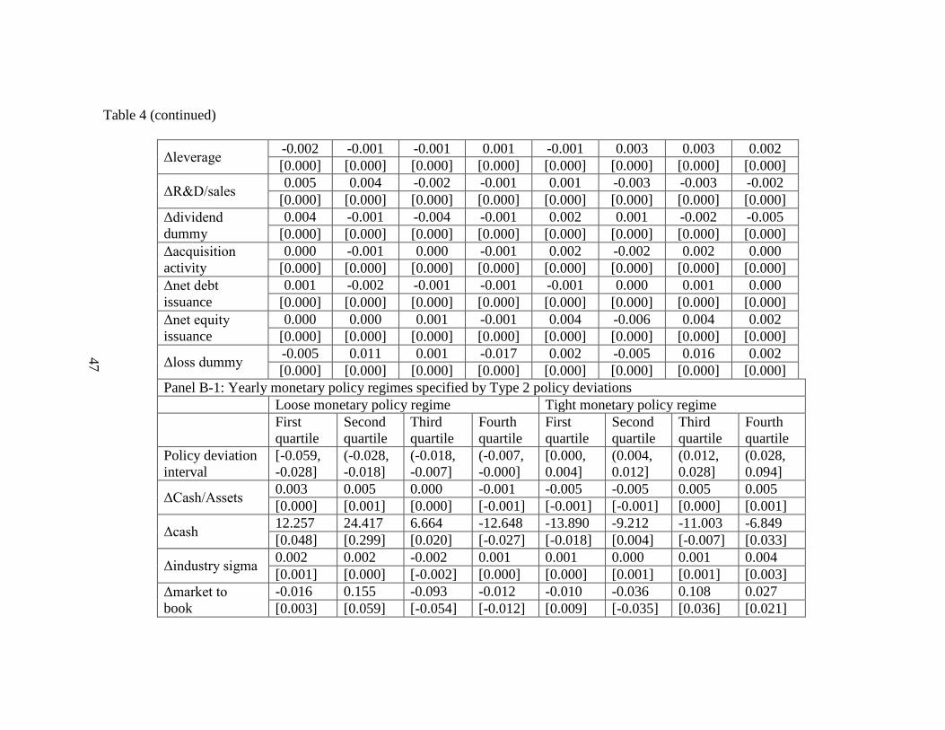
47

Table 4 (continued)

Δleverage -0.002 -0.001 -0.001 0.001 -0.001 0.003 0.003 0.002

[0.000] [0.000] [0.000] [0.000] [0.000] [0.000] [0.000] [0.000]

ΔR&D/sales 0.005 0.004 -0.002 -0.001 0.001 -0.003 -0.003 -0.002

[0.000] [0.000] [0.000] [0.000] [0.000] [0.000] [0.000] [0.000]

Δdividend

dummy

0.004 -0.001 -0.004 -0.001 0.002 0.001 -0.002 -0.005

[0.000] [0.000] [0.000] [0.000] [0.000] [0.000] [0.000] [0.000]

Δacquisition

activity

0.000 -0.001 0.000 -0.001 0.002 -0.002 0.002 0.000

[0.000] [0.000] [0.000] [0.000] [0.000] [0.000] [0.000] [0.000]

Δnet debt

issuance

0.001 -0.002 -0.001 -0.001 -0.001 0.000 0.001 0.000

[0.000] [0.000] [0.000] [0.000] [0.000] [0.000] [0.000] [0.000]

Δnet equity

issuance

0.000 0.000 0.001 -0.001 0.004 -0.006 0.004 0.002

[0.000] [0.000] [0.000] [0.000] [0.000] [0.000] [0.000] [0.000]

Δloss dummy -0.005 0.011 0.001 -0.017 0.002 -0.005 0.016 0.002

[0.000] [0.000] [0.000] [0.000] [0.000] [0.000] [0.000] [0.000]

Panel B-1: Yearly monetary policy regimes specified by Type 2 policy deviations

Loose monetary policy regime Tight monetary policy regime

First

quartile

Second

quartile

Third

quartile

Fourth

quartile

First

quartile

Second

quartile

Third

quartile

Fourth

quartile

Policy deviation

interval

[-0.059,

-0.028]

(-0.028,

-0.018]

(-0.018,

-0.007]

(-0.007,

-0.000]

[0.000,

0.004]

(0.004,

0.012]

(0.012,

0.028]

(0.028,

0.094]

ΔCash/Assets 0.003 0.005 0.000 -0.001 -0.005 -0.005 0.005 0.005

[0.000] [0.001] [0.000] [-0.001] [-0.001] [-0.001] [0.000] [0.001]

Δcash 12.257 24.417 6.664 -12.648 -13.890 -9.212 -11.003 -6.849

[0.048] [0.299] [0.020] [-0.027] [-0.018] [0.004] [-0.007] [0.033]

Δindustry sigma 0.002 0.002 -0.002 0.001 0.001 0.000 0.001 0.004

[0.001] [0.000] [-0.002] [0.000] [0.000] [0.001] [0.001] [0.003]

Δmarket to

book

-0.016 0.155 -0.093 -0.012 -0.010 -0.036 0.108 0.027

[0.003] [0.059] [-0.054] [-0.012] [0.009] [-0.035] [0.036] [0.021]

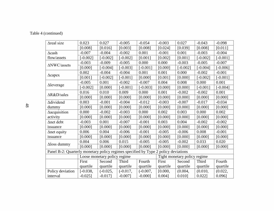
48

Table 4 (continued)

Δreal size

0.023 0.027 -0.005 -0.054 -0.003 0.027 -0.043 -0.098

[0.008] [0.016] [0.003] [0.008] [0.024] [0.039] [0.008] [0.011]

Δcash

flow/assets

-0.007 -0.004 -0.002 0.001 -0.001 0.001 -0.003 -0.004

[-0.002] [-0.002] [-0.002] [0.001] [0.002] [0.001] [-0.002] [-0.001]

ΔNWC/assets -0.003 -0.009 -0.005 0.000 0.000 -0.003 -0.005 -0.007

[0.000] [-0.004] [-0.003] [-0.001] [0.000] [-0.002] [-0.004] [-0.006]

Δcapex 0.002 -0.004 -0.004 0.001 0.001 0.000 -0.002 -0.001

[0.001] [-0.002] [-0.001] [0.000] [0.001] [0.000] [-0.002] [-0.001]

Δleverage -0.005 0.001 -0.002 -0.007 0.004 0.008 0.000 0.001

[-0.002] [0.000] [-0.001] [-0.003] [0.000] [0.000] [-0.001] [-0.004]

ΔR&D/sales 0.016 0.010 0.009 0.000 0.001 -0.002 -0.002 0.001

[0.000] [0.000] [0.000] [0.000] [0.000] [0.000] [0.000] [0.000]

Δdividend

dummy

0.003 -0.001 -0.004 -0.012 -0.003 -0.007 -0.017 -0.034

[0.000] [0.000] [0.000] [0.000] [0.000] [0.000] [0.000] [0.000]

Δacquisition

activity

0.000 -0.002 -0.003 0.000 0.002 0.003 0.000 0.002

[0.000] [0.000] [0.000] [0.000] [0.000] [0.000] [0.000] [0.000]

Δnet debt

issuance

-0.003 0.001 -0.007 -0.001 0.003 0.004 -0.002 -0.002

[0.000] [0.000] [0.000] [0.000] [0.000] [0.000] [0.000] [0.000]

Δnet equity

issuance

0.006 0.004 -0.006 -0.001 -0.005 -0.006 0.008 -0.001

[0.000] [0.000] [0.000] [0.000] [0.000] [0.000] [0.000] [0.000]

Δloss dummy 0.004 0.006 0.015 -0.005 -0.005 -0.002 0.033 0.020

[0.000] [0.000] [0.000] [0.000] [0.000] [0.000] [0.000] [0.000]

Panel B-2: Quarterly monetary policy regimes specified by Type 2 policy deviations

Loose monetary policy regime Tight monetary policy regime

First

quartile

Second

quartile

Third

quartile

Fourth

quartile

First

quartile

Second

quartile

Third

quartile

Fourth

quartile

Policy deviation

interval

[-0.038,

-0.025]

(-0.025,

-0.017]

(-0.017,

-0.007]

(-0.007,

-0.000]

[0.000,

0.004]

(0.004,

0.010]

(0.010,

0.022]

(0.022,

0.096]

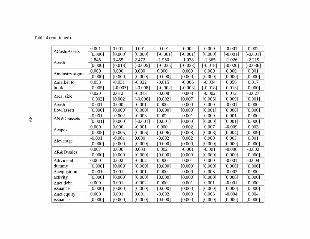
49

Table 4 (continued)

ΔCash/Assets 0.001 0.001 0.001 -0.001 -0.002 0.000 -0.001 0.002

[0.000] [0.000] [0.000] [-0.001] [-0.001] [0.000] [-0.001] [-0.001]

Δcash 2.845 3.455 2.472 -1.950 -1.078 -1.365 -1.026 -2.219

[0.000] [0.013] [-0.005] [-0.035] [-0.038] [-0.018] [-0.020] [-0.036]

Δindustry sigma 0.000 0.000 0.000 0.000 0.000 0.000 0.000 0.001

[0.000] [0.000] [0.000] [0.000] [0.000] [0.000] [0.000] [0.000]

Δmarket to

book

0.053 -0.031 -0.022 -0.015 -0.006 -0.034 0.050 0.017

[0.005] [-0.003] [-0.008] [-0.002] [-0.003] [-0.018] [0.013] [0.000]

Δreal size 0.020 0.012 -0.013 -0.008 0.003 -0.002 0.012 -0.027

[0.003] [0.002] [-0.006] [0.002] [0.007] [0.005] [0.009] [0.001]

Δcash

flow/assets

-0.001 0.000 -0.001 0.000 0.000 0.000 -0.001 0.000

[0.000] [0.000] [0.000] [0.000] [0.000] [0.001] [0.000] [0.000]

ΔNWC/assets -0.001 -0.002 -0.003 0.002 0.001 0.000 0.001 0.000

[0.001] [0.000] [-0.001] [0.001] [0.000] [0.000] [0.001] [0.000]

Δcapex 0.000 0.000 -0.001 0.000 0.002 0.007 -0.009 0.003

[0.005] [0.005] [0.006] [0.006] [0.008] [0.008] [0.004] [0.009]

Δleverage -0.001 -0.001 0.000 -0.002 0.002 0.000 0.003 0.001

[0.000] [0.000] [0.000] [0.000] [0.000] [0.000] [0.000] [0.000]

ΔR&D/sales 0.007 0.000 0.003 0.002 -0.001 -0.001 -0.006 -0.002

[0.000] [0.000] [0.000] [0.000] [0.000] [0.000] [0.000] [0.000]

Δdividend

dummy

0.000 0.002 -0.002 0.000 0.001 0.000 -0.001 -0.004

[0.000] [0.000] [0.000] [0.000] [0.000] [0.000] [0.000] [0.000]

Δacquisition

activity

-0.001 0.001 -0.001 0.000 0.000 0.003 -0.002 0.000

[0.000] [0.000] [0.000] [0.000] [0.000] [0.000] [0.000] [0.000]

Δnet debt

issuance

0.000 0.001 -0.002 0.000 0.001 0.001 -0.001 0.000

[0.000] [0.000] [0.000] [0.000] [0.000] [0.000] [0.000] [0.000]

Δnet equity

issuance

0.000 0.001 0.001 -0.002 0.000 0.003 -0.004 0.004

[0.000] [0.000] [0.000] [0.000] [0.000] [0.000] [0.000] [0.000]

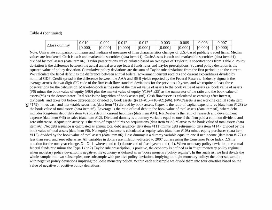
50

Table 4 (continued)

Δloss dummy 0.010 -0.002 0.012 -0.012 -0.003 -0.009 0.003 0.007

[0.000] [0.000] [0.000] [0.000] [0.000] [0.000] [0.000] [0.000] Note: Univariate comparison of means and medians of measures of firm characteristics changes of U.S.-based publicly traded firms. Median

values are bracketed. Cash is cash and marketable securities (data item #1). Cash/Assets is cash and marketable securities (data item #1)

divided by total assets (data item #6). Taylor prescriptions are calculated based on two types of Taylor rule specifications from Table 2. Policy

deviation is the difference between the actual annual average federal funds rates and Taylor prescriptions. Squared policy deviation is the

squared value of policy deviation. Cumulative policy deviations are the sum of Taylor rule deviations from the first period up to the current.

We calculate the fiscal deficit as the difference between annual federal government current receipts and current expenditures divided by

nominal GDP. Credit spread is the difference between the AAA and BBB yields reported by the Federal Reserve. Industry sigma is the

average across the two-digit SIC code of the firm cash flow standard deviations for the previous 10 years, and we require at least three

observations for the calculation. Market-to-book is the ratio of the market value of assets to the book value of assets i.e. book value of assets

(#6) minus the book value of equity (#60) plus the market value of equity (#199* #25) as the numerator of the ratio and the book value of

assets (#6) as the denominator. Real size is the logarithm of book assets (#6). Cash flow/assets is calculated as earnings after interest,

dividends, and taxes but before depreciation divided by book assets (((#13–#15–#16–#21)/#6). NWC/assets is net working capital (data item

#179) minus cash and marketable securities (data item #1) divided by book assets. Capex is the ratio of capital expenditures (data item #128) to

the book value of total assets (data item #6). Leverage is the ratio of total debt to the book value of total assets (data item #6), where debt

includes long-term debt (data item #9) plus debt in current liabilities (data item #34). R&D/sales is the ratio of research and development

expense (data item #46) to sales (data item #12). Dividend dummy is a dummy variable equal to one if the firm paid a common dividend and

zero otherwise. Acquisition activity is the ratio of expenditures on acquisitions (data item #129) relative to the book value of total assets (data

item #6). Net debt issuance is calculated as annual total debt issuance (data item #111) minus debt retirement (data item #114), divided by the

book value of total assets (data item #6). Net equity issuance is calculated as equity sales (data item #108) minus equity purchases (data item

#115), divided by the book value of total assets (data item #6). Loss dummy is a dummy variable equal to one if net income (data item #172) is

less than zero, and zero otherwise. All variables in dollars are inflation-adjusted to 2007 dollars using the Consumer Price Index. ΔXt is

notation for the one-year change, Xt- Xt-1, where t and (t-1) denote end of fiscal year t and (t-1). When monetary policy deviation, the actual

federal funds rate minus the Type 1 (or 2) Taylor rule prescription, is positive, the economy is defined as in “tight monetary policy regime”;

when monetary policy deviation is negative, the economy is defined as in “loose monetary policy regime”. In this analysis, we first divide the

whole sample into two subsamples, one subsample with positive policy deviations implying too tight monetary policy; the other subsample

with negative policy deviations implying too loose monetary policy. Within each subsample we divide them into four quartiles based on the

value of negative or positive policy deviations.

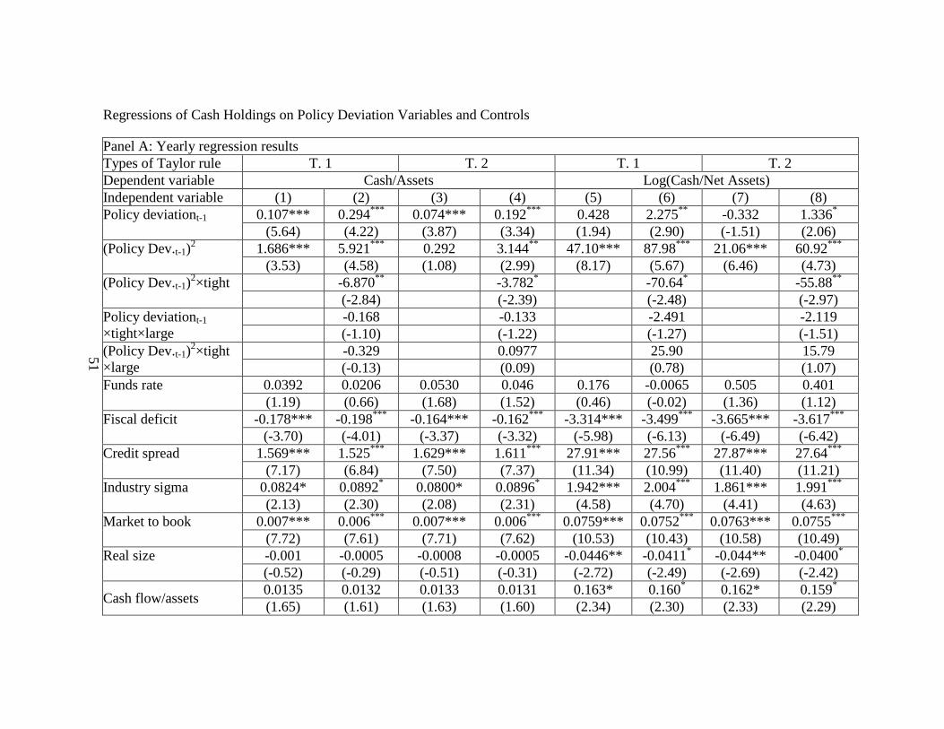
51

Regressions of Cash Holdings on Policy Deviation Variables and Controls

Panel A: Yearly regression results

Types of Taylor rule T. 1 T. 2 T. 1 T. 2

Dependent variable Cash/Assets Log(Cash/Net Assets)

Independent variable (1) (2) (3) (4) (5) (6) (7) (8)

Policy deviationt-1 0.107*** 0.294***

0.074*** 0.192***

0.428 2.275**

-0.332 1.336*

(5.64) (4.22) (3.87) (3.34) (1.94) (2.90) (-1.51) (2.06)

(Policy Dev.t-1)2 1.686*** 5.921

*** 0.292 3.144

** 47.10*** 87.98

*** 21.06*** 60.92

***

(3.53) (4.58) (1.08) (2.99) (8.17) (5.67) (6.46) (4.73)

(Policy Dev.t-1)2×tight -6.870

** -3.782

* -70.64

* -55.88

**

(-2.84) (-2.39) (-2.48) (-2.97)

Policy deviationt-1

×tight×large

-0.168 -0.133 -2.491 -2.119

(-1.10) (-1.22) (-1.27) (-1.51)

(Policy Dev.t-1)2×tight

×large

-0.329 0.0977 25.90 15.79

(-0.13) (0.09) (0.78) (1.07)

Funds rate 0.0392 0.0206 0.0530 0.046 0.176 -0.0065 0.505 0.401

(1.19) (0.66) (1.68) (1.52) (0.46) (-0.02) (1.36) (1.12)

Fiscal deficit -0.178*** -0.198***

-0.164*** -0.162***

-3.314*** -3.499***

-3.665*** -3.617***

(-3.70) (-4.01) (-3.37) (-3.32) (-5.98) (-6.13) (-6.49) (-6.42)

Credit spread 1.569*** 1.525***

1.629*** 1.611***

27.91*** 27.56***

27.87*** 27.64***

(7.17) (6.84) (7.50) (7.37) (11.34) (10.99) (11.40) (11.21)

Industry sigma 0.0824* 0.0892* 0.0800* 0.0896

* 1.942*** 2.004

*** 1.861*** 1.991

***

(2.13) (2.30) (2.08) (2.31) (4.58) (4.70) (4.41) (4.63)

Market to book 0.007*** 0.006***

0.007*** 0.006***

0.0759*** 0.0752***

0.0763*** 0.0755***

(7.72) (7.61) (7.71) (7.62) (10.53) (10.43) (10.58) (10.49)

Real size -0.001 -0.0005 -0.0008 -0.0005 -0.0446** -0.0411* -0.044** -0.0400

*

(-0.52) (-0.29) (-0.51) (-0.31) (-2.72) (-2.49) (-2.69) (-2.42)

Cash flow/assets 0.0135 0.0132 0.0133 0.0131 0.163* 0.160

* 0.162* 0.159

*

(1.65) (1.61) (1.63) (1.60) (2.34) (2.30) (2.33) (2.29)

52

Table 5 (continued)

NWC/assets -0.263*** -0.263***

-0.263*** -0.263***

-2.257*** -2.263***

-2.254*** -2.263***

(-34.47) (-34.50) (-34.46) (-34.47) (-30.76) (-30.78) (-30.72) (-30.75)

Capex -0.367*** -0.368

*** -0.366*** -0.368

*** -2.983*** -2.994

*** -2.971*** -2.990

***

(-27.13) (-27.19) (-27.09) (-27.15) (-20.87) (-20.93) (-20.78) (-20.89)

Leverage -0.247*** -0.248***

-0.247*** -0.247***

-2.805*** -2.813***

-2.808*** -2.815***

(-33.34) (-33.39) (-33.35) (-33.38) (-36.36) (-36.39) (-36.39) (-36.44)

R&D/sales 0.016*** 0.0159

*** 0.0158*** 0.0158

*** 0.0989*** 0.0993

*** 0.099*** 0.0995

***

(3.50) (3.51) (3.50) (3.51) (3.74) (3.76) (3.75) (3.77)

Dividend dummy -0.0005 -0.0004 -0.0004 -0.0004 -0.0262 -0.0260 -0.0254 -0.0259

(-0.18) (-0.16) (-0.16) (-0.15) (-0.91) (-0.90) (-0.88) (-0.89)

Acquisition activity -0.285*** -0.286

*** -0.285*** -0.286

*** -2.086*** -2.091

*** -2.071*** -2.077

***

(-26.00) (-26.01) (-25.94) (-25.95) (-16.64) (-16.67) (-16.50) (-16.54)

Net debt issuance 0.159*** 0.159***

0.159*** 0.159***

1.188*** 1.188***

1.190*** 1.189***

(15.37) (15.37) (15.37) (15.37) (12.53) (12.52) (12.53) (12.53)

Net equity issuance 0.174*** 0.174

*** 0.174*** 0.174

*** 1.141*** 1.138

*** 1.140*** 1.137

***

(23.02) (22.98) (23.02) (22.99) (18.96) (18.90) (18.93) (18.88)

Loss dummy -0.0234*** -0.0234***

-0.0235*** -0.0234***

-0.223*** -0.223***

-0.224*** -0.223***

(-17.64) (-17.61) (-17.66) (-17.63) (-14.70) (-14.69) (-14.75) (-14.72)

Intercept 0.223*** 0.222***

0.223*** 0.221***

-1.912*** -1.920***

-1.926*** -1.948***

(21.65) (21.55) (21.55) (21.23) (-17.69) (-17.74) (-17.81) (-17.84)

Within R2 0.214 0.214 0.213 0.214 0.162 0.162 0.162 0.162

Panel B: Quarterly regression results

Types of Taylor rule T. 1 T. 2 T. 1 T. 2

Dependent variable Cash/Assets Log(Cash/Net Assets)

Independent variable (1) (2) (3) (4) (5) (6) (7) (8)

Policy deviationt-1 0.0359 0.323*** -0.001 0.181** -0.659 4.719*** -0.994** 1.703**

(1.03) (5.06) (-0.04) (3.25) (-1.69) (6.65) (-2.83) (2.73)

53

Table 5 (continued)

(Policy Dev.t-1)2 4.596*** 15.44*** 1.915** 8.059*** 78.60*** 294.3*** 29.42*** 127.1***

(5.00) (6.01) (3.19) (3.97) (7.56) (10.16) (4.36) (5.46)

(Policy Dev.t-1)2×tight -15.66*** -7.783** -336.0*** -133.7***

(-4.48) (-3.00) (-8.52) (-4.54)

Policy deviationt-1

×tight×large

-0.668*** -0.608*** -8.650*** -7.135***

(-4.44) (-4.97) (-4.31) (-4.44)

(Policy Dev.t-1)2×tight

×large

4.376 3.675* 116.9** 71.78**

(1.51) (2.09) (3.10) (3.20)

Funds rate 0.163*** 0.160*** 0.171*** 0.167*** 0.732 0.617 0.680 0.578

(4.66) (4.54) (4.92) (4.77) (1.80) (1.51) (1.69) (1.42)

Fiscal deficit -0.236*** -0.225*** -0.266*** -0.266*** -3.292*** -2.989*** -4.149*** -4.110***

(-4.99) (-4.67) (-5.56) (-5.54) (-5.91) (-5.29) (-7.35) (-7.25)

Credit spread 1.774*** 1.935*** 1.877*** 1.992*** 27.95*** 31.00*** 29.45*** 31.17***

(7.07) (7.53) (7.42) (7.66) (9.78) (10.58) (10.23) (10.52)

Industry sigma -0.190 -0.188 -0.200* -0.204* -1.661 -1.581 -1.923 -1.978

(-1.88) (-1.87) (-1.98) (-2.02) (-1.57) (-1.50) (-1.82) (-1.87)

Market to book 0.007*** 0.007*** 0.007*** 0.007*** 0.0818*** 0.081*** 0.0828*** 0.082***

(9.95) (9.84) (10.01) (9.87) (13.13) (12.98) (13.25) (13.07)

Real size 0.000643 0.000647 0.0008 0.00105 -0.0330 -0.0360* -0.0297 -0.0279

(0.38) (0.38) (0.49) (0.62) (-1.92) (-2.09) (-1.72) (-1.62)

Cash flow/assets -0.0580*** -0.0582*** -0.058*** -0.059*** -0.0894 -0.0883 -0.0935 -0.0956

(-3.36) (-3.37) (-3.37) (-3.40) (-0.62) (-0.62) (-0.65) (-0.67)

NWC/assets -0.242*** -0.242*** -0.242*** -0.242*** -2.106*** -2.098*** -2.108*** -2.104***

(-30.27) (-30.28) (-30.25) (-30.27) (-28.72) (-28.70) (-28.73) (-28.71)

Capex -0.206*** -0.207*** -0.206*** -0.207*** -1.075*** -1.077*** -1.082*** -1.091***

(-20.07) (-20.09) (-20.02) (-20.09) (-9.83) (-9.86) (-9.87) (-9.96)

Leverage -0.245*** -0.245*** -0.246*** -0.246*** -2.788*** -2.781*** -2.799*** -2.798***

(-31.83) (-31.83) (-31.90) (-31.92) (-35.83) (-35.80) (-35.95) (-35.96)

54

Table 5 (continued)

R&D/sales 0.009*** 0.009*** 0.009*** 0.009*** 0.0573*** 0.058*** 0.0573*** 0.058***

(3.82) (3.85) (3.82) (3.85) (4.08) (4.10) (4.08) (4.12)

Dividend dummy -0.00466* -0.00428* -0.00465* -0.00422* -0.0718* -0.0688* -0.0716* -0.0676*

(-2.17) (-2.00) (-2.16) (-1.96) (-2.50) (-2.40) (-2.48) (-2.35)

Acquisition activity -0.237*** -0.238*** -0.237*** -0.237*** -1.341*** -1.360*** -1.333*** -1.335***

(-23.20) (-23.26) (-23.11) (-23.11) (-11.26) (-11.42) (-11.18) (-11.19)

Net debt issuance 0.160*** 0.160*** 0.161*** 0.161*** 1.091*** 1.089*** 1.099*** 1.100***

(15.83) (15.83) (15.85) (15.86) (13.00) (12.99) (13.06) (13.07)

Net equity issuance 0.184*** 0.184*** 0.183*** 0.183*** 1.209*** 1.215*** 1.205*** 1.202***

(22.45) (22.46) (22.43) (22.41) (20.58) (20.64) (20.54) (20.51)

Loss dummy -0.0108*** -0.0108*** -0.011*** -0.011*** -0.130*** -0.130*** -0.130*** -0.130***

(-11.22) (-11.25) (-11.24) (-11.25) (-12.00) (-12.03) (-12.02) (-12.04)

Intercept 0.199*** 0.198*** 0.197*** 0.196*** -2.055*** -2.058*** -2.080*** -2.097***

(19.54) (19.43) (19.36) (19.17) (-18.90) (-18.96) (-19.14) (-19.31)

Within R2 0.183 0.184 0.183 0.184 0.129 0.130 0.129 0.129

Note: Cash/Assets defined as cash and marketable securities (data item #1) divided by total assets (data item #6). Log net cash ratio defined as log value of cash and marketable securities (data item

#1) divided by (total assets (data item #6)-cash and marketable securities (data item #1)). The sample includes all Compustat firm-year observations from 1980 to 2007 with positive values for the book value of total assets and sales revenue for firms incorporated in the United States. Financial firms (SIC code 6000-6999) and utilities (SIC codes 4900-4999) are excluded from the sample,

yielding a panel of 118,897 observations for 13,743 unique firms. Missing explanatory values reduce the panel used here to 67,066 firm-year observations for 12,430 unique firms for the firm fixed

effects regressions. Taylor prescriptions are calculated based on two types of Taylor rule specifications from Table 2. Policy deviation is the difference between the actual annual average federal

funds rates and Taylor prescriptions. Squared policy deviation is the squared value of policy deviation. We calculate the fiscal deficit as the difference between annual federal government current

receipts and current expenditures divided by nominal GDP. Credit spread is the difference between the AAA and BBB yields reported by the Federal Reserve. Industry sigma is the average across

the two-digit SIC code of the firm cash flow standard deviations for the previous 10 years, and we require at least three observations for the calculation. Market-to-book is the ratio of the market value of assets to the book value of assets i.e. book value of assets (#6) minus the book value of equity (#60) plus the market value of equity (#199* #25) as the numerator of the ratio and the book

value of assets (#6) as the denominator. Real size is the logarithm of book assets (#6). Cash flow/assets is calculated as earnings after interest, dividends, and taxes but before depreciation divided by

book assets (((#13–#15–#16–#21)/#6). NWC/assets is net working capital (data item #179) minus cash and marketable securities (data item #1) divided by book assets. Capex is the ratio of capital expenditures (data item #128) to the book value of total assets (data item #6). Leverage is the ratio of total debt to the book value of total assets (data item #6), where debt includes long-term debt

(data item #9) plus debt in current liabilities (data item #34). R&D/sales is the ratio of research and development expense (data item #46) to sales (data item #12). Dividend dummy is a dummy

variable equal to one if the firm paid a common dividend and zero otherwise. Acquisition activity is the ratio of expenditures on acquisitions (data item #129) relative to the book value of total assets (data item #6). Net debt issuance is calculated as annual total debt issuance (data item #111) minus debt retirement (data item #114), divided by the book value of total assets (data item #6).

Net equity issuance is calculated as equity sales (data item #108) minus equity purchases (data item #115), divided by the book value of total assets (data item #6). Loss dummy is a dummy variable

equal to one if net income (data item #172) is less than zero, and zero otherwise. 2000s dummy is a dummy variable equal to one if the firm observation is in the fiscal year after 1999, and zero otherwise. All variables in dollars are inflation-adjusted to 2007 dollars using the Consumer Price Index. ΔXt is notation for the one-year change, Xt- Xt-1, where t and (t-1) denote end of fiscal year t

and (t-1). In this analysis, we first divide the whole sample into four quartiles each fiscal year based on the real size and define firms in the largest real size quartiles as “large” firms. Large is a

dummy variable equal to one if the firm is in the large real size quartile and zero otherwise. t-statistics based on standard errors robust to clustering by firm and year are reported in parentheses. We

report adjusted-R2 for OLS estimation models and within R2 for firm fixed effects estimation models. ***, **, and * denote significance at the 1%, 5%, and 10% levels, respectively.

55

Regressions of Cash Holdings on One Year Cumulative Policy Deviation Variables and Controls

Panel A: Yearly regression results

Types of Taylor rule T. 1 T. 2 T. 1 T. 2

Dependent variable Cash/Assets Log(Cash/Net Assets)

Independent variable (1) (2) (3) (4) (5) (6) (7) (8)

Cumulative policy deviation

×large×2000s dummy

0.0182 0.0183 -2.444***

-2.156***

(0.32) (0.33) (-3.64) (-3.32)

Cumulative policy deviation

×large

-0.0134 -0.0209 0.181 0.0537

(-0.97) (-1.67) (0.98) (0.33)

Cumulative policy deviation

×2000s dummy

-0.165***

-0.166***

-2.225***

-2.264***

(-3.92) (-4.13) (-5.13) (-5.29)

Cumulative policy deviation 0.0527*** 0.0797***

0.0468*** 0.0744***

0.212* 0.586***

0.203* 0.577***

(6.47) (7.75) (6.50) (8.07) (2.31) (5.09) (2.49) (5.54)

Funds rate 0.0674* 0.111***

0.0501 0.120***

0.931** 1.726***

0.859* 2.104***

(2.24) (3.85) (1.71) (4.34) (2.60) (5.09) (2.45) (6.37)

Fiscal deficit -0.200*** -0.159***

-0.157*** -0.148**

-3.791*** -3.069***

-3.592*** -3.445***

(-4.38) (-3.34) (-3.41) (-3.19) (-7.13) (-5.50) (-6.71) (-6.38)

Credit spread 1.723*** 1.574***

1.801*** 1.448***

29.19*** 26.54***

29.57*** 23.43***

(7.76) (7.33) (8.11) (7.11) (11.68) (11.05) (11.80) (10.25)

Industry sigma 0.0549 0.0298 0.0634 0.0377 1.597*** 1.179**

1.627*** 1.218**

(1.44) (0.78) (1.67) (0.99) (3.80) (2.77) (3.88) (2.86)

Market to book 0.007*** 0.007***

0.007*** 0.007***

0.077*** 0.0742***

0.076*** 0.0749***

(7.87) (7.72) (7.80) (7.75) (10.61) (10.29) (10.58) (10.42)

Real size -0.00001 -0.00146 -0.0001 -0.00136 -0.0357* -0.0687***

-0.0359* -0.0655***

(-0.00) (-0.87) (-0.07) (-0.82) (-2.17) (-3.97) (-2.19) (-3.82)

Cash flow/assets 0.0135 0.0150 0.0136 0.0149 0.162* 0.190

** 0.162* 0.186

**

(1.65) (1.83) (1.67) (1.83) (2.32) (2.73) (2.33) (2.68)

NWC/assets -0.263*** -0.261***

-0.263*** -0.261***

-2.264*** -2.222***

-2.264*** -2.227***

(-34.51) (-34.18) (-34.53) (-34.26) (-30.82) (-30.11) (-30.83) (-30.22)

56

Table 6 (continued)

Capex -0.368*** -0.364

*** -0.369*** -0.365

*** -2.994*** -2.889

*** -2.998*** -2.903

***

(-27.14) (-26.72) (-27.18) (-26.84) (-20.88) (-20.08) (-20.92) (-20.21)

Leverage -0.249*** -0.247***

-0.249*** -0.247***

-2.833*** -2.798***

-2.832*** -2.803***

(-33.57) (-33.20) (-33.56) (-33.27) (-36.60) (-36.02) (-36.62) (-36.16)

R&D/sales 0.0160*** 0.0158

*** 0.0160*** 0.0159

*** 0.101*** 0.101

*** 0.101*** 0.101

***

(3.55) (3.48) (3.54) (3.49) (3.84) (3.74) (3.84) (3.77)

Dividend dummy -0.0002 -0.00004 -0.0003 0.000004 -0.0219 -0.0194 -0.0220 -0.0178

(-0.09) (-0.02) (-0.10) (0.00) (-0.76) (-0.67) (-0.76) (-0.62)

Acquisition activity -0.287*** -0.289

*** -0.288*** -0.288

*** -2.102*** -2.118

*** -2.106*** -2.097

***

(-26.10) (-26.25) (-26.15) (-26.12) (-16.73) (-16.92) (-16.76) (-16.72)

Net debt issuance 0.159*** 0.159***

0.159*** 0.159***

1.195*** 1.196***

1.194*** 1.194***

(15.38) (15.43) (15.37) (15.40) (12.56) (12.64) (12.55) (12.60)

Net equity issuance 0.175*** 0.177

*** 0.175*** 0.176

*** 1.147*** 1.188

*** 1.147*** 1.170

***

(23.07) (23.29) (23.08) (23.20) (19.06) (19.63) (19.06) (19.38)

Loss dummy -0.0236*** -0.0235***

-0.024*** -0.0235***

-0.226*** -0.223***

-0.226*** -0.224***

(-17.78) (-17.70) (-17.76) (-17.72) (-14.87) (-14.67) (-14.86) (-14.75)

Intercept 0.219*** 0.225***

0.220*** 0.224***

-1.962*** -1.818***

-1.961*** -1.854***

(21.15) (21.43) (21.18) (21.39) (-18.02) (-16.31) (-18.02) (-16.81)

Within R2 0.214 0.215 0.214 0.215 0.161 0.164 0.161 0.164

Panel B: Quarterly regression results

Types of Taylor rule T. 1 T. 2 T. 1 T. 2

Dependent variable Cash/Assets Log(Cash/Net Assets)

Independent variable (1) (2) (3) (4) (5) (6) (7) (8)

Cumulative policy deviation

×large×2000s dummy

0.0580 0.0671* -0.382 0.389

(1.36) (2.08) (-0.70) (0.96)

Cumulative policy deviation

×large

-0.114***

-0.106*** -0.807** -0.853***

(-4.82) (-5.55) (-2.64) (-3.52)

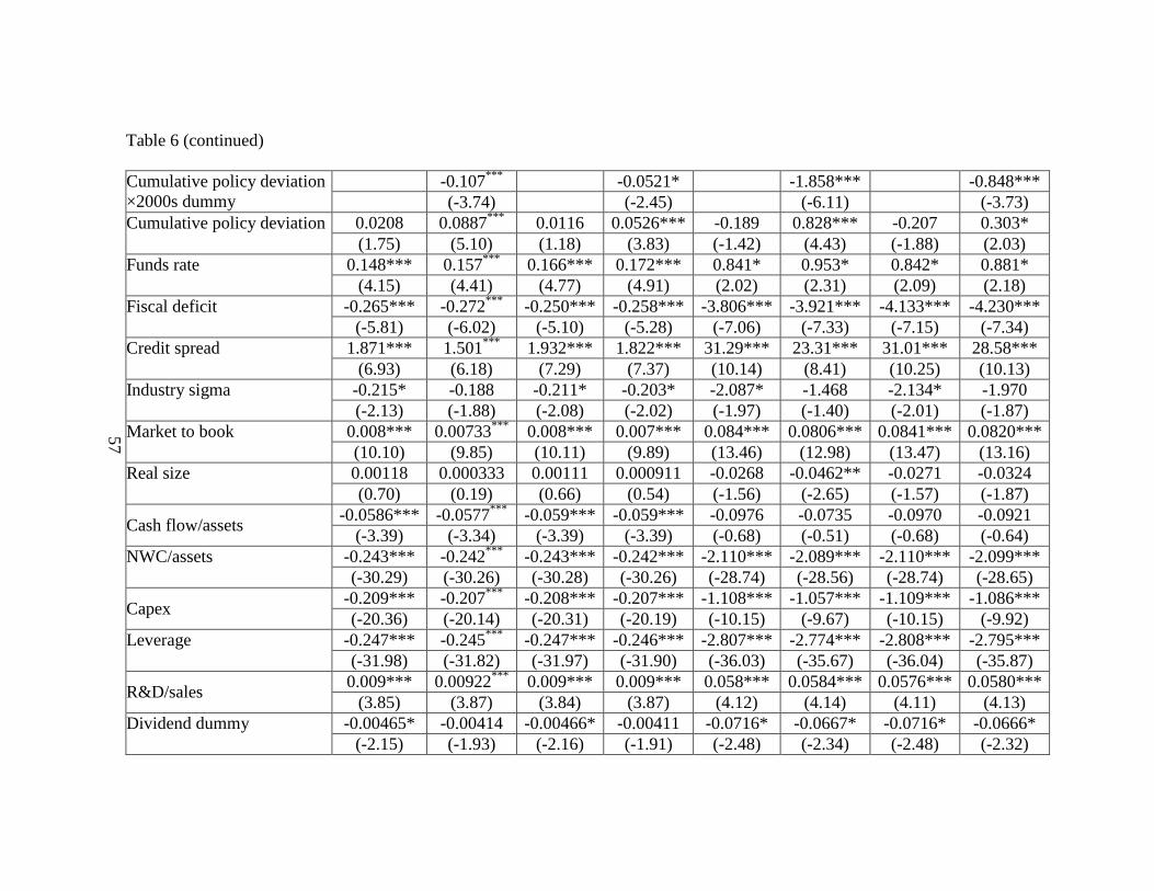
57

Table 6 (continued)

Cumulative policy deviation

×2000s dummy

-0.107***

-0.0521* -1.858*** -0.848***

(-3.74) (-2.45) (-6.11) (-3.73)

Cumulative policy deviation 0.0208 0.0887***

0.0116 0.0526*** -0.189 0.828*** -0.207 0.303*

(1.75) (5.10) (1.18) (3.83) (-1.42) (4.43) (-1.88) (2.03)

Funds rate 0.148*** 0.157***

0.166*** 0.172*** 0.841* 0.953* 0.842* 0.881*

(4.15) (4.41) (4.77) (4.91) (2.02) (2.31) (2.09) (2.18)

Fiscal deficit -0.265*** -0.272***

-0.250*** -0.258*** -3.806*** -3.921*** -4.133*** -4.230***

(-5.81) (-6.02) (-5.10) (-5.28) (-7.06) (-7.33) (-7.15) (-7.34)

Credit spread 1.871*** 1.501***

1.932*** 1.822*** 31.29*** 23.31*** 31.01*** 28.58***

(6.93) (6.18) (7.29) (7.37) (10.14) (8.41) (10.25) (10.13)

Industry sigma -0.215* -0.188 -0.211* -0.203* -2.087* -1.468 -2.134* -1.970

(-2.13) (-1.88) (-2.08) (-2.02) (-1.97) (-1.40) (-2.01) (-1.87)

Market to book 0.008*** 0.00733***

0.008*** 0.007*** 0.084*** 0.0806*** 0.0841*** 0.0820***

(10.10) (9.85) (10.11) (9.89) (13.46) (12.98) (13.47) (13.16)

Real size 0.00118 0.000333 0.00111 0.000911 -0.0268 -0.0462** -0.0271 -0.0324

(0.70) (0.19) (0.66) (0.54) (-1.56) (-2.65) (-1.57) (-1.87)

Cash flow/assets -0.0586*** -0.0577

*** -0.059*** -0.059*** -0.0976 -0.0735 -0.0970 -0.0921

(-3.39) (-3.34) (-3.39) (-3.39) (-0.68) (-0.51) (-0.68) (-0.64)

NWC/assets -0.243*** -0.242***

-0.243*** -0.242*** -2.110*** -2.089*** -2.110*** -2.099***

(-30.29) (-30.26) (-30.28) (-30.26) (-28.74) (-28.56) (-28.74) (-28.65)

Capex -0.209*** -0.207

*** -0.208*** -0.207*** -1.108*** -1.057*** -1.109*** -1.086***

(-20.36) (-20.14) (-20.31) (-20.19) (-10.15) (-9.67) (-10.15) (-9.92)

Leverage -0.247*** -0.245***

-0.247*** -0.246*** -2.807*** -2.774*** -2.808*** -2.795***

(-31.98) (-31.82) (-31.97) (-31.90) (-36.03) (-35.67) (-36.04) (-35.87)

R&D/sales 0.009*** 0.00922

*** 0.009*** 0.009*** 0.058*** 0.0584*** 0.0576*** 0.0580***

(3.85) (3.87) (3.84) (3.87) (4.12) (4.14) (4.11) (4.13)

Dividend dummy -0.00465* -0.00414 -0.00466* -0.00411 -0.0716* -0.0667* -0.0716* -0.0666*

(-2.15) (-1.93) (-2.16) (-1.91) (-2.48) (-2.34) (-2.48) (-2.32)

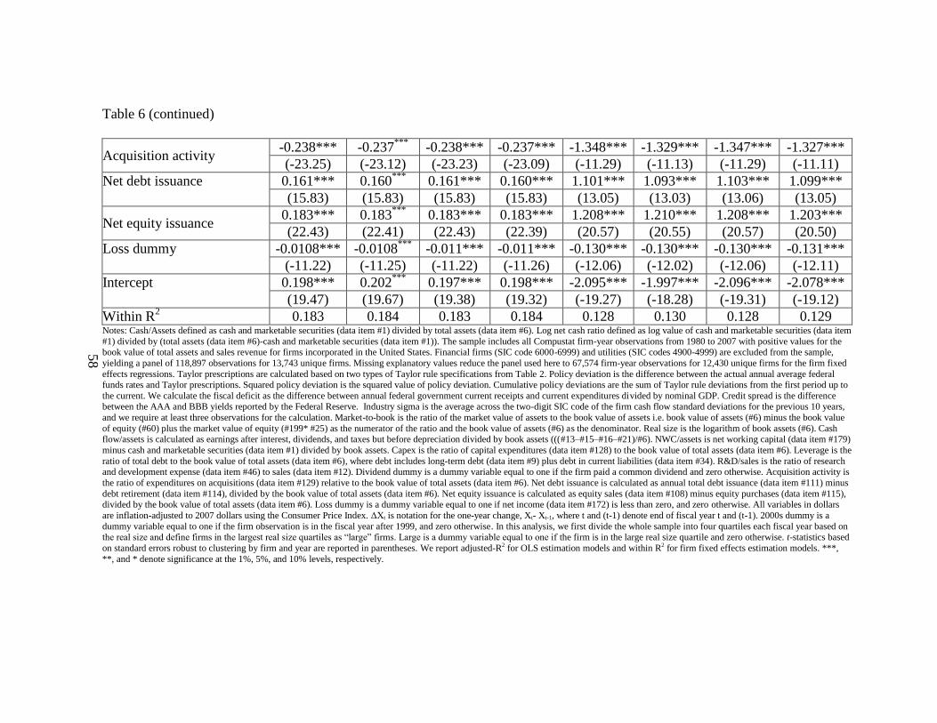
58

Table 6 (continued)

Acquisition activity -0.238*** -0.237

*** -0.238*** -0.237*** -1.348*** -1.329*** -1.347*** -1.327***

(-23.25) (-23.12) (-23.23) (-23.09) (-11.29) (-11.13) (-11.29) (-11.11)

Net debt issuance 0.161*** 0.160***

0.161*** 0.160*** 1.101*** 1.093*** 1.103*** 1.099***

(15.83) (15.83) (15.83) (15.83) (13.05) (13.03) (13.06) (13.05)

Net equity issuance 0.183*** 0.183

*** 0.183*** 0.183*** 1.208*** 1.210*** 1.208*** 1.203***

(22.43) (22.41) (22.43) (22.39) (20.57) (20.55) (20.57) (20.50)

Loss dummy -0.0108*** -0.0108***

-0.011*** -0.011*** -0.130*** -0.130*** -0.130*** -0.131***

(-11.22) (-11.25) (-11.22) (-11.26) (-12.06) (-12.02) (-12.06) (-12.11)

Intercept 0.198*** 0.202***

0.197*** 0.198*** -2.095*** -1.997*** -2.096*** -2.078***

(19.47) (19.67) (19.38) (19.32) (-19.27) (-18.28) (-19.31) (-19.12)

Within R2 0.183 0.184 0.183 0.184 0.128 0.130 0.128 0.129

Notes: Cash/Assets defined as cash and marketable securities (data item #1) divided by total assets (data item #6). Log net cash ratio defined as log value of cash and marketable securities (data item

#1) divided by (total assets (data item #6)-cash and marketable securities (data item #1)). The sample includes all Compustat firm-year observations from 1980 to 2007 with positive values for the book value of total assets and sales revenue for firms incorporated in the United States. Financial firms (SIC code 6000-6999) and utilities (SIC codes 4900-4999) are excluded from the sample,

yielding a panel of 118,897 observations for 13,743 unique firms. Missing explanatory values reduce the panel used here to 67,574 firm-year observations for 12,430 unique firms for the firm fixed

effects regressions. Taylor prescriptions are calculated based on two types of Taylor rule specifications from Table 2. Policy deviation is the difference between the actual annual average federal funds rates and Taylor prescriptions. Squared policy deviation is the squared value of policy deviation. Cumulative policy deviations are the sum of Taylor rule deviations from the first period up to

the current. We calculate the fiscal deficit as the difference between annual federal government current receipts and current expenditures divided by nominal GDP. Credit spread is the difference

between the AAA and BBB yields reported by the Federal Reserve. Industry sigma is the average across the two-digit SIC code of the firm cash flow standard deviations for the previous 10 years,

and we require at least three observations for the calculation. Market-to-book is the ratio of the market value of assets to the book value of assets i.e. book value of assets (#6) minus the book value

of equity (#60) plus the market value of equity (#199* #25) as the numerator of the ratio and the book value of assets (#6) as the denominator. Real size is the logarithm of book assets (#6). Cash flow/assets is calculated as earnings after interest, dividends, and taxes but before depreciation divided by book assets (((#13–#15–#16–#21)/#6). NWC/assets is net working capital (data item #179)

minus cash and marketable securities (data item #1) divided by book assets. Capex is the ratio of capital expenditures (data item #128) to the book value of total assets (data item #6). Leverage is the

ratio of total debt to the book value of total assets (data item #6), where debt includes long-term debt (data item #9) plus debt in current liabilities (data item #34). R&D/sales is the ratio of research and development expense (data item #46) to sales (data item #12). Dividend dummy is a dummy variable equal to one if the firm paid a common dividend and zero otherwise. Acquisition activity is

the ratio of expenditures on acquisitions (data item #129) relative to the book value of total assets (data item #6). Net debt issuance is calculated as annual total debt issuance (data item #111) minus

debt retirement (data item #114), divided by the book value of total assets (data item #6). Net equity issuance is calculated as equity sales (data item #108) minus equity purchases (data item #115), divided by the book value of total assets (data item #6). Loss dummy is a dummy variable equal to one if net income (data item #172) is less than zero, and zero otherwise. All variables in dollars

are inflation-adjusted to 2007 dollars using the Consumer Price Index. ΔXt is notation for the one-year change, Xt- Xt-1, where t and (t-1) denote end of fiscal year t and (t-1). 2000s dummy is a

dummy variable equal to one if the firm observation is in the fiscal year after 1999, and zero otherwise. In this analysis, we first divide the whole sample into four quartiles each fiscal year based on the real size and define firms in the largest real size quartiles as “large” firms. Large is a dummy variable equal to one if the firm is in the large real size quartile and zero otherwise. t-statistics based

on standard errors robust to clustering by firm and year are reported in parentheses. We report adjusted-R2 for OLS estimation models and within R2 for firm fixed effects estimation models. ***,

**, and * denote significance at the 1%, 5%, and 10% levels, respectively.

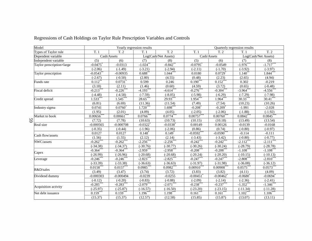
59

Regressions of Cash Holdings on Taylor Rule Prescription Variables and Controls

Model Yearly regression results Quarterly regression results

Types of Taylor rule T. 1 T. 2 T. 1 T. 2 T. 1 T. 2 T. 1 T. 2

Dependent variable Cash/Assets Log(Cash/Net Assets) Cash/Assets Log(Cash/Net Assets)

Independent variable (5) (6) (7) (8) (5) (6) (7) (8)

Taylor prescription×large -0.0475* -0.0313 -1.024** -0.842** -0.0795* -0.0549 -1.976*** -1.717***

(-2.06) (-1.49) (-3.21) (-2.94) (-2.11) (-1.70) (-3.92) (-3.97)

Taylor prescription -0.0543** -0.00935 0.688** 1.044*** 0.0180 0.0729* 1.140** 1.844***

(-2.67) (-0.50) (2.80) (4.55) (0.48) (2.23) (2.65) (4.94)

Funds rate 0.112** 0.0731* 0.599 0.246 0.190*** 0.152*** 0.302 -0.219

(3.18) (2.11) (1.46) (0.60) (4.59) (3.72) (0.65) (-0.48)

Fiscal deficit -0.213*** -0.226*** -4.193*** -4.614*** -0.276*** -0.304*** -3.964*** -4.556***

(-4.48) (-4.58) (-7.59) (-8.05) (-5.98) (-6.29) (-7.29) (-7.98)

Credit spread 1.533*** 1.545*** 28.65*** 29.93*** 1.954*** 1.964*** 30.33*** 30.41***

(6.81) (6.69) (11.36) (11.54) (7.49) (7.54) (10.23) (10.26)

Industry sigma 0.0741 0.0760* 1.720*** 1.698*** -0.208* -0.209* -1.991 -2.028

(1.95) (2.01) (4.09) (4.05) (-2.05) (-2.06) (-1.88) (-1.92)

Market to book 0.00656*** 0.00661*** 0.0766*** 0.0774*** 0.00757*** 0.00760*** 0.0842*** 0.0845***

(7.72) (7.78) (10.63) (10.73) (10.15) (10.18) (13.49) (13.54)

Real size -0.000565 -0.000708 -0.0322* -0.0338* 0.00149 0.00126 -0.0139 -0.0168

(-0.35) (-0.44) (-1.96) (-2.06) (0.86) (0.74) (-0.80) (-0.97)

Cash flow/assets 0.0127 0.0127 0.148* 0.149* -0.0592*** -0.0590*** -0.114 -0.111

(1.56) (1.55) (2.12) (2.14) (-3.43) (-3.42) (-0.80) (-0.77)

NWC/assets -0.262*** -0.262*** -2.256*** -2.256*** -0.242*** -0.242*** -2.112*** -2.111***

(-34.38) (-34.37) (-30.76) (-30.77) (-30.26) (-30.24) (-28.79) (-28.78)

Capex -0.364*** -0.364*** -2.959*** -2.958*** -0.208*** -0.208*** -1.108*** -1.108***

(-26.99) (-26.96) (-20.68) (-20.68) (-20.24) (-20.20) (-10.15) (-10.13)

Leverage -0.246*** -0.246*** -2.823*** -2.825*** -0.247*** -0.247*** -2.808*** -2.810***

(-33.39) (-33.38) (-36.63) (-36.63) (-31.97) (-31.98) (-36.08) (-36.12)

R&D/sales 0.0158*** 0.0157*** 0.0985*** 0.0982*** 0.00910*** 0.00908*** 0.0575*** 0.0573***

(3.49) (3.47) (3.74) (3.72) (3.83) (3.82) (4.11) (4.09)

Dividend dummy -0.000303 -0.000494 -0.0239 -0.0255 -0.00451* -0.00462* -0.0680* -0.0694*

(-0.12) (-0.20) (-0.83) (-0.88) (-2.09) (-2.14) (-2.36) (-2.41)

Acquisition activity -0.285*** -0.283*** -2.079*** -2.071*** -0.238*** -0.237*** -1.352*** -1.346***

(-25.97) (-25.87) (-16.57) (-16.50) (-23.20) (-23.15) (-11.34) (-11.28)

Net debt issuance 0.159*** 0.159*** 1.196*** 1.198*** 0.161*** 0.161*** 1.102*** 1.106***

(15.37) (15.37) (12.57) (12.58) (15.85) (15.87) (13.07) (13.11)

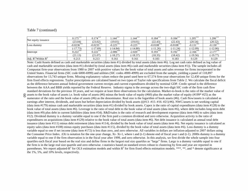
60

Table 7 (continued)

Net equity issuance 0.175*** 0.174*** 1.144*** 1.144*** 0.184*** 0.184*** 1.205*** 1.206***

(23.04) (23.02) (19.01) (19.01) (22.43) (22.43) (20.54) (20.52)

Loss dummy -0.0236*** -0.0235*** -0.225*** -0.225*** -0.0108*** -0.0108*** -0.131*** -0.130***

(-17.73) (-17.69) (-14.84) (-14.80) (-11.26) (-11.24) (-12.09) (-12.06)

Intercept 0.222*** 0.222*** -2.006*** -2.020*** 0.193*** 0.192*** -2.166*** -2.177***

(21.13) (21.07) (-18.27) (-18.37) (18.35) (18.42) (-19.56) (-19.77)

Adj. R2/Within R2 0.213 0.213 0.161 0.161 0.183 0.183 0.129 0.129

Note: Cash/Assets defined as cash and marketable securities (data item #1) divided by total assets (data item #6). Log net cash ratio defined as log value of

cash and marketable securities (data item #1) divided by (total assets (data item #6)-cash and marketable securities (data item #1)). The sample includes all

Compustat firm-year observations from 1980 to 2007 with positive values for the book value of total assets and sales revenue for firms incorporated in the

United States. Financial firms (SIC code 6000-6999) and utilities (SIC codes 4900-4999) are excluded from the sample, yielding a panel of 118,897

observations for 13,743 unique firms. Missing explanatory values reduce the panel used here to 67,574 firm-year observations for 12,430 unique firms for the

firm fixed effects regressions. Taylor prescriptions are calculated based on two types of Taylor rule specifications from Table 2. We calculate the fiscal deficit

as the difference between annual federal government current receipts and current expenditures divided by nominal GDP. Credit spread is the difference

between the AAA and BBB yields reported by the Federal Reserve. Industry sigma is the average across the two-digit SIC code of the firm cash flow

standard deviations for the previous 10 years, and we require at least three observations for the calculation. Market-to-book is the ratio of the market value of

assets to the book value of assets i.e. book value of assets (#6) minus the book value of equity (#60) plus the market value of equity (#199* #25) as the

numerator of the ratio and the book value of assets (#6) as the denominator. Real size is the logarithm of book assets (#6). Cash flow/assets is calculated as

earnings after interest, dividends, and taxes but before depreciation divided by book assets (((#13–#15–#16–#21)/#6). NWC/assets is net working capital

(data item #179) minus cash and marketable securities (data item #1) divided by book assets. Capex is the ratio of capital expenditures (data item #128) to the

book value of total assets (data item #6). Leverage is the ratio of total debt to the book value of total assets (data item #6), where debt includes long-term debt

(data item #9) plus debt in current liabilities (data item #34). R&D/sales is the ratio of research and development expense (data item #46) to sales (data item

#12). Dividend dummy is a dummy variable equal to one if the firm paid a common dividend and zero otherwise. Acquisition activity is the ratio of

expenditures on acquisitions (data item #129) relative to the book value of total assets (data item #6). Net debt issuance is calculated as annual total debt

issuance (data item #111) minus debt retirement (data item #114), divided by the book value of total assets (data item #6). Net equity issuance is calculated as

equity sales (data item #108) minus equity purchases (data item #115), divided by the book value of total assets (data item #6). Loss dummy is a dummy

variable equal to one if net income (data item #172) is less than zero, and zero otherwise. All variables in dollars are inflation-adjusted to 2007 dollars using

the Consumer Price Index. ΔXt is notation for the one-year change, Xt- Xt-1, where t and (t-1) denote end of fiscal year t and (t-1). 2000s dummy is a dummy

variable equal to one if the firm observation is in the fiscal year after 1999, and zero otherwise. In this analysis, we first divide the whole sample into four

quartiles each fiscal year based on the real size and define firms in the largest real size quartiles as “large” firms. Large is a dummy variable equal to one if

the firm is in the large real size quartile and zero otherwise. t-statistics based on standard errors robust to clustering by firm and year are reported in

parentheses. We report adjusted-R2 for OLS estimation models and within R

2 for firm fixed effects estimation models. ***, **, and * denote significance at

the 1%, 5%, and 10% levels, respectively.

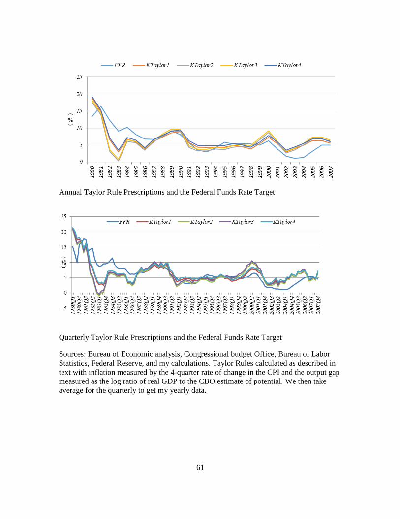
61

Annual Taylor Rule Prescriptions and the Federal Funds Rate Target

Quarterly Taylor Rule Prescriptions and the Federal Funds Rate Target

Sources: Bureau of Economic analysis, Congressional budget Office, Bureau of Labor

Statistics, Federal Reserve, and my calculations. Taylor Rules calculated as described in

text with inflation measured by the 4-quarter rate of change in the CPI and the output gap

measured as the log ratio of real GDP to the CBO estimate of potential. We then take

average for the quarterly to get my yearly data.

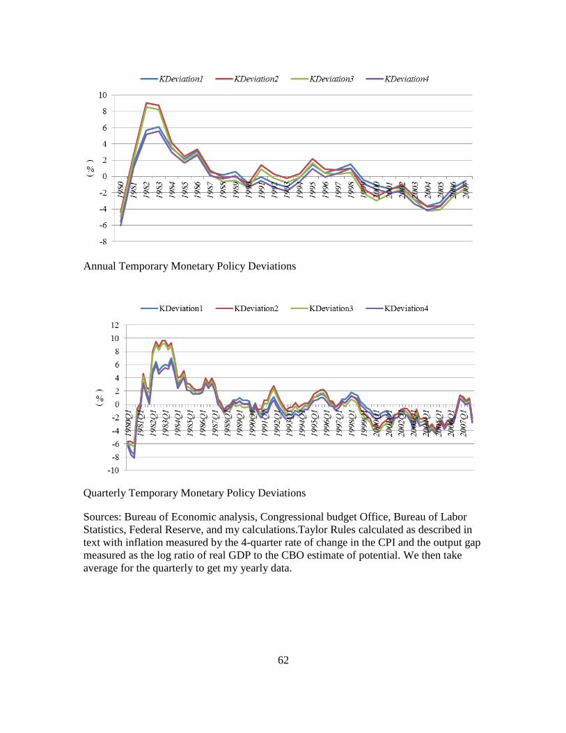
62

Annual Temporary Monetary Policy Deviations

Quarterly Temporary Monetary Policy Deviations

Sources: Bureau of Economic analysis, Congressional budget Office, Bureau of Labor

Statistics, Federal Reserve, and my calculations.Taylor Rules calculated as described in

text with inflation measured by the 4-quarter rate of change in the CPI and the output gap

measured as the log ratio of real GDP to the CBO estimate of potential. We then take

average for the quarterly to get my yearly data.

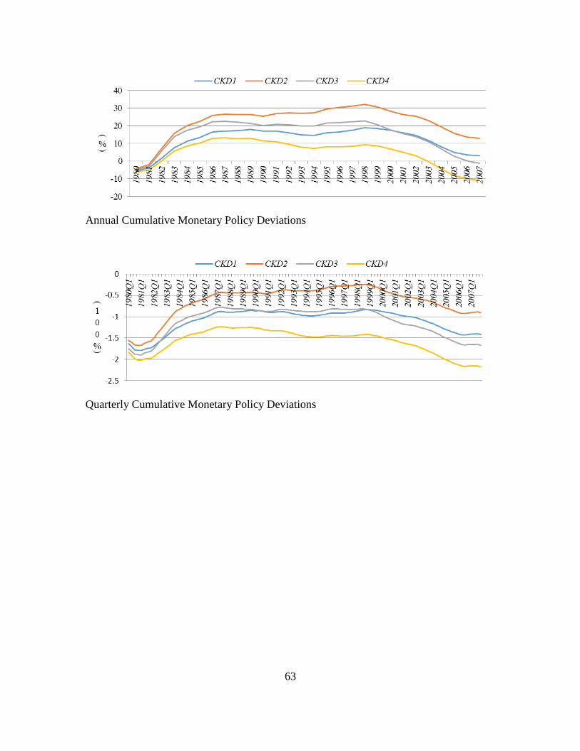
63

Annual Cumulative Monetary Policy Deviations

Quarterly Cumulative Monetary Policy Deviations

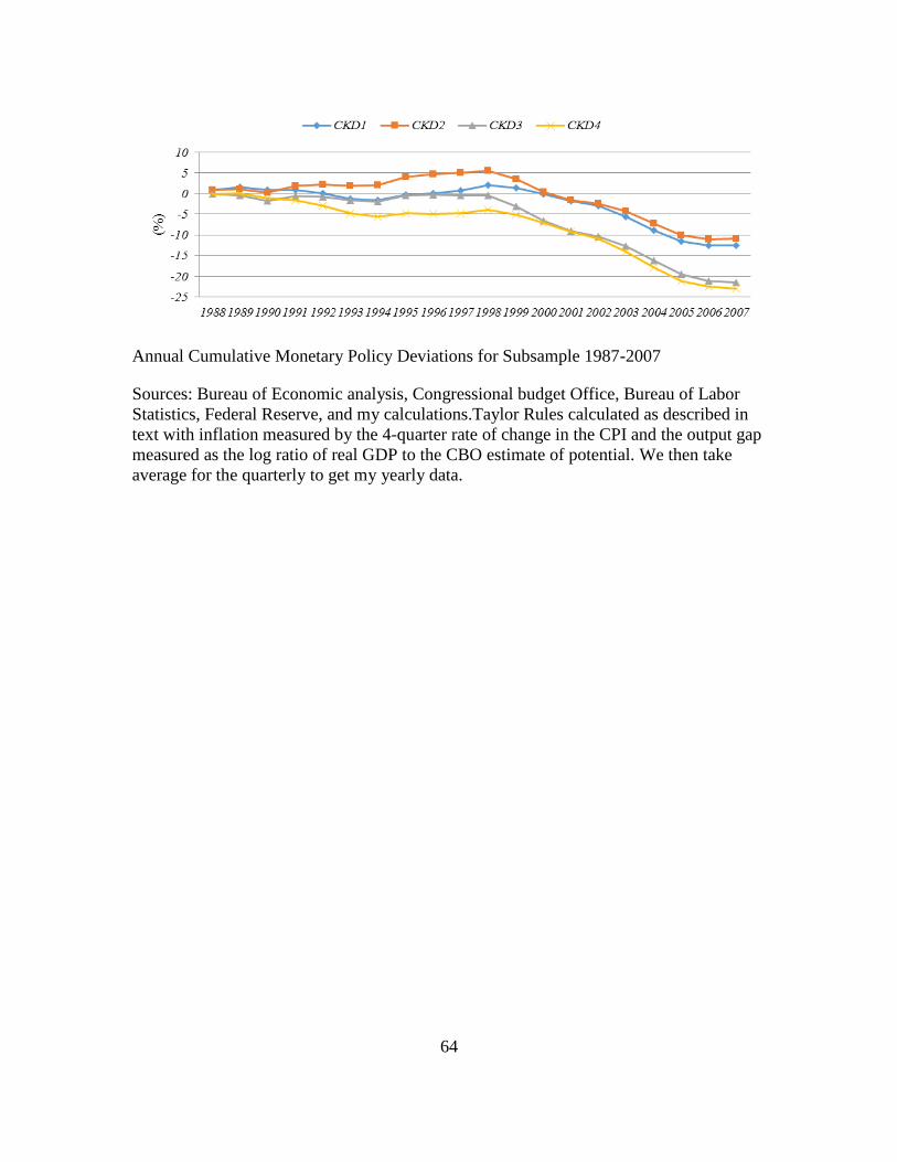
64

Annual Cumulative Monetary Policy Deviations for Subsample 1987-2007

Sources: Bureau of Economic analysis, Congressional budget Office, Bureau of Labor

Statistics, Federal Reserve, and my calculations.Taylor Rules calculated as described in

text with inflation measured by the 4-quarter rate of change in the CPI and the output gap

measured as the log ratio of real GDP to the CBO estimate of potential. We then take

average for the quarterly to get my yearly data.

65

References

[1] Baker, M., & Wurgler, J. (2002). Market Timing and Capital Structure. The Journal of

Finance, 57(1), 1-32.

[2] Bates, T. W., Kahle, K. M., & Stulz, R. M. (2009). Why Do U.S. Firms Hold so Much

More Cash than They Used To?. The Journal of Finance, 64(5), 1985-2021.

[3] Baumol, W. J. (1952). The Transactions Demand for Cash: An Inventory Theoretic

Approach. The Quarterly Journal of Economics, 545-556.

[4] Bernanke, B. S. (2010, January). Monetary Policy and the Housing Bubble. In speech at

the Annual Meeting of the Annual Meeting of the American Economic Association,

Atlanta, Georgia.

[5] Ben, S. B., & Alan, S. B. (1992). The Federal Funds Rate and the Channels of Monetary

Transmission. American Economic Review, 82, 901-921.

[6] Chen, S. S. (2007). Does Monetary Policy Have Asymmetric Effects on Stock

Returns?. Journal of Money, Credit and Banking, 39(2-3), 667-688.

[7] Choe, H., Masulis, R. W., & Nanda, V. (1993). Common Stock Offerings across the

Business Cycle: Theory and Evidence. Journal of Empirical Finance, 1(1), 3-31.

[8] Choi, W. G., & Kim, Y. (2001). Monetary Policy and Corporate Liquid Asset

Demand (Vol. 1). International Monetary Fund.

[9] Choi, W. G., & Kim, Y. (2005). Trade Credit and the Effect of Macro-Financial Shocks:

Evidence from U.S. Panel Data. Journal of Financial and Quantitative Analysis, 40(4),

897.

[10] Christiano, L. J., Eichenbaum, M., & Evans, C. (1996). The Effects of Monetary Policy

Shocks: Evidence from the Flow of Funds. The Review of Economics and Statistics, 16-

34.

[11] Dale, S., & Haldane, A. G. (1995). Interest Rates and the Channels of Monetary

Transmission: Some Sectoral Estimates. European Economic Review, 39(9), 1611-1626.

[12] De Haan, L., & Sterken, E. (2006). The Impact of Monetary Policy on the Financing

Behaviour of Firms in the Euro Area and the UK. European Journal of Finance, 12(5),

401-420.

[13] Fisher, I. (1930). The Theory of Interest. New York, 43.

[14] Fritz Foley, C., Hartzell, J. C., Titman, S., & Twite, G. (2007). Why do Firms Hold so

Much Cash? A Tax-based Explanation. Journal of Financial Economics,86(3), 579-607.

66

[15] Friedman, Milton. Money, Quantity Theory. In International Encyclopedia of the Social

Sciences, pp. 432-47. New York: Macmillan and Free Press, 1968.

[16] Gertler, M., & Gilchrist, S. (1993). The Role of Credit Market Imperfections in the

Monetary Transmission Mechanism: Arguments and Evidence. The Scandinavian

Journal of Economics, 43-64.

[17] Gertler, M., & Gilchrist, S. (1994). Monetary Policy, Business Cycles, and the Behavior

of Small Manufacturing Firms. The Quarterly Journal of Economics,109(2), 309-340.

[18] Hilsenrath, Jon, Easy-Money Era a Long Game for Fed. The Wall Street Journal, page

A2 in the U.S. edition. March 18, 2013.

[19] Hoffman, D. L., & Schlagenhauf, D. E. (1985). Real Interest Rates, Anticipated Inflation,

and Unanticipated Money: A Multi-Country Study. The Review of Economics and

Statistics, 284-296.

[20] J. M. Keynes, The General Theory of Employment, Interest and Money. New York 1936.

[21] Kahn, G. A. (2010). Taylor Rule Deviations and Financial Imbalances. Federal Reserve

Bank of Kansas City Economic Review, Second Quarter, 63-99.

[22] Labonte, Marc. (2013). Federal Reserve: Unconventional Monetary Policy Options,

Congressional Research Service report for congress, R42962.

[23] Meulendyke, A. M. (1998). U.S. Monetary Policy and Financial Markets. New York:

Federal Reserve Bank of New York.

[24] Miller, M. H., & Orr, D. (1966). A Model of the Demand for Money by Firms. The

Quarterly Journal of Economics, 80(3), 413-435.

[25] Mishkin, F. S. (1981). The Real Rate of Interest: An Empirical Investigation, Carnegie-

Rochester Conference Series on Public Policy. The Cost and Consequences of Inflation,

Autumn 1981, 15, 151-200.

[26] Mishkin, F. S. (1996). The Channels of Monetary Transmission: Lessons for Monetary

Policy (No. w5464). National Bureau of Economic Research.

[27] Olivei, G. and Tenreyro, S. (2007), The Timing of Monetary Policy Shocks, American

Economic Review, 97(3), 636-663.

[28] Opler, T., Pinkowitz, L., Stulz, R., & Williamson, R. (1999). The Determinants and

Implications of Corporate Cash Holdings. Journal of Financial Economics,52(1), 3-46.

[29] Pál, R. and Ferrando, A. (2010) Financing constraints and firms' cash policy in the Euro

area. The European Journal of Finance. 6 (2), 153-171

67

[30] Pandey, I. M., & Bhat, R. (2007). Dividend behaviour of Indian companies under

monetary policy restrictions. Managerial Finance, 33(1), 14-25.

[31] Sánchez, J. M., & Yurdagul, E. (2013). Why Are Corporations Holding So Much Cash?

Federal Reserve Bank of St. Louis’ The Regional Economist, 21(1), 5-8.

[32] Stern, G., & Miller, P. (2004). Avoiding Significant Monetary Policy Mistakes. Federal

Reserve Bank of Minneapolis Quarterly Review, 28(2), 2-9.

[33] Taylor, J. B. (1993, December). Discretion Versus Policy Rules in Practice. In Carnegie-

Rochester conference series on public policy (Vol. 39, pp. 195-214). North-Holland.

[34] Taylor, J. B. (1998). A Historical Analysis of Monetary Policy Rules, National Bureau of

Economic Research conference on Monetary Policy Rules.

[35] Taylor, J. B. (1999). The Robustness and Efficiency of Monetary Policy Rules as

Guidelines for Interest Rate Setting by the European Central Bank. Journal of Monetary

Economics, 43(3), 655-679.

[36] Taylor, J. B. (2007). Housing and Monetary Policy (No. w13682). National Bureau of

Economic Research.

[37] Tobin, James, (1956), The Interest Elasticity of the Transactions Demand for

Cash, Review of Economics and Statistics, August, vol. 38, no. 3, pp. 241–247.

[38] Zaman, A. A. (2011). Cash Holdings, Market Frictions and Monetary Policy: An

Investigation of Increase in Cash Holdings. Market Frictions and Monetary Policy: An

Investigation of Increase in Cash Holdings (June 4,2011).