core.ac.uk · the dynamics of lateral bending and torsion vibration of a ... excitation and...

LATERAL VIBRATION OF THIN BEAMUNDER VERTICAL EXCITATION

by

VIVEKANANDA MUKHOPADHYAYB. Tech., Indian Institue of Technology, Kharagpur

(1968)

SUBMITTED IN PARTIAL FULFILLMENTOF THE REQUIREMENTS FOR THEDEGREE OF MASTER OF SCIENCE

at' theMASSACHUSETTS INSTITUTE OF TECHNOLOGY

June 1970

Signature of Author ----~---Department of Aeronauticsand Astronautics, June 6, 1970

Certified by

Thesis Supervisor

Accepted by ...-- ----

LATERAL VIBRATION OF THIN BEAMUNDER VERTICAL EXCITATION

byVivekananda Mukhopadhyay

Submitted to the Department of Aeronautics and Astronauticson June 6, 1970 in partial fulfillment of the requirements forthe degree of Master of Science.

ABSTRACTThe dynamics of lateral bending and torsion vibration of a

thin flexible beam under vertical harmonic excitation has beeninvestigated theoretically and experimentally. Only lineartheory is considered for theoretical analysis.

The governing equations are a set of coupled Mathieu typeequations. Initial built-in deflections introduce forcingterms resulting in coexistence of parametric and forced excita-tion. The instability regions and steady state solutions arestudied here.

Experimentally, the beam was excited and transient andsteady state records were obtained. Three regions of instabilitywere observed, only one of which is a linear phenomenon andagrees well with the theoretical results. The other two regionshave large bending and torsion amplitudes and exhibit limitcycle type behavior. Also, peculiar snapping and whippingmotions were observed. An elaborate nonlinear analysis isrequired to explain the later experimental results which arepresented in detail.

Thesis Supervisor: John DugundjiTitle: Associate Professor of

Aeronautics and Astronautics

iii

ACKNOWLEDGEMENTS

The author wishes to acknowledge with gratitude the timeand effort devoted by Professor John Dugundji who suggested theproblem, provided continuous guidance and spent long hourshelping in the experiment.

Sincere appreciation is extended to the Department ofAeronautics and Astronautics of MIT for the research assistant-ship.

The author is also indebted to his parents for their con-tinuous encouragement throughout his study.

Finally, thanks are due to Messrs. F. Merlis, A. Shaw,J. Barley, O. Wallin for helping set up the experiment and toMiss M. Bryant for her excellent typing.

iv

TABLE OF CONTENTS

Chapter

1

2

3

4

INTRODUCTIONTHEORETICAL ANALYSIS2.1 Mathematical Formulation2.2 Pure Parametric Excitation

a) First Instability Regionb) Second Instability Region

2.3 Forced Excitation2.4 Forced Excitation (Two Mode

Approximation)EXPERIMENTAL INVESTIGATION3.1 Test Setup3.2 Test Procedure3.3 Discussion of Experimental ResultsCONCLUSIONS

1

4

4

10121619

22262627

28

33

AppendicesA

B

MODE SHAPESEVALUATION OF CONSTANT TERMS

36

31REFERENCESTABLESFIGURES

414241

v

LIST OF SYMBOLS

aI' a2AI' Bl, BOI

Dimensionless frequency parameters (Eq. 2.15)

Coefficients of assumed solutions (Eq. 2.20and 2.23)

Constants defined in Eq. (B.l)

Coefficients of assumed solutions (Eq. 2.26)

Thickness of the beam

Dimensionless built-in bending amplitude

Matrices defined in Eq. (2.21) and (2.24)

Modal damping coefficients

Width of the beam

Constant defined in Eq. (B.l)

Modulus of elasticity

Dimensionless self weight (Eq. 2.15)

static bending amplitude (Eq. B.2)If

A2, B2, B02Aa, Ba, BOa

AI' Bl, BOIA2, B2, B02Aa, Ba, BOa.b

BBBS

AI' Bl, ClA2, B2, C2CSl' CS2[Cl]' [C2]

CVl' CV2' Ced

D

E

Fl

vi

Defined in Eq. (2.15)

Dimensionless static buckling self-weight

Acceleration due to gravity

Shear modulus

Constant defined in Eq. (B.1)

Dimensionless bending mode shapes*h1(n), h2(n)

hD(n,t)

hS(n)

H

""

dynamic bending deflection

static equilibrium position

I

m

MXO' MyO MZO,MX' My, MZP(s)

Area moment about Z axis

Mass-rotary inertia about X axis

Polar area-moment about X axis

Dimensionless constant (Eq. 2.15)

Length of the beam

Mass per unit length

External moments about Xo' Yo' Zo axes

" " "X, y, Z axes

Distributed vertical load


Dimensionless generalized coordinates*II

2.15)torsion natural frequency (Eq.

vii

Time in seconds

Dimensionless built-in twist amplitude


Length coordinate along the beam

Constant defined in Eq. (B.l)


Amplitude of base motion in inches

Dimensionless amplitude of base motion


Total bending deflection

Built-in bending deflection

Dynamic bending deflection

Static bending equilibrium position

Value of VD at tip of the beam

Forcing frequency

Bending mode natural frequencies.

First torsion mode natural frequency

Length coordinate along Xo axis

undeformed axes system

Deformed axes system

static twist amplitude (Eq. B.2)"

TBTSUBUIBU2BV(s,t)

VB(s)

VD(s,t)

VS(s)

VTWFWlh, W2hWa.

x

Xo' Yo' Z0

X, Y, Z

s

~l' t2, ta

6(s,t)

6B(s)

6D(s,t)

6S(s)

6Tn

a

T

(.)(0)

({( ) t

viii


First torsion mode shape

Modal critical damping ratios*

Total torsion in radians

Built-in twist in radians

Dynamic torsional deflection in radians

static torsion equilibrium position in radians

Value of 6D at tip of the beam

Dimensionless length coordinate = s/1

Complex constant (Eq. 2.20 and 2.23)

Dimensionless time = (WF/2)t

Dummy variable of integration

Time derivative

Dimensionless time derivativeDerivative w.r.t. sDerivative w.r.t. n

* 1, 2 and a refers to 1st bending, 2nd bending and 1st torsionmodes respectively.

CHAPTER 1

INTRODUCTION

Parametric excitation, characterized by the variation ofa parameter in an equation has been well known and was studiedin detail by many authors. Bolotinl has investigated theapplication of parametric excitation to structural systems.

The physical nature of parametric excitation and of morefamiliar forced excitation may be distinguished by the factsthat (1) for linear, low damped systems, the parametricoscillations occur over a continuous range of forcing frequen-cies of the varying parameter, where as the forced oscillationshave the resonance behavior only at discrete values of theforcing frequency, and (2) for a simple pendulum and for aflexible beam, the parametric oscillations occur in the direc-tion normal to the excitation, while the forced oscillationstake place in the direction of the excitation. Both parametricand forced excitation can exist together in a system. Asimple pendulum whose pivot point is oscillated along a linewhich is tilted at an angle to the vertical, receives bothkinds of excitation. Linear and nonlinear analysis of suchphenomena has been done in detail for both pure parametricexcitation and combined parametric-forced excitation byDugundji and Chhatpar2,3 and provides a background for thepresent study.

2

A thin flexible cantilever beam whose base is oscillatedvertically in the plane of the web which is also the plane oflargest rigidity, experiences a periodic load which appearsas a parametric term in the out-of-plane bending-torsionequilibrium equation. In the static case, the considerationof small lateral deflection under vertical load leads to thestatic stability problem. Analogous to the pendulum problem,if the beam has an initial static deflection due to built-inimperfections or if the web is initially tilted from vertical,forcing functions appear in the dynamic equilibrium equationsand both parametric and forced excitation occur simultaneously.After applying Galerkin's technique with assumed normal modeshapes as weighting functions, a set of coupled equations areobtained for the time domain analysis. These equations havethe same characteristics as the Mathieu equation and have beenanalyzed in detail by Bolotinl but no experimental results arepresented. The present report investigates the problem oflateral vibration of thin beam both theoretically and exper-imentally. Only the linear theory for small motion is con-sidered and presented in Chapter 2. The experimental investiga-tion is presented in Chapter 3. A representative experimentalobservation is tabulated in Table 2. Three regions ofinstability were observed only one of which is a linearphenomenon and agrees well with theoretical results and isdescribed at the end of Chapter 2. The other two regions havelarge bending and torsion amplitudes and exhibit limit cycle

3type behavior. Also peculiar snapping and whipping motionsare observed. An elaborate nonlinear analysis is required toexplain the later experimental results which are presented indetail. Bolotinl briefly discusses the nonlinear problem butthe solution is inadequate to explain them. The nonlinearitiesare not quite well defined and further work is required inthis direction.

4

CHAPTER 2

THEORETICAL ANALYSIS

2.1 Mathematical FormulationThe beam shown in Fig. 4, which has an initial built-in

deflection and twist VB' aB with no stress developed, assumesa position Vs' as after static deflection under self-weight.The final state V, a indicates position due to dynamic loadingat any instant of time. All external forces P(s) are acting inZo direction. Thus moments acting in Xo' Yo' Zo directions ata distance s from the root on the beam neutral axis are

~Mxo == f PU:o[ V(~) - yes) J J~

..5

Myo = tpes) [ :>t (~) - Xes)} cl~5

(2.1)Mzo - 0

in a right-hand system where V(s) is the position coordinateof the neutral axis in the Yo direction, X(s) is the coordinatein Xo direction of the point s under consideration and i is thelength of the beam. Resolving the moments in the deformeddirection XYZ (Fig. 4) one gets under small deflection assump-tion

5

Mx = M)(o + oV M05 yo

M M-yo ?:;V + 8Mzoy = "'C)5 Mxo(2.2)

M~ = M;lO eMyo

where e is the total twist about neutral X axis measured fromvertical direction in the right hand system. Since the beam isconsidered infinitely rigid in Z direction compared to Y direc-tion because of its shape, the deflection in Z direction havebeen neglected in such a vector transformation. Since onlythe linear equations will be formulated here one can writex : s and take deflections in the deformed direction same as inthe undeformed direction. Thus using the engineering bendingand St. Venant torsion theory neglecting warping the staticmoment equilibrium equations in Z and X directions become

- Mz

GJ d (e - ee)dS (2.4)

where EI is the flexural stiffness about Z axis and GJ is thetorsional stiffness about X axis.

To obtain the force equilibrium equations for the dynamicproblem, one differentiates Eq. (2.3) twice and Eq. (2.4) oncewith respect to s and introduces inertia and damping terms

6

appropriately. If the base of the beam is given an accelera-tion UB in Zo direction, the loading term pes) becomes

(2.5)where m is mass per unit length, g is acceleration due to

it d (.) - th ti d i t- a() Th th d igrav Y an lS e me er va lve ar-. us e ynam cforce equilibrium equations can be written as

(2.6)

where 1m is the rotary moment of inertia per unit length aboutX axis, Cv and Ce are bending and torsion damping coefficientsrespectively. The ( )1 represent ~~). By definitionV = VD+VS' 8 = 8D+8S' where Vs and as represent the staticequilibrium position coordinates; VD and 8D are the deflectionand twist measured from the static equilibrium position.SUbtracting the static equilibrium equations

= 0 (2.8)

(2.9)

7

from Eq. (2.6) and (2.7) the following equations are obtained.'?J4V ~ /1.. II

EI dS4D - ~(~-GB)l(t-5) eD1 + m~6 [(t-:»2Ss]

+ -mVD + (v V'D = 0(2.10)

.. .- Im8:o - (8 8]) = 0

(2.11)

Nondimensionalizing by writing n = 5/1, hn = Vn/1, h~ = VS/1

after rearrangement

I CV,A._ +n1) + m n1>

(2.11)

•.. + Ce eDej)1m

- a()where ()t - all.

(2.12)

8

We introduce2-

h1) (~, t) - 2: hn(1) ~n(t)YL= I (2.13)

en (1, t) = 0:(1) {cx(t)

where the assumed mode shapes hn(n), a(n) satisfy all boundaryconditions (Appendix A). We take only the first torsion modeand first and second bending modes since they are the onlydominant modes encountered in the experiment. ApplyingGa1erkin's technique namely multiplying Eq. (2.11) by h1(n) andh2(n) successively and Eq. (2.12) by a(n) and integrating w.r.t.n from a to 1 we get the modal equations

(2.14a)

(2.14b)

(2.14c)

The new symbols A1, B1, C1, H, D, etc. are constants and are

9

defined in the Appendix B. Also because of orthogonality of(I I " II

the assumed mode shapes Jo

11.1-Jz d'1. = 0 10 {, 1 -h2 d1 :=. 0 ;

consequently there is no coupling between q1 and q2 in Eq.(2.14a) and (2.14b)~ if one uses modal damping coefficients.Denoting

2{U2.h

U28

(2.15)

10

and introducing

2c:.

(2.16)

(2.17)

for harmonic base motion with amplitude UB and forcingfrequency WF and nondimensional time L we get the equationsin their final form00 0

~I +2~,jQ\~1 +QI~, -[o.,F, +2U\e.Co~2.Llq.a:

= 2U\B Ts (os 2 L00 0

etz + 2 ~2.rq; <;f2 + Qz e;t 2 - [02.fZ + 2 UZf3(as n] <:fa== 2 Uze, Ts Co~ 2"(

00 0

9-a: + 2 ~aJQ(~, ~a + Qir,~a - k( [01 VI + 2Utl~1Con 2t11.

(2.18a)

(2.18b)

where (0) = ~() and we have introduced the values A1=A2=1.One can write a2r2 in place of a1r1 since they both denote('2W /WF) 2 •

a

2.2 Pure Parametric ExcitationIf the right hand side forcing terms originating from

initial static deflection are set equal to zero, we get a set

11

of coupled equations which are similar in characteristics tothe well known Mathieu Equationsl, and can be treated in asimilar fashion. However, because of their complexity, it isnot possible to write closed form approximate solutions.However, we shall demonstrate here how one proceeds to deter-mine the solutions.and the instability regions, when the twobending modes and one torsion mode are participating.

By going into the general theory discussed by Bolotinl, itcan be shown that certain values of WF and UB lead to unbounded,i.e., unstable solutions while other values lead to bounded orstable solutions. A plot of-WF versus UB can then be constructedseparating the stable and unstable regions of these equations.Such plots are shown in Fig. 5 and 6 in WF/2Wlh vs. UIB. Forsmall values of UlB, U2B various regions of instability developnear al : 1, 4, 9, •• a2: I, 4, 9... alrl: 1, 4, 9 ••• etc.

It is observed that near the second instability region ataI' a2,a1rl : 4, i.e. WF : Wlh, W2h, Wa respectively, thereis greatest interaction between the forced and parametricexcitation3 and we obtained this in the experiment. Also forthis investigation IUlBI, IU2BI < 1.The homogeneous equations are

00

<:}, + 2 ~fcil91+ Q\ <;} I - ( Q, F, + 2 U If/CO:; n:11« = a

00

<12 + 2~.J02<;}2 + <l.?~z- [ Q2fl + 2 UolE> Co'S 2t19 a - a

(2.l9a)

(2.l9b)

1200

9-a+2\a:ja.,Y'\9-a + Q'V"I~a - k,[u,F. + 2U,B(os2r]CJI

(2.l9c)

(2.20)CJ2 -

a) First Instability RegionIn the vicinity of first instability region and for

values lulBI, lu2BI < 0.6 a good approximation to the solutionof Eqs. (2.19) can be shown to be2

(f-c'}, e (I) I (Os l + A \ Sin L )

(JL' -e (52 CoSL

where a is a constant to be determined, and AI' Bl etc. areconstants. Substituting Eqs. (2.20) into (2.19) and equatingto zero the coefficients of eO t: sin L, eO C cos't:, and discard-ing eOC sin 3l: , eO?:,cos 3'C terms for this approximation, wehave a set of the following equations.

[ C, ]61

I [l \] B23x'3 3~3 Ba:------+- a (2.21)

I A\-[II] [ 51] A2-

.3X3 I 3x3 Aa.

where

13

0-2+ 2 <),J(il a- D -(a, F, + U'B)

+Q,-\

[e, ] =0 (J '- + 2 S"2. .[Q20- - (Q,2.F2 + U.z 8)

+Qz-l

- k::,(a,f,-+ U\l~) -KI(a2fi +U2&) 2cr +2S"a~Q.lrlcr

+QCY-l- t

'2.(- Qc F, -to U,B )(J 4- 2 S-1J(ic 0- 0

+Q,-l

2

[SI] = 0 cr + 2~.fQ;. cr (-0.2 Fz -+ UZB)-t 0.2 -I

K1(-alf, -t UIB) K,(-Q.2f2+ Uze) <r2.+2 );xl 0.,Y"'l 0-

f Q,'f, - ,

o

o

o

o

o

o

14

For a nontrivial solution of Eq. (2.21), the determinant ~=O.It can be shown that under slowly varying amplitude assumptiona good approximation to Eq. (2.21) may be obtained by neglect-

2ing the 0 and 0 terms in the main diagonal elements of the[el] and [81] matrix. Only the smallest roots of 0 of theresulting determinant are applicable near the instabilityregions. The other roots are sensitive to the neglect ofsin 3C , cos 3C terms. These three values constitute thethree independent solutions of the form of Eqs. (2.20). Iffarther for a particular conbination of WF and UB the real partof the root is positive, it gives an unbounded solution andthe point WF, UB, for given values of ~l' ~2' ~a is unstable.If the real part is negative, the two solutions are boundedand the point WF, UB is stable. The points where the real partof 0 is zero define the boundary between the stable and unstableregions. To complete solution of homogeneous set of equationsEq. (2.19) one evaluates Bl,B2,Ba,A2,Aa in terms of Al afterthe three values of 0 has been found. Then placing these inEq. (2.20) one obtains three independent solutions of ql' q2'and qa corresponding to the three values of o. The twoarbitrary constants for each equation can then be obtained fromthe six initial conditions. One can obtain the stabilityboundary by putting 0=0 in the determinant of coefficients inEq. (2.21). For no damping case, the determinant decouples togive two equations.

15

2 2 }(a.,-I)(Q2-l)(U1yt-l) - kl\C 0., F,-t UI8)( a2.-I) + (D.2F2 + U2.8) (a..-I) = 0

(0.,-1)( Q2-1) (a., Y,-I)- K1{(-alft -I- \)16f(Q2-1) +f-az.F2 +U2.B)2(G,-I) } = 0

(2.22)

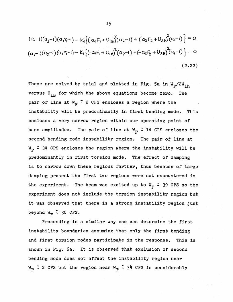
These are solved by trial and plotted in Fig. 5a in WF/2Wlhversus UIB for which the above equations become zero. Thepair of line at WF : 2 CPS encloses a region where theinstability will be predominantly in first bending mode. Thisencloses a very narrow region within our operating point ofbase amplitudes. The pair of line at WF : 14 CPS encloses thesecond bending mode instability region. The pair of line atWF : 34 CPS encloses the region where the instability will bepredominantly in first torsion mode. The effect of dampingis to narrow down these regions farther, thus because of largedamping present the first two regions were not encountered inthe experiment. The beam was excited up to WF : 30 CPS so theexperiment does not include the torsion instability region butit was observed that there is a strong instability region justbeyond WF : 30 CPS.

Proceeding in a similar way one can determine the firstinstability boundaries assuming that only the first bendingand first torsion modes participate in the response. This isshown in Fig. 6a. It is observed that exclusion of secondbending mode does not affect the instability region nearWF : 2 CPS but the region near WF : 34 CPS is considerably

16

narrow. Thus in the first instability region the second bend-ing mode plays a dominant part.

b) .Second Instability RegionIn this region for IU1Bllu2BI < 1 a good approximation

to the solution of Eqs. (2.19) can be shown to be3

err: -il - e (501 + B, Cos 2[ + A,5in2[ )

~2 ::::ere:.e ( 502 + &2 Cas 2"( + A2 5iY12C)

(2.23)

qa: =(rL:, _

Aoc Si-"ZC)e (f:>oGt + Ba Cas 2C +

where 0 is a constant to be determined and B01,Bl etc. areconstants. One may proceed in exactly the same way as for thefirst instability region, i.e. substitute Eqs. (2.23) inEqs. (2.19) and equate to zero the coefficients eO~ , eO~ sin 2~

ot:. or 4 o-r:, e cos 2L , discarding e sin 1:, e cos 4 ~ termsfor this approximation, and proceed to determine 0 for anontrivial solution.

To determine the stability boundary between the divergentand convergent solution, one may proceed with 0=0 to get

where

17

T Bo\

[ C2] [ l2] 502-

Boaf,x, bX~ "5, (2.24)- - - + - - - -- B2. - 0

- [Zz] : [ 52]Bcx.A,

3X~ ~X'3 AzI Arx

Q. 0 - Q,F, 0 0 -U1B

0 a..2 -Q2F2 0 0 -U2B

-K,o.lF; -kla2~ a.,Yj -K,U\!~ - K.,U2B 0

[C2 ]=0 0 -2U1B (Q,-4) a -Q,F,

0 0 -2U2B 0 ( 0.2.-4) -Q2F"l

-2K,U'B -2~IU2B a -K,U,F, -K,<l.2 fi (G..Yj-4)

(O-t-4 ) a -a,F.

o

[lz] =o

o

o

o

o

o

18

o

o

o

o

o

o

o

o

o

For nontrivial solution, the determinant of the coefficientsin Eq. (2.24) must be zero. The combination of WF, UB whichmakes it zero can then be plotted to give the stabilityboundary for given ~1' ~2' ~a. For no damping case, thisdeterminant decoup1es to give two equations

(2.25)

19

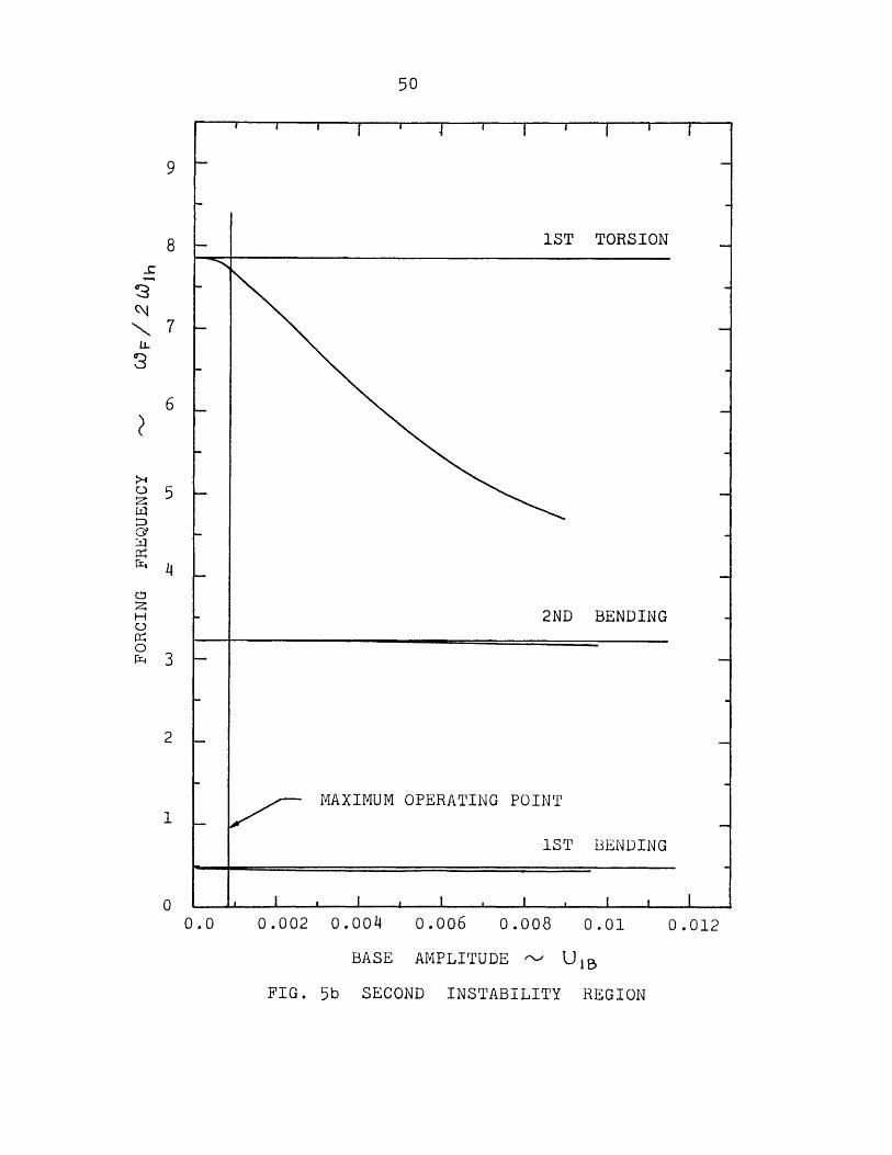
These are solved by trial and plotted in Fig. 5b. in WF/2Wlhversus U1E for which the above equations become zero. Thesecond instability boundaries enclose three regions at WF nearthe natural frequencies of the three modes considered here.The pairs of line at WF : 1 and 7 CPS enclose the regions wherethe instability will be predominantly in the first and secondbending mode respectively. These enclose very narrow regions,and only a mild effect of the region at WF : 7 CPS is observedat higher base amplitudes. The pair of line at WF : 17 CPSencloses a very wide region where the instability will bepredominantly in the first torsion mode. This region isencountered in the experiment.

Proceeding in a similar way one can determine the secondinstability boundaries assuming that only the first bendingand first torsion modes participate in the response. This isshown in Fig. 6b. It is observed that the exclusion;of'~secbridbending mode does not change the instability regions nearWF : 1 and 11 CPS.appreciably. Thus in the second instabilityregion, the second bending mode does not playa dominant part andone can investigate by taking only the first bending and firsttorsion mode.

2.3 Forced ExcitationHere a particular solution of Eqs. 2.18 is desired. A

particular solution is assumed of the form

20

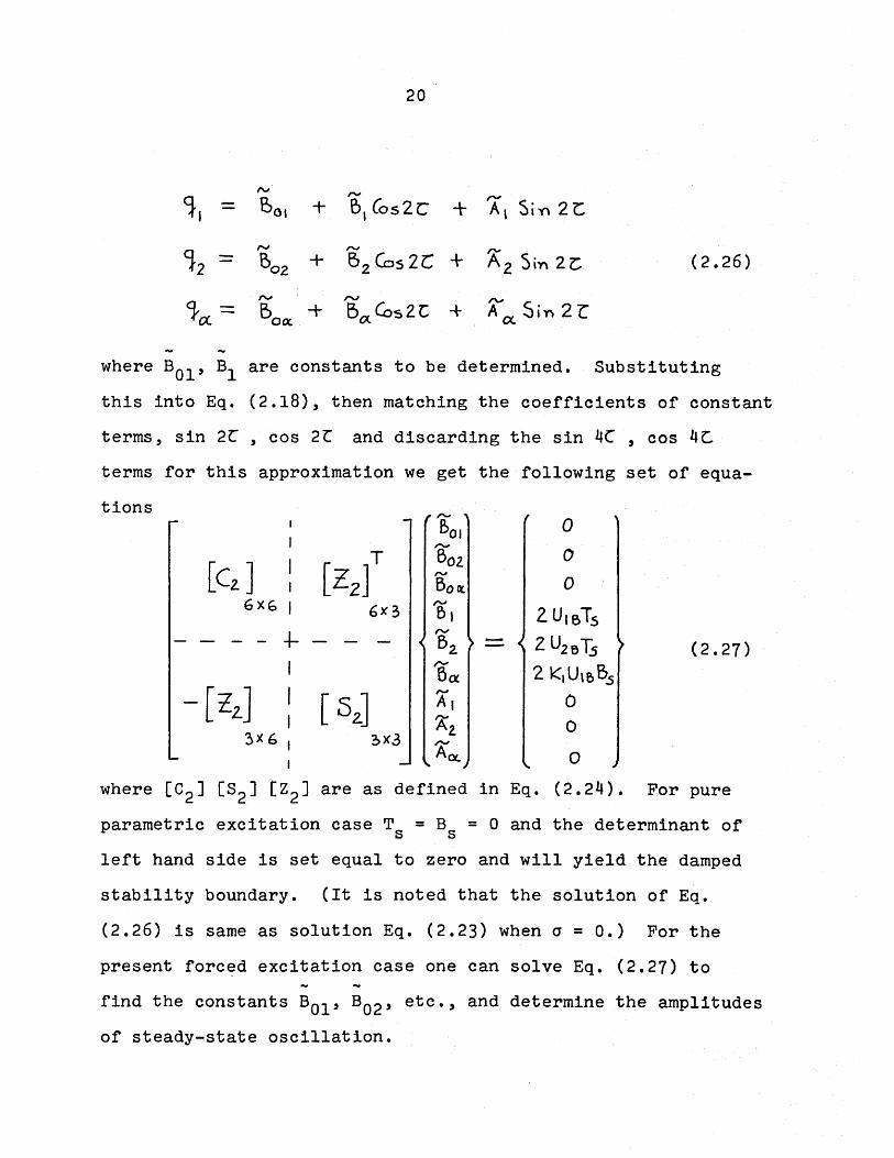
IV ,...,~, ,...,- Bo, + 5, (os2C + A, Si", 2t:

'12 =f'J ,..., ~B02 + 52 Cas 2C + A 2 Sin 2 z: (2.26)rv r-.J

A(X. Sin 2 LC}C( = 500c + BO( Cos 2. t: -+

where B01' Bl are constants to be determined. Substitutingthis into Eq. (2.18), then matching the coefficients of constantterms, sin 2L , cos 2C and discarding the sin 4C , cos 4~terms for this approximation we get the following set of equa-

(2.27)

tions r-

BOI,...,

[(2. ] T Bot[ZzJ /"oJ

Bott6xG 6)(3

,...,BI

+- ,...,- - B2. -

I 'eo:- [l2J I [ 52-J

/"oJ

AII Az3X6 2>)(3 AOL

ooo

2. VI BTsZ U26 Ts2 K,U\e>Bs

ooo

where [C2] [32] [Z2] are as defined in Eq. (2.24). For pureparametric excitation case T = B = 0 and the determinant ofs sleft hand side is set equal to zero and will yield the dampedstability boundary. (It is noted that the solution of Eq.(2.26) is same as solution Eq. (2.23) when a = 0.) For thepresent forc~d excitation case one can solve Eq. (2.27) tofind the constants B01' B02' etc., and determine the amplitudesof steady-state oscillation.

21

The characteristics of the steady state soltution forsmall damping are apparent from the Eq. (2.26) and (2.27).The solution oscillates at the forcing frequency WF• There

... ... ...is a constant center shift BOl,B02,BOa. The coefficients B'sbecome large near the lower bounds of the instability regionsand the coefficients A's dominate the amplitude of oscillationnear the upper bounds in the immediate vacinity of aI' a2,alrl : 4. The amplitudes become infinite at the stabilityboundaries since the determinant of coefficients is zero there.Thus infinite amplitudes appear over a finite frequency gap.However, as the damping ~l l;2~a increases, the gap narrowsand if they are high enough, the infinite amplitudes disappear.

For no damping case, [C2] and [32] decouple and one hasto solve

~ 0BOIrv

B02 0rv

[ C2] Bocx 0t, 2.U1BTs

6Xb rvZ U2.5TS52.

~ 2 K,U1f>BSoc

(2.28a)and

0

[ Sz] 03)(3 0

(2.28b)

22

to determine the amplitude of steady state oscillations. Thecontribution of A1, A2, Aa, will be zero except on the upperbounds of the second instability regions of Fig. 5b wheredeterminant of [S2J is itself zero. The solutions of Eq.(2.28a) are not valid inside the instability regions since thehomogeneous solution is divergent there. Eq. (2.28a) issolved numerically and plotted in Fig. 5c over the frequencyranges of interest for a fixed base amplitude. The constantcenter shifts B01' B02' BOa are of order 10-2 except near theinstability regions.

2.4 Forced Excitation (Two Mode Approximation)In Cha~ter 2.2 it was observed that the second"stabi1ity

regions at WF : 1 and 17 CPS do not change appreciably if thesecond bending mode is excluded. Thus working with just twoequations a closed form steady-state solution can be obtainedwhich includes the damping and the experimental results can becompared. For this case, the particular solution of Eqs.(2.18a) and (2.18c) with q2 set equal to zero is desired.This is easily obtained by contraction of Eq. (2.27) by settingB02 ' B2 and A2 equal to zero and neglecting associated equationsto give

23

r'!!'

Q..l - ad:'; 0 -UlB 0 0 B61 0

-1e,Q.1 Fj Q,r, 0 0,....,

-k,U,e, 0 Boo 0

0 I ~~I.fQ,I'V

-lUH~~ (0.,-4) -Q(F, 0 B, 2 U,&T.s-, -a -k,n,F, (U\f,-4) 0/'V

-2K,UI& 4~alQ,li E>a ZKU'B~+0 0 -4l),fU. 0 I (uc-4) -a,F, AI 0

0 0 0 -4~~' -KiQ,1) (Q.'!i-4) Aa 0,

(2.29)

For pure parametric excitation case, Ts = Bs = 0, thedeterminant of left hand side is set equal to zero and willyield the damped stability boundary. For the present forcedexcitation case, Eq. (2.29) can be solved for B01,Bl, AI' BOa'Ba, Aa to give

24

where

P7 - -ZU1BP' + Q,(F\;-F/")PZ/U1B

P8 - P6 ( : ~I - P5) - P7 FI (PZ - P3)

~S - Jllt/k,(2.30)

25

The characteristics of this steady state solution is same asdiscussed in Chapt~r' 2.3. The solution oscillates at theforcing frequency WF• There is a constant center shift BOIBOa. If the damping is sUfficiently small infinite amplitudewill a~pear over a finite frequency gap. Figure 20 shows thesteady state response amplitude VT/i = 2/A2 + B2 (since

1 1h1(1) = 2) and aT = 'A2 + 82 where VT and aT are bending and

a atorsion tip amplitudes in inches and radians respectively,plotted against forcing frequency WF for the damping case.The damping coefficients are obtained experimentally and hasbeen shown in Figs. 10 and 11. Since they vary with amplitude,an iterative scheme is used to determine the final amplitudewithin "0.005 V~/i and 0.005 radians, accuracy. VT/i are oforder 10-3 and has not been plotted. The constant terms inthe assumed solution are of order 10-2• Figure 20 also showsthe experimental points. It is seen that the linear theorygives a fairly good estimate of the torsion amplitudes for WFless than 17 CPS, considering that, the error involved in theforcing frequency measurement is of order 0.1 CPS. It may benoted that the sharp drop in torsion amplitude near WF - 17CPS for all amplitudes of base motion is due to the fact thatthe upper instability boundary is independent of the baseamplitude UB (Fig. 5b).

26

CHAPTER 3

EXPERIMENTAL INVESTIGATION

3.1 Test SetupThe setup for the experimental observation of lateral

vibration behavior of flexible beam under vertical excitationis shown in Figs. 1 and 2. The schematic sketch is given inFig. 3. The test specimen chosen is a 0.02 in. thick 3.0 in.wide AL 6061-T6 beam, clamped at one end to form a 24.0 in.cantilever. The base is mounted rigidly to the shake-tablesuch that the web of the beam is vertical. The shake-tableoscillates vertically and generates a harmonic excitation overa frequency range from 2 to 50 CPS. The frequency of theshake-table is measured by using a strain gage mounted on athin bar which is bolted to the shake-table at one end andfixed at the other.

The bending frequency and amplitude are derived from thesignal from two strain gages mounted on each side of the beamnear the root along the longitudinal principal axis. Thesestrain gages do not respond to twisting about that axis, andform two arms,'ofthe balancing bridge. This eliminatestemperature error. The torsion amplitude and frequency arederived from the four strain gages, two of which are mountedsymmetrically at 45° about the longitudinal axis. The othertwo are placed alike directly on the other side of the beam.

21

They act as four arms of the bridge as shown in Fig. 3. Thetorsion strain gages pickup some signal when the beam is bend-ing but this does not show up in the recordings when thetwisting frequency is different from the bending frequency.The signal picked up by the torsion gage for pure static bend-ing is shown in Fig. 1.

3.2 Test ProcedureThe beam is clamped so that its web is vertical near the

root with respect to the horizontal shake-table. It isobserved that the beam because of its flexibility and initialimperfections leans slightly to the negative Yo direction.The tip static deflection is estimated to be 0.25 inches. Thebending and torsion response of the beam is investigated overthe forcing frequency range from 2 to 30 CPS for four differentbase amplitudes of 0.0125, 0.025, 0.0315 arid0.050 inches.The strain gages are first calibrated for static deflectionand twist due to a point load and torque at the tip. Thestrain gages are then calibrated uynamica11y by exciting thebeam at different measurable tip amplitudes in first, second,and third bending mode and in first twisting mode. These areshown in Figs. 8 and 9. The static calibration which could bedone only for first bending and first torsion are also shownafter zero correction. Only the dynamic calibration is usedfor conversion.

To estimate the damping ratio, dynamic decay record istaken for first and second bending and first torsion. Some

28

typical records 'are :shown in !Flgs. 12 arid13. The torsionchannel of Fig. 12 shows how the torsion gages picks up bend-ing. From bending channel of Fig. 13, it is apparent that thebending gages do not pickup appreciable torsion. The dampingratios are determined from the slope of the decay recordsplotted on sami-log papers. The variations of damping ratiowith amplitude are shown in Figs. 10 and 11.

For a particular run with UlB, ~l' ~2' ~a already deter-mined, only the parameter al was varied by varying the forcingfrequency WF of the system. The forcing frequency wasincreased (and decreased) in a stepwise manner until thenecessary regions of interest were covered. Occasionally thebeam is disturbed or released from the rest to determine thestability and the limit cycle type behavior. Some records ofthe response at the three regions of instability are shown inFigs. 14, 15, and 16.

3.3 Discussion of Experimental ResultsThe overall picture of amplitude response over a frequency

range up to WF = 30 CPS is shown in Fig. 17. VT/1 representsthe ratio of tip bending amplitude to beam length. aT in thetip twist in radians. The dynamic calibration charts corres-ponding to the predominant mode shape is used for conversionfrom the recording to VT/1 and aT. The experimentally measurednatural frequencies of the beam werefirstsecond

bending mode - 1.08 CPSbending mode - 1.00 CPS

first

29

torsion mode - 17.00 CPs.For WF from 2 to 7 CPS there is no appreciable response.

At 7 CPS a mild second bending mode is obtained. Even thoughthe second instability region at second bending is extremelynarrow it is excited by the forcing function in the right handside of Eq. (2.l8b) due to initial static deflection. ForWF from 7 to 14 CPS there is no appreciable response.

Between WF = 14 to 30 CPS there are three principalregions of interest. The first of these regions is at WF - 17CPS and has been shown in an enlarged scale in Fig. 18. As WFapproaches 17 CPS the torsion amplitude becomes larger. Thebending is negligibly small and the torsion is.in the firsttorsion mode at the forcing frequency. Then at WF littlebelow 17 CPS depending on the amplitude of the base motion,the beam suddenly leans to the side in which it had a initialstatic deflection, then executes an irregular whipping motionon either side. This occurs for 0.0375 in. and higher baseamplitudes and is termed as snapping here. For 0.0125 in.rand0.025 in. base amplitudes, as WF crosses 17 CPS, the torsionamplitude reaches a peak; the beam snaps mildly then dies downto no torsion and bending. A sample record of steady statetorsion is shown in Fig. 14.

The amplitude response near the second region of interestnear WF = 18.4 CPS is also plotted in Fig. 18. The steadyamplitude values are connected by dotted lines. The scatteredpoints show an estimated mean of the unsteady amplitude values.

30

Here the beam exhibits limit cycle type behavior for smallbase amplitudes. For 0.0125 and 0.025 in. base amplitudes,initially there is very small vibration near WF : 18.4 CPS.When given a light kick the oscillations die down. With alarge kick, the beam falls into a steady bending oscillationin first mode at little below 1 CPS with small ripples at WFsuperimposed on it and undergoes torsion at little above 17CPS. A sample record of this phenomenon is shown in Figs. 15aand 15b for 0.0125 in. base amplitude. For this case thetorsion amplitude is also steady. It may be noted that theundulations in the torsion channel record of Figs. 15a, baredue to the torsion channel picking up a fraction of bending atthe bending frequency. Fig. 15c shows the same phenomenon for0.025 in. base amplitude. Here the superimposed WF on bendingresponse is pronounced and the torsion amplitude is somewhat un-steady. At higher base amplitudes the response becomes moreunsteady and at 0.05 in. base amplitude the beam snaps byitself in this region when released from rest. Two sampleresponse records are shown in Fig. 15d and l5e for 0.0375 in.and 0.05 in. base amplitudes respectively.

Between the two regions at WF : 17 and 18 CPS discussedabove, there is a quiet region at lower base amplitudes. Atbase amplitude 0.05 in. and above the two instability regionsmerge. The beam snaps by itself at WF : 16.4 CPS and does notbecome stable again until WF reaches 21.0 CPS. At WF : 19 CPSa mild third bending mode 1s obtained because the natural

31

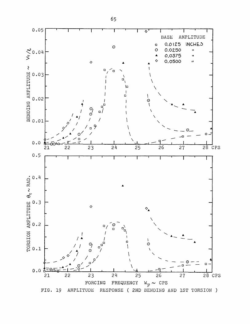
frequency of the third bending mode is about 19 cPS.The region between WF = 19 cPS to 22 CPS is relatively

quiet. Then another instaoility region is encountered wherethe beam oscillates predominantly in the second bending modeand twists in the first torsion mode. The amplitude responseis shown in Fig. 19.with the bending amplitude in an enlargedscale. As WF approaches 24 CPS, the second bending and firsttorsion amplitudes grow and at a certain frequency they arebigger for larger base amplitudes. The beam is stable and goesback to the same state when disturbed. The bending frequencyis about 7 CPS and goes down to 6 CPS at higher amplitudes. Asample record is shown in Fig. l6a. The amplitudes reach apeak near WF : 24 CPS. Here the bending frequency is about6 CPS and torsion frequency, about 18 CPS. The beam executesa large flapping motion. The amplitudes vary somewhatirregularly. A sample record at 0.0125 in. base amplitude isshown in Fig. l6b. The beam is released from the rest and theresponse is recorded at slow speed. The amplitudes of vibra-tion grow to a certain amplitude, then becomes more or lesssteady. The later portion is recorded at high speed to revealthe wave form. At higher base amplitudes the motion becomesmore irregular. Two sample response records at large attenua-tion are shown in Fig. l6c and l6d, for 0.025 in. and 0.0375in. base amplitude. The later record shows a beating phenomenanear WF = 23.3 CPS. These responses are basically nonlinearin nature. Behaviors become nonlinear for tip deflections

32

of 1 in. or more.As WF exceeds 25 CPS the beam quiets down for 0.0125 in.

base amplitude. For 0.025 and 0.0375 in. base amplitude themotion becomes relatively small as WF approaches 26 cps.Beyond this the beam still vibrates in second bending mode atabout 7 CPS and twists irregularly at high frequencies but theamplitudes are small. Beyond WF = 30 CPS the amplitudes risesharply indicating another instability region but this was notinvestigated here.

A concise summary of the typical response behavior ofthe beam is presented in Table 2 for each of the four baseamplitude motions tested.

33CHAPTER 4

CONCLUSIONS

The present report has investigated the dynamics oflateral bending and torsion vibration of a thin flexible beamunder vertical harmonic excitation, both theoretically andexperimentally. Only the linear equations are considered forthe theoretical analysis.

The governing equations for an initially straight beamfor small motion are two coupled homogeneous equations repre-senting lateral bending and torsion dynamic equilibrium.Since the experimental specimen had a static deflection due tobuilt-in imperfection, inclusion of this gives rise to forcingterms on the right hand side of the homogeneous equations.Using Galerkin's method with assumed normal modes one gets asmany equations as number of mode shapes assumed. These are tobe analyzed in time domain. The homogeneous part of theequations have the same characteristics as the Mathieu equa-

ltion. Because of the forcing terms on the right hand side,parametric and forced excitation coexist and the main inter-actions occur near the second instability region of Strutt'sdiagram. These coupled linear equations are complex enoughto forbid one from writing down the approximate closed formgeneral solutions as usually done for a one degree of freedomsystem, but the procedure for obtaining solutions has beenoutlined. The first and second instability regions for no

34

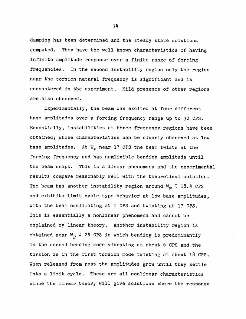
damping has been determined and the steady state solutionscomputed. They have the well known characteristics of havinginfinite amplitude response over a finite range of forcingfrequencies. In the second instability region only the regionnear the torsion natural frequency is significant ind isencountered in the experiment. Mild presence of other regionsare~also observed.

Experimentally, the beam was excited at four differentbase amplitudes over a forcing frequency range up to 30,CPS.Essentially, instabilities at three frequency regions have beenobtained; whose characteristics can be clearly observed at lowbase amplitudes. At WF near 11 CPS the beam twists at theforcing frequency and has negligible bending amplitude untilthe beam snaps. This is a linear phenomena and the experimentalresults compare reasonably well with the theoretical solution.The beam has another instability region around WF : 18.4 CPSand exhibits limit cycle type behavior at low base amplitudes,with the beam oscillating at 1 CPS and twisting at l1CPS.This is essentially a nonlinear phenomena and cannot beexplained by linear theory. Another instability region isobtained near WF : 24 CPS in which bending is predominantlyin the second bending mode vibrating at about 6 CPS and thetorsion is in the first torsion mode twisting at about 18 CPS.When released from rest the amplitudes grow until they settleinto a limit cycle. "These are all nonlinear characteristicssince the linear theory will give solutions where the response

35

WF 3 .frequency can only be ~ , 2 WF ••,WF, 2WF .••• etc., and cannotgive any limit cycle. Thus one has to go into the nonlinearformulation of this problem to predict such behaviors. Theresponse becomes nonlinear for tip deflection of 1 in. or more.The nonlinear terms are not quite well defined and one getsdifferent equations proceeding in different manners.

For future work one may look at the nonlinear problem andtry to explain the experimental results which are presented

1in detail. Bolotin has briefly discussed the nonlinearproblem but the solution is inadequate to explain the nonlinearbehaviors observed. Thus in working with similar structuralconfiguration and loading one has to carry out a carefulexperimental investigation without" relying entirely on thetheoretical linear analysis.

36

APPENDIX A

MODE SHAPES

The mode shapes in bending and torsion are chosen so asto satisfy the dynamic equilibrium in free vibration and theassociated boundary conditions4. They are

hk (~) Co5h AI<1. - C05Aktt - (Jk ( Sh'\h AK~ - Sin). k'1)

ex K (~) = .5 iY\. .ILk ~

where K refers to the mode shape.

AK and oK are tabulated in Ref. 4 part of which is reproducedbelow.

MODE oK AK A4K

1 0.73410: 1.8751 12.3622 1.01847 4.6941 485.523 0.99923 7.8548 3806.54 1.000043 10.9955 14617.0

37

APPENDIX BEVALUATION OF CONSTANT TERMS

1 2 1 2A, - J (hi) d1 - 1 Az = tChz) d1 = 1-

0

1 1 II 2P>I - J(h~')2d1 ='2.362 Bz. = Ie hz) d1 = 485.52

0 0

1 2. 1I i 2. II

C, - J (I-YI) 0< hi d1= 0.4206 Cz. = J(I-~)Qh2d1=-1.63610 0

1 2D - 5COC)d1 - 0.500 [ ex 1)ENOT~5 ()(1 1-

0

1 • 2H - 5(CX)d~= l.2 337

0

1 2 II

Cst = J (I-~) es hi d'1.o1 2 II

CS2. = 1 (I-~) Ss h2 dyto1 2 ..

S - f (1- ~) hS ex d~o

(B.l)

The constants CSl' CS2' and S are evaluated by assumingthat the built-in deflection and twist hB' SB and staticdeflection and twist hS' Ss are similar to the assumed first

38

bending and torsion mode shapes respectively and differ onlyin amplitudes.So we write

(B.2)

Vs _ h ( )t Bs 1 '1

and one needs to evaluate only TS and BS~ Since Eq. (B.2) mustsatisfy static equilibrium Eqs.(2.8), (2.9), we introduce themand apply Galerkin's technique using hl(n) and a (n) as theweighing functions respectively, to get

o (B. It)

39

using the definitions in Eq. (B.l). After slight manipulationand using the notations introduced in Eq. (2.15) they reduce'to

(B.5)

(B.6)

Solving for BS and TS

where

(B.7)

(B.8)

For our specimen there is no appreciable built in twist butVs is estimated to be 0.25 inches in negative Yo direction.Thus one need not measure BB and has

40

Bs - 0.25/21 = - 0.00521

SINCt:.

Ts - 0.002..37

Thus from Eq. (B.2a)

CS1 - - 0.00237 C,

C~2. - - O.OO237C2

5 - - o. 00521 C,

It may be noted from Eqs. (B.7), (B.8) that the static bucklingwill occur when FI = FIS with the natural free vibration modeassumption. For the experimental specimen F1 = 0.0735 andF1S = 0.4016.

41

REFERENCES

1. Bolotin, V.V., Dynamic Stability 'ofEla'stic Systems,Holden-Day Inc., San Francisco, California," 1964.

2. Chhatpar, C.K. and Dugundji, J., Dynamic Stability ofPendulum Under Parametric Excitation, M.I.T. Aeroe1asticand Structures Research Laboratory, Report TR 134-4,AFOSR-69-0019TR, December 1968.

3. Chhatpar, C.K. and Dugundji, J., Dynamic Stability ofPendulum Under Coexistence of Parametric and ForcedExcitation, M.I.T. ASRL Report TR 134-5, AFOSR-68-0001,December 1967.

4. Young, D., Vibration of Rectangular Plates by Ritz Method,Journal of Applied Mechanics, 17, 4, pp. 448-453, 1950.

42

TABLE 1

BEAM PARAMETERS

Length 1, = 24.0 in.Width d = 3.0 in.Thickness b = 0.02 in.Material = AL 606l-T6Density p = 0.000253 lb-sec2/in~Modulus of Elasticity E = 107 psiPoisson's Ratio 'V = 0.3First bending mode natural frequencyW1h = 1.08 CPS (Theory 1.115 CPS)Second bending mode natural frequencyW2h = 7.00 CPS (Theory 6.988 CPS)First torsion mode natural frequencyWa = 17.0 CPS (Theory 17.12 CPS)

8 -4 2 2m = pbd = 0.151 x 10 1b-sec /in

lm = ~2 (b2+d2) -4 2= 0.1139xlO lb-sec

I L db3 2.0x10-6 in4= =12J L db3 8 -6 in4= = .0xlO3

43

TABLE 2

TYPICAL RESPONSE

BASE AMPLITUDE 0.0125 IN.W t

F

16.217.1*17.218.4*

19.023.4*

24.0

24.6*

2.50

BENDING MOTIONff

NegligibleSmall, w=17.lNegligibleModerate Steady in IBM.W=l.OGiven small kick-decaysGiven big kick-aboveresponseSmall W=19.0Moderate, Steady in 2BM.W=6.3Large, Steady in 2BM.w=6.0Large, Steady in 2BM.w=6.3Released from rest-grows to above.Negligible

TORSION f-10TION+

Small, Steady W=16.2Moderate, Steady W=11.lSmall, Steady W=11.2Large, Steady W=11.3

NegligibleModerate, SteadyW=11.0Large, Little unsteadyw=18.0Large, Little unsteadyW=18.0

Small, Steady W=25.0

tAll Wand WF are in cycles per second.tt IBM = 1st Bending Mode; 28M = 2nd Bending Mode+ Always in 1st Torsion Mode.* Records shown in figures.

44

TABLE 2 (CONTINUED)


F

15.017.017.418.5*

20.023.0

24.0*

25.5

27.2

BENDING MOTIONtt

NegligibleNegligibleNegligibleModerate, Steady in IBMW=0.9 with 18 CPSsuperimposed.Given small kick-decaysGiven big kick-aboveresponse.Small, Steady W=20.0Moderate, Steady in2BM. W=6.2Large, Irregular in2BM. W=1.0Large Irregular in2BM. W=1.0Moderate, in 3BM, W=19.0Given small kick-in2BM. W:7.0

TORSION MOTION+

Small, Steady W=15.0Moderate, Steady W=17.2Small, Steady W=17.4Large, Unsteady,Varying amplitude.W:17.5

Small, Steady W=20.0Moderate, Steady.W=17.0Large, Irregular.W=18.0Large, Irregular.W=18.0Moderate, IrregularMany harmonics present.

45

TABLE 2 (CONTINUED)

Moderate, SteadyW=16.8

NegligibleTORSION MOTION+BENDING MOTIONtt

Small, Steady in 2BMW=7.0Small, Steady in IBMW=16.8

BASE AMPLITUDE 0.0375 IN.W tF

7.0

16.8

17.018.0

18.419.3*

Snap by itselfModerate, Steady in IBMW=0.9 with 18 CPSsuperimposedLightly kicked, snapSnap by itselfLarge, Irregular in IBMInitially-none. Lightlykicked-above response

Snap by itselfLarge, Unsteady,Varying amplitudeW=17.0

Snap by itselfLarge, IrregularW:17.0

21.023.3*

Small in 3BM. W=19.0Large, Beating type in2BM. w:6.0

Small, W=21 and 86Large, Beating typew:18.0

24.4 Large, Irregular in 2BMw:6.0

Large, IrregularW:17.0

27.0 Moderate, Irregular in2BM. W:7.0

Large, Irregular,Many harmonics present

46

TABLE 2 (CONCLUDED)


F

7.016.4

17.017.5

18.7*

21.0

23.0

25.4

29.0

BENDING MOTIONtt

Small, Steady in 2BMW=7Negligible. Sway toone side.Given kick-snapSnap by itselfInitially none.Given small kick-snapReleased from rest-Amplitude grows slowlyto snapSmall, Steady in 3BMW=19.Kicked-snap, eventuallycomes back to aboveLarge, Irregular in 2BMw:6.0Large, Irregular flappingin 2BM. w:6.0Released from rest-grows to aboveSmall, Irregular in2Br~. W:7. 5

TORSION MOTION+

NegligibleLargel Steadyw=16.Q

Snap by itselfLarge, UnsteadyW::17.0Torsion frequency17.0 before snapping

Moderate UnsteadyW=2l and 86

Large IrregularW:17.0Large, Irregular

Large, Irregular

48

CLAMPED

STRAIN GAGES

STRAIN GAGES

,-

/TcCORDER ,Be;

TTI

~ J

TORE

BASE tMOTION

FIG. 3 SCHEMATIC DIAGRAM

FIG. 4 COORDINATE

18

49

16

14

12

1ST TORSION

~3 10"'J

""-u..3

( 8

~0z 2ND BENDINGw:::> 6GJW0::I:":Y

0z 4H00::0I:":Y MAXIMUM OPERATING POINT

21ST BENDING

o0.0 0.002 0.004 0.006 0.008 0.01 0.012

BASE AMPLITUDE rv DIe>

FIG. Sa FIRST INSTABILITY REGION

50

9

8 1ST TORSION..c3(\J

""- 711.

3

6?

>t0 5z~~a~0::~ 4eJz 2ND BENDINGH00::0~ 3

2

MAXIMUM OPERATING POINT

1ST BENDING

0.0120.010.0080.0060.002 0.0040.0o

1

BASE ArJIPLITUDEI"'>J U 1 BFIG. 5b SECOND INSTABILITY REGION

51CI)

CI)

P...P...

00

~~co

coH

MM

Lf'\C

I)

0P...

I()

0?

t-t-

~i1M

M~

Q:=;

::J

----rE-tH

(j

CI)

f-=!Z

~H

\.0\.0

:>.,.....

P-.r-i

M,2:.,~

;EC

I):..r.:t

<x:Z

Q0

Q~

H::J

CI)

(j

E-ic::x:

0W

Hc:o

Z0.::

Lf'\If\

f-=!M

MP...i.8

r.i1~

f-=!m

r.ilc::x:E-t

E-iC

I)c::x:

zco

coE-l

:::>C

I)

~

jQ~

t-;I~

t-E-iC

I)

f-=!c::::0

\.0HE-ir.il0.::0r.il::r::E-tt>Lf'\

M

c.~Hr:Y

0a

aLf'\

Ma

a(Y

)(\J

M0

aa

aa

a0

0

Ij;LA

•dW'f

DNIGNtIH•G'fH

.le~

•dIrI'fNOISHO;L

52

18

16 TORSION

.s:.......3 III"1

""II312

(

:>iu 10Z~1::J(SfLl0::~y

8C);-:?:HU~0P:. 6

II

2

~ MAXIMUM OPERATING POINT

IS'll BENDING

00.0 0.002 0.004 0.006 0.008 0.01 0.012

BASE AI.IPLITUDE rv U1B

FIG. 6a FIRS'll INSTABILITY REGION( TWO MODE APPROXIMATION )

9

8

..cT"1 73

~"'-

U-

S 6

(

>t0 5zw:::>aw~I:i:-f 4~...."........H0~0

3I:i:-f

2

1

53

1ST TORSION

/" MAXIMUM OPERATING POINT

1ST BENDING

00.0 0.002 0.004 0.006 0.008 0.01 0.012

BASE AMPLITUDE f'...J U15

FIG. 6b SECOND INSTABILITY REGION

( THO 110DE APPROXIIvlATION)

54BOxi---,.----r--r--~-_r_-_.__- _ ___,-__r-_,...-__r_-_r_-.,._____,

6

rild 4~d

OxZ Ox0 ~HCI) 2 ~0::08

00 2 4 6 8 10 12 BOX

BENDING GAGEFIG. 7 HEADING IN TORSION GAGE FOR PURE STATIC BENDING

BOXr-__,.----r--r--~-_r_-....._- _ ____,r____,.-~-___,_-__._-_r____5

4

3

2

1

0.0

DYNAMIC

0.01

xSTATIC

1ST TORSION MODE

0.02 e, 'V RAD.

FIG. 8 TORSION GAGE CALIBRATION CHART

55

4

3

2

1

o0.0 0.05

• DYNAMICX STATIC

0.10

BOX8

0.10

3. 3RD BENDING MODE2. 2ND BENDING MODE1. 1ST BENDING MODE

0.05

DYNAMIC

4

2

OF---""'_--I-_....L.-_...£----.l~_"_ _ __&... _ __L___""____..I _ __I__~ _ _L____I

0.0

6

FIG. 9 BENDING GAGE CALIBRATION CHART

56

0.100.050.00.0

~t. s~o • 05 r----r---r----r--.,.------,----,...---r--~-r__~-__r_-__r_-~____,

0.01

0.02 1----'

0.04

FIG. 10 DAMPING RATIO IN 1ST AND 2ND BENDING MODE

0.01

0.03

0.02

0.00.0 0.10 0.20

FIG. 11 DAMPING RATIO IN 1ST TORSION MODE

1ST B[NDING

15T TOI2SIO

1 ~E.C

• • • • • • • • • • • • • • • • • • • • • • • • • • • • •

FIG. 12 SAMPLE FIRST BENDING DECAY RECORD

B~ND1NG

_ 100

\.

- !J.

-0

- 10.

1ST TORS 1ON

1 -SE.e

FIG. 13 SAMPLE FIRS T TO 510 DECAY RECORD

J ST BE.NDING

1ST T0l2S10Npl-

CA', • \7-1 CPSUs • 0'0\2:)' .

(&A~E. AWPUTUD£,)

t---- 1Sf-C --~

FIG. 14 STEADY STATE RESPONSE AT U1F= 17.1 CPS

3'/ IN.- 2."

-2"

-~"

"- 10

6JF = \S.4 CP5Uti ~ 0-0125 IN.

(BAS~ "Mf>~\TUD~)

J~T BE.NDlN

1ST T 5?510

FIG. 15a. RESPONSE WITH SMALL AND LARGE KICK AT WF= 18.4 CPS

~-, ...2.--

•3_

16T BE.NOIN

~

~\Ie • 0'0125, 0 !-

(f>A)E AMPLITUDE) •I,...

'IL

1ST TOI2SIOt-J

..-..-----. 1 SEe..

• • I •

FIG.15b

- 2// IN.

#-2

LIMIT CyCLE RESPONSE AT '-"F = 18.4 CPS

15T BENDING

()JF • 18.~ CPSUI> .. 0.025 IN,

(f>ASE AMPLITUDE)

FIG, 15c L I MIT CYCLE

1ST TO 510N

RESPO SE AT '-"F= 18.5 CPS

"- to IN.

-5"

<J'rr == '~.3cPSUe. - O'037~ aN.

(6A5E AMPLaTUOE). \ \ ~

BENDI G

TOR~lON

FIG. 15d RESPONSE WITH LIGHT KICK AT ~F = 19.3 CPS

- 3" I"'.

- 2" BENDI G

A f. V I, I ; , l

"i •1 I '

I. ,_ 3"

:., I

~-----1 & C .....;I~-...-i

(rjF:a 18?CPS TOlCSIONUti 20'050 rH.

(f>ASE AMPLITUDE)- lot

- ~.- '5"

____ ....:;,::._--;r.,,\l ../II,l:~:.'i~-------...;'oJ.;'l:

FIG. 15e S APPI G WHEN RELEASED FRO REST AT lJJF=18.7 CPS

,o~~F. 23--4 cPsU,. o'o,tD 'N. 0-

(~A.sE A PLlTUDE)!/

lO-

2 D BE.t-lDING

1ST TO£SION

FIG. 160. STEADY STATE RESPONSE AT U'F= 23.4 CPS

2ND 8E.NDIN

-I"

1~T TO 510

.-15 1 &EC EC---...-t

FIG. 1Gb LIMIT CYCLE RESPONSE AT (t}F= 24.6 CPS

OJ, ,..2<4.0 CPSu. '"0"025 I .

(f>AS£ A"'PLI TU.DE.)

2ND BEN I

Flf~T TO~ 10

t---- 1 SEe .,

FIG. 16c RESPONSE AT U)F = 24.0 C PS

.-0

WF = 2~'~ CPSUt> "" O'O~75 IN.

(r>ASE. AMPLITUDE.)

FIG. 16d BEATING RESPONSE AT WF= 23.3 CPS

63

aao

No

rJ1P..(.)

a(Y')

()0

rI

0

..I

'r:Y

0~

,I

I..I

0\

:>i...,

00

\Z

~~

II

:::>a./

./W

---_

0-

J:t:()

r:Ym

00-

-0-

- -N

CJI

Z(!)

0H

0'

-0

..-0

cr::-0

0()

0-

E>-......

r=.t-

...---..... ,

...--00

......-

...,\

()....,

(/)0\

'or>

\

00.10

fiJ,/

U)

z0N

P..C

I)

..Lr.1J:t:

<:)<:>

f=-l..

Q4

:::>~...

0::-Ptf'=;"O

Hl-l_

4_..

0......

A-I'..

'0'

,,---0

-0..........

,0~

-'0

4'\

<:t:......

..0,

\\t-

o"r-l

'.L

f\,...;

0J-~r~!~

..

o

NL

..-_..L

._

_L

-_

--L

__

.L-_

--L_

_...L

.-_.....;;Jr-i

aa

mao

,...I..'..,/

//

/()

_..

_0

..---

...a

WQV

)

::>LL1

8:r

H0

::::-

::H

ZP..~c:x:

([)OlO

0\.Of'-..

0~

NN

t<110C

I)0

00

0c:x:

00

'00

c:Q

00

~()

NL

..-...........L.--L_"---1--l---L_.L-....I..-~---&_.L--'----'rl

r--,-~_

-..--_

_-...-....-_

_-....C

I)

P..oa(Y

)I/)0-U2

64

BASE AMPLlrrUDEo 0.0\25 INCHE.So 0.02.50 II

A 0.0375 II

o 0.0500 u

0.0

II\<\- ~21 CPS

III\\t- rrtt> - :J

20

II

I

, /0-011(0. ,'00 \ I

'19 I IJ I ' _. I \

).' J, \• ..~~C0'1i;) I/O I '0.....cp 0

14 15 16 17 18 19

~ 0.15"":>

~~Q

~ 0.10HHP-.~~CJ:z:~ 0.05:z:~t:o

CPS

1ST TORSION )

~ JoQ::>

I8 ..HH ,0 I ....0\P-. 0.10 00

~ I 0 I~ • I I:z: I I 0, I0 I I IH 0/ /CI) 0 Ip:::: • /01 I0 / / / dl, \8 0.05 I0 / / / ~I

\ I/~ / I \ \.. o / \/0 ...- • / \ I \- ..- ........0/0 \ \ 0 \ \

oDe:( / 00.0 ~15 17 18 19

FORCING FREQUENCY WF IV CPSFIG. 18 AMPLITUDE RESPONSE ( 1ST BENDING AND

0.20.

Q~p::::~.-0 .15

<D

65

0.05BASE AMPLITUDE

o 0.0 \Z 5 \NCHE.~o 0.02.50 II

A 0.0375 ..o 0.0500 II

0-

---CI -

27

-- - _0_

\

\\\

"\o\\

\'\.

25

\o

\

\0I

o

o

2322210.0

~

2i 0.03:::>8H~P-.~<x: 0.02CJ:z;HQ:z;~~ 0.01

~ 0.04:>

0.5

0--- -0--_0-

\o\

"\

\\

\

EJ

I/ A

/ I

-o . 0 D-~.a..a--L..-;;;.-....L_--L_--L._--L._--L-_.:...LII-_-J.::::=----L-_..l-_..l-_.L..-_a........J

21 22 23 24 25 26 27 28 CPSFORCING FREQUENCY WF~ CPS

FIG. 19 AMPLITUDE RESPONSE ( 2ND BENDING AND 1ST TORSION )

o 0.4<x:P::

<~~ 0.3Q:::>8H~P-.~ 0.2:z;oH(/)P::~ 0.1

66

0.15~

...........

~~

ri1~~ 0.10Hl-lP1:~~~

o. 0 ~&.-.014 15

00o00o

0.20.

Q~P:::

2...0.15

<D

~Q~8H..-l~ 0.10~:z:oHU)~o8 0.05

o

THEORYEXPERIMENT

0 0.012.5 IN.0 0.0250 n

0 • 0.0375 II

• 0 0.0500 It

0BASE AMP.

o00

o

14 15

FIG. 20

16FORCINGTHEORY

17 18 19 20FREQUENCY WFIVCPS

AND EXPERIMENT COMPARISON

CPS

core.ac.uk · the dynamics of lateral bending and torsion vibration of a ... excitation and...

Documents