cook - experiment on the linear increase in efficiency ... · experiment on the linear increase in...

Cook: Experiment on the Linear Increase in Efficiency Vol. 9 82

Experiment on the Linear Increase in Efficiency with Multiple Moving Magnets over Pulsed Inductors

Jeffrey N. Cook 1727 Christopher Lane, Maumee, OH 43537

e-mail: [email protected]

I have prepared an experimental apparatus consisting of an inductor and five reversible DC motors, used as DC electrical generators, hooked to ring magnets suspended above the inductor whose radii are ninety de-grees from the radius of the inductor and hooked from belts to the motors. I then DC pulse the inductor caus-ing the magnets to experience three motions, but confine all energy with the belt to the rotational motion alone, which turns the motors. I include many iterations of varied waveforms and different numbers of generators in order to measure the power IN to the inductor and OUT from the reversible DC motors, used as electrical gen-erators (not hooked to the same electrical circuit with the inductor in any way). I have measured over many it-erations and varied resistive loads (though only a 10 load is described in this paper for sake of straight for-ward simplicity) that the COP (the coefficient of power OUT divided by power IN) is greater than unity of sig-nificant magnitude when the amplified signal frequency input to the inductor is above a certain threshold, while the power IN is reduced below another threshold.

1. Introduction

This experimenter has found through past experiments and observations [12] that a permanent magnet placed in the proximi-ty of a DC-pulsed inductor experiences four motions: 1) preces-sion, 2) nutation, 3) rotation and 4) orbit. It has been hypothesized [12] that the precession is electro-magnetic (E & B Fields) in na-ture, as it is synchronous with the input signal frequency. The nutation may be due to the A Field (also called the “Vector Mag-netic Field”), as there are some iterations that suggest that de-pending on the signal’s frequency, duty cycle and dimensions of the inductor, the nutation can be made to be synchronous with the signal frequency when the precession frequency drops off to zero. However, the frequency of the rotation and orbit tend to be independent from the frequency in all cases yet explored. The orbit frequency also tends to be of a lower magnitude and con-stant, but by turning a ring magnet ninety degrees from the in-ductor’s face, the rotation frequency tends to increase exponen-tially as it nears the center of the coil. This experiment explores the rotational motion’s energy and eliminates the nutation com-pletely by placing the ring magnet on a brass rod. Thus, three motions remain, but only one is measured.

Fig. 1. Top View Drawing of the Magnet-Inductor Setup with Three Motions on a Ring Magnet Suspended on a Brass Ring

The rotational direction (which may be in the opposite direc-tion, depending on the setup) of the ring magnet (whose radius is ninety degrees to the inductor’s radius) is represented above with the blue arrow, the precessional directions (always back and forth) with the red arrow and the orbital direction (which also may be in the reversed direction depending on the setup) with the violet arrow. The nutation is eliminated with this setup by being suspended on the brass ring, which restricts its motion to or away from the center (nutation). The yellow-orange area above represents the magnet wrapping wire part of the inductor, the gray area represents the ferrous material inside the windings and the white area at the center represents and air hole.

When the inductor is DC-pulsed the motions above are repet-itive and continuous so long as the power input is significant enough to affect the mass of the magnet. When the ring magnet is suspended on a brass rod instead of a brass ring, the motions are all the same except for the orbit, which then oscillates back and forth to the rod’s ends (provided there is force (or object) at the ends, restricting the magnet from traveling off the face of the inductor—provided the rod is restricted from vibrating signifi-cantly, in which case the orbit cancels altogether).

Fig. 2. Top View Drawing of the Magnet-Inductor Setup with Three Motions on a Ring Magnet Suspended on a Brass Rod

Albuquerque, NM 2012 PROCEEDINGS of the NPA 83

In either Fig. 1 or Fig. 2, the precession and rotation are unaf-fected by anything that affects the orbit. Additionally, since the nutation is eliminated without affecting the precession or rota-tion or orbit in any way, the result of the prior experiments [12] support the hypotheses that these are all independent motions. Independent motions having independent frequencies, inde-pendent velocities and independent forces lead the author to conclude from the past experiments that these independent mo-tions arise from independent fields of force, but concluded cau-tiously.

While the fields of force generating the precessional motion are well defined with Tesla’s “Egg of Columbus” [3], first shown publicly by Nikola Tesla and George Westinghouse in 1893 at the Chicago Columbian Exposition in order to demonstrate the be-haviors of AC current, as an oscillation of the E Field and the B Field, his demonstration with AC pulsed inductors restricts the motion to the dead-center of the coil arrangements (minimum number of coils required is three). My studies are with a single DC-pulsed inductor where the motions are generated anywhere else but dead-center. Additionally, as there are more than just two motions (back and forth, precession) with this setup, the question has arisen to the author as to what the additional fields causing the motions could be, as there are typically thought to exist only four fields of force acting between two permanent magnets [9]: B, A, E and N (gravity), while the gravitic field be-tween two magnets does not approach the magnitude of forces at play in the above setup [6]. While it is yet possible to consider that these four fields alone could be responsible for the four mo-tions if the precessional motion of the magnet were alone respon-sible by a directional-changing B or E (exclusively) Field, the resulting additional force would require the gravitational field to be at play. This experimenter does not consider this however, as previous experiments [12] suggest yet another field may be pre-sent at the poles of the magnets that is not sufficiently described or defined by their magnitude measurements, typically symbol-ized by the H vector field or polarization force p [16], as fields of force as defined by Gauge Theory [7].

While such hypothetical discussions would take numerous more experiments to rule in or out such thoughts, this experi-ment relies only on one, one that could easily rule in or out the notion of the additional field this experimenter believes is at play in this setup (the Z Field, or Zero Point Energy Field), as if the ground state of the energy of the system were increased, then it would be supportive of the notion of additional fields present in a DC-pulsed inductor (as opposed to non-pulsed DC). The zero point energy of any mechanical system is defined as the sum of all the energies of all the fields in the system [13]. Thus, increase the number of fields and the energy ground state increases. Without adding extra power to the inductor, extra power (and energy, AKA work) could hypothetically be extracted by simply adding additional magnets to the inductor’s proximity.

2. Hypothesis

I think that the power efficiency of a mechanical system hav-ing multiple moving magnets over a DC-pulsed inductor would increase linearly with each additional identical magnet applied because the angular momentum of all the magnets remains the

same under equivalent circumstances and increases in angular momentum with an increase in frequency.

This experiment would not expect the Laws of Thermodynamics to be broken; rather that they only apply to closed systems. This does not require a system to be prevented from greater entropy at some point in time between 0t and t , just that it can experience fluctuations in its amount of entropy gain within that infinite amount of time, thereby allowing it to have lesser entro-py for some 0t (ie. the motion of a system cannot be perpetu-al, but its kinetic energy can exist any length of time less than infinity, even millions or billions of years) [15]. Thus, if the above hypothesis is supported with this experiment, then the resulting physical requirement is that a DC-pulsed inductor cre-ates an open system (symmetry is broken), which would not ex-perience the same limitations as an AC-pulsed inductor or a non-pulsed DC inductor [9]. An open system would then not be lim-ited to the power input to the coil; rather, free to interact with other fields, thereby drawing on energy elsewhere in order to satisfy the Principle of Least Action [4], as will be described later in the analysis and conclusion.

In accordance with Gauge Theory, each of these repetitive four motions mentioned above are independent if they have inde-pendent frequencies, defining them as independent actions [7]. Due to the Noether Theorem, with each independent action, an independent gauge field, and independent gauge flow and inde-pendent gauge boson is present [7]. While the additional gauge boson for each of these motions could be argued to be the addi-tion of another photon (the gauge boson for the electromagnetic field), the energy of the ground state still should increase. How-ever, if the energy of the magnet-DC-pulsed inductor system were to increase linearly (or greater than linearly) with each ad-ditional magnet, then the law of Conservation of Energy could not be valid if photons were the only additional gauge bosons, as Planck’s Constant h would not retain the same numerical value based on the energies and frequencies of the system [15]. How-ever, it is not this experimenter’s suggestion that the law is un-sound, as numerous experiments and theorems over the centu-ries have supported it. Thus, the hypothesis above (if supported with this experiment) would cause support also for the hypothe-sis that such a system could not be symmetric and therefore could not be explained using the algebraic Lie Groups [1]; rather, it would require the addition of Topological Groups, groups that best describe zero point energy [2,14], whereby the law would not apply as it would not be a system functioning on quantum mechanical factors.

3. Experimental Design

The method for testing the efficiency of the above mentioned system was DC electrically generated power from the rotational motion of the magnets only. Measurements of (rotational) angu-lar velocity could have also been constructed (and was consid-ered), but since electrical power is sent to the coil, it seemed most fitting to measure electrical power out. An inductor and appa-ratus was constructed from components that are readily available in most cities.


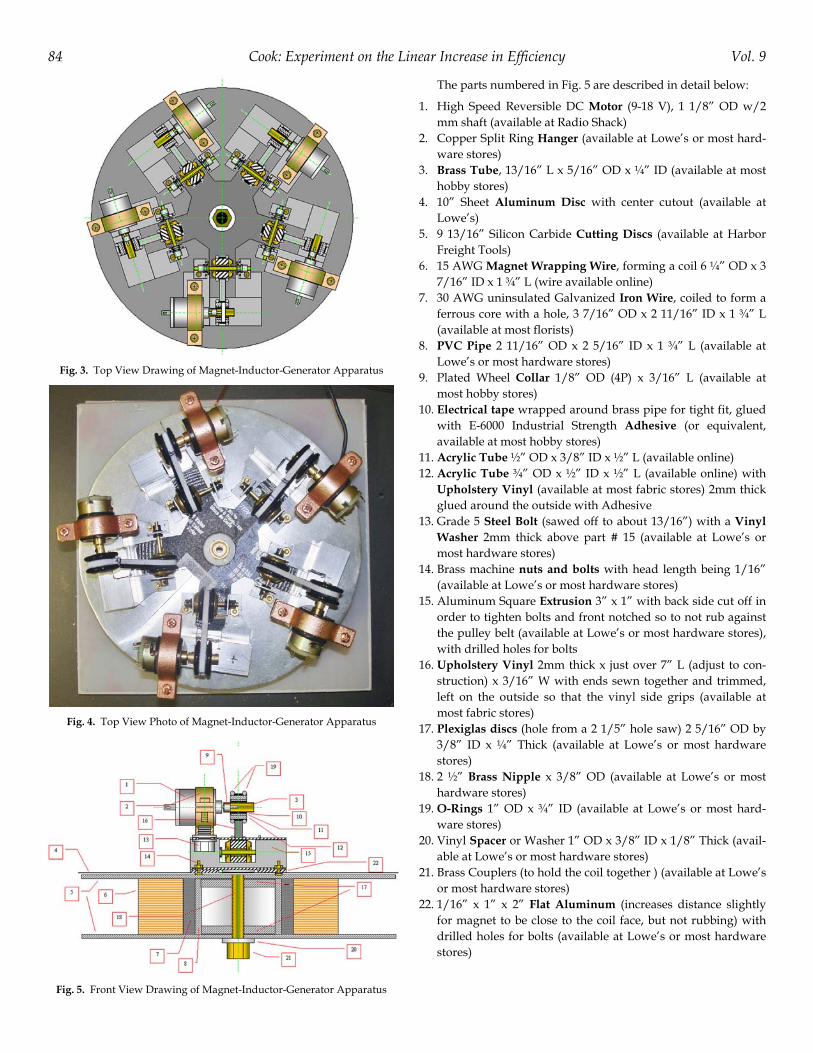
Fig. 3. Top View Drawing of Magnet-Inductor-Generator Apparatus

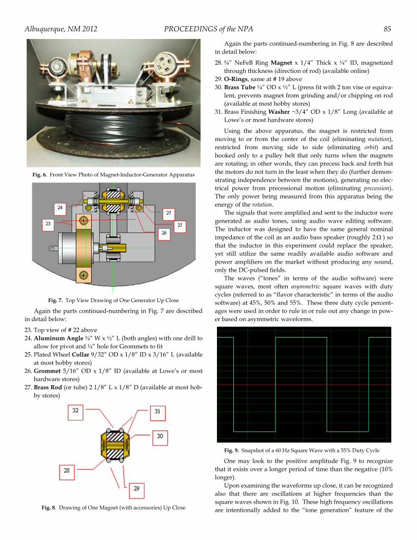
Fig. 4. Top View Photo of Magnet-Inductor-Generator Apparatus

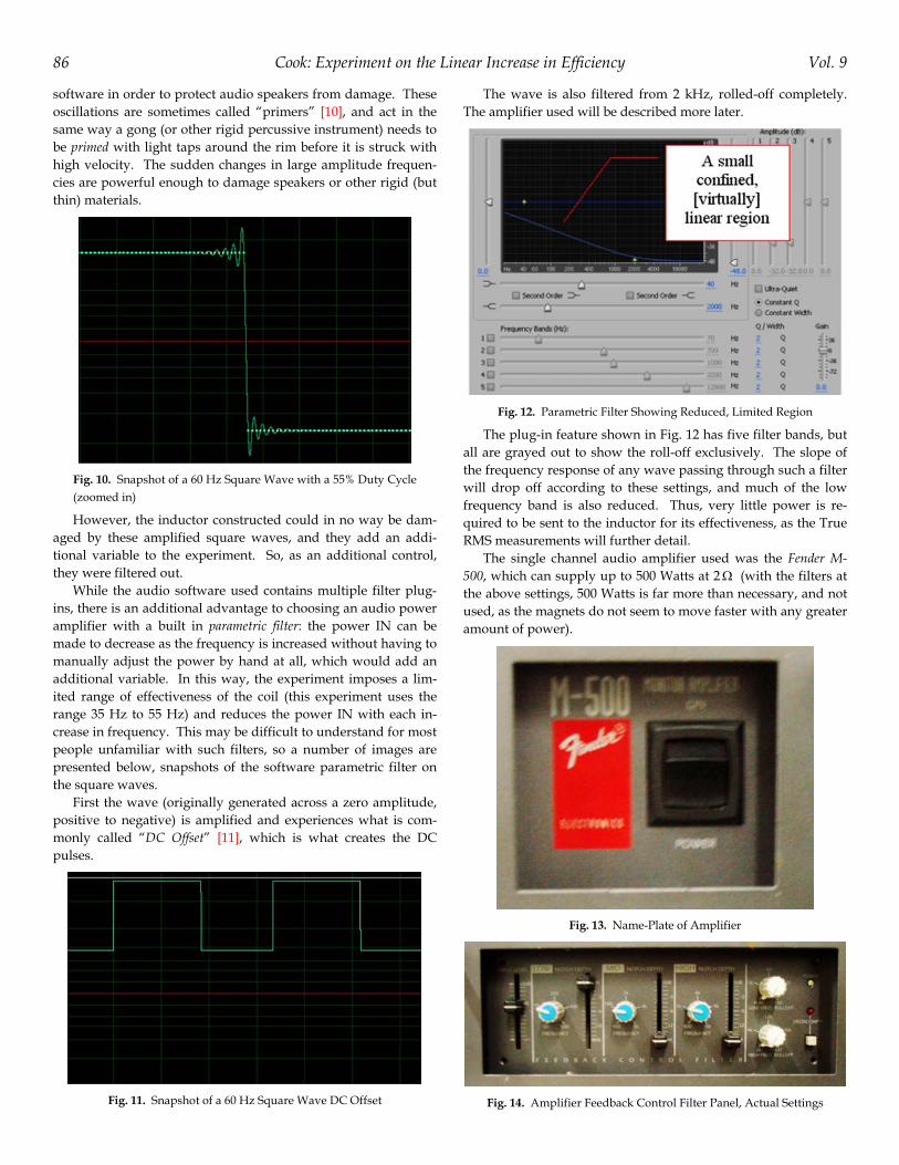
Fig. 5. Front View Drawing of Magnet-Inductor-Generator Apparatus

The parts numbered in Fig. 5 are described in detail below:

1. High Speed Reversible DC Motor (9-18 V), 1 1/8” OD w/2 mm shaft (available at Radio Shack)

2. Copper Split Ring Hanger (available at Lowe’s or most hard-ware stores)

3. Brass Tube, 13/16” L x 5/16” OD x ¼” ID (available at most hobby stores)

4. 10” Sheet Aluminum Disc with center cutout (available at Lowe’s)

5. 9 13/16” Silicon Carbide Cutting Discs (available at Harbor Freight Tools)

6. 15 AWG Magnet Wrapping Wire, forming a coil 6 ¼” OD x 3 7/16” ID x 1 ¾” L (wire available online)

7. 30 AWG uninsulated Galvanized Iron Wire, coiled to form a ferrous core with a hole, 3 7/16” OD x 2 11/16” ID x 1 ¾” L (available at most florists)

8. PVC Pipe 2 11/16” OD x 2 5/16” ID x 1 ¾” L (available at Lowe’s or most hardware stores)

9. Plated Wheel Collar 1/8” OD (4P) x 3/16” L (available at most hobby stores)

10. Electrical tape wrapped around brass pipe for tight fit, glued with E-6000 Industrial Strength Adhesive (or equivalent, available at most hobby stores)

11. Acrylic Tube ½” OD x 3/8” ID x ½” L (available online) 12. Acrylic Tube ¾” OD x ½” ID x ½” L (available online) with

Upholstery Vinyl (available at most fabric stores) 2mm thick glued around the outside with Adhesive

13. Grade 5 Steel Bolt (sawed off to about 13/16”) with a Vinyl Washer 2mm thick above part # 15 (available at Lowe’s or most hardware stores)

14. Brass machine nuts and bolts with head length being 1/16” (available at Lowe’s or most hardware stores)

15. Aluminum Square Extrusion 3” x 1” with back side cut off in order to tighten bolts and front notched so to not rub against the pulley belt (available at Lowe’s or most hardware stores), with drilled holes for bolts

16. Upholstery Vinyl 2mm thick x just over 7” L (adjust to con-struction) x 3/16” W with ends sewn together and trimmed, left on the outside so that the vinyl side grips (available at most fabric stores)

17. Plexiglas discs (hole from a 2 1/5” hole saw) 2 5/16” OD by 3/8” ID x ¼” Thick (available at Lowe’s or most hardware stores)

18. 2 ½” Brass Nipple x 3/8” OD (available at Lowe’s or most hardware stores)

19. O-Rings 1” OD x ¾” ID (available at Lowe’s or most hard-ware stores)

20. Vinyl Spacer or Washer 1” OD x 3/8” ID x 1/8” Thick (avail-able at Lowe’s or most hardware stores)

21. Brass Couplers (to hold the coil together ) (available at Lowe’s or most hardware stores)

22. 1/16” x 1” x 2” Flat Aluminum (increases distance slightly for magnet to be close to the coil face, but not rubbing) with drilled holes for bolts (available at Lowe’s or most hardware stores)


Fig. 6. Front View Photo of Magnet-Inductor-Generator Apparatus

Fig. 7. Top View Drawing of One Generator Up Close

Again the parts continued-numbering in Fig. 7 are described in detail below:

23. Top view of # 22 above 24. Aluminum Angle ¾” W x ½” L (both angles) with one drill to

allow for pivot and ¼” hole for Grommets to fit 25. Plated Wheel Collar 9/32” OD x 1/8” ID x 3/16” L (available

at most hobby stores) 26. Grommet 5/16” OD x 1/8” ID (available at Lowe’s or most

hardware stores) 27. Brass Rod (or tube) 2 1/8” L x 1/8” D (available at most hob-

by stores)

Fig. 8. Drawing of One Magnet (with accessories) Up Close

Again the parts continued-numbering in Fig. 8 are described in detail below:

28. ¾” NeFeB Ring Magnet x 1/4” Thick x ¼” ID, magnetized through thickness (direction of rod) (available online)

29. O-Rings, same at # 19 above 30. Brass Tube ¼” OD x ½” L (press fit with 2 ton vise or equiva-

lent, prevents magnet from grinding and/or chipping on rod (available at most hobby stores)

31. Brass Finishing Washer ~3/4” OD x 1/8” Long (available at Lowe’s or most hardware stores)

Using the above apparatus, the magnet is restricted from moving to or from the center of the coil (eliminating nutation), restricted from moving side to side (eliminating orbit) and hooked only to a pulley belt that only turns when the magnets are rotating; in other words, they can precess back and forth but the motors do not turn in the least when they do (further demon-strating independence between the motions), generating no elec-trical power from precessional motion (eliminating precession). The only power being measured from this apparatus being the energy of the rotation.

The signals that were amplified and sent to the inductor were generated as audio tones, using audio wave editing software. The inductor was designed to have the same general nominal impedance of the coil as an audio bass speaker (roughly 2 ) so that the inductor in this experiment could replace the speaker, yet still utilize the same readily available audio software and power amplifiers on the market without producing any sound, only the DC-pulsed fields.

The waves (“tones” in terms of the audio software) were square waves, most often asymmetric square waves with duty cycles (referred to as “flavor characteristic” in terms of the audio software) at 45%, 50% and 55%. These three duty cycle percent-ages were used in order to rule in or rule out any change in pow-er based on asymmetric waveforms.

Fig. 9. Snapshot of a 60 Hz Square Wave with a 55% Duty Cycle

One may look to the positive amplitude Fig. 9 to recognize that it exists over a longer period of time than the negative (10% longer).

Upon examining the waveforms up close, it can be recognized also that there are oscillations at higher frequencies than the square waves shown in Fig. 10. These high frequency oscillations are intentionally added to the “tone generation” feature of the


software in order to protect audio speakers from damage. These oscillations are sometimes called “primers” [10], and act in the same way a gong (or other rigid percussive instrument) needs to be primed with light taps around the rim before it is struck with high velocity. The sudden changes in large amplitude frequen-cies are powerful enough to damage speakers or other rigid (but thin) materials.

Fig. 10. Snapshot of a 60 Hz Square Wave with a 55% Duty Cycle (zoomed in)

However, the inductor constructed could in no way be dam-aged by these amplified square waves, and they add an addi-tional variable to the experiment. So, as an additional control, they were filtered out.

While the audio software used contains multiple filter plug-ins, there is an additional advantage to choosing an audio power amplifier with a built in parametric filter: the power IN can be made to decrease as the frequency is increased without having to manually adjust the power by hand at all, which would add an additional variable. In this way, the experiment imposes a lim-ited range of effectiveness of the coil (this experiment uses the range 35 Hz to 55 Hz) and reduces the power IN with each in-crease in frequency. This may be difficult to understand for most people unfamiliar with such filters, so a number of images are presented below, snapshots of the software parametric filter on the square waves.

First the wave (originally generated across a zero amplitude, positive to negative) is amplified and experiences what is com-monly called “DC Offset” [11], which is what creates the DC pulses.

Fig. 11. Snapshot of a 60 Hz Square Wave DC Offset

The wave is also filtered from 2 kHz, rolled-off completely. The amplifier used will be described more later.

Fig. 12. Parametric Filter Showing Reduced, Limited Region

The plug-in feature shown in Fig. 12 has five filter bands, but all are grayed out to show the roll-off exclusively. The slope of the frequency response of any wave passing through such a filter will drop off according to these settings, and much of the low frequency band is also reduced. Thus, very little power is re-quired to be sent to the inductor for its effectiveness, as the True RMS measurements will further detail.

The single channel audio amplifier used was the Fender M-500, which can supply up to 500 Watts at 2 (with the filters at the above settings, 500 Watts is far more than necessary, and not used, as the magnets do not seem to move faster with any greater amount of power).

Fig. 13. Name-Plate of Amplifier

Fig. 14. Amplifier Feedback Control Filter Panel, Actual Settings


Input Level 0 dB Low Band Notch 70 Hz Low Notch Depth 0 dB Mid Band Notch 700 Hz Mid Notch Depth Max High Band Notch 7 kHz High Notch Depth Max Low Frequency Rolloff Flat High Frequency Rolloff 2 kHz

Fig. 17. Table of Settings

Notch depth is the distance between the high and low fre-quencies, which is applied during the amplification process. Originally, the author intended to set the Low Notch Depth to Max and the others to 0 dB, but set them backwards on accident. However, the results received were at these settings, and it is unlikely that a maximum notch depth would have any bearing below 60 Hz when the Mid Notch Depth is set to Max, centered on 700 Hz. Certainly the higher frequencies, the primer oscilla-tions would be unaffected as they have zero amplitude at 4 kHz an higher (and reduced significantly far lower in the frequency range). Thus, there was no need to repeat with other settings, as the results obtained were satisfying for the experimental design.

The final waveform results with the above settings are some-thing like that shown in Fig. 18.

Fig. 18. Final Waveform

Fig. 19. Configuration with One Generator

Where the overall amplitude is reduced (almost by half) and the wave becomes more triangular, parabolicly ascending slight-ly, but decaying exponentially slightly. The setup then is as fol-lows in Fig. 19 from the signal to the apparatus for a single mag-net-inductor-generator configuration.

The hook up of the back of the amplifier is shown in Fig. 20.

Fig. 20. Back of Amplifier

This experiment involves two measurement methods, one with the motors in series and the other with the measurement of a single generator adding only magnets without generators con-nected. When measuring generators in series in this setup, a capacitor is required (as it turns out) with curious behavior and effect. However, the placement of the Multimeter across the re-sistor and the resistor (as a load) is the same for both measure-ments of the voltage and the amps. Fig. 21 shows this setup when measuring the voltage of two motors in series and Fig. 22 shows this setup when measuring the amperage of two motors in series.

Fig. 21. Voltage Measurement Schematic

Fig. 22. Amperage Measurement


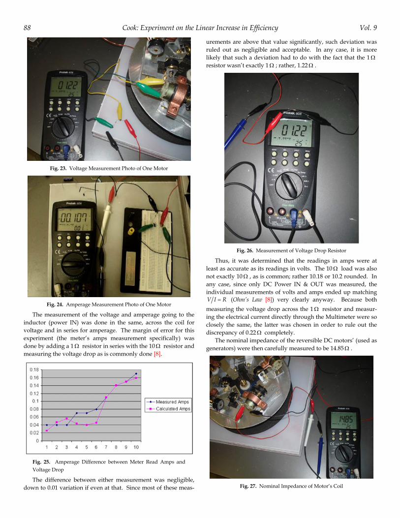
Fig. 23. Voltage Measurement Photo of One Motor

Fig. 24. Amperage Measurement Photo of One Motor

The measurement of the voltage and amperage going to the inductor (power IN) was done in the same, across the coil for voltage and in series for amperage. The margin of error for this experiment (the meter’s amps measurement specifically) was done by adding a 1 resistor in series with the 10 resistor and measuring the voltage drop as is commonly done [8].

Fig. 25. Amperage Difference between Meter Read Amps and Voltage Drop

The difference between either measurement was negligible, down to 0.01 variation if even at that. Since most of these meas-

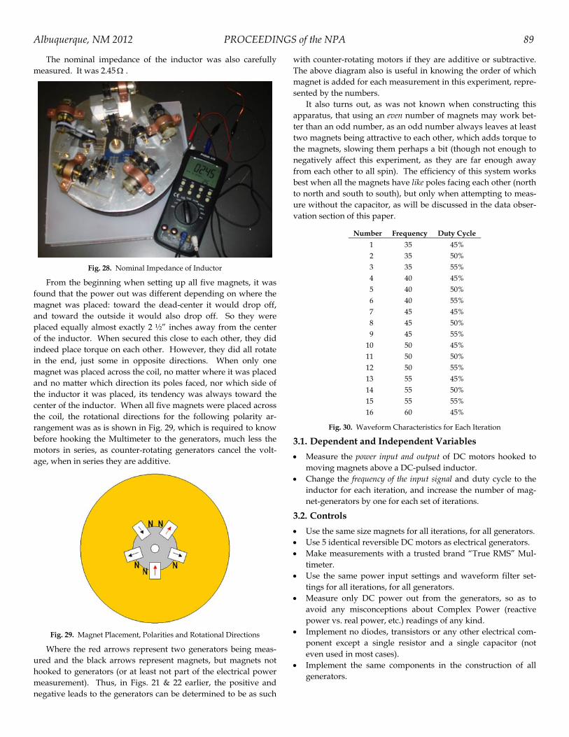
urements are above that value significantly, such deviation was ruled out as negligible and acceptable. In any case, it is more likely that such a deviation had to do with the fact that the 1 resistor wasn’t exactly 1 ; rather, 1.22 .

Fig. 26. Measurement of Voltage Drop Resistor

Thus, it was determined that the readings in amps were at least as accurate as its readings in volts. The 10 load was also not exactly 10 , as is common; rather 10.18 or 10.2 rounded. In any case, since only DC Power IN & OUT was measured, the individual measurements of volts and amps ended up matching V I R (Ohm’s Law [8]) very clearly anyway. Because both

measuring the voltage drop across the 1 resistor and measur-ing the electrical current directly through the Multimeter were so closely the same, the latter was chosen in order to rule out the discrepancy of 0.22 completely.

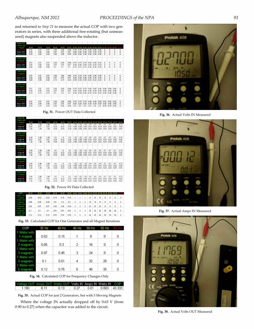
The nominal impedance of the reversible DC motors’ (used as generators) were then carefully measured to be 14.85 .

Fig. 27. Nominal Impedance of Motor’s Coil


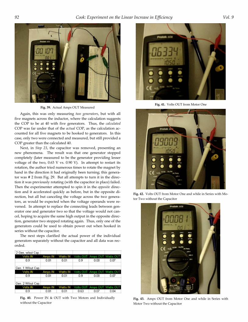
The nominal impedance of the inductor was also carefully measured. It was 2.45 .

Fig. 28. Nominal Impedance of Inductor

From the beginning when setting up all five magnets, it was found that the power out was different depending on where the magnet was placed: toward the dead-center it would drop off, and toward the outside it would also drop off. So they were placed equally almost exactly 2 ½” inches away from the center of the inductor. When secured this close to each other, they did indeed place torque on each other. However, they did all rotate in the end, just some in opposite directions. When only one magnet was placed across the coil, no matter where it was placed and no matter which direction its poles faced, nor which side of the inductor it was placed, its tendency was always toward the center of the inductor. When all five magnets were placed across the coil, the rotational directions for the following polarity ar-rangement was as is shown in Fig. 29, which is required to know before hooking the Multimeter to the generators, much less the motors in series, as counter-rotating generators cancel the volt-age, when in series they are additive.

Fig. 29. Magnet Placement, Polarities and Rotational Directions

Where the red arrows represent two generators being meas-ured and the black arrows represent magnets, but magnets not hooked to generators (or at least not part of the electrical power measurement). Thus, in Figs. 21 & 22 earlier, the positive and negative leads to the generators can be determined to be as such

with counter-rotating motors if they are additive or subtractive. The above diagram also is useful in knowing the order of which magnet is added for each measurement in this experiment, repre-sented by the numbers.

It also turns out, as was not known when constructing this apparatus, that using an even number of magnets may work bet-ter than an odd number, as an odd number always leaves at least two magnets being attractive to each other, which adds torque to the magnets, slowing them perhaps a bit (though not enough to negatively affect this experiment, as they are far enough away from each other to all spin). The efficiency of this system works best when all the magnets have like poles facing each other (north to north and south to south), but only when attempting to meas-ure without the capacitor, as will be discussed in the data obser-vation section of this paper.

Number Frequency Duty Cycle

1 35 45% 2 35 50% 3 35 55% 4 40 45% 5 40 50% 6 40 55% 7 45 45% 8 45 50% 9 45 55% 10 50 45% 11 50 50% 12 50 55% 13 55 45% 14 55 50% 15 55 55% 16 60 45%

Fig. 30. Waveform Characteristics for Each Iteration

3.1. Dependent and Independent Variables

Measure the power input and output of DC motors hooked to moving magnets above a DC-pulsed inductor.

Change the frequency of the input signal and duty cycle to the inductor for each iteration, and increase the number of mag-net-generators by one for each set of iterations.

3.2. Controls

Use the same size magnets for all iterations, for all generators. Use 5 identical reversible DC motors as electrical generators. Make measurements with a trusted brand “True RMS” Mul-

timeter. Use the same power input settings and waveform filter set-

tings for all iterations, for all generators. Measure only DC power out from the generators, so as to

avoid any misconceptions about Complex Power (reactive power vs. real power, etc.) readings of any kind.

Implement no diodes, transistors or any other electrical com-ponent except a single resistor and a single capacitor (not even used in most cases).

Implement the same components in the construction of all generators.


Filter any waveform frequencies and overtones sent to the inductor above 70 Hz in order to restrict the measurements to the range of the experiment (35-55 Hz).

Implement three different duty cycles (45%, 50% & 55%) for each signal frequency in order to better rule in or out positive or negative factors resulting from such variations, such as feedback or the similar from the inductor to the amplifier (re-active power, AKA imaginary power).

The DC generator outputs are in no way hooked to the input electrical circuit, completely independent circuits.

No additional power sources (battery, etc.) or springs are im-plemented.

Operate the reversible DC motors far below their ratings (½ - 1½ V for a 9-18V rating) in order to dramatically decrease their efficiency in order to better measure significant increases in efficiency (DC motors are at best around 80% efficient to begin, reversing them in order to use them as generators de-creases their efficiency further and using them below their rating decreases their efficiency even more).

Operate all frequencies sent to the coil below the wall AC frequency (60Hz) in order to eliminate any potential resonant factors.

Implement no change in mechanical advantage from the magnet diameter to the motor axle (both have an equal diam-eters), but do implement a belt connecting the two.

Do not touch the amplifier power during the experiments; rather, decrease beforehand with filter settings so that the Power IN decreases with an increase in frequency.

4. Assumptions

A DC-pulsed magnetic field in the presence of an external permanent magnet creates an “open mechanical system”, as any linear increase in efficiency would be impossible for a closed system due to the law of conservation of energy, and therefore would prevent my hypothesis from having any va-lidity to begin with.

Additional energy driving any increase in efficiency for an open system comes from the Vacuum Field energy of space (how it could do this is not part of the assumption), as energy is never created or destroyed (it must come from somewhere).

The Multimeter is at least accurate to 0.00(1) readings, as all

values are rounded to th1 100 (0.01).

5. Experimental Steps

5.1. First Phase

1. Turn on the amplifier, computer and Multimeter. 2. Prepare to measure the Voltage IN first with one magnet

hooked to the apparatus, referring to Fig. 21 (but with only one generator to begin and without the capacitor).

3. Generate the waveform for the iteration, using Fig. 30 and send the signal to the amplifier (press PLAY in the audio software application).

4. Measure the voltage across the inductor and record the meas-urement in a datasheet.

5. Repeat steps 3 & 4 for all waveforms in Fig. 30. 6. Prepare to measure the Amperage IN next referring to Fig. 22.

7. Generate the waveform for the iteration, using Fig. 30 and send the signal to the amplifier (press PLAY in the audio software application).

8. Measure the Amperage in series with the inductor and record the measurement in a datasheet.

9. Repeat steps 7 & 8 for all waveforms in Fig. 30. 10. Prepare to measure the Voltage OUT referring to Fig. 21. 11. Generate the waveform for the iteration, using Fig. 30 and

send the signal to the amplifier (press PLAY in the audio software application).

12. Measure the Voltage across the 10 load resistor and record the measurement in a datasheet and record the measurement in a datasheet.

13. Repeat steps 3 & 4 for all waveforms in Fig. 30. 14. Prepare to measure the Amperage OUT referring to Fig. 22. 15. Generate the waveform for the iteration, using Fig. 30 and

send the signal to the amplifier (press PLAY in the audio software application).

16. Measure the Amperage in series with the 10 load resistor and record the measurement in a datasheet.

17. Repeat steps 15 & 16 for all waveforms in Fig. 30. 18. Next hook a second magnet to the second generator as shown in

Fig. 29 (the collars can be unscrewed to easily detach (and re-attach) the magnets and belts from the motors, but do not hook the belt to magnet two. This measurement is only to de-termine if adding additional motors reduces or changes the Power IN or Power OUT, as the next steps involve the measurement of only one generator, not the generators in series.

19. Repeat steps 2 through 18, adding a new magnet each time until all iterations are completed for five magnets with one attached to one belt and one generator (takes roughly two to three hours for all iterations).

20. Multiply the number of magnets times the value of each Pow-er OUT, calculate the power OUT and power IN (Power VoltageCurrent) and determine which iteration has the greatest COP (COP Power Out / Power IN).

5.2. Second Phase

21. Referring then to Fig. 29, hook the two red generators in series and introduce the capacitor to the circuit as shown in Figs. 21 & 22. Using the waveform with the greatest COP (remove if necessary any additional magnets, if a COP was obtained greater using four or fewer magnets than was measured with five magnets).

22. Measure the Power IN and Power OUT and COP as before. 23. Remove the capacitor to measure Power IN and Power OUT. 24. Detach the motors in series and measure their individual

power.

6. Data Collection

It was immediately clear that the duty cycle had no affect on either the power IN or power OUT, so the data was copied to a new datasheet that only included the values of the frequencies with a duty cycle of 50%, as shown in Fig. 34.

Having five magnets provided a calculated COP of 40 when multiplying the number of moving magnets by the generated power out of one generator when the inductor is DC pulsed at 50 Hz. So the author prepared the actual COP measurement for that setup,


and returned to Step 21 to measure the actual COP with two gen-erators in series, with three additional free-rotating (but unmeas-ured) magnets also suspended above the inductor.

Fig. 31. Power OUT Data Collected

Fig. 32. Power IN Data Collected

Fig. 33. Calculated COP for One Generator and all Magnet Iterations

Fig. 34. Calculated COP for Frequency Changes Only

Fig. 35. Actual COP for just 2 Generators, but with 5 Moving Magnets

Where the voltage IN actually dropped off by 0.63 V (from 0.90 to 0.27) when the capacitor was added to the circuit.

Fig. 36. Actual Volts IN Measured

Fig. 37. Actual Amps IN Measured

Fig. 38. Actual Volts OUT Measured


Fig. 39. Actual Amps OUT Measured

Again, this was only measuring two generators, but with all five magnets across the inductor, where the calculation suggests the COP to be at 40 with five generators. Thus, the calculated COP was far under that of the actual COP, as the calculation ac-counted for all five magnets to be hooked to generators. In this case, only two were connected and measured, but still provided a COP greater than the calculated 40.

Next, in Step 23, the capacitor was removed, presenting an new phenomena. The result was that one generator stopped completely (later measured to be the generator providing lesser voltage of the two, 0.63 V vs. 0.90 V). In attempt to restart its rotation, the author tried numerous times to rotate the magnet by hand in the direction it had originally been turning; this genera-tor was # 2 from Fig. 29. But all attempts to turn it in the direc-tion it was previously rotating (with the capacitor in place) failed. Then the experimenter attempted to spin it in the opposite direc-tion and it accelerated quickly as before, but in the opposite di-rection, but all but canceling the voltage across the two genera-tors, as would be expected when the voltage operands were re-versed. In attempt to replace the connecting leads between gen-erator one and generator two so that the voltage would not can-cel, hoping to acquire the same high output in the opposite direc-tion, generator two stopped rotating again. Thus, only one of the generators could be used to obtain power out when hooked in series without the capacitor.

The next steps clarified the actual power of the individual generators separately without the capacitor and all data was rec-orded.

Fig. 40. Power IN & OUT with Two Motors and Individually without the Capacitor

Fig. 41. Volts OUT from Motor One

Fig. 42. Volts OUT from Motor One and while in Series with Mo-tor Two without the Capacitor

Fig. 43. Amps OUT from Motor One and while in Series with Motor Two without the Capacitor


While both motors alone produced an actual COP of greater than one, together in series, however, they were unable to add their respective powers without the capacitor in the circuit. And when applying the capacitor across the two generators in series, the input voltage (Voltage IN to the inductor) was reduced by the exact magnitude of the second generator’s voltage (0.63 V), even though the generators were in no way connected to the inductor circuit.

7. Data Analysis

The actual (real) power OUT was greater than the actual (real) power IN, as the calculations derived from the first phase of the experiment suggested it should. However, the calculation sug-gested that the addition of new magnets in succession should increase linearly. For the following graphs in this analysis, show-ing the calculated Power IN vs. Power OUT (necessary to known in order to determine the optimum frequency and setup) the ex-perimenter refers to the numbers and frequencies in the data-sheet in Fig. 44.

Frequency (Hz)

Duty Cycle (%)

35 50 40 50 45 50 50 50 55 50 60 50

Fig. 44. Frequency Table and Duty Cycles

Fig. 45. Power IN vs. Power OUT for 1 Generator with 1 Magnet

Fig. 46. Power IN vs. Calculated Power OUT for 1 Generator with 2 Magnets




Fig. 50. Graph of Actual COP (a.COP) Compared to Calculated COPs with More Magnets


Fig. 51. Graph of Actual COP (a.COP) Compared to Calculated COPs (c.COP) with More Magnets, Compared to Actual COP with Two Series Generators

The capacitor across the two generators in series seemed to reduce the power IN to the inductor by the exact magnitude of the voltage of the additional generator (0.63 V). This would im-ply that the generators are no longer acting as generators affected by the inductor; rather the other way around when a capacitor is across them. Instead, the generators seem to be acting again as motors, rotating the magnets faster and in turn generating cur-rent back to the inductor, thereby reducing its impedance, but canceling much of its voltage. The nominal impedance of the inductor was measured as 2.45 . When the capacitor was out of the circuit, based on the Power IN, the calculated impedance (when pulsed) of the inductor equaled 90 (V I R ). Howev-

er, with the capacitor in the circuit, the impedance of the inductor reduced to 27 , which may suggest an external increase in elec-trical current in the inductor, but with opposite voltage oper-ands, negating much of the power put in, most reasonably in-duced by the moving magnets above it, now “powered” external-ly.

The analysis of the capacitor is somewhat straight forward with these results, though an external ground state of the energy of the system seems to this experimenter as greater than ex-pected. The voltage of the two motors in series without a load and without the capacitor (not discussed further above, but were measured) was roughly the same as it was with the capacitor and the load, though the voltages across the two series generators do not add (0.90 + 0.63 ≠ 1.18 V); the power between the two genera-tors on the other hand does roughly add (0.11 ~ 0.13 Watts). Thus, it seemed to the author that because the flow of charge through the generator side of the circuit tends through the capac-itor (path of least resistance/action) before it passes to the load (in order to charge it) that the capacitor somehow maintains that voltage across the series generators throughout all cycles, even with the same measured current read in series through the load. It seemed to become a self-sustaining system to some degree even though the Power OUT is not passed directly (by means of electrical connections), rather through induction between the magnets and the inductor. In other words, when the power OUT becomes greater than the power IN, the power IN ceases to re-main constant, is reduced farther.

Lastly, while the COP may be greater with or without the ca-pacitor, the reversible induction (the magnets acting back on the inductor itself) does not occur without the capacitor. Without the

addition of the capacitor, as shown in Fig. 32, the power IN is constant no matter how many magnets are suspended above it. It is only when the capacitor is added is the Power IN re-duced/affected by the motions of the magnets.

8. Conclusion

Summary Statement

This experiment did not support my hypothesis that the efficiency would increase linearly in such an apparatus with the addition of each new generator to the system; instead, it increases exponentially.

While the hypothesis stated that I thought the increase in effi-ciency (the COP) would increase linearly with each additional generator, it actually increased exponentially. While the increase in calculated power OUT was nearly linear up to some threshold, as shown in Figs. 45 through 49, the power IN dropped off ex-ponentially due to the filtering reduction of power from the am-plifier and even more so by means of the magnets’ motions, in-ducing an opposite voltage back to the inductor. This suggests to this experimenter that the power IN is not closed with respect to the generators (which is the common understanding [20]) but additionally that the power OUT is not closed with respect to some external field (not the common understanding), as the measurements actually taken for just one generator with one magnet does not drop off with the same input power. Instead it increases in magnitude in relation with an increase in frequency, as if unaffected by the power so long as the power is of enough magnitude to set the magnets in motion.

It seemed to the author, that while the hypothesis was not ex-actly supported (in that the efficiency would increase linearly), the approach to this experiment based on Gauge Theory and the increase in gauge fields (and in return a higher ground state) was still sound, as the increase in efficiency was exponential. The misunderstanding from exponential to linear (and vice versa) perhaps lies in the nature that the fields being added to the in-ductor do not only interact between the magnets and the induc-tor; rather, additionally with other external fields outside the permanent magnets and the inductor. This is most likely certain with the addition of the electric E field across the capacitor when it was added. However, since the COP > 1 even before the addi-tion of the capacitor, it is not the only field adding to the energy ground state. If the magnets added caused a linear growth, then perhaps it would have ruled out any external fields being added other than those present in each permanent magnet added to the system. However, this was not the case.

It is the author’s conclusion based on the lack of support of the hypothesis, but with larger significance and magnitude, that the system’s Zero Point Energy (the sum of the energies of all the fields in the system) was not only increased with the addition of each magnet to the system, but that the Vacuum Energy (the sum of all fields present in space), was also interacted with, as the energy was increased beyond that of the sum of the energies of all the fields in the system. The principle allowing such a conclu-sion is the Principle of Least Action, which arises once the mag-nets are put in motion and are met with a field in the opposite direction before the energy of its motion is fulfilled.

The mechanism is then concluded as such based on this ex-periment:


1. The inductor is pulsed. 2. The magnet suspended above the inductor experiences mo-

tion with high kinetic energy in one direction. 3. The inductor experiences a change/decay in the field, but by

means of inertia (Newton’s First Law of Motion [5], an object put in motion tends to stay in motion), the magnet continues in the same direction for some amount of time > 0.

4. The inductor is pulsed again and the magnet is affected in a different direction before its kinetic energy is fully used com-pletely from the energy of the first pulse (“stored” as poten-tial energy, momentum conserved by potential angular mo-mentum or potential momentum [17]), the resulting turn of the magnet is not directly back and forth unless its angle is re-stricted on a rod, but in this case it is.

5. Since the degree of freedom of movement (the average of all the magnet’s degree of freedom of movement being measured in Kelvin’s) is restricted/limited, by means of the Principle of Least Action [4], the magnet must return in the opposite di-rection (the farthest directional degree from this force being 180 or radians, a change in angular momentum) in order to avoid transversing some space against a greater action and a greater corresponding force, but using the remaining kinetic energy from the previous pulses, which is being added to some potential energy reservoir with every pulse.

6. Since the energy of the back and forth motions are synchro-nous with regular successively timed pulses, the extra stored potential energy being added with each cycle must be applied somewhere; in this case to movement in a different axis in three dimensions (another change in angular momentum).

7. If allowed to rotate, this unused energy is applied to that mo-tion; however, if the torque against the rotation is too great, the potential energy is supplied in another manner: not only by turning the magnet (a change in angular momentum), but actually vibrating the rod it is on—if the rod is rigid (prevent-ed from vibrating) but with some significant length, then it moves the magnet out of the way (orbit) along this rod, or at least as far as it can (if it meets a barrier, then it simply returns the opposite direction, so long as the energy is being spent somehow).

8. If the potential energy is not released to kinetic energy as fast as the system adds it, then other motions can be obtained; ad-ditional motions (flow) gives rise to additional gauge fields per the Noether Theorem [7].

9. As restricting the angle the magnet precesses at adds to the kinetic energy of the rotation, as well as does restricting the nutation by suspending the ring magnet on the rod, so too does the energy of the rotation increase with a decreased an-gle of which it is permitted to precesses (and a resulting in-crease in angular momentum), and so too does a further re-striction of the direction of orbit (keeping the magnet fixed on a belt, resisting side to side motion).

10. Since the unused potential energy induced on the magnet seems only directly transferable to another field of force after an additional field is created (the energy of the system alone does not supply enough energy to create additional fields, its ground state is not affected to the same magnitude), it seems more likely to the author that the energy supplied to create any additional fields (to change the motion to a different spa-

tial dimension on the X, Y, Z plane, a significant change in angular momentum, remembering that the increase in effi-ciency is greater than linear with this experiment), could be being obtained by Vacuum Energy rather than from the sys-tem’s ground state.

11. If the system were to have an EM resonating factor, it poten-tially could “rob” energy from nearby electrical circuits of the same frequency through resonance [8]; however, no such fac-tor existed at the frequencies used in this experiment (35 Hz to 55 Hz with DC output)—this could also occur hypothetical-ly in terms of temperature (in some sense) [18], but no tem-perature changes were noticed throughout this experiment at all.

12. Placing a purely resistive load on the output does not (and did not) release the unused/potential energy; rather, it in-creases it, as the energy of the magnets is best released by mo-tion (in order to obey the Principle of Least Action [4], to get out of a magnetic repulsive state) and a resistive load would further limit the kinetic energy by slowing the motors—and thus the magnets connected to it (which is most likely why the two generators had a greater COP when placed on the load rather than when they were left free spinning and only calculated).

13. When the cycle repeats faster than the energy can be distrib-uted kinetically, the symmetry of the system becomes “bro-ken” (no longer existing as an algebraic “Lie Group” [1]; ra-ther, a “Topological Group” [2]), thereby “opening” it in or-der to interact with external fields (as well as their energies) in order to obtain more energy to fulfill least action; if this is not possible to the required magnitude, the input power seems (to this experimenter) to be additionally reduced in scenarios where mutual induction is possible (as is in this case with this experiment) with a reversal of the magnet’s rotation, thereby supplying the opposite voltage back to the inductor.

Future experiments that should be produced:

No generators were brought near the bottom or sides of the inductor, but magnets have been shown to move in the same way at those locations (more than just 5 magnets on the top should be experimented with).

Smaller magnets should be experimented with, as they could be brought together closer, having the same field strength

Better constructed apparatuses should be designed, using CNC machining now that initial results have shed light on the effectiveness and behavior of the apparatus.

At some point, an experiment should be constructed with 555 Timers and Op-Amp power transformer circuits run off a bat-tery, where the output could be reapplied to the input.

Additional motions should be sought by restricting rotation and/or precession completely.

References

[ 1 ] John Frank Adams, Lectures on Lie Groups, Chicago Lectures in Mathematics (Chicago: Univ. of Chicago Press, 1969).

[ 2 ] Alexander Arhangel’skii, Mikhail Tkachenko, Topological Groups and Related Structures (Atlantis Press, 2008).


[ 3 ] John Patrick Barrett, “Electricity at the Columbian Exposition; In-cluding an Account of the Exhibit in the Electricity Building, the Power Plant in Machinery Hall” (1894).

[ 4 ] Leonhard Euler, Methodus Inventendi Lineas Curvas Maximi Minive Proprietate Gaudentes (Lausanne & Geneva, 1744); Re-printed in C. Cartheodory, Ed., Leonhardi Euleri Opera Omnia: Series I, Vol. 24 (Orell Fuessli, Zurich, 1952).

[ 5 ] I. Galili, M. Tseitlin, “Newton’s First Law: Text, Translations, In-terpretations and Physical Education”, Science & Education 12 (1): 45-73 (2003).

[ 6 ] David Griffiths, Introduction to Electrodynamics (Prentice-Hall, 1989).

[ 7 ] D. Gross, “Gauge Theory: Past, Present and Future”, Chinese Jour-nal of Physics 30: 7 (1992).

[ 8 ] James H. Harter, Paul Y. Lin Essentials of Electric Circuits (Reston Publishing Co., 1982).

[ 9 ] William Hayt, Engineering Electro-Magnetics, 5th Ed. (McGraw-Hill, New York, 1989).

[ 10 ] http://en.wikipedia.org/wiki/tamtam.

[ 11 ] http://www.aikenamps.org/whatIsBiasing.htm. [ 12 ] http://www.youtube.com/jnoelcook. [ 13 ] K. J. Laidler, The World of Physical Chemistry (Oxford University

Press, 2001). [ 14 ] T. D. Lee, Symmetries, Asymmetries and the World of Particles

(University of Washington Press, Seattle, 1988). [ 15 ] M. Planck, A. Ogg (trans.), Treatise on Thermodynamics (Long-

mans, Green & Co., London, 1897/1903). [ 16 ] Edward M. Purcell, Electricity and Magnetism, Berkeley Physics

Course II (McGraw-Hill, New York, 1965). [ 17 ] David J. Raymond, “Potential Momentum, Gauge Theory, and

Electromagnetism in Introductory Physics”, arXiv:physics/9803023 v1 [physics.ed-ph] (1998).

[ 18 ] F. Reif, Fundamentals of Statistics and Thermal Physics (McGraw Hill, New York, 1965).

[ 19 ] John R. Reitz, Frederick J. Milford; Robert W. Christy, Foundations of Electromagnetic Theory (Addison-Wesley, 1993).

[ 20 ] M. N. O. Sadiku, Elements of Electromagnetics, 4th Ed. (Oxford University Press, 2007).

cook - experiment on the linear increase in efficiency ... · experiment on the linear increase in...

Documents