control systems on lie groups
TRANSCRIPT
Control Systems on
Lie Groups
P.S. Krishnaprasad
Department of Electrical and Computer
Engineering
and
Institute for Systems Research
University of Maryland, College Park, MD
20742
1

Control Systems on Lie Groups
• Control systems with state evolving on a
(matrix) Lie group arise frequently in phys-
ical problems.
• Initial motivation came from the study of
bilinear control systems (control multiplies
state).
• Problems in mechanics with Lie groups as
configuration spaces
2

Example from Curve Theory
Consider a curve γ in 3 dimensions.
γ : [0, tf ] → R3 (1)
where t ∈ [0, tf ] is a parametrization. A classi-
cal problem is to understand the invariants of
such a curve, under arbitrary Euclidean trans-
formations.
First, restrict to regular curves, i.e.,dγ
dt= 0 on
[0, tf ]. Then
s(t) =∫ t0
∣∣∣∣∣∣∣∣dγdt′
∣∣∣∣∣∣∣∣ dt′ (2)
is the arc-length of the segment from 0 to t.
From regularity, one can switch to a parametriza-
tion in terms of s.
3

Example from Curve Theory
speed ν =∣∣∣∣∣∣∣∣dγdt
∣∣∣∣∣∣∣∣ = ds
dt
Tangent vector T = γ′ = dγ
ds=
1
ν
dγ
dtThus s-parametrized curve has unit speed.
If curve is C3 and T ′ = γ′′ = 0 then we canconstruct Frenet-Serret frame T,N,B where
N =T ′
||T ′|| (3)
and
B = T ×N (4)
By hypothesis, curvature κ= ||T ′|| > 0 and
torsion is defined by
τ(s)=γ′(s) · (γ′′(s) × γ′′′(s)
)(κ(s))2
(5)
4

Example from Curve Theory
Corresponding Frenet-Serret differential equa-
tions are
T ′ = κNN ′ = −κT +τBB′ = −τN
(6)
Equivalently
d
ds
[T N B γ0 0 0 1
]
=
[T N B γ0 0 0 1
] ⎡⎢⎢⎢⎣0 −κ 0 1κ 0 −τ 00 τ 0 00 0 0 0
⎤⎥⎥⎥⎦
(7)
5

Example from Curve Theory
6

Example from Curve Theory
There is an alternative, natural way to frame a
curve that only requires γ to be a C2 curve and
does not require γ′′ = 0. This is based on the
idea of a minimally rotating normal field. The
corresponding frame T,M1,M2 is governed
by:
T ′ = k1M1 + k2M2
M ′1 = −k1T (8)
M ′2 = −k2T
Here k1(s) and k2(s) are the natural curvature
functions and can take any sign.
7

Frame Equations and Control
The natural frame equations can be viewed
as a control system on the special Euclidean
group SE(3):
d
ds
[T M1 M2 γ0 0 0 1
]
=
[T M1 M2 γ0 0 0 1
] ⎡⎢⎢⎢⎣0 −k1 −k2 1k1 0 0 0k2 0 0 00 0 0 0
⎤⎥⎥⎥⎦
(9)
Here, g the state in SE(3) evolves under con-
trols k1(s), k2(s). The problem of growing a
curve is simply the problem of choosing the
curvature functions (controls) k1(·), k2(·) over
the interval [0, L] where L = total length. Ini-
tial conditions are needed.
8

Frame Equations and Control
It is possible to write everything in terms of
the non-unit speed parametrization t. In that
case,
dg
dt= νgξ (10)
where ν is the speed and,
ξ =
⎡⎢⎢⎢⎣
0 −k1 −k2 1k1 0 0 0k2 0 0 00 0 0 0
⎤⎥⎥⎥⎦ (11)
Here ξ(·) is a curve in the Lie algebra se(3) of
the group SE(3), i.e., the tangent space at the
identity element of SE(3).
ν(·), k1(·) and k2(·) are controls.
9

Examples Related to Curve Theory
• control of a unicycle can be modeled as a
control problem on SE(2).
• Control of a particle in R2 subject to gyro-
scopic forces can be modeled as a control
problem on SE(2).
10

Left-invariant Control Systems on Lie
Groups
G is a Lie group with Lie algebra g.
Lg : G→ G Rg : G→ G
h→ gh h→ hg
Lg is left translation and Rg is right translation.
Control system
g = TeLg · ξ (12)
where ξ(·) is a curve in the Lie algebra. For
matrix Lie groups this takes the form
P = PX (13)
11

Left-invariant Control Systems on Lie
Groups
Explicitly, let ξ0, ξ1, ..., ξm be fixed elements in
g. Consider
ξ(t) = ξ0 +m∑i=1
ui · ξi (14)
where ui(·) are control inputs. Then (12) (and
(13)) is manifestly a left invariant system:
Lhg = TeLhg
= TeLhTeLgξ
= TeLhgξ
= Te(Lhg)ξ
12

Left-invariant Control systems on Lie
Groups, cont’d
Input-to-state response can be written locally
in t as
g(t) = exp (ψ1(t)ξ1) exp (ψ2(t)ξ2)...exp (ψn(t)ξn)g0
where ψi are governed by Wei-Norman differ-
ential equations driven by ui and ξ1, ..., ξn is
a basis for g.
13
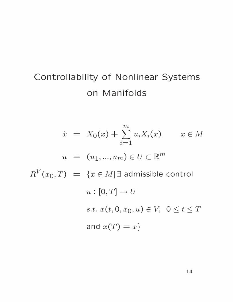
Controllability of Nonlinear Systems
on Manifolds
x = X0(x) +m∑i=1
uiXi(x) x ∈M
u = (u1, ..., um) ∈ U ⊂ Rm
RV (x0, T) = x ∈M | ∃ admissible control
u : [0, T ] → U
s.t. x(t,0, x0, u) ∈ V, 0 ≤ t ≤ T
and x(T) = x
14
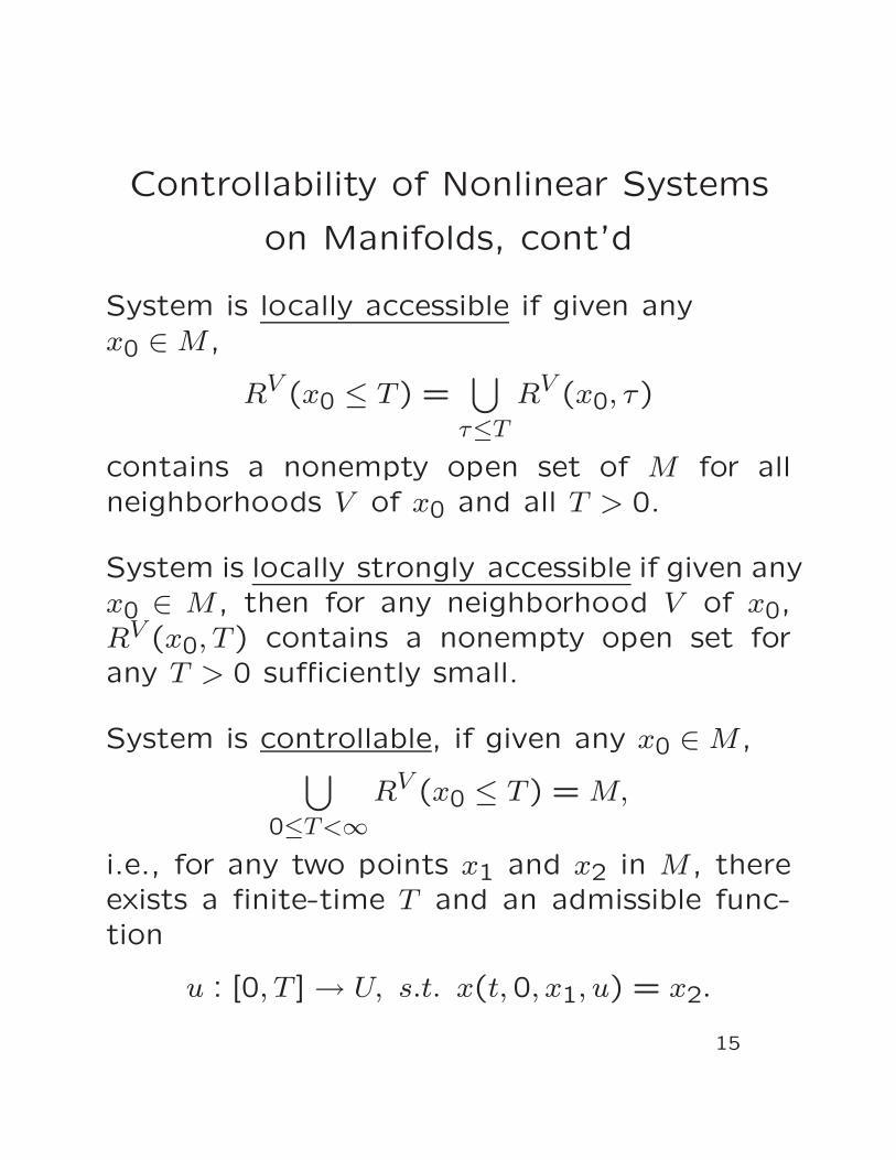
Controllability of Nonlinear Systems
on Manifolds, cont’d
System is locally accessible if given anyx0 ∈M ,
RV (x0 ≤ T) =⋃τ≤T
RV (x0, τ)
contains a nonempty open set of M for allneighborhoods V of x0 and all T > 0.
System is locally strongly accessible if given anyx0 ∈ M , then for any neighborhood V of x0,RV (x0, T) contains a nonempty open set forany T > 0 sufficiently small.
System is controllable, if given any x0 ∈M ,⋃0≤T<∞
RV (x0 ≤ T) = M,
i.e., for any two points x1 and x2 in M , thereexists a finite-time T and an admissible func-tion
u : [0, T ] → U, s.t. x(t,0, x1, u) = x2.
15

Controllability of Nonlinear Systems
on Manifolds
Let L = smallest Lie subalgebra of the Lie
algebra of vector fields on M that contains
X0, X1, ...,Xm. We call this the accessibility
Lie algebra.
Let L(x) = span X(x)|X vector field inL.
Let L0 = smallest Lie subalgebra of vector
fields on M that contains X1, ..., Xm and satis-
fies [X0, X] ∈ L0 ∀ X ∈ L0.
Let L0(x) = span X(x)|X vector field in L0.
16

Controllability of Nonlinear Systems
on Manifolds, cont’d
Local accessibility
↔ dimL(x) = n,∀x ∈M. (LARC)
Local strong accessiblity ↔ dimL0(x) = n,
∀x ∈M.
Local accessiblity + X0 = 0 ⇒ Controllable
(Chow)
17

Controllability on Groups
Consider the system∑
given by (12), (13).
(i) We say∑
is accessible from g0 if there ex-ists T > 0 such that for each t ∈ (0, T),the set of points reachable in time ≤ t hasnon-empty interior.
(ii) We say∑
is controllable from g0 if for eachg ∈ G, there exists a T > 0 and a con-trolled trajectory γ such that γ(0) = g0and γ(T) = g.
(iii) We say∑
is small time locally controllable(STLC) from g0 ∈ G if there exists a T > 0such that for each t ∈ (0, T), g0 belongs tothe interior of the set of points reachablein time ≤ t.
18

Controllability on Lie Groups
Let U = admissible controls be either
Uu, Uγ, or Ub,where
(i) Uu = class of bounded measurable func-
tions on [0,∞] with values in Rm.
(ii) Uγ = subset of U taking values in unit n-
dimensional cube.
(iii) Ub = subset of U with components piece-
wise constant with values in −1,1.
19

Controllability on Lie Groups, cont’d
Theorem (Jurdjevic–Sussmann, 1972)
If ξ0 = 0, then controllable with u ∈ Uiff ξ1, ..., ξmL.A. = g. If U = Uu then
controllable in arbitrarily short time.
Theorem (Jurdjevic-Sussman, 1972).
G compact and connected.
Controllable if ξ0, ξ1, ..., ξmL.A. = g.
There is a bound on transfer time.
Semisimple ⇒ tight bound.
20

Constructive Controllability
Underactuated systems:
m < dim (G)
Can we get yaw out of pitch and roll? Yes –
exploit non-commutativity of SO(3).
Specific idea: If drift-free, then oscillatory,
small amplitude controls together with an ap-
plication of averaging theory yields area rule
and constructive techniques.
R.W. Brockett (1989), Sensors and Actu-
ators, 20(1-2): 91-96.
N.E. Leonard (1994), Ph.D. thesis, Univer-
sity of Maryland
21

N.E. Leonard and P.S. Krishnaprasad (1995),
IEEE Trans. Aut. Contrl, 50(9): 1539-
1554.
R.M. Murray and S. Sastry (1993), IEEE
Trans. Aut. contrl, 38(5):700-716

Mechanical Systems on Lie Groups
– Lie groups as configuration spaces of clas-sical mechanical systems.
– Lagrangian mechanics on TG.
– Hamiltonian mechanics on T ∗G.
Key finite dimensional examples:
(a) The rigid body with Lagrangian
L =1
2Ω · IΩ − V
where
Ω = body angular velocity
vector ∈ R3
I = moment of inertia tensor
22

Mechanical Systems on Lie Groups,
cont’d
(Here, body has one fixed point.)
For heavy top, potential V = −mg ·Rχ where
χ = body-fixed vector from point of
suspension to center of mass.
g = gravity vector.
23
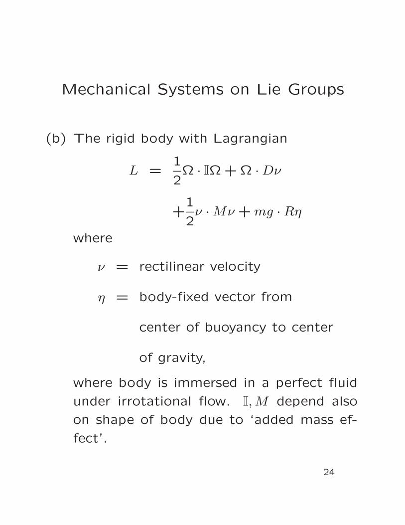
Mechanical Systems on Lie Groups
(b) The rigid body with Lagrangian
L =1
2Ω · IΩ + Ω ·Dν
+1
2ν ·Mν +mg ·Rη
where
ν = rectilinear velocity
η = body-fixed vector from
center of buoyancy to center
of gravity,
where body is immersed in a perfect fluid
under irrotational flow. I,M depend also
on shape of body due to ‘added mass ef-
fect’.
24

Mechanical Systems on Lie Groups
Garret Birkhoff was perhaps the first to dis-
cuss the body-in-fluid problem as a system on
the Lie group SE(3). (See HASILFAS, 2nd
edition, (1960), Princeton U. Press).
25

Controlled Mechanical Systems on Lie
Groups
Hovercraft (planar rigid body with vectored
thruster)
P1 = P2Π/I + αu
P2 = −P1Π/I + βu
Π = dβu
R = RΠ
I; Π =
(0 −11 0
)Π
r = RP
m; R = Rot(θ)
Observe that the first three equations involve
neither R nor r.
26
Controlled Mechanical Systems on Lie
Groups, cont’d
This permits reduction to the first three, a
consequence of SE(2) symmetry of the planar
rigid body Lagrangian and the “follower load”
aspect of the applied thrust.
Related work by N. Leonard, students and col-
laborators.
27

Controllability of Mechanical Systems
on Lie Groups
In general, on T ∗G, Xo = 0. We need the idea
of Poisson Stability of drift.
X is smooth complete vector field on M .
φXt is flow of X.
p ∈ M is positively Poisson stable for X if for
all T > 0 and any neighborhood Vp of p, there
exists a time t > T such that
φXt (p) ∈ Vp.
X is called positively Poisson stable if the set
of Poisson stable points of X is dense in M .
28

Controllability of Mechanical Systems
on Lie Groups
A point p ∈ M is a non-wandering point of X
if for any T > 0 and any neighborhood Vp of p,
there exists a time t > T such that
φXt (Vp) ∩ Vp = ∅
X is Poisson stable ⇒ nonwandering set = M .
X is WPPS if nonwandering set of X is M .
29
Controllability of Mechanical Systems
on Lie Groups
Theorem (Lian, Wang, Fu, 1994):
Control set U contains a ‘rectangle’.
X0 is WPPS.
Then, LARC ⇒ Controllability
Poincare recurrence theorem
⇒ time independent Hamiltonian vector field
on a bounded symplectic manifold isWPPS.
30

Controllability of Mechanical Systems
on Lie Groups, cont’d
Theorem (Manikonda, Krishnaprasad, 2002):
Let G be a Lie group and H : T ∗G→ R
a left-invariant Hamiltonian.
(i) If G is compact, the coadjoint orbits ofg∗ = T ∗G/G are bounded and Lie-Poissonreduced dynamics XH is WPPS.
(ii) If G is noncompact, then the Lie-Poissonreduced dynamics is WPPS if there exists afunction V : g∗ → R such that V is boundedbelow and V (µ) → ∞, as ||µ|| → ∞ andV = 0 along trajectories of the system.
Here H is the induced Hamiltonian on the quo-tient manifold g∗ = T ∗G/G.
31

Controllability of Mechanical Systems
on Lie Groups, cont’d
Controllability of reduced, controlled dynamics
on g∗ is of interest and can be inferred in vari-
ous cases by appealing to the above theorems
of (Lian, Wang and Fu, 1994) and (Manikonda
and Krishnaprasad, 2002).
This leaves unanswered the question of con-
trollability of the full dynamics on T ∗G. To
sort this out, we need WPPS on T ∗G.
32

Controllability of Mechanical Systems
on Lie Groups
Theorem (Manikonda and Krishnaprasad, 2002):
Let G be a compact Lie group whose Poisson
action on a Poisson manifold M is free and
proper. A G-invariant hamiltonian vector field
XH defined on M is WPPS if there exists a
function V : M/G→ R that is proper, bounded
below, and V = 0 along trajectories of the pro-
jected vector field XH defined on M/G.
To use this result, we see whether LARC holds
on M . Then appealing to theorem above, if we
can conclude WPPS of the drift vector field
XH then controllability on M holds.
33

Controllability of Mechanical Systms
on Lie Groups, cont’d
Note:
For hovercraft and underwater vehicles,
G is not compact, but a semidirect prod-
uct. See Manikonda and Krishnaprasad,
(2002), Automatica 38: 1837-1850.
34

Controllability of Mechanical Systems
on Lie Groups
Definition:
H = kinetic energy.
Thus g = TeLg(I−1µ)
µ = Λ(µ)∇H +m∑i=1
uifi
Here Λ(µ) = Poisson tensor on g∗.H : g∗ → R given by
H∗(µ) =1
2µ · I
−1µ
I : g → g∗ inertia tensor.
We say that the system is equilibrium control-
lable if for any (g1,0) and (g2,0) there exists a
time T > 0 and an admissible control35

Controllability of Mechanical System
on Lie Groups, cont’d
u : [0, t] → U
such that the solution
(g(t), µ(t))
satisfies
(g(0), µ(0)) = (g1,0) and
(g(T), µ(T)) = (g2,0)
This concept was introduced by Lewis and Mur-
ray (1996).
36

Controllability of Mechanical Systems
on Lie Groups
Theorem (Manikonda and Krishnaprasad, 2002):
The mechanical system on T ∗G with kinetic
energy hamiltonian is controllable if
(i) the system is equlibrium controllable, and
(ii) the reduced dynamics on g∗ is controllable
37

Variational Problems on Lie Groups
Any smooth curve g(·) on a Lie group can be
written as
g(t) = TeLgξ(t)
where ξ(t) = curve in Lie algebra g defined by
ξ(t) =(TeLg(t)
)−1g(t)
Given a function l on g one obtains a left in-
variant Lagrangian L on TG by left translation.
Conversely, given a left-invariant Lagrangian
on TG, there is a function l : g → R obtained
by restricting L to the tangent space at iden-
tity.
38

Variational Problems on Lie Groups,
cont’d
With these meanings for ξ, L, l we state:
Theorem(Bloch, Krishnaprasad, Marsden, Ratiu,
1996):
The following are equivalent:
(i) g(t) satisfies the Euler Lagrange equations
for L on TG.
(ii) The variational principle
δ∫ baL(g(t), g(t)) = 0
holds, for variations with fixed end-points.
39

(iii) The Euler-Poincare equations hold:
d
dt
δl
δξ= ad∗ξ
δl
δξ
(iv) The variational principle
δ∫ bal(ξ(t))dt = 0
holds on g, using variations of the form
δξ = η+ [ξ, η]
where η vanishes at end-points.

Remark: In coordinates
d
dt
∂l
∂ξd= Cbad
∂l
∂ξbξa
where Cbad are structure constants of g relative
to a given basis, and ξa are the components of
ξ relative to this basis.
Remark: Let µ =∂l
∂ξ;
Let h(µ) =< µ, ξ > −l(ξ) be the Legendre trans-
form,
and assume that ξ → µ is a diffeomorphism.
Thendµ
dt= ad∗δh/δµµ
the Lie-Poisson equations on g∗.
These are equivalent to the Euler-Poincare equa-
tions.40

Optimal Control for Left-Invariant
Systems
Consider the control system
g = TeLgξu
where each control u(.) determines a curveξu(.) ⊂ g. Here we limit ourselves to
ξu(t) = ξ0 +m∑i=1
ui(t)ξi
whereξ0, ξ1, ..., ξm+1
spans an m-dimensional
subspace h of g.m+ 1 ≤ n = dim G = dim g.
Consider an optimal control problem
minu(.)
∫ T0L(u)dt
subject to the condition that u(·) steers thecontrol system from g0 at 0 to g1 at T . Ingeneral, T may be fixed or free.
41

Optimal Control for Left-Invariant
Systems
Here we fix T . Clearly, the Lagrangian L is G-
invariant.
It is the content of the maximum principle that
optimal curves in G are base integral curves of
a hamiltonian vector field on T ∗G. To be more
precise, let τG : TG → G and τ∗g : T ∗G → G be
bundle projections.
Define
Hλ = Hλ(αg, u)
= −λL(u)+ < αg, TeLg · ξu >where λ = 1 or 0, and αg ∈ T ∗G.
42

Maximum Principle:
Let uopt be a minimizer of the cost functional
and let g(.) be the corresponding state trajec-
tory in G. Then, g(t) = τ∗G(αg(t)) for an in-
tegral curve αg of the hamiltonian vector field
XuoptHλ
defined for t ∈ [0, T ] such that:
Optimal Control for Left-invariant
Systems, cont’d
(a) If λ = 0 than αg is not the zero section of
T ∗G on [0, T ].
(b) Hλ(αg, uopt) = supu∈U
Hλ(αg, u) for t almost ev-
erywhere in [0, T ]. Here U = space of val-
ues of controls. (We consider U = Rm be-
low.)
(c) If the terminal T is fixed then Hλ(αg, uopt) =
constant and if T is free, then Hλ(αg, uopt) =
0 ∀t ∈ [0, T ]. Trajectories corresponding
to λ = 0 are called abnormal extremals and
they occur but can be ruled out by suitable
hypotheses. We stick to the setting of reg-
ular extremals (λ = 1).
43

Optimal Control for Left-invariant
Systems, cont’d
We calculate the first order necessary condi-
tions:
− ∂L
∂ui+
∂
∂ui< αg, TeLgξu >= 0 i = 1,2, ...,m,
But
< αg, TeLgξu > = < αg, TeLg
⎛⎝ξ0 +
m∑i=1
uiξi
⎞⎠ >
= < TeL∗gαg, ξ0 +
m∑i=1
uiξi >
= < µ, ξ0 > +m∑i=1
ui < µ, ξi >
Thus
− ∂L
∂ui+ < µ, ξi >= 0 i = 1,2, ...,m
44

Optimal Control for Left-invariant
Systems, cont’d
At this stage, the idea is to solve for ui and
plug into
Hλ = −L(u)+ < µ, ξ0 > +m∑i=1
ui < µ, ξi >
to get a G-invariant hamiltonian which descends
to a hamiltonian h on g∗.
45

Optimal Control for Left-invariant
Systems, cont’d
In the special case
L(u) =1
2
m∑i=1
Iiu2i ,
we get ui =< µ, ξi >
Ii
and h =< µ, ξ0 > +1
2
m∑i=1
< µ, ξi >2
Ii.
One solves the Lie-Poisson equation
dµ
dt= ad∗δh/δµµ
to obtain µ as a function of t.Then substitute back into
ui =< µ, ξi >
Ii
to get controls that satisfy first order necessaryconditions.
46

Optimal Control for Left-invariant
Systems, cont’d
Integrable Example (unicycle) on SE(2)
g = g (ξ1u1 + ξ2u2)
where ξ1 =
⎛⎜⎝ 0 −1 0
1 0 00 0 0
⎞⎟⎠
ξ2 =
⎛⎜⎝ 0 0 1
0 0 00 0 0
⎞⎟⎠
L(u) =1
2(u2
1 + u22)
47

Then
h(µ) =1
2(µ2
1 + µ22)
µ1 = −µ2µ3
µ2 = µ1µ3
µ3 = −µ1µ2
Invariants
c = µ22 + µ2
3 (casimir)
h = (µ21 + µ2
2)/2 (hamiltonian)

Optimal Control for Left-invariant
Systems, cont’d
Then
µ2 + (2h+ c)µ2 − 2µ32 = 0
(anharmonic oscillator)
µ2(t) = βSn(γ(t− t0), k)
where Sn(u, k) is Jacobi’s elliptic sine function,
γ s.t.
γ2 < (2h+ c) < 2γ2
t0 is arbitrary and
k2 =2h+ c
γ2− 1
β2 = 2h+ c− γ2
48

Then
µ1 =√
2h− µ22
µ3 =√c− µ2
2
u1 = µ1
and u2 = µ2.

Optimal Control for Left-invariant
Systems
In the above example one can show that there
are no abnormal extremals.
This example is prototypical of a collection of
integrable cases. Where integrability does not
hold, one can still investigate the Lie-Poisson
equations numerically.
49