Consumption, Fiscal Policy and Endogenous Growth:

The Case of India

by

Ila Patnaik

A thesis submitted to the University of Surrey for the Degree of Doctor

of Philosophy in the Department of Economics

November 1995

Abstract

A Structural Adjustment Programme is typically accompanied by fiscal policy

changes aimed at reducing government spending and budget deficits as in India in

recent years. The objective of this thesis is to analyse the impact of these changes on

the economy. Since the eventual disengagement of indebted countries from

international lending agencies like the RV1F and the World Bank has been seen to come

with econon-uc growth which is one of the objectives of the SAP, and as small

differences in the long-run growth rate have a significant impact on standards of living,

our focus is on the effect of government spending policies on the long-run steady state

growth rate. We present an endogenous growth model in which the impact of fiscal

policy is through non-Ricardian effects on the demand side and externalities arising

from public capital on the supply side.

Preliminary results suggest that the Indian economy is non-Ricardian. An

aggregate consumption function that incorporates finite horizons, population growth,

liquidity constraints and tax distortions is estimated investigate non-Ricardian effects

on demand. With supply side parameters that are observed or imposed, the model is

calibrated to examine the impact of changes in the debt/GDP ratio, the tax rate and the

share of development expenditure in total goverrunent spending. Simulations suggest a

very strong positive impact of public investment on the long-run growth rate. At the

same time our analysis shows that non-Ricardian demand side effects though present,

have only a marginal effect on our empirical analysis. The major policy implication that

emerges from our results is that the present trend of a decline in the proportion of

development spending is counter-productive to the objective of growth. A clear

definition of the role of public investment and an analysis of the impact of the

components of public expenditure is essential for a successful SAP.

DECLARATION OF ORIGINALITY

1, Ila Patnaik, hereby declare that the material contained in this dissertation is, to the best of my knowledge, original.

Signed

Dated o-v

fNTER-LIBRARY DECLARATION

1, Ila Patnaik, hereby declare that the material contained in this dissertation may be

made available for photocopying and for inter-library loan.

Signed J',

9-AJ-Jý

Dated I S- N-&-V I ý-

Acknowledgments

I would like to express my deepest gratitude to my supervisor Prof Paul Levine

from whom I received invaluable insights, ideas, guidance and encouragement throughout

the duration of my research. I would also like to thank Prof Wojceich Charemza of the

University of Leicester for his suggestions for my empirical work. I am grateful for the

financial support I received from the British Council and from the Department of

Econon-ýcs, University of Surrey. I would also like to acknowledge the help I received

from staff of the National Council for Applied Economic Research and the National

Institute of Public Finance and Policy, New Delhi.

I am grateful for comments and criticisms offered by friends and colleagues

especially Fotis Mouzakis and Thomas Krichel. And finally, I am indebted to my husband

Ajay, without whose support this work would not have been possible.

Contents

Acknowledgment

Table of notations i-iii

Introduction 1-7

Chapter 1 8-29

Public Spending and Debt in India

1.1. Development Strategy 9

1.2. Financing Development 13

1.3. Growth of Public Expenditure 14

1.4. Tax Revenue 16

1.5. Growth of Public Debt 18

1.6. The External Crisis 20

1.7. Stabilisation and Structural Adjustment 21

1.8. Cut in Development Expenditure 24

Chapter 2 29-46

Debt Neutrality: Theory and Evidence

2.1. A Representative Agent model 30

2.2. The Ricardian Equivalence Hypothesis 34

2.3. Empirical Studies 37

2.4. Excess Sensitivity 42

2.5. Evidence for India 44

Chapter 3 47-57

The Aggregate Consumption Function: Finite Horizons, Liquidity

Constraints and Population Growth with Income Redistribution

3.1. Liquidity Constraints 47

3.2. Finite Horizons 48

3.3. Population Growth and Income Redistribution 49

3.4. Utifity Function 51

3.5. Aggregate Behaviour 54

Chapter 4 58-82

Estimation and Results

4.1. Eliminating Human and Non-human Wealth 58

4.2. Non-Lineanty 60

4.3. Properties of the Disturbance Term 61

4.4. Generalised Method of Moments 64

4.5. Approaches to Estimation 68

4.6. Data 69

4.7. Restrictions 71

4.8. Estimation and Results 72

4.9. Supporting Evidence 75

Chapter 5 83-126

Policy Evaluation in an Endogenous Growth Model

5.1. Traditional Models of Growth 84

5.2. Endogenous Growth 85

5.3. The Model 87

5.3.1. Households 88

5.3.2. Private Sector Output and Investment. 90

5.3.3. The Government 92

5.3.4. Output Equilibrium. 93

5.3.5. The Steady-State 93

5.4. Fiscal Policy and Long-Run Growth 96

5.5. Calibration and Estimation for India 101

5.5.1. The Development Expenditure Multiplier 104

5.5.2. The Tax Multiplier 105

5.5.3. The Debt Multiplier 106

5.6. Non-Ricardian Effects 109

5.6.1. Finite Horizons 109

5.6.2. Liquidity Constraints III

5.6.3. Distortionary Taxes 112

5.7. Reducing Debt 117

5.8. Effects of Demand and Supply Side Externalities 119

5.9. Conclusions 125

Conclusion 127-33

Appendix A: The Yaari-Blanchard and Linear Technology 134

Curves

Appendix B: The Data Set 136

Bibliography and References 139-49

List of Tables

Table 1.1: Gross Fixed Capital Formation in the Public and Private Sectors

Table 1.2: Direct and Indirect Tax revenues of the Centre and States combined

Table 1.3: Total Outstanding Liabilities of the Government of India

Table 1.4. Measures of Deficit of the Central Government

Table 1.5: Development expenditure of Centre and States

Table 2.1: Excess Sensitivity of Consumption

Table 4.1: An Estimate of the Rate of Growth of Population of Unconstrained Consumers

Table 4.2: Share of Agriculture in National Income

Table 4.3: Per Capita NDP in agriculture

Table 4.4: Change in Income Distribution in Rural India, 1970-80

Table 4.5: Changes in Poverty in Rural India, 1970-80

Table 5.1: Summary of Calibration

Table 5.2-. The Multipliers for Selected Values of yl.

Table 5.3: The Multipliers for the Ricardian and Non-Ricardian Cases

Table 5.4- The Debt Multipliers

Table 5.5 - The Tax Multiplier

Table 5.6- The Development Expenditure Multiplier

List of Figures

Fig 1.1: Gross Fixed Capital Formation in the Public and Private Sector

Fig 5.1: The Yaari Blanchard and Linear Technology Curves

Fig 5.2: yl. and the Development Expenditure Multiplier

Fig 5.3: yI and the Tax Multiplier

Fig 5A yl and the Debt Multiplier

Fig 5.5: Finite Horizons and the Debt Multiplier

Fig 5.6-. Finite Horizons and the Tax Multiplier

Fig 5.7: Liquidity Constraints and the Tax Multiplier

Fig 5.8. Growth, Tax Rate and Development Expenditure

Fig 5.9- Growth, Tax Rate and yI

Fig 5.10: Growth, Tax Rate and the Debt/GDP Ratio

Fig 5.11 -. Liquidity Constraints and the Growth Rate

Fig 5.12-. The Debt/GDP ratio and the Tax Multiplier

Fig 5.13: The Debt/GDP ratio and the Development Expenditure Multiplier

Table of Notations

(subscript t denotes the variable in period t)

Ct consumption

C bliss level of consumption

Ct effective consumption

CCt consumption of constrained consumers

cut consumption of unconstrained consumers

rt pure real rate of interest

Yt Gross Domestic Product

Yi, t output of firm i

Tt taxes

N, labour income

it private investment

G, government expenditure

GCt government consumption expenditure

Git government investment expenditure

D, domestic public debt

Ut utility

W total wealth t

WU t total wealth of unconstrained consumers

vt non-human wealth

H, human wealth

Ot post-tax labour income

ii

QUt

a post-tax labour income of unconstrained consumers

FD, budget deficit

Kt private physical capital

KGt public physical capital

P birth rate

p probability of death

9 rate of growth of population of unconstrained consumers

9 rate of growth of total population

5 rate of time preference

Jf, t labour input in efficiency units

gf, t measure of the efficiency of raw labour input

7r rate of depreciation

n rate of growth of output

T rate of taxation

proportion of development expenditure in total government

spending

CY intertemporal elasticity of substitution

0 measure of substitutability between private spending and

government consumption

propensity to consume out of life-tme wealth

proportion of post tax labour income received by unconstrained

consumers

Y1 capital externality

iii

LIt'S size of the cohort born during [s, s+ I] who are still alive at the

end of period

expectations operator

L Lag operator

Introduction

In advanced industriahsed countries the role of fiscal poficy has traditionafly been

seen to be one of demand management. Govemment tax and spending decisions are

considered to be instruments for correcting short-term macroeconomic imbalances. Though

public expenditure has been an important tool to promote economic growth in developing

countries , its role as such did not find a place in models of economic growth. Recent

developments in macroeconomics provide us with a framework for analysing the impact of

fiscal policy on long-run growth. In this study we analyse the effect on econon& growth of

fiscal changes that typically accompany a structural adjustment programme.

A large external debt and persistent current account deficits create circumstances

under which a country borrows from international lending agencies like the International

Monetary Fund and the World Bank. The RVT views the causes of external imbalance to he

in the divergence between aggregate demand and supply. This divergence is traced to

inappropriate policies that expand aggregate demand too rapidly relative to the growth of

productive capacity in the economy. To rectify this situation, the country concerned

undertakes a Structural Adjustment Programme (SAP). The programme consists of policy

measures to be adopted by the borrowing country and the disbursement of each successive

stage of the loan is conditional upon the government adopting these measures.

The broad objectives of a SAP are the attainment of a viable balance of payments,

satisfactory long term growth performance and low inflation. Apart from monetary and

exchange rate policies, a typical SAP includes fiscal measures. The aim of a SAP Is both to

reduce demand, especially in the short run, and to increase supply. Under a SAP fiscal

1)

measures are treated as instruments of demand management. This treatment is typical of the

approach that fiscal policy affects aggregate demand and levels of consumption, saving,

investment and output, but leaves their long-run growth rates unaffected. The long-run

growth rate is determined exogenously. It may, for instance, depend on the rate of technical

progress which is assumed to be determined,, not by actiVity within the economy, but, say,

as a function of time. There is no role for fiscal policy in the detem-dnation of the long-run

growth rate in such models.

Recently the belief that the crucial issue is growth rather than busMiess cycles and

the counter cyclical fiscal and monetary policies of the government, has shifted the focus of

macroeconomics to growth. A boom in research tin the area has found explanations of

growth in various factors such that growth is endogenous. The engine of growth may be

learning by doing or research and development that leads to the creation and accumulation

of knowledge, externalities associated with private or public capital or human capital that

anses from education and training. In endogenous growth theory government policy which

influences these factors has an important role to play in determining the long-run growth

rate of the economy. The basic premise of this study is similar to that which has motivated

research on econornic growth since the mid 1980s - that the deterrmnants of the long-run

econornic growth rate, are crucial because even small differences in growth rates, when

cumulated over a generation or more, have much greater consequences for standards of

living than the kinds of short-term business fluctuations that have typlcaUy occupied most

of the attention of macroecononusts (Barro and Sala-i-Martin (1995)).

It has also been seen that the eventual disengagement from the 1W comes With

sustained growth (Bird (1993)). We therefore focus on the objective of growth rather than

macroeconornic balance. An understanding of the effect of government poficles that have

even smafl effects on the long-run growth rate may prove to be eventuafly more significant

than policies that aun to correct short-term macro economic imbalances. We here attempt

to study the effects on growth of changes in government policy. In the present context,

endogenous growth models provide us with the fi7amework for analysing the effect on long-

run growth of the conditionalities intended for demand management.

Our methodology is to study a country currently undergoing a typical Structural

Adjustment Programme - India. In the 1980s, the growth of public expenditure in India

was higher than the growth of revenue. A large part of the increase was in current

government expenditure. While the 1970s typically witnessed balanced revenue accounts,

the 1980s saw chronic budget deficits. The eighties also saw a rise in the current account

deficit and a large external debt which assumed crisis proportions by mid-1991. India

turned to the ME and World Bank for loans. The government corarnitted itself to a

Structural Adjustment Progran-ime. This commitment is detailed in the Government of

India's letters of intent to the Rv1F and World Bank. Apart from many measures relating to

industrial, export-import, investment, foreign capital and other policies, the government

accepted the loan conditionality relating to fiscal measures. These included a reduction in

fiscal deficits, government spending and tax rates.

Under the SAP the role of fiscal policy was clearly perceived to be one of demand

management. This was regardless of the fact that in India policy makers have considered

fiscal pol-icy crucial in promoting econonuc growth. Left to the private sector, it was

believed, there would be little investment in infrastructure, education etc., and economic

growth would be slow. The role of the public sector, as envisaged by the planners, was

complementary to the private sector. The govenu-nent invested in industries and sectors

where the private sector was unwilling to invest but which were crucial for econornic

4

growth. Even today nearly half of government spending consists of such 'development'

expenditure. However, over the last few years, especially under the SAP, the proportion of

development expenditure in total government spending has been falling. Since it is

politically much more difficult to cut current consumption expenditure, the government can

meet its commitment of cutting the deficit and spending by cutting pubtic investment.

If public investment affects the long-run growth rate of output then ignoring its role

may lead to results contrary to the objectives of the SAP. We, therefore, study the effects

not only of changes in the tax rate or the debt/GDP ratio that are intended to meet loan

conditionalities, but also changes in the proportion of public investment in total government

spending, a fal-l-out of the government's commitment to the IW and the World Bank. The

fi7amework of an endogenous growth model allows us to analyse the impact of these fiscal

variables on the long-run growth rate.

Another development in macroeconomics that helps us analyse the case of a

developing country more accurately is the modelling of non-Ricardian effects on

consumption. The simple crowding-out hypothesis was negated by the Ricardian

Equivalence theorem which defined conditions under which there would be no crowding-

out at all. It contested the view that public debt would always crowd out private spending.

The hypothesis was shown to hold only under certain assumptions that included infinite

horizons or the operation of an inter-generational bequest rnechanisn-ý an absence of

liquidity constraints, lump sum taxes, no population growth and forward looking rational

consumers who understand the government's intertemporal budget constraint. Since the

Ricardian theorem was true under only very strict assumptions, the foHowmg debate on the

effect of debt focused on how the violation of each of its assumptions led to a deviation

from the equivalence between taxes and debt. Though the conclusion was that of the

5

traditional view, the analysis was rigorous, the techniques Improved and the causes of

crowding out clearly defined.

In a developing country, Ricardian assumptions of infinite horizons, peffect credit

markets, no population growth and non-distortionary taxes are unlikely to be satisfied.

Fol. lowing Hayashi (1982), Blanchard (1985) and Weil (1989) we introduce liquidity

constraints, finite horizons and population growth into the modelling of consumer

behaviour in the economy. To take account of structural changes that accompany the

process of development, we allow for income redistribution. A discrete time model

following Frenkel and Razin (1992) provides an estimable form of the consumption

function.

We use the Generafized Method of Moments to examine non-Ricardian effects on

consumption. Proposed by Hansen (1982), this method has recently been employed for

estimating aggregate consumption (Darby and Ireland (1994) and by the ESRC

Macromodelling Bureau to re-estiMate the Weale (1990) model). The method can provide

consistent and efficient estimates when the function is non-linear, regressors are correlated

with the error ten-n and when disturbances are autocorrelated and/or heteroskedastic.

Following Levine (1994) a steady state equilibrium model is constructed for a

closed economy vAth consumption, production and government sectors. Using mostly

estimated or observed parameters, we compute an order-of-magnitude-feel for the effects

on long-run growth of the debt/GDP ratio, the tax rate and the proportion of development

expenditure in total government spending.

Chapter I proVides an outline of the issues concerning fiscal policy and econorruc

growth in India. We discuss the strategy of development, the financing of plans and the

pattern of public spending and taxation that led to the growth of public debt in India. This is

6

fol-lowed by a brief discussion on recent changes in the economy under the Structural

Adjustment Programme including changes in fiscal policy like tax rates and the proportion

of development expenditure m total government spending.

Chapters 2-4 relate to the consumption side of the model. We derive the

consumption function first under Ricardian assumptions and later model deviations from

these assumptions. Chapter 2 describes the behaviour of a representative agent who

maximizes utility subject to his fife-time wealth. Horizons are assumed to be inýinite and

taxes are lump sum. The government's budget constraint and solvency condition are

defined. The household and government sector's intertemporal budget constraints are

combined to provide a simple exposition of the Ricardian Equivalence theorem. Methods of

testing this proposition are discussed and the model is estimated for India.

The consumption function of the representative agent in chapter 2 is derived under

the assumptions of an absence of liquidity constraints, population growti-i, distortionary

taxes and finite horizons. In chapter 3, these assumptions are dropped. We define

consumption behaviour of individuals and then aggregate over the population. The

population is defined to consist of liquidity constrained and unconstrained groups of

consumers with the possibifity of migration from one group to another. This permits us to

include individuals with different consumption behaviour in one population. In chapter 4 we

17 -- nrst define the aggregate consumption function in terms of observable variables by

excluding human and non-human wealth. Aggregate consumption is now defined in terrns

of current and lagged values of income and consumption. Next we discuss the

methodology of estimation and describe the Generalized Method of Moments. The model

is estimated for India and results are analysed. We then proVide supporting eVidence for our

results relating to income distribution.

7

Chapter 5 first presents the production function that underl-ines our growth model.

Output exhibits constant returns to a broad concept of capital that includes both private

capital and public infi7astructure. Combining this with the household and government

sectors described earlier, we denve a model of endogenous growth in a closed economy.

Conditions for steady state growth are defined and the model is calibrated for India. We

derive tax, debt and development expenditure multipliers to examine the impact of fiscal

policy variables on long-run growth. We then discuss the implications of our results and the

impact of non-Ricardian assumptions on the multipliers. This is followed by our conclusions

and a discussion on the direction of future research.

8

Chapter I

Public Spending and Debt in India

In ntid- 1991 a severe balance of payment crisis forced India to borrow from the

IMF. The loan for a Structural Adjustment Programme came with the conditionality

that the fiscal deficit be reduced. The underlying theoretical basis of this policy is the

view that an increase in public borrowing increases aggregate demand. Tf-ýs has a spill-

over effect and so to reduce a balance of trade deficit, fiscal deficit must be reduced.

The attempt to reduce the fiscal deficit in India has resulted in a reduction primarily in

government spending earmarked for public investment.

In this chapter we present a brief discussion of the econorruc changes in India

since the beginning of the planning process. We also examine the most recent changes

including the opening up of the economy and the reduced role of the public sector. We

focus upon the reasons for the growth of public debt and measures taken to reduce it

under the Structural Adjustment Programme under way. We briefly discuss the causes

for the growth of government expenditure and public debt, and for the balance of

payment crisis that forced India to borrow from the IMF and to finally tackle the issue

of the high fiscal deficit as part of the loan conditionality.

The arrangements with the RVIF and World Bank came with the conditionalities -

tc correction of macro-economic imbalances, an internationally competitive economy, a

rapid increase in our exports, and improved efficiency of the public sector" ( SIngh

(1992)). The government committed itself to reduce the Union Government deficit to

9

6.5 per cent in 1991-92 and 5 percent in 1992-3. Half of the adjustment was to be

achieved by higher taxes and the other half by lowering public expenditure. I

The attempt to reduce fiscal deficit led to a cut in public investment and

development outlays, while current expenditure continued to rise. To examine the

reasons for the growth of public debt we shall look at the pattern of public expenditure

and taxation, budget deficits and the consequent growth of public debt. The discussion

shall begin with a brief outline of India's development strategy which provided the

rationale for public investment and expenditure.

I. I. Development Strategy

The major objectives of economic development in India were growth, self

reliance and social justice. As there was little to redistribute but poverty, growth

gained overriding importance. Industry was to be the engine of growth and

development of the Indian economy. The major obstacle in the path of industrial

expansion was seen to be the lack of adequate productive capacity. The strategy of

industrialisation chosen emphasised an increase in capital stock through a high rate of

investment. Following a severe balance of payment crisis in 1957-58 foreign exchange

was also viewed as a major constraint. The economy was to be a mixed economy and

the path of development a planned one. The Indian planning model was inspired by the

planning model of the USSR. As the onus of promoting growth lay on the public

sector, a large part of the financial bUFden of economic development rested on the

shoulders of the govertunent.

I irculated in The memorandum as sent to the IMF by the finance minister, Dr. Manmohan SlngJiý on August 27,199 1, and ci Parliament on December 16,1991.

10

Indian planners were pessimistic about the growth of Indian exports and they

tried to overcome the foreign exchange constraint by reducing imports. This implied

import substitution in as many products as possible. It also meant expanding the

capacity to produce a large number of consumer goods. As the economy was viewed

as virtually closed, capital goods had to be produced domestically and the rate of

growth of productive capacity was to be maximised by producing 'machine making

machines'. Production of 'machine making machines' meant investment in large scale

capital intensive industry involving large initial capital outlays, long gestation lags and

high risks. As private investors were unlikely to undertake such investment, it fell upon

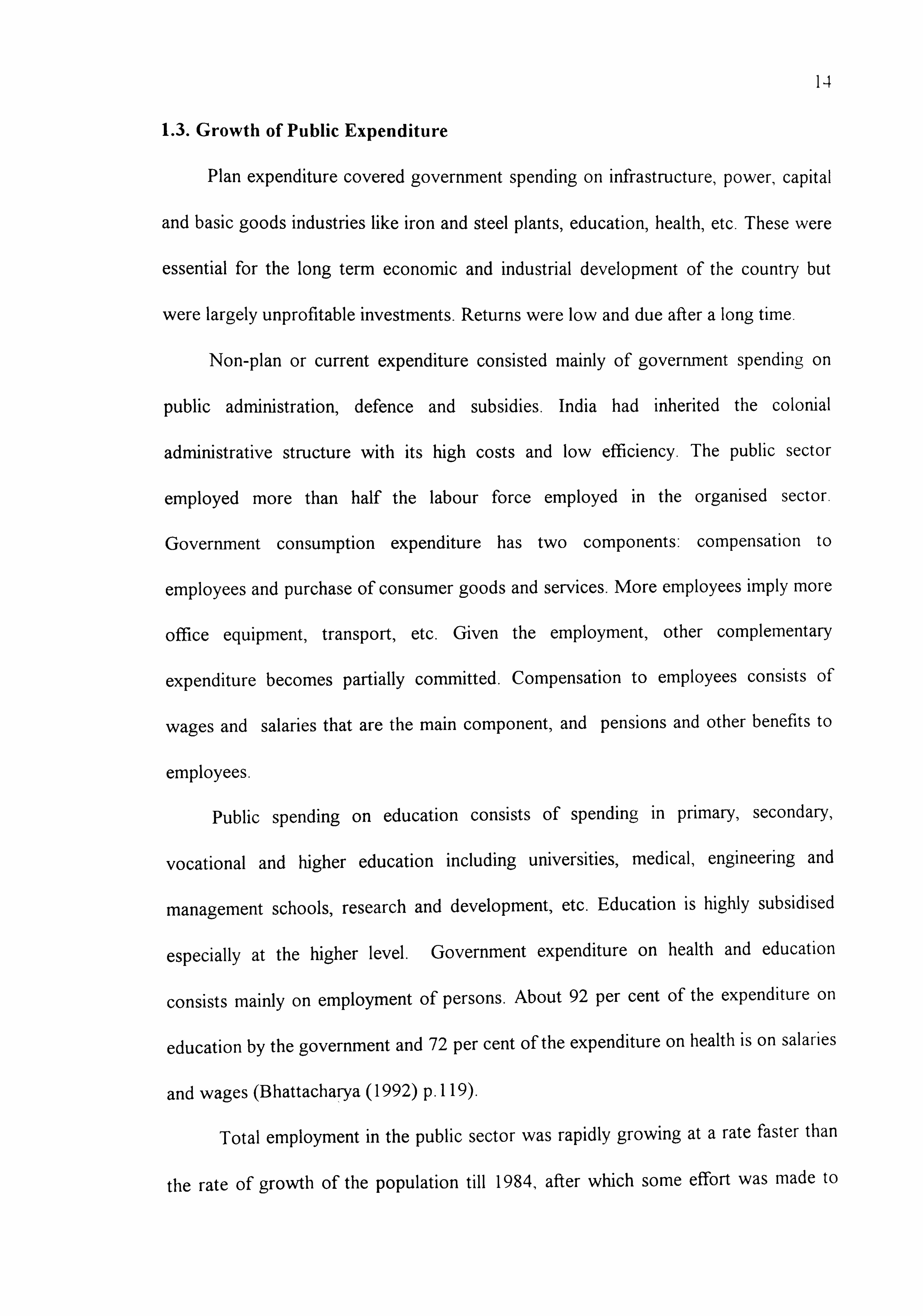
the public sector to promote the capital and basic goods industry sector. Table 1.1

shows the Gross Fixed Capital Formation in the private and public sectors as a

proportion of GDP. The relative size of the public sector remains quite high from the

second plan period right upto 1990. This can be clearly seen in Figure. 1.1.

Industrial output saw a significant deceleration in growth in the period 1966-67

to 1981-82. There is considerable debate about the cause of this slowdown in growth

rate from 6.9 per cent in the preceding decade to 5.0 during this period. Some

economists attribute it to the significant reduction in public investment that took place

at this time (Bardhan (1984)). Fixed capital formation in the public sector at 1970-71

prices grew at an annual rate of 11.3 per cent in the period 1950-51 to 1965-66, and

declined to a rate of less than half, that is 5.5 per cent, in the period 1966-67 to 198 1-

82. Since public investment accounts for nearly half the total gross fixed capital

formation in the economy and about five times the amount in the private corporate

sector, this cut back had a considerable effect on growth.

Table 1-1: Gross Fixed Capital Formation in the Public and Private Sectors as a

per cent of GDP

Year Public Sector Private Sector

1950-55 2.84 6.1

1955-60 5.26 7.54

1960-65 6.96 7.32

1965-70 6.34 8.72

1970-75 6.2 7.92

1975-80 8.02 9.88

1980-85 9.62 9.98

1985-90 10.4 11.6

1990-91 9.4 13.8

1991-92 9.5 12.7

1992-93 8.5 13.0

1993-94 8.4 12.5

Source- Economic Survey 1994-95 (1995), Government of India, New Delhi.

An important factor was also that the cut backs from the mid-sixties onwards

were on sectors like railways and electricity that were crucial for growth in the private

sector. The deceleration was seen mainly in the basic and capital goods industry where

growth rates more than halved. These included mainly heavy industries such as basic

metals, metal products, electrical and non-electrical machinery, and transport

equipment. The reduction in public investment meant a decline not only in the

infrastructure facilities like power, fuel and transport, much of which is in the public

sector, but also in the demand for the products of capital goods industries that public

investment generates.

12

14

Gross Fixed Capital Formation in the Public and Private Sectors

c

lg 12

10

8

6

4

2 (D

Public

--- ------------ Private

LO lqT r- C) CY) (D G) (N LO LO (. 0 (D (D (D r-

(3) CF)

Year

Fig. 1.1

00 T- 14t rl- C) cle) r- oo 00 00 0) CY) CY) (Y) CF) CY) (3) 0) T- T- T- Ir- Ir- T-

Agriculture was the dominant sector in the Indian economy. It accounted for

more than 50 per cent of the share of output and 70 per cent of the labour force

employed. Growth in agriculture was initially expected to take place through an

increase in irrigation and an improvement in land distribution. Food output, however,

barely kept up with the rate of growth of population. Availability of food fluctuated

greatly with rainfall. The drought in 1965 created shortages and forced India to import

large quantities of wheat from the US under PL 480. The desire to reduce external

dependence for food was crucial in bringing about the Green Revolution. Changes in

the technology of wheat production were ushered in into certain pockets of the

country which were well irrigated and where the institutional structure was conducive

to the adoption of new technology. The technology was promoted by providing a

number of subsidies on power, imported inputs, credit and machinery.

Ii

Due to the externalities and indivisibilities involved in investment in

infrastructure facilities in agriculture, public investment was crucial. Growth prospects

of Indian agriculture are vitally dependent on public investment in irrigation, drainage

and flood control, in land shaping and land consolidation, in prevention of soil erosion

and salinity, in the development of a widespread research and extension network, and

in rural electrification and provision of productive credit. The expansion of irrigation

and state and community projects for tapping groundwater through public tube-wells,

for flood control and for soil improvements can have dramatic results. Since the

average size of land holdings even among the better-off farmers is small in many parts

of the country, the capacity of the farmer to invest is limited. There is thus a need for

supplementary public investment .

1.2. Financing Development

Public expenditure in India consists of plan expenditure and non-plan

expenditure. Plan expenditure is the outlay on Five Year Plans. These include outlays

on industry, agriculture, energy, health, education, social services, etc. The main

source of financing plan expenditure was borrowing. The returns from the investments

made were expected to be adequate to pay off the debt. Non-plan expenditure was

mainly current expenditure and was to be financed by revenue. The main sources of

budgetary revenue were expected to be direct and indirect taxes and profits of public

sector enterprises. However, most public sector enterprises, except oil companies,

were running losses and had to be heavily subsidised.

14

1.3. Growth of Public Expenditure

Plan expenditure covered government spending on infrastructure, power, capital

and basic goods industries like iron and steel plants, education, health, etc. These were

essential for the long term economic and industrial development of the country but

were largely unprofitable investments. Returns were low and due after a long time.

Non-plan or current expenditure consisted mainly of government spending on

public administration, defence and subsidies. India had inherited the colonial

administrative structure with its high costs and low efficiency. The public sector

employed more than half the labour force employed in the organised sector.

Government consumption expenditure has two components- compensation to

employees and purchase of consumer goods and services. More employees imply more

office equipment, transport, etc. Given the employment, other complementary

expenditure becomes partially committed. Compensation to employees consists of

wages and salaries that are the main component, and pensions and other benefits to

employees.

Public spending on education consists of spending in primary, secondary,

vocational and higher education including universities, medical, engineering and

management schools, research and development, etc. Education is highly subsidised

especially at the higher level. Government expenditure on health and education

consists mainly on employment of persons. About 92 per cent of the expenditure on

education by the government and 72 per cent of the expenditure on health is on salaries

and wages (Bhattacharya (1992) p. 119).

Total employment in the public sector was rapidly growing at a rate faster than

the rate of growth of the population till 1984, after which some effort was made to

15

slow it down. Real wages in the public sector grew faster than per capita real national

income in the 'eighties. Average emoluments in public enterprises in 1988-89 were 9.5

times per capita real national income against 8.7 times in 1980-8 1. (Bhattacharya

(1992) p. 121-125).

Defence spending was high and rising because of external political uncertainties.

The defence budget accounts for about 4 per cent of GDP and 16 per cent of total

government expenditure. Taking related expenditure into account it is probably higher

at 5 per cent of GDP and 20 per cent of total government expenditure though it is still

relatively low in international comparison (Bhattacharya (1992)).

Subsidies on food, fertilisers and exports were rising. The share of government

expenditure on agriculture rose after the green revolution as the state provided

incentives to farmers in the form of subsidies on seeds, fertilisers, credit, etc. Real

investment, both public and private in agriculture slowed down in the 'eighties. The

sharp rise in subsidies , both open and implicit, eroded the surplus available for public

investment in agriculture to a considerable extent. (RBI (I 994), p. 109)

It is estimated that in the early seventies aggregate government expenditure was

declining in real terms. In the late seventies nominal expenditure growth rose to over

13 per cent per annum and real expenditure started growing quite rapidly. After 1979

norn-inal expenditure growth rose to 18.6 per cent but due to the higher inflation rate

real growth in expenditure remained stable. Real growth rose sharply in the period

after 1983 ( Mundle and Rao (1992), p. 230-3 1).

Another trend in the pattern of public expenditure is the declining share of capital

expenditure in total public expenditure. The economic classification of expenditure

reveals that from 1971-72 to 1987-88 the share of capital expenditure shrunk from

16

over 56 per cent of total central government expenditure to only 30 per cent. This was

mainly because of the dramatic increases in the share of interest payments, subsidies

and compensation to government employees (Mundle and Rao (1992) Table 3, p. 233)

1.4. Tax Revenue

The was a considerable growth in tax revenues over this period even though it

did not increase at the same rate as public expenditure. The tax to GDP ratio rose from

6 per cent in 1950-51 to about II per cent by 1970-71 and further to about 17 percent

in the eighties.

The increase in tax revenue was accompanied by a significant increase in the

share of indirect taxes. This was due to a fall in the contribution of direct taxes. They

fell from about 30 per cent of tax revenue in the early sixties to 14 per cent in 1989-90

(Mundle and Rao (1992) p. 236). In the 1980's there has been a slight increase in the

share of direct taxes as seen in Table 1.2.

Table 1.2: Direct and Indirect Tax revenues of the Centre and States combined

(as a per cent of GDP)

Year Direct Indirect Total

1980-81 2.6 11.9 14.5

1985-86 2.7 13.7 16.4

1990-91 2.7 13.8 16.5

1991-92 3.1 13.6 16.7

1992-93 3.2 13.0 16.2

1993-94(RE) 3.2 12.0 15ý2

Source- Reserve Bank of India Annual Report 1993-94, (1994), Bombay, Table 111.9 ,

p. 196.

17

The tax base for both direct and indirect taxes is narrow. In the case of indirect

taxes most services are completely excluded from the tax base and many goods,

especially those produced in the informal sector escape taxation. The base for personal

income tax has been rendered extremely narrow by excluding agricultural income,

administrative difficulties of taxing the unorganised non-agricultural sector and the

provision for exemptions and deductions for various purposes. The base for corporate

taxes has been eroded by making generous deductions for depreciation and

reinvestment and contributions for a wide variety of social purposes. Though

agriculture constitutes the largest sector in terms of output and employment, yet,

problems of estimation and costs of collection prevent agricultural incomes from being

taxed. This has created horizontal inequity in the system. It has prevented the taxation

of large land owners and rich farmers. It has also provided a means of tax evasion for

those who have income from both agricultural and non-agncultural sources. For the

tax payers this led to margi I nal income tax rates that were very high (up to 97 per cent).

This encouraged tax evasion. At the same time legal and tax administration machinery

was loose and tax evaders were not penalised. While the actual magnitude of income

tax evasion is difficult to estimate and different studies suggest different figures, it can

easily be said that it was large enough to considerably affect tax revenues.

Apart from the inadequate growth in tax revenues, the income from non-tax

revenues has also contributed to the growth in revenues lagging behind. Implicit

subsidies by way of unrecovered costs are provided on a whole range of social and

econormc services provided by the government.

18

1.5. Composition of Public Debt

The 1980s saw a rapid rise in public expenditure in India. The current

expenditure of the government as a ratio of GDP rose from 11.5 per cent in 1970-71

to almost 23.1 per cent in 1989-90. As mentioned above, wHe expenditure was rising,

receipts were not rising at the same rate since taxes, especially direct taxes, were not

buoyant. Over the 1980s, the gap between expenditure and receipts was increasing.

While there was a budgetary surplus in the 1970s, the 1980s saw a rise in budget

deficits. During the eighties the deficit on the budget was slowly rising and by 1989-90

the fiscal deficit rose to 12.8 per cent of the GDP. About 72 per cent of the gap was

financed by domestic borrowing, 7 per cent from external assistance and 21 per cent

from deficit financing (Economic Survey, 1990-9 1).

Till the rrud-1980's, the government bond market was more or less a captive

market as government securities were bought by financial institutions like banks and

insurance companies to fulfil their Statutory Liquidity Ratio (SLR) requirements,

which had risen to 38.5 per cent, even though rates of interest on government bonds

were very low and even negative in real terms. If public debt was larger than the

amount the financial institutions had to hold, then the surplus would be monetised as

the Reserve Bank of India was obliged to lend to the government. In the 1980s special

government bonds were issued under various schemes like the Indira V1kas Patras and

Kisan Vikas Patras at non-iinal rates of interest of up to 9 to 10 percent. In addition, tax

concessions were given to those who purchased these bonds. The high interest rates of

government conu-nercial borrowing from households as well as the tax concessions

proved to be a burden on the exchequer.

19

This led to a substantial increase in interest payments made on public debt. The

rising interest payments since the 1980's are a consequence of three factors -the

increase in total debt, the increase in the interest rate and the increase in the

proportion of high interest bearing liabilities in the government's debt. The internal

liabilities of the Government of India have been classified into two categories, the

"internal debt " and the "other liabilities". The internal debt consists of (i)market loans,

(ii) Treasury Bills, (111) Special Securities issued to the RBI, (iv) Special Bearer Bonds,

and (v) Balances of expired loans, Prize Bonds, Premium Prize Bonds, etc.. "Other

liabilities" comprise (i) small savings, (ii) state provident funds, (111) Public provident

fund etc. These so-called "other liabilities" carry a higher rate of interest than internal

debt and there has been a rise in the proportion of "other liabilities" in the government's

total liabilities. The consequence of higher interest payments is a significant rise in the

magnitude of public debt. Table 1.3 shows the sharp increase in the debt/GDP ratio

since 1980-81.

Table 1.3: Total Outstanding Liabilities of the Government of India (as a per

cent of GDP)

Year Total Liabilities

1980-81 43.9

1984-85 49.0

1985-86 52.4

1990-91 59.1

1991-92 57.8

1992-93 57.0

1993-94(RE) 58.7

Source- Reserve Bank of India, Annual Report 1993-94, (1994), Bombay, Table 111.4 ,

19 1.

110

This led to widespread concern at the rising public debt and a number of studies

like Seshan (1987), Rangarajan el aL (1989), Buiter and Patel (1990) and Chelliah

(1992) concluded that the path was unsustainable. However, no serious attempt was

made to curtail government borrowing. This was despite an official declaration of

intent to arrest further deterioration of budget deficits made in the Long Term Fiscal

Policy (LTFP) statement of 1985 which suggested certain specific measures to reverse

the decline in public savings -a reduction in subsidies and unproductive adnunistrative

expenditure and increasing the contribution of public enterprises through proper

pricing and other policies. The Centre's borrowing remained at 7 per cent of GDP

against the target of 4 per cent set by the LTFP and public saving did not go beyond

2.4 per cent despite the target of 4 per cent. The seventh five year plan finalised in

1985 provided for a rate of growth of non-plan expenditure no higher than the rate of

growth of GDP in an attempt to contain public borrowing. But the growth of non-plan

expenditure was three times as high during the seventh plan period (Jalan (1992)).

1.6. The External Crisis

At the same time , during the 1980s, a balance of payment crisis was developing.

1979 saw the second oil price shock and a rise in US interest rates and LIBOR raising

the burden of servicing the existing external debt. Due to the recession in industrial

countries and the uncompetitiveness of the exchange rate, export growth was slow.

Some attempts at liberalisation saw growth in new industries like automobiles

and electronics, both heavily dependent on imports of technology and components. As

the economy grew at relatively much higher rates of growth of 5.5 per cent over the

21

decade, imports grew rapidly. The widening current account deficit was Increasingly

financed by non-concessional loans. According to World Bank debt data, India's total

outstanding foreign debt increased from $18.7 billion in 1980 to $56.3 billion in 1989

and debt to private creditors increased from about $2 to $21.4 billion during this

period ( Jalan(1992)). The Gulf crisis resulted in a higher import bill and a loss in

foreign remittances. The collapse of the USSR and Eastern Europe led to a decline in

Indian exports.

The above trends led to a balance of payment crisis in June 1991. India was left

with only two weeks imports worth of foreign exchange. Her credit rating fell sharply

and foreign private lending was cut off For the first time there was a serious possibility

of default. Faced with this crisis the government was forced to act.

1.7. Stabilisation and Structural Adjustment

Emergency stabilisation measures aimed at reducing inflation, which had risen to

12 per cent, and the current account deficit, that stood at 3 per cent of GDP and 40

per cent of exports, were taken. Emergency import controls, that were later eased,

were imposed. Gold backed external borrowing was undertaken. The rupee was

devalued by 22 per cent. A scheme of tradable import entitlements for exporters was

introduced. A tight monetary policy implied reducing money supply and raising rates of

interest. The July 1991 budget set a target for reducing the central government's fiscal

deficit from 9 per cent to 6.5 per cent of GDP.

The immediate aims of the measures were to bring the current account deficit to

2.7 per cent of the GDP and inflation down to 9 per cent. Loans were negotiated with

the IMF and the World Bank for stabilisation and structural adjustment. The reforms,

1) 1)

as outlined in the letters of intent from the finance minister to the IW and the World

Bank, were designed to remove impediments to domestic and foreign private

investment and to deregulate industry. The import regime was drastically simplified ,

tariffs were reduced, export subsidies simplified and the rupee made convertible thus

letting market forces determine the exchange rate. This trade and exchange rate

liberalisation was also accomparned by tax reform, reform of public sector enterprises

and the financial sector which had direct implications for the fiscal deficit. The tax

reform consists of a cut in import duties, a streamlining of personal taxes- a cut in tax

rates and a reduction in exemptions, restructuring of capital gains and wealth taxes.

New measures include an increase in the corporate tax rate, a reduction in generous

depreciation allowances that had tended to encourage capital- intensive methods of

production, a tax on the gross interest receipt of banks, increases in excise duties, and

a reduction in the rates of import duties. 2

The reform of the financial sector consists primarily of a reduction in the

Statutory Liquidity Ratio and a rationalisation of subsidised credit to priority sectors,

relaxation of interest controls and restrictions on firms' access to capital markets, and

more autonomy to public sector banks. The major reform in the case of public sector

enterprises consisted of eliminating privileges such as protection from external and

domestic competition and preferential access to budget and bank resources. Though

the condition relating to an effective 'exit policy' for closure or restructuring of money

loosing firms in the private and public sector has not been fulfilled, the reforms made

have largely been in line with the programme's objectives.

2- Memorandum of Economic Policies for 1991-92 and 1992-93', in U. Kapila, (ed), 'Recent Developments in the Indian Economy'

Part-1, p. 322

23

The most important change appears to be in the opening up of the economy to

foreign capital and the removal of exchange restrictions on imports. Consequently, in

1994 India attained Article VIII status and joined the ranks of the 96 other such

member countries of the M. International monetary arrangements after the Bretton

Woods Conference required members of the EMF to restore current account

convertibility. The obligation as defined in Article VIII ,

Sections 2,3 and 4 stipulates

that member countries should have no restrictions on current payments and avoid

discriminatory currency practices. The first major step towards current account

convertibility was taken with the unification of the exchange rate and the removal of

exchange restrictions on imports through the abolition of foreign exchange budgeting

at the beginning of 1993-94. Relaxation in payment restriction in the case of a number

of invisible transactions followed the budget for 1994-95. In August 1994, the final

step towards current account convertibility was taken by further liberalisation of

invisibles payments and acceptance of the obligations VIII of the RVIU, under which

India is conunitted to forsake the use of exchange restrictions in current international

transactions as an instrument in managing the balance of payments.

In 1993-94 imports stood at 10.5 percent of GDP. External debt had been

reduced from 41 percent in 1991-92 to 40 per cent in 1992-93 and further to 36 per

cent in 1993-94. Direct foreign investment quadrupled from $150 million in 1991-92 to

$620 million in 1993-94. In the first half of 1994-95, it was 50 per cent higher than in

the first half of 1993-94 (Economic Survey 1994-95, p. 9). The current account deficit

was brought down to nearly 0.1 per cent of GDP in 1994-95. While the reforms appear

to be successful in the context of the external sector, their success as far as the

government expenditure and deficit is concerned appears to be limited.

24

1.8. Cut in Development Expenditure

The rates targeted for the reduction in fiscal deficit have not been achieved. For

example, though the gross fiscal deficit (GFD) was brought down from 8.39 per cent

of GDP in 1990-91 to below 6 per cent in the next two years, there was a deterioration

in the following years. The GFD to GDP ratio increased to 7.3 per cent in 1993-94

(Revised Estimates) as against budget estimates of 4.7 per cent. As data from the RBI

Annual Report 1993-94 indicates there was an increase in the revenue account gap

from the budget estimates of 2.3 per cent of GDP to 4.2 per cent of GDP. This may be

explained by both the shortfall in revenue proceeds and the overruns in expenditure.

The shortfall in revenue receipts in 1993-94 accounted for 37.2 per cent of the total

increase in GFD during 1993-94. This was due to the decline in customs and excise

duties due to sluggish industrial activity and the reduction in custom duty rates. Total

revenue collection was 9.6 per cent lower than estimated in the budget. In the

following years, including in the 1995-96 budget, there has been a further reduction in

custom duties which would reduce revenue collection from this source. Expenditures

also grew by 9.6 per cent over the budget estimates; subsidies were 48.0 per cent

higher while defence was 12.1 per cent higher. Both food and fertillser subsidies

increased. Since 1992 the government has taken some steps in an attempt to cut the

growth of consumption expenditure. These include a reduction of posts at various

levels, overall cut in consumption of petrol, diesel, reduction in expenditure on

telephones and restriction on purchases of additional vehicles. The strength of the staff

of the Central Government showed an estimated decline of about fifty thousand from

March 1992 to March 1994 (Economic Survey 1994-95, p. 16). However,

25

consumption expenditure still grew from 3.8 per cent of GDP to 4.1 per cent of GDP

from 1992-93 to 1993-94 and led to a rise in revenue deficit.

Another major area of concern is the growing interest burden that accounted for

43.8 per cent of total non-plan expenditure and 53.4 per cent of revenue receipts in the

1994-95 budget. As discussed earlier this is the consequence of the high fiscal deficits

in the eighties that have resulted in the accumulation of a large public debt and of the

application of market related interest rates in the sale of government securities that has

led to an increase in the service cost on internal debt.

Table 1.4: Measures of Dericit of the Central Government (as a per cent of GDP

at current market prices)

Year Gross Fiscal Net Primary Revenue

Deficit Deficit Deficit

1980-85 6.26 2.99 1.11

1985-90 8.21 3.80 2.58

1990-91 8.39 3.32 3.49

1991-92 5.90 1.46 2.64

1992-93 5.69 1.66 2.63

1993-94 4.71 0.44 2.25

(Budget Estimate)

1993-94 7.29 2.72 4.24

(Revised Estimate)

Source: Reserve Bank of India, Annual Report 1993-94, (1994), Bombay, Table 3.1 ,

3 5.

In recent years there has been an increase in net primary deficit (defined as GFD

less net lending less net interest payments). As Table 1.4 shows it has increased from

1.7 per cent of GDP in 1992-93 to 2.7 per cent of GDP in 1993-94 despite the target

'-)

of 0.44 per cent. This is likely to lead to a further rise in the debt to GDP ratio and

interest burden in the future. Total debt servicing consisting of interest payments and

repayment of debt was 112.8 per cent of total revenue receipts in 1993-94 (Economic

Survey 1994-95). Table 1.4 also shows that instead of falling from 5.7 per cent to 4.7

per cent from 1992-93 to 1993-94 as was the budget estimate, the Gross Fiscal Deficit

rose to 7.3 per cent.

The sharp deterioration in the revenue deficit has changed the composition of the

G. FD such that it explained 58 per cent of GFD in 1993-94 as against 46 per cent in

1992-93 and 17.0 per cent in the first half of the eighties. In other words, 58 per cent

of government borrowing in 1993-94 was to cover current expenditure. There was a

squeeze in capital outlay from 2.3 percent of GDP in 1990-91 to 1.6 per cent In 1993-

94 ( RBI (1994), p. 36-37)

The State Government budgets also show a similar trend "large budgetary gaps

particularly on revenue account, rising non-developmental expenditure, reduction in

the availability of resources fo r investment and a sluggish revenue

performance. "(RBI, (I 994) p. 42) The overall deficit nearly doubled from 1993-94 to

1994-95 while revenue deficit went up by one-third. The GFD is thus expected to be

28 per cent higher. As compared with an average surplus of 16.8 per cent of GFD in

early eighties, the revenue deficit was 28 per cent of GFD- Consequently, as compared

to only 7.7 per cent of overall borrowing being utilised to finance current expenditure

in the latter half of the 'eighties, 28.1 per cent of the overall borrowing was siphoned

off to finance current expenditure. The availability of funds for capital outlay and net

lending that reflects the states' investment operations gets correspondingly reduced.

While the central government had greater flexibility in its budget as it could borrow

I

from the public, the access of state governments to public borrowing was much more

limited. Consequently, state government's showed substantial shortfalls in actual

outlays in relation to plan projections. Since the primary responsibility for investment

in social sectors, agriculture and irrigation is that of the states, there was a dech in ne

these areas (Jalan, 1992).

The composition of expenditure shows that non -development expenditure (i. e.

interest payments, administrative services, pensions and miscellaneous general

services) rose faster than the development component from an average of 22.9 per cent

in the late eighties to 3 1.1 per cent in 1994-95.

The increased reliance on borrowing both from the Centre and the market

implies higher repayments and interest payments in the future which would further

curtail development expenditure. For the Centre and State budgets combined the rising

committed outlays for interest payments and administrative expenses have increased

from 9.9 per cent of GDP in 1985-86 to 11.6 per cent in 1993-94. The combined

government sector capital outlay has declined from 5.0 per cent to 3.2 per cent of GDP

over this period. The share of non-development expenditure has increased from 32.4

per cent to 42.4 per cent of total expenditure over this period and is expected to rise

further.

The overall picture that emerges from the above account of government

spending and expenditure is a fall in the proportion of capital outlays and development

expenditure in total government expenditure. Table 1.5 shows that the proportion of

development expenditure has declined by more than 10 per cent since 1980.

28

Table 1.5: Development expenditure of Centre and States (as a per cent of total

expenditure)

Year Development Expenditure

1980-81 66.0

1984-85 64.6

1985-86 65.1

1990-91 58.8

1991-92 55.5

1992-93 55.7

1993-94 (R. E) 54.3

Source-. Reserve Bank of India Annual Report 1993-94, (1994), Bombay,

Table 111.10 , p. 197.

To analyse the effect of the ongoing changes in government expenditure and debt

in India we shall first test the Ricardian equivalence hypothesis. We then present a

general model encompassing both the Ricardian and the non- Ricardian models. This

model is estimated for India to determine the underlying behavioural parameters that

are crucial in determining the impact of debt on growth. Finally, we present a model of

endogenous growth driven by capital externalities arising from both private capital and

public capital and infrastructure. Since the fiscal deficit is equal to the revenue and

capital expenditures and net domestic lending minus revenue receipts and grants

measuring the overall resource gap, it is possible to reduce it by a cut in capital

expenditures rather than government consumption expenditure. Therefore, we examine

the effect of not just government borrowing, change in tax rate and the change in the

ratio of public investment to total government on long-run growth rate of the GDP.

We limit the scope of this study to the effects, rather than the causes for the

growth in non-development versus development expenditure. The political economy of

29

the forces that generate the pressures on current expenditures of the government at the

expense of public investment in India is another study in itself (for example, Bardhan

(1989)).

30

Chapter 2

Debt Neutrality

Theory and Evidence

Standard econonk theory suggests that an expansionary fiscal policy raises

aggregate demand in an economy. It leads to a reduction in private spending, especially in

private investment associated with an increase in real interest rates caused by fiscal

expansion. This phenomenon is referred to as 'crowding-out'. Barro, (1974) suggested that

the underlying premises of the crowding out hypothesis is that consumers perceive a cut in

taxes to be a rise in permanent income. If consumers were rational and far sighted, they

would expect a cut in current taxes to be followed by a rise in taxes at some time in the

future. They would, therefore, not perceive the cut as a rise in permanent income and

would not change their consumption levels. This hypothesis has come to be known as

Ricardian EquiValence. '

In this chapter we shall discuss the Ricardian Equivalence theorem of debt-

neutrahty. Section I sets out the representative agent model. Section 2 introduces the

govenunent into the model and discusses Barro's hypothesis. Section 3 examines some of

the evidence on Ricardian Equivalence. In section 4 we exarnine the evidence for India.

2.1 A Representative Agent Model

Consumption is determined by fife-tune resources rather than income in the current

period. Life-time resources represent permanent income which can be thought of as a

constant resource flow that can be sustained throughout the planning horizon. If current

income exceeds permanent income, the individual saves. He can acquire physical or

' The hypothesis is associated with Ricardo( 1951) in whose vntings this idea finds its first articulation. Even though Ricardo had doubts about the equivalence hypothesis, the proposition continued to be linked with his name. '17he terin Ricardian Equivalence %vas first introduced to macroeconomists by James Buchanan ( 19 76).

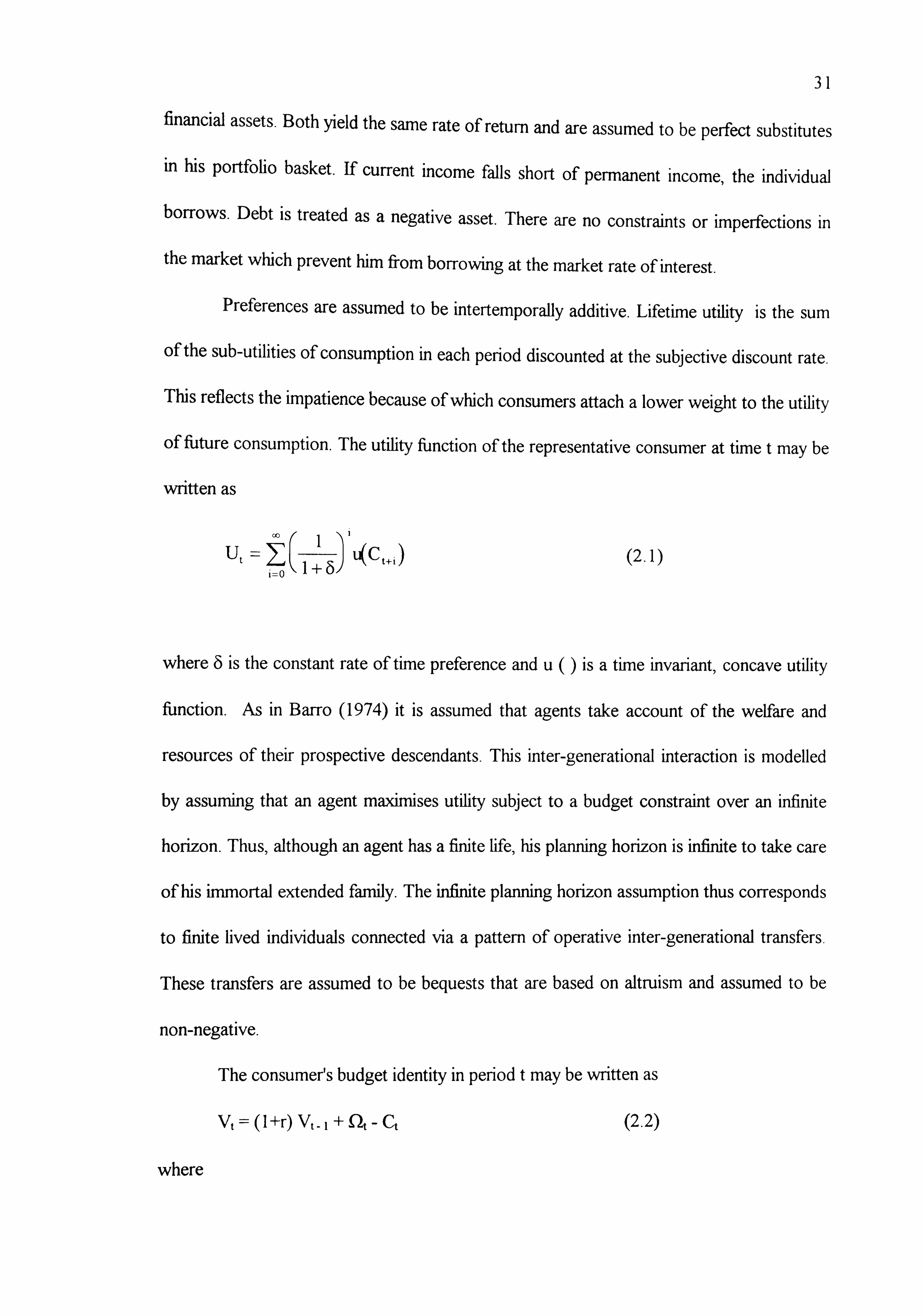
31

financial assets. Both yield the same rate of return and are assumed to be perfect substitutes in his portfolio basket. If current income f9s short of permanent income, the individual borrows. Debt is treated as a negative asset. There are no constraints or imperfections in

the market which prevent him fi7om borrowing at the market rate of interest.

Preferences are assumed to be intertemporafly additive. Lifetime utility is the sum

of the sub-utilities of consumption in each period discounted at the subjective discount rate.

This reflects the impatience because of which consumers attach a lower weight to the utility

of future consumption. The utility function of the representative consumer at time t may be

written as

ut

= (-ýZ, ), 4c 1 t+i i=O

(2.1)

where 6 is the constant rate of time preference and u() is a time invanant, concave utility

function. As in Barro, (1974) it is assumed that agents take account of the welfare and

resources of their prospective descendants. This inter-generational interaction is modelled

by assurning that an agent maximises utility subject to a budget constraint over an infinite

horizon. Thus, although an agent has a finite fife, his planning horizon is infinite to take care

of his immortal extended family. The infinite planning horizon assumption thus corresponds

to finite lived individuals connected via a pattern of operative inter-generational transfers.

These transfers are assumed to be bequests that are based on altruism and assumed to be

non-negative.

The consumer's budget identity in period t may be written as

(I+r) V, I+ f4 - C, (2.2)

where

12

Vt = non-human wealth at the end of pefiod t

r= rate of interest assumed constant

Q= consumption in penod t

f2t = post tax labour income in pefiod t

Rearranging (2.2) and solving forward in time the budget identity become the solvency

constraint

00

+ r)v, -, [ct+i

- Qt+i (2.3)

provided that the transversality condition lim Vt+i :::::: 0 i-400

-(I + r)

does not grow at a rate faster than the rate of interest.

holds or that wealth

The representative agent's intertemporal budget constraint implies that the total

value of consumption over time is equal to the total human and non-human wealth

possessed by the consumer. Non-human wealth is represented by V, and includes the

financial and non-financial assets owned by the consumer. Human wealth is the present

value of a future stream of disposable income and may be represented by

i=o + r) t+i (2.4)

Maximising the representative individual's objective function (2.1) subject to the

intertemporal budget constraint (2.3), we obtain the first order condition

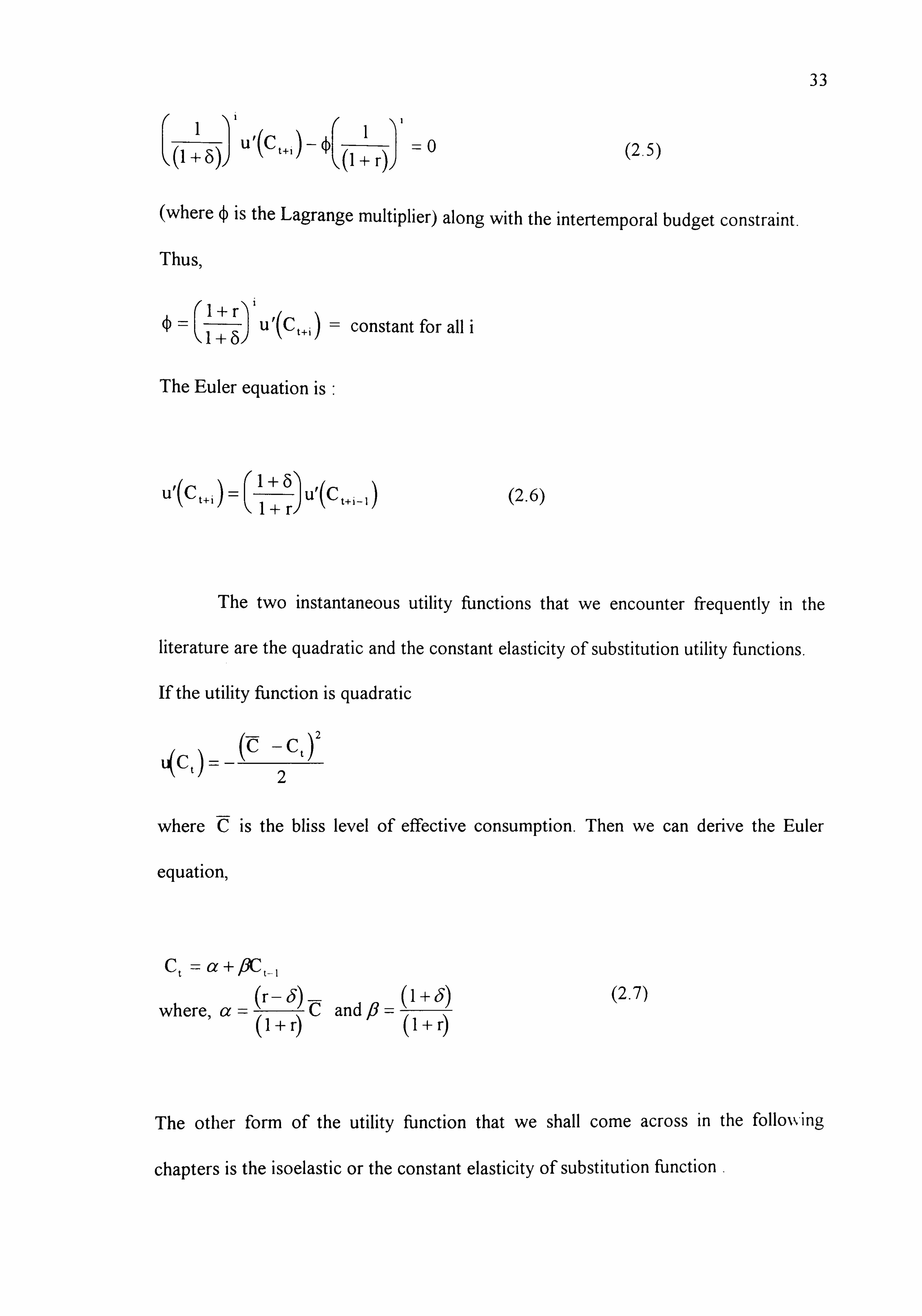
33

++ r) (2.5)

(where ý is the Lagrange multiplier) along with the intertemporal budget constraint.

Thus,

constant for all i

The Euler equation is :

u'(cý) =1+ öu(c+11) 1+ r)

(2.6)

The two instantaneous utility functions that we encounter frequently in the

literature are the quadratic and the constant elasticity of substitution utility functions.

if the utility function is quadratic

Ct) 2

Ct

where C is the bliss level of effective consumption. Then we can derive the Euler

equation,

Ct -a+, 8Ct-,

where, a 9)

+ r) and, 8 =

(I (I +0

(2.7)

The other form of the utility function that we shall come across in the following

chapters is the isoelastic or the constant elasticity of substitution function .

34

U(c ct CY

ln(Ct)

if YCF > 0, YCY

if G=1

(2.8)

where cy is the intertemporal elasticity of substitution. It measures how responsive is

the ratio of consumption in the two periods to relative prices. Estimates of cy vary

substantially but usually lie around or below unIty ( Blanchard and Fischer(1987)

p. 44). In case cy = 1, the utility function is logarithmic in form. In the case of the

logarithmic utility function the Euler equation is linear and of the form

C= al- t P'-t-i

where, P r) (1+45)

(2.9)

2.2. The Ricardian Equivalence Hypothesis

If it is assumed that the utility function is logarithmic then by combining (2.9)VVqth

the budget constraint (2.3) we can show that

ct = ýt IWO Vt-l + Yý (2.10)

where ýt = 6/1+6. and it represents the marginal propensity to consume out of lifetime

wealth which consists of human and non-human wealth. (2.10) represents the consumption

function of the representative agent. Since R is the discounted value of post tax labour

income, it is not independent of taxes.

We now introduce the government into the model. It can be shown that policies that

have a transitory effect on income are incapable of having an effect on consumption.

35

We can then demonstrate that if it is assumed as in Barro(1974) that consumers

understand the implications of the government budget constraint, they do not regard a

tax cut , given government spending , as permanent. They are fully aware that a cut in

contemporaneous taxes implies a future tax increase. Hence, under these circumstances

a tax cut leads to no change in consumption. It leads to only a transitory change in

income which has no effect on consumption.

It is assumed that the government obtains no revenue from the creation of money.

The government sector has a budget identity of the forrn

Dt = (I + r)Dt -1+ Gt - Tt

where D, is public debt at the end of period t.

D- Rearranging and solving forward in time, the budget identity (2.11) becomes the solvency

constraint

-

co I-G (2.12) +r) D,

- [Tt+i

t+i iýo -(I+

r)-

provided that the transversality condition lim D=0 holds. According to t+1 J, + r)

a government vAth a positive debt must eventually run primairy surpluses to be

solvent. This is a weak solvency condition as the government can be solvent even though

its real debt and its debt/GDP ratio grows WIthout a bound. Our definition of solvency

merely requires that this ratio does not grow faster than the growth adjusted real interest

rate in the long run. It does not require a stable debt/GDP ratio which is referred to as a

strong solvency condition (Buiter and Patel(I 99 1), Krichel and Levine (1995)).

The Ricardian equivalence theorem assumes that the representative individual is

"forward looking" and rational in regard to the fiscal affairs of the government. He

'36

understands the implications of the intertemporal government budget constraint

specified in equation (2.12). He recognises the future tax obligations implicit in the

issue of current period and existing government debt and its servicing. We can rewrite

the individual's intertemporal budget constraint as

00 co ct+l + r)vt-, + [Nt+i - T+i

i=o -(I + r)- j=0 + r)

since Q, = N, - T,

where N, = labour earnings in period t (assumed to be exogenous) and

T, = Tax payments (net of transfers) in period t.

We can integrate the private and public sectors by substituting the government

constraint into the representative agent's budget constraint. The budget constraint of

the representative individual is now

co c

i=o + r)

t+l = (I + r)[V, -, - D, -,

] co I

(N, +i

G, +I)

1=0 +

(2.13)

Thus if the agent is rational and understands the government's budget constraint and

incorporates it into his own, his intertemporal budget constraint is represented by (2.13).

Using (2.10) we can now show that

00

c -D ]+I] (Nt+i - Gt+j) (2.14) i=o

(I + r) t (I + r)lvt- t-I

The consumption function of the rational representative agent is now independent

of the level of taxes or debt issued in period t or after. Any change in taxes leaves

37

consumption unaffected. A fise in govemment spending has a negative net wealth effect

and reduces consumption. This is because the government would have to raise taxes at

some time to pay for higher spending, thus reducing the lifetime wealth of the consumer.

(2.14) therefore represents the consumption function corresponding to the Barro-Ricardian

model. Keeping the level of government spending constant , it demonstrates that if the

consumer incorporates the government's intertemporal budget constraint into his own, a

change in the level of taxes does not affect his life-time wealth i. e. it has no net wealth

effect. A shift fi7om current taxes to a deficit has no impact on aggregate demand.

2.3. Empirical Studies

The most common approach to empiricaHy test the Ricardian theorem was to

include fiscal variables in a regression of private consumption in order to test whether a

debt financed tax cut led to an increase in private consumption expenditure

(Feldstein(1982), Kon-nendi(1983)). Pfivate consumption was specified as a ffinction of

income, taxes., government expenditure and private wealth including public debt and the

proposition was tested in terms of the restrictions placed on these. The model was

estimated usuatly for the US. Differences in measurement and restrictions led to different

conclusions. This approach was criticised on the grounds of the arbitrariness with which

variables were included or excluded from the model. Tl-ýs resulted from not specifying the

underlying theoretical model. The approach did not explicitly test the assumptions of the

equivalence proposition and expectations behaviour was not incorporated into the

estimating model. FoHowing Aschauer (1985) we defive a model based explicitly on

Ricardian assumptions and a government expenditure expectation function based on

rational expectations.

38

We assume that utility is a function of the total consumption by an individual of

both public and private goods.

C* =C +OG tt (2.15)

where C* denotes the level of "effective" consumption in period t. It Is a linear t

combination of private consumption Ct . and government goods and services G,. In

terms of effective consumption, the budget constraint of the representative individual

is:

00 00

ct+1 :: -- (1+ r)[V, -, - Dt-, ]+1 (Nt, + (0 - 1) G, + r)- i=o -(I

+ r)-

Thus the present discounted value of effective consumption is constrained by

the economy wide wealth plus the present discounted value of labour earrungs plus

(0- 1) times the value of government expenditure. Rearranging

(I + r)D, (I + r)V, Go

-N -(O-I)G, +i]=0(2.16) t+i t+i i=O 1+ r)

Maximising effective consumption (2.15) subject to the budget constraint (2.16) and if

the utility function is assumed to be quadratic then

ct

= cc +

where, a (r - and

(2.17)

+ r) + r)

39

where C is the bliss level of effective consumption. If E, is the expectations operator

conditional on information available up to period t then the expected consumption in

period t may be defined as

E C*=oc+ PC* +pt tt t-I

where p, is the error term.

Lagging equation (2.15) by one period and substituting into equation (2.18) gives

EtC*t = u. + P[Ct-I + OGt-l ]+ pt - Ct + OGt + Ct (2.19)

where EC*=c* ttt

If G, = E, -,

G, + X, (2.20)

where Xt is the error term.

We obtain

cc + PC, -,

+ POG, _1 --

Ct+ OEt-I Gt +ýt

Or, Ct =a+ PCt_l + POGt-l - 0E, _1

Gt + ýt

(2.21)

where the error term ýt includes the effect of measurement errors, revisions in

expectations and shocks.

The value of government spending is predicted on the basis of past values of

govemment spending and deficits. It is assumed that E, _1

G, the expected value of G, at

time t- I is given by

Et- I Gt =y+ 6(L)Gt- I+ co (L)FDt- I+ vt (2.22)

40

where L is the lag operator and FDt is the government deficit in period t. The error

term vt is such that it satisfies the orthogonality condition E(vtj 1, -, )=0,1, being the

information set available to the agent at time t so that vt is serially uncorrelated. If

expectations depend only on last period's spending and deficits he obtains the

following the two equation system

Gt =y+F, Gt-I +w FDt-j + vt (2.23)

and

Ct = cc' + PCt-I + fl G, + ODt-I + 7r,

where cc' = cc - Oy Tj = O(p

- F- ) (2.24)

ýt -- (1)

Ricardian Equivalence requires that the cross equation restrictions are not

violated because they imply that the consumer takes the government's tax and

expenditure decisions into account. As expectations are assumed to be rational the

government's behaviour which satisfies the intertemporal budget constraint is correctly

predicted by individual consumers.

Aschauer(1985) found evidence in support of Ricardian Equivalence. He

reports that the estimated coefficient on the lagged value of consumption is highly

significant and equal to unity implying that holding fixed the level of government

spending - private consumption expenditure follows a random walk. The point estimate

for substitutability of public spending for private consumption is positive and is

significantly different from zero at the five percent level.

41

Further, likelihood ratio statistics suggest that the data does not reject the

hypothesis at conventional significance levels. First government spending and

consumption functions are estimated subject to the restrictions on consumption. Next

the system is estimated without imposing the restrictions. To test the hypothesis of

Ricardian equivalence he examines the validity of the restrictions. This is done by

calculating the log-likelihood ratio test statistic. If Ll is the value of the likelihood

function for the maximum of the unconstrained model and LO is the value when the

constraints are imposed then the likelihood ratio test statistic is computed as LR

2(LI-LO). This statistic has a X2 distribution with degrees of freedom equal to the

2 number of restrictions. If the estimated value of LR is less than the value of the x

distribution at a given level of significance then it indicates that there is no significant

discrepancy between the constrained and the unconstrained values of the log-likelihood

function and thus we the null hypothesis that the constrained model is- true cannot be

rej ected.

Gupta (1992a) estimates the model for some developing countries. IFEs results

are mixed. IFEs evidence suggests that the coefficient of lagged consumption is

statistically significant and positive in all cases and is not significantly different from

unity in most cases. In India it is 0.65 and is significantly different from unity. 0 the

coefficient of government expenditure in India is negative and is found to be

statistically different from unity. However, the null hypothesis of Ricardian

Equivalence cannot be rejected by the likelihood ratio test.

42

2.4. Excess Sensitivity

The Ricardian Equivalence hypothesis assumes the existence of perfect credit

markets. Evidence indicates a role for current income in explaining consumption over

and above that which is due to a revision in expectation of future income as signalled

by current income (Flavin(1981), Hayashi(1982), Jappelli and Pagano(1989)). Flavin

(198 1) analysed the role of current income in providing new information about the fUture.

She found that the response of consumption to current income was beyond that attributable

to the role of current income in signal-ling changes in permanent income. The permanent

income hypothesis suggests that individual consumption depends on the resources

available to the consumer over his entire lifetime. However, if a consumer is

constrained by credit market imperfections and is unable to borrow and lend the

amount he requires to undertake his optimal consumption plan then his desired

consumption will be constrained by his current income.

To take account of the 'excess sensitivity' of consumption to current income,

Hayashi (1982) explicitly included the presence of some households in the economy who

consume only their current income. The 'excess sensitivity' of consumption expenditure

to contemporaneous disposable income may be attributed to liquidity constraints. If

liquidity constrained consumers are significant in proportion then aggregate consumption

reveals excess sensitivity to current income.

The economy is assumed to comprise of two groups of consumers - the liquidity

constrained consumers and the unconstrained consumers.

43

Aggregate consumption is assumed to be the sum of the consumption of

constrained and unconstrained consumers.

Ct = Cý + ctu

where

Q= Aggregate consumption

Ct C= Consumption of constrained consumers

Cý = Consumption of unconstrained consumers

(2.25)

We assume that unconstrained consumers receive a proportion k, of total post

tax labour income, f4. Constrained consumers thus receive a proportion (I - ?, ý ) of total

post tax labour income. Since they consume their current income,

ct c= (I -x )f4 (2.26)

If the value of ý. is estimated to be unity, then one can conclude that all consumers are

forward looking. The aggregate consumption ffinction is thus a generalisation which

includes the permanent income hypothesis as a special case.

The consumption of unconstrained consumers may be defined following (2.7) as

cu -oc+PCu , +e, t t- (2.27)

where the error term e, is assumed to be normally distributed and uncorrelated to any

information available to the consumer in period t- I including consumption in period

t-1. Since changes in current income signal changes in future income, the error term

44

may include changes in consumption expenditure which occur due to the revision in

expectation of future income.

Aggregate consumption may be defined using (2.25) and (2-27) as Cý

Ct =a+ ocu +Cc +e t- tt (2.28)

Adding and subtracting OCt-I on the right hand side we get

ct + o(CU + cc cc +e t-I t-, )+Ct -oct-I t (2.29)

Lagging (2.26) by one time period and substituting in (2.29) and using (2.25) we

obtain

ct =a+ oct- I+ (I - k)(Qt - ont-, )+ et (2.30)

X can be interpreted as the degree of excess sensitivity of consumption to current

income. If there exist no credit constraints k should be one.

2.5. Evidence for India

To test the hypothesis for India we estimate (2.27), the constrained

model, and (2.30), the unconstrained model. The model is estimated using annual data

for India for the penod 1960 to 1989. The data source is International Financial

Statistics published by the IMF (various issues). Variables are measured in real per

capita terms. Per capita GDP is used as an instrument for f2t, the current disposable

income. Since the error term may be correlated with f2t, we estimate the model by

using instrumental variables. NLIV estimates using one period lagged values of

consumption, income, private sector investment and government spending are

presented in Table 2.1. We compute the Wald statistic to test the restrIction.

45

Table 2.1 : Excess Senstivity of Consumption

Parameter Estimate [p values in parentheses]

a 15.09 [0.039]

p 0.30 [0.111]

I-k 0.547 [0.000]

Durbin Watson Statistic 1.93

LM test for first order

Serial Correlation 0.12 [0.727]

LM test for functional form 1.64 [0.201]

LM test for Heteroscedasticity 2.39 [0.122]

LM test for Normality 2.80 [0.247]

Wald test of restriction (k = 1) = 142.3 5

Wald Statistic indicates that the restricted model is not the true model.

This indicates that there is evidence of excess sensitivity of consumption to income.

This suggests that the assumption of the Ricardian model that there are perfect credit

markets is not true for India. The estimate of excess sensitivity may however be biased

because we have not taken into account the effect of other possible violations of the

Ricardian model into account. For instance, the presence of finite horizons, rather than

infinite horizons as assumed here, would lead to a greater response of permanent

income unconstrained consumers to current income than suggested by the model

46

n I, above. The would mean that our estimate of the degree of excess sensitivity, (1-ý, ) the

proportion of income received by constrained consumers, is higher than what it would

be if we took into account finite horizons. In the next chapter we extend the model to

include the assumptions of finite horizons and population growth.

47

Chapter 3

The Aggregate Consumption Function: Finite Horizons, Liquidity Constraints and

Population Growth with Income Redistribution

The model presented here is confined to the analysis of a closed economy. Non-

Ricardian effects are introduced in the aggregate consumption function by the inclusion of

liquidity constraints following Hayashi (1982), finite horizons following Blanchard (1985),

population growth following Weil (1989) and aflowmg for a transfer of consumers fi7om the

group of constrained (unconstrained) to the group of unconstrained (constrained)

consumers. Any one of these factors leads to a deviation from Ricardian Equivalence. Time

is discrete following Frenkel and Razin (1992).

3.1. Liquidity Constraints

As described in Section 2.5 the economy is assumed to comprise of two groups of

consumers - the liquidity constrained consumers and the unconstrained consumers. The

unconstrained consumers maximise utility subject to the intertemporal budget constraint.

Their consumption expenditure can be more than or less than their current income. They

have access to the credit market. Hence, they save or dissave. Assuming that a person is

born with zero net wealth, they become owners of all the nation's financial and physical

wealth. The component of wealth in the portfolio of an unconstrained consumer may be

positive or negative.

Aggregate consumption is the sum of the consumption of the constrained and

unconstrained consumers.

ct = Qc + QU

48

where

Ct = Aggregate consumption

Ct C= Consumption of constrained consumers

Ct U= Consumption of unconstrained consumers

We assume that unconstrained consumers receive a proportion k, of total post

tax labour income, Qt. Constrained consumers thus receive a proportion (I - ý, ) of total

post tax labour income. Since they consume their current income,

Ct c(I-k )92t (3.2)

If the value of k is estimated to be unity, then one can conclude that all consumers are

forward looking.

3.2. Finite Horizons

The group of unconstrained consumers consist of overlapping generations which,

apart from age, are identical. To capture the "fife-cycle" aspect and to deal vvith issues in K_

which the change in behaviour over fife are important, we would need to aflow for

differences in propensity to consume across agents. However, t1iis makes aggregation

impossible. To allow aggregation it is assumed, following Blanchard (1985), that agents

face throughout their life, a constant instantaneous probability of death, p. Their expected

life I/p is constant throughout life. The aggregation problem is solved because though

aggents are of different ages and have different levels of wealth, they have the same horizon

and the same propensity to consume. (1/p) the horizon index fies anywhere between zero

and infinity. If we let p go to zero then we obtain the infinite horizon case as a lin-king case.

As noted earlier, it is assumed that each agent is born vvith zero net wealth.

Consumers leave neither assets, nor debt to their cWdren. The model thus assumes the

absence of a bequest motive. Because of uncertain life-time and the assumption that debt is

49

not inherited by the borrower's children who would service it, it is assumed that each loan is

associated with a direct surcharge on the loan which is an insurance prenuum. Perfect

competition and the zero profit condition in the market for loanable funds would ensure

that at the end of a penod, after taking nsk into account, each lender eams a return equal to

the risk free return (I + r). Since a proportion p of the population is expected to die in

each period, only a proportion (I - p) of the population is expected to survive. A

competitive lender charges a rate of interest higher than r, the risk free rate of interest,

because p per cent of the population is not going to be alive to repay the loan and pay the

interest on it. The competitive lender thus charges (I + r)/(l - p) so that the safe return is

(I - p) [(I + r)/ (I - p)] =I+r.

Alternatively, it can be assumed that the agent owns assets which he lends out. He

receives interest on Iýs assets. The borrower pays him a return R* that includes a life

insurance prenýum in return for which he inherits the assets if the individual dies. Since only

(I - p) proportion of the population is going to survive, he will end up paying only (I - p)

R* and therefore if the secure rate of return is I+r, the zero profit condition ensures that

(I - p) R* = (I + r)/(l - p). The effective cost of borrowing relevant for individual decision

making is (I + r) / (I - p). To ease aggregation, we also ignore He-cycle aspects of

labour income and assume that labour income is constant throughout the consumer's

fifetime.

3.3. Population Growth and Income Redistribution

It is assumed that the economy is characterised by population growth and income

redistribution. The population of unconstrained consumers is assumed to grow at the rate

g. The total population over any period may be divided into four groups-

50

A. Those who were constrained at the beginning of the period and constrained at the end of

the penod.

B. Those who were constrained at the beginning of the period and unconstrained at the end

of the penod.

C. Those who were unconstrained at the beginning of the period and unconstrained at the

end of the penod.

D. Those who were unconstrained at the beginning of the period and. constrained at the end

of the penod.

Since our definition of unconstrained consumers is one that includes those who

save or borrow depending on whether the component of wealth in their portfolio is positive

or negative, a change in an individual's position ftom constrained to unconstrained can

come about either by a change in the credit market such that more (or less) people have

access to credit or by a redistribution of income. In a country where a credit market is

developing or one where a developed credit market is liberalised, one would expect a

number of consumers who are constrained at the beginning of the period to become

unconstrained by the end of the period if they get access to credit during that time. If there

was no change in the credit availability such a change could be the result of a redistribution

of income fi7om the rich, who have the capacity to save, to the constrained.

Group D consumers could either be the victims of tighter credit controls or a

worsening of mcome distribution. Agents who were better off at the beginning of the

period and could save a part of it, could become incapable of doing so by the end of the

period due to a fafl in their real income. If the size of groups B and D was zero, both the

constrained and the unconstrained groups are assumed to grow at the rate of growth of

total population, g*. If in any period group B is larger than group D, then (g - g*),

51

where g is the growth in the size of the unconstrained group, wifl be positive. If group D

is larger than group B, it suggests a net transfer from the unconstrained to the constrained

group and (g - g*) wifl be negative. In the absence of transfers, the rate of population

growth of the unconstrained group would be g*. In an economy undergoing structural

change we would expect both group B and D to be non-zero.

3.4. Utility Function

The utility function is assumed to be of the constant elasticity of substitution type

where the intertemporal elasticity of substitution is unity. A constant elasticity of

substitution utility function may be written as

I I-Y, U(C, )

ct

ln(Ct)

if > 0,

if cy =I

The single period utility function of the consumer is thus logarithmic. a is the

intertemporal elasticity of substitution. Consider the unconstrained consumer bom in period

s. The unconstrained consurner's intertemporal utility ffinction at time t ý! s, in the absence

of any uncertainty apart fi7om death is given by

u- 00 I-t

logC'i, s + y, logG"s t's

I ly Ii

i=t 1+6 (3.3)

where 5 denotes the rate of time preference and CI, and U,,, denote the consumption of

private and pubfic goods respectively over period (1, i+ 1).

Wealth of an individual consists of two components: non-human wealth that

includes physical and financial assets and human wealth which consists of the present value

52

of the expected future stream of labour income. Real net financial and physical wealth at the

end of penod i is given by Vj,. At this stage we ornit taxation of non-labour income. The

budget constraint of an individual may be defined as

[(I +r)/(l -p)] Vl-j,, +Q%, -C'ý, (3.4)

where unconstrained consumers receive Q, " which is a part of total post tax labour income,

f4, and r is the risk fi7ee real rate of interest. r is assumed to be constant. Rewriting (3.4)

as,

Vi- I's

=

I+r (vi, +c- i" - Q'i")

Solving forward in t4ne and substituting we have

+(ý- . I+ I's i+ i's cui" (c u

+r

Combining with the transversality condition that wealth does not grow at a rate faster than

the rate of interest i. e. JIM V""

0 we arrive at the consolidated budget i -> oc) +

constraint over the individual's lifetime-

t

n. I+r v i+t, s I-I's

t=o I+r t=o I+rIp (3.5)

The consumer maximises utifity defined by (3.3) subject to the intertemporal budget

constraint (3.5). The resulting Euler equation is linear as in (2.9) and of the fon-n-

U

+,, ýC u ýs = (I+r) / (I + 6) (3.6)

Combining (3.5) and (3.6) leads to

Uls

= ýt [(I +r)/(l -p)V, -,, s +Hu ts)]

53

where ýt = (p + 6)/(l + 8) and H' ,, is human wealth of unconstrained consumers defined

by

uu i's i+t, s t=O

), (3.7)

In the infinite horizon case we found ýt = 6/(l + 6) [ (2.10)] which corresponds to p=O

here. ýt Is again interpreted as the marginal propensity to consume out of lifetime wealth.

The amount an individual consumes out of an additional unit of lifetime wealth at any point

of time depends on how he weighs present consumption relative to future consumption and

upon his probability of being alive to consume it later. If the degree of impatience was

infinitely high, the rate of time preference 5 would be very high and ýt would be nearly

unity. In other words, he would consume every extra unit of wealth right away. The lower

the degree of impatience, the more the individual would be prepared to wait to consume his

wealth and the lower would be the value of the marginal propensity to consume out of

lifetime wealth. If the rate of time preference was zero, the marginal propensity to consume

out of Heinle wealth would be equal to p, the reciprocal of the life expectancy of the

individual. In that case it can be shown that if the individual expected to five for n years he

would smooth his consumption out such that he consumes an equal amount in each year.

Since here the marginal propensity is equal to the average propensity he would consume

I /n amount of his wealth in each year.

In terms of the probability of survival, the higher is the probability of survival, the

lower is the marginal propensity to consume out of lifetime wealth because of the need to

spread consumption over a longer period. If p is very high and the individual expects to five

for a very short period he will consume a very high proportion of his wealth. If 5 and p are

both low then ýi WIll be low as well.

54

3.5. Aggregate Behaviour

We now look at the aggregate behaviour of unconstrained consumers to

incorporate the effect of population growth and income redistribution. If L, is the size of

the cohort bom during the period [s, s+ I] who are still alive at the end of period t then L. ý,

= (1-p)"L, . The unconstrained group can increase or decrease m size both due to natural

birth and transfer to and fi7om the constrained group. Let 0 be the 'birth rate' (assumed

contant) that includes both birth and augration during a period such that 1-,,, = P(I-p)I-t-,

where Lý, is the population bom in period t and still alive in period t. and L, is the

population size at the end of the period. If g= population growth (assumed constant), then

1, = (I +g)Lo. Hence we must have that

Lt =(I+ g) t Lo

tt L =)OLO I+ g)-1(1 - p)t-s+ I

t's S---Oo S---Oo

(3.8)

Performing the summation leads to 1/(I+D) = (1-p) / (p + g) which determines the 'birth

-p +g. rate' P. For smaH p, g we have 0=

Aggregate variables are defined as-

t

cut Lt, C't, (3.9)

S= -co t

t's (3.10) H"t L Hut,

S=-OC

etc. Taking first differences of (3.10) we have

t- I

H't - H't- i=L, Hu tj + 1] Hut, s -LHu t- I. S , [Lt,

s t- I's S= -co

The first tenn on the right hand side of (3.11) is equal to P(I-p)L, -, H' ,= P[(I-p) /

(I +g)]IH' ý,. But IH " L, = H' t since human wealth of all age groups is equal according

55

to our 'perpetual youth' or constant probability of death assumption. Using (3.7) human

wealth of cohort s accumulates according to -

-p)] (H u 1-1, s -Q'i-,, s) (3.12)

Using (3.12) and the definition of aggregate human capital, the summation on the right

hand side of (3.11) can be shown to be (I+r)(H' t-I -0 u t-1).

Hence aggregate human wealth of the unconstrained group accumulates according to

11-P ('-P)I(I+g)]IT,

= [(I-p)/(I+g)]Flu, = (I+r)(Hu, -, -Quj)

+F-t

Et - iid(O, s c) (3.13)

F, t represents the revisions in the expectation of human wealth that are made in period t.

Under the assumption that expectations are rational, it is orthogonal to the set of

infonnation available to the household at t- I and is serially uncorrelated. Aggregate

human wealth of unconstrained consumers may be expressed as

00 H't =I(Ip

Q't + Et

t=o (I + r)( Iý

ý))

The presence of the growth rate of population in the expression for aggregate

human wealth is indicative of the fact that the future expected labour income of those yet to

join the unconstrained group (by birth or by transfer) is not owned by current households.

Aggregate ffiture labour income is discounted by the real rate of interest augmented by the

probability of survival and the rate of growth of population.

V,, total non-human wealth, is defined as the sum of physical and financial wealth.

Ignoring consumer durables physical wealth is assumed to be the total private capital

stock Kt. Financial wealth is assumed to consist of Dt, the government debt held by

households. Since households constitute the private sector and own all the private

56

capital stock, the sector as a whole does not have any other financial assets or liabilities

in a closed economy apart from public debt. Individual household financial assets and

liabilities in the private sector will balance out. We thus assume that the only financial

wealth of the household sector as a whole is government debt. Thus

Vt = Dt + Kt.

If Vt is the sum of capital stock and financial assets in period t, we assume that

the return earned on it is equal to r. If the net rate of return on capital stock was

different from that on government debt then households would sell government debt

and buy physical capital, assuming that no risks are involved in either. In equilibrium,

therefore, the marginal rate of transformation which is the net return on capital is equal

to the real risk free rate of interest.

Aggregating financial and physical wealth, the first ten-n in the summation L, CP ý,

Výt

because the newly born consumers born in period [t, t+l] inherit no financial or physical

wealth which can only start accumulating fi-om t+ I onwards. Hence, corresponding to

(3.13) we have

vt = (I+r)vt-l +f2ut - cut (3.14)

where Vt is non-human wealth at the end of period t.

The aggregate consumption function of unconstrained consumers is now

cu, = ýt((I+r)V, -, + K) + ut; ut - ýd (o, Cy2u)

where the random error term u, has been added to capture shocks to the consumer's utifity

function. (3.13), (3.14) and (3-15) present our model of aggregate consumptIon of

unconstrained consumers.

The aggregate consumption function may be summarised as follows:

57

ct = ctc + ct u

ctc --.: (i -x Pt

Cut = g((I+r)Vt-l + Hut) + ut; ut - fid (O, o-2,, )

Vt = (1+r)Vt-l +nut - Cut

H't = f(l+O (1+9)/ (1-p) j(H', -i + st; ct - iid (0, o;,: )

where

C, =Aggregate consumption

Ct'= Consumption of constrained consumers

Ct" = Consumption of unconstrained consumers

f4= post tax labour income

post tax labour income of unconstrained consumers

Vt = Non human wealth

H", = Human wealth of unconstrained consumers

X= proportion of total post tax labour income received by unconstrained consumers

p= constant instantaneous probability of death

r= the risk free rate of interest

g= rate of growth of population of unconstrained consumers

p= marginal propensity to consume out of lifetime wealth

(= (p + 6)/(l + 6) where 6= rate of time preference)

58

Chapter 4

Estimation and Results

In this chapter we estimate for India the aggregate consumption function defined In

the previous chapter. We discuss the difficulties encountered in estimation and present our

methodology and results.

4.1. Eliminating Human and Non-human Wealth

Aggregate consumption is expressed as a function of human and non-human wealth

and this creates difficulties for estimation. Human wealth R cannot be observed. There are

two standard ways of dealing with this problem. The first method proposed by Hansen and

Sargent (1980), seeks to obtain a closed forrn expression for H, in terms of observable

variables. They assume that labour mcome is a part of an n-vanate autoregressive process

and derive an explicit fonnula for fL which is linear in the current and lagged values of the n

variables and non-hear in the discount ten-n and the coefficients in the autoregression.

Estimates of parameters are obtained by estimating the consumption function and the n-

vanate autoregressive process jointly by maximum likelihood. To make the number of

parameters finite, it is necessary to assume that the order of autoregression is finite and

known a pnori. The second method which we adopt fbHows Hayashi (1982) who avoids an

expficit treatment of human wealth by eliminating human wealth from the function.

Non-human wealth is held by households in many forms apaft from financial assets.

These may be gold, houses etc. accurate measures for which are not easy as not only does

their value fluctuate but they are also not always declared by households as part of their

wealth. We can avoid this problem by eliminating non-human wealth from the equation. To

59

eHminate human and non-human wealth fi7om the consumption function of unconstrained

consumers let us define oc=(I+r)(I+g)/(I-p); R=I+r. The lag operator is defined such that

LY, t=Y, -,; L 2)(t=YM-2and so on for any variable X.

Ignoring the superscript u for unconstrained consumers for the time being, and

rewriting the equations using the lag operator and rearranging,

ýt[K +RLVt] + u,

[1-aL]R= -aLf4 +Ft (4.2)

RLVt = Qt-C, -V, (4.3)

We multiply (4.3) by [I -aL] and subtract the resulting equation fi7om (4.2). Substituting the

expression (Ct-u, )/ýt from (4.1) for FL+RLV, we express the consumption function as

[I-. aL] (Q-ut)/Vt =[I -ccL] (Ct-Vt) - "Qt -f-st (4.4)

The above expression does not contain the unobservable term human wealth and

can be simpHfied and estimated along vAth (3.14) as a system of equations sirnýilar to the

one in Hayashi (1982). However, the system of equations contains the variable non-human

wealth, an accurate measure of which does not exist for India. Rearranging (4.2) gives us

[92, -C, ]/[I -RL]

Substituting in (4.4) we arrive at

[I -(xL] (Ct-ut)/ýt = ([ I -aL]/[ I -RL]) [f2t -Ct]- f2t +[ I -aL] Ct -FFt

We have now eliminated human and non-human wealth fi7om the consumption

fi-inction of unconstrained consumers. Tlýs expression is equivalent to

60

C't + r) +g+ 1---p

c Ut- (I+r)2 I+g cu t-2 -

-p 1+81 1+8

P+6) P+9) 6) y- D _

ý)

P+6 +

P+5

+8 1+ 6)61 +8)

2 1+

1 pg)

I+glý-2-0+0 1+ Ut- I+ 1ý I-P p

(4.5)

The above defines the consumption fUnction of unconstrained consumers.

From (3.1) and (3.2) we have

C't = Ct - (I - ? ý, ) f2t (4.6)

Lagging (4.6) and substituting for fft, Cu, -, andCut-2in (4.5) we get

r) +g+I- P]C,

-, + r)2 I+ gCt-2

-p 1+8 1+6

I+ g+ 1-1n) + g) + r) [(I

-p

+ r)2

I+g

f2t-2 + Pt 1+61

where p, + r) p 8)

6t-l +p8 &t +

+ r)2 +g

"t-2 + r) +I +ig

ut-I + ut -p

i- P)

(4.7)

The above defines the aggregate consumption function in terrns of lagged values of

consumption and current and lagged values of post tax labour income. Both variables are

observable and data can be obtained for them, so it is possible to estimate this equation. But

before we do so, we look at some of its properties.

4.2. Non-Linearity

A preliminary exan-dnation of the above equation suggests that it may be rewntten as

61

Ct :::: ý (XI C-t-I + CC2 C-t-2 + OC3 f4 + (X4 ý4-1 + ()t5Qt-2 + Pt

where

oc, =(I+r) '+g

+ I-P II-p

1+61

CC2 =+ r)2 I+g

OC3 =

ot 4+ r) g

[

I-P LIP + 1+9 1+8 ý+ 8) 2 I+g

Oc5 + r) - 1+8

Therefore, OC5 :: ": -U-2 GC3and p, is the error term.

(4.8)

The model is then of the fon-n of an autoregressive distributed lag model with two lags of

income and consumption and a moving average error term. However, if the model is

estimated as a linear model we fail to take into account the non-linear restriction that

OC5 ":::::: -(X2 (Y-3.

If the five parameters cc,, .. -, a5 could be written as five one-to-one fUnctions of the

set of five underlying parameters r, g, 6, X, and p then the model could have been defined

as being intrinsically linear. However, here due to the non-linear restrictionCC5 = -a2 CC3 the

I one-to-one' or identification condition is not met. If we were to estimate (4.8) by Non-

Linear Least Squares method and solve the resulting 4 independent equations for the 5

underlying parameters r, g, p, 5 and k, there would be no unique solution.

4.3. Properties of the disturbance term

We have defined the disturbance terrn as

+ r) 1)

F-t_j +(P+5) F, t

(

-ili+-5 1+8)

+ r)2 I+ g

tý-2 -(I+ rI+- I-P

ý

where ut - ýd(O, cyu 2) independent of F, - iid(O, cy,:

62

pt is thus a sum of two moving average processes, an MA(l) and an MA(2) process. Both

ut andFt are identicafly and independently distributed with mean zero and constant variance.

They are uncorrelated with each other at all leads and lags.

Since the above error term is fairly non-standard we analyse it in some detail. We

derive it's variance and autocovariance and define the variance-covariance matrix. Let us

simplify it by redefining p, as

Pt : ": 'ý+0A-, +02'ý-2+e, +ke, -,

where et = 5)

& (-Ili++

5t

0, = -(I + r)( I+ i -+99) I-P

02 =(I+r)2 I+g

I-p

+ r)

2 2), 2)

C7e2= 2 Since F-, - iid(O, a,, we have e, -

fid(O, Cye where . Var(e, )= GE,

Since the u, 's and F,, 's are uncorrelated with each other at all leads and lags and are white

noise processes it can be shown that

E(uiuj) = E(eiej)=O, i; j:

= CYU2 (Y, 2

E(u, u, ) , E(eiei)=

_,

E(uiei-j) =0 for afl

Using the above results we can derive the mean and variance of p, as

E(pt) =0

Var(pt)= (1+() 12 +02 2)CVU2 +(I +k2)Cye 2

=Gu 2[(1+012 +02 2) +(1 +X2 )(Te 2/cy

u 2]

:: --Gu yo, say

The first autocovanance of p, is

63

(u, + 01 Ut-1 + 02 Ut-2+ et +Z et-, )x (Ut-1 + 01 Ut-2 + 02 Ut-3+ e, -, +ý et-2

Cyu 2+ kcy, 2

==Cyu 2[01( 1+02) + XCTe 2/cy

u 2]

=-a. -y i, say

The second autocovariance is

E(PtPt-2)==Cyu 2 [021=Cyu 2 Y2, say

AH other autocovariances are zero.

E(p, p, -k)=O, k>2

Thus P, 's are uncorrelated beyond two penods.

The vanance-covanance matrix of the error term may be written as

u V(P, ) cy, ý

YO Yl Y2 0 0 0 0

YI Y0 YI y2 0 0 0

Y2 YI YO YI Y2 0 0

0 y2 YI Y0 YI y2 0

0 0 0

0 0 0 Y0 'Yl Y2-

0 0 0 y2 YI Y0 YI

0 0 0 0 y2 YI Y0

where T is the number of observations.

C7270 u

2 li -

jj =

Uyl

u CY

2Y2 li -jl =2 0 11 -jl >2

lTxT

Substituting for the expressions for O's and X we have

64

Yo )2 )4 (Y

1+ (I+r 1+ +(I+r (L+g

+(I+(I+r)2) e 9p

p CF 2

u

2 )2 e y, 1+ 1+(I+r r

ý -+g

(-ý,

_+-gý)

(I +)

ý12

I-P Y2 -(I+r)2

I+g

I-p

The error ten-n is thus a moving average process of order two.

4.4. Generalised Method of Moments

In a single equation dynamic model vvith serially correlated disturbances, a lagged

endogenous variable on the tight hand side acts as a source of inconsistency for OLS or

NLS estimators. If lagged values of consumption are not independent of the error term

they do not satisfy the conditions for pre-deterrninedness. From the definition of the

revision of expectations of human wealth we can see that labour income wil-I be correlated

with e, which is included in pt. The error ten-n is thus correlated with the regressors.

In the classical linear regression model

X'D+u tt

for xj a (kxl) vector of explanatory variables. The value of P, Po is assumed to satisfy the

condition

E(xtut) =0

The consumption function we want to estimate contains lagged values of

consumption and current and lagged values of the post tax labour income. It can easily be

shown that Cov[C, -I, p, ] :; tL 0 and COV[Ct-2, Pt] # 0. Further, since the error term contains F,

the revision in the expectation of human wealth, we would expect the disturbance term to

be correlated with current income as well. If current labour income changes, households

65

may revise their expectations of fiiture labour income. Since the disturbance term

contains F-, and F-, -,, income and its first lag are correlated vAth pt.

Thus xt, which in our case is a (5x I) vector of the explanatory variables that include

lagged values of consumption and income, is not orthogonal to the error term. Or, E(xp, ): ý-,

0. Suppose there exist a set of r variables that are uncorrelated vAth P, but correlated with

x,. If z, is an (rxl) vector of such explanatory variables then E(Apt)=O are the r

orthogonality conditions.

If we define 0 as an (axl) vector of parameters we can define consumption as the ffinction

h(yq, p).

In our case defining 0 as a (5xl) vector of r, p, g, 6 and X we have

h(x,, P) = (I + r) !

-+g- + L-P

+ r)' I+g CI-2

II-p

1+81 1+5

+g1-I+ + r) +p

1 4-8

(

I-P +8

1 ++

89

+ r)2 I+g f2

t-2

so that pt=Ct - h(xt, P)

If Do denotes the true value of 0 then the population orthogonality conditions are

E (zt (C, -h(xt, po))=O

If the number of observations in the sample are T, the corresponding sample average is

g(o) =I (z, (C, - h(xt, T

identification requires an order condition (r > a) and the rank condition that the

columns of the plim of D' be linearly independent where T

66

D^I Og(p) ap,

P=ýT

(Hamilton (1995), p. 422). A solution exists only if there are as many orthogonality

conditions as there are co-ordinates in the parameter vector to be estimated. The attempt is

to make the above sample version of the population orthogonality conditions as close as

possible to zero. This is done by choosing a weighing matrix which selects the particular

linear combination of orthogonality conditions that are to be used in estimation.

It is required that the number of linear combinations of the sample orthogonality

conditions are equal to the number of parameters to be estimated. A model is over-

identified when the number of orthogonality conditions exceeds the number of parameters

to be estimated or r>a. In this case more orthogonality conditions are used than are

needed to estimate the parameters. Hansen (1982) suggested a test of whether al-l sample

moments represented by g(P) are as close to zero as would be expected if the

corresponding population moments E(z4(Q-h(x,, P)) were truly zero. If the true population

moments are zero this gives us the test of over-identifying restrictions. If the sample

moments that we obtain, using a linear combination of the instruments, is significantly

different from zero,, then our sample average does not represent the true population

moments. T. Q, where T is the number of observations and Q is the cntenon ffinction as

defined below, has aX2 distribution with (r-a) degrees of freedom. If T. Q is not significantly

different fi7om zero then we cannot reject the hypothesis that the sample moments are as

close to zero as would be expected if the corresponding population moments were truly

zero. The model is then said to be over-identified in the set of instruments.

Hansen (1982) showed that the minimum asymptotic vanance of the estimator

was obtained when P was chosen to nuninuse

67

Q= g(3)W1g(3)

where

12 Id Cov[z

ipi, zjpjl

Tj

=1 zt 2:

where Z is an (rxT) matrix of the T observations of each of the r instruments. E is the

variance-covariance matnX of the error terin.

that is chosen to minirnise the criterion function

zliz g(o) [T

2

is known as the Generalised Method of Moments estimator and is both consistent and

asymptoticafly efficient.

An estimate of TEZ can be obtained by the Newey-West (1987) estimator as STwhere

Iq s =S + 1] 1)(§ +s

T 0, T ,fI -[v/(q + V, t V.

)

V=j

where

T

s VA

11 zt ct - h(x,, t-V ct-v - h(x, -,, Tt= -, 1(

( 0))(z v+

where is a consistent estimator of Po. q is the maximum lag length. Since we have shown

that p, a sum of an MA(l) and an MA(2) process, is an MA(2) error process we set q to 2.

To summarize, the estimation procedure we adopt is Hansen's (1982) Generallsed

Method of Moments. A set of instruments with at least as many instruments as the number

of parameters to be estimated is chosen. An estimate of the variance -covanance matrix of

68

the error tenn is obtained by the Newey-West (1987) procedure. The moving average

process is specified to be of order two. If the system is overidentified in the set of

instruments as shown by Hansen's (1982) test of overidentifying restrictions then the

sample moments are expected to represent the true population moments. Esurnated

parameters can be shown to be both consistent and asymptotically efficient.

4.5. Approaches to Estimation

It is pertinent at this stage to look at some of the existing studies to examine how

they have approached the estimation of a similar consumption function. As far as I know, g,

the measure of population growth and income distribution has not been explicitly estimated

in any empirical work. Some other studies have estimated the consumption function under

the assumption that p, the probability of death and/or I-k, the proportion of liquidity

constrained consumers are zero.

Hayashi(l 982) estimates the model for the US assuming infinite horizons. Non-

human wealth is not deleted and the model is estimated as a two equation system

comprising of the consumption function and the dynamics of non-human wealth. To begin

with, he disregards the moving average process in the error ten-n and estimates the system

by NLIV intending to use GMM if the residuals indicate the presence of serial correlation.

He, however, finds no indication of significant autocorrelation and hence does not have to

correct for it.

Leiderman and Razin (1988) test for the Ricardian restriction that p=O, X=l for

monthly data for Israel. The evolution of gross income and taxes is assumed to be governed

by an autoregressive process of order one. The system is estunated by a non-finear least

squares procedure. The rate of interest is imposed. Though the authors mention that some

parameter estimates seem to be different from what is commonly accepted, the problem is

69

not dealt with. However, it is indicative of potentially severe n-iisspecificatIon. The estimates

are beyond the feasible Rmits and do not satisfy the inequality restrictions imposed by

common sense. The proportion of unconstrained consumers is estunated to be 209 per cent

of the total population. The rate of time preference is estimated to be negative. While the

likelihood ratio statistic fails to reject the Ricardian hypothesis these results are obtained in

a potentially rnisspecified model. Estimates could be biased as a consequence of correlation

between the error term and the regressors or the presence of serial correlation.

Haque (1988) estimates the model for 16 developing countries assurning the

absence of liquidity constraints. Both human and non-human wealth are eliminated fi7om the

function. His estimate rejects the. hypothesis of finite horizons and thus supports the

Ricardian model. This model was improved upon by Haque and Monteil (1989) who

estimate it for a set of developing countries aowing for both liquidity constraints and finite

horizons. The model is first estimated in linear form. It is reported that the signs of some of

the coefficients were contrary to what was expected. For instance, they report that the sign

of the estimated coefficient was at variance with theory most frequently for (x5. The

equation is then estimated using NLIV to extract estimates of the underlying parameters.

Values of I +r are imposed ranging fi7om 1.0 1 to 1.10 (with increments of 0.0 1), choosing

the value that minimised the weighted sum of squared residuals. On the basis of the above

tests it is concluded that the Ricardian hypothesis can be rejected for 15 of 16 countries for

which the model has been estimated but due only to the effect of liquidity constraints and

not finite horizons. The authors report that they uncover no evidence that households

exhibit short time horizons.

Darby and Ireland (1994) and the ESRC Macrornodelling Bureau (1993)(to re-

estimate the Weale (1990) model) employ the Generalized Method of Moments for

70

estimating a consumption function for the UK. The system of equations consists of

regressors that are correlated with the error term and there is a moving average process in

the error ten-n. However, non-human wealth is included as a regressor. In our case, we

eliminate wealth fi7om the consumption function.

4.6. Data

All variables were measured in real terms. Gross Domestic Product was used as a

proxy for labour income as there are no accurate series available for labour's share of

income. The only accurate series on wages and salaries are for those employed in the

organised sector who are about 8 per cent of the labour force. In other words, accurate

series for more than 90 per cent of the work force are not available. Since labour income is

correlated with the revision in expectations in both the current and the following periods,

which is a component of the error term, income and its one period lag are correlated with

the error term and cannot be used as instruments. We use the second and third lag of

income as instruments. Other instruments used were private and public investment, exports,

imports, taxes, government consumption spending and fiscal deficit lagged by two time

periods.

A measure of aggregate consumption was used instead of aggregate non-durable

consumption. This is not strictly correct because at any point in time consumption might

arise without any act of consumer spending when, for example, a previously purchased

consumer durable good is used. Also, consumer expenditure at time t would not

correspond to consumption in time t when the expenditure includes the purchase of

consumer durable goods. Ideal-ly one should add a flow of services fi7om previously

purchased consumer durables to current consumer expenditure and subtract current

expenditures on durable goods to obtain a correct measure of consumption. In an empirical

71

analysis of consumption, the measure of consumption should consist of consumer

expenditures on non-durables and services and an imputed flow from the stock of consumer

durables.

Since data for durable consumption was not avaable no adjustment could be

made. This might introduce some inaccuracy in our results, especially since the

consumption of consumer durables in India has been rising. While total consumption shows

an increase, current consumption does not increase as much if the increase is due to an

increase in the purchase of consumer durables. If a consumer spends his current income

partly on a consumer durable then he has not 'consumed' his entire income as the good

gives him a flow of services In the future. If no adjustment is made in the data he may, for

example, appear to be constrained when he would not be if consumption was measured

accurately.

The source of this data was various issues of the annual Econornic Survey

pubfished by the Government of India and the Yearbook of International Financial Statistics

pubfished by the International Monetary Fund. The fuH data set was avaýable for the period

1951 to 1989. With two lags our sample period became 1953 to 1989.

4.7. Restrictions

The probability of death, p is assumed to be positive in the finite horizon case and

zero in the infinite horizon case. Thus p is non-negative. We would expect the probability

of death to lie between zero and one. Or, 0:!! ý p <1.

The real rate of return on physical and financial capital, r, is equal to the marginal

rate of product transformation in the economy in the long run. This is again non-negative.

I +g, can be assumed to be non-negative as long as population grows at a rate higher than

72

-100 percent. If all labour income was earned by constrained consumers ? ý, would be equal

to zero. And if there were no constrained consumers in the economy at all, k would be

equal to one. We would thus expect 0 :! ý ý, :! ý 1. We assume that the rate of time preference

is non-negative or, 6>0. There is either some impatience or none but it cannot be that

consuming tomorrow is preferred to consuming today.

We choose a sample period over which the underlying parameters were expected to

be relatively stable since we are assuming that the value of the parameters we are estimating

does not change over time. This assumption implies, for instance, that even if income

distribution is changing and g is different fi-orn the rate of growth of the population, X the

proportion of income received by the proportion of unconstrained consumers does not

change significantly over this period. Unless the parameters could be estimated as time-

varying, the model would be valid only for short time periods over which our assumption of

the constancy of parameters is approximately true. We, therefore, need to choose a sample

period which we believe would approximate these conditions better than any other.

The 1950's was the decade immediately after independence and saw a rapid

transfon-nation of the Indian economy. The 1980's vAtnessed substantial external borrowing

and balance of payment deficits. In ten-ns of government poficies the beginning of the sixties

to the end of the seventies was a relatively stable period as it did not see major changes.

4.8. Estimation and Results

The model cannot be estimated as defined by (4.7) because the rank condition

for identification is clearly not satisfied. We therefore impose the value of p as a

restnction. Assuming that the average planning horizons is 50 years the value of p is

imposed at 0.02. The results obtained are presented below.

73

Estimate of (4.7) with the restriction p=0.02

Parameter Estimate I+r 1.14163

I+g . 933232

1/1+5 . 969000

x . 696562

R-squared = . 822669 Durbin-Watson statistic = 2.55465

The rank condition still appears to be unsatisfied since the condition number (the ratio

of the maximum to the minimum eigenvalue) of the correlation matnx of the parameter

estimates is very high. The model may therefore still not identified. Restricting the

model further by imposing a value of 0.7 for the proportion of income received by

unconstrained consumers, we obtain the following results.

Estimate of (4.7) with the restriction p=0.02; k=0.7

Standard Parameter Estimate Error I+r 1.14163 1.11733

I+g . 933232 1041.83

1/1+5 . 969000 1080.20

However, again the rank condition still appears to be unsatisfied by the same criterion.

We impose the values of r and 6 to achieve identification. r, the real rate of return on

physical and financial capital may be understood to be the marginal rate of product

transformation since it is the return on capital. Rates of return of around 15 per cent are

reported by the World Bank. At 3.2 per cent the value of 6, the subjective rate of time

Standard Error

1.14768

1045.47

1083.99

100177

preference of the unconstrained consumer, satisfies the non-negativity constraint imposed

74

by the assumption of rationality. If we impose r at 14.16 percent as above and the rate of

time preference at 3.2 per cent we obtain the following results-

Table 4.1 : An estimate of the rate of growth of population of unconstrained

consumers

Standard Parameter Estimate Error t-statistic I+g

. 884747 . 059429 14.8875

R-squared = . 830332 Durbin-Watson statistic = 2.56419

Q=0.265764 TQ= 5.57 (X2 = 19.0 at 5% significance level)

The data is trending and given the small sample size it is difficult to reject the

hypothesis that it is trend stationary in which case the t-statistics can still be assumed

to be valid. Andrews and McDermott (1995) provide a justification for the use of

standard asymptotic approximations in models with deterministically trending

variables. The asymptotic distribution of generalised method of moment estimators and

corresponding test statistics of deterministically trending variables are shown to be

normal and chi-square respectively, the same as with non-trending variables.

Our results may be surnmarised as follows-.

Parameter Value

r 0.14

p 0.02

9 -0.12

0.032

0.7

75

X. the proportion Of post tax labour income received by the group of unconstrained

consumers is assumed to be 70 per cent. Though the 'constrained' group is not observable,

it would not be unreasonable to suggest that the officially classified 'poor' who five below

the poverty line and constituted nearly 50 per cent of the population in 1977-78, might be

included in this group. This group receives nearly 18 per cent of household income.

Further, nearly 70 per cent of the households who have an annual income below the

national average receive about 35 per cent of total household income. We would

consequently expect that the constrained group would constitute around 50 to 70 per cent

of the total population and receive between 18 to 35 per cent of household income. A value

of 0.7 of X suggests that I- X is 0.3 or the group of constrained consumers receives 30

per cent of labour income. Since labour income constitutes the major component of

household income, the figure seems reasonable.

An interesting result which has emerged in this estimate is the value of g which is

estimated to be -0.12. The negative value suggests a net transfer from the unconstrained to

the constrained group. Since this is likely to be more country specific that the values of the

other parameters, we need to look towards changes taking place in the Indian economy

over that period to see if the evidence supports our results.

4.9. Supporting Evidence

A developing economy undergoing structural change, as it witnesses growth, is

likely to find some sectors growing and others, like agriculture, declining. Within each

sector as well, those in a position to adapt to the changing environment are able to maintain

or improve their living standards, while others become worse off As India witnessed

76

economic growth led by a capital intensive manufacturing sector, the share of agriculture in

GDP fell faster than the share of the population dependent on it.

Table 4.2 Share of Agriculture in National Income

Year Share of Agriculture and Allied Activity

in National Income

1950-51 54.04

1960-61 56.05

1970-71 49.19

1975-76 46.76

1984-85 37.91

Source: National Accounts Statistics, CSO, New Deh.

Table 4.3: Per Capita NDP in Agriculture

Year Per capita NDP in Agriculture

1970-71 prices (in Rs)

1954-58 421.95

1958-67 401.91

1968-77 398.83

1976-83 415.61

Source- V. M. Dandekar (1986) "Agriculture, Employment and Poverty" EPW, Review of

Agriculture, September. Vol. XM NO 38/39, pp A90-AIOO. Table 5 on pA-93.

The share of agriculture in employment has remained about 70 percent. As Table

4.3 shows, per capita NDP in agriculture fell. The effect of this decline was not evenly

spread over the entire rural population as agriculture itself was undergoing both technical

and institutional change. At the time of independence Indian agriculture was charactensed

77

by subsistence farn-dng, antiquated methods of production and land tenure systems. Land

and labour productivity were nýserably low. Agricultural holdings were small and

uneconornical. The pattern of land tenure, where the cultivator often did not own the land,

had to pay high rents and had no security of tenancy, failed to provide incentives for

improvement. Techniques of production were old and inefficient. Use of both farm yard

manure and chemical fertilisers was little. Seeds were often of poor quality. Less than 20

percent of the cultivated land was irrigated. 70 per cent of the population depended on

agriculture and as the pressure on land grew, disguised unemployment increased. There

was little scope for raising yields because of the lack of necessary infrastructure like modem

inputs, irrigation, finance and marketing.

In the 1960s the government adopted a policy of promoting modem agricultural

techniques. The Green Revolution was charactensed by the availability of high yield variety

and disease resistant seeds, fertilisers, pesticides, credit, marketing, storage facilities,

agricultural machinery etc., in certain selected areas at first and then later provided to other I

areas. These modem techniques, however, required substantial investment and only a small

minority of fanners were able to undertake such expenditure (Rudra (1969)).

The overwhehrdng majority of cultivators with small holdings were unable to reap

the full benefits of modernisation. The cost of inputs rose faster than the price of output and

there was a decline in their net income. ( Swamy and Gulati (1986)). In cases where small

farmers also leased in part of their holdings, rising rentals and the tendency of landowners

to resume land for self cultivation due to the high profitability of modem techniques, there

was an absolute deterioration in the econonuc condition of the smafl-owner-cum-tenant

cu tivator.

78

L X. J. As demographic pressure increased and techniques of production changed, small

and medium peasants experienced a deterioration in their economic condition. While some

were able to cope with this adverse environment, there is evidence that a large proportion

of them became very poor. A significant proportion of those who could be described as

I unconstrained' slipped below the poverty fine thus becoming qualified for what we might

cafi 'constrained'.

We assume that rural households belonging to the top four per capita income

deciles who account for nearly 90 per cent of rural savings (NCAER (1980), p. 27) can be

called 'unconstrained'. In a longitudinal study where a very large sample of families

identified in 1970-71 were fbHowed through into 1981-82, it was found that there was

significant evidence of large scale impoverishment of small and medium farmers.

Table 4.4 indicates that there was a significant decline in the income of those rural

households who were in the top four income deciles in 1970-7 1.

Table 4.4: Change in income distribution in Rural India 1970-80

Per capita income Mean level of income per earner (Rs. Percentage change

decile (1970-71) per annum 1980-81 prices) over 1970-80

1970-71 1980-81 (Follow through)

7 4360.16 3684.25 -15.50 8 4360.57 4151.30 -4.80 9 6464.98 5106.45 -21.01 10 12615.11 6903.52 -46.07

Source- Change in household income, interclass mobility and income distribution in rural

India -A longitudinal study, New Delhi, NCAER, 1986, Table 3.9.

79

On examining the evidence on household saving and income distribution we could

identify at least one set of consumers who may be cafled constrained. This was the

population officially identified 'poor'. The poverty line definition calls those people poor

who cannot afford to meet a certain day requirement of food and the associated level of

non-food items. The Planning Conunission estimated that in 1979-80 about 317 million

persons (48.4 per cent of the total population) lived below the poverty fine which was

defined as 'the mid-point of the monthly per capita expenditure class having a day calone

mtake of 2,400 per person in rural areas and 2,100 in urban areas. At 1979-80 prices these

mid-points were Rs. 76 in rural areas and Rs. 88 in urban areas. 50.7 per cent of the rural

population and 40.3 per cent of the urban population was identified as poor (Planning

Commission (198 1)). Since these consumers accounted for hardly 5 per cent of household

savings (NCAER (1980), p. 27), they fit into our definition of constrained.

Though we would expect many of those eaming more than this low level of

income, to be constrained, we do not attempt to identify the entire group of constrained

consumers. It would suffice to say that we assume that persons living below the poverty

fine form a subset of the set of constrained consumers.

If a group of persons who fon-nally belonged to the set of unconstrained

consumers, slipped below the poverty he we could say that they migrated from the

unconstrained to the constrained group. This could be said for a significant proportion of

small and medium peasants who become 'poor'. By 1981-82, a large proportion of the top

four 1970-71 deciles were officiafly 'poor'.

80

Table 4.5: Changes in Poverty in Rural India, 1970-80

Per capita income decile Percentage below poverty Line

(1970-71) 1970-71 1981-82

6 27.09 44.06

7 0.00 51.12

8 0.00 49.45

9 0.00 40.90

10 0.00 32.61

Source: Changes in poverty and consumption pattern in Rural India between 1970-71 and

1981-82 -A longitudinal analysis, NCAER, New Deh, 1986, Table 2.1.

Let us now look at another subset of the group of unconstrained consumers.

Organised sector workers are the richest class of workers whether in tenns of per capita

consumption or incidence of poverty. They form only 8 per cent of the work force. In the

organised sector employment grew rapidly up to 1965-66 and has only kept pace with

population thereafter. During tl-ýs time, very impressive increases occurred in per worker

incomes in the organised sector. Public sector workers more than doubled their real income

between 1960-61 and 1984-85. The real incomes of private orgatused sector workers rose

by more than 60 percent. In the unorganised sector, where workers employed are amongst

the lowest paid, there was no trend increase at all in the income per worker either of those

who were wage workers or those who worked in agriculture (Sen (1988)).

If we identify organised sector workers as a subset of the set of unconstrained

workers, the above evidence suggests that the size of this group was not expanding faster

81

than population growth. Real incomes of those we may consider constrained who were

employed in the unorganised sector were not rising and the ratio of their average incomes

to organised sector workers feH fi7om about a third in the sixties to a fifth in the eighties

(Sen (1988)). There is no evidence of a net transfer to the 'unconstrained' group.

The ratio of Gross Domestic Savings to GDP increased fi7om 6.8 percent in 1953-

54 to 23.7 percent in 1990-9 1. Even over the period of estimation the savings ratio changed

substantiaRy. It increased fi7om 11.9 percent in 1959-60 to 23.2 percent in 1978-79. This is

in conformity with the hypothesis of a worsening income distribution.

The following decade of the eighties VAtnessed a surprisingly large build up of

unsold food stocks in the Indian economy. This happened at a time when per capita NDP in

agriculture remained stagnant and per capita food production for the population as a whole

increased only marginally. The food surplus has been attributed to underconsumption of

large sections of the rural population whose purchasing power was timited by declining

income (Patnaik, 1987).

To summarise, our estimate suggests that a transfer has been taking place

fi7om the group of 'unconstrained' consumers to the group of 'constrained' consumers. The

causes of this transfer can be located in the nature of India's development process - the

pattern of industrial and agrarian growth. The growth of a capital intensive manufacturing

sector has not created adequate employment and 70 per cent of India's population

continues to depend on agriculture. Only about 8 per cent of the work force Is employed in

orgamsed industry and this proportion has not risen sInce 1964-65. Modenusation of

agriculture has been accompanied by large scale impoverishment of the mass of small

peasants and about 40 per cent of the population still fives below the 'poverty fine'. As India

develops from a predominantly agrarian to a modem industrial nation, the traditional

82

peasant is the most likely to be displaced first. Unless other sectors grow sufficiently fast to

absorb the labour force released by agriculture, the impoverishment of a large section of the

population is likely to continue.

83

Chapter 5

Policy Evaluation in an Endogenous Growth Model

Recent developments in growth theory have shifted the focus of attention from the

effects of fiscal policy on the levels of saving and consumption to those on growth. In

traditional growth models the long-run rate of growth was determined by the rate of

exogenous technical progress. Growth rates across economies with access to this

technology were expected to converge. Failing to observe such convergence across the

world, attempts have been made to explain the differences in long-run growth rates in

terms of economic activity within each economy. In the new theory growth rates are

determined by endogenous factors like the accumulation of knowledge and human

capital ((Romer (1986), Lucas (1988)), R&D (Romer (1990)), or public infrastructure

(Barro (1990)). Output displays increasing or constant returns to these factor inputs in

the aggregate production function because of the externalities involved.

As we have seen earlier, the representative agent Barro-Ricardian model with

infinite horizons predicts debt neutrality. If government financing policy does not affect

aggregate consumption and investment, it has no effect on growth in either exogenous

or endogenous growth models given government spending and its composition.

However, in an exogenous growth, overlapping generations model with Yaari-

Blanchard-Weil consumers, financing policy affects the levels of consumption, saving

and investment. The growth rate, being determined by the rate of technical progress

that is exogenously given, is not affected.

In an endogenous growth overlapping generations model with Yaari-Blanchard-

Weil consumers and distortionary taxes, financing policy affects both the level of

84

consumption, saving and investment and the rate of growth. In this chapter ýý, -e shall

adopt such a model of endogenous growth and analyse the effect of budgetary policy

in India. The driving force behind economic growth is assumed to be a combination of

R&D, learning by doing, human capital and public infrastructure.

5.1. Traditional Models of Growth

In the traditional model of growth the assumption of diminishing returns to capital

in the production of output leads to a decreasing rate of return on investment and rate

of growth of output. In the absence of technological change per capita, output

converges to a steady state value with no per capita growth. Sustained economic

growth is possible when technological progress takes place. It is assumed that this

technological progress is a function of time and is exogenous to the production

function. The production function which relates output to the stock of accumulated

physical capital goods and labour displays decreasing returns with respect to each of

these factors of production. Given the amount of labour employed, an increase in the

stock of capital yields a less than proportionate increase in output. Technical change,

however, can prevent this tendency towards a zero rate of profit. In its absence, capital

and output would grow at the rate of growth of population such that the per capita

growth rate is zero; but in the presence of labour augmenting technical change, capital

and output can grow at the sum of the rate of growth of population and the labour

augmenting technical progress. The long-run growth rate is thus imposed on the model

and not determined by economic activity witl-iin it.

85

5.2. Endogenous Growth

Extending the work of Arrow (1962) and Uzawa (1965), Romer (1986)

relcindled the debate on what determines long-run growth questioning models of

exogenous growth and convergence. He proposed an alternative view for prospects of

long term growth where per capita output can grow without bound and even at a

monotonically increasing rate. With increases in the stock of capital, the rate of

investment and the rate of return on capital may increase rather than decrease. This is

essentially due to the departure from the assumption of diminishing returns that is

made in traditional models (Ramsey (1928), Cass(1965) ,

Koopmans (1965)). The

model endogenises knowledge or technological progress that drives long-run growth.

Investment produces knowledge. It is not merely the firm creating the knowledge that

benefits; other producers benefit from it as well. Knowledge as an input has positive

external effects on the production possibilities of other firms. In the aggregate

production function for consumption goods, the stock of knowledge as an input

exhibits increasing returns, so it will not be optimal to stop acquiring knowledge at any

stage. This is in contrast to a situation where it is optimal at some stage not to use an

additional unit of capital because its marginal product is diminishing. The production

of knowledge is assumed to be subject to diminishing returns, doubling investment in

research and development will not double the stock of knowledge. The assumption of

diminishing returns in the production of knowledge is required to ensure that

consumption does not grow too fast.

Romer's (1986) model departs essentially ftom earlier models in the

assumption that knowledge is assumed to be an input with increasing or at least

constant marginal product. Production of the consumption good is assumed to be

86

globally convex, not concave as a function of the stock of knowledge when all other

inputs are held constant. Without upsetting the basic argument the definition of this

input can include the know-how acquired through learning by doing, R&D, the

accumulation of human capital through education, public infrastructure and other

factors of production that have a public good character and exhibit externalities.

Barro (1990) defines the production function to include the input of

public services which raise the productivity of private capital. The government invests

in both the material infrastructure like public highways, railways, telecommunications

and the immaterial infrastructure like education and training, and health. He

incorporates a public sector into an endogenous growth model where he assumes

constant rather than diminishing returns to a broad concept of capital which

encompasses both human and non-human capital. The role of public services as an

input to private production creates a potentially positive linkage between government

and growth. In other words, Barro assumes that even with a broad concept of private

capital that includes physical capital, human capital and aspects of privately owned

knowledge, production displays decreasing returns to private inputs if complementary

infrastructure does not expand in a parallel manner. Constant returns apply to this

broad measure of reproducible capital as long as the public service input changes in the

same proportion as private capital.

The effect of finite horizons is incorporated in an endogenous growth model by

Alogoskoufis and van der Ploeg (1990) who show that fiscal policy is not neutral when

the probability of death is positive. Alogoskoufis and van der Ploeg (199 1) and Butter

(1991) include the effect of both finite horizons and population growth in a model of

endogenous growth and reach similar conclusions. Tax distortions in the form of a flat

87

rate income tax is incorporated by Barro (1990) who does not include the above

Blanchard-Weil non-Ricardian effects but assumes externalities arising from the flow

of public services. Externalities arising from the stock of public capital have been

incorporated in Jappelli and Meana (1994). Our specification provides a generalisation

of the above models and incorporates the various mechanisms by which fiscal policy

can affect the long-run growth rate. In this model fiscal policy has both a supply side

and a demand side effect.

5.3. The Model

We develop an endogenous growth model which draws upon early chapters

capturing non-Ricardian Blanchard-Weil effects due to finite horizons and population

growth and includes tax distortions and externalities due to public capital stock as in

Krichel and Levine (1995) and Futagan-ý, Morita and Shibata (1993). We also include

the effect of liquidity constraints on the demand function. The structure of property

rights is such that in equilibrium new generations are born with endowments whose

value nses at the endogenous rate of growth. This way they have a claim to some share

of the capital stock in existence when they are born as it is absorbed in their human

capital (Buiter (1991)). This is ensured in the model by allowing workers to

appropriate the returns created by an economy-wide production externality. In Barro

(1990) the externality arises from the flow of public services while we include the

effect of past government spending on education, health, infrastructure, etc. by

assuming that the externality arises from the stock of public capital. Behaviour of

consumers, producers and the government determine the output equilibrium

conditions.

88

We present a closed economy model driven by capital externalities arising

from public and private capital. The closed economy assumption may not be strictly

true for India today but considering the technical difficulties involved in an open

economy endogenous growth model, we keep the analysis simple by assuming a closed

economy. Further, since imports account for about 10 per cent of GDP and the current

account deficit stands at 0.1 per cent of GDP, our results should not be significantly

affected by this assumption.

5.3.1. Households

The aggregate consumption function is as defined in Chapter 3. We include

distortionary taxes at the rate -c. Capital is assumed to earn a rate of return rt in period

and depreciate at the rate 7c. Defining the consumption of unconstrained consumers as

a function of W",, the total wealth of unconstrained consumers at the beginning of

period t and ignoring the error terms we have,

ýtwu

Wt" + (I + rt (I - -c))V, 1 t-

Human wealth in period t can be shown to be

(5.2)

Qu ut+ rt + g) [H't-i - t-11

(5.3) 1-p

(5.1)

Labour income earned by unconstrained consumers is

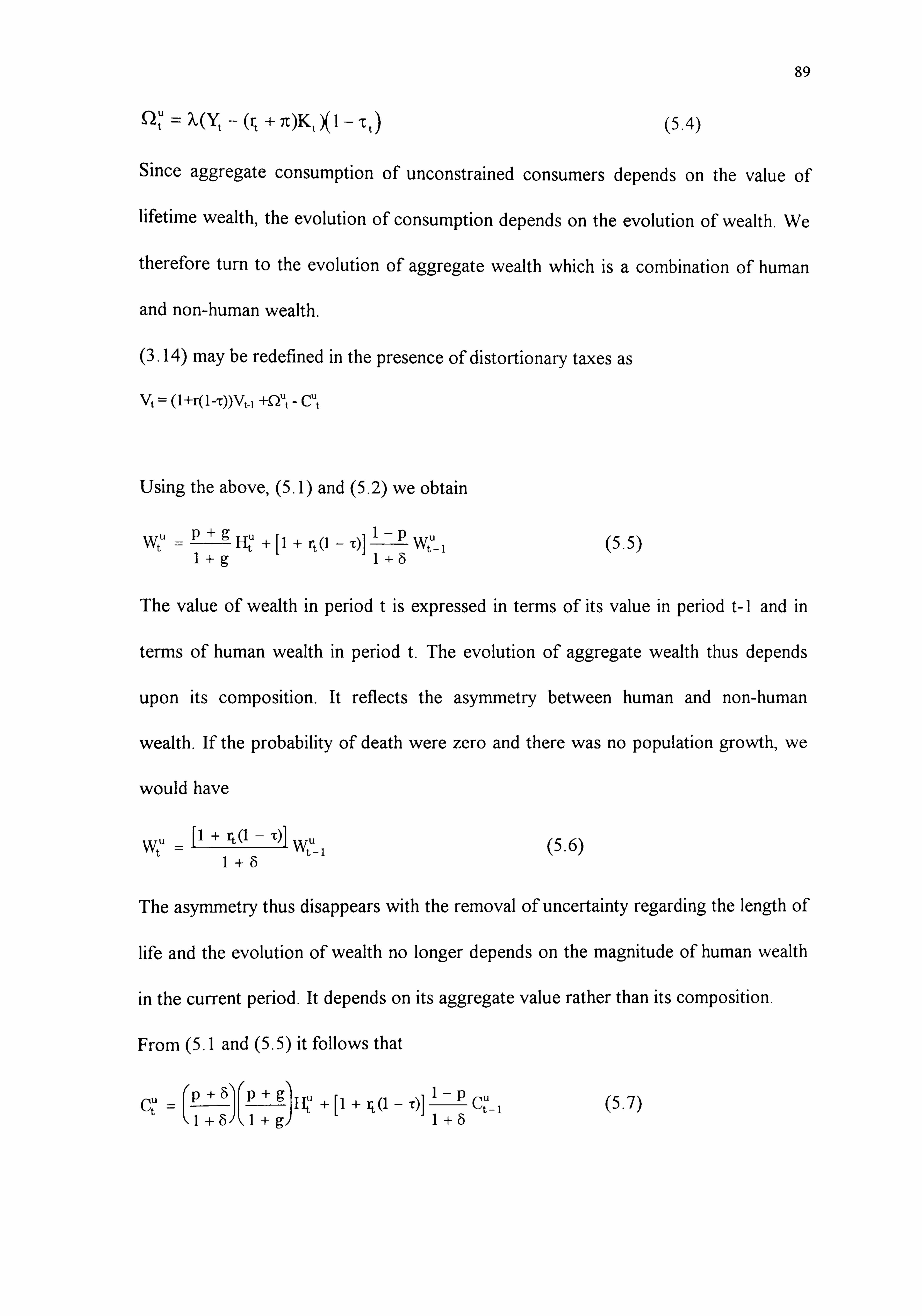
89

Qu t= ý-(Y, - (r, + Tj (5.4)

Since aggregate consumption of unconstrained consumers depends on the value of

lifetime wealth, the evolution of consumption depends on the evolution of wealth. We

therefore turn to the evolution of aggregate wealth which is a combination of human

and non-human wealth.

(3.14) may be redefined in the presence of distortionary taxes as

(I +r(I -r))V, -, +KY, - C',

Using the above, (5.1) and (5.2) we obtain

Wt" =p+9 fg ++ rt -C)] P wtu 1 (5.5)

1+g +6

The value of wealth in period t is expressed in terms of its value in period t- I and in

terms of human wealth in period t. The evolution of aggregate wealth thus depends

upon its composition. It reflects the asymmetry between human and non-human

wealth. If the probability of death were zero and there was no population growth, we

would have

P+ rt(i -u wtu -1 +6 vvt-1 (5.6)

The asymmetry thus disappears with the removal of uncertainty regarding the length of

life and the evolution of wealth no longer depends on the magnitude of human wealth

in the current period. It depends on its aggregate value rather than its composition.

From (5.1 and (5.5) it follows that

++ rt Q- -r)] IP Ct" (5.7) C tu 1 +5 t-I

90

If g=O , p=O , -c =0, and for a constant rate of interest, Ctu = I+ r Cu which I+g I-

corresponds to the Euler equation in the representative agent model with infinite

horizons. In addition if there are no liquidity constraints then aggregate consumption

Ct +r Ct_l . This shows that non-Ricardian behaviour of aggregate consumption

arises from four sources: finite horizons, population growth, distortionary taxes and

liquidity constraints. Effect on growth on each of these sources will be explored later.

Using (5.1) ), (5.2) and (5.5) we have

I+g u P+ö =[i+«I-T)] +-g

- TA Vt- (5.8) t t-1

+,. )(1 g)[i+«, l+8

-p which describes the consumption behaviour of the unconstrained consumers in terms

of lagged consumption and lagged non-human wealth. This may be referred to as the

discrete time Yaari-Blanchard consumption function. '

5.3.2. Private Sector Output and Investment.

The representative firm f produces homogeneous output with the following Cobb-

Douglas constant returns to scale production function at time t

Y =F(K,, f, J,, f)=K"t, fJ I-cc t'if t1f (5.9)

where K, rf is private physical capital and J, f is labour input in efficiency units. Or,

Jt, i et, iLt'i (5.10)

where F, ,f is a measure of the efficiency of raw labour input Lt. The crucial

assumption that drives endogenous growth in this model is that this efficiency measure

is a function of the economy-wide capital-labour ratio . Let Kt be aggregate private

For small r, g, p, X and 6 this corresponds to the C= (r-8)C - (p+g)(p+5)V in continuous time.

91

capital. In addition to the externality from private capital, the government affects

labour efficiency by providing physical capital in the form of infrastructure which may

be broadened to include education, health, etc., accumulated out of the economy's

single output. This is captured by

& t, f Ai

(K) (K) 1-y,

L (5.11)

where KG, is public capital and yj is the contribution of public capital to the economy-

wide efficiency of labour. This way workers inherit the benefits of past investment.

Assuming identical firms that are constant in number, and aggregating, we arrive at the

aggregate production function

y2G 1-Y2 Yt =

ýKý) (K t) (5.12)

where Y2=1- (1-(x)yl and B depends on the constant number of firms in the economy.

It is assumed that the government does not produce. It buys output, including

roads, dams, canals, hospitals, schools etc., from the private sector. This infrastructure

is made available to the private sector without any user charges. Private capital has a

a2yt t- <0. However, if the dirninishýing marginal product given by

aK2 t 'Y2(1 - yj)%

t Kt

ratio of public to private investment remains constant, i. e. with every increase in

private investment there is a corresponding increase in public investment, then the

marginal product of private capital is constant and is equal to its average product. The

average product of capital may be expressed as

yt =BG.

) 1-Y2

(5.13) Kt t

92

If the ratio KG'

is a constant then the production function displays constant returns to Kt

the input private capital and technology is linear .

Also, if yj=O i. e. public expenditure

has no role to play in raising the efficiency of labour then YT"ý1 and the production

function can be expressed as Y=BKt as in Romer (1986) where B>O is the constant net

marginal product of private capital. Technology in this case is linear.

We assume that firm f ignores the externality in choosing capital stock. The

marginal product of capital is NVK= DY/, DK = (xK'-' J'-' = (xY/K. The marginal cost of

capital (including depreciation at a rate 7r)=rt+7r. Equating the private marginal

product of capital to the cost of capital gives

Kt (X --= K(r)

Yt rt + 71 (5.14)

Net private investment is then given by the addition to capital stock less the

depreciation in period t

It = Kt - (I - Tr)Kt-, (5.15)

5.3.3. The Government

The government provides an amount Gc, of public consumption goods using the

same technology as for the privately produced good, and purchases an amount GI, of

the latter to invest in infrastructure. Total government expenditure is then

Gt = Gct+Gl, which is financed by a combination of taxation (Tt) and borrowing (D, )

where D, are single period bonds. (We ignore or rule out seigniorage). The

goverrurnent borrowing identity is given by

93

Dt = (I + rt)Dt -I + Gt - Tt (5.16)

and public sector capital accumulates according to

n)K G1+ Gtl t- (5.17)

assun-ung the same depreciation rate as in the private sector. Since the defiru I of

capital is broad, public sector investment GIt is assumed to include public expenditure

on health, education, etc. Since only profits net of depreciation are taxed at the rate T

total receipts are

Tt=-c (Yt-7cK, ).

5.3.4. Output Equilibrium.

We assume that the market always clears. Equilibrium in the output market gives

Y =C +1 +G tttt (5.19)

Thus, given the government choice of fiscal policy variables Gct, GI, and T, the supply

and demand sides of the economy are now fully determined.

5.3.5. The Steady-State

We seek a balanced growth steady-state in which all stocks and flows are growing

at the same enclogenous rate n, the steady-state value of nt. The debt/GDP ratio is

assumed to be constant which is the strong solvency condition. It is assumed that rt is

constant at the rate r. If we express all macroeconon-iic stock and flow variables as

ratios of GDP then in steady state balanced growth the ratios remain unchanged. We

retain the same notation without the subscript t to denote these ratios to ease

notational burden.

94

Consumption of constrained consumers who receive only labour income and

consume their entire income is given by

(r+ 7c)K, XI

- -c (5.20)

We can substitute for the expression for non-labour income from (5.14) where Kt(r+Tc)

Post-tax labour income of unconstrained consumers can be now defined in

terms of total income. Consumption of constrained consumers defined as a ratio of

GDP in the steady state is

ýtc =c =(I-k )(I-CCXI--c yt

(5.21)

We can now obtain the consumption of unconstrained consumers in the steady state

from

(p+g)(p+5)[1-r(I-t)]/(I-p))(D+K)

(5.22)

The capital output ratio may be expressed as a ratio of GDP as

K(r) = oc /r+Tc (5.23)

Given that the rate of depreciation for public capital is the same as that for private

capital we obtain public capital in the steady state as a ratio of GDP as

(I + n)Gl (5.24) (n + 7E)

where G1 is the share of public investment in GDP.

The aggregate production function can be expressed as a ratio of GDP as

G' 0 log B+

*y 2 logK+ (1 - Y2)109- (5.25) (n +7r)

95

In the steady state public and private capital grow at the same rate n and depreciate at

the same rate 7r. Thus the ratio of public to private capital is constant and so

production is linear in private capital.

In a steady state public debt grows at the rate n. Thus the government budget

constraint may be expressed as

(I+n)Dt = (I+r)Dt-I + Gt -Tt (5.26)

Rearranging, we express the solvency condition in the steady state as

[(r-n)/(I+n)]D =T -G =[1-7cK], c -G (5.27)

The market equilibrium in the steady state may be defined as ratios of GDP as

I=C'+C'+l +G

--c)-[(n+7c)/(l +n)]K(r)-G (5.28)

To summarise the steady-state form of the model may be expressed as

[1-r(1-t)J/(1-p)} (D+K)

[(r-n)/(l+n)]D=T-Cx--(1-7cK(r)), u-G

K=a / r+7c=K(r)

logB+Y2 log(K(r))+(I-Y2)log(yGI(n+n))ýO

cu=l-[(n+7c)/(l+n)]K(r)-G-(I-X) (1-a)(l-, c)

(5.22)

(5.27)

(5.23)

(5.25)

(5.28)

(5.21)

(5.22) defines the aggregate consumption of the group of unconstrained consumers.

(5.27) is the solvency condition of the government in the steady state. It is the strong

solvency condition which implies that the debt/GDP ratio is constant. (5.23) and (5.25)

96

describe the supply side of the model. (5.23) defines the steady state capital output

ratio. (5.25) defines the production function. (5.28) is the market equilibrium

condition. Together these define consumption, the government budget constraint,

production and market equilibrium in the steady state.

Futagan-ii, Morita and Shibata (1993) who assume externalites arising from the

stock of public and private capital on the supply side and from distortionary taxes on

the demand side find that the steady state equilibrium path is unique and exhibits

saddlepath stability. In a model of overlapping generations and enclogenous growth

where externalities on the supply side arise from the stock of capital and on the

demand side due to finite horizons, Alogoskoufis and van der Ploeg (1991) also find

that the steady state equilibrium is saddlepath stable. The condition of solvency of the

public sector is sufficient to ensure saddlepath stability. Corresponding to this

boundary condition there is a single value of the forward looking variable -

consumption at some initial time for which the system converges to a steady state. For

all other initial values of consumption we have explosive behaviour. Strictly speaking,

the stability of the steady state equilibrium in our model can be examined by linearizing

around the steady state and investigating the transitional dynamics. However, since our

model is later shown to be near Ricardian,, it is very close to Futagami, Morita and

Shibata (1993) and so we can draw upon their results and assume that the system will

exhibit saddlepath stability.

5.4. Fiscal Policy and Long-Run Growth

This section studies the steady-state of the economy defined above. Given fiscal

instruments, -c, GC and GI we have five equations In five endogenous vanables

97

r, C,, D,, K and growth n. Since we wish to focus on the effects of government debt D.

the distortionary tax rate -c, and the mix of government spending as between

consumption and investment, we will characterise fiscal policy in terms of D and -i

making total government spending endogenous. Let GI=yG making the third fiscal

instrument the proportion y.

To compute an "order of magnitude feel" for their effects on long-run growth we

derive multipliers for estimating the change in the rate of growth when there is a

change in fiscal policy variables.

Substituting the value of consumption and eliminating G we arrive at the Yaari-

Blanchard consumption relationship.

f(n, r, D, -c)=((I+g)(r(l--c))+g-5-n(1+6))(l-[(n+7c)/(l+n)]K(r)

+ [(r-n)/(1+n)] D-t(1-itK(r)-( 1-?. )( 1-r)(1-a)))

-I(p+g)(p+6)[l+r(l-, u)]/(I-p))(D+K(r))=O (5.29)

The production function may be derived as

g(n, r, D919Y)ýY21ogK(r)+(I-Y2)(109Y+109('E(I -nK(r)- [(r-n)/(I+n)] D)+Iog(l+n)-

log(n+-K)) +IogB=O (5.30)

The two relationships determine r and n given D, -c and y.

The relationship f(n, r, D,, r)=O describes the locus of interest and growth rates

consistent with Yaari-Blanchard consumption behaviour, output equilibrium, private

sector investment and the government budget constraint. We term this locus the Yaari-

Blanchard (YB) curve. The relationship g(n, r, D,, r, y)=O is the locus consistent with

balanced growth and our linear technology, private sector investment and the

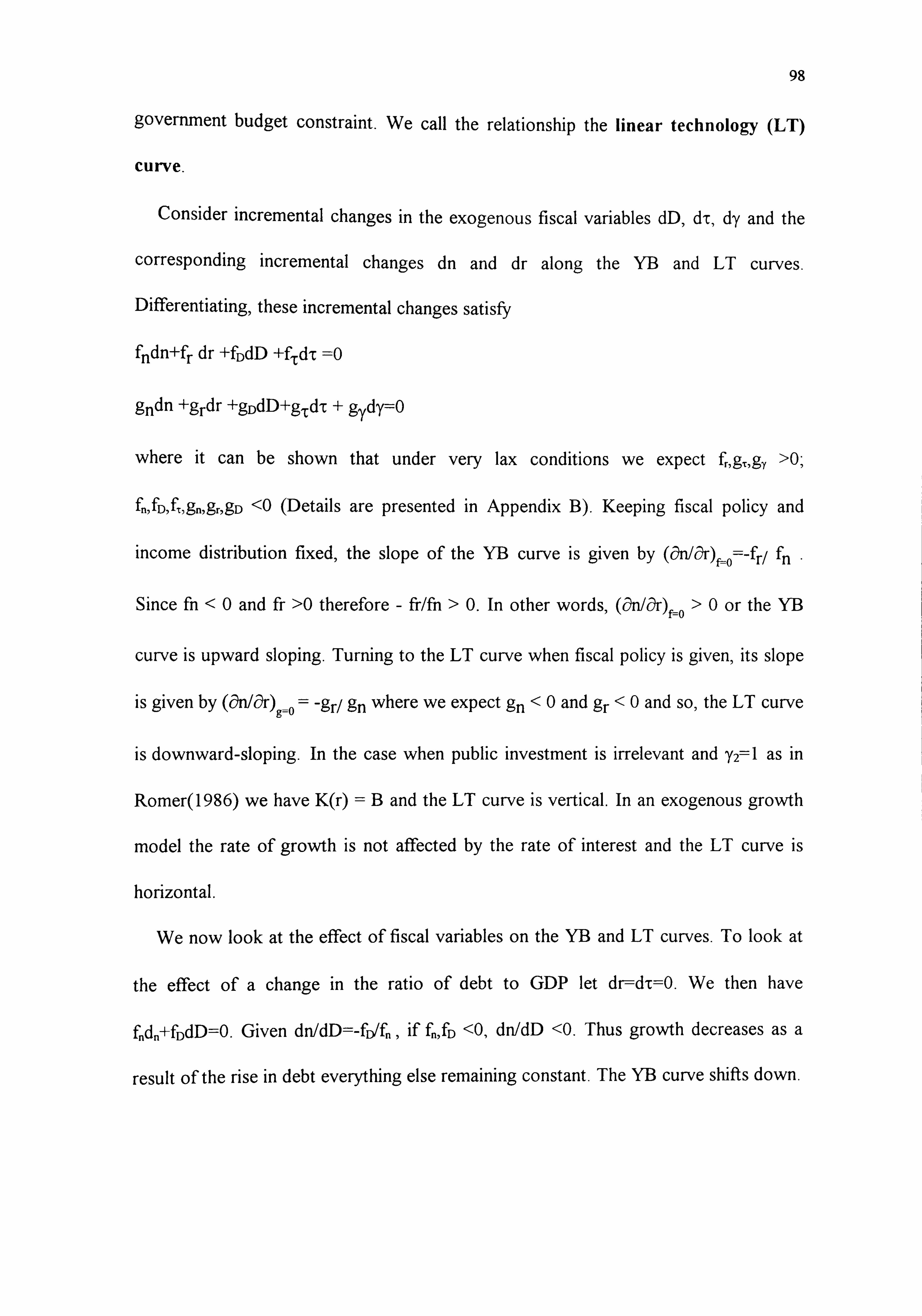
98

goverment budget constraint. We call the relationship the linear technology (LT)

curve.

Consider incremental changes in the exogenous fiscal variables dD, dT, dy and the

corresponding incremental changes dn and dr along the YB and LT curves.

Differentiating, these incremental changes satisfy

fndn+fr dr +fDdD +fcdz =O

9ndn +grdr+gDdD+grd-c + gydy--O

where it can be shown that under very lax conditions we expect f,, g,, g, >01

fn, fD, fc, gn, gr, gD <0 (Details are presented in Appendix B). Keeping fiscal policy and

income distribution fixed, the slope of the YB curve is given by (c-'n/c9r)f-O=-f r/ fn

Since fn <0 and fr >0 therefore - fr/ffi > 0. In other words, (cn/or)f-o >0 or the YIB

curve is upward sloping. Turning to the LT curve when fiscal policy is given, its slope

is given by (an1&)g=O = -gr/ gn where we expect gn `ý 0 and gr `ý 0 and so, the LT curve

is downward-sloping. In the case when public investment is irrelevant and Y2: --": l as in

Romer(1986) we have K(r) =B and the LT curve is vertical. In an exogenous growth

model the rate of growth is not affected by the rate of interest and the LT curve is

honzontal.

We now look at the effect of fiscal variables on the YB and LT curves. To look at

the effect of a change in the ratio of debt to GDP let dr--d-c=O. We then have

f. d,, +fDdD=O. Given dn/dD=-fl)/f,, if f., fD<O, dn/dD <0. Thus growth decreases as a

result of the rise in debt everything else remaining constant. The YB curve shifts down.

99

Similarly, keeping r, -c and y fixed, dr--d-c=dy=O, we have gndn+gDdD=o and so dn/dD=-gE'/gn

-If 9D, gn<O then dn/dD<O and the LT curve shifts downwards when debt

increases. The combined effect of an increase in debt is a reduction in long-run growth.

The Yaari-Blanchard and Linear Technology Curves :

Effect of a rise in the Debt/GDP ratio

rate of growth

n

r rate of interest

Figure 5.1

We can derive the debt/GDP ratio multiplier

[aNADD] g, fD-gDf gf r' frgn-

rn

wherefrgn-g f<0. From the expected signs of the partial derivatives we can expect rn

to be negative. This implies that an increase in the steady state ratio of public

debt to GDP reduces long-run growth given the ratio of government consumption to

government spending and the tax ratio. This effect is not contrary to our expectations

100

in a non-Ricardian world. Since public debt is considered net wealth in such a world,

an increase in debt would raise consumption spending and reduce private savings

available for investment. It should thus have a growth reducing effect if long-run

growth depends on the level of investment.

Let us now look at the effect of a change in the tax rate. We assume that dr--dD=O.

Now, f,, dn+fd-c=O or dn/d-c=-f, /f,,. If f, f,, <0 as expected, dn/dT <0. In other words

when the tax rate increases less is available for private sector saving and investment

and when investment is lower, the growth rate is lower in an endogenous growth

model. Hence the YB shifts down.

To look at what happens to the LT curve, let dr--dD=dy--O. We have g. dn+g, d-c=O.

So, dn/d-c=-g, /g,,. If g, >O, g,, <O then dn/dc >0. The LT curve shifts upwards when the

tax rate increases. This is because more can be invested by the government while

satisfying its intertemporal budget constraint. The total effect of the change in tax rate

in not clearly in any one direction. We can derive the tax rate multiplier as

gf [G-N/O']D, y 7--g, fr-gTfr / fr9n- r n.

While the denominator is negative, the numerator can be either positive or negative.

An increase in taxes thus has an ambiguous effect on growth. The reason for this is

that as the tax rate increases, given the debt/GDP ratio, a higher government spending-

GDP ratio consistent with the government budget constraint can be reached. Part of

this additional spending goes on infrastructure which enhances growth. However, taxes

are distortionary and, for a given real interest rate r, an increase in the tax rate reduces

savings as a proportion of GDP which depresses private investment and hence growth.

Let us now look at the effect of the third fiscal policy variable y. Since YB is not a

function of y, it does not shift due to a shift in y. On the LT curve we assume that the

101

tax rate and debt/GDP ratio remaining constant we will have dn/dy---gýgn- If g, >O and

g. <O then dn/dy >0. The LT shifts upwards. An increase in the proportion of

government spending on infrastructure raises the growth rate. We can show

113N119'YID, -c '- gyfr / frgn-grfn >O

The result that an increase in the proportion of government spending on investment

and development purposes raises growth is again in accord with the basic

characteristics of the growth model presented here.

5.5. Calibration and estimation for India

In this section we present the data used and the results obtained. We use the values

of parameters on the demand side as in the previous chapter to calibrate the above

model. Other observed variables are those reported in the Economic Survey 1993-94,

Government of India and Yearbook of the International Financial Statistics published

by the International Monetary Fund.

We assume that r. the implicit risk free real interest rate relevant for consumption

decislons, is 14.16 per cent, the proportion of labour income received by unconstrained

households is 70 per cent, the probability of death, p, is 0.019 and 6, the rate of time

preference, is 0.032.

The Economic Survey 1993-94 reports a rate of growth of population over 1981-91

to be 2.14 per cent. GDP grew at an average rate of approximately 4.5 per cent over

this decade. Gross Domestic Private Investment as a percent of GDP for 1991-92 is

reported to be 14.0 per cent. Consumption as a percent of GDP is calculated to be 64

per cent ftom the figures provided by the IW. Government spending constitutes 22

per cent of GDP. The total outlay of the government - Central and State Governments

II 0-

and Union Territories is categorised as development and non-development

expenditure. Non-development expenditure includes defence, tax collection charges,

police, etc. To analyse the impact of government spending on productivity, we choose

y to be development expenditure as a proportion of total government expenditure.

This includes public investment in infrastructure, education and health. Table 1.5

shows that development spending as a proportion of total government expenditure has

declined by about 10 per cent in the last decade. and was 54.3 per cent in 1993-94.

Table 5.1: Summary of Calibration.

Sources

Parameter Value

Depreciation Rate =n0.05

Real Rate of Interest =r0.14

Rate of time preference =60.032

Consumption/GDP =C0.64

Gov. Exp. /GDP =G0.22

Gov. Debt/GDP =D0.60

probability of death p 0.019

liquidity parameter X 0.70

rate of growth of population =g 0.0214

GDP growth =n 0.045

Development Exp. /Gov. Exp. =y 0.543

Capital Extemality =yI

Y2 1-(1-a)yi

Economic Survey, Government of India, (Various issues), Annual Report,

Reserve Bank of India, Bombay.

-x, the rate of depreciation, is chosen to be 5 per cent. Depreciation of physical

capital through technological obsolescence as well as wear and tear may be expected

to be roughly 10 per cent. Our concept of capital is broader and includes human as

103

well as physical capital. Since we expect a much lower depreciation rate for human

capital we choose the average depreciation rate for our broad concept of capital to be

5 per cent.

yj is the contribution of public capital to the production externality i. e., it is the

contribution of public capital to the economy-wide efficiency of labour. As yi is neither

estimated nor observed, it is imposed. Since we do not know its value, we impose

different values of yj and calibrate the model. To each level of yj corresponds I-Y2 ý'Yl

(1-cc), the elasticity of aggregate output to public capital stock. The value of cc, the

share of income accruing to private capital, was revealed to be approximately 29 per

cent. So the higher is yi the higher is the elasticity I-Y2.

The marginal products of private and public capital can be shown to be Y2(Y/K) and

(I -Y2) (Y/ KG). Since the ratio of both public and private investment to GDP is each

approximately II per cent, the marginal product of private and public capital may be

compared by comparing the value Of Y2 to (1-Y2)- If Y2 ýI-Y2 i. e. Y2": --0.5, the two

marginal products are equal and output cannot be increased by reallocating resources

from the public to the private sector or vice versa. Our calibration shows that (x=0.29

and Y2=--I-Y2 when y1=0.7. Allocation of capital between public and private sectors is

then efficient. If (1 -72 )< 0.5 output can be raised by reallocating investment from the

public to the private sector then size of the public sector is too large. The Table 5.2

shows the values of the multipliers when the model is calibrated at different values of

Yi.

104

Table 5.2: The Multipliers for selected values of yj

Yl O)IVO'y cýtVaD an/&T

0.2 0.03232 -0.00497 -0.0625 0.5 0.07678 -0.01202 0.06384

0.7 0.10404 -0.02174 0.14130

0.9 0.12960 -0.02772 0.21393

5.5.1. The Development Expenditure Multiplier

The development expenditure multiplier, (o-'nl&y), measures the change in long run

steady state growth rate corresponding to a change in the proportion of development

expenditure in total government spending when the tax rate and the debt /GDP ratio

are unchanged. For yl=0.2 a one per cent increase in the proportion of development

expenditure in government spending leads to an increase in the long-run growth rate by

0.03 per cent. Similarly if yj were 0.7 the rise in the long-run growth rate would be 0.1

per cent. A ten per cent reduction in the proportion of development expenditure then

implies aI per cent decline in the long run growth rate.

105

yl and the development expenditure multiplier

0.14 cu 1- 0.12 Z

0.1

0.08 Cu 0. ýw Z; or- 75 0.06 EE 0.

0.04

0.02 *0

cleveloýment expenditure multiplier

0 C4 Cf) 'RT LO (0 r- 00 0')

ci ci C: ) C=; 6 C; C=; C;

71

Figure 5.2

Any increase in the proportion of public investment to total government spending

raises the long-term growth rate whatever the efficiency of the public sector. However,

when yj is higher, a reduction in the ratio of development expenditure to total

government expenditure reduces growth to a larger extent. This can be seen in Figure

5.2. The higher is yi, the contribution of the public sector to raising the economy-wide

efficiency of labour, the greater is the effect on long-term growth of a reduction in the

proportion of public investment to total government spending.

5.5.2. The Tax Multiplier

While growth rates unambiguously increase as debt declines or as government

spending on infrastructure increases, other things remaining the same, the change in

growth brought about by a change in the tax rate is not so well defined. The tax

multiplier, (anlar), measures the change in long-run steady state growth due to a

change in T, the tax rate, when D and y are unchanged. Given the government budget

106

constraint a rise in the tax rate allows higher public spending and thus investment.

When yj is high, then a rise in the tax rate which reallocates resources to the public

sector raises long-term growth rate. The tax multiplier is therefore positive. However,

when yj is low, higher taxes imply an increase in public investment at the cost of

private saving which leads to a reduction in private investment. An increase in tax rate

reduces long-run growth rate when the contribution of the public sector to the growth

potential of the economy is relatively lower.

0.25

0.2

0.15

0.1

0.05

0

-0.05

-0.1

-0.15

yl and the tax multiplier

I -tax multiplier ý

CN c4-) le L£) (0 r- 00 0)

yl

Figure 5.3

Figure 5.3 shows how the value of the tax multiplier rises with an increase in yi. We

see that the sign of the tax rate multiplier changes from negative to positive as yj rises.

5.5.3. The Debt Multiplier

The debt multiplier, (65'n/aD), measures the change in long-run steady state growth

due to a change in D, the debt/GDP ratio, when 'r and y are unchanged. Table 5.2

107

shows that if yi were 0.2, a one per cent increase in the debt/GDP ratio leads to a

reduction in the long run growth rate by 0.005 per cent. Or, a hundred per cent

increase in the debt/GDP ratio would reduce growth rate by 0.5 per cent. At yl=0.7 a

hundred per cent increase in D would reduce the growth rate by 2.17 per cent.

, yl and the debt multiplier

0 c114 CY) le LO (0 r, - OD

c; c; ci ä c; -0.005

-0.01

-0.015

-0.02

-0.025

-0.03

debt multiplie

YI

Figure 5.4

We observe in Figure 5.4 that the absolute value of the multiplier rises when yj Is

higher and a rise in the debt ratio reduces long-term growth to a larger extent. If taxes

remain unchanged, then a reduction in debt is achieved by reducing government

spending. Since development expenditure constitutes nearly half of total government

spending, the higher is yl, the larger will be the effect of a reduction in debt on long-

term growth rate.

As discussed in detail earlier, the ratio of development expenditure in the

government's total expenditure is rapidly declining in the face of the commitment to

108

reduce public borrowing under the SAP. Our calibration suggests that the effect of the

decline in the ratio of development expenditure on the growth rate is quite significant. 17) Assuming a mean level of yi, reducing the proportion of development spending from

the present y=54.3 per cent say by another 10 per cent to 44.3 per cent, keeping the

tax rate and the debt/GDP ratio unchanged, will reduce growth by more than 0.7 per

cent. The pattern of government spending therefore has a significant effect on the long-

run growth rate of the economy. For, instance if half of defence expenditure, which is

about 20 per cent of total government spending, was diverted to development

purposes y would increase from 54.3 to 64.3 and the long-run growth rate would rise

by about 0.76 per cent.

A 0.5 per cent increase in growth could be achieved either by a less than 10 per cent

rise in the ratio of development expenditure in total expenditure or by a 50 per cent

reduction in the debt/GDP ratio from the present 0.6. The second is much larger in

magrutude. Since total government expenditure stands at about 22 per cent of GDP

and slightly more than half of it is development expenditure, development expenditure

stands at about 12 per cent of GDP. Thus higher growth to the same extent could be

achieved by a small increase in development expenditure rather than a large reduction

in debt.

The effect of small changes in more than one fiscal variable can be analysed as

follows. Since we have n=n(D, y,, r), the total effect is given by

NNN dn dD +- dy +- dT

. If the fiscal deficit Is reduced by rals'ng the tax rate, -c,

OD C'Y Cn-1

while the proportion of infrastructure spending to total government spending remains

109

unchanged, then the total effect on long term growth rate can be measured by

dn = cn dD +

an d-,.

c9D aT

On the other hand, the tax rate could be kept constant and the fiscal deficit could be

reduced by cutting public spending. Government expenditure can be reduced either by

a reduction in both consumption spending and investment such that y remains

unchanged, or by a reduction in one such that y changes. If, say, the reduction is

brought about by a cut in the expenditure on infrastructure, because of which y

changes, the total effect on growth would be dn = on dD +

an dy

. Here the first term aD Cly

is positive since debt has been reduced and the second term is negative since there is a

fall in y which reduces growth. The total effect on growth depends on which effect is

larger.

5.6. Non-Ricardian Effects

In this section we examine some of the implications that arise from the violation of

Ricardian assumptions. We first look at the values the tax and debt multipliers would

take on if the planning horizons of the unconstrained consumers were different. We

next look at the effect of liquidity constraints.

5.6.1. Finite horizons

If the probability of death is higher the effect of the shorter time horizon on the

consumption of unconstrained consumers is revealed as larger non-Ricardian effects on

growth rates. Figure 5.5 shows that the absolute value of the debt multiplier increases

as the probability of death approaches unity. This accords well with our expectation

110

that if consumers have shorter planning horizons then public debt is treated as net

wealth and consumption rises crowding out private investment and reducing the rate of

growth in our model. When p=O the value of the multiplier is non-zero because of

other non-Ricardian effects, namely distortionary taxes, population growth and

liquidity constraints and the public capital externality.

Finite horizons and the debt multiplier

-o. c

-0

75 E

-0.1

-0

-0.25

p=the probability of death

Figure 5.5

Similarly the value of the tax multiplier would be higher if the probability of death

were higher. Shorter time horizons represented by a higher value of p, other

parameters remaining the same, imply small changes in the tax rate would have much

larger effects on growth. Again the multiplier is non-zero when p=O because of other

non-Ricardian effects. This can be seen in Figure 5.6.

ill

0.6

Finite horizons and the tax multiplier

0.5

0.4 CL

0.3 E x 2 0.2

0.1

0

---7 ax multiplier,,

C) 04 CO Ict LO (D r- 00 (3)

ci C) 66C; C) C) C; p=the probabilitY of death

Figure 5.6

5.6.2. Liquidity constraints

We now examine the effect of liquidity constraints on the tax multiplier.

As Figure 5.7 shows the value of the tax multiplier falls as we approach the Ricardian

case (k=l). This is because if a higher proportion of income is received by forward

looking consumers then the effect of a change in the tax rate on consumption will be

lower and the magnitude of crowding out is smaller. Hence the effect of a change in

the tax rate on the growth rate is smaller.

112

0.08

Liquidity constraints and the tax multiplier

0.07

0.06

U. 05

75 0.04 E x 0.03

0.02

0.01

0

ix multipli

C) - CN 00 qt LO (D t-- 00 CF) 666C; C=; CD C) Ci Ci

the proportion of income received by unconstrained consumers

Figure 5.7

5.6.3. Distortionary Taxes

To examine the effect of distortionary taxes we assume that p=g=O and k=l as in

the Ricardian case. Now the deviation from Ricardian Equivalence is due only to

distortionary taxes and the public capital externality. We re-estimate the multipliers

at the mean value of yj = 0.5. Table 5.3 shows us how these 'quasi-Ricardian'

multipliers compare with the non-Ricardian case when there exist finite horizons,

population growth, liquidity constraints and distortionary taxes. Since the

development expenditure multiplier is determined on the supply side of the model we

look at the tax and debt multipliers which would be affected by non-Ricardian effects

on demand.

113

Table 5.3: The Multipliers for the Quasi Ricardian and Non-Ricardian Cases

Multiplier Quasi Ricardian Non-Ricardian

cýlvaD -0.0154 -0.0153

Cýn/c't 0.0599 0.0638

The tax and debt multipliers in the Quasi Ricardian case are only marginally

lower than in the non-Ricardian case. Clearly the effect of finite horizons, population

growth and liquidity constraints is not very large. We examine the relation between the

tax rate and the long-run growth rate in Figure 5.8,5.9,5.10 and 5.11. We also look

at the choice of the tax rate that maximises growth. This is considered to be the

coptimal' tax rate.

We first examine the relationship between the tax rate and the growth rate in

Figure 5.8. yj is assumed to be the mean level of 0.5. Figure 5.8 shows the optimal tax

rate for different levels of y, the ratio of development to total government spending.

Given the level of y at 0.54 growth rate can be raised by raising the tax rate to about

40 per cent. If y were higher by 10 or 20 percentage points, growth rates achieved

would be relatively higher at any tax rate.

114

Growth, Tax Rate and Development Expenditure

0.09

0.08

0.07

0.06

0.05

0.04

0.03

I-Iolo,

0.02

0.01

y=0.54

y=0.64

Y=0.74 0

0.2 0.3 0.4 0.5 0.6 0.7

Tax rate

Figure 5.8

As discussed earlier the effect of distortionary taxes on the long-run growth rate

depends on the contribution of public capital stock to the economy wide efficiency of

labour. We see that the optimal tax rate is different at different values of yi. Figure 5.9

indicates that if yj =0.25 the maximum growth rate is achieved when the tax rate is

around 25 per cent. The higher is yi, the higher is the optimal tax rate. When yj =0.75

the optimal tax rate is around 57 per cent.

115

Growth, Tax Rate and Yl

0.08

0.07

0.06

0.05

0.04

(9 0.03

100.00

1

000, IN

0.02

0.01

-yl=0.25

--- yl=0.5

------- yl--0.75

0 4-

0.2 0.3 0.4 0.5

Tax Rate

Figure 5.9

0.6 0.7

Figure 5.10 shows growth rates at different levels of the tax rate corresponding to the

debt /GDP ratio. yj is assumed to be the mean level of 0.5. Again growth rate can be

increased from its present level by raising the tax rate up to about 40 per cent. If the

debt/GDP ratio is lower then growth rates are relatively higher for all -c.

116

0.08

0.07

0.06

0.05

0.04

0.03

0.02

0.01

0

Growth, Tax rate and the Debt/GDP ratio

/�

D=0.4 D=0.5 D=0.6

0.2 0.3 0.4 0.5 0.6

Tax Rate

Figure 5.10

0.7

Finally Fig. 5.11 shows the optimal tax rate for different values of the liquidity

parameter k. It also shows that the effect on growth of changing the proportion of

income received by unconstrained consumers. It can be seen that this effect is quite

small. Increasing the proportion of income earned by the rich will not increase growth

substantially even though they save and the poor don't. If all post-tax labour income

was to be received by unconstrained consumers ( ?, = 1), the long run growth rate

would be about 0.2 per cent higher. For the present value of the liquidity parameter of

70 per cent, the optimal tax rate is about 40 per cent. This is not sigruficantly affected

by the value of X.

117

Liquidity Constraints and Growth rate

0.08

0.07

0.06

0.05

0.04

0.03

0.02

0.01

0

. 00, - -- --------

". 0000

. 000, 100,

X=0.7

/X=0.4

0.2 0.3

5.7. Reducing Debt

0.4 0.5 0.6

Tax rate

Figure 5.11

0.7

The effect of a reduction in debt has been examined above by looking at the

change in the growth rate induced by small changes in the debt/GDP ratio. The

multipliers were derived at the current level of the debt/GDP ratio of 0.6. In Figure

5.12 and Figure 5.13 we observe that if the debt/GDP ratio was considerably reduced

then the development expenditure and the tax multiplier acquire much higher values. A

small increase in the proportion of development expenditure in total government

in the tax rate can raise the long-run steady state growth rate spending or an increase II

more effectively at lower levels of the debt/GDp ratio.

118

0.1

The debt/GDP ratio and the tax 0. - '. IlluiLlpilul

0.09

0.08

0.07

U. uo 0.05

0.04

0.03

0.02

0.01 I -tax multiplier ý

0! 11111i111 C) v-- CN c1f) 44, U) (D r- 00 0)

ci C; C; 6 C) C=i ci C; C;

DebVGDP

Figure 5.12

The debt/GDP ratio and the development expenditure multiplier

0.084

0.082

0.08

0.078 CL x U. Utb

0.074 EE CL 0.072

0.07 CD

,a0.068

0.066

- development expenditure multiplier

0 clq le (0 00

c; c; c; Debt/GDP

T-

Figure 5.13

119

5.8 Effects of Demand and Supply Side externalities

In this section we impose restrictions on the parameters p, g, k, -c and yj to

evaluate the relative importance of the non-Ricardian effects for empirical analysis and

obtain a range of specifications including the 'pure' Ricardian, and models similar to

Alogoskoufis and van der Ploeg (1990) and Buiter (1991) among others. The

endogenous growth character of the model is retained throughout by the assumption

that there are externalities arising from private capital.

In the 'pure' Ricardian case we assume that there are no public capital

externalities, no liquidity constraints, no population growth, horizons are infinite and

taxes are non-distortionary. So p=g= I- X= -i = yj = 0.

The aggregate consumption function can be shown to be

I+r Ct

1+(5 Ct-I

as in (2.9) which defined the consumption function of a representative agent. In the

steady state expressing consumption as a ratio of GDP

«1+n)(l+5)-(1+r»C =O

Since taxes are lump-sum, the government budget constraint is

G=T-(r-n)/(I+n)D

The market equilibrium condition is

+n) )K -

The 'Ricardian' equivalent of the 'Yaari-Blanchard' consumption function is

f(n, r, D) = ((I+n)(1+6)-(I+r))( I- ((n+7r)/(I+n) )K - T+(r-n)/(I+n)D) =

120

Assuming that yi =0 as in Romer (1986) i. e. public capital has no externalities then the

LT curve becomes

logB + log K(r) =

The debt multiplier has been defined as

[aNlaD] ` -r, y'- grfD-gDfr / frgn-grfn

In this case9D =0 and if n=r- 5, fDapproaches zero and the debt multiplier approaches

zero. The tax and development expenditure multipliers are also both zero. In other

words, when consumers have infinite horizons, there are no liquidity constraints, no

population growth, taxes are lump sum, public capital has no externalities and the

growth rate is equal to the real interest rate minus the pure rate of time preference,

fiscal policy is neutral.

In the Yaari-Blanchard case when only p#0, and we assume that there are no

liquidity constraints, population growth or externalities associated with public capital

and n= r-5, non-Ricardian effects arise as the probability of death is positive. Due to

finite horizons public debt is considered net wealth and this raises consumption and

reduces saving which in turn reduces net investment and hence reduces the long run

growth rate. The restrictions that g=0, X=1, -c = 0, yj =0 and n=r-5, reduce our

model to the Alogoskoufis and van der Ploeg (1990) specification. As can be seen in

Table 5.4 if p=0.02 we find that when taxes are lump sum, the value of the debt

multiplier is -0.0013. Thus a 100 percent decrease in the debt/GDP ratio leads to a

0.13 percent rise in the growth rate. Our result that in the presence of finite horizons, a

change in the debt/GDP ratio affects the long-run growth rate, corresponds with their

conclusions. When finite horizons and population growth are both included in the

model as in Alogoskoufis and van der Ploeg (1991) and Bulter (1991) the debt

121

multiplier becomes -0.00 18. In other words, if in addition to finite horizons we include

the population growth rate the absolute value of the debt multiplier rises by 0.0005.

This suggests that the effect of Blanchard-Weil demographics are significant when

taxes are lump sum and there arise no externalities due to public capital.

The model incorporates tax distortions in the form of a flat rate income tax

imposed on all labour and non-labour income as in Barro (1990) and Futagami, Morita

and Shibata (1993), Jappelli and Meana (1994) and Krichel and Levine (1995). When

none of the other Ricardian assumptions are violated the debt multiplier is found to be

non-zero at -0.001. The non-zero effects of government borrowing on long-run

growth are entirely due to distortionary taxes. We can again look at how the

multipliers would be affected if there one or more of the other assumptions of the

Ricardian theorem were violated as well.

When finite horizons and population growth are incorporated in the model with

tax distortions the absolute value of the debt multiplier becomes higher. At p=0.02, g

=0 the value of the debt multiplier is - 0.0027 and at p=0.02, g=0.02 it is -0.0030.

In comparison with the lump sum tax case these values are nearly double indicating the

importance of tax distortions. These results suggest that models like Alogoskoufis and

van der Ploeg (1990,1991) and Buiter (1991) while taking into account effects of

finite horizons and population growth on the demand side, ignore more important

demand side non-Ricardian effects due to distortionary taxes.

When the stock of public capital affects the economy-wide efficiency of labour,

the effect of fiscal policy on the long-run growth rate is due not only to non-Ricardian

demand side effects but due to the direct effect of public spending on infrastructure,

education, health and other development expenditure which creates physical and

122

human capital. We see that the multipliers are much larger in magnitude when the

externality arising from public spending is taken into account. Our results are

summarised in Tables 5.4,5.5 and 5.6. At yl=0.5 the tax multiplier is now positive

which indicates that higher taxes that finance public investment serve to raise growth,

outweighing negative demand side effects.

Table 5.4: The Debt Multiplier

Case Distortion Lump sum axes Distortionary Taxes Pure Ricardian None 0 -0.001 Finite Horizons p=0.02 -0.0013 -0.0027 Finite Horizons and p=0.02 -0.0018 -0.0030 Population Growth g=0.02 Public Capital yj = 0.5 -0.0065 -0.0061 Externality Finite Horizons and yj = 0.5 -0.0074 -0.0074 Public Capital p 0.02 Externality Finite Horizons, yj 0.5 -0.0078 -0.0079 Population Growth p 0.02 and Public Capital g 0.02 Externality Liquidity yj 0.5

3

-0.0088 Constraints, Finite k 0.7 Horizons, p 0.02 Population Growth g 0.02 and Public Capital Externality

2 We set r=0.077 so that n= r- 5. All other parameters retain their previous values. ' in the care when we have lump sum taxes and liquidity constraints \ke need to deterimne the share of taxes paid by the two gotips ot

consumers. Since there is no evidence for this we avoid imposing an arbitru-), value and so do not calculate this multiplier.

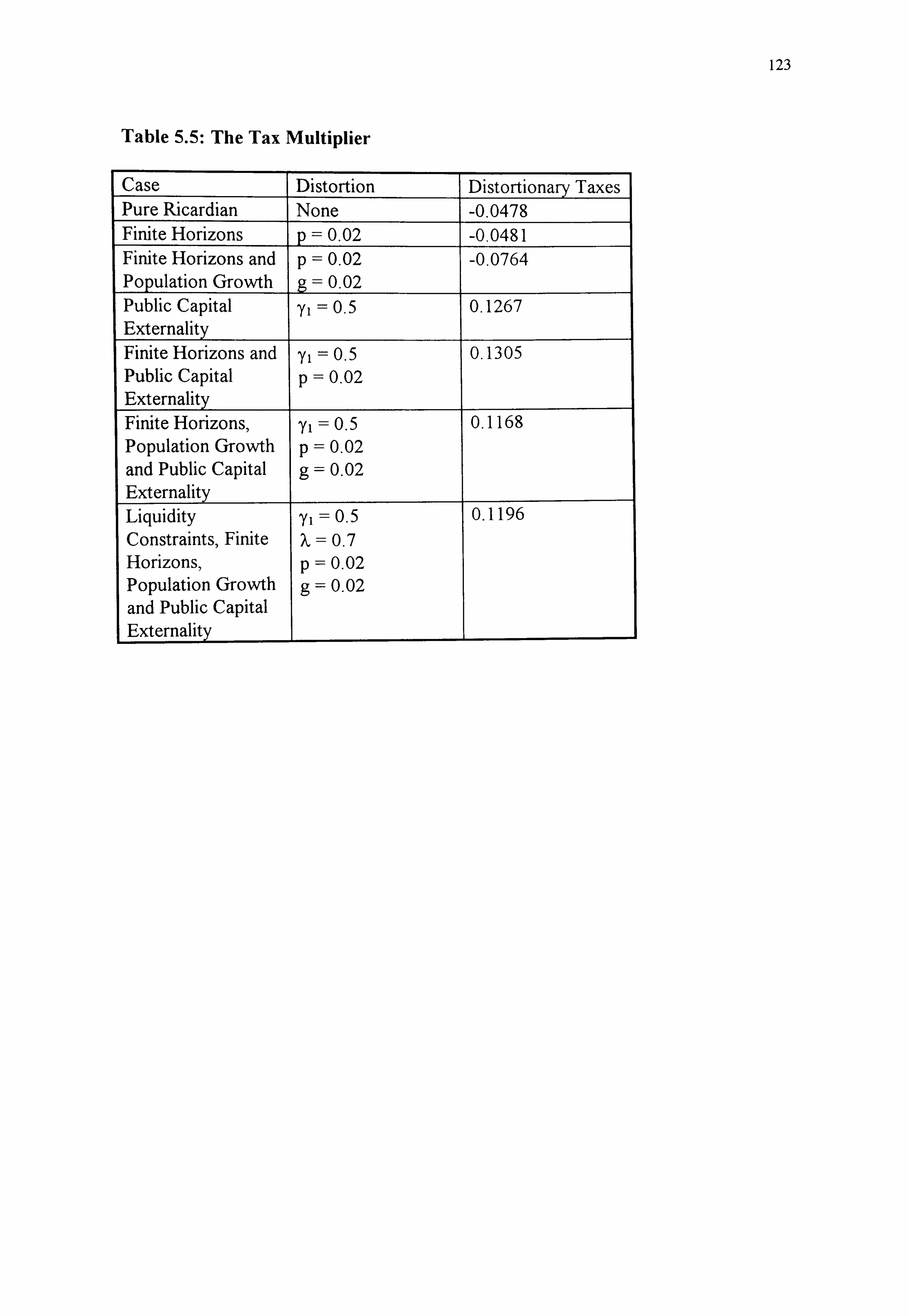
123

Table 5.5: The Tax Multiplier

Case Distortion Distortionary Taxes Pure Ricardian None -0.0478 Finite Horizons p=0.02 -0.0481 Finite Horizons and p=0.02 -0.0764 Population Growth g=0.02 Public Capital yj = 0.5 0.1267 Externality Finite Horizons and yj = 0.5 0.1305 Public Capital p 0.02 Externality Finite Horizons,, yj 0.5 0.1168 Population Growth p 0.02 and Public Capital g 0.02 Externality Liquidity yj 0.5 0.1196 Constraints, Finite ?, 0.7 Horizons, p 0.02 Population Growth g 0.02 and Public Capital Externality

124

Table 5.5: The Development Expenditure Multiplier

Case Distortion Lump sum Taxes Distortionary Taxes Pure Ricardian None 0 0 Finite Horizons p=0.02 0 0 Finite Horizons and p=0.02 0 0 Population Growth g=0.02 Public Capital yj = 0.5 0.0850 0.0710 Externality Finite Horizons and yj = 0.5 0.0858 0.0726 Public Capital p 0.02 Externality Finite Horizons, yj 0.5 0.0874 0.0754 Population Growth p 0.02 and Public Capital g 0.02 Externality Liquidity yj 0.5 0.0765 Constraints, Finite ?, 0.7 Horizons, p 0.02 Population Growth g 0.02 and Public Capital Externality

When we include only the externality due to public capital then the value of the

debt multiplier is -0.0065, while if we include all the non-Ricardian demand side effects

due to finite horizons, population growth, tax distortions and liquidity constraints it is

-0.0088. This means that the effect of a ten per cent reduction in growth rate would

raise the long run growth rate in the first case by 0.065 per cent and in the second by

0.088 per cent. By ignoring non-Ricardian demand side effects, though they have been

found to exist, the anticipated change in the long run growth rate would not be very

different. From the current level of 4.5 per cent it is anticipated to rise to 4.5088, when

demand side effects are included and 4.5065 when they are ignored. Even in the case

125

of development expenditure and the tax rate, there is only a marginal change in the

value of the multiplier when these effects are ignored.

The strongest effects arise from public capital externalities, and in their absence

from tax distortions. Our results thus appear to suggest that in an enclogenous growth

model which takes into account strong supply side effects caused by externalities

ansing from public investment, ignoring non-Ricardian effects on the demand side

would not significantly affect our results. Ignoring Blanchard-Weil demographics may

on the one hand lead to loss of generality and perhaps reduce the accuracy of our

results, but more may be gained by the analytical simplicity achieved by making

Ricardian assumptions on the demand side.

5.9. Conclusion

Our analysis reveals the significance of the violations of Ricardian assumptions. Our

results indicate that though non-Ricardian effects are potentially significant the effect

of population growth, finite horizons and liquidity constraints does not change our

results drastically.

The major policy implications that arise from the above results are that the growth

rate of the Indian economy can be raised most effectively by either raising the tax rate

or by raising the Proportion of development expenditure. The tax rate can be raised

effectively by bringing into the fold of the tax structure those sectors that at present

enjoy exemption. Rationalising the tax system while widening the tax base could be

more effective in raising the proportion of income that is paid as taxes. As we have

discussed earlier, there is an attempt to strean-dine, restructure and rationalise the tax

structure under the SAP.

126

On the other hand, there is no attempt to raise development expenditure. On the

contrary, y has declined in this period. Cutting public investment is going to reduce the

long term growth potential of the economy. Such a policy is counter-productive and

though there seems to be a general awareness of the implications of reducing public

investment, it is still being followed to meet the government's commitment under the

SAP to cut deficit. Clearly, the emphasis needs to shift from simply cutting the deficit,

to cutting it by reducing non-development expenditure and to diverting spending from

government consumption to public investment. Unless the policy framework of the

SAP clearly defines the role of public investment and takes into account the effect of

government Policies on long-run growth, borrowing countries concerned might

continue to follow such counter-productive policies. A clear definition of the role of

public investment and its contfibution to the economy wide efficiency of labour can

prove to be a step towards raising the long-run steady state growth rate in the

economy.

127

Conclusion

In this thesis we examine the effects of fiscal policy on the long-run steady state

growth rate in the fi7amework of an enclogenous growth model of India. We first exarnine

the Ricardian hypothesis that predicts that fiscal policy has no effect on consumption and

private investment in an economy. Next we estimate non-Ricardian effects on the demand

side and calibrate our model which has public capital externalities on the supply side to

determine the impact of changes in tax rate, debt /GDP ratio and the proportion of

government spending on development on the long-run steady state growth rate of the

economy.

Since Ricardian Equivalence predicts that fiscal policy is neutral we first examine

the Ricardian model for India. Underlying the Ricardian equivalence theorem is the

permanent income hypothesis and the assumption that there are no credit market

imperfections. Liquidity constraints magnify the response of current consumption to current

income. Our results suggest an 'exces sensitivity' of consumption to disposable income in

India. This implies that the Ricardian assumption of perfect credit markets Is Violated for

India.

The representative agent model prevents us fi7om analysing the effect on

consumption of a transfer of population between the forward looking permanent income

consumers whom we cafl "unconstrained" and those who consume their current income the

CC constrained". We, therefore, describe an aggregate consumption function that allows for

both groups of consumers to exist in one population and for there to be a transfer between

the groups. The unconstrained consumers have a constant probability of death that can lie

128

between zero and one. They own all the physical and financial wealth m the economy, have

access to credit and they smooth consumption over their lifetimes. If we define their

probability of death p as zero then they would represent Barro's inýte horizon consumers.

The liquidity parameter, X, represents the fact that in an economy, especially in a

poor developing country not aH consumers can be described as unconstrained as they do

not have access to credit. The transfer of consumers fi7om one group to another can come

about, for instance, by a liberalisation of the credit market or by a redistribution of income

and wealth. The parameter of population growth of unconstrained consumers, g, captures

the change in the consumption pattern of an economy undergoing structural transformation.

An interesting result that emerged from our results was the value of g that was

estimated to be -0.12. The negative value suggests a net transfer from the unconstrained to

the constrained group for the period under consideration. Our estimate indicates income

redistfibution that is unfavourable to some sections of the population in the penod 1960-80.

Figures for rural income distribution and poverty levels suggest that India's process of

development, with its emphasis on large-scale capital-intensive industry and modernisation

of agriculture in selected pockets of the country, has been accompanied by paupensation of

a section of the peasantry. This hypothesis is also supported by the evidence of a rise in the

aggregate savings ratio and the build-up of food stocks.

Production externalities in our model anse from the effect of public and private

capital on the economy-vvide efficiency of laboUr. Capital is defined in a broad sense to

include inffastructure and human capital. Public spending on educattorý health, 1mgation,

transport, telecommunications, etc., is part of government spending on capital formation. In

India the public sector was envisaged to have a crucial role in the planning process that

aimed to speed up the rate of economic growth. Fiscal policy was regarded by planners and

129

Policy makers as an important tool in India's development strategy. Public investment

intended to proVide both the physical infi7astructure and the human capital required for

economic growth. In recent years, however, the rising burden of government consumption

expenditure and higher interest payments has squeezed the resources available for

development expenditure. The government's commitment to development expenditure has

been further unden-nined under the Structural Adjustment Programme. Since on the one

hand, there is no clearly defined role for public investment, and on the other there is

pressure to cut total spending and reduce deficits, we observe that in recent years there has

been a reduction in the proportion of development expenditure in total government

spending.

We analysed the effect of fiscal measures - changes in the debt/GDP ratio, the tax

rate and the proportion of development expenditure in total government spending on the

objective of economic growth in a steady state model of endogenous growth. The

significance of the non-Ricardian effects observed earlier is examined in our analysis of the

effect of fiscal changes. Our results indicate that though potentially the effect of finite

horizons, liquidity constraints and population growth can be important, the effect of these

non-Ricardian assumptions is marginal. The strongest non-Ricardian effects arise from

distortionary taxes. When fiscal policy has a strong impact on growth, due the externalities

arising fi7om public investment, the only significant demand side non-Ricardian effect

originates fi7om tax distortions. The multipliers are relatively insensitive to the presence of

finite horizons, population growth and liquidity constraints in the model. In terms of

modelling strategy this suggests that while achieVing analytical simplicity by ignoring them

we will not lose much in terms of empirical application. Although we detect the presence of

firýite horizons at the estimated value of the parameter it has ve'Y n-unor implications for

130

growth. This suggests that in future research we can assume that Barro's assumptions for

household behaviour hold without a loss of generality. In other words, the contribution of this study in ten-ns of modelling strategy fies in not just imposing the demand side effects but estimating the consumption function to detennine them, to assess the impact of the

non-Ricardian effects for fiscal policy analysis and show which of them have important

implications for growth.

The multipfiers, derived suggest that a reduction in the debt/GDP ratio leads to an

increase in the long-run growth rate. The effect of the tax rate is ambiguous. When the

contribution of public capital to the economy-wide efficiency of labour is high an increase in

the tax rate increases the long-run rate of economic growth. If, however, the contribution

of the public sector is low compared to that of private investment then an increase in the tax

rate which reduces private investment, has a negative effect on the long-run growth rate.

When the contribution of public capital to the economy-, Aide efficiency of labour is greater

than that of private capital, then reducing the tax rate will decrease the growth rate. The

effect of reducing the proportion of public investment in government spending on the long-

run growth rate is always found to be negative. In our cafibration for India we find that the

magnitude of the development expenditure multiplier is nearly six times the value of the

debt/GDP ratio multiplier. Whatever the contribution of public capital to the economy-vAde

efficiency of labour, the effect of a change in public Investment is positive. If the objective

is to achieve a higher rate of long-run economic growth in India, a reduction in pubfic

investment is clearly contrary to this objective.

The explanation of why the proportion of public investment in total government

spending is faffing sharply under the SAP despite Its negative effect on growth, could be

that the emphasis in a SAP is on short-terrn macroeconomic balance rather than growth. As

131

distinct from the 1XV, the World Bank, whose horizon for an adjustment programme is

usually longer, emphasises supply side measures. Recently, it has also been emphasising the

role of human capital. To take account of this, government spending on health and

education in India has been increased in the last two years. Also, it is proposed that a Poficy

Framework Paper be drafted jointly by the borrowing government, the INV and the World

Bank. The objective is to achieve a better balance between and short term goals of the ROF

and the objective of long-run growth.

The major limitation of the framework adopted in this study is that it is a closed

economy model. While this may be acceptable for India at the present level of

development, such a model may not approximate reality for another country or for India in

the future. A closed economy model prevents us fi7om analysing the effect of inflow and

outflow of capital to and from the country. Since capital is not homogenous, this is not a

triVial issue. For example, the inflow may be of foreign capital which comes with new

technology and contributes significantly to the economy-vride efficiency of labour. The

outflow may be of highly educated technical and scientific personnel like engineers and

doctors ('brain drain') whose training has involved significant investment.

Research in endogenous growth theory is opening up many avenues. For

instance, we could follow Barro and Sala-i-Martin (1995) in analysing the effect of

technology diffusion through imitation and/or foreign investment. Intellectual property

fights could be granted by a government to foreign investors if spill-over effects on

growth of the profit flow were higher than of technology diffusion through irnItation of

designs. Though many issues relating to open economy models have not been settled

satisfactorily, there are attempts to solve them. Barro and Sala-l-Martin (1995)

132

introduce credit constraints on international borrowing, variations in the time

preference parameter and adjustment costs to deal with some issues.

We could also explore the possibility of extending the above model to examine

the impact of military expenditure on growth rate. In a similar model Berthelemy et.

al. (1995) analyse the interrelationships between military expenditure and growth in a

model where investment in education creates skilled labour which increases the

endogenously determined rate of growth. Since both education and defence are non-

rival in use,, they are public goods and have to be financed by taxation. Therefore there

is a trade-off between them. By raising security defence contributes to social welfare.

But if it leads to lower civilian spending which is also assumed to contribute to welfare

then the total effect may be either way. There is thus a case for analysing both

economic growth and welfare in a framework that incorporates defence and

development expenditure. In our model development expenditure (which includes

education) serves to raise the overall efficiency of labour in the economy and therefore

contributes to growth. We could also take into account spill-over effects from

investment in military R&D and defence related infrastructure in the aggregate

production function. Both development expenditure and defence expenditure then

contribute to growth. Since here externalities would arise from private capital and

public infrastructure as well as education and defence spending the model would be

broader in its analysis. Also, if it is assumed that public investment in health, education,

infrastructure, etc. raise the quality of life of the population then it could be included in

the social welfare function. We could then study the impact of military expenditure on

growth and welfare as in Berthelemy et. al. (1995) but incorporating a wider range of

phenomena.

133

In this study we have demonstrated the applicability of recent developments in

macroeconomics to issues of growth and development in LDCs in just one aspect - that of

fiscal policy. The scope of our study is however much larger - for example, endogenous

growth theory has a bearing on many issues relating to technology diffusion, intellectual

property rights, the migration of labour, and so on. No doubt, the next few years will

witness a boom in research in many of these aspects of development within the framework

of enclogenous growth models.

134

Appendix A

The Yaari-Blanchard and Linear Technology Curves

Here we examine the slope of the The Yaan-Blanchard and Linear Technology

curves. Consider incremental changes in the exogenous fiscal variables dD, ft, dy and

the corresponding incremental changes dn and dr along the YB and LT curves.

Differentiating, these incremental changes satisfy

fndn+fr dr +fDdD +fzd-c =O

9ndn +grdr+gDdD+grd-c + g7d7--O

Hence keeping fiscal policy and income distribution fixed, the slope of the YB curve is

given by

(O'War)f-ý-o'::::: '-fr/ fn

fn=-(1+8)C-ý(K+D)<O

From (5.29) ýC-TI(D+K)=O

since C>O, K+D>O, and 71=(p+g)(p+6)(I +r(I -, u))/(l -p) >0, so

ý=r(l-, u)-5-n(1+5)>O. Note that if p+g=O then ý=O. Also from (5.29) we have

fr=ý(D-[(n+Tc)/(l +n)](I --c))K'(r))+C(I +g)(I -, r)- {(p+6)(p+g)(I --T)/(l -p) I (D+K(r))-, q

K'(r)>O

Since fn <0 and fr >0 therefore - fr/fn > 0. In other words, (c-rdcr)f. 0 >0 or the YB

curve is upward sloping.

Turning to the LT curve when fiscal policy is given, its slope is given by

gn

9n"::: ý(1-Y2*1+r)D /(I+n)2 G)-(l / (n+7r))+ I /(I +n)]

135

gr'Y2 {K'(r) I/ (K(r) I -(I -Y2)(D/ G+( -cTcK'(r) ý/ G)

Hence gn": ýO and gr": ýO if D<G/n+7c and -c-K<GK(r)y2/( I -Y2). For G=O. 3 and n+7c<O .I the

first of these conditions is satisfied if D<3 (i. e., a debt/GDP ratio less than 300%). We

expect y2 >1/2, -c<0.5 and Tc<O. l (on an annual basis). If G=0.3 again, the second

condition is satisfied if K<6, not a stringent condition. From these considerations we

deduce that, under very lax conditions, the LT cuirve is downward-slo ping.

The remaining partial derivatives are

fD=(r-n)/( 1 +n)-i

f, =-r(I +g)C-ý(l -TcK+k(l -a))+{(p+g)(p+6)/(l -p) I r(D+K)

g, r= {(I -y2)(I -TcK) /G

9D=-(I-y2)(r-n)G/(I+n)

gy: --"': ( I -Y2)/ Y

From these results we can unambiguously sign 9D<O and gy>0. We require

-nK(r))>O to obtain positive consumption which gives fr<O and g., >O. Finally along f--O

we have that fD=, qV/C(r-n)-TI. Hence fD<O if r-n < C/V which requires extraordinarily

>0.

large capitaUGDP and debt/GDP ratios to violate. To summarise we expect f,, g,, gy 7

fn, fD, fc, gn, gir, gD

136

Appendix B The Data Set

Year CONS GDP GOVC POP CPI EX 1951 8648 9966 560 360.18 26.2 716 1952 9327 9774 590 366.3 25.9 578 1953 9108 13638 600 372.75 26.8 531 1954 9735 10073 640 379.57 25.5 593 1955 8825 10258 670 386.62 24.3 609 1956 8838 12217 720 394.22 26.5 605 1957 10174 12598 790 402.23 28 561 1958 10528 14034 920 410.69 29.3 581 1959 11617 14793 990 419.61 30.3 640 1960 11970 16201 1090 429.02 31.2 642 1961 12520 17177 1210 439 31.8 660 1962 13180 18476 1460 451.01 32.7 685 1963 14730 21237 1880 462.03 33.6 793 1964 17530 24765 2010 472.13 33.8 816 1965 18530 26145 2300 482.71 41.7 810 1966 21770 29571 2500 493.39 46.4 1157 1967 26220 34611 2790 504.34 52.6 1199 1968 26240 36674 3050 515.6 54.2 1358 1969 28510 40387 3420 527.18 55.1 1413 1970 29800 43163 3800 539.08 57.9 1535 1971 32100 46247 4460 551.23 59.8 1608 1972 35130 51005 4750 563.53 62.9 1971 1973 42870 62007 5100 575.89 74.1 2523 1974 51910 73235 6140 588.3 94.7 3329 1975 52750 78761 7350 600.76 100 4036 1976 54110 84894 8210 613.27 92.2 5142 1977 62530 96067 8670 625.82 100 5408 1978 68670 104190 9620 646 102.5 5726 1979 74290 114356 11030 660 109 6418 1980 99080 136013 13080 675 121.6 6711 1981 113560 159760 15360 690 137.3 7806 1982 125460 178132 18270 705 148.1 8803 1983 145610 207589 21140 720 165.6 9771 1984 160320 231387 24350 736 179.5 11744 1985 174380 261920 29260 750.86 189.4 10895 1986 196600 291974 35070 766.14 205.9 12452

1987 201060 332616 41330 781.37 224.1 15674

1988 261600 394992 47200 796.6 245.4 20232

1989 289640 442769 53070 811.82 261.1 27658

137

YEAR IIN4 DEBT DEF PSI GSI 1951 890 0 775 259 1952 702 76 859 303 1953 610 181 603 256 1954 700 367 572 292 1955 774 3083 351 652 436 1956 841 3514 398 917 499 1957 1035 4124 677 1225 666 1958 906 4629 734 1107 833 1959 961 5137 697 922 815 1960 1122 6121 649 1214 900 1961 1090 6573 600 1441 1142 1962 1131 7230 880 1533 1147 1963 1223 7970 1090 1606 1445 1964 1349 8490 1170 1848 1681 1965 1409 9140 1240 2121 1948 1966 2078 10580 1720 2211 2216 1967 2008 10960 1460 3181 2135 1968 1909 11580 1080 3376 2331 1969 1582 12230 1020 3373 2167 1970 1634 13380 1360 4217 2259 1971 1825 14590 1600 4571 2808 1972 1867 16820 2180 5256 3290 1973 2955 18400 1700 4983 3740 1974 4519 17400 2360 6578 4751 1975 5265 20130 3200 8918 5557 1976 5074 22160 3690 8823 7583 1977 6020 28110 3790 9192 8584 1978 6811 30580 5080 11171 7846 1979 9143 36780 6300 13335 9883 1980 12549 45340 8860 14327 11818 1981 13608 52770 8730 16686 11767 1982 14293 67360 10730 23232 16781 1983 15831 74680 13330 20684 20100 1984 17134 88780 17580 22680 20381 1985 19658 108360 22250 23873 24915 1986 20096 131540 27200 33890 29056 1987 22244 153290 27880 33210 34020 1988 28235 180170 33090 40720 34666 1989 35328 208770 29230 55218 39149

138

CONS Private household Consumption GDP Gross domestic Product GOVC Government Consumption Expenditure POP Population CPI Consumer Price Index EX Exports IM Imports DEBT Domestic Public Debt DEF Fiscal Deficit PSI Private Sector Investment GSI Public Investment At current prices

11)9

Bibliography and References

Alogoskoufis, G. S. and F. van der Ploeg (1990), 'On Budgetary Policies and

Economic Growth', Discussion Paper No. 496, Centre for EconOn-u'c Policy

Research, London.

Alogoskoufis, G. S. and F. van der Ploeg (1991), 'On Budgetary Policies, Growth and

External Deficits in an Interdependent World', Journal of Japanese and

International Economies, Vol. 5,305-324.

Andrews,, D. W. K. and C. J. McDermott (1995), 'Non-Linear Econometric Models with

Deternunistically Trending Variables', Review of Economic Studies, Vol. 62,

343-360.

Arrow, K. J. (1962), 'The economic implications of learning by doing, Review of

Econon-& Studies, Vol. 39,155-173.

Aschauer, D. A. (1985), 'Fiscal Policy and Aggregate Demand', American Econonuc

Review, Vol. 75,117-127.

Aschauer, D. A. (1988), 'The Equilibrium Approach to Fiscal Policy', Journal of

Money, Credit and Banking, Vol. 20, No. 1.

Bardhan, Pranab (1989), The Political Economy of Development in India, Oxford

University Press, Delhi.

Barro, R. J. (1974), 'Are Government Bonds Net Wealth', Journal of Political

Economy, Vol. 82,1095-1117.

Barro, R. J. (1984), Macroeconomics, John Wiley and Sons, 2nd edition.

140

Barro, R. J. (1989), 'The Neoclassical Approach to Fiscal Policy' in Barro, R. J. (ed. )

Modern Business Cycle Theory, Basil Blackwell, LJK, 178-235.

Barro, R. J. (1990), Government Spending in a Simple Model of Endogenous Growth',

Journal of political Economy, Vol. 12,103-125.

Barro, R. J. and X. Sala-i-Martin (1995), Economic Growth, McGraw Hill.

Berthelemy, Jean-Claude, R. Herrera and S. Sen (1995), 'Nfilitary Expenditure and

Economic Development- An Endogenous Growth Perspective', Economics of

Planning, Vol. 28,205-233.

Bernheim, B. Douglas (1989), 'A Neoclassical Perspective on Budget Deficits', Journal

of Economic Perspectives, Vol. 3,55-72.

Bhattacharya, B. B. (1992), India's Economic Crises, Debt Burden and

Stabilisation, B. R. Publishing Corporation, Delhi.

Bhattacharya, B. B. and C. H. Hanumantha Rao (1986), 'Agriculture-Industry

Interrelations: Issues of Relative Prices and Growth in the Context of Public

Investment, ' paper presented at the 8th World Economic Congress of the

International Economic Association, New Delhi.

Bhattacharya, B. B. and Srabani Guha (1990), 'Debt, Deficit and Growth- A Macro-

Econometric Analysis', mimeo, National Institute of Public Finance and Policy,

New Delhi.

Bird, G. (1993), 'The IMF and Developing Countries. Evidence from the Past and

Proposals for the Future', Working Paper Series 93/6, Department of

Economics, University of Surrey, Guildford.

Blanchard, O. J. (1985), 'Debt, Deficits and Finite Horizons, Journal of Political

Economy, Vol. 93, No. 2,223 -247.

141

Blanchard, O. J. and S. Fischer (1989), Lectures on Macroeconomics, The MIT

Press, Cambridge, Massachusetts.

Buchanan, James (1976), 'Barro on the Ricardian Equivalence Theorem', Journal of

Political Economy, Vol. 84,337-342.

Buiter, W. H. (1988)ý ' Some Thoughts on the Role of Fiscal Policy In StabIllsation and

Structural Adjustment in Developing Countries', Discussion Paper No. 260,

Centre for Economic Policy Research, London.

Butter, W. H. (1991), 'Saving and Endogenous Growth- A survey of theory and

policy', Discussion Paper No. 606, Centre for Economic Policy Research,

London.

Buiter, W. H. and U. R. Patel (1990), 'Debt, Deficits and Inflation- An Application to

the Public Finance of India, Journal of Public Economics, Vol. 47,171-205.

Campbell, J. Y. and N. J. Mankiw (1991), ' The Response of Consumption to Income-

A Cross Country Investigation, European Economic Review, Vol. 35,723-767.

Cass, D. (1965), 'Optimum Growth in an Aggregate Model of Capital Accumulation,

Review of Economic Studies, Vol. 32,233-240.

Chelliah, Raja J. (1992), 'Growth of Indian Public Debt', )

in B. Jalan(ed. ), The Indian

Economy, Penguin, 195-226.

Dalagamas, B. A. (1992), 'Testing Ricardian Equivalence- A Reconsideration', Applied

Economics, Vol. 24,59-68.

Dandekar, V. M. (1986), 'Agriculture, Employment and Poverty', Economic and

Political Weekly, Review of Agriculture, Vol. XXI, Nos. 38-39, A-90-100.

142

Darby, J. and J. Ireland (1994), 'Consumption, Forward Looking Behaviour and

Financial Deregulation', Discusslon Paper in Economics 94/5, Department of

Economics, University of Sterling, Sterling.

ESRC Macroeconon-ýc Modelling Bureau (1993), 'Modelling the Behaviour of

Consumers: Permanent Income and Wealth Constraints, unpublished paper,

University of Warwick.

Ernberg, S. J. (1993), 'The real effects of public investment on private investment',

Applied Economics, Vol. 25,831-837.

Evans, P. (1985), 'Do Large Deficits Produce fligh Interest Rates', American

Economic Review, Vol. 75,68-87.

Evans, P. (1987), 'Interest Rates and Expected Future Budget Deficits in the United

States", Journal of Political Economy, Vol. 95,34-58.

Feldstein, Martin (1982), 'Goverment Deficits and Aggregate Demand', Journal of

Monetary Econon-ýcs, Vol. 9,1-20.

Flavin, M. A. (1981)) 'The Adjustment of Consumption to Changing Expectations

about Future Income', Journal of Political Economy, Vol. 89, No. 5,974-1009.

Frenkel, J. A. and A. Razin (1992), Fiscal Policy and the World Economy, The MIT

Press, Cambridge, Massachusetts.

Futagami, K., Y. Morita and A. Shibata (1993), 'Dynamic Analysis of an Endogenous

Growth Model with Public Capital', Scandanvian Journal of Econorn-Ics, Vol.

4,607-625.

Gall, Jordi(1990), 'Finite horizons, life-cycle savings, and time-series evidence on

consumption', Journal of Monetary Economics, Vol. 26,433-452.

143

Genberg, Hans (1989), 'Public Debt, Private Savings, and the Evolution of Interest

Rates in India', mimeo, World Bank, Washington D. C.

Government of India, Nlinistry of Finance (1995), Economic Survey 1994-95, New

Deh.

Gramlich, E. M. (1989), 'Budget Deficit and National Saving: Are Politicians

Exogenous? ', Journal of Economic Perspectives, Vol. 3, No. 2,23-35.

Greene,, J. and D. Villanueva(1991), 'Private Investment in Developing Countries An

Empirical Analysis', RVIF Staff Papers, Vol. 3 8, No. 1,3 3-58.

Gupta, K. L. (1992a), 'Ricardian Equivalence and Crowding Out in Asia', Applied

Economics, Vol. 24,19-25.

Gupta, K. L. (I 992b), Budget Deficits and Economic Activity in Asia, Routledge,

London, New York.

Hahn, F. H. and R. C. O. Matthews, (1964), 'The theory of Economic Growth- A

survey', Economic Journal, Vol. 74,779-902.

Hall, R. E. (1978), 'Stochastic Implications of the Life-Cycle-Permanent Income

Hypothesis- Theory and Evidence', Journal of Political Economy, Vol. 86,971-

987.

Hall, R. E. and F. S. Mishkin (1982), 'The Sensitivity of Consumption to Transitory

Income: Estimates &orn Panel Data on Households', Econometrica, Vol. 50,461-

481.

Hamilton, James, D. (1994), Time Series Analysis, Princeton University Press,

Pnnceton.

Hansen, L. P (1982), 'Large Sample Properties of Generalised Method of Moments

Estimators', Econometrica, Vol. 50, No. 4,1029-1054.

144

Hansen, L. P and T. J. Sargent (1980), 'Formulating and Estimating Dynamic Linear

Rational Expectations Models', Journal of Economic Dynamics and Control,

Vol. 2, No. 1,7-46.

Haque, N. U. (1988), 'Fiscal Policy and Private Sector Saving Behaviour in Developing

Countfies', IW Staff Papers, Vol. 3 5,3 16-3 3 5.

Haque, N. U. and P. Montiel (1989), ' Consumption in Developing Countries: Tests for

Liquidity Constraints and Finite Horizons', Review of Economics and Statistics,

408-415.

Haque, N. U., A. Lahiri and P. Montiel (1990), 'A Macroeconomic Model for

Developing Countries', RAF Staff Papers, Vol. 37, No. 3,537-559.

Hayashi, Futnio (1982), 'The Permanent Income Hypothesis- Estimation and Testing

by Instrumental Variables', Journal of Political Economy, Vol. 90, No. 5,971-

987.

International Bank for Reconstruction and Development (1976), 'Social Cost-Benefit

Analysis: A Guide for Country and Project Econon-tists to the Derivation and

Application of Econon-ýc and Social Accounting Prices' World Bank Staff

Working Paper No. 239.

International Montary Fund, 'International Financial Statistics', Various issues.

Jalan, B. (1992), 'Saving in India', in Kapila, U. (ed. ), Recent Developments in Indian

Economy, Part 1, Acadernic Foundation, Delhi, 175-183.

Jappelli, T. (1990), 'Who is Credit Constrained in the US Economy', Quarterly Journal

of Econon&s, Vol. 105,219-23 4.

145

Jappelli, T. and Andrea Ripa di Meana (1994), 'Public Investment and Welfare- Theory

and Empirical Observations' , Discussion Paper No. 887, Centre for Economic

Policy Research, London.

Jappelli, T., and Marco Pagano (1989), 'Consumption and Capital Market

Imperfection- An International Comparison, American Economic Review,

Vol. 79,, No. 5,1088-1105.

Kochin, L. (1974), 'Are Future Taxes Anticipated by ConsumersT, Journal of Money

Credit and Banking, Vol. 6,385-394.

Koopmans, T. C. (1965), 'On the Concept of Optimal Economic Growth' In The

Econometric Approach to Economic Planning, North-Holland, Amsterdam.

Kormendi, R. (1983), 'Government Debt, Goverment Spending, and Private Sector

Behaviour% American Economic Review., Vol. 73, No. 5,994- 10 10.

Krichel, T. and P. Levine (1985), 'Growth , Debt and Public Infrastructure',

Economics of Planning, Vol. 28,119-146.

Leiderman, L. and A. Razin (1988), 'Testing Ricardian Neutrality with an

Intertemporal Stochastic Model', Journal of Money, Credit and Banking, Vol. 20,

No. 1,1-2 1.

Levine, Paul (1994), 'Growth, Debt and Public Infrastructure', paper presented at the

ESRC Development Economics Annual Conference, Leicester, UK.

Lucas', R. E. (1988), 'On the mechanics of economic development, Journal of

Monetary Economics, Vol. 22,3-42.

Memorandum of Economic Policies for 1991-92 and 1992-93, (1991), sent to IMF by

the Finance Minister, Dr. Manmohan Singh, on August 27,1991, and circulated

146

in Parliament on December 16,1991, in Kapila, U. (ed. ), Recent Developments

in Indian Economy .

Academic Foundation, Delhi, 1992,320-333.

Muellbauer, J. (1994), 'The Assessment: Consumer Expenditure', Oxford Review of

Economic Policy, Vol. 10, No. 2,1-4 1.

Mundle, Sudipto and M. Govinda Rao (1992), 'Issues in Fiscal Policy' in B. Jalan

(ed. ), The Indian Economy, Penguin, 227-250.

National Accounts Statistics, CSO, New Delhi.

National Council of Applied EconotTk Research (1980), 'Household Income and its

Disposition', New Delhi.

National Council of Applied Economic Research (I 986a), 'Change in Household

Income, Interclass Mobility and Income Distribution in Rural India -A

longitudinal study', New Delhi.

National Council of Applied Economic Research (1986b), 'Changes in Poverty and

Consumption Pattern in Rural India between 1970-71 and 1981-82 -A

longitudinal analysis', New Delhi.

Newey, W. and K. West (1987), 'A Simple Positive Senu-Definite Heteroskedasticity

and Autocorrelation Consistent Covariance Matrix', Econometrica, Vol. 55,703-

708.

Patnaik , Prabhat (1987), 'Recent Growth Experience of the Indian Economy Some

Comments', Economic and Political Weekly Vol. XXII, Nos. 19,20 and 2 1,

Annual No, 49-56.

Plosser, Charles (1982), 'The effects of Government Financing Decisions on Asset

Returns', Journal of Monetary Economics, Vol. 9, No. 3,325-352.

147

Planning Commision, Government of India (1981), The Sixth Five Year Plan, New

Delhi.

Rakshit, M. (1989), 'Internal Debt Trap- the Shadow and the Substance', Delivered as

S. N. Memorial Lecture, Calcutta.

Ramsey, F. P. (192 8), 'A Mathematical theory of Saving, ' Economic Journal, Vol. 3 8,

543-559.

Rangarajan, C. (1982), 'Industrial Growth- Another look', Economic and Political

Weekly, Vol. XVII, Annual Number, 589-604.

Rangarajan, C., A. Basu and N. Jadhav (1989), 'Dynamics of Interaction between

Government Deficit and Domestic Debt in India', Reserve Bank of India

Occasional Papers, Vol. 10, No. 3,163 -220.

Reserve Bank of India (1985), 'Report of the Committee to Review the Working of

the Monetary System, Bombay.

Reserve Bank of India (1994), Annual Report 1993-94, Bombay.

Ricardo, D. (1951), 'Funding System' in Sraffa, P. (ed. ) ,

The Works and

Correspondence of David Ricardo, Vol. IV, Pamphlets and Papers, 1815-1823,

Cambridge University Press, Cambridge.

Romer, P. M. (1986), 'Increasing returns and long-run growth', Journal of Political

Economy, Vol. 94,1002-1037.

Romer, P. M. (1990), 'Endogenous Technical Change', Journal of Political Economy,

Vol. 98, s7l-sIO2.

Romer, P. M. (1994), ' The Origins of Enclogenous Growth', Journal of EconomIc

Perspectives, Vol. 8,3-22.

148

Rudra, A. (1969), 'Big Farmers of Punjab', Economic and Political Weekly Vol.

No. 52, A-213-A-219.

Saint-Paul, G. (1992), 'Fiscal Policy in an Endogenous Growth Model', Quarterly

Journal of Economics, 1243-1259.

Seater, J. (1993), 'Ricardian Equivalence', Journal of Econonuc Literature, Vol.

XXX15 142-190.

Sen, Abhijit (1988), 'A Note on Employment and Living Standards in the Unorganised

Sector', Social Scientist, Vol. 16. No. 2,50-59.

Seshan, A. (1987), 'The Burden of Domestic Public Debt in India, Reserve Bank of

India Occasional Papers, Vol. 8, No. 1,45-77.

Singh, Manmohan (1992), 'After one year of structural reforms' in Kapila, U. (ed. ),

Recent Developments in Indian Economy , Part 1, Acadernic Foundation,

Delhi) 27-36.

Solow, R. M. (1956), 'A Contribution to the theory of economic growth' , Quarterly

Joumal of Econon-ýcs, Vol. 70,65-94.

Solow, R. M. (1994), 'Perspectives on Growth Theory', Journal of Economic

Perspectives, Vol. 8,45-54.

Sundararajan, V. and S. Thakur (1980), 'Public Investment, Crowding Out and

Growth: A Dynamic Model Applied to India and Korea, IMF Staff Papers, Vol.

27,814-855.

Swamy, Dalip, S. and Ashok Gulati (1986), ' From Prosperity to Retrogression- Indian

Cultivators during the 1970s', Econon-uc and Political Weekly, Vol. XXI, Nos.

25-26, A-57-64.

149

Text of Policy letter to World Bank, (1991), Finance Nfinister's letter to the President,

World Bank, dated November 11,1991, tabled in Parliament on February 26,

1992, in Kapila, U. (ed. ), Recent Developments in Indian Economy, Part 1,

Academic Foundation, Delhi, 33 8-3 5 1.

Tun Wai, U. and Chorn-huey Wong (1982), 'Determinants of Pnvate Investment in

Developing Countries', Journal of Development Studies, Vol. 19,19-36.

Uzawa, H. (1965), 'Optimum technical change in an aggregative model of economic

growth' International Economic Review, Vol. 6,18-3 1.

Weale, Martin(1990), 'Wealth constraints and consumer behaviour', Economic

Modelling, 165-178.

Weil, P. (1989), 'Overlapping fan-fflies of infinitely lived agents', Journal of Public

Econon-ýcs, Vol. 38,183-198.

Yaari, M. E. (1965), 'Uncertain Lifetime ,

Life insurance, and the Theory of the

Consumer', Review of Economic Studies, Vol. 32,137-150.

Zeldes, S. P. (1989), 'Consumption and Liquidity Constraints. An Empirical

Investigation', Journal of Political Economy, Vol. 97,305-346.

i imvi: PSITY OF SURREY LIBRARY