The Asymmetric Effects of Fiscal Policy on Private Consumption

over the Business Cycle∗

Athanasios Tagkalakis†

First version: 28 December 2003

This version: 7 February 2005

Abstract

This paper explores in a yearly panel of nineteen OECD countries from 1970-2001 the effects

of fiscal policy changes on private consumption in recessions and expansions. In the presence

of binding liquidity constraints on households, fiscal policy is more effective in boosting private

consumption in recessions than in expansions. The effect is more pronounced in countries

characterized by a less developed consumer credit market. This happens because the fraction

of individuals that face binding liquidity constraints in a recession will consume the extra

income generated following a unanticipated tax cut or government spending increase.

JEL: E62, E21, E32.

Keywords: Fiscal policy, liquidity constraints, consumption, recessions.

1 Introduction

Several recent studies1 have examined the effects that fiscal policy has on private consumption

and investment, identifying the government spending multiplier on output. However, what is not

accounted for by this literature is the possibility that fiscal policy can have different effects over

the business cycle. It can be less or more effective as a policy instrument depending on the state

∗I am grateful to Roberto Perotti and Michael J. Artis for their helpful comments and constant support. I also

thank Omar Licadro, Emmanuel C. Mamatzakis and Miltiadis Makris as well as seminar participants at the Bank

of England, at the Macroeconomics Working Group (EUI), and conference participants at the 8th International

Conference on Macroeconomic Analysis and International Finance (University of Crete) for their useful suggestions

and comments. The views of the paper are my own and do not necessarily reflect those of the Bank of England.†Address for Correspondence: Bank of England, Structural Economic Analysis Division, Threadneedle Street,

London, EC2R 8AH, UK. E-mail: athanasios.tagkalakis@bankofengland.co.uk1For example, Blanchard and Perotti (2002), Fatas and Mihov (2001), Perotti (2004), Mountford and Uhlig

(2000).

1

of the economy. For example, fiscal policy might be more effective in mitigating economic slumps

than in muting booms, alternatively it might be less effective at lengthening expansions than at

shortening recessions. Liquidity constraints can explain the asymmetric effects of fiscal policy

over the business cycle2. In recessions liquidity constraints become binding across a wider range

of households and firms (the opposite in booms). This will affect fiscal policy actions, and their

propagation and transmission in the economy.

As Gali, Lopez-Salido and Valles (2004) point out there is a consensus in the empirical literature

that government purchases have positive effects on aggregate output; what has not been dealt with

is the size of the fiscal multiplier, i.e. whether it is above or below unity. To determine this, it

is the effect of fiscal policy on private consumption (the bigger component of aggregate demand)

that has to be examined. Private consumption behaves in a quite different manner depending on

whether or not liquidity constraints bind.

The typical Real Business Cycle model with lump-sum taxation predicts that the wealth effect

of fiscal policy generates adverse effects on private consumption3. The presence of binding liquidity

constraints alters the implications of fiscal policy actions on private consumption. The wealth effect

of fiscal policy weakens, because fewer people have access to credit markets. Thus, it is likely that

private consumption is increased after a fiscal expansion, amplifying the effects of government

spending on output. This effect is strengthened further in recessions when liquidity constraints

affect a larger fraction of the population. Hence, fiscal policy could have Keynesian effects (Gali

et al (2004)), particularly in downturns of economic activity4. In periods of expansion, liquidity

constraints are less likely to bind or bind for a smaller fraction of the population. Households

prefer to save if they are uncertain about their future income. Hence, a fiscal contraction, to

avoid inflationary pressure in the economy, could lead to stronger positive reaction of private

2Sorensen and Yosha (2001) study whether state fiscal policy in the U.S. is asymmetric over the business cycle.

Their findings indicate that tax revenue increases more than spending in booms; whereas in slowdowns both revenue

and spending decline, but revenue remain at low levels for a longer time. The implication of their analysis is that

state fiscal policy (procyclical budget surpluses) mutes economic expansions to the same extent as it mitigates

downturns.3An increase in government spending, that has to be financed by current and future taxes, will decrease private

consumption (and increase labor supply) because the present discounted value of disposable income will be reduced

by the higher taxation (negative wealth effect of taxation). Allowing for distortion taxation, the intertemporal and

the intratemporal effects come into play. The first one implies that individuals prefer to supply more labor, as well

as, consume more in the period where taxes are low; while the second one induces individuals to supply more labor

when the cost of work relative to leisure is low.4Moreover, as long as a fiscal expansions lead to higher interest rates and lower asset prices, and people have

access to a whole range of interest bearing assets, then the wealth effect could be even weaker in recessions (the

opposite in booms).

2

consumption (because of the stronger positive wealth effect of lower future taxation, or because

income uncertainty is reduced as in Barsky et al (1986)), cancelling the contractionary effects of

fiscal policy on aggregate demand5.

After presenting our motivation and a short discussion of relevant literature, we present a

stylized two period theoretical framework, where three types of individuals coexist. Neoclassical

consumers that can “borrow and save”, Keynesian consumers that can only save and rule-of-thumb

(ROT) consumers. We employ the assumption that government spending has a positive effect on

disposable income. This is the case when government spending has a positive impact on output

in the presence of nominal or real rigidities. We study the effect of fiscal policy in two cases. In

the first, liquidity constraints do not bind in the first period; we refer to this as “Good times”.

Whereas, in the second, liquidity constraints bind, and this case is characterized as “Bad times”.

The main implication of the simple theoretical framework is that, under certain assumptions, a

fiscal expansion will generate a stronger response of private consumption in Bad times compared to

Good times. This effect will be bigger, the larger the fraction of liquidity constrained individuals

Turning to the empirical estimations, we use an unbalanced yearly panel data set (1970-2001)

of nineteen OECD countries. Periods of recession (Bad times) are characterized for each of the

countries. Following work by Jappelli and Pagano (1994) and Perotti (1999), we use as a proxy

of the degree of credit constraints, the maximum ratio of loan to the value of house in housing

mortgages (LTV ratio), and we assign pairs of country-decades into high and low LTV groups.

The next step is to extract the spending and tax shocks that are affecting private consumption in

each state of nature and to categorize them into expansionary and contractionary.

The empirical evidence confirms the theoretical predictions suggesting that both a government

spending and a tax shock have stronger positive effects on private consumption in recessions than in

expansions. The effect is more pronounced in countries characterized by less developed consumer

credit markets that are more likely to have a larger group of liquidity constrained individuals.

Furthermore, in countries with less developed consumer credit markets consumption is affected

the most by expansionary spending shock and contractionary tax shocks in Bad times, while

in the more financially developed economies the effects on private consumption are driven by

contractionary spending and tax shocks in Bad times, and solely by expansionary tax shocks in

Good times.5 In Barsky et al (1986) a decrease in distortionary taxation in the present period to be financed by higher taxes in

the future will lead to an increase in consumption if future income is uncertain and individuals have a precautionary

saving motive.

3

2 Motivation and Related Literature

The motivation for this paper comes from two adjacent fields of research. The first is related to

the theoretical and empirical literature on the assessment of fiscal policy shocks, and its effects

on private spending. The second investigates the conditions under which fiscal policy can have

Non-Keynesian effects, and implicitly or explicitly introduces a role for liquidity constraints in the

analysis.

As discussed above, following a government spending shock that is financed by future lump-sum

taxes the typical RBC model predicts, through the negative wealth effect, a decline in consumption

and an increase in employment that raises the return to capital and boosts investment. On the

other hand, the Keynesian analysis predicts that private consumption will increase after a gov-

ernment spending shock financed by future lump-sum taxes, because disposable income increases.

Investment may be crowded out because the increase in consumption could raise the interest rate;

but this depends on monetary policy6. The prediction of both models could be in line with a fiscal

multiplier bigger or smaller than one. Nevertheless most of the empirical studies seem to confirm

the traditional Keynesian view, finding a non-negative or positive response of private consump-

tion to government spending (e.g. Blanchard and Perotti (2002), Perotti (2004), Fatas and Mihov

(2001)).7

In a recent contribution to the literature, Gali et al (2004), very elegantly, bring the above

approaches together by developing a dynamic general equilibrium model with sticky prices and

infinite horizon optimizing, as well as, rule-of-thumb consumers (ROT)8. Conditional on having a

large fraction of ROT consumers (around fifty percent of the population), and a high degree of

price stickiness (average price duration of about four quarters) they conclude that a government

spending shock generates an increase in aggregate consumption only if it is not very persistent;

otherwise the negative wealth effect of higher taxation dominates. However, Gali et al (2004) do

not consider the possibility of having asymmetric effects over the business cycle; which as we claim

will be driven by the presence of (binding) liquidity constraints.

6However, investment could also decrease for other reasons as well. As is shown by Alesina et al (2002) and

Lane and Perotti (2003) there is a “cost or labor market channel” through which higher government consumption

(in particular its wage bill component) could lead to upward wage pressure on the private sector that could reduce

profits and private investment.7However, Burnside, Eichenbaum and Fisher (2003) extending the standard RBC model with habit formation

and investment adjustment costs confirm its predictions.8Keynesian effects of fiscal policy are possible when some individuals are not optimizing fully over long horizons

when choosing consumption, but follow “rules of thumb” that place a lot of weight on current income. It that case,

e.g. a bond-financed tax cut will make them increase their consumption despite the fact that their lifetime budget

constraint is not affected.

4

The second field of research relates fiscal policy outcomes to borrowing constraints. Several

papers (e.g. Perotti (1999), Giavazzi and Pagano (1990, 1996)) implicitly or explicitly add the as-

sumption that there exist credit market imperfections; hence both constrained and unconstrained

individuals coexist in the economy9. This implies that the wealth effect of fiscal policy will be

stronger when the fraction of unconstrained individuals is high enough, so that fiscal consolida-

tions (by reducing tax burden10 and boosting private consumption) can be expansionary. On the

contrary, if the fraction of constrained agents is large enough, the wealth effect weakens and fiscal

policy has Keynesian effects (this effect is stronger especially when the present discounted value of

future taxation is quite high, i.e. in the presence of convex tax distortions). These Non-Keynesian

effects of fiscal policy are more likely in cases of bad initial conditions11 i.e. high or growing

debt-to-GDP-ratio (Perotti 1999), when the fiscal correction is large and persistent (Giavazzi and

Pagano 1990, 1996). Crucial also is the composition of fiscal consolidation (Alesina and Perotti

1995, 1997); an expenditure cut has higher probability of success than a consolidation based on

tax increases12. Nevertheless, so far there has not been established a link between borrowing con-

straints that bind depending on the state of the economy and fiscal policy actions that generate

Keynesian or non-Keynesian effects.

3 Theoretical framework

Consider a simple two period theoretical framework (t=1, 2). Suppose that there exist three

types of individuals. Rule-of-thumb (ROT) consumers that consume their disposable income in

each period, LC type (Keynesian individuals) who are liquidity constrained (can save, but cannot

borrow) and the U type (neoclassical individual) who are unconstrained (can borrow and save).

Following Perotti (1999) we assume the presence of nominal or real rigidities so that fiscal policy

has a positive effect on output. With respect to timing we assume that production takes place at

the beginning of each period, while consumption and investment decisions take place at the end.

We examine two cases. In the first case, if the economy is in a Good state (expansion) in

t=1, it will pass to a Bad state in period t=2. In the second case if the economy is in a Bad

9Studies of consumption behavior have suggested that the excess sensitivity of consumption growth to labor

income is an indication of liquidity constraints (Attanasio 1999).10Conditional on having a small expected increase in future taxes.11Crucial is the assumption that politicians discount the future more than consumers, so that consumers perceive

the future tax burden as higher.12Giavazzi, Jappelli and Pagano (2000) find that non-Keynesian effects are more likely when taxes and transfers

change (however they focus on national savings). Moreover non-Keynesian responses appear asymmetric and stronger

for fiscal contractions rather than expansion. Tax increases have no effect on saving during periods of large fiscal

contractions.

5

state (recession) in t=1, it will switch to a Good state in period t=2. The transition probabilities

are assumed to be 1, and are known by all individuals at the beginning of period t=1. During

an expansion all individuals (except of ROT consumers) want to save, while during a recession

all (except of ROT consumers) want to borrow, though this is not possible for the LC type of

individuals. Incorporating both ROT and LC type consumers in the analysis we can replicate

some of the real life phenomena, because even in Good times a fraction of the population will not

have access to financial markets, while in Bad times this fraction will increase. Moreover, this will

be relevant both for more and less financially developed economies.

3.1 Individuals

There exists a continuum of individuals indexed by i [0, 1]. A fraction λ1 of them is of the ROT

type, λ2 are LC type individuals, whereas the rest (1− λ1 + λ2) are of the U type13. The U type

individuals have full access (can save and borrow) to credit markets under all states of nature

at the going interest rate r. When savings are positive (in Good times), both U and LC types

invest in government securities and earn gross return equal to (1 + r). In Bad times, only the U

type individuals can borrow, and they repay in the second period. The LC types are constrained

to consume their disposable income. The ROT individuals at all times consume their disposable

income.

Both types of individuals own one unit of labor which they supply inelastically. In the first

period individuals receive a real wage wG1 or wB

1 depending on whether they are in a Good or

Bad state, moreover wG > wB; this assumption is considered to be a real life phenomenon since

wages are mildly procyclical. If in Good state at time t=1, then next period they receive wB2 .

Analogously, if in Bad state at time t=1 then next period they receive wG2 .

Each U type individual maximizes expected utility

EU(C1, C2) (1)

where C1 and C2 are first and second period consumption respectively and E denotes expecta-

tions conditional on information available at the beginning of period 1. U(.) is a von Neuman-

Morgenstern utility function. The government imposes lump-sum taxes (T ) on all individuals,

except of the ROT consumers, in both periods.

The intertemporal budget constraint of the U type individuals when moving from Good to

Bad times can be written as:

cU1 +RcU2 = wG1 +RwB

2 − T1 −RT2 (2)

13We assume that total population is L = L = 1, i.e. there is no population growth.

6

R = 11+r where (1 + r) is the real rate of return on savings14.

When switching from Bad to Good times the intertemporal budget constraint for the U type

of individuals is:

cU1 +RcU2 = wB1 +RwG

2 − T1 −RT2 (3)

When moving from Good to Bad times, the LC type individuals maximize a function like (1)

with respect to the following intertemporal budget constraint:

cLC1 +RcLC2 = wG1 +RwB

2 − T1 −RT2 (4)

whereas they face a analogous problem with the U types when considering the switch from Bad

to Good times. Furthermore, the LC type individuals face the following complementary slackness

condition:

µ1SLC1 = µ1(w1 − T1 − cLC1 ) = 0

µ1 ≥ 0

so when µ1 = 0 then SLC1 > 0; the liquidity constraints15 do not bind and people want to save

i.e. we are in a situation of Good times; whereas when µ1 > 0, then SLC1 = 0, so the liquidity

constraints bind, people would like to borrow but they cannot, i.e we are in a situation of Bad

Times.

The ROT consumers each period maximize16

U(Ct) (5)

with respect to the zero saving constraint cROTt = wt, for t = 1, 2.

Finally aggregate consumption for t = 1, 2 is given by:

ct = λ1cROTt + λ2c

LCt + (1− λ1 − λ2)c

Ut (6)

14For simplicity we assume that the rate of time preference (ρ) equals the market rate of return.15There have been several ways of introducing liquidity constraints in the literature: (i) there is a wedge between

the borrowing and lending rates, (ii) the interest rate varies continuously with amount borrowed or saved, (iii)

there is an exogenous limit (could be zero) to the amount that they can borrow, (iv) there can also be a “natural”

debt limit which is the maximum amount that the individuals can repay, and is obtained if the consumer budget

constraint is solved with respect to the asset holdings and then is iterated forward; in this case the individuals can

borrow only a fraction of their natural debt limit.16Alternatively, we could have assumed that the fraction λ1 of the population is very impatient so they always

prefer to consume more in the first period, i.e. their rate of time preference exceeds the market rate of return

(ρ > r).

7

3.1.1 Fiscal Policy

We assume that the government “consumes” a quantity Gt, t = 1, 2 of the goods produced in the

private sector of the economy. Implicitly we assume that the economy is characterized by real

or nominal rigidities, so that government spending on goods and services has positive effects on

labor demand and output17. It finances its spending by imposing lump sum taxes on the U and

LC type individuals in each time period. In the first period the government budget constraint is

G1 +B1 = T1, whereas in the second G2 = T2 + (1 + r)B1. B1 is the stock of debt at the end of

period 1 and is defined in real terms.

Next we discuss the type of discretionary fiscal policy action undertaken by the government.

First keep in mind the timing of events: following the realization of the productivity shock (we

call it A) that pushes the economy into a recession (ALOW ) or an expansion (AHIGH), fiscal policy

actions are taken, then production takes place, at the end of each period comes consumption and

investment decisions. Before the government’s fiscal policy decision, individuals form expectations

of the government’s action in light of the productivity shock. Therefore the government sets the

public spending equal to

G1 = G1 + ρuG1/A1 + εG1 (7)

and the taxes equal to

T1 = T1 + φuT1/A1 + εT1 (8)

Where G1 = ηG0 and T1 = χT0, with G0, and T0 representing the beginning of period values

before the productivity shock takes place (while η and χ display the adjustment that takes place

from the beginning of period values G0 and T0). Moreover E(G1) = G1 + ρuG1/A1 and E(T1) =

T1 + φuT1/A1, i.e. the individuals knowing the state of the economy correctly anticipate that the

government will respond setting spending and taxation to the above stated values (which are

composed of a fixed part (G1 and T1) and a part (uG1/A1and uT1/A1) that is set according to the

realization of the productivity shock A). However they do not foresee εG1 and εT1 which represent

the unanticipated component of fiscal policy actions. This is the component which is unanticipated

as of the information available to individuals following the realization of the productivity shock

at the beginning of period t=1. We employ this assumption because we want to analyze how

individuals respond to fiscal shocks when already in a recession or an expansion.

17Nominal rigidities (e.g. sticky prices) faced by firms arise in an environment of monopolistic competition with

downward sloping demand curves and constant elasticity of substitution among firms’ products.

8

Analogously in the second period we have

G2 = G2 + ρuG2/A2 + εG2 (9)

T2 = T2 + φuT2/A2 + εT2 (10)

with G2 = ηG1 and T2 = χT1. Moreover E1(G2) = G2+ρuG2/A2 and E1(T2) = T2+ρuT2/A2, i.e. the

individuals knowing the value of the productivity shock in the second period anticipate (in period

1) part of the government’s actions that will be undertaken in the second period.

Higher government spending affects positively real wages in both periods depending on the

severity and the type of the rigidities assumed, while by assuming the presence of lump-sum

taxation we exclude any effects of taxation on real wages18.

3.2 Implications for Private Consumption

In this section we discuss what are the implications of these unexpected government shocks on

the private consumption of the three types of individuals. Keep in mind that we are examining

changes in consumption in period t=1 after the fiscal policy shock has occurred, compared to what

would have been the case hadn’t the fiscal shock occurred, conditional on knowing the realization

of the productivity shock. The changes in disposable income are driven by the effects of the fiscal

policy changes on real wages and taxation. The disposable income (Y ) is given by19:

Y1 = a1w1 − a2T1 (11)

with a1, a2 > 0 (using lump-sum taxes can have a2 = 1), while real wages are approximated by:

w1 = b1G1 + b2A1 + b3Φ1 (12)

we assume that b1 > 0. A1 is the productivity shock and takes a low value in Bad times and a

high value in Good times, its coefficient (b2 > 0) captures all the effect a productivity shock could

have on wages and wage setting. Φ1 = ξΦ0+υ1 is a process that summarizes all remaining factors

that affect wage setting, υ1 is a stochastic disturbance (uncorrelated with the productivity shock

and the fiscal shocks and not anticipated by individuals), Φ0 indicates beginning of period value,

18We employ the assumption that the economy is characterized by an upward sloping labor supply function. As

Lane and Perotti (2003) argue, an upward sloping labor supply curve arises as the equilibrium of a unionized labor

market, where each union defines a sector; that is the mass of firms for which the union sets the wage (Alesina

and Perotti (1999)). Furthermore, empirical evidence by Alesina et al (2002), Lane and Perotti (2003), Fatas and

Mihov (2001) and Burnside, Eichenbaum and Fischer (2003) reports positive effects on real wages when government

spending increases.19We assume that the lump-sum taxation does not affect real wages.

9

prior to the realization of the productivity shock (b3 ><0). Using equations (7)-(8) and (11)-(12)

we can write the end-of-period t=1 disposable income as follows:

Y1 = a1b1(ηG0 + ρuG1/A1 + εG1 ) + a1b2A1 + a1b3Φ1 − a2(χT0 + φuT1/A1 + εT1 ) (13)

Notice that what we want to compare is the disposable income after all fiscal policy actions have

taken place, with the disposable income after the realization of the productivity shock but prior

to any fiscal policy action. This change in disposable income in period t=1 can be separated into

an anticipated and an unanticipated component. The anticipated component is ∆Y1/anticipated =

Y1/anticipated−Y1/A1; where Y1/anticipated represents the disposable income following the anticipatedfiscal policy action, whereas Y1/A1 represents the realization of disposable income following the

productivity shock but before the fiscal policy action is taken. The unanticipated component is

Y1 − Y1/anticipated = ∆Y1/ε1., i.e. the value of disposable income at the end of period t=1 minus

the value of disposable income following the anticipated fiscal policy change, this effect is due only

to the fiscal shocks εG1 and εT1 and the stochastic disturbance υ1. Hence we can write:

∆Y1/ε1 = Y1 − Y1/anticipated = a1b1εG1 − a2ε

T1 + a1b3υ1 (14)

∆Y1/antic = Y1/anticipated − Y1/A1 = a1b1ρuG1/A1 − a2φu

T1/A1 + a1b3ξΦ0 (15)

In the second period we have:

Y2 = a1w2 − a2T2 (16)

w2 = b1G2 + b2A2 + b3Φ2 (17)

A2 is the value of the productivity shock in the second period. Φ2 = ξΦ1 + υ2 is a process

that summarizes all remaining factors that affect wage setting, υ2 is a stochastic disturbance

(uncorrelated with the productivity shock and the fiscal shocks and not anticipated by individuals),

Φ1 is the end of period one value prior to the adjustment of the productivity shock to its new

value in the second period. What is relevant for the analysis is not the end of period two value

of disposable income i.e. Y2, but the expectation in period 1 of the value in disposable income in

period 2, i.e. E1(Y2) = Y2/1. This implies that the fiscal shocks εG2 and εT2 and the stochastic

disturbance υ2 are not included since they are unanticipated as of the information available to

individuals in period one. Keep in mind that A2 is included (as well as the fiscal policy actions

implied by the new value of the A parameter) because we have assume that the individuals know

with certainty at t=1 the value of the productivity shock in period t=2 (i.e. if it will be a Bad or

Good period). Therefore combining (9)-(10) and (16)-(17) we find that:

E1(Y2) = Y2/1 = a1b1(ηG1 + ρuG2/A2) + a1b2A1 + a1b3ξΦ1 − a2(T + χT1 + φuT2/A2) (18)

10

substituting (7) and (8) we have:

E1(Y2) = Y2/1 = a1b1η(G1 + ρuG1/A1 + εG1 ) + a1b1ρuG2/A2 + a1b2A1 + a1b3ξΦ1 (19)

−a2χ(T1 + φuT1/A1 + εT1 )− a2φuT2/A2

Similarly the change in the second period’s disposable income following the shock can be sepa-

rated into anticipated and unanticipated components as of the information available to individuals

following the productivity shock at the beginning of the first period. So the anticipated component

is Y2/1antic−Y2/A1 = ∆Y2/1antic and the unanticipated component is Y2/1−Y2/1anticipated = ∆Y2/ε1 .Therefore:

∆Y2/ε1 = Y2/1 − Y2/1anticipated = a1b1ηεG1 − a2χε

T1 + a1b3ξυ1 (20)

∆Y2/antic = Y2/1antic − Y2/A1 =

a1b1ηρuG1/A1 − a2χφu

T1/A1 + a1b1ρu

G2/A2 − a2φu

T2/A2 + a1b3ξ

2Φ0 (21)

Turning now to examine the changes in consumption we know that when moving from Good

to Bad times the U and LC types can save and thus smooth their consumption between the two

periods; hence under a quadratic utility function:20 ∆C1 =∆Y1/ε1+R∆Y2/ε1

1+R , i.e. the individuals

respond only to the innovations in the present discounted value of their disposable income. The

same holds for the U type individuals when moving from Bad to Good times because they can

smooth consumption. However, this is not the case for the LC type of individuals because of the

binding liquidity constraints. Therefore the change in consumption in period t=1 due to the fiscal

policy change equals the change in their disposable income in the same period: ∆C1 = ∆Y1 =

Y1−Y1/A1 = (Y1−Y1/antic) + (Y1/antic− Y1/A1) = ∆Y1/ε1 +∆Y1/antic i.e. it incorporates both the

anticipated and unanticipated components. The ROT consumers under both states of nature will

consume their disposable income in each period, therefore their change in consumption in period

one will be equal to their disposable income change (following the fiscal policy action) in the same

period (as for the LC types in Bad times).

Hence the simple theoretical framework employed implies that fiscal policy actions will have

a positive effect on ROT individuals’ consumption as long as the effect on real wages is positive.

20This way we abstract from precautionary saving because marginal utility is assumed to linear. However allowing

for convex marginal (U000

> 0) utility of consumption will induce people who want to save to save more and people

who want to borrow to borrow less. The simplest form of utility function assumed could be: c21+βc22, where β =

11+ρ ,

where ρ is the rate of time preference and is assumed to be equal to r, so that R = β. Note that if β > R all

individuals prefer to accumulate and consume at the very last period, since they are very patient (ρ < r). If β < R

(ρ > r) the individuals are very impatient and are dissaving.

11

In addition they will have a positive effect on the LC and U types’ consumption, if the positive

effect on real wages outweighs the negative effect of higher taxation, leading to higher disposable

income. In addition the effect on the LC types’ consumption will be bigger in Bad times because

they will face binding liquidity constraints and hence they will consume all their disposable income

change.

Unanticipated fiscal policy changes are expected to have stronger effects on private consump-

tion in Bad times when individuals face binding liquidity constraints (LC types) and consume

all their disposable income change at t=1 without smoothing consumption over the two periods.

This would be the case as long as, ∆Y1/ε1 > ∆Y2/ε1 i.e. the disposable income change in the first

period due to the unanticipated components of the fiscal shocks is bigger than the corresponding

disposable income change in the second period. The condition for this to hold depends on the

parameters, η, χ and ξ. Abstracting from parameter ξ by setting it equal to one, what matters is

the weight that is attached on previous period’s taxes (χ) relative to the weight that is attached

on previous period’s government spending (η). If χ > η future taxation matters more for the fi-

nancing of current spending decisions.21 Hence, the bigger the fraction of the liquidity constrained

and ROT individuals in an economy (that do not perceive the tax burdens to be born in the future

out of a current spending expansion), the more likely it is that fiscal policy will be effective in

recessions.22 In addition, if a fraction of the population faces binding constraints under both states

of nature (like the ROT consumers that have no access to financial markets) then fiscal policy

would be always more effective in the countries having a bigger fraction of liquidity constraint

agents.

Disposable income changes induced by the anticipated component of fiscal policy actions will

be of a positive nature if the positive effect on real wages is bigger than the negative effect of

taxation. In addition, they are expected to be more important in Bad times, and more pronounced

in countries with less developed consumer credit markets where a bigger fraction of the population

is expected to face binding credit constraints and follow a rule of thumb consumer behavior.

21Allowing for 0 ≤ ξ < 1, we could obtain ∆Y1/ε1 > ∆Y2/ε1 even without χ > η, which would also depend on

the sign and magnitude of the fiscal shocks and the stochastic disturbance υ1. Focusing on ξ = 1 is equivalent

to abstracting from income and consumption changes that are not driven by the fiscal shocks. All the remaining

factors affecting consumption change will be picked up by the error terms of the estimated equations in the empirical

analysis to follow.22Alternatively, the more likely to have a smaller negative effect if overall the effect of fiscal policy actions on

consumption are negative.

12

4 Data and Empirical Strategy

The implications of the theoretical discussion are tested using an unbalanced panel of yearly data

from nineteen OECD countries23 from 1970 to 2001. The first step in our empirical strategy is

to characterize the periods of recession (Bad times) for each country in the data set. The next

step is to consider the role played by credit constraints. It is expected that fiscal policy is more

effective in economies with less developed consumer credit markets, with the effects being much

stronger in periods of economic recession. Hence, crucial to the results obtained will be the use of

the right measure of the severity of liquidity constraints.

With respect to the effects of fiscal policy in Bad and Good times, there have been several

recent empirical studies that have contributed to the literature.24 The studies by Perotti (1999)

and Gavin and Perotti (1997) are those most related to the current study. Perotti (1999) analyzes

the effects of fiscal shocks on private consumption; however, it considers as Bad times the periods

with high or growing deficit or debt to GDP ratio and not the periods of low economic activity.

Gavin and Perotti (1997) analyze the behavior of fiscal balance and government revenue and

expenditure in recessions and expansions in Latin American countries. They use two definitions

of recessions. Firstly, they characterize as recessions the years during which a country’s growth

rate is less than the average rate of growth minus one standard deviation of the growth rate series

for each country. Secondly, they characterize as deep recession episodes for the OECD countries

23All variables are from the OECD’s Economic Outlook. Our data run from 1970 to 2001 for Australia, 1970-2001

for Austria, 1970-2001 for Belgium, 1970-2002 for Canada, 1970-2001 for Germany, 1981-2001 for Denmark, 1970-

2001 for Spain, 1970-2001 for Finland, 1970-2001 for France, 1970-2001 for the UK, 1970-2001 for Greece, 1970-2001

for Ireland, 1970-2001 for Italy, 1970-2001 for Japan, 1971-2001 for Netherlands, 1970-2001 for Norway, 1970-2001

for Portugal, 1970-2001 for Sweden, and 1970-2001 for the US.24Gali and Perotti (2003) are examining the cyclical relation between budget variables and economic activity; to

this end they estimate fiscal rules using output gap as well as squared output gap in order to test for the presence

of any non-linearity on the sign and intensity of discretionary fiscal policy response. They argue that, so far, there

has not been any significant change in the discretionary fiscal policy actions of the EMU members following the

imposition of the Stability and Growth Pact. Lane (2003), as well, discusses the role of fiscal policy over the

cycle, focusing on the limitations for fiscal policy to act in a countercyclical manner in less developed economies.

Perotti and Kontopoulos (2002) analyze the implication of fragmentation in the political process in determining

fiscal outcomes in difficult times. To attain this they interact the political variables (number of parties, number of

ministers and ideology) that determine fragmentation of the political process with the change in unemployment.

This way they capture the implications of a bad economic environment for the effects of political variables on fiscal

variables. In addition they interact the above mentioned variables with a dummy variable that determines the state

of public finances (as in Perotti (1999) in order to determine the implications of bad initial conditions in terms of

the debt/GDP ratio). The results indicate that in periods of bad times,“when unemployment increases by 1%, the

deficit increases by 0.08% of potential GDP more for every extra party or spending minister”.

13

the periods where output growth is below -1.

We consider two definitions of Bad times. The first measure of Bad times used is based on the

cyclical component of real GDP and has been extracted by applying the Hodrick-Prescott filter

where the lambda coefficient was set to 6. The dummy variable DY takes the value 1 when the

cyclical component is negative, while it is zero otherwise. According to DY there are (261) cases

of Bad times, and (274) cases of Good times. This is a measure of the “output gap”. The second

measure of Bad times used is based on the cyclical component of unemployment rate, extracted

as before by using the Hodrick-Prescott filter (the lambda coefficient was set to 6). The dummy

variable DU takes the value 1 when the cyclical component is positive while it is 0 otherwise;

this definition generates (270) cases of Bad and (265) cases of Good times. The last definition

being related to the unemployment rate can be characterized as a milder definition of the cyclical

economic conditions, since unemployment might be high and or increasing not only during periods

with low or declining output growth.25

Being constrained to used yearly data since non-interpolated fiscal variables are not available

on quarterly frequency for most countries, we prefer to use the above described definitions of Bad

times so as to generate enough Bad time data points.26 Using definitions analogous to Gavin and

Perotti (1997) produces insufficient data points to carry out the analysis in Bad times. Moreover,

when output growth is negative, i.e. we are in a deep recession episode, all governments whether

in a more or less financially developed economy are expected to provide a fiscal stimulus to the

25 In a previous version of the paper we have considered two more definitions. The first of them corresponds to

the change in the cyclical component of real GDP; the dummy variable D∆Y takes the value 1 when the change

of the cyclical component of real GDP is negative and 0 otherwise. According to D∆Y there are (285) cases of

Good and (251) cases of Bad times. The other definition corresponds to the change of the cyclical component of

unemployment rate, so D∆U takes value 1 when the cyclical component is positive and zero when it is negative;

this generates (245) cases of Bad times and (290) cases of Good times.

These definitions captures the relative change compared to the last period’s state of nature; i.e. when our output

gap indicator (the first definition of Bad times DY) implies that we are in a recession for two consecutive periods,

despite an improvement in the output gap measure from one period to the other, D∆Y, evaluating the relative

change of the output gap measure, will classify the current period as Good times. Analogously when in Good times

according to the output gap measure, with the performance of the output gap deteriorating between two consecutive

periods, D∆Y will classify the current state as Bad times. Therefore the estimates under this definition capture

the effects of fiscal policy actions on private consumption when the state of the economy improves or deteriorates

without actually being in a recession or economic expansion according to the output gap measure used. Similarly

for the relation between DU and D∆U.

The results that correspond to these alternative definitions are qualitatively similar to those reported below,

however they are not reported in order not to clutter the exposition.26The use of interpolated fiscal data of a quarterly frequency would deteriorate the quality of the information born

by the estimated fiscal shocks, which will be crucial for the analysis that will be carried out in the next sections.

14

economy. This implies that the effect of fiscal shocks on private consumption in Bad times will be

biased upwards by the fact that the fiscal impulse will be of a bigger magnitude.

The definitions used capture relatively well the economic downturns that many countries have

experienced in the early 1980s, 1990s and 2000s.

TABLE 1: DEFINITIONS OF BAD TIMES

Dummy Definition 1 0 Total

DY Cyclical component of real GDP growth>0 261 274 535

DU Cyclical component of UnRate>0 270 265 535

With respect to the role of credit constraints on the effects of fiscal policy actions on private

consumption, we follow previous work by Jappelli and Pagano (1994) and Perotti (1999). We

use as a proxy for credit constraints the maximum ratio of the loan to the value of the house

in housing mortgages for first time buyers (LTV ratio). Jappelli and Pagano (1994) that have

constructed this measure provide an extensive discussion of why this measure is appropriate as

a proxy for liquidity constraints faced by consumers, even in countries where the credit to the

private sector as a share of GDP is relatively high27. Following, Perotti (1999) we assign each

country-decade pair in high or low LTV group, using a cutoff value of 80 % for the LTV ratio.

The countries already in a high LTV group before 1994 are retained in the same group for the

period from 1995 onwards, assuming (as Perotti (1999)) that the LTV ratio does not decrease over

time. The countries belonging to a low LTV ratio before 1995 are either reassigned in the high

LTV ratio group or remain in the low LTV group28.

4.1 Model Specification and Estimations

As we have discussed above the U and LC types of individuals respond to the unanticipated fiscal

policy shocks. The LC type individuals will respond also to anticipated changes in their disposable

27As Jappelli and Pagano (1994) argue, this is the case “because there is no necessary connection between the

degree to which credit is available to firms and the degree to which it is available to consumers”. Some useful

comparison of the LTV ratio and credit to the private sector as a fraction of GDP, which is an index of financial

intermediation for the economy as a whole, are shown in the Appendix (Table 8).28Loan-to-Value Ratio: ratio of loan to value of house in average mortgage contract, from Jappelli and Pagano

(1994) and Perott(1999). The country decade characterization reported in Perotti (1999) is: (High-LTV countries-

decades) Australia 1980-1994, Canada 1980-1994, Germany 1980-1994, Denmark 1970-1994, Spain 1980-1994, Fin-

land and France 1965-1994, UK 1970-1994, Ireland 1965-1994, Norway 1980-1994, Sweden, US (1965-1994). Country-

decades with LTV less than 80 percent: (low LTV): Australia 1965-1980, Austria, Belgium 1965-1994, Canada 1965-

1980, Germany 1965-1980, Denmark 1965-1970, Spain 1965-1980, Greece, Italy and Japan 1965-1994, Netherlands

1965-1994, Norway 1965-1980, Portugal 1965-1994. These high and low LTV groups for the sample used in the

current study are presented at the Appendix (Table 9).

15

income when they face binding liquidity constraints, while the ROT consumers will respond both to

unanticipated and anticipated disposable income changes under both states of nature. Therefore,

we should include a proxy of the “anticipated” disposable income changes (∆Y1/antic) that are

induced by the anticipated component of fiscal policy actions. We expect that this proxy will

have more important effects in Bad times than in Good times; because in Bad times it is related

both to ROT and LC type consumers, while in Good times it concerns only the ROT consumers.

Notice that even if we do not distinguish between Bad and Good times, and we consider only a

categorization of more and less financially developed economies both the disposable income proxy

and the unanticipated components of the fiscal variables should have more pronounced effects in

the less financially developed economies because it is more likely that a bigger fraction of their

population faces binding liquidity constraints in both recessions and expansions, or that a bigger

fraction of their population behaves as rule-of-thumb consumers.

As discussed above we study how individuals’ consumption responds to fiscal shocks when

already in a recession or an expansion. The simple theoretical framework implies that the U-type

individuals always smooth their consumption (reacting only to the unanticipated component of

the fiscal policy change): ∆CU1 =

∆Y1/ε1+R∆Y2/ε11+R , this is true for the LC types only in Good times.

While in Bad times their consumption change equals the change in their disposable income (in-

cluding both the anticipated and unanticipated component): ∆CLC1 = ∆Y1/ε1 + ∆Y1/antic. The

same applies for the ROT consumers under both states of nature. Hence, the equation to be esti-

mated would be composed of two components, an unanticipated component which is determined

by the fiscal shocks εG1 , εT1 and the stochastic disturbance υ1, and an anticipated component of the

disposable income changes which is proxied by ∆Y1/antic. Therefore, we will estimate the following

specification for the high and low LTV groups:

∆C1 = α1(1−D1)εG1 +α2(1−D1)εT1 +α3(1−D1)∆Y1/antic+α4D1εG1 +α5D1ε

T1 +α6D1∆Y1/antic+υ1

(22)

D1 is a dummy variable taking the value 1 in Bad times and 0 in Good times. εT1 is the spending

shock and α1 gives us its effect on consumption in Good times, while α4 gives us its effect in Bad

times. εT1 is the tax shock and α2, α5 are its effects in Good and Bad times, respectively. α3 and

α6 are, respectively, the Good and Bad time effects of the disposable income proxy. While υ1 is

a stochastic disturbance that is uncorrelated with the fiscal shocks. Notice that the coefficients

of fiscal policy variables in Good and Bad times capture the effect on private consumption for

the U, LC and ROT type individuals. Whereas, the coefficient of the disposable income proxy

in Good times captures the change in consumption for the ROT individuals; in Bad times the

coefficient of the disposable income proxy incorporates the effect of anticipated income changes

16

on the private consumption of the LC and ROT consumers. This setting captures in a simple way

the real life fact that some people face binding constraints both in recessions and expansions, with

the liquidity constraints binding for a bigger fraction of the population in recessions.

In order to construct the proxy ∆Y1/antic, and to deal with the endogeneity of current income

changes with the fiscal variables, we predict the “anticipated” disposable income change using only

lagged information. Notice that the disposable income proxy according to equation (15) should

capture the anticipated fiscal policy effects on disposable income conditional on the realization of

the productivity shock (i.e. knowing the state of the economy at the beginning of period one).

Therefore we predict ∆Y1/antic with the fitted values (∆Yt) from the regression29:

∆Yt = ∆Yt−1 +∆Yt−2 +∆Yt−3 +∆TLt−1 +∆TLt−2

+∆Gt−1 +∆Gt−2 +∆Ct−2 +∆Ct−2 ∗ cdum+ cdum+ tdum (23)

i.e. we regress the change in households disposable income (∆Yt) on the first, second and third

lagged values of ∆Yt, on first and second lagged values of changes of government spending and

cyclically adjusted labor taxation (direct taxes and social security contributions paid by house-

holds), and on the second lagged value of the change in consumption and its interaction with

country specific dummies (cdum) (see Perotti, 1999) in order to capture country specific consump-

tion dynamics. Finally, tdum are year dummies that control for global economic developments.

The lagged values of the change in taxation and expenditure can be thought of capturing the

anticipated effects of fiscal policy changes on disposable income, while the lagged values of the

disposable income change control for the state of the economy.30

4.1.1 Fiscal shocks

Next we discuss the estimation of the fiscal shocks. To get consistent estimates of the coeffi-

cients of (22) we need to exclude any feedback on fiscal policy variables due to economic activity.

Therefore, we should not consider the component of fiscal policy changes which is driven by cycli-

29The fiscal variables used are Gt: government consumption, Tt: total tax revenues (total direct taxes, social

security contributions received by the government and total indirect taxes). TLt: income and social security taxes

paid by employees. All variables are expressed in real per capita terms, for the fiscal variables we have used the

GDP deflator, whereas for private consumption and household disposable income we have used the deflator of

private consumption. Moreover, following Perotti (1999) we scale each variable by the lagged value of real per

capita disposable income (the argument for that is that a fiscal policy change will have different effects on private

consumption when government consumption or taxation is 10 percent or 40 percent of GDP).30Alternative specifications were also considered, using unadjusted instead of cyclicaly adjusted measures of ∆TL.

The preferred one had a better fit.

17

cal movements in economic activity. The focus should be on discretionary policy changes of an

unanticipated nature. Discretionary policy changes, as is discussed Gali and Perotti (2003), can

be decomposed into a systematic or endogenous component (systematic responses to changes in

actual or expected cyclical economic conditions) and an exogenous component (random changes

in budget variables (e.g. war spending etc). Perotti (1999) provides a discussion of whether it is

appropriate to talk about discretionary changes in taxation and spending with no feedback from

GDP when using yearly data. He claims that the assumption that policy makers do not respond

much to economic environment within a year is not unreasonable with respect to several govern-

ment spending components. However, it is quite likely that such kind of feedback will exist with

respect to taxation. Nevertheless, Perotti (1999) argues that “even if the estimated surprises are

not truly exogenous, this is likely to bias...the coefficients of tax surprises upwards, both in Good

and Bad times,... but it is not clear why it should seriously bias their difference”. However, Bad

and Good times in Perotti (1999) correspond to periods of high debt and/or deficit, not recessions

and expansions as in our analysis. In our case it is likely that fiscal policy might be conducted

in a countercyclical manner, being stronger in Bad times because an economic downturn is more

costly to policy-makers so they will choose to respond in a more decisive manner to adverse eco-

nomic conditions. This would imply that the difference between the coefficients of fiscal variables

in recessions and expansions might be biased. Moreover, there might be strong monetary and

fiscal policy interactions. This would also affect the coefficients of the fiscal variables, especially

in downturns of economic activity where the fiscal and monetary authorities might coordinate to

get the economy out of the recession.

To extract εG1 , εT1 ,the fiscal policy shocks, we perform OLS on the following system of equa-

tions,31 where we are dealing with the above mentioned problems by adding two lagged values of

the change in real GDP (Q), as well as, including the lagged change in short term interest rate

(IRS):32

31As in Perotti (1999) in each regression the constant is allowed to change in 1975. Moreover, we allow for a

post-Maastricht effect on EU countries by allowing a different mean after 1992; this captures more cooperative and

possibly more coordinated policies as well as a trend towards fiscal consolidation in the run up to the EMU. The

countries considered are: Austria, Belgium, Germany, Denmark, Spain, Finland, France, UK, Greece, Ireland, Italy,

Netherlands, Portugal and Sweden.32Data for real GDP and short-term interest rate are from OECD, Economic Outlook and International Financial

Statistics of the IMF.

18

∆Gt = a11 + a12∆Gt−1 + a13∆Tt−1 + a14∆Qt−1 + a15∆Qt−2 + a16∆IRSt−1 + εGt

∆TLt = a21 + a22∆Gt−1 + a23∆TLt−1 + a24∆Qt−1 + a25∆Qt−2 + a26∆IRSt−1 + εTt (24)

∆Qt = a31 + a32∆Gt−1 + a33∆Tt−1 + a34∆Qt−1 + a35∆Qt−2 + a36∆IRSt−1 + εQt

The government spending shock will be εG1 as estimated above, whereas the cyclically adjusted

tax shock is constructed as proposed by Blanchard (1993), and it is εTCA1 = εT1 − φtεQt TLt, φt

is a weighted average of the GDP elasticities of direct taxes to households and social security

contributions paid by employees, i.e. the components of TL. These elasticities are taken from

OECD’s Economic Outlook (2003), Giorno et al (1995), and Van den Noord (2002).33

Notice that in order to capture the effect of credit or liquidity constrained consumers we should

estimate equation (22) for the two LTV groups that represent different degrees of development of

consumer credit and mortgage markets. The larger the fraction of liquidity constrained individuals,

the stronger the effect of fiscal policy on private consumption. Particularly in Bad times when

liquidity constraints bind for more people (or when they are stricter) and consumption smoothing

is not possible. Hence, we expect that a government spending shock, will have positive and stronger

effects on private consumption in Bad times compared to Good times in countries characterized

by less developed consumer credit and mortgage markets. This happens because the liquidity

constrained individuals being at a “corner” solution will consume their income increase that results

as a consequence of the spending shock. In more financially developed economies, where the

fraction of liquidity constraint individuals and rule-of-thumb consumers is much smaller, we would

expect that a government spending shock has smaller effects on private consumption compared

to the less financially developed economies. Though, even for them fiscal policy might be more

effective in Bad times if the fraction of population affected by liquidity constraints increases in

Bad times.

Similarly a tax shock (tax hike) is expected to have a stronger negative effect on consumption

in periods of economic slowdown compared to economic expansions, in less financially developed

countries. The other side of the coin would be that a tax cut could boost private demand by

much more in downturns relative to upturns, in countries where access to consumer credit is

limited. In countries with more developed consumer credit markets the effects should be of a

smaller magnitude, still though it is possible that a tax shock might have stronger effects in a

recession relative to an expansion, as long as the fraction of the population that cannot smooth

consumption increases in Bad times.33Following work by Perotti (2004) we are assuming interest rate semi elasticities for taxes and spending equal to

zero.

19

Moreover, we expect that the disposable income proxy will have more pronounced effects on

consumption in the low LTV rather than in the high LTV group, whereas it will be of a bigger

magnitude for both of them in Bad times. The first result holds, as long as, a bigger fraction of

the population does not have access to financial markets in the low LTV than in the high LTV

group. In addition the second result holds if the constraints bind for more people in both LTV

groups during Bad times.

4.2 Estimation Results

The analysis will be conducted in four steps. First, we will examine the implications of fiscal shocks

on private consumption in the whole OECD sample without using the LTV categorization or the

Bad-Good times definitions. This way we will get a better idea of what the results are for the

benchmark model using the whole OECD sample, and whether the categorizations that we shall

use next make sense. As a second step we will analyze what are the implications if we consider

the two LTV groups separately (high and low), without considering the Bad times definitions. If

there exist consumers that have limited access to consumer credit under all states of nature then

fiscal policy will be more effective in the low LTV group. The third step will be to consider the

fiscal policy actions taken in Bad and Good times for the whole OECD sample, without making

use of the LTV index. The conclusions drawn will be related to the effectiveness of the exogenous

component of discretionary fiscal policy on affecting private demand over the business cycle, a

useful benchmark for the final step of the analysis. The fourth and last step will be to investigate

the role of liquidity constraints (as proxied by the LTV indexed) in the transmission of fiscal shocks

in recessions and expansions. In all the above cases we will consider also the decomposition of fiscal

innovations into their expansionary (when spending shocks are positive and tax shocks negative)

and contractionary (when spending shocks are negative and tax shocks positive) components.34

4.2.1 Fiscal policy in OECD countries

First we present the benchmark model which is estimated by the Prais-Winsten estimation pro-

cedure allowing for a panel-level heteroskedastic AR(1) error structure35 with country and year

34The coefficient estimate of an expansionary spending shock displays the effect on consumption from a spending

increase, when fiscal policy is set in an expansionary manner. The negative of a coefficient estimate of a contrac-

tionary spending shock gives the effect in consumption following a decrease in government spending (or alternatively

the effect on an increase in spending, when fiscal policy is set in a contractionary way). Similarly, the (negative of

the) coefficient of an expansionary tax shock represents the effect of a tax cut on private consumption, while the

coefficient of a contractionary tax shock represents the effect on private consumption following a tax hike.35Alternatively, we estimated the model by pooled OLS allowing for heteroskedastic and autocorrelated of order

one error structure (Newey-West standard errors). The results obtained are qualitatively similar.

20

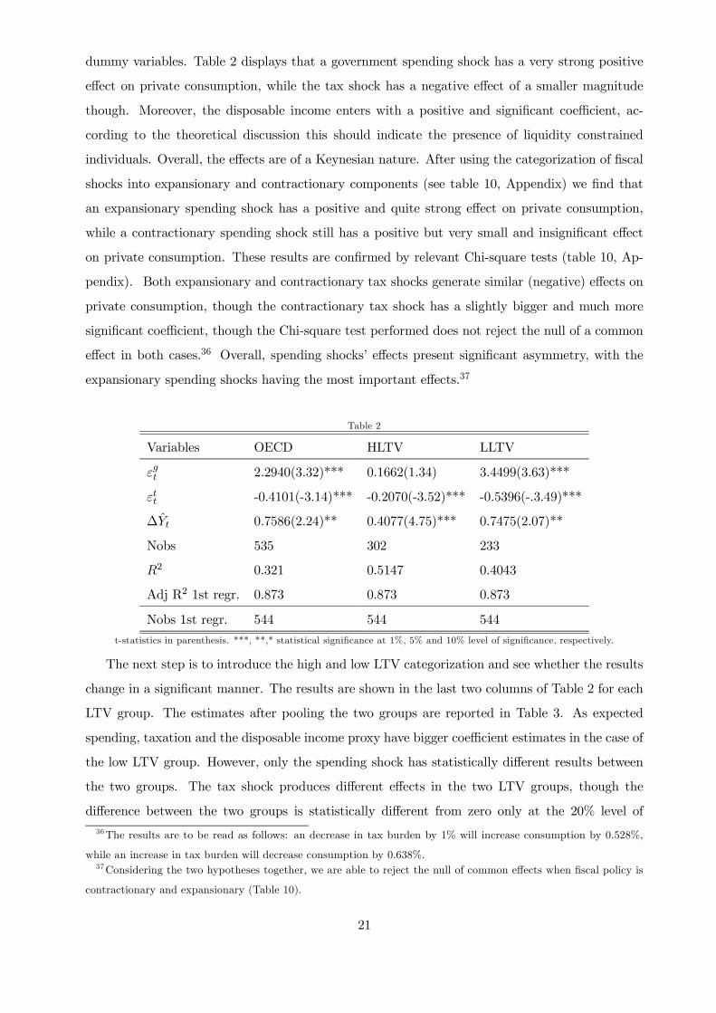
dummy variables. Table 2 displays that a government spending shock has a very strong positive

effect on private consumption, while the tax shock has a negative effect of a smaller magnitude

though. Moreover, the disposable income enters with a positive and significant coefficient, ac-

cording to the theoretical discussion this should indicate the presence of liquidity constrained

individuals. Overall, the effects are of a Keynesian nature. After using the categorization of fiscal

shocks into expansionary and contractionary components (see table 10, Appendix) we find that

an expansionary spending shock has a positive and quite strong effect on private consumption,

while a contractionary spending shock still has a positive but very small and insignificant effect

on private consumption. These results are confirmed by relevant Chi-square tests (table 10, Ap-

pendix). Both expansionary and contractionary tax shocks generate similar (negative) effects on

private consumption, though the contractionary tax shock has a slightly bigger and much more

significant coefficient, though the Chi-square test performed does not reject the null of a common

effect in both cases.36 Overall, spending shocks’ effects present significant asymmetry, with the

expansionary spending shocks having the most important effects.37

Table 2

Variables OECD

εgt 2.2940(3.32)***

εtt -0.4101(-3.14)***

∆Yt 0.7586(2.24)**

Nobs 535

R2 0.321

Adj R2 1st regr. 0.873

Nobs 1st regr. 544

HLTV LLTV

0.1662(1.34) 3.4499(3.63)***

-0.2070(-3.52)*** -0.5396(-.3.49)***

0.4077(4.75)*** 0.7475(2.07)**

302 233

0.5147 0.4043

0.873 0.873

544 544

t-statistics in parenthesis. ***, **,* statistical significance at 1%, 5% and 10% level of significance, respectively.

The next step is to introduce the high and low LTV categorization and see whether the results

change in a significant manner. The results are shown in the last two columns of Table 2 for each

LTV group. The estimates after pooling the two groups are reported in Table 3. As expected

spending, taxation and the disposable income proxy have bigger coefficient estimates in the case of

the low LTV group. However, only the spending shock has statistically different results between

the two groups. The tax shock produces different effects in the two LTV groups, though the

difference between the two groups is statistically different from zero only at the 20% level of36The results are to be read as follows: an decrease in tax burden by 1% will increase consumption by 0.528%,

while an increase in tax burden will decrease consumption by 0.638%.37Considering the two hypotheses together, we are able to reject the null of common effects when fiscal policy is

contractionary and expansionary (Table 10).

21

significance. Therefore, fiscal policy shocks and particularly government spending shocks have

asymmetric effects in the two LTV groups, suggesting that liquidity constraints are important.

Table 3

Variables

εgtLLTV 3.4863(3.44)***

εgt (HLTV − LLTV ) -3.3630(-3.30)***

εttLLTV -0.5264(-3.20)***

εtt(HLTV − LLTV ) 0.2431(1.34)

∆YtLLTV 0.7626(2.14)**

∆Yt(HLTV − LLTV ) -0.0837(-0.33)

Nobs 535

R2 0.3755

Nobs & R2 in the 1st regr. 544 (0.873)

t-statistics in parenthesis. ***, **,* statistical significance at 1%, 5% and 10% level of significance, respectively.

In the high LTV group (table 10, Appendix), contractionary and expansionary spending shocks

have a positive effect of a similar magnitude, but they are statistically insignificant. The expansion-

ary tax shock seems to have a much bigger impact on private consumption than the contractionary

tax shock, i.e. a decrease in taxation increases consumption by about the double of the absolute

value of a private consumption decrease following an increase in taxation. However, relevant

Chi-square tests do not confirm this result.

Both spending and tax shocks of expansionary and contractionary nature are of a bigger magni-

tude in the low-LTV group. Expansionary spending shocks have a much more pronounced, positive

and significant effect on private consumption, compared to contractionary spending shocks. While

it is contractionary tax shocks that appear to have a significant impact on consumption. Though,

the Chi-square tests reported support only the case of different spending effects and not tax effects.

Considering both hypotheses together we are able to reject the null of common effects when fiscal

policy is expansionary and contractionary. After pooling all observations (table 11, Appendix)

expansionary spending shocks in the low-LTV group are the driving force of the asymmetry be-

tween the effects of spending shocks in OECD countries (the expansionary spending shocks are

of a much bigger magnitude in the low-LTV group). In addition, there is significant asymmetry

in the effects of a contractionary tax shock between the two LTV groups, with the effect being

almost three times bigger in absolute value in the case of the low-LTV group. Hence, an increase

in spending and an increase in taxation are translated into much bigger consumption changes in

the low-LTV group, that is characterized by less developed consumer credit markets, than in the

22

high LTV group.

Before turning to examine the role of liquidity constraints in the transmission of fiscal shocks

in recessions and expansions, we analyze how tax and spending shocks affect private consumption

in recessions and expansions in all the nineteen OECD countries considered. The results will be

suggestive of the effectiveness of fiscal policy over the business cycle and will serve as a useful

benchmark in order to evaluate the effect that the interaction of the degree of development of

consumer credit markets (as described by the LTV ratio) with fiscal policy shocks has on private

consumption in upturns and downturns of economic activity.

We estimate two versions of the model. In the first one, according to our simple theoretical

framework, the proxy ∆Yt captures the effects of anticipated income changes on private consump-

tion of liquidity constrained individuals. While in the second ∆Yt is allowed to have a different

effect in Bad and Good times, i.e. allow for liquidity constraints to bind both in Good and Bad

times; we expect though the result to be stronger in Bad times. In both cases we include a full

set of country and year dummy variables. Tables 4 and 5 present the estimates that correspond

to the four definitions of Bad times.

When examining DY, we see that spending shocks have a positive effect on private consumption

which much more pronounced in Bad times. Tax shocks, have a negative effect in both states of

nature with their effect being stronger and more significant in Bad times. The disposable income

proxy has a bigger effect in economic recessions. Though, Chi-square tests indicate that only the

effect of the spending shock has statistically different effects in Good and Bad times.

After decomposing the fiscal shocks into expansionary and contractionary categories, in the

case of definition DY, we see (table 12 Appendix) that an expansionary spending shock generates

a bigger (positive) impact effect on private consumption than a contractionary spending shock

when in Bad times. So an increase in spending affects consumption (positively) by much more

than a corresponding decrease when in Bad times; this appears is not the case in Good times as

can be seen by the reported Chi-square tests. Moreover, there is a statistically significant and

much bigger (positive) effect on private consumption following an expansionary spending shock in

Bad than in Good times.

A contractionary tax shock in Bad times appears to affect consumption to a greater extent

than an expansionary tax shock in Bad times, though the Chi-square tests reported in Table 12.1

do not confirm this result. In Good times there is an indication of asymmetric effects, with bigger

coefficient (in absolute values) for the case of an expansionary tax shock, though the relevant test

performed does not reject the null of a common coefficient for expansionary and contractionary

tax shocks. While, contractionary tax shocks have a bigger (negative) and more significant impact

23

effect on private consumption in Bad times, than in Good times. Whereas, for expansionary tax

shocks we cannot reject the null of a common effect both in Bad and Good times.

TABLE 4

Variables DY DY

εgtBad 3.6949(3.62)*** 3.8225(3.82)***

εgtGood 0.7130(0.88) 0.3064(0.41)

εttBad -0.5711(-3.61)*** -0.6199(-3.90)***

εttGood -0.3422(-1.00) -0.2012(-0.62)

∆Yt 0.7467(2.27)** -

∆YtBad - 0.8351(2.48)**

∆YtGood - 0.6000(1.74)*

Nobs 535 535

NofBad Times 261 261

R2 0.368 0.386

X2(and p-values):bg=gg 5.22(0.0224) 7.88(0.0050)

X2 :bt=gt 0.36(0.5477) 1.32(0.2505)

X2 : b∆Yt = g∆Yt - 1.18(0.2779)

Adj.R2 & Nobs 1st regr. 0.873 (544)

t-statistics in parenthesis (in X2 tests we report p-values).*

**, **,* statistical significance at 1%, 5% and 10% level of signif., respectively.

24

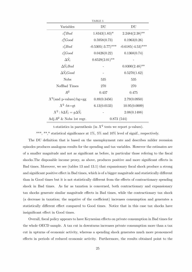
TABLE 5

Variables DU DU

εgtBad 1.8343(1.83)* 2.2484(2.38)**

εgtGood 0.5958(0.73) 0.1963(0.26)

εttBad -0.5305(-3.77)*** -0.6185(-4.53)***

εttGood 0.0426(0.22) 0.1368(0.74)

∆Yt 0.6529(2.01)** -

∆YtBad - 0.8300(2.48)**

∆YtGood - 0.5270(1.62)

Nobs 535 535

NofBad Times 270 270

R2 0.437 0.475

X2(and p-values):bg=gg 0.89(0.3456) 2.79(0.0950)

X2 :bt=gt 6.13(0.0133) 10.95(0.0009)

X2 : b∆Yt = g∆Yt - 2.08(0.1488)

Adj.R2 & Nobs 1st regr. 0.873 (544)

t-statistics in parenthesis (in X2 tests we report p-values).

***, **,* statistical significance at 1%, 5% and 10% level of signif., respectively.

The DU definition that is based on the unemployment rate and describes milder recession

episodes produces analogous results for the spending and tax variables. However the estimates are

of a smaller magnitude and not as significant as before, in particular those refering to the fiscal

shocks.The disposable income proxy, as above, produces positive and more significant effects in

Bad times. Moreover, we see (tables 13 and 13.1) that expansionary fiscal shock produce a strong

and significant positive effect in Bad times, which is of a bigger magnitude and statistically different

than in Good times but it is not statistically different from the effects of contractionary spending

shock in Bad times. As far as taxation is concerned, both contractionary and expansionary

tax shocks generate similar magnitude effects in Bad times, while the contractionary tax shock

(a decrease in taxation; the negative of the coefficient) increases consumption and generates a

statistically different effect compared to Good times. Notice that in this case tax shocks have

insignificant effect in Good times.

Overall, fiscal policy appears to have Keynesian effects on private consumption in Bad times for

the whole OECD sample. A tax cut in downturns increases private consumption more than a tax

cut in upturns of economic activity, whereas a spending shock generates much more pronounced

effects in periods of reduced economic activity. Furthermore, the results obtained point to the

25

following: Expansionary spending shocks in Bad times are more important in generating positive

effects in consumption and differ significantly both with respect to the corresponding effects in

Good times and the effects of a contractionary spending shock in Bad times. With respect to

taxation, expansionary tax shocks in Good times (a decrease in taxation, i.e. the negative of the

coefficient estimate) raise significantly consumption, mainly for DY (though the magnitude of the

effect does not differ significantly from the effect in consumption caused by a tax hike as part

of a contractionary tax policy in Good times); while a contractionary tax shock in Bad times

generates a significant reduction in private consumption, which is statistically different from the

corresponding effect in Good times, but not statistically different from the magnitude effect of a

expansionary tax shock (a tax cut) in Bad times.

Hence fiscal policy (particularly an expansionary spending shock) is more effective in mitigating

economic slumps rather than in muting booms, with respect to its effect on private consumption.

As far as taxation is concerned, we see that tax effects on consumption are stronger in Bad times

particularly because tax shocks, contractionary or expansionary, are equally important in Bad

times, while at the same time contractionary shocks in Bad times affect private consumption to a

greater extent relative to their corresponding effect in Good times. Alternatively we could say that

government spending is a more effective mechanism in shortening recession episodes than length-

ening expansions in OECD countries. Tax policy has very negative effects on private economic

activity if pursued in a contractionary manner in particular in Bad times than in Good times;

whereas there are no significant indications that its contractionary (tax hike) and expansionary

(tax cut) components produce asymmetric effects (in terms of the magnitude of the coefficient) in

Bad times.38

A possible justification for these results is the presence of liquidity constraints that bind for a

fraction of the population in all OECD countries during Bad times, so that unanticipated fiscal

policy actions that increase or decrease disposable income will induce them to consume more or

less, respectively.39 Next, we will evaluate the implications of credit constraints.

4.2.1.1 The effects of credit constraints in recessions and expansions In this section

we will examine the effects of consumer credit availability on the way that fiscal policy affects

38 In case of a tax hike consumption decreases, the opposite in case of a tax cut, but the result is of a symmetric

nature.39Alternatively, the fiscal policy shocks might be countercyclical, with their effect being inherently stronger in

recessions because. Though, even in that case liquidity constraints should bind, otherwise individuals should be able

to smooth their consumption.

26

consumption behavior. Consumer credit availability is determined by the LTV ratio40.

The results presented on Table 6 make use of the DY definition of Bad times and refer to

the high and low LTV groups. A government spending shock affects in a positive and significant

manner private consumption in Bad times with respect to the high LTV group; though in Good

times its effect is not statistically significant, and the coefficient has a negative sign. The tax

variable has a negative and significant effect which appears to be of a similar magnitude in both

Good and Bad times. The disposable income proxy enters with a positive and significant coefficient

both in Good and Bad times, though its effect is bigger in Good times.

Fiscal policy is more effective for the low LTV group. A government spending shock has a

much bigger and statistically significant coefficient in Bad times, on top of that the tax shocks

have a bigger effect and are statistically significant only in Bad times. The disposable income

proxy has a bigger effect on private consumption in the low LTV group, with its effect being

more pronounced, as expected, in Bad times. However, it is only the spending shock that appears

to have statistically different effects (at conventional levels of statistical significance) on private

consumption in Bad and Good times.

Therefore, spending shocks have more pronounced effects in Bad times for both LTV groups,

though the magnitude of the coefficients is much bigger when considering the low LTV group. Tax

shocks have a bigger coefficient for the low LTV group rather than the high LTV group, however,

in both cases we cannot reject the null of a similar effect in Good and Bad times. Analogously, the

effect of the disposable income proxy is bigger in the low LTV group. In addition, the disposable

income proxy has a stronger effect in Good times for the high LTV group, whereas its effect is

bigger in Bad times for the low LTV group (though only at the 20% percent level of significance).

40As before we estimate two versions of equation (22). The first one imposes a common ∆Yt in Good and

Bad times, while in the second ∆Yt is allowed to have a different effect in upturns and downturns. A full set of

country and year dummy variables have been included, and the estimation is conducted for a high and a low LTV

country-year groups. The Prais-Winsten estimation procedure that allows for panel-level heteroskedastic AR(1)

error structure was used. Qualitatively similar results were obtained when we estimated the model with pooled OLS

with Newey-West standards errors.

27

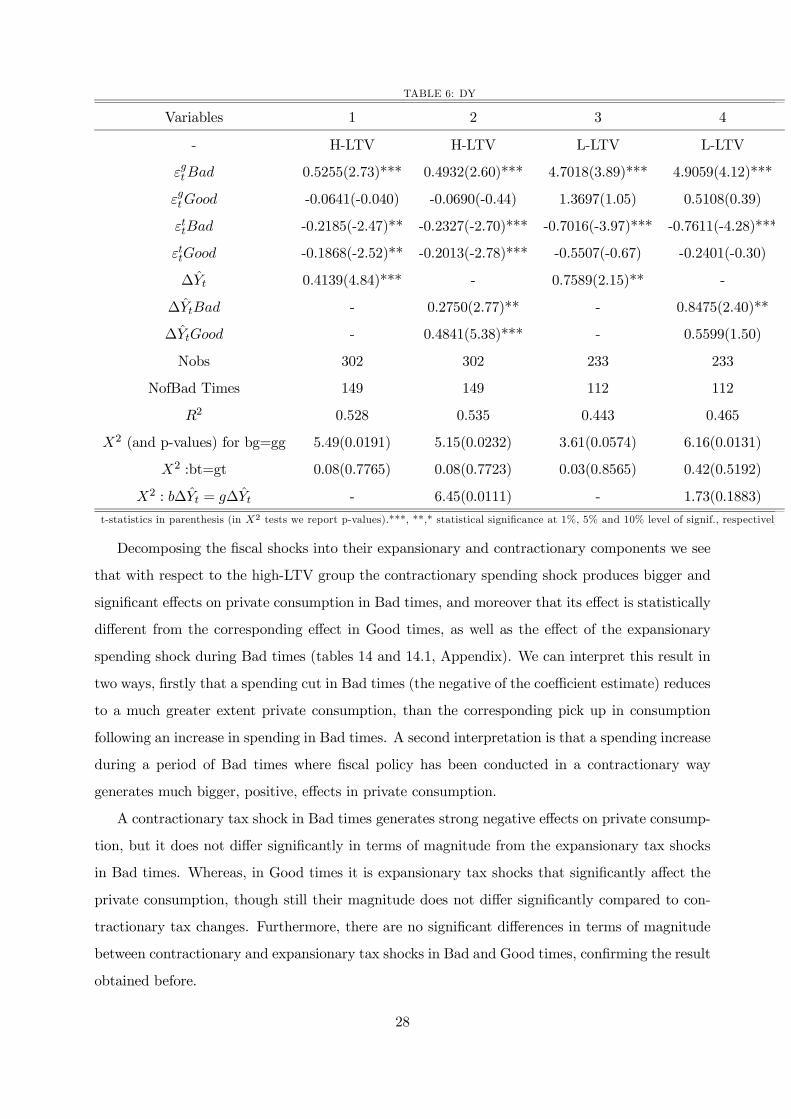
TABLE 6: DY

Variables 1 2 3 4

- H-LTV H-LTV L-LTV L-LTV

εgtBad 0.5255(2.73)*** 0.4932(2.60)*** 4.7018(3.89)*** 4.9059(4.12)***

εgtGood -0.0641(-0.040) -0.0690(-0.44) 1.3697(1.05) 0.5108(0.39)

εttBad -0.2185(-2.47)** -0.2327(-2.70)*** -0.7016(-3.97)*** -0.7611(-4.28)***

εttGood -0.1868(-2.52)** -0.2013(-2.78)*** -0.5507(-0.67) -0.2401(-0.30)

∆Yt 0.4139(4.84)*** - 0.7589(2.15)** -

∆YtBad - 0.2750(2.77)** - 0.8475(2.40)**

∆YtGood - 0.4841(5.38)*** - 0.5599(1.50)

Nobs 302 302 233 233

NofBad Times 149 149 112 112

R2 0.528 0.535 0.443 0.465

X2 (and p-values) for bg=gg 5.49(0.0191) 5.15(0.0232) 3.61(0.0574) 6.16(0.0131)

X2 :bt=gt 0.08(0.7765) 0.08(0.7723) 0.03(0.8565) 0.42(0.5192)

X2 : b∆Yt = g∆Yt - 6.45(0.0111) - 1.73(0.1883)

t-statistics in parenthesis (in X2 tests we report p-values).***, **,* statistical significance at 1%, 5% and 10% level of signif., respectively

Decomposing the fiscal shocks into their expansionary and contractionary components we see

that with respect to the high-LTV group the contractionary spending shock produces bigger and

significant effects on private consumption in Bad times, and moreover that its effect is statistically

different from the corresponding effect in Good times, as well as the effect of the expansionary

spending shock during Bad times (tables 14 and 14.1, Appendix). We can interpret this result in

two ways, firstly that a spending cut in Bad times (the negative of the coefficient estimate) reduces

to a much greater extent private consumption, than the corresponding pick up in consumption

following an increase in spending in Bad times. A second interpretation is that a spending increase

during a period of Bad times where fiscal policy has been conducted in a contractionary way

generates much bigger, positive, effects in private consumption.

A contractionary tax shock in Bad times generates strong negative effects on private consump-

tion, but it does not differ significantly in terms of magnitude from the expansionary tax shocks

in Bad times. Whereas, in Good times it is expansionary tax shocks that significantly affect the

private consumption, though still their magnitude does not differ significantly compared to con-

tractionary tax changes. Furthermore, there are no significant differences in terms of magnitude

between contractionary and expansionary tax shocks in Bad and Good times, confirming the result

obtained before.

28

Expansionary spending shocks in Bad times are the most important factor that affects private

consumption in the low-LTV group, and it is statistically different from contractionary spending

shocks in Bad times, and expansionary spending shocks in Good times. In addition, as for the high-

LTV group, contractionary tax shocks in Bad times affect in a significant manner consumption

changes, though its effect differs significantly from the corresponding effect of a expansionary tax

shock in Bad times. Hence, a tax hike in Bad times reduces consumption, but not more that the

corresponding increase in consumption following a tax cut in Bad times. Therefore, the bigger

source of asymmetry comes from the spending shocks, with the contractionary component being

more influential in the high LTV group and the expansionary component in the low-LTV group.

According to the DU definition of Bad times (table 7) that makes use of the cyclical component

of the unemployment rate, the effects of spending shocks on private consumption for the high LTV

group follow the same pattern as those under the first definition of Bad times, i.e. the coefficient

estimates are bigger and significant (only) in Bad times. Tax shocks appear to have a relatively

stronger effect in Good times, though this is not supported by relevant Chi-square tests. The

disposable income proxy has significant and positive coefficient estimates in both Good and Bad

times, moreover we cannot reject the null of a similar effect in both states of nature. When

examining the coefficient estimates for the low LTV group we see that spending shocks have much

bigger effects compared to high LTV group, in addition the effect in Bad times is more pronounced

compared to that in Good times. The tax shocks have coefficients of bigger magnitude compared

to the high LTV group in Bad times, with their effect being insignificantly estimated in Good

times. The disposable income proxy has a bigger effect on private consumption relative to the

high LTV group, having also a more pronounced effect during recessions as expected.

29

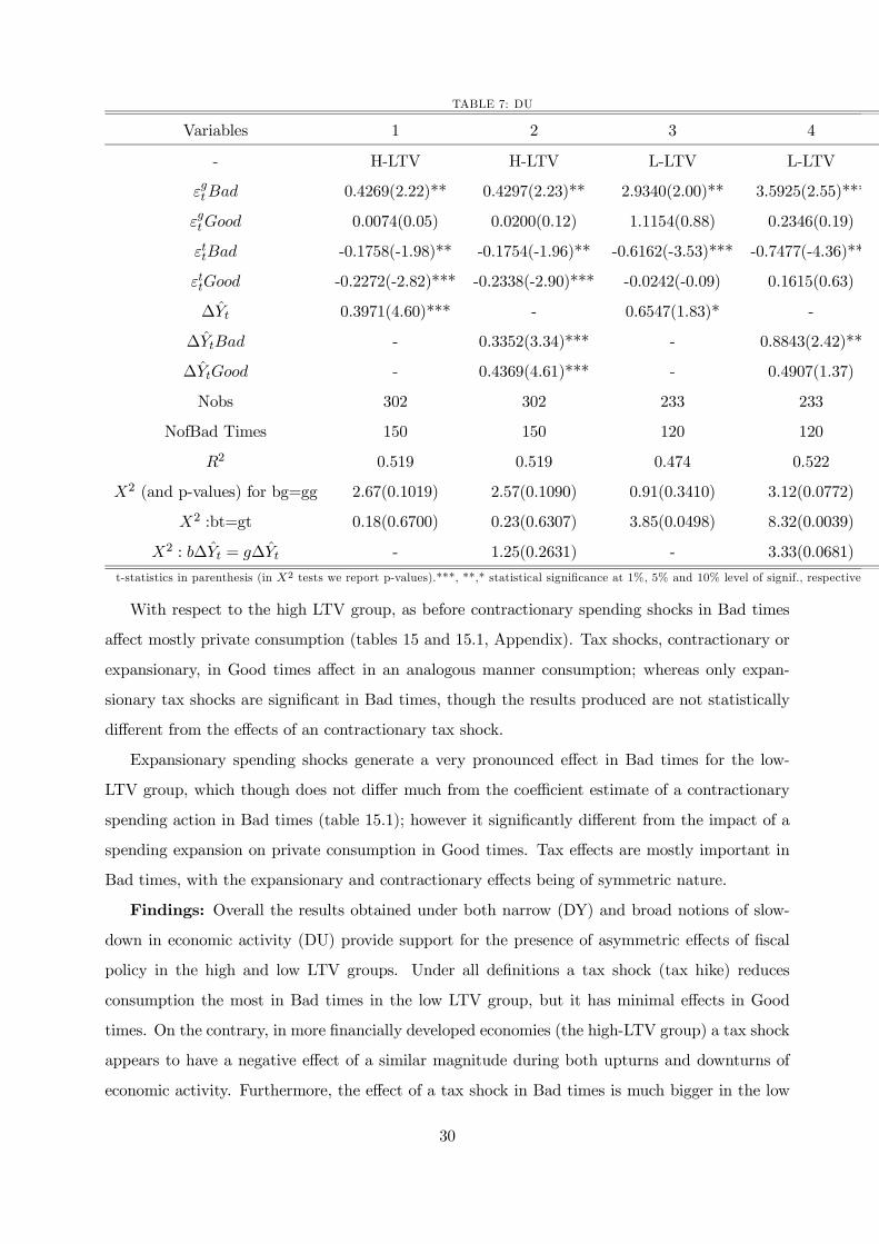
TABLE 7: DU

Variables 1 2 3 4

- H-LTV H-LTV L-LTV L-LTV

εgtBad 0.4269(2.22)** 0.4297(2.23)** 2.9340(2.00)** 3.5925(2.55)***

εgtGood 0.0074(0.05) 0.0200(0.12) 1.1154(0.88) 0.2346(0.19)

εttBad -0.1758(-1.98)** -0.1754(-1.96)** -0.6162(-3.53)*** -0.7477(-4.36)**

εttGood -0.2272(-2.82)*** -0.2338(-2.90)*** -0.0242(-0.09) 0.1615(0.63)

∆Yt 0.3971(4.60)*** - 0.6547(1.83)* -

∆YtBad - 0.3352(3.34)*** - 0.8843(2.42)**

∆YtGood - 0.4369(4.61)*** - 0.4907(1.37)

Nobs 302 302 233 233

NofBad Times 150 150 120 120

R2 0.519 0.519 0.474 0.522

X2 (and p-values) for bg=gg 2.67(0.1019) 2.57(0.1090) 0.91(0.3410) 3.12(0.0772)

X2 :bt=gt 0.18(0.6700) 0.23(0.6307) 3.85(0.0498) 8.32(0.0039)

X2 : b∆Yt = g∆Yt - 1.25(0.2631) - 3.33(0.0681)

t-statistics in parenthesis (in X2 tests we report p-values).***, **,* statistical significance at 1%, 5% and 10% level of signif., respectivel

With respect to the high LTV group, as before contractionary spending shocks in Bad times

affect mostly private consumption (tables 15 and 15.1, Appendix). Tax shocks, contractionary or

expansionary, in Good times affect in an analogous manner consumption; whereas only expan-

sionary tax shocks are significant in Bad times, though the results produced are not statistically

different from the effects of an contractionary tax shock.

Expansionary spending shocks generate a very pronounced effect in Bad times for the low-

LTV group, which though does not differ much from the coefficient estimate of a contractionary

spending action in Bad times (table 15.1); however it significantly different from the impact of a

spending expansion on private consumption in Good times. Tax effects are mostly important in

Bad times, with the expansionary and contractionary effects being of symmetric nature.

Findings: Overall the results obtained under both narrow (DY) and broad notions of slow-

down in economic activity (DU) provide support for the presence of asymmetric effects of fiscal

policy in the high and low LTV groups. Under all definitions a tax shock (tax hike) reduces

consumption the most in Bad times in the low LTV group, but it has minimal effects in Good

times. On the contrary, in more financially developed economies (the high-LTV group) a tax shock

appears to have a negative effect of a similar magnitude during both upturns and downturns of

economic activity. Furthermore, the effect of a tax shock in Bad times is much bigger in the low

30

LTV group as can judged from the magnitude of the coefficient estimates.

Moreover, after decomposing the tax shocks into their contractionary and expansionary com-

ponents we see that they are affecting consumption effectively both in Bad and Good times for the

high-LTV group. In particular the most pronounced effects on private consumption are obtained

when considering the following cases: a contractionary tax shock in Bad times as defined by DY

(i.e. a tax hike or a tax cut when tax policy was previously set in a contractionary manner), an

expansionary tax shock in Bad times as defined by DU (i.e. a tax cut) and an expansionary tax

shock in Good times.

In the low-LTV group the most pronounced effects on private consumption come from the

contractionary component of a tax shock. Hence, a tax cut in Bad times, when policy was

previously conducted in contractionary manner, boosts substantially private consumption (the

opposite if we consider a tax hike). The expansionary component of tax shocks is effective in Bad

times, though only in the case of less severe recession episodes (like DU).

Government spending shocks affect consumption expenditure the most during recessions in

both LTV groups, however the effect is much more pronounced in countries with less developed

financial systems as was predicted by the model. Additionally, in the high-LTV group it is the

contractionary component of spending shocks that affects consumption the most, i.e. a spending

cut during a recession period (e.g. in order to improve the fiscal balances) has devastating effects

on consumption; alternatively, a spending increase in a recession period, when fiscal policy was

pursued in an contractionary manner boosts effectively private consumption. On the other hand,

it is the expansionary component of spending shocks that raises private consumption in Bad times

for the low-LTV group, because an increase in government spending (in the presence of binding

liquidity constraints) raises disposable income encouraging people to increase their spending. The

disposable income proxy has positive and significant effects in both LTV groups, with its effect

being much more pronounced in the low LTV group as expected. In addition, there is limited

evidence that the coefficient estimates are of bigger magnitude in Bad times for the low LTV

group. On the contrary, when considering the high LTV group, in most cases, there is clear

evidence of a bigger coefficient in Good times.

Therefore, during recession episodes fiscal policy in the low LTV group shares (or drives)

the stabilization properties of the whole OECD sample case, i.e. fiscal policy (both spending

and tax) shocks are more effective in mitigating recessions rather than muting expansions, with

respect to its effect on private consumption. Alternatively, fiscal policy actions are more able

in shortening recessions than lengthening expansions. Whereas, for the high LTV group, an

unanticipated increase in spending boosts private expenditure only in Bad times as for the low

31

LTV group, however tax policy is equally effective under all states of nature. This is due to the

fact that taxation has a direct effect on individuals’ income and since most people can smooth

their consumption at all times, tax changes will have similar effects under all states of nature.

4.2.1.2 Robustness Test Nevertheless, the results obtained so far might be affected by the

fact that some or all the countries that have been categorized to the low-LTV group have switched

status from 1995 onwards, due to financial liberalization. According to Jappelli and Pagano (1994),

the LTV ratio was 60% in Austria, Japan and Portugal, 75% in Belgium and Netherlands, 50% in

Greece, and 56% in Italy in 1994. We shall explore how our results change if we assign Belgium

and Netherlands in the high LTV group from 1995 onwards. A similar exercise will be done for

the other two groups of countries i.e. Austria, Japan and Portugal, and finally Italy and Greece.

Under all definitions of Bad times the results remain qualitatively similar both for the high

and low LTV categories, the only difference is in quantitative terms. Specifically the coefficients

of all variables in most cases become bigger, in absolute terms, especially in Bad times for the

low LTV group, whereas for the high LTV group the coefficient estimates do not change much or

they decrease41. This implies that the effect of fiscal policy on private consumption is stronger in

recessions in the low LTV group, when fewer countries are characterized as having less financially

developed economies overtime. This is true only if OECD countries are converging in terms

of the development of their financial markets, and fewer countries or none is included in the

low LTV group after 19954243. Hence, in the event of convergence of financial development and

harmonization of financial systems in OECD countries overtime, all or most of the low LTV group

observations refer to the prior to 1995 period observations. In this case, fiscal policy (taxation and

government expenditure) in the low LTV group has greater impact on consumption especially in

Bad times, than if we allow the countries under consideration to be assigned to the low LTV group

after 1995. An explanation for this could be that fiscal policy has become less effective in boosting

41Results are available upon request.42When we assign Belgium and Netherland to the high LTV countries after 1995 the high LTV observations

increase from 302 to 316 and the low LTV observations decrease from 233 to 219. After including Japan, Portugal

and Austria in the high LTV group the observation becomes 337 and 198, respectively for the high and low LTV

countries. Finally, after including Greece and Italy in the high LTV group the observations used in the regressions

are 351 and 184 respectively for the high and low LTV groups.43With respect to DY, after the reassignment of Belgium and Netherlands to the high LTV group after 1995 we

have 154 and 107 Bad time episodes, respectively for the high and low LTV groups. When reassigning Austria,

Japan and Portugal we get 163 and 98 episodes of Bad times respectively in high and low LTV groups. After

reassigning Greece and Italy to the high LTV group after 1995 we get 169 and 92 episodes of bad times, respectively

in the two LTV groups. When considering DU we have 163 and 98, then 168 and 98 and finally 176 and 90 Bad

time episodes in high and low LTV groups.

32

output and private demand overtime in the event of financial liberalization and abolishment of

restrictions on credit availability to consumers44.

5 Conclusions

This paper has presented in a simple theoretical framework the idea that fiscal policy can have

asymmetric effects on consumption in recessions and expansions in the presence of binding liquidity

constraints. Fiscal policy will be more effective in stimulating private consumption and pushing the

economy out of a recession, when liquidity constraints bind for a large fraction of the population.

This idea was investigated empirically on a panel of nineteen OECD countries.

Before characterizing periods of expansions and recessions using alternative definitions, we

showed that, in OECD countries, fiscal policy has Keynesian effects on private consumption ex-

penditure, i.e. a spending shock has a positive effect and a tax shock has a negative effect on

private consumption, with the spending effect being more pronounced. Moreover, it is the ex-

pansionary component of the spending shocks (or expansionary spending shocks) that exert the

bigger effect on private consumption rather than their contractionary component (or contactionary

spending shocks); whereas the contractionary and expansionary components of the tax shocks af-

fect symmetrically private consumption. After considering recession and expansion episodes, we

found that both tax and spending shocks affect consumption changes in Bad times more than in

Good times. This happens because private consumption is affected the most by the expansion-

ary component of spending shocks in Bad times, while both contractionary and expansionary tax

shocks are important in Bad times.

Following Jappelli and Pagano (1994), we used as a proxy for credit constraints the maximum

ratio of the loan to the value of the house in housing mortgages (LTV ratio), and we assigned

country-decade observations to a high and low LTV group following the work of Perotti (1999).

Using this measure we showed that fiscal policy has asymmetric effects in high and low LTV groups.

Specifically, a spending shock has much more pronounced effects in the low LTV group than in the

high LTV group (in particular, the expansionary component of a spending shock), similarly for the

tax shock, though the results appear to be less significant (in this case the difference is statistically

significant when considering the effects of the contractionary component of a tax shock).

After introducing in the analysis the alternative recession and expansion categorizations we

found that the results provide evidence for the presence of asymmetric effects of fiscal policy in

upturns and downturns in countries with more and less developed consumer credit markets. In

44Perotti (2004) examined the fiscal multiplier in the US, UK, Germany, Australia, and New Zealand and discussed

the possibility of declined potency of fiscal policy after the 1980.

33

most cases considered, tax shocks reduce consumption the most in Bad times when analyzing the

low LTV group (for the most severe recession episodes (as modeled by DY) this is attributed to the

contractionary component of the tax shock, i.e. a tax cut in Bad times, if policy was previously

conducted in contractionary manner, boosts significantly private consumption (whereas a tax hike

decreases consumption). When considering the high LTV group tax shocks have negative effects

of a similar magnitude during Good and Bad times (in particular we refer to the contractionary

component of tax shocks in Bad times (i.e. a tax hike or a tax cut when tax policy was previously

set in a contractionary manner) and the expansionary component of tax shocks in Good times

(i.e. a tax cut) when considering severe recession episodes (as those modeled by definition DY)).

Moreover, the effect of a tax shock in Bad times is much bigger in the low LTV group.

Government spending shocks affect private consumption expenditure the most during reces-

sions in both LTV groups, nevertheless the effect is much stronger in countries with less developed

financial systems as was anticipated. Though this effect originates from different components of

the spending shock in the two groups. For example, with respect to the high-LTV group it is the

contractionary component of the spending shocks that affects consumption the most45, while in the

low LTV group it is the expansionary component of government spending shocks that influences

private consumption the most. These hold both for narrow (DY) and broad (DU) definitions of

recession episodes, and can be explained by the fact that credit constraints bind for more people

in economies with less developed consumer credit markets, as well as, by the fact that during deep

recession episodes credit constraints bind for a larger fraction of the population, both in more and

less developed consumer credit markets.

The normative aspect of this analysis points to the need for discretionary fiscal policy actions

as a way of mitigating economic slumps. The unanticipated components of both tax policy and

government spending decisions are effective in Bad times in all OECD countries no matter what

the level of their financial development is, however their effects are much bigger in countries where

consumers have limited access to credit markets. In addition, when fiscal policy shocks are pro-

cyclical (i.e. negative spending shocks and positive tax shocks in recessions) then a “switch” to

countercyclical shocks (spending increases and tax cuts) could improve significantly consumption

outcomes. Hence, unless OECD countries (and specifically EMU countries) are converging over-

time in the degree of development of their financial systems there are reasons for not impairing

fiscal flexibility by stringent fiscal rules (such as the Stability and Growth Pact or SGP). Because,

for example, if countries are in a recession but still face the danger of breaching the 3 % limit

45Therefore a spending cut during a recession period has devastating effects on private consumption; alternatively,

a spending increase in a recession period, when fiscal policy was previously pursued in an contractionary manner,

boosts effectively private consumption.

34

implied by the SGP they will have to take one-off measures to correct their fiscal position, though

this will bring them into deeper recession since it will affect negatively private consumption.

6 References

Alesina, A. and Perotti, R., (1995). “Fiscal expansions and fiscal adjustments in OECD

countries,” Economic Policy, 21, 205-48.

Alesina, A. and Perotti, R., (1997). “Fiscal adjustments in OECD countries: Composition

and macroeconomic effects,” IMF Staff Papers, 210-48.

Alesina,A., Perotti, R., Schiantarelli, F. and Ardgana, S., (2002). “Fiscal Policy,

profits and investment,” American Economic Review, 92 (3), 571-89.

Attanasio, O. (1999). “Consumption,” in Handbook of Macroeconomics, Volume 1. Edited

by J.B. Taylor and M. Woodford, Elsevier Science, B.V.

Barsky, R.B., Mankiw, N.G. and Zeldes, S.P., (1986). “Ricardian consumers with

Keynesian propensities,” American Economic Review, 76, (4), 676-91.

Blanchard, O. (1993). “Suggestions for a new set of fiscal indicators,” in The Political econ-

omy of government debt, Harrie A. A. Vernon and Frans A. A.M. Van Winden, eds. (Amsterdam:

North-Holland).

Blanchard, O. and Perotti, R., (2002). “An empirical characterization of the dynamic

effects of changes in government spending and taxes on output,” Quarterly Journal of Economics,

117 (4), 1329-68.

Burnside, C. Eichenbaum, M. and Fisher, J.D.M., (2003). “Fiscal shocks and their

consequence” NBER, Working Paper 9772.

Fatas, A. and Mihov, I., (2001). “The effects of fiscal policy on consumption and employ-

ment: Theory and evidence,” CEPR, Discussion Paper 2760.

Gali, J., Lopez-Salido, J.D. and Valles, J., (2004). “Understanding the effects of gov-

ernment spending on consumption,” International Finance Discussion Papers, No.805, Board of

Governors of the Federal Reserve Bank.

Gavin, M. and Perotti,R., (1997), “Fiscal policy in Latin America”, NBERMacroeconomics

Annual, 11-61.

Giavazzi, F., Jappelli T. and Pagano, M., (2000). “Searching for non-linear effects of

fiscal policy: evidence from industrial and developing countries,” European Economic Review, 44,

1259-89.

Giavazzi, F. and Pagano, M., (1990). “Can severe fiscal contractions be expansionary?

Tales of two small European economies,” NBER Macroeconomics Annual, 75-116.

35

Giavazzi, F. and Pagano, M., (1996). “Non-keynesian effects of fiscal policy changes:

International evidence and the Swedish experience,” Swedish Economic Policy Review, 3, 67-103.

Giorgio, C., Richardson, P., Roseveare, D., and van den Noord, P. (1995). “Potential

output, output gaps, and structural budget balances”, OECD Economic Studies, 24, 167-209.

Jappelli, T. and Pagano, M., (1994). “Saving, growth, and liquidity constraints,”Quarterly

Journal of Economics, 109, 83-109

Lane, P.R., (2003). “The cyclical behaviour of fiscal policy: evidence from the OECD”,

Journal of Public Economics, 87, 2661-2675.

Lane, P.R. and Perotti, R., (2003). “The importance of composition of fiscal policy:

evidence from different exchange rate regimes”, Journal of Public Economics, 87, 2253-2279.

Mountford, A. and Uhlig, H., (2002). “What are the effects of fiscal policy shocks?”

CEPR, Discussion Paper 3338.

van den Noord, P. (2002). “Automatic stabilizers in the 1990s and the beyond”, in: M. Buti,

J. von Hagen, and C. Martinez-Mongay, eds: The behavior of fiscal authorities, 130-48, Palgrave,

New York.

OECD, (2003). “Economic Outlook, Sources and Methods”.

Perotti, R., (1999). “Fiscal policy in good times and bad,” Quarterly Journal of Economics,

114, (4), 1399-1436.

Perotti, R., (2004). “Estimating the effects of fiscal policy in OECD countries,” mimeo

IGIER - Universita’ Bocconi.

Perotti, R. and Kontopoulos, Y., (2002). “Fragmented fiscal policy”, Journal of Public

Economics, 86, 191-222.

Sorensen, B.E. and Yosha, O., (2001). “Is state fiscal policy asymmetric over the business

cycle?” Economic Review, Federal Reserve Bank of Kansas City.

World Bank, (2003), “World development indicators”, World Bank.

36

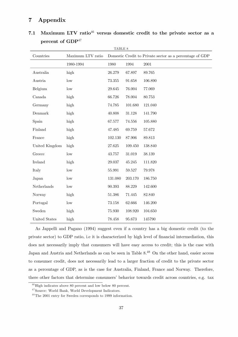
7 Appendix

7.1 Maximum LTV ratio46 versus domestic credit to the private sector as a

percent of GDP47

TABLE 8

Countries Maximum LTV ratio Domestic Credit to Private sector as a percentage of GDP

1980-1994 1980 1994 2001

Australia high 26.279 67.897 89.765

Austria low 73.355 91.658 106.890

Belgium low 29.645 76.004 77.069

Canada high 66.726 78.004 80.753

Germany high 74.785 101.680 121.040

Denmark high 40.808 31.128 141.790

Spain high 67.577 74.556 105.880

Finland high 47.485 69.759 57.672

France high 102.130 87.906 89.813

United Kingdom high 27.625 109.450 138.840

Greece low 43.757 31.019 38.139

Ireland high 29.037 45.245 111.820

Italy low 55.991 59.527 79.978

Japan low 131.080 203.170 186.750

Netherlands low 90.393 88.229 142.600

Norway high 51.386 71.445 82.840

Portugal low 73.158 62.666 146.200

Sweden high 75.930 108.920 104.650

United States high 78.458 95.673 145790

As Jappelli and Pagano (1994) suggest even if a country has a big domestic credit (to the

private sector) to GDP ratio, i.e it is characterized by high level of financial intermediation, this

does not necessarily imply that consumers will have easy access to credit; this is the case with

Japan and Austria and Netherlands as can be seen in Table 8.48 On the other hand, easier access

to consumer credit, does not necessarily lead to a larger fraction of credit to the private sector

as a percentage of GDP, as is the case for Australia, Finland, France and Norway. Therefore,

there other factors that determine consumers’ behavior towards credit across countries, e.g. tax

46High indicates above 80 percent and low below 80 percent.47Source: World Bank, World Development Indicators.48The 2001 entry for Sweden corresponds to 1999 information.

37

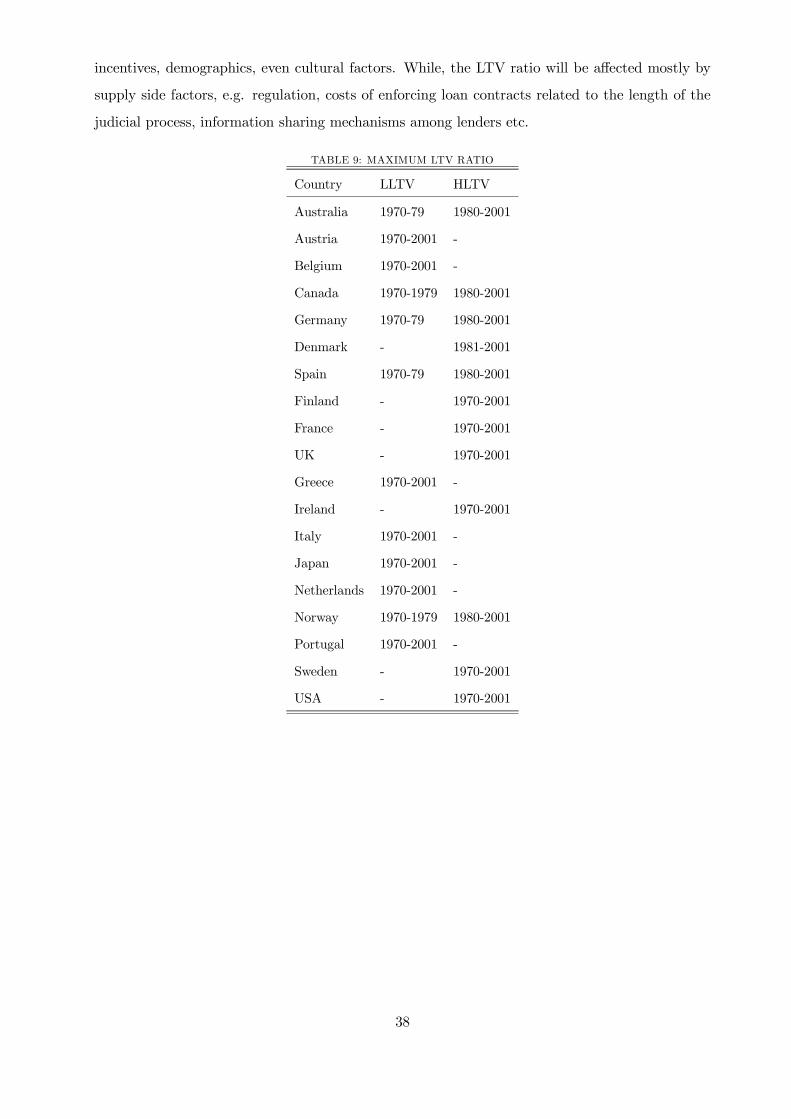
incentives, demographics, even cultural factors. While, the LTV ratio will be affected mostly by

supply side factors, e.g. regulation, costs of enforcing loan contracts related to the length of the

judicial process, information sharing mechanisms among lenders etc.

TABLE 9: MAXIMUM LTV RATIO

Country LLTV HLTV

Australia 1970-79 1980-2001

Austria 1970-2001 -

Belgium 1970-2001 -

Canada 1970-1979 1980-2001

Germany 1970-79 1980-2001

Denmark - 1981-2001

Spain 1970-79 1980-2001

Finland - 1970-2001

France - 1970-2001

UK - 1970-2001

Greece 1970-2001 -

Ireland - 1970-2001

Italy 1970-2001 -

Japan 1970-2001 -

Netherlands 1970-2001 -

Norway 1970-1979 1980-2001

Portugal 1970-2001 -

Sweden - 1970-2001

USA - 1970-2001

38

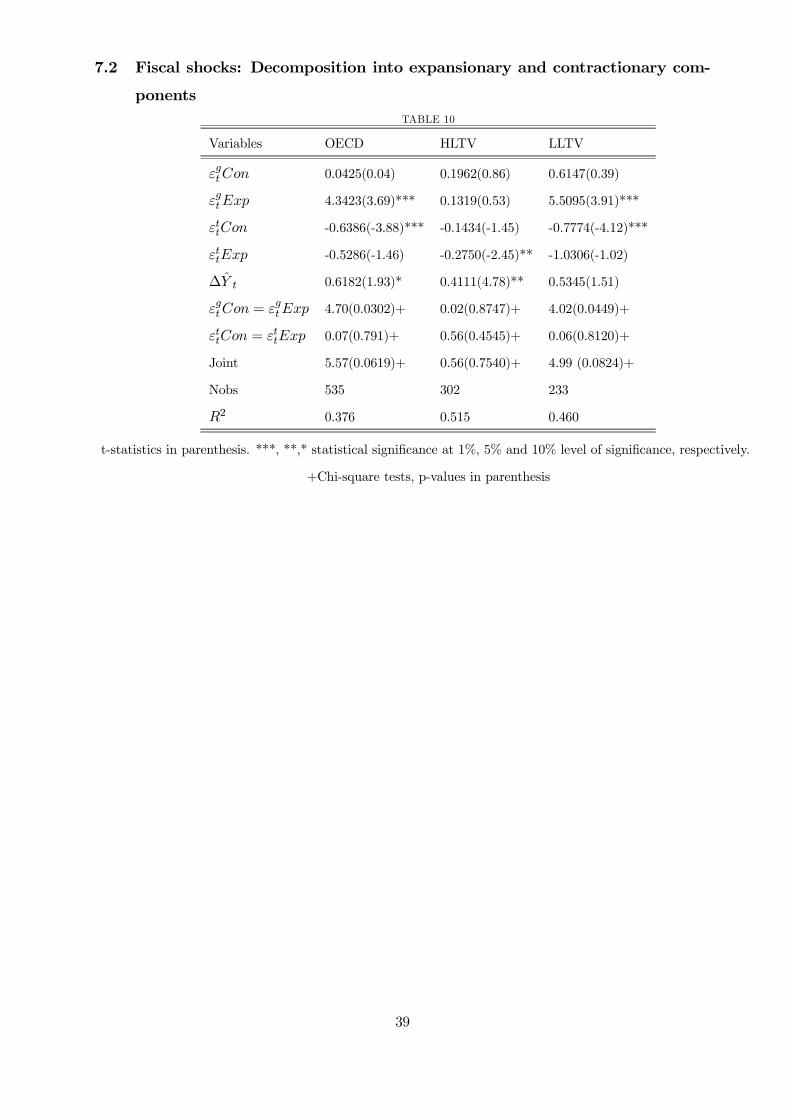
7.2 Fiscal shocks: Decomposition into expansionary and contractionary com-

ponentsTABLE 10

Variables OECD HLTV LLTV

εgtCon 0.0425(0.04) 0.1962(0.86) 0.6147(0.39)

εgtExp 4.3423(3.69)*** 0.1319(0.53) 5.5095(3.91)***

εttCon -0.6386(-3.88)*** -0.1434(-1.45) -0.7774(-4.12)***

εttExp -0.5286(-1.46) -0.2750(-2.45)** -1.0306(-1.02)

∆Y t 0.6182(1.93)* 0.4111(4.78)** 0.5345(1.51)

εgtCon = εgtExp 4.70(0.0302)+ 0.02(0.8747)+ 4.02(0.0449)+

εttCon = εttExp 0.07(0.791)+ 0.56(0.4545)+ 0.06(0.8120)+

Joint 5.57(0.0619)+ 0.56(0.7540)+ 4.99 (0.0824)+

Nobs 535 302 233

R2 0.376 0.515 0.460

t-statistics in parenthesis. ***, **,* statistical significance at 1%, 5% and 10% level of significance, respectively.

+Chi-square tests, p-values in parenthesis

39

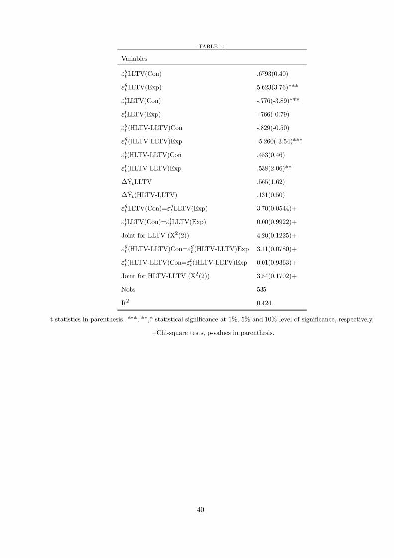
TABLE 11

Variables

εgtLLTV(Con) .6793(0.40)

εgtLLTV(Exp) 5.623(3.76)***

εttLLTV(Con) -.776(-3.89)***

εttLLTV(Exp) -.766(-0.79)

εgt (HLTV-LLTV)Con -.829(-0.50)

εgt (HLTV-LLTV)Exp -5.260(-3.54)***

εtt(HLTV-LLTV)Con .453(0.46)

εtt(HLTV-LLTV)Exp .538(2.06)**

∆YtLLTV .565(1.62)

∆Yt(HLTV-LLTV) .131(0.50)

εgtLLTV(Con)=εgtLLTV(Exp) 3.70(0.0544)+

εttLLTV(Con)=εttLLTV(Exp) 0.00(0.9922)+

Joint for LLTV (X2(2)) 4.20(0.1225)+

εgt (HLTV-LLTV)Con=εgt (HLTV-LLTV)Exp 3.11(0.0780)+

εtt(HLTV-LLTV)Con=εtt(HLTV-LLTV)Exp 0.01(0.9363)+

Joint for HLTV-LLTV (X2(2)) 3.54(0.1702)+

Nobs 535

R2 0.424

t-statistics in parenthesis. ***, **,* statistical significance at 1%, 5% and 10% level of significance, respectively,

+Chi-square tests, p-values in parenthesis.

40

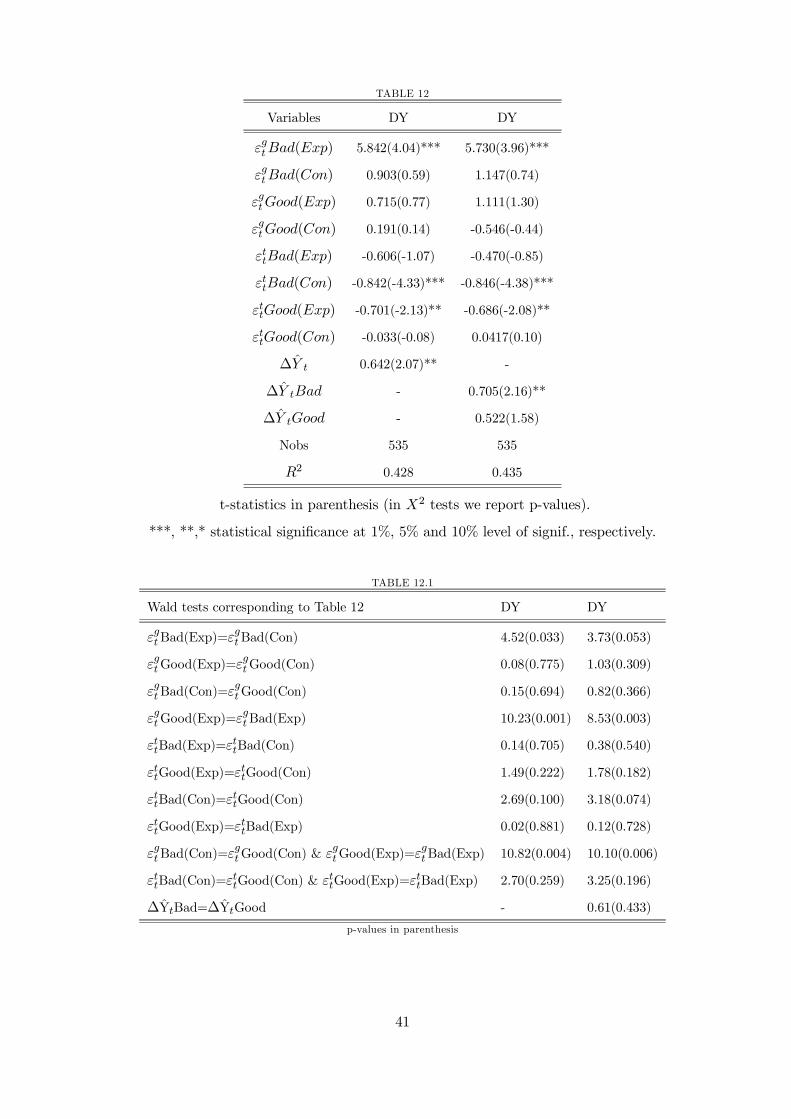
TABLE 12

Variables DY DY

εgtBad(Exp) 5.842(4.04)*** 5.730(3.96)***

εgtBad(Con) 0.903(0.59) 1.147(0.74)

εgtGood(Exp) 0.715(0.77) 1.111(1.30)

εgtGood(Con) 0.191(0.14) -0.546(-0.44)

εttBad(Exp) -0.606(-1.07) -0.470(-0.85)

εttBad(Con) -0.842(-4.33)*** -0.846(-4.38)***

εttGood(Exp) -0.701(-2.13)** -0.686(-2.08)**

εttGood(Con) -0.033(-0.08) 0.0417(0.10)

∆Y t 0.642(2.07)** -

∆Y tBad - 0.705(2.16)**

∆Y tGood - 0.522(1.58)

Nobs 535 535

R2 0.428 0.435

t-statistics in parenthesis (in X2 tests we report p-values).

***, **,* statistical significance at 1%, 5% and 10% level of signif., respectively.

TABLE 12.1

Wald tests corresponding to Table 12 DY DY

εgtBad(Exp)=εgtBad(Con) 4.52(0.033) 3.73(0.053)

εgtGood(Exp)=εgtGood(Con) 0.08(0.775) 1.03(0.309)

εgtBad(Con)=εgtGood(Con) 0.15(0.694) 0.82(0.366)

εgtGood(Exp)=εgtBad(Exp) 10.23(0.001) 8.53(0.003)

εttBad(Exp)=εttBad(Con) 0.14(0.705) 0.38(0.540)

εttGood(Exp)=εttGood(Con) 1.49(0.222) 1.78(0.182)

εttBad(Con)=εttGood(Con) 2.69(0.100) 3.18(0.074)

εttGood(Exp)=εttBad(Exp) 0.02(0.881) 0.12(0.728)

εgtBad(Con)=εgtGood(Con) & εgtGood(Exp)=ε

gtBad(Exp) 10.82(0.004) 10.10(0.006)

εttBad(Con)=εttGood(Con) & εttGood(Exp)=ε

ttBad(Exp) 2.70(0.259) 3.25(0.196)

∆YtBad=∆YtGood - 0.61(0.433)

p-values in parenthesis

41

TABLE 13

Variables DU DU

εgtBad(Exp) 4.207(2.49)** 3.882(2.34)**

εgtBad(Con) 1.031(0.70) 1.610(1.09)

εgtGood(Exp) 0.303(0.27) 0.987(1.02)

εgtGood(Con) 0.587(0.41) -0.508(-0.38)

εttBad(Exp) -1.010(-2.89)*** -0.839(-2.50)**

εttBad(Con) -0.731(-3.93)*** -0.743(-4.11)***

εttGood(Exp) -0.365(-0.65) -0.445(-0.84)

εttGood(Con) 0.130(0.59) 0.051(0.26)

∆Y t 0.642(2.06)** -

∆Y tBad - 0.792(2.41)**

∆Y tGood - 0.470(1.46)

Nobs 535 535

R2 0.449 0.475

t-statistics in parenthesis (in X2 tests we report p-values).

***, **,* statistical significance at 1%, 5% and 10% level of signif., respectively.

TABLE 13.1

Wald tests corresponding to Table 13 DU DU

εgtBad(Exp)=εgtBad(Con) 1.49(0.222) 0.76(0.383)

εgtGood(Exp)=εgtGood(Con) 0.02(0.891) 0.68(0.409)

εgtBad(Con)=εgtGood(Con) 0.06(0.809) 1.31(0.252)

εgtGood(Exp)=εgtBad(Exp) 4.61(0.031) 2.78(0.095)

εttBad(Exp)=εttBad(Con) 0.41(0.521) 0.05(0.819)

εttGood(Exp)=εttGood(Con) 0.59(0.442) 0.65(0.420)

εttBad(Con)=εttGood(Con) 9.87(0.001) 9.62(0.001)

εttGood(Exp)=εttBad(Exp) 0.88(0.347) 0.39(0.534)

εgtBad(Con)=εgtGood(Con) & εgtGood(Exp)=ε

gtBad(Exp) 4.98(0.083) 4.79(0.091)

εttBad(Con)=εttGood(Con) & εttGood(Exp)=ε

ttBad(Exp) 12.98(0.001) 12.63(0.001)

∆YtBad=∆YtGood - 1.89(0.169)

p-values in parenthesis

42

TABLE 14: DY

Variables 1 2 3 4

- H-LTV H-LTV L-LTV L-LTV

εgtBad(Exp) 0.040(0.12) 0.092(0.28) 6.746(4.32)*** 6.646(4.27)***

εgtBad(Con) 0.954(2.87)*** 0.890(2.62)*** 2.221(1.17) 2.402(1.25)

εgtGood(Exp) 0.002(0.01) -0.036(-0.12) 1.049(0.62) 1.917(1.13)

εgtGood(Con) -0.118(-0.46) -0.087(-0.34) 0.165(0.08) -1.301(-0.51)

εttBad(Exp) -0.091(-0.58) -0.105(-0.66) -2.343(-1.32) -1.914(-1.06)

εttBad(Con) -0.342(-2.33)** -0.335(-2.27)** -0.951(-4.57)*** -0.952(-4.59)***

εttGood(Exp) -0.317(-2.37)** -0.317(-2.38)** -0.765(-1.01) -0.897(-1.25)

εttGood(Con) -0.088(-0.81) -0.097(-0.88) -0.244(-0.22) -0.159(-0.14)

∆Y t 0.383(4.44)*** - 0.536(1.53) -

∆Y tBad - 0.342(3.38)*** - 0.604(1.67)*

∆Y tGood - 0.406(4.22)*** - 0.371(0.97)

Nobs 302 302 233 233

R2 0.545 0.543 0.512 0.517

t-statistics in parenthesis (in X2 tests we report p-values).***, **,* statistical significance at 1%, 5% and 10% level of signif., respectively

TABLE 14.1:DY

Wald tests corresponding to Table 14 HLTV HLTV LLTV LLTV

εgtBad(Exp)=εgtBad(Con) 2.83(0.092) 2.05(0.152) 2.92(0.087) 2.53(0.111)

εgtGood(Exp)=εgtGood(Con) 0.07(0.796) 0.01(0.915) 0.07(0.789) 0.76(0.382)

εgtBad(Con)=εgtGood(Con) 7.69(0.005) 5.95(0.014) 0.58(0.445) 1.39(0.238)

εgtGood(Exp)=εgtBad(Exp) 0.01(0.926) 0.09(0.762) 6.23(0.012) 4.20(0.040)

εttBad(Exp)=εttBad(Con) 0.98(0.322) 0.80(0.371) 0.58(0.446) 0.27(0.605)

εttGood(Exp)=εttGood(Con) 1.33(0.249) 1.22(0.269) 0.14(0.707) 0.28(0.595)

εttBad(Con)=εttGood(Con) 2.36(0.124) 2.01(0.156) 0.40(0.526) 0.49(0.483)

εttGood(Exp)=εttBad(Exp) 1.40(0.237) 1.20(0.273) 0.68(0.408) 0.29(0.592)

εgtBad(Con)=εgtGood(Con) & εgtGood(Exp)=ε

gtBad(Exp) 8.27(0.016) 7.03(0.029) 8.32(0.015) 8.15(0.017)

εttBad(Con)=εttGood(Con) & εttGood(Exp)=ε

ttBad(Exp) 2.95(0.228) 2.48(0.289) 1.10(0.578) 0.83(0.658)

∆YtBad=∆YtGood - 0.44(0.509) - 0.73(0.393)

p-values in parenthesis

43

TABLE 15: DU

Variables 1 2 3 4

- H-LTV H-LTV L-LTV L-LTV

εgtBad(Exp) 0.215(0.60) 0.306(0.86) 7.742(2.75)*** 7.184(2.63)***

εgtBad(Con) 0.676(2.06)** 0.601(1.84)* 2.686(1.47) 3.218(1.76)*

εgtGood(Exp) 0.066(0.22) 0.024(0.08) -0.372(-0.16) 1.614(0.72)

εgtGood(Con) -0.058(-0.21) -0.004(-0.02) 1.426(0.66) -1.002(-0.42)

εttBad(Exp) -0.329(-2.16)** -0.365(-2.33)** -2.721(-2.64)*** -2.458(-2.46)**

εttBad(Con) -0.004(-0.02) 0.040(0.24) -1.039(-3.67)*** -1.027(-3.75)***

εttGood(Exp) -0.273(-1.74)* -0.250(-1.58) -0.316(-0.25) -1.011(-0.89)

εttGood(Con) -0.185(-1.60) -0.211(-1.80)* 0.273(0.65) -0.003(-0.01)

∆Y t 0.409(4.72)*** - 0.609(1.84)* -

∆Y tBad - 0.325(3.19)*** - 0.733(2.15)**

∆Y tGood - 0.460(4.54)*** - 0.340(0.97)

Nobs 302 302 233 233

R2 0.522 0.518 0.520 0.542

t-statistics in parenthesis (in X2 tests we report p-values).***, **,* statistical significance at 1%, 5% and 10% level of signif., respectively

TABLE 15.1:DU

Wald tests corresponding to Table 15 HLTV HLTV LLTV LLTV

εgtBad(Exp)=εgtBad(Con) 0.66(0.416) 0.27(0.601) 1.80(0.179) 1.15(0.284)

εgtGood(Exp)=εgtGood(Con) 0.07(0.794) 0.00(0.952) 0.21(0.645) 0.43(0.512)

εgtBad(Con)=εgtGood(Con) 3.44(0.063) 2.33(0.126) 0.24(0.621) 1.98(0.159)

εgtGood(Exp)=εgtBad(Exp) 0.12(0.728) 0.42(0.516) 4.89(0.027) 2.47(0.115)

εttBad(Exp)=εttBad(Con) 1.50(0.221) 2.16(0.142) 2.15(0.142) 1.65(0.198)

εttGood(Exp)=εttGood(Con) 0.16(0.692) 0.03(0.861) 0.17(0.684) 0.56(0.455)

εttBad(Con)=εttGood(Con) 0.91(0.340) 1.61(0.204) 6.46(0.011) 4.41(0.035)

εttGood(Exp)=εttBad(Exp) 0.07(0.787) 0.29(0.591) 2.36(0.124) 1.03(0.309)

εgtBad(Con)=εgtGood(Con) & εgtGood(Exp)=ε

gtBad(Exp) 4.06(0.131) 3.48(0.175) 6.53(0.038) 7.01(0.030)

εttBad(Con)=εttGood(Con) & εttGood(Exp)=ε

ttBad(Exp) 0.91(0.634) 1.63(0.441) 12.08(0.002) 8.88(0.011)

∆YtBad=∆YtGood - 1.61(0.204) - 2.42(0.119)

p-values in parenthesis

44