constant-coefficient systems(1)
TRANSCRIPT
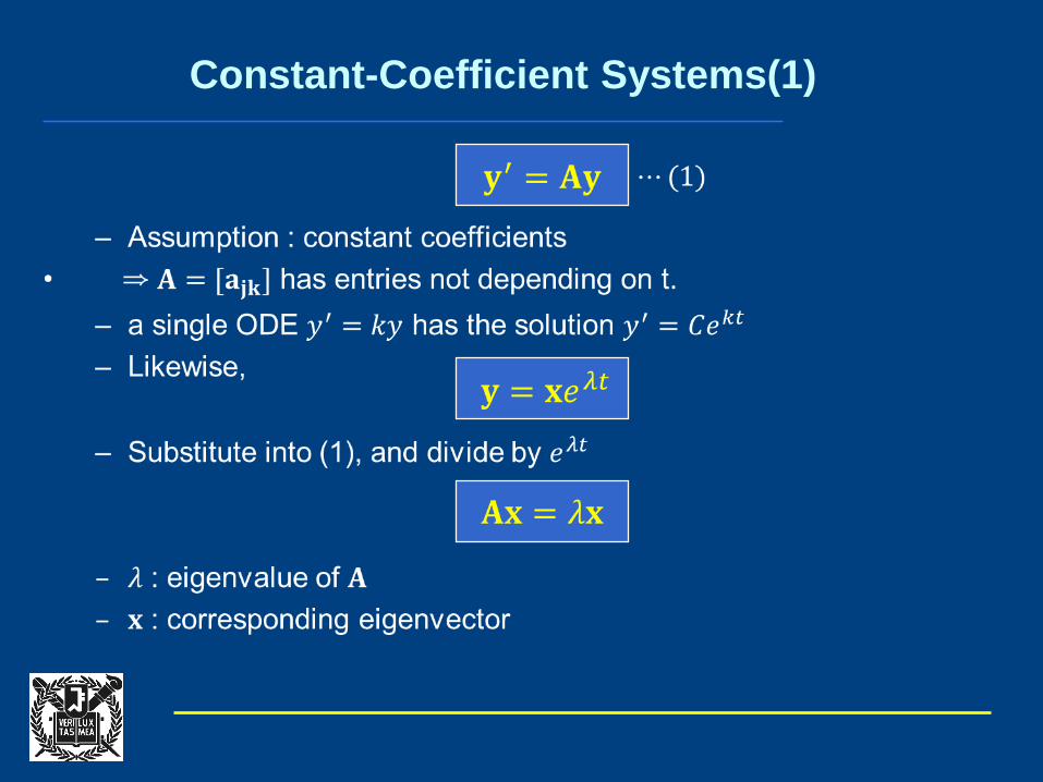
Constant-Coefficient Systems(1)
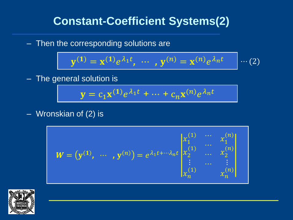
– Then the corresponding solutions are
– The general solution is
– Wronskian of (2) is
Constant-Coefficient Systems(2)

– We can graph solutions of (1), 𝐲 𝑡 =𝑦1(𝑡)𝑦2(𝑡)
as a single curve in the
𝑦1- 𝑦2 plane.
– That curve is a parametric representation with parameter 𝑡, and
called a trajectory of (1).
– The 𝑦1- 𝑦2 plane is called the phase plane.
– If we fill the phase plane with trajectories, we obtain the so-called
phase portrait of (1)
How to graph solutions in the phase plane
𝐲′ = 𝐀𝐲⇒𝑦1′ = 𝑎11𝑦1 + 𝑎12𝑦2
𝑦2′ = 𝑎21𝑦1 + 𝑎22𝑦2
⋯(1)

– By substituting 𝐲 = 𝐱𝑒𝜆𝑡 and 𝐲′ = 𝜆𝐱𝑒𝜆𝑡, we get 𝐀𝐱 = 𝜆𝐱.
– Characteristic equation
⇒ det(𝐀 − 𝜆𝐈) =−3 − 𝜆 1
1 −3 − 𝜆= 𝜆2 + 6𝜆 + 8 = 0
⇒ 𝜆1 = −2, 𝜆2 = −4
– For 𝜆1 = −2, 𝐱(𝟏) = 𝟏 𝟏 𝑻, and for 𝜆2 = −4, 𝐱(𝟐) = 𝟏 −𝟏 𝑻
– The general solution is
Phase portrait : example (1)
𝐲′ = 𝐀𝐲 =−3 11 −3
𝐲 ⇒𝑦1′ = −3𝑦1 + 𝑦2𝑦2′ = 𝑦1 − 3𝑦2
𝐲 =𝑦1𝑦2
= 𝑐1𝐲(1) + 𝑐2𝐲
(2) = 𝑐111𝑒−2𝑡 + 𝑐2
1−1
𝑒−4𝑡
⋯(1)

– Phase portrait of (1)
– The point 𝐲 = 𝟎 is a common point of all
projectories.
– Unique tangent direction for every point (𝑦1, 𝑦2)
except for the point (0, 0).
– This point (0, 0), at which 𝒅𝒚𝟐/𝒅𝒚𝟏 is undetermined, is called
a critical point.
Phase portrait : example (1)
𝑑𝑦2𝑑𝑦1
=𝑦2′𝑑𝑡
𝑦1′𝑑𝑡
=𝑎21𝑦1 + 𝑎22𝑦2𝑎11𝑦1 + 𝑎12𝑦2

– Improper node (two distinct real eigenvalues of the same sign)
: a critical point 𝑃0 at which all the trajectories, except for two of them,
have the same limiting direction of the tangent. The two exceptional
trajectories also have a limiting direction of the tangent at 𝑃0 which,
however, is different
Five types of critical points
𝐲′ =−3 11 −3
𝐲
⇒ 𝐲 = 𝑐111𝑒−2𝑡 + 𝑐2
1−1
𝑒−4𝑡

– Proper node (two identical eigenvalues and two linearly independent
eigenvectors)
: a critical point 𝑃0 at which every trajectory has a definite limiting
direction and for any given direction 𝒅 at 𝑃0 there is a trajectory
having 𝒅 as its limiting direction.
Five types of critical points
𝐲′ =1 00 1
𝐲
⇒ 𝐲 = 𝑐110𝑒𝑡 + 𝑐2
01𝑒𝑡 or 𝑐1𝑦2 = 𝑐2𝑦1
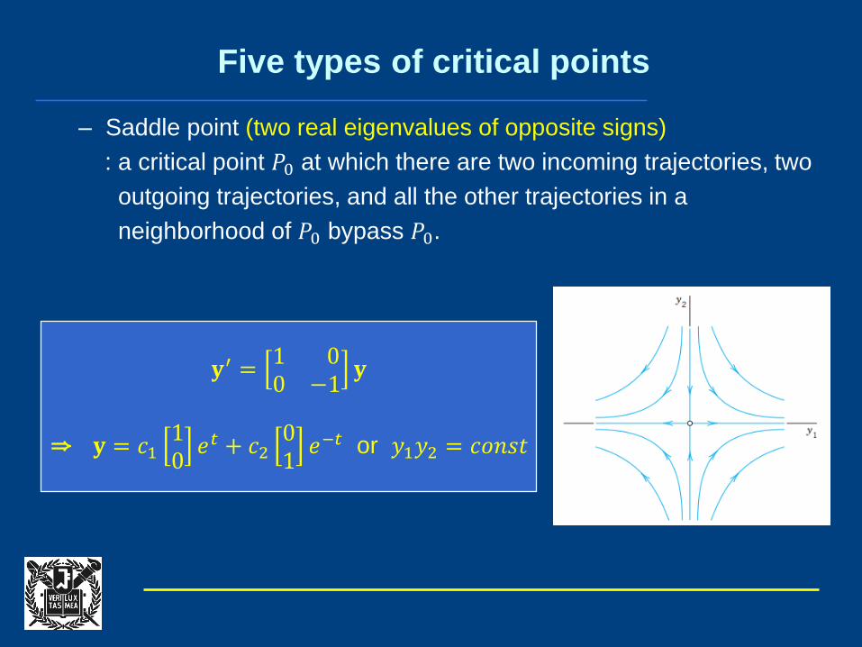
– Saddle point (two real eigenvalues of opposite signs)
: a critical point 𝑃0 at which there are two incoming trajectories, two
outgoing trajectories, and all the other trajectories in a
neighborhood of 𝑃0 bypass 𝑃0.
Five types of critical points
𝐲′ =1 00 −1
𝐲
⇒ 𝐲 = 𝑐110𝑒𝑡 + 𝑐2
01𝑒−𝑡 or 𝑦1𝑦2 = 𝑐𝑜𝑛𝑠𝑡

– Center (two purely imaginary conjugate eigenvalues)
: a critical point 𝑃0 that is enclosed by infinitely many closed
trajectories.
Five types of critical points
𝐲′ =0 1
−4 0𝐲
⇒ 𝐲 = 𝑐112𝑖
𝑒2𝑖𝑡 + 𝑐20−2𝑖
𝑒−2𝑖𝑡
or 2𝑦12 +
1
2𝑦22 = 𝑐𝑜𝑛𝑠𝑡

– Spiral point (two complex conjugate eigenvalues)
: a critical point 𝑃0 about which the trajectories spiral, approaching 𝑃0as 𝑡 → ∞ (or tracing these spirals in the opposite sense, away from
𝑃0).
Five types of critical points
𝐲′ =−1 1−1 −1
𝐲
⇒ 𝐲 = 𝑐11𝑖𝑒(−1+𝑖)𝑡 + 𝑐2
1−𝑖
𝑒(−1−𝑖)𝑡
or 𝑟 = 𝑐𝑒−𝑡 where 𝑟2 = 𝑦12 + 𝑦2
2

– Two identical eigenvalues and one eigenvector
– 𝐲(1) =1
−1𝑒3𝑡, and let 𝐲(2) = 𝐱𝑡𝑒3𝑡 + 𝐮𝑒3𝑡
– Then 𝐲 2 ′= 𝐱𝑒3𝑡 + 3𝐱𝑡𝑒3𝑡 + 3𝐮𝑒3𝑡 - (*)
𝐀𝐲 2 = 𝐀𝐱𝑡𝑒3𝑡 + 𝐀𝐮𝑒3𝑡 - (**)
⇒ 𝐀 − 𝟑𝐈 𝐮 = 𝐱, 𝐮 = 0 1 𝑇 (linearly independent of 𝐱)
⇒ 𝐲 = 𝑐11
−1𝑒3𝑡 + 𝑐2
1−1
𝑡 +01
𝑒3𝑡
Degenerate node
𝐲′ =4 1
−1 2𝐲 ⇒ 𝜆1 = 𝜆𝟐 = 𝜆 = 3, 𝐱1 = 𝐱2 = 𝐱 = 1 − 1 𝑇
(*)=(**) where 𝐀 =4 1
−1 2

Stability
– A critical point 𝑃0 is called stable if all trajectories that at some
instant are close to 𝑃0 remain close to 𝑃0 at all future times
– For every disk 𝐷 of radius 휀 > 0 with center 𝑃0 there is a disk 𝐷𝛿 of
radius 𝛿 > 0 with center 𝑃0 such that every trajectory that has a point
𝑃1(corresponding to 𝑡 = 𝑡1 say) in 𝐷 has all its points corresponding
to 𝑡 ≥ 𝑡1 in 𝐷 .
Criteria for critical points & stability
Stable critical point 𝑃0(The trajectory initiating at 𝑃1stays in the disk of radius 휀.)
Stable and attractive
critical point 𝑃0

𝐲′ = 𝐀𝐲 =𝑎11 𝑎12𝑎21 𝑎22
𝐲Ch. eqn. det 𝐀 − 𝜆𝐈 = 𝜆2 − 𝑎11 + 𝑎22 𝜆 + det𝐀
⇒ 𝑝 = 𝑎11 + 𝑎22, 𝑞 = det𝐀, Δ = 𝑝2 − 4𝑞
𝑝 = 𝜆1 + 𝜆2, 𝑞 = 𝜆1𝜆2, Δ = 𝜆1 − 𝜆22
Stability criteria for critical points
Eigenvalue criteria for critical points
Stability chart
Criteria for critical points & stability

Stability of critical points : Example
– Free motions of a mass on a spring
𝑚𝑦′′ + 𝑐𝑦′ + 𝑘𝑦 = 0
𝐲′ =0 1
−𝑘/𝑚 −𝑐/𝑚𝐲
𝑦1 = 𝑦𝑦2 = 𝑦′
det 𝐀 − 𝜆𝐈 = 𝜆2 + 𝑐/𝑚 𝜆 + 𝑘/𝑚 = 0𝑝 = −𝑐/𝑚, 𝑞 = 𝑘/𝑚, Δ = 𝑐/𝑚 2 − 4𝑘/𝑚
No damping (𝑐 = 0)
𝑝 = 0, 𝑞 > 0 ⇒ a center
Underdamping (𝑐2 < 4𝑚𝑘)
𝑝 < 0, 𝑞 > 0, Δ < 0⇒ a stable and attractive spiral point
Critical damping (𝑐2 = 4𝑚𝑘)
𝑝 < 0, 𝑞 > 0, Δ = 0⇒ a stable and attractive node
Overdamping (𝑐2 > 4𝑚𝑘)
𝑝 < 0, 𝑞 > 0, Δ > 0⇒ a stable and attractive node

Linearization of nonlinear systems
– If 𝑓1 and 𝑓2 in (1) are continuous and have continuous partial
derivatives in a neighborhood of the critical point 𝑃0: (0, 0), and if
det 𝐀 ≠ 0 in (2), then the kind and stability of the critical point of (1)
are the same as those of the linearized system
– Exception : 𝐀 has equal and pure imaginary eigenvalues
⇒ same kind of critical points of (3) or a spiral point
𝐲′ = 𝐟(𝐲) ⇒𝑦1′ = 𝑓1(𝑦1, 𝑦2)
𝑦2′ = 𝑓2(𝑦1, 𝑦2)
⋯ (1)Nonlinear
system
𝐲′ = 𝐀𝐲 + 𝐡(𝐲) ⇒𝑦1′ = 𝑎11𝑦1 + 𝑎12𝑦2 + ℎ1(𝑦1, 𝑦2)
𝑦2′ = 𝑎21𝑦1 + 𝑎22𝑦2 + ℎ2(𝑦1, 𝑦2)
⋯(3)𝐲′ = 𝐀𝐲 ⇒𝑦1′ = 𝑎11𝑦1 + 𝑎12𝑦2
𝑦2′ = 𝑎21𝑦1 + 𝑎22𝑦2

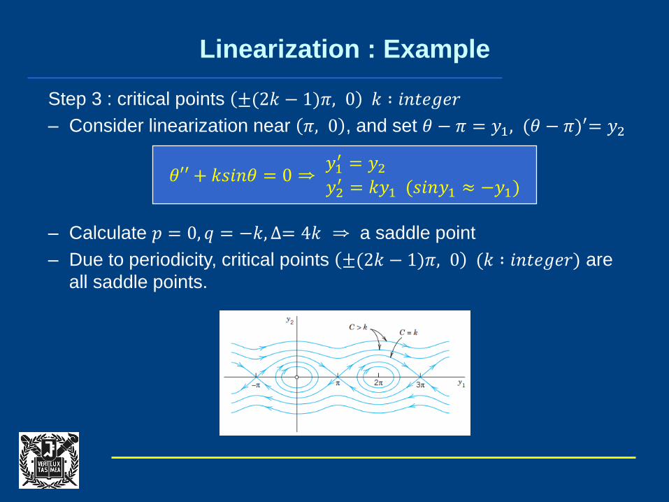
Linearization : Example
Free undamped pendulum
Step 1 : modeling
Step 2 : critical points ±2𝑘𝜋, 0 𝑘 ∶ 𝑖𝑛𝑡𝑒𝑔𝑒𝑟
– Consider linearization near 0, 0 , and set 𝜃 = 𝑦1, 𝜃′ = 𝑦2
– Calculate 𝑝 = 0, 𝑞 = 𝑘, ∆= −4𝑘 ⇒ a center
– Due to periodicity, critical points ±2𝑘𝜋, 0 (𝑘 ∶ 𝑖𝑛𝑡𝑒𝑔𝑒𝑟) are all
centers.
𝑚𝐿𝜃′′ + 𝑚𝑔𝑠𝑖𝑛𝜃 = 0 ⇒ 𝜃′′ + 𝑘𝑠𝑖𝑛𝜃 = 0 (𝑘 = 𝑔/𝐿)
𝜃′′ + 𝑘𝑠𝑖𝑛𝜃 = 0⇒𝑦1′ = 𝑦2
𝑦2′ = −𝑘𝑦1 (𝑠𝑖𝑛𝑦1 ≈ 𝑦1)
Linearization : Example
Step 3 : critical points ±(2𝑘 − 1)𝜋, 0 𝑘 ∶ 𝑖𝑛𝑡𝑒𝑔𝑒𝑟
– Consider linearization near 𝜋, 0 , and set 𝜃 − 𝜋 = 𝑦1, (𝜃 − 𝜋)′= 𝑦2
– Calculate 𝑝 = 0, 𝑞 = −𝑘, ∆= 4𝑘 ⇒ a saddle point
– Due to periodicity, critical points ±(2𝑘 − 1)𝜋, 0 (𝑘 ∶ 𝑖𝑛𝑡𝑒𝑔𝑒𝑟) are
all saddle points.
𝜃′′ + 𝑘𝑠𝑖𝑛𝜃 = 0⇒𝑦1′ = 𝑦2
𝑦2′ = 𝑘𝑦1 (𝑠𝑖𝑛𝑦1 ≈ −𝑦1)

Transformation to a 1st order eq. in the phase plane
– 2nd order autonomous ODE(an ODE in which 𝑡 does not occur explicitly)
– Take 𝑦 = 𝑦1 as the independent variable, set 𝑦′ = 𝑦2 and transform 𝑦′′
by the chain rule.
– Then, the ODE becomes of first order.
𝐹 𝑦, 𝑦′, 𝑦′′ = 0
𝑦′′ = 𝑦2′ =
𝑑𝑦2𝑑𝑡
=𝑑𝑦2𝑑𝑦1
𝑑𝑦1𝑑𝑡
=𝑑𝑦2𝑑𝑦1
𝑦2
𝐹 𝑦1, 𝑦2,𝑑𝑦2𝑑𝑦1
𝑦2 = 0

Example
Free undamped pendulum
– set 𝜃 = 𝑦1, 𝜃′ = 𝑦2
– Using separation of variables, we get
𝑚𝐿𝜃′′ + 𝑚𝑔𝑠𝑖𝑛𝜃 = 0 ⇒ 𝜃′′ + 𝑘𝑠𝑖𝑛𝜃 = 0 (𝑘 = 𝑔/𝐿)
𝜃′′ + 𝑘𝑠𝑖𝑛𝜃 = 0 ⇒𝑑𝑦2
𝑑𝑦1𝑦2 = −𝑘𝑠𝑖𝑛𝑦1
1
2𝑦22 = 𝑘𝑐𝑜𝑠𝑦1 + 𝐶 ⇒
1
2𝑚 𝐿𝑦2
2 −𝑚𝐿2𝑘𝑐𝑜𝑠𝑦1 = 𝑚𝐿2𝐶

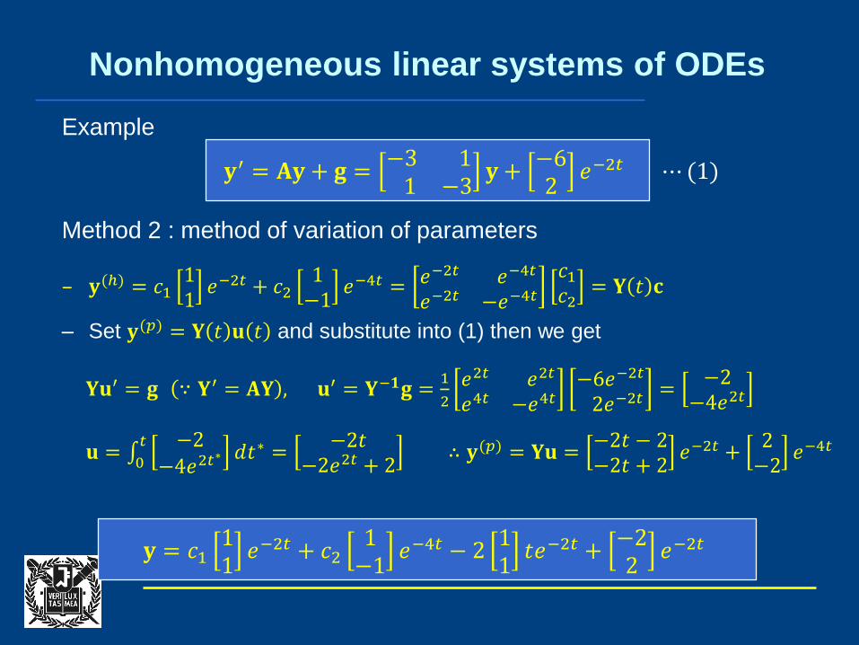
Nonhomogeneous linear systems of ODEs
Example
Method 1 : method of undetermined coefficients
– 𝐲(ℎ) = 𝑐111𝑒−2𝑡 + 𝑐2
1−1
𝑒−4𝑡
– Set 𝐲(𝑝) = 𝐮𝑡𝑒−2𝑡 + 𝐯𝑒−2𝑡 (by modification rule) where 𝐮 = 𝑎 1 1 𝑇
– Substitute 𝑦(𝑝) into (1), then we get
𝐮 − 2𝐯 = 𝐀𝐯 +−62
⇒𝑎𝑎
−2𝑣12𝑣2
=−3𝑣1 + 𝑣2
𝑣1 − 3𝑣2+
−62
⇒ 𝑎 = −2, 𝑣1 = 𝑘, 𝑣2 = 𝑘 + 4
– We can choose any real number 𝑘, like 𝑘 = 0
𝐲′ = 𝐀𝐲 + 𝐠 =−3 11 −3
𝐲 +−62
𝑒−2𝑡 ⋯(1)
𝐲 = 𝑐111𝑒−2𝑡 + 𝑐2
1−1
𝑒−4𝑡 − 211𝑡𝑒−2𝑡 +
04𝑒−2𝑡
Nonhomogeneous linear systems of ODEs
Example
Method 2 : method of variation of parameters
– 𝐲(ℎ) = 𝑐111𝑒−2𝑡 + 𝑐2
1−1
𝑒−4𝑡 = 𝑒−2𝑡 𝑒−4𝑡
𝑒−2𝑡 −𝑒−4𝑡𝑐1𝑐2
= 𝐘 𝑡 𝐜
– Set 𝐲(𝑝) = 𝐘 𝑡 𝐮 𝑡 and substitute into (1) then we get
𝐘𝐮′ = 𝐠 ∵ 𝐘′ = 𝐀𝐘 , 𝐮′ = 𝐘−𝟏𝐠 =1
2
𝑒2𝑡 𝑒2𝑡
𝑒4𝑡 −𝑒4𝑡−6𝑒−2𝑡
2𝑒−2𝑡=
−2−4𝑒2𝑡
𝐮 = 0𝑡 −2−4𝑒2𝑡
∗ 𝑑𝑡∗ =−2𝑡
−2𝑒2𝑡 + 2∴ 𝐲(𝑝) = 𝐘𝐮 =
−2𝑡 − 2−2𝑡 + 2
𝑒−2𝑡 +2−2
𝑒−4𝑡
𝐲′ = 𝐀𝐲 + 𝐠 =−3 11 −3
𝐲 +−62
𝑒−2𝑡 ⋯(1)
𝐲 = 𝑐111𝑒−2𝑡 + 𝑐2
1−1
𝑒−4𝑡 − 211𝑡𝑒−2𝑡 +
−22
𝑒−2𝑡
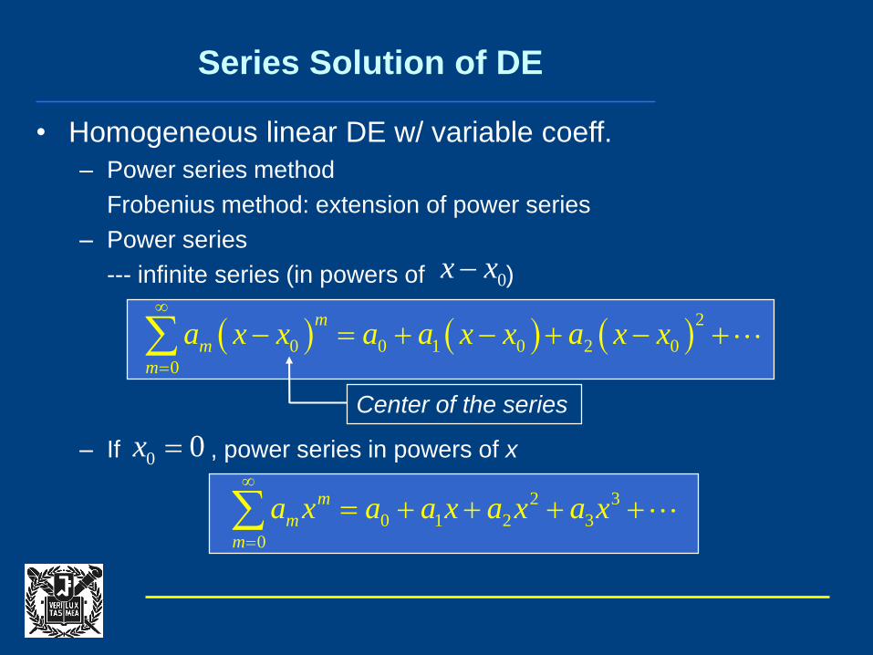
• Homogeneous linear DE w/ variable coeff.
– Power series method
Frobenius method: extension of power series
– Power series
--- infinite series (in powers of )
– If , power series in powers of x
Series Solution of DE
0x x
2
0 0 1 0 2 0
0
m
m
m
a x x a a x x a x x
Center of the series
0 0x
2 3
0 1 2 3
0
m
m
m
a x a a x a x a x

Maclaurin Series
2
0
2 3
0
2 2 4
0
2 1 3 5
0
11
1
1! 2! 3!
1cos 1
2 ! 2! 4!
1sin
2 1 ! 3! 5!
m
m
mx
m
m m
m
m m
m
x x xx
x x xe x
m
x x xx
m
x x xx x
m

– Represent p(x) and q(x) as a power series of x (or )
– Assume a sol. in the form of power series
– Collect like powers of x, and solve for the coefficients.
Power Series Method
0y p x y q x y
0x x
2 3
0 1 2 3
0
m
m
m
y a x a a x a x a x
1 2
1 2 3
0
2 3
m
m
m
y ma x a a x a x
2 2
2 3 4
0
1 2 3 2 4 3
m
m
m
y m m a x a a x a x
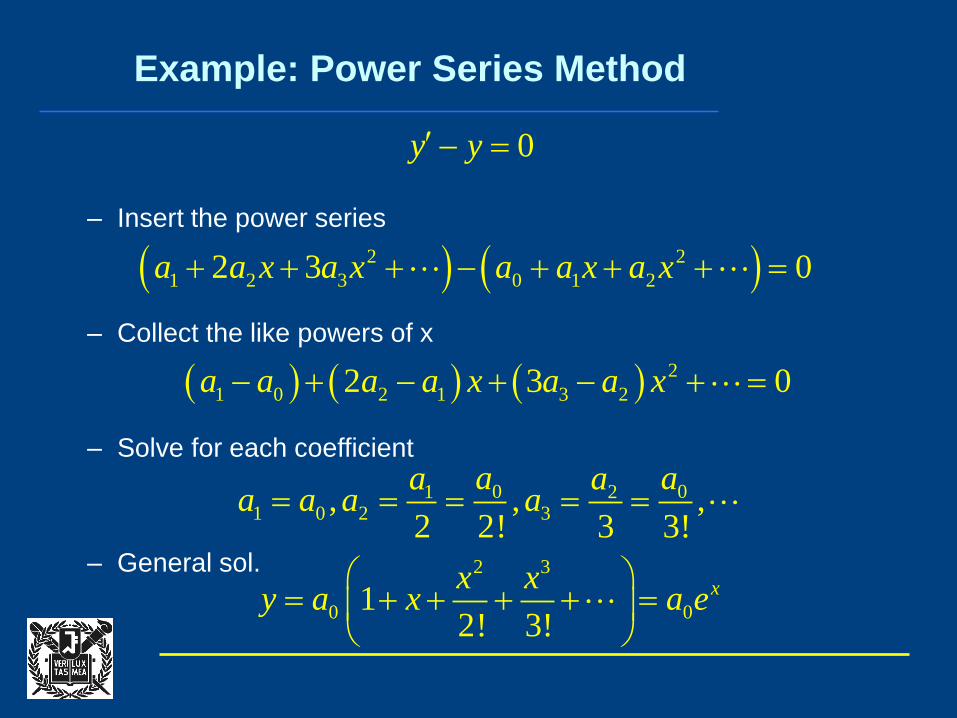
– Insert the power series
– Collect the like powers of x
– Solve for each coefficient
– General sol.
Example: Power Series Method
0y y
2 2
1 2 3 0 1 22 3 0 a a x a x a a x a x
2
1 0 2 1 3 22 3 0 a a a a x a a x
0 01 21 0 2 3, , ,
2 2! 3 3!
a aa aa a a a
2 3
0 012! 3!
xx xy a x a e
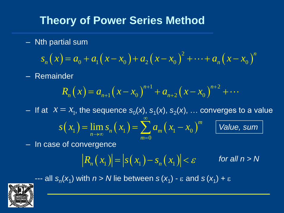
– Nth partial sum
– Remainder
– If at , the sequence s0(x), s1(x), s2(x), … converges to a value
– In case of convergence
--- all sn(x1) with n > N lie between s (x1) - and s (x1) +
Theory of Power Series Method
2
0 1 0 2 0 0 n
n ns x a a x x a x x a x x
1 2
1 0 2 0
n n
n n nR x a x x a x x
1x x
1 1 1 0
0
lim
m
n mn
m
s x s x a x x Value, sum
1 1 1 n nR x s x s x for all n > N

Convergence Interval (1)
– Always converges at . If it is the only point of convergence, all
other terms except a0 are zeros.
– Further values of x for convergence
0x x
Practically no interest
Convergence interval
0 x x R
Radius of convergence1
lim
m
mm
Ra

Convergence Interval (2)
If the limit is infinite, the power series only converges at .
– If the limit is 0, the power series converges for all x.
– Example: geometric series
--- geometric series converges and represents when
1
1
lim
m
mm
Ra
a
0x x
R
2
0
11
1
m
m
x x xx
1, 1 ma R
1x 1 1 x

Operations on Power Series (1)
– Term-wise differentiation
– Term-wise addition
0
0
m
m
m
y x a x x
1
0
0
m
m
m
y x ma x x
2
0
0
1
m
m
m
y x m m a x x
0 x x R
0 0
0 0
,
m m
m m
m m
a x x b x x
0
0
m
m m
m
a b x x

Operations on Power Series (2)
– Term-wise multiplication
– Vanishing of all coefficients
--- a positive radius of convergence, a sum is identically zero.
– Shifting summation indices
0 0
0 0
,
m m
m m
m m
a x x b x x
0 1 1 0 0
0
m
m m m
m
a b a b a b x x
2
0 0 0 1 1 0 0 0 2 1 1 2 0 0 a b a b a b x x a b a b a b x x
2 2 1
2 1
1 2
m m
m m
m m
x m m a x ma x

Operations on Power Series (3)
– Shifting summation indices (cont’d)
– Set
– Existence of power series sol.
--- if p(x), q(x), r(x) can be represented as a power series at ,
then every sol. is analytic.
1
2 1
1 2
m m
m m
m m
m m a x ma x
1, 1 s m m s
1
2 0
1 2 1
s s
s s
s s
s s a x s a x
1
2
1 2 1
s
s s
s
s s a s a x
0x x

Legendre’s Eqn. & Polynomials (1)
--- boundary value problems for spheres
– Sol.: Legendre function
– Since the coeff.’s are analytic, power series method can be applied.
Apply
21 2 1 0 x y xy n n y
Theory of special functions
0
m
m
m
y a x
2 2 1
0 0 0
1 1 2 0
m m m
m m m
m m m
x m m a x x ma x k a x

Legendre’s Eqn. & Polynomials (2)
– Arranging each power
– Coeff. of each power must be zero.
2
0 0
1 1 0
m m
m m
m m
m m a x m m a x
2
2 3 4 22 1 3 2 4 3 2 1 s
sa a x a x s s a x2
22 1 a x
2
1 22 1 2 2 1 s
sa x a x s s a x2
0 1 2 2 0 s
ska ka x ka x sa x
22 1 0 a n n
3 16 2 1 0 a n n a
0x
1x
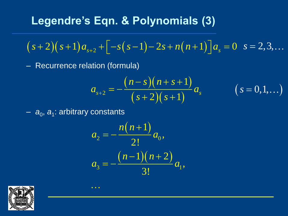
Legendre’s Eqn. & Polynomials (3)
– Recurrence relation (formula)
– a0, a1: arbitrary constants
22 1 1 2 1 0 s ss s a s s s n n a 2,3,s
2
1
2 1
s s
n s n sa a
s s
2 0
3 1
1,
2!
1 2,
3!
n na a
n na a
0,1,s

Legendre’s Eqn. & Polynomials (4)
– General sol.
– Converges for
– y1, y2: linearly independent
0 1 1 2 y a y x a y x
2 4
1
1 2 1 31
2! 4!
n n n n n ny x x
3 5
2
1 2 3 1 2 4
3! 5!
n n n n n ny x x x
1x

Legendre Polynomials (1)
– n is a nonnegative integer in many applications. Then, when s = n,
an+2 = 0, an+4 = 0, an+6 = 0, · · ·.
– If n is even, y1 reduces to a polynomial of degree n
– If n is odd, y2 reduces to a polynomial of degree n
– All the nonvanishing coeff. can be represented in terms of an
– an is arbitrary, and choose an = 1 when n = 1
Legendre polynomials
2
2 1
1s s
s sa a
n s n s
2s n
2
2 ! 1 3 5 2 1,
!2 !n n
n na
nn
1,2,n

Legendre Polynomials (2)
– Then,
– In general, when n – 2m ≥ 0
– Pn(x): Legendre polynomial of degree n
2
2 2 !,
2 1 ! 2 !n n
na
n n
4
2 4 !
2 2! 2 ! 4 !n n
na
n n
2
2 2 !1
2 ! ! 2 !
m
n m n
n ma
m n m n m
2
0
2
2
2 2 !1
2 ! ! 2 !
2 ! 2 2 !
2 1! 1 ! 2 !2 !
Mm n m
n nm
n n
nn
n mP x x
m n m n m
n nx x
n nn

Legendre Polynomials (3)
0
2
2
4 2
4
1
3
3
5 3
5
1,
13 1 ,
2
135 30 3 ,
8
1,
15 3 ,
2
163 70 15 ,
8
P x
P x x
P x x x
P x
P x x x
P x x x x
– First few of the functions

Legendre Polynomials (4)