Considerations on yield, nutrient uptake, cellular growth, and

competition in chemostat models

Julien Arino1 Sergei S. Pilyugin2 Gail S.K. Wolkowicz1

Abstract

We investigate some properties of a very general model of growth in the chemostat. In the classicalmodels of the chemostat, the function describing cellular growth is assumed to be a constant multipleof the function modeling substrate uptake. The constant of proportionality is called the growth yieldconstant. Here, this assumption of a constant describing growth yield is relaxed. Instead, we assumethat the relationship between uptake and growth might depend on the substrate concentration andhence that the yield is variable.

We obtain criteria for the stability of equilibria and for the occurrence of a Hopf bifurcation. Inparticular, a Hopf bifurcation can occur if the uptake function is unimodal. Then, in this setting, weconsider competition in the chemostat for a single substrate, in order to challenge the principle ofcompetitive exclusion.

We consider two examples. In the first, the function describing the growth process is monotoneand in the second it is unimodal. In both examples, in order to obtain a Hopf bifurcation, one ofthe competitors is assumed to have a variable yield, and its “uptake” is described by a unimodalfunction. However, the interpretation is different in each case. We provide a necessary condition forstrong coexistence and a sufficient condition that guarantees the extinction of one or more species.We show numerically by means of bifurcation diagrams and simulations, that the competitive ex-clusion principle can be breached resulting in oscillatory coexistence of more than one species, thatcompetitor-mediated coexistence is possible, and that these simple systems can have very complicateddynamics.

1 Introduction

Numerous papers deal with the growth of microorganisms in the chemostat. Most originate from bio-engineering and microbiology, where the chemostat finds a wide variety of applications, from theoreticalstudies of bacteria to the use of bacteria in biological waste decomposition and water purification (see,e.g., [6, 25]). As well as being an experimental system that generates reproducible results, it has beenmodeled extensively with good success. When browsing the corpus of literature dedicated to modelingthe chemostat, it appears that although approaches and applications are varied, most of the models relyon a simple relationship between two fundamental processes, nutrient uptake and cellular growth. In par-ticular, in most models these processes are assumed to be proportional. The constant of proportionalityis referred to as the growth yield constant or yield constant.

1Department of Mathematics, McMaster University, Hamilton, ON, Canada L8S 4K72Department of Mathematics, University of Florida, Gainesville, FL 32611-8105, USA

1

The notion of yield dates from the beginning of continuous bacterial culture, and is for exampledefined by Monod [24] as the ratio K of the amount of bacterial substance formed per amount of limitingnutrient utilized. He notes that if the growth is expressed as “standard” cell concentration, then 1/Krepresents the amount of limiting nutrient used up in the formation of a “standard” cell. He also notesthat the yield has, for a given strain and a given compound and under similar conditions, a remarkabledegree of stability and reproducibility. But this reasoning is based on the assumption of constant yield.

In most of the early models of microbial growth in the chemostat, besides assuming constant yield,it was assumed that growth was a monotone increasing function of substrate concentration. However,for some organisms, high concentrations of substrate can be detrimental, as was pointed out in 1925 byBriggs and Haldane [3]. See also [32] for a comprehensive review of the mechanisms involved. Inhibitionwas subsequently incorporated into models of bacterial growth (see, e.g., [2, 11]). Attempting to fitexperimental data, many authors have used different functional forms to model inhibition (see, e.g.,[9, 22, 29]).

Under the assumption of constant yield, mathematical models predict that there can be no sustainedoscillations (see, e.g., [5, 15, 30, 34]). Since such oscillations have been observed in experiments (see, e.g.,[10] for Arthrobacter globiformis and [18] for Lactobacillus plantarum), it is then useful to find modelsthat reproduce these oscillations.

With this in mind, we explore models involving variable yield. In the case of batch experiments, itwas shown [19] that oscillatory solutions occur only if the yield is a function of both the substrate andthe cell concentration. In continuous culture, this is not necessary, and most of the work has focusedon the simpler assumption of a substrate dependent yield. Different explanations can be given for thisdependence. In the case of chemical reactors, the yield is obtained from mass balance equations. Forbiological reactors, it is more complicated. See [31] for a recent review of various thermodynamicalmodels. For a description of how units of substrate are converted into units for cellular (bio)mass, see[25, p. 28-38].

The earliest model considering a more accurate relationship between uptake and growth was developedby Koga and Humphrey [16]. They introduce a respiration coefficient, R. They note that when respirationis considered, the observed yield coefficient Yobs is given by 1/Yobs = 1/Y +R/µ(S), where Y is a constantyield coefficient and µ(S) is the specific growth rate of the microorganisms. In subsequent work on thesubject, [7, 8, 13] assume that growth and uptake are related through a linear function of the substrateconcentration. In [1, 26, 27], linear and nonlinear functions modeling yield are considered and conditionsare derived for the existence of a Hopf bifurcation.

It is a difficult task to determine which part of the dynamics stems from the “higher” level processesthat are modeled, and which part stems from the nature of the hypotheses made on nutrient uptake andcellular growth. The objective of this paper is to explore the dynamics resulting from the different waysof modeling variable yield in the chemostat model. We review the commonly used methods describinguptake and growth, and study their interplay. To do this, we consider that the uptake, i.e., the processthrough which a cell absorbs nutrient, can be different from growth, i.e., the process through which a celltransforms the uptaken nutrient into biomass. However, we do not consider the effect of delay. We alsodo not consider long term nutrient storage directly.

The rest of this paper is organized as follows. In Section 2, we consider a very general model ofsingle species growth in the chemostat and first restrict our attention to what all such models have incommon. We give preliminary results, and in particular, show that the behavior of chemostat modelsabout the washout equilibrium point is generic. We are able to deal with the local stability analysis in thisvery general setting as well as some global properties of the model. Then we look for differences in thedynamics based on differences in the monotonicity assumptions on the nutrient uptake and cellular growth

2

and show that under certain assumptions Hopf bifurcation is possible, whereas under other assumptionsit is not. In Section 3, we briefly discuss the yield term and give different interpretations justifying asubstrate dependent yield function. In Section 4, we extend the model to the case of competing species.We provide a necessary condition for strong coexistence and a sufficient condition for the extinction ofa population. We give numerical evidence indicating that, unlike in the constant yield case, assuming avariable yield can lead to rather complicated dynamics and give numerical evidence that indicates thatthe principle of competitive extinction need not hold and that competitor-mediated coexistence seems tobe possible.

2 The general model for single species growth in a chemostat

Consider the following model of a chemostat in which a microbial species, with concentration (or biomass)at time t denoted x(t), consumes a single substrate with concentration S(t) at time t.

dS

dt= D(S0 − S) − xu(S) (1a)

dx

dt= x (g(S) − D1) (1b)

S(0) ≥ 0, x(0) ≥ 0

S0 denotes the substrate concentration in the input feed, and D denotes the dilution rate. We assumeonly that D1 > 0 and we make no assumption on the relative values of D and D1. However, the mostcommon interpretation for D1 is that it is the sum of the dilution rate and the species specific deathrate. Substrate is consumed by cells at the rate u(S(t)). This results in growth of the cellular biomassat the rate g(S(t)). The functions u and g are assumed to be continuously differentiable. The uptakefunction u(S) is further assumed to satisfy u(0) = 0. By this, we mean that if there is no substrate inthe environment, then there is no substrate uptake. As mentioned earlier, we do not model storage ofnutrient directly and so in the absence of substrate, we assume that there is no growth so that g(0) = 0.Otherwise, u(S) and g(S) are positive for S > 0. Finally, we assume that each one of these functions iseither monotone increasing or unimodal.

2.1 Local analysis

The washout equilibrium, E0 ≡ (S0, 0), always exists.

Condition 2.1. E∗ ≡ (S∗, x∗) =(

S∗,D(S0 − S∗)

u(S∗)

), where S∗ is any solution of

g(S) = D1 (2)

is a feasible positive equilibrium if, and only if, S∗ < S0.

In what follows, we restrict our attention to functions u(S) and g(S) that are either monotone in-creasing or initially monotone increasing and unimodal. Thus, there are at most two values of S thatsatisfy (2). They are denoted λ, µ ∈ R, with λ < µ. We adopt the convention that µ = ∞ if (2) has onlyone solution, and λ = ∞ if (2) has no solution. Therefore, S∗ must equal either λ or µ. We refer to E∗

as E∗λ or E∗

µ when it is necessary to make the distinction. See Figure 1.

3

D

S

gM

g(S)

1

λ

(a)

D

S

M

g(S)

λ µ

g

1

(b)

Figure 1: Definition of λ and µ, in the case of (a) monotone growth (µ = ∞); (b) nonmonotone growth.

We are not aware of any experimental evidence of growth or uptake processes limited by a singlesubstrate that exhibit more complicated behavior (such as two-humped responses). A similar analysisfor more complicated functions is however possible, but involves treating more cases.

The Jacobian matrix evaluated at an arbitrary point (S, x) is given by[ −D − u′(S)x −u(S)g′(S)x g(S) − D1

]. (3)

Thus, the Jacobian matrix evaluated at the washout equilibrium, E0, is given by[ −D −u(S0)0 g(S0) − D1

]. (4)

Condition 2.2. The washout equilibrium, E0, is locally asymptotically stable if g(S0) − D1 < 0.

Evaluated at a positive equilibrium, E∗, the Jacobian matrix is[ −D − u′(S∗)x∗ −u(S∗)g′(S∗)x∗ 0

]. (5)

Thus, det(J) = u(S∗)g′(S∗)x∗ and Tr(J) = −D − u′(S∗)x∗. Since D, u, (S) and x∗ are positive, bythe Routh-Hurwitz criterion, we obtain the following condition.

Condition 2.3. A feasible positive equilibrium, E∗, is locally asymptotically stable if the following twoinequalities are satisfied simultaneously:

g′(S∗) > 0, and u′(S∗) > − u(S∗)S0 − S∗ . (6)

Another consequence of (5) is that the existence of complex eigenvalues, i.e., oscillations (both dampedand sustained), is determined by the following condition, which follows directly from the characteristicpolynomial of (5).

4

Condition 2.4. The linearization of (1) about a feasible positive equilibrium, E∗, has complex eigenvaluesif, and only if, (D + u′(S∗)x∗)2 < 4u(S∗)g′(S∗)x∗.

This implies that there are no oscillations in a neighborhood of a positive equilibrium, E∗, if g′(S∗) < 0.

Condition 2.5. The eigenvalues of the linearization (5) of system (1) about a positive equilibrium, E∗,are purely imaginary if, and only if,

g′(S∗) > 0, and u′(S∗) = − u(S∗)S0 − S∗ , (7)

Thus, a Hopf bifurcation of a locally asymptotically stable equilibrium point can only occur at anequilibrium, E∗

λ, since it is necessary that u′(S∗) < 0 and g′(S∗) > 0. Since the bifurcation requires g tobe increasing at S∗, it follows that S∗ must equal λ, not µ.

Select one of the parameters in the model as the bifurcation parameter and call it α.

Theorem 2.6. Assume that there exists α = αc, the critical value of α, such that x∗αc

u′(λαc) + D = 0.System (1) undergoes a Hopf bifurcation at E∗

λαc= (λαc , xαc) if g′(λαc) > 0 and

d

dα(−Dx∗(α)u′(S∗(α)))|α=αc

= 0. (8)

This bifurcation is supercritical if CH defined by

CH ≡ −u(λαc)g′(λαc)u

′′′(λαc) + u′′(λαc)(u′(λαc )g

′(λαc) + u(λαc)g′′(λαc))

is negative, and subcritical if CH > 0.Equivalently, the bifurcation is supercritical if the sign of

CH ≡ h′′′(λαc)u(λαc) + 2h′′(λαc)u′(λαc ) −

h′′(λαc)g′′(λαc)u(λαc)g′(λαc)

is negative, and subcritical if it is positive, where h(S) = (S0−S)Du(S) , the S-isocline.

The proof of this result follows from the formula derived in Marsden and McCracken [23] and ispostponed to Appendix A. Another technique for determining the criticality of the Hopf bifurcation inthis context is to use the divergence criterion as in [26] or the rescaling method as in [27].

2.2 Global analysis

2.2.1 Boundedness of solutions.

Lemma 2.7. Both the nonnegative cone and the interior of the nonnegative cone are positively invariantunder the flow of (1).

Proof. The line S ≥ 0, x = 0 is invariant under the flow of (1). Also, for S = 0 and x > 0, S′ = DS0 > 0,i.e., the vector field points strictly inwards.

Lemma 2.8. Solutions of (1) are defined and remain bounded for all t ≥ 0.

5

Proof. The proof is identical to the proof of Theorem 4.1 in Section 4 in the case that n = 1.

Lemma 2.9. For any ε > 0, there exists Tε ≥ 0 such that S(t) ≤ S0 + ε for all t ≥ Tε. If in addition,λ < S0, g(S) > D1 for S ∈ (λ, S0], and x(0) > 0, then there exists T such that S(t) < S0 for all t > T .

Proof. First suppose that x(0) = 0. Then, clearly S(t) converges to S0.Now assume that x(0) > 0. If there exists T ≥ 0 such that S(T ) = S0, then S′(T ) = −u(S(T ))x(T ) <

0. This implies that if there exists t ≥ 0 such that S(t) ≤ S0 then S(t) < S0 for all t > t. If S(t) > S0

for all t ≥ 0, then S′(t) < 0 for all t > 0. Therefore S(t) converges to some α ≥ S0. If α > S0, thenS′(t) < (S0 − α)D < 0 for all t > 0. But this implies that S(t) converges to −∞ as t tends to ∞, acontradiction. Therefore, either S(t) ≤ S0 for all sufficiently large t or S(t) converges to S0 as t → 0.

Now assume that λ < S0, g(S) > D1 for S ∈ (λ, S0], and x(0) > 0. Suppose S(t) > S0 for all t > 0.Then, by the continuity of g(S), there exists ∆ > S0 such that g(S) > D1 for all S ∈ [S0, ∆] and thereexists a T∆ > 0 such that S0 < S(t) < ∆ for all t > T∆. Define g ≡ minS∈[S0,∆] g(S). Then g > D1. But

then, since by Lemma 2.7, x(t) > 0 for all t > 0, x′(t)x(t) > (g − D1) > 0, for all t > T∆. Integrating both

sides from T∆ to ∞, it follows that x(t) → ∞. But, by Lemma 2.8, x(t) is bounded, a contradiction. Theresult follows.

2.2.2 Global stability of equilibrium points

Theorem 2.10. If S0 ≤ λ, then the washout equilibrium, E0, of (1), is globally asymptotically stable.

Proof. Since the nonnegative cone is invariant and all solutions are bounded, the result follows immedi-ately from a standard phase portrait analysis.

Theorem 2.11. If λ < S0, g′(λ) > 0, g(S0) > D1, u′(λ) > − u(λ)S0−λ and 1 − u(S)(S0−λ)

u(λ)(S0−S) has exactlyone sign change for S ∈ (0, S0), then the equilibrium, E∗

λ = (λ, x∗λ), is globally asymptotically stable with

respect to the interior of the positive cone.

Proof. First, note that since g(S0) > D1, it follows that λ < S0 ≤ µ, and so by Condition 2.1, E∗µ is not

feasible and that by Condition 2.3, E∗λ is locally asymptotically stable. Also, by Lemma 2.9, without loss

of generality, we need only consider S ∈ [0, S0].Consider the following function,

V (S, x) =∫ S

λ

(g(ξ) − D1)(S0 − λ)u(λ)(S0 − ξ)

dξ + x − x∗λ ln(

x

x∗λ

), (9)

that is defined and continuously differentiable for S ∈ (0, S0) and x > 0. For brevity of notation, let

Ψ(S) =u(S)

S0 − S. (10)

Then, using (10) it follows that

V = x(g(S) − D1)(

1 − u(S)(S0 − λ)u(λ)(S0 − S)

)= x(g(S) − D1)

(1 − Ψ(S)

Ψ(λ)

). (11)

6

Note that V = 0 if and only if S = λ or x = 0 or S = µ = S0. The derivative of Ψ is given byu′(S)(S0 − S) + u(S)

(S0 − S)2. From Condition 2.3 and by the continuity of u′, we have that for S close to λ,

u′(S)(S0 − S) + u(S) > 0, and thus the function Ψ is increasing. Also, g is monotone increasing for Snear λ. Since each term in (11) changes sign at S = λ, this implies that for S close to λ, V < 0. In fact,V remains negative as long as neither term in (11) changes sign. But this is ruled out by the hypotheses.

Let η = (S, x) ∈ [0, S0] : V (S, x) = 0. Therefore, η = (S, x) ∈ [0, S0] : x = 0 or S = λ or S = S0 =µ. Let E denote the largest invariant subset of η. Then E = (S, 0), 0 ≤ S ≤ S0∪E∗

λ. As solutions arebounded, E attracts all solutions with nonnegative initial conditions (by the modified LaSalle’s ExtensionTheorem, as stated in [34, Th. 1.2]). Noting that from our hypotheses, E0 is unstable and E∗

λ = (λ, x∗λ)

is locally asymptotically stable, using a standard argument involving the Butler-McGehee Lemma (see[30]), it follows that no points of the form (S, 0), S ≥ 0 can be in the omega limit set of any solutioninitiating inside the positive cone and so the result follows.

3 Discussion of the yield term

There are different mechanisms that lead to the use of a yield term in chemostat models. Consider thefollowing expression relating growth and uptake:

g(S) = ρu(S). (12)

As mentioned in the Introduction, one rationale for including the yield term is, historically, to expresssubstrate and organic biomass in the same units. In this case, the yield term is the constant of propor-tionality in (12).

Another use of the yield coefficient, often confused with the previous one, is to decribe the efficiencyof the processes involved. If substrate and microorganism were evaluated in the same units, a perfectreaction would transform one unit of substrate into one unit of microorganism. However, such reactionsare not perfect. It is for example possible, in the case of chemical reactions, to compute theoretical yieldvalues from the mass-balance equations of the reactions involved; see, e.g., [31]. It is then possible tostate that for a given reaction, it takes one mole of reactant to produce ρ moles of product. Equation(12) would in this case give the rate of formation of moles of the new compound as a function of thenumber of moles of the reactant. Again, in this case ρ would be a constant.

Things are more complicated for more complex processes. In particular, biological processes are proneto a lot of individual variability, making it more difficult to obtain a measure of the efficacy of a biologicalreaction. Since this measure is very important, for example in the bioprocess field where it serves as anindicator of the economic viability of a given process, the yield has been the object of numerous studies.However, a functional form for the yield has not yet been validated by experiment.

Formally, the yield is the ratio between the amount of matter taken up and the resulting cellulargrowth, and so it is likely that the yield is not actually constant, but could depend on the substrateconcentration, the microbial concentration, and environmental conditions among other things.

In the model studied by Crooke and Tanner [7] and Agrawal, Lee, and Ramkrishna [1], they assumedthat the yield is a function of the substrate concentration, Y (S). They considered monotone growth g(S)and modeled the uptake in system (1) by u(S) = g(S)/Y (S), where Y (S) = a + bS. They let

I. g(S) = µmSKm+S , and so u(S) = µmS

(a+bS)(Km+S) ,or

7

II. g(S) = kSe(− SK ), and so u(S) = kSe(− S

K)

(a+bS) .

Pilyugin and Waltman [27] proved that only super-critical Hopf bifurcations are possible in case I.However, if Y (S) = a+ bS2, they proved that both super- and sub-critical Hopf bifurcations are possible.

In the case of constant yield, including the yield term in the substrate equation is mathematicallyequivalent to including the reciprocal in the microorganism equation instead. One of the important dif-ferences in the case that the yield is not constant is that the variable yield term can lead to uptake andgrowth terms that have different monotonicity properties. Therefore, careful attention to the interpreta-tion of the yield term resulting in its correct placement in the equations is necessary. This is especiallytrue, since the explicit form of the yield function is not yet known. Thus, it is currently only possible torepresent the yield in the model using a function that we suspect has similar qualitative properties, e.g.,similar monotonicity properties.

If it is assumed that the yield is constant, but that cells need some maintenance energy, then in [16],the yield is given by :

−dS

dt=

1Y

dx

dt+ Rx,

where R can be interpreted, for example, as the portion of nutrient used for respiration. An alternativeapproach to modeling the maintenance energy is to consider the yield as a function of the substrateconcentration.

Modeling the yield as a function of substrate concentration could also provide an indirect way ofmodeling storage of nutrient. As well, Godin, Cooper, Rey [14] provide experimental evidence thatindicates that critical division mass increases as substrate concentration increases and so reproductionrate depends on substrate concentration.

The different interpretations of yield can lead to different forms for the yield functions and differentways to include the yield terms.

4 The general competition model

We consider the more general case of several species competing for a common resource using the frameworkof the previous sections. Here, xi(t) denotes the concentration of the ith population of microorganismsat time t.

dS

dt= D(S0 − S) −

n∑i=1

xiui(S) (13a)

dxi

dt= xi (gi(S) − Di) , i = 1, . . . , n, (13b)

S(0) ≥ 0, xi(0) ≥ 0, i = 1, . . . , n

For each species, we define the break-even concentrations λi and µi as in Section 2. In the case ofconstant yield, i.e. ui(S) is proportional to gi(S) for each i = 1, 2, . . . , n, if the species specific deathrates are assumed to be insignificant compared to the dilution rate (i.e. Di = D for all i or at least Di

sufficiently close to D for all i), the dynamics are well understood. See for example, [5, 30, 35]. Withconstant yield and monotone or inhibitory growth, the competitive exclusion principle holds. At mostone species avoids extinction, and its concentration rapidly approaches an equilibrium concentration. Inthe case of monotone response functions, the species that survives is the one with the lowest break-evenconcentration. Similar results hold in the case that Di may not equal D, see for example, [15, 20, 34, 35],

8

although this case is not yet completely understood. However, in the case of constant yield, numericalsimulations of model (13) to date have only displayed competitive exclusion with convergence to anequilibrium with at most one surviving species.

In the rest of this paper, we demonstrate that in the case of variable yield, more exotic dynamicalbehavior seems to be possible.

Before we consider specific examples we make the following observations.

Theorem 4.1. Both the nonnegative cone and the interior of the nonnegative cone are invariant underthe flow of (13) and all solutions are defined and remain bounded for all t ≥ 0.

Proof. An argument similar to that given to prove Lemma 2.7 can be used to establish that solutions arenonnegative and hence bounded below, so it remains only to prove that all solutions are bounded above.

Without loss of generality, assume that xi(0) > 0 and thus xi(t) > 0 for all i ∈ 1, ..., n and allt ≥ 0 in the domain of definition of the solution (S(t), x1(t), ..., xn(t)). Let S = max(S(0), S0). Then thenonnegativity of solutions implies that S(t) ≤ S for all t ≥ 0 for which S(t) is defined. Since gi(0) = 0,by the continuity of gi, there exists ε > 0 such that gi(S) ≤ Di

2 for all 0 ≤ S ≤ ε and all i ∈ 1, ..., n. Inaddition, there exists Mε > 0 such that

gi(S) − Di + D

ui(S)≤ Mε, ∀S ∈ [ε, S], ∀i ∈ 1, ..., n.

Let x > Mε(S − ε) and define Ω(x) to be the set

Ω(x) = (S, x1, ..., xn) ⊂ Rn+1+ : S ≤ S,

n∑i=1

xi ≤ min(x, x − Mε(S − ε)).

Choose x sufficiently large so that (S(0), x1(0), ..., xn(0)) ∈ Ω(x).We have already established that 0 ≤ S(t) ≤ S. If (S, x1, ..., xn) is a point on the relevant part of the

boundary of Ω(x), then either S < ε and∑n

i=1 xi = x, or ε ≤ S ≤ S and∑n

i=1 xi = x − Mε(S − ε). Inthe former case, we have that

( n∑i=1

xi

)′=

n∑i=1

xi(gi(S) − Di) ≤ −n∑

i=1

xiDi

2< 0,

since we assumed xi > 0. In the latter case, we have that

(S +

n∑i=1

xi

Mε

)′= D

(S0 − S −

n∑i=1

xi

Mε

)+

n∑i=1

xi

Mε

(−Mεui(S) + (gi(S) − Di + D)

).

Since ε ≤ S ≤ S, the choice of Mε warrants that

n∑i=1

xi

Mε

(−Mεui(S) + (gi(S) − Di + D)

)≤ 0.

Consequently, (S +

n∑i=1

xi

Mε

)′≤ D

(S0 − S −

n∑i=1

xi

Mε

)= D(S0 − ε − x

Mε) < 0,

9

because S0 ≤ S < ε + xMε

by the choice of x. We conclude that the vector field of (13) points strictlyinto the interior of Ω(x) when restricted to the part of the boundary ∂Ω with xi > 0, i = 1, 2, . . . , nand 0 ≤ S ≤ S. Also, since xi(0) > 0, we have that xi(t) > 0, for all i = 1, . . . , n, and t > 0. Thus(S(t), x1(t), ..., xn(t)) ∈ Ω(x) for all t ≥ 0. Since Ω is bounded, (S(t), x1(t), ..., xn(t)) must be boundedfor all t ≥ 0.

Lemma 4.2. In (13), if for some i ∈ 1, . . . , n, λi > S0, then xi(t) → 0 as t → ∞.

Proof. Using an argument similar to that given to prove Lemma 2.9, it follows that there exists ε > 0,and T > 0 such that S(t) < S0 + ε < λi, for all t ≥ T . By Lemma 4.1 xi(t) is nonnegative, and sox′

i(t)xi(t)

< −Di + gi(S0 + ε) < 0 = −Di + gi(λi), for all t > T . Integrating from t = T to ∞, it follows thatxi(t) → 0 as t → ∞.

The next two results are helpful for constructing examples in which coexistence is possible.

Theorem 4.3. Suppose that(i) there exist nonempty sets I−, I+ ⊂ 1, ..., n and αi > 0 such that I−

⋂I+ = ∅ and

G(S) =∑i∈I−

αi(gi(S) − Di) −∑i∈I+

αi(gi(S) − Di) < 0, for all S ∈ (0, S0); (14)

(ii) there exists j ∈ I+ such that gj(S0) > Dj.Then for any positive solution (S(t), x1(t), ..., xn(t)) of (13),

limt→∞

∏i∈I−

xαi

i (t) = 0.

Proof. By Theorem 4.1, there exists M > 0 such that 0 ≤ xi(t) ≤ M for all i = 1, ..., n and t ≥ 0.Equation (13a) then implies that there exists a sufficiently small δ > 0 such that S(t) ≥ δ for allsufficiently large t. By an argument similar to that given in Lemma 2.9, S(t) < S0 for all sufficientlylarge t. Therefore, there exists T > 0 such that 0 < δ < S(t) < S0 for all t > T .

For all i ∈ I−⋃

I+, define zi(t) = xαi

i (t). Then

z′i(t) = αixαi−1i (t) xi(t)(gi(S(t)) − Di) = zi(t) αi(gi(S(t)) − Di).

Let

ξ(t) =

∏i∈I− zi(t)∏i∈I+

zi(t),

thenξ′(t) = ξ(t)G(S(t)).

Since S(t) ∈ [δ, S0) for all t > T , G(S(t)) < 0 so that ξ(t) is a strictly decreasing function for t > Tbounded below by 0. It follows that there exists ξ0 = limt→∞ ξ(t) ≥ 0. Now there are two possibilities.The first possibility is that ξ0 = 0 in which case

0 ≤ limt→∞

∏i∈I−

zi(t) ≤( ∏

i∈I+

Mαi

)lim

t→∞ ξ(t) = 0.

10

The second possibility is that ξ0 > 0, in which case, a theorem by Hadamard and Littlewood [21] impliesthat limt→∞ G(S(t)) = 0. Since S(t) ∈ [δ, S0) for all t > T , it must be the case that limt→∞ S(t) = S0.But this conclusion would contradict the boundedness of xj(t) and hence the assertion ξ0 > 0 is invalid.The result follows by observing that

limt→∞

∏i∈I−

xαi

i (t) = limt→∞

∏i∈I−

zi(t) = 0.

Corollary 4.4. If the set I− is a singleton, that is, I− = i∗, then the assumptions (i) and (ii) implythat for any positive solution (S(t), x1(t), ..., xn(t)) of (13),

limt→∞xi∗(t) = 0.

In the population dynamics literature, two types of coexistence are distinguished: strong and weak.We say that a positive solution (S(t), x1(t), ..., xn(t)) exhibits strong coexistence if lim inft→∞ xi(t) > 0,for all i ∈ 1, ..., n and it exhibits weak coexistence if lim supt→∞ xi(t) > 0, for all i ∈ 1, ..., n. Usingthis terminology, Theorem 4.3 provides a necessary condition for strong coexistence. The conclusion that

limt→∞

∏i∈I−

xαi

i (t) = 0

is insufficient to eliminate the possibility of weak coexistence. We would like to point out that Raoand Roxin [28] have obtained an equivalent criterion for strong coexistence using the methods of controltheory for constant yields (gi(S) = kiui(S)) and a time dependent input feed concentration (S0 = S0(t)).

4.1 Yield included in the uptake equation

Here, we consider model (13) of the chemostat in which two microbial species x1 = x and x2 = y competefor a single substrate S. We assume that the species x has a variable yield while the species y has aconstant yield. As we pointed out previously, there are two ways to incorporate the variable yield into themodel. In this section we choose to incorporate the yield into the consumption (uptake) rate of speciesx. In addition, we assume that the variables x, y, and S, and time t, have been rescaled appropriately sothat both the dilution rate D and the substrate feed concentration S0 equal unity, that is, D = S0 = 1.The model then takes the form

dS

dt= 1 − S − x

p1(S)γ1(S)

− yp2(S)

γ2, (15a)

dx

dt= x(p1(S) − 1), (15b)

dy

dt= y(p2(S) − 1), (15c)

S(0) ≥ 0, x(0) ≥ 0, y(0) ≥ 0.

11

We assume that the specific growth rates p1(S) and p2(S) are expressed in the traditional Monodformulation

pi(S) =miS

ai + S, i = 1, 2,

and the variable yield coefficient of the species x is given by γ1(S) = b1 + c1Sn where b1, c1 > 0 and n is

a positive integer. For a more detailed description of the model (15) we refer the reader to [27].For reasons that will be explained below, we choose to treat c1 and m2 as bifurcation parameters.

The rest of the parameters will be fixed as shown in Table 1.

Table 1: Parameter values for model (15).m1 = 2.0 m2 variesa1 = 0.7 a2 = 6.5b1 = 1.0 γ2 = 120.0c1 varies n = 4

The break-even concentrations λi of the species x and y can be obtained by solving pi(λi) = 1:

λ1 =a1

m1 − 1= 0.7, λ2 =

a2

m2 − 1.

Since λ1 < 1, species x will persist in the absence of species y. A necessary condition for the species y topersist in the culture is that λ2 < 1, or equivalently, m2 > 7.5.

Corollary 4.4 implies that a necessary condition for coexistence is that the graphs of p1(S) and p2(S)intersect at some point 0 < S < 1. In model (15),

S =m1a2 − m2a1

m2 − m1

so that a necessary condition for coexistence is

8.82 = m1a2

a1< m2 < m1

a2 + 1a1 + 1

= 18.57.

If m2 < 8.82, then x will always drive y to extinction. If m2 > 18.57, then y will always drivex to extinction. Both of these conclusions hold regardless of any particular dynamic behavior of thefull system (e.g., equilibrium, periodic solution, or other) and specifically they are independent of thefunctional form of the variable yield coefficient γ1(S). If γ1(S) = γ1 were constant, then the outcome ofcompetition would be completely determined by the inequality λ1 < λ2 and whether or not λ < 1. Thecritical value of m2 for which λ1 = λ2 is given by m2 = 1 + (m1 − 1)a2

a1= 10.286.

4.1.1 Bifurcation to coexistence

The fact that single species continuous cultures with variable yields may exhibit sustained oscillations hasan important implication for coexistence. The principle of competitive exclusion states that two speciescannot coexist at equilibrium when they compete for a single substrate in continuous culture. The firstproof of this assertion was presented in [15] for Monod uptake rates and it was later extended to a muchbroader class of growth rates and uptake functions in [34]. In [4], a two predator - one prey ecosystem was

12

studied in the chemostat setting. It was shown that such a system may exhibit a stable periodic solutionwith both competing predators present at all times. Specifically, it was shown that the stable limit cyclecorresponding to sustained oscillations of a single predator population can bifurcate into the region ofcoexistence and preserve its stability. In [27], it was demonstrated that the same type of bifurcation canoccur in the chemostat when one competitor exhibits a variable yield and the other competitor has aconstant yield. If Γ = (S(t), x(t)) is a stable periodic solution of (15) of period T > 0 with y = 0, then Γundergoes a transcritical bifurcation when m2 increases past the bifurcation value

m∗2 =

T∫ T

0S(t)

a2+S(t) dt. (16)

The stable periodic solution of (15) with x(t), y(t) > 0 exists for m2 > m∗2.

If we let y = 0 in (15) then the reduced model (15a–15b) undergoes a Hopf bifurcation when c1 crossesthe value

c1 =(m1 − 1)4

((m1 − 1)2 + a1

)a41(3m2

1 − 4m1a1 − 2m1 − a1 − 1). (17)

For the parameter values given in Table 1, the Hopf bifurcation occurs at c1 = 10.115. Furthermore, theHopf bifurcation is supercritical for m2 = 2, a2 = 0.7, n = 4, that is, the stable limit cycle of (15a–15b)exists for c1 > c1.

To compute the bifurcation value m∗2 for different values of c1, we implemented the formula (16) as

follows. If c1 < c1 and the stable limit cycle of (15a–15b) does not exist, then we let

m∗2 =

a2 + λ1

λ1,

which is the limiting case of (16) as S(t) → λ1 and T → ∞. If c1 > c1, then the stable limit cycle Γ doesexist and we first integrate (15a–15b) with y = 0 in forward time to approximate Γ and then use (16) tofind m∗

2. The output of this numerical procedure is shown in Figure 2.In the remainder of this section, we present a numerical study of the dynamics exhibited by solutions

which correspond to competitive coexistence in the case λ1 < λ2 < 1, c > c and m2 > m∗2. Considering

the dynamics on the invariant planes Fx = S, x ≥ 0, y = 0 and Fy = x = 0, S, y ≥ 0, this is the casewhen almost all positive solutions correspond to coexistence, that is,

lim supt→∞

x(t) > 0, lim supt→∞

y(t) > 0.

To see this, let W s(E) and Wu(E) denote the stable and unstable manifold of the equilibrium E,respectively. Observe that both Fx and Fy contain the (trivial) equilibrium E0 = (1, 0, 0) which is asaddle with dimWu(E0) = 2. In addition, Fx contains the equilibrium E1 = (λ1, x

∗, 0) and Fy containsthe equilibrium E2 = (λ2, 0, y∗). Since y has a constant yield, E2 is a local attractor relative to Fy, thatis, dim W s(E2) = 2 with W s(E2) ⊂ Fy and the inequality λ1 < λ2 guarantees that dimWu(E2) = 1with Wu(E1) ⊂ R

3+. Thus, E1 repels towards the interior of R

3+. If c > c, then dimWu(E1) = 2 with

Wu(E1) ⊂ Fx and dimW s(E1) = 1 with W s(E1) ⊂ R3+. Furthermore, since c > c and m2 > m∗

2, thereexists an unstable limit cycle Γ sitting in Fx that is a saddle with respect to R3. It is attracting in Fx,but repels into the interior of R

3 and dim W s(Γ) = 2, dim Wu(Γ) = 2, and Wu(Γ)⋂

R3+ = ∅ so that

Γ repels towards the interior of R3+. Using the Butler-McGehee lemma, we conclude that no solution

except those on W s(E1) can have their ω-limit sets contained entirely in Fx or Fy . Consequently, almostall positive solutions correspond to coexistence.

13

10 15 20 25 30 35 40 45c19.6

9.8

10

10.2

10.4

m2

constant yield

variable yield

Figure 2: A transcritical bifurcation to coexistence for a given value of c1 occurs at m∗2 given by the lower

curve on the graph. The straight line shows the value m2 = 10.286 at which the break-even concentrationsare equal (λ1 = λ2 = 0.7). The transcritical bifurcation occurs only in the region c1 > c1 = 10.115 wherethe reduced system (15a–15b) with y = 0 exhibits a stable limit cycle. If c1 is fixed and m2 crosses thebifurcation value m∗

2, the stable limit cycle bifurcates into the coexistence region x, y > 0.

4.1.2 Period-doubling cascade leads to chaos

The proven tool for studying periodic solutions is the Poincare map. We observe that any positive solutionof (15) that corresponds to coexistence must have the property that S(t) attains the values S = λ1 andS = λ2 infinitely often with the signs of S′ alternating. Therefore, it is natural to study the Poincaremap defined on one of these surfaces. Since we decided to fix m1 and a1, it is appropriate to consider thePoincare map P on S = λ1 = 0.7. For convenience, we define the Poincare map to be the second returnmap so that the sign of S′ is the same for all consecutive intersections.

Our first finding is that the periodic solution that bifurcates into the positive cone giving coexistencecan undergo a cascade of period-doubling bifurcations ultimately resulting in a chaotic attractor. Thebifurcation diagram illustrating the period-doubling cascade is shown in Figure 3. Figure 4(a) showsthe forward trajectory approximating the attractor and Figure 4(b), the cross-section of the attractorwith m2 = 10.0, c1 = 45.0. Numerically, we computed the cross-section by constructing a sequence(xn, yn)|n = 1, ..., N (N = 5000) with

(xn+1, yn+1) = P (xn, yn)

by performing a different forward integration for each n to avoid error accumulation for long trajectories.

4.1.3 A nontrivial periodic trajectory

A natural consequence of a period-doubling cascade is the existence of periodic trajectories of arbitrarilylarge periods. In addition to these, we have found periodic trajectories that have a rather peculiargeometry. We present a numerical example of such a trajectory in Figure 5(a). We speculate thatthis trajectory switches between the domains of influence of W s(E1) (when it spirals towards the lowervalues of y) for small amplitudes and of Wu(Γ) (when it spirals towards the higher values of y) for largeamplitudes.

We obtained the periodic trajectory shown in Figure 5(a) by integration in forward time and thendetermined the period by minimizing the distance between the initial point (S(0), x(0), y(0)) and

14

38

40

42

44c1

2.6

2.83

3.23.4

x

7

7.5

8

8.5

9

y

38

40

42

44c1

2.6

2.83

3.2

Figure 3: A cascade of period-doubling bifurcations leading to a chaotic attractor shown here withm2 = 10.0.

0.2

0.4

0.6

0.8

S

12

3

x

2

4

6

8

y

0 2

0.4

0.6

0.2

4

6

(a)

3.2 3.225 3.25 3.275 3.3 3.325 3.35 3.375x

7.6

7.8

8

8.2

8.4

8.6

8.8

y

S=0.7

(b)

Figure 4: (a) Chaotic attractor corresponding to m2 = 10.0, c1 = 45.0. (b) The cross-section S = λ1 ofthe attractor.

15

(S(T ), x(T ), y(T )) so that

T = argminT

√(S(T ) − S(0))2 + (x(T ) − x(0))2 + (y(T ) − y(0))2.

If we write (13) using vector notation z = (S, x, y) as z = F (z), the variational system of (13) along theperiodic solution z(t) = (S(t), x(t), y(t)) is expressed as φ(t) = ∂F

∂z (z(t))φ(t). After obtaining an estimateof the period T , we numerically integrated the initial value problem

X(t) =∂F

∂z(z(t))X(t), X(0) = I,

where I is the 3 × 3 identity matrix, from t = 0 to t = T . Then we estimated the Floquet multipliers ofthe periodic solution z(t) = (S(t), x(t), y(t)) as the eigenvalues of X(T ).

The estimates of Floquet multipliers are

µ1 = 1.0008, µ2 = 0.827, µ3 = 6.73 · 10−6.

Of course, the actual value of the first multiplier should be µ1 = 1. But the fact that µ2, µ3 < 1 supportsthe evidence that this periodic solution is stable.

4.1.4 Existence of linked attractors

Here, we present the case c1 = 38.3, m2 = 10.1 where we found two stable periodic trajectories shownin Figure 5(b). The most interesting feature of these trajectories is that they are topologically linked.The first trajectory (thick line) has the period T1 = 17.055 and the second trajectory (thin line) has theperiod T2 = 98.933. The linking exists because the second trajectory passes inside of the thick loop onits way “down” and outside of the loop on its way “up”. Both periodic trajectories were obtained byforward integration.

4.1.5 Neimark-Sacker bifurcation

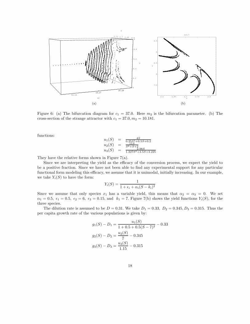
In a Neimark-Sacker bifurcation, both eigenvalues of the Poincare map cross the unit circle. The periodicorbit persists but changes its stability The stable limit cycle is replaced by a stable invariant torus thatmay have either rational or irrational rotation number. In either case, the species still coexist althoughthe corresponding orbit may no longer be periodic. Specifically, in case of an irrational rotation number,such an orbit will be dense on the invariant torus produced via the Neimark-Sacker bifurcation. Figure6(a) is a bifurcation diagram that shows one instance of the (supercritical) Neimark-Sacker bifurcation.This diagram was computed with c1 = 37.0, and it shows quite nicely how the stable periodic orbitis replaced by an invariant torus, and then the torus itself is replaced by a more complicated strangeattractor. Figure 6(b) shows a cross section of the strange attractor when the invariant torus loses itssmoothness and breaks up.

4.2 Yield included in the growth equation

In the following, we specialize system (13) to the case of three competing species and assume that xi

models the concentration of species i. We assume that ui(S) models the uptake of nutrient and that thegrowth term takes the form gi(S) = Yi(S)ui(S). One interpretation of the yield Yi(S) in this section isto model the efficacy of the conversion process and allow it to depend on the substrate concentration.

16

0.2

0.4

0.6

0.8

S

1

2

3

4

x

5

10

y

0.2

0.4

0.6

0.8

S

5

0

(a)

0.4

0.6

0.8

S

1

1.5

2

2.5

x

2

4

6

8

y

0.4

0.6

0.8

S

2

4

6

(b)

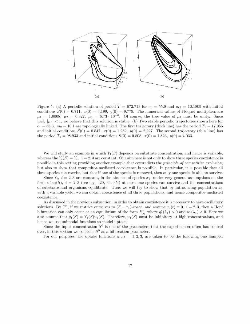
Figure 5: (a) A periodic solution of period T = 672.713 for c1 = 55.0 and m2 = 10.1809 with initialconditions S(0) = 0.711, x(0) = 3.199, y(0) = 9.779. The numerical values of Floquet multipliers areµ1 = 1.0008, µ2 = 0.827, µ3 = 6.73 · 10−6. Of course, the true value of µ1 must be unity. Since|µ2|, |µ3| < 1, we believe that this solution is stable. (b) Two stable periodic trajectories shown here forc1 = 38.3, m2 = 10.1 are topologically linked. The first trajectory (thick line) has the period T1 = 17.055and initial conditions S(0) = 0.547, x(0) = 1.282, y(0) = 2.227. The second trajectory (thin line) hasthe period T2 = 98.933 and initial conditions S(0) = 0.808, x(0) = 1.823, y(0) = 4.033.

We will study an example in which Y1(S) depends on substrate concentration, and hence is variable,whereas the Yi(S) = Yi, i = 2, 3 are constant. Our aim here is not only to show three species coexistence ispossible in this setting providing another example that contradicts the principle of competitive exclusion,but also to show that competitor-mediated coexistence is possible. In particular, it is possible that allthree species can coexist, but that if one of the species is removed, then only one species is able to survive.

Since Yi, i = 2, 3 are constant, in the absence of species x1, under very general assumptions on theform of ui(S), i = 2, 3 (see e.g. [20, 34, 35]) at most one species can survive and the concentrationsof substrate and organisms equilibrate. Thus we will try to show that by introducing population x1

with a variable yield, we can obtain coexistence of all three populations, and hence competitor-mediatedcoexistence.

As discussed in the previous subsection, in order to obtain coexistence it is necessary to have oscillatorysolutions. By (7), if we restrict ourselves to (S − x1)-space, and assume xi(t) ≡ 0, i = 2, 3, then a Hopfbifurcation can only occur at an equilibrium of the form E∗

λ1where g′1(λ1) > 0 and u′

1(λ1) < 0. Here wealso assume that g1(S) = Y1(S)u1(S). Therefore, u1(S) must be inhibitory at high concentrations, andhence we use unimodal functions to model uptake.

Since the input concentration S0 is one of the parameters that the experimenter often has controlover, in this section we consider S0 as a bifurcation parameter.

For our purposes, the uptake functions ui, i = 1, 2, 3, are taken to be the following one humped

17

10.1610.17

10.18

m2

2.62.652.72.75

x

8

8.2

8.4

8.6

8.8

9

y

10 1610.17

10.18

2.

(a)

2.6 2.65 2.7 2.75 2.8x

7.5

8

8.5

9

9.5

y

S=0.7

(b)

Figure 6: (a) The bifurcation diagram for c1 = 37.0. Here m2 is the bifurcation parameter. (b) Thecross-section of the strange attractor with c1 = 37.0, m2 = 10.181.

functions:u1(S) = 4S

0.25S2+0.5S+0.2

u2(S) = 11SS2+S+2

u3(S) = 2.98S1.227S2+3.5S+3.225

They have the relative forms shown in Figure 7(a).Since we are interpreting the yield as the efficacy of the conversion process, we expect the yield to

be a positive fraction. Since we have not been able to find any experimental support for any particularfunctional form modeling this efficacy, we assume that it is unimodal, initially increasing. In our example,we take Yi(S) to have the form:

Yi(S) =1

1 + εi + αi(S − ki)2

Since we assume that only species x1 has a variable yield, this means that α2 = α3 = 0. We setα1 = 0.5, ε1 = 0.5, ε2 = 6, ε3 = 0.15, and k1 = 7. Figure 7(b) shows the yield functions Yi(S), for thethree species.

The dilution rate is assumed to be D = 0.31. We take D1 = 0.33, D2 = 0.345, D3 = 0.315. Thus theper capita growth rate of the various populations is given by:

g1(S) − D1 =u1(S)

1 + 0.5 + 0.5(S − 7)2− 0.33

g2(S) − D2 =u2(S)

7− 0.345

g3(S) − D3 =u3(S)1.15

− 0.315

18

0 1 2 3 4 5 6 7 8 90

0.5

1

1.5

2

2.5

3

3.5

4

Substrate concentration

u j(S)

Species 1

Species 2

Species 3

(a)

0 1 2 3 4 5 6 7 8 9 100

0.1

0.2

0.3

0.4

0.5

0.6

0.7

0.8

0.9

Substrate concentration

1/(1

+ε1+

α 1 (S

−k 1)2 )

Species 3

Species 1

Species 2

(b)

1.5 2 2.5 3 3.5 4

−0.08

−0.06

−0.04

−0.02

0

0.02

0.04

0.06

0.08

0.1

0.12

Substrate concentration

g j(S)

− D

j

Species 1

Species 2

Species 3

(c)

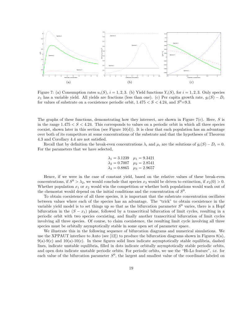
Figure 7: (a) Consumption rates ui(S), i = 1, 2, 3. (b) Yield functions Yi(S), for i = 1, 2, 3. Only speciesx1 has a variable yield. All yields are fractions (less than one). (c) Per capita growth rate, gi(S) − Di

for values of substrate on a coexistence periodic orbit, 1.475 < S < 4.24, and S0=9.3.

The graphs of these functions, demonstrating how they intersect, are shown in Figure 7(c). Here, S isin the range 1.475 < S < 4.24. This corresponds to values on a periodic orbit in which all three speciescoexist, shown later in this section (see Figure 10(d)). It is clear that each population has an advantageover both of its competitors at some concentrations of the substrate and that the hypotheses of Theorem4.3 and Corollary 4.4 are not satisfied.

Recall that by definition the break-even concentrations λi and µi are the solutions of gi(S)−Di = 0.For the parameters that we have selected,

λ1 = 3.1239 µ1 = 9.3421λ2 = 0.7007 µ2 = 2.8541λ3 = 0.8865 µ3 = 2.9657

Hence, if we were in the case of constant yield, based on the relative values of these break-evenconcentrations, if S0 > λ2, we would conclude that species x3 would be driven to extinction, if x2(0) > 0.Whether population x1 or x2 would win the competition or whether both populations would wash out ofthe chemostat would depend on the initial conditions and the concentration of S0.

To obtain coexistence of all three species, it is important that the substrate concentration oscillatesbetween values where each of the species has an advantage. The “trick” to obtain coexistence in thevariable yield model is to set things up so that as the bifurcation parameter S0 varies, there is a Hopfbifurcation in the (S − x1) plane, followed by a transcritical bifurcation of limit cycles, resulting in aperiodic orbit with two species coexisting, and finally another transcritical bifurcation of limit cyclesinvolving all three species. Of course, to claim coexistence, the resulting limit cycle involving all threespecies must be orbitally asymptotically stable in some open set of parameter space.

We illustrate this in the following sequence of bifurcation diagrams and numerical simulations. Weuse the XPPAUT interface to Auto (see [12]) to produce the bifurcation diagrams shown in Figures 8(a),9(a)-9(c) and 10(a)-10(c). In these figures solid lines indicate asymptotically stable equilibria, dashedlines, indicate unstable equilibria, filled in dots indicate orbitally asymptotically stable periodic orbits,and open dots indicate unstable periodic orbits. For periodic orbits, we use the “Hi-Lo feature”, i.e. foreach value of the bifurcation parameter S0, the largest and smallest value of the coordinate labeled on

19

(a) (b)

Figure 8: (a) Bifurcation diagram with stability with respect to (S − x1)-space only. This figure showstwo bifurcations: at S0 = 8.984, there is a subcritical Hopf bifurcation; at S0 = 8.833, a saddle node oflimit cycles. (b) Numerical simulation showing two periodic orbits in the (S − x1)-face when S0 = 8.92,as predicted by the bifurcation diagram. The inside one is unstable and the outside one is orbitallyasymptotically stable.

the ordinate axis is graphed.First we restrict our attention to the (S − x1)-face. Figure 8(a) shows two bifurcations with the

stability with respect to this face only. An analogous bifurcation diagram is shown in Figure 9(a) withthe stability given with respect to (S, x1, x2, x3)−space. This diagram was plotted with XPPAUT, andshows the minimal and maximal value of x1, along the periodic orbit, for different values of S0. There isa subcritical Hopf bifurcation at S0 = 8.984, and a saddle node of limit cycles at S0 = 8.833. Figure 8(b),shows two periodic orbits in the (S, x1)-face, for S0 = 8.92. There are two periodic orbits. The innerorbit is unstable and the outer one is asymptotically stable. The unstable orbit was plotted using reversedtime integration.

Figure 9 shows bifurcation curves for which x1 and x2 are nonnegative, but x3 = 0. In this figure thestability is given with respect to (S, x1, x2, x3)-space. Comparing Figure 8(a) with Figure 9(a), we seethat besides the Hopf bifurcation and the saddle node of limit cycles in the (S, x1)-face, there is a branchpoint at S0 = 8.899. The outer periodic orbit that is stable with respect to (S, x1)-space is unstablefor 8.833 < S0 < 8.899 with respect to (S, x1, x2, x3)-space. There is a transcritical bifurcation of limitcycles as S0 increases through the branch point S0 = 8.899, resulting in a branch of unstable periodicorbits with xi > 0, i = 1, 2. Along this branch, when S0 increases through 9.315 this branch stabilizesand the periodic orbits remain stable until S0 decreases through 9.155. Hence, there is stable coexistenceof species x1 and x2 for 9.155 < S0 < 9.315. Continuing along this branch, it stabilizes again as S0

decreases through 8.968 and remains stable until it collapses into the plane via a transcritical bifurcationat approximately 8.833. So there is also stable coexistence of x1 and x2 for 8.833 < S0 < 8.968. Anexample of this oscillatory coexistence of x1 and x2 is shown shown in Figure 9(d).

Figure 10 shows bifurcation curves for which xi ≥ 0, i = 1, 2, 3. There is a transcritical bifurcation of

20

0.3

0.4

0.5

0.6

0.7

0.8

0.9

1

1.1

1.2

X1

8.4 8.6 8.8 9 9.2 9.4 9.6 9.8S0

(a)

0

0.2

0.4

0.6

0.8

1

1.2

X1

8.4 8.6 8.8 9 9.2 9.4 9.6 9.8S0

(b)

0

0.1

0.2

0.3

0.4

0.5

0.6

X2

8.4 8.6 8.8 9 9.2 9.4 9.6 9.8S0

(c)

0.35

0.4

0.45

0.5

0.55

0.6

0.65

x1

0.085 0.09 0.095 0.1 0.105 0.11 0.115 0.12 0.125 0.13x2

(d)

Figure 9: (a)-(c) Bifurcation diagrams showing stability with respect to (S, x1, x2, x3)-space. (a) Bifur-cations in the (S, x1)-face. Besides the Hopf and saddle node bifurcations shown in Figure 8(a), thereis a branch point at S0 = 8.899. Only bifurcations with x1 > 0 and xi = 0, i = 2, 3 are shown. (b)and (c) Only bifurcation curves with species x1 and x2 nonnegative and x3 = 0 are shown. There isstable coexistence of species x1 and x2 for 8.833 < S0 < 8.968 and 9.155 < S0 < 9.315. (d) A numericalsimulation showing stable oscillatory coexistence of x1 and x2, for S0 = 8.92.

the limit cycle in the (S, x1, x2)-face (with x3 ≡ 0) into the positive cone. This branch of periodic orbitsremains stable until S0 increases through 9.479. Hence there is stable coexistence of all three species for8.965 < S0 < 9.479. Examples of such stable limit cycles, for different values of S0, are shown in Figure10(d).

Note that Figure 10(d) shows that at one of the boundaries of the coexistence state, S0 = 9.479, aNeimark-Sacker is detected, and hence more complex dynamics is likely for S0 > 9.479.

Finally, we note that this is an example of competitor-mediated coexistence. For 8.965 ≤ S0 ≤ 9.479,all three species coexist. However, x3 cannot survive in the presence of x2 unless x1 is also present.

21

0

0.2

0.4

0.6

0.8

1

1.2

X1

8.4 8.6 8.8 9 9.2 9.4 9.6 9.8S0

(a)

0

0.1

0.2

0.3

0.4

0.5

0.6

X2

8.4 8.6 8.8 9 9.2 9.4 9.6 9.8S0

(b)

(c)

0

0.25

0.5

0.75

1

1.250.242977

0.449003

0.65503

0.122162 0.147741 0.17332 0.198899 0.224478

x1

x2

x3

NS

BPC

NS

BPC

(d)

Figure 10: (a)-(c) Bifurcation diagrams showing branches where xi ≥ 0, i = 1, 2, 3. There is stablecoexistence of all three species for 8.965 < S0 < 9.479. (a) x1 on the ordinate axis, (b) x2 on the ordinateaxis, (c) x3 on the ordinate axis. (d) Three species stable oscillatory coexistence for a range of values8.965 < S0 < 9.479. This figure was done using CONTENT (see [17]). At S0 = 8.965, a branch point isdetected corresponding to a transcritical bifurcation of limit cycles, and at S0 = 9.479, a Neimark-Sackerbifurcation is detected.

5 Discussion

Clearly, the fact that the yield may vary with the nutrient concentration has profound implications forcoexistence of several microbial species. The principle of competitive exclusion states that at most onespecies can survive on a single nutrient at steady state. If one of the competitors exhibits a variable yield,then oscillatory coexistence of more than one species becomes possible.

We have presented one scenario in which the variable yield resulted in the coexistence of two species.Variable yield of the stronger competitor x was beneficial to the weaker competitor y. Specifically, wedemonstrated that if the stronger competitor x has a variable yield which generates a stable limit cyclein the plane y = 0, than the limit cycle can bifurcate into the coexistence region so that both x and ycan stably coexist in oscillatory fashion. Interestingly, a weaker competitor can also benefit if its ownyield is variable. If x is a weaker competitor than y at steady state and x exhibits variable yield, then it

22

is possible that both the steady state with x = 0 and the limit cycle with y = 0 are stable and thereforethe outcome of competition will depend on the initial conditions. This is a clear benefit to the weakercompetitor x because it enables x to outcompete y for some open nonempty set of initial conditions. Thesecond scenario corresponds to bistability.

We also demonstrated that three species coexistence in this context is possible and that competitor-mediated coexistence can occur. In this case, two competitors x2 and x3 with fixed yields, a situationthat would normally lead to competitive exclusion, are lead to coexistence by the intervention of a thirdcompetitor with variable yield, x1. The latter acts as a mediator, causing oscillations in the substratedensity that make the value of S alternatively beneficial for x2 and x3.

In addition to facilitating oscillatory coexistence, the model with variable yield can display muchmore complicated dynamics. We have presented several examples of dynamically nontrivial attractorscorresponding to coexistence (long periodic orbits, invariant tori, linked stable periodic orbits). In aspecial limiting case, model (15) can exhibit intermittent trajectories if the break-even concentrations ofx and y are sufficiently close.

We also explained why it is important to understand how the yield depends on the substrate inorder to incorporate the term correctly in the model. In any model in which the yield is considered ameasure of the efficacy of the conversion process, the growth and uptake terms are related by the equationg(S) = Y (S)u(S). In order for such a single species growth model to exhibit a Hopf bifurcation, theuptake rate u(S) must be decreasing at high substrate concentrations. In formulating such a model, onetherefore must assume that uptake of the substrate is inhibited by high concentrations of substrate. Thisobservation may prove important if one is actually going to try to find organisms in order to observe thisphenomenon in the laboratory.

References[1] P. Agrawal, C. Lee, H. C. Lim, and D. Ramkrishna. Theoretical investigations of dynamic behavior of

isothermal continuous stirred tank biological reactors. Chemical Engineering Science, 37(3):453–462,1982.

[2] J. F. Andrews. A mathematical model for the continuous culture of microorganisms utilizing in-hibitory substrates. Biotechnology and Bioengineering, 10:707–723, 1968.

[3] G. E. Briggs and J. B. S. Haldane. A note on the kinetics of enzyme action. Biochem. J., 19:338–339,1925.

[4] G. J. Butler and P. Waltman. Bifurcation from a limit cycle in a two predator-one prey ecosystemmodeled on a chemostat. J. Math. Biol., 12:295–310, 1981.

[5] G. J. Butler and G.S.K. Wolkowicz. A mathematical model of the chemostat with a general class offunctions describing nutrient uptake. SIAM J. Appl. Math., 45(1):138–151, 1985.

[6] P. H. Calcott, editor. Continuous Cultures of Cells. CRC Press, 1981.[7] P. Crooke and R. Tanner. Hopf bifurcations for a variable yield continuous fermentation model. Int.

J. Engng. Sci., 20(3):439–443, 1982.[8] P. Crooke, C.-J. Wei, and R. Tanner. The effect of the specific growth rate and yield expressions

on the existence of oscillatory behavior of a continuous fermentation model. Chem. Eng. Commun.,6:333–347, 1980.

[9] G. Dinopoulou, R. M. Sterritt, and J. N. Lester. Anaerobic acidogenesis of a complex wastewater: II.kinetics of growth, inhibition, and product formation. Biotechnology and Bioengineering, 31:969–978,1988.

[10] A. G. Dorofeev, M. V. Glagolev, T. F. Bondarenko, and N. S. Panikov. Observation and explanationof the unusual growth kinetics of Arthrobacter globiformis. Microbiology, 61:24–31, 1992.

23

[11] V. H. Edwards. The influence of high substrate concentrations on microbial kinetics. Biotechnologyand Bioengineering, 12:679–712, 1970.

[12] B. Ermentrout, editor. Simulating, Analyzing, and Animating Dynamical Systems: A guide toXPPAUT for researhers and students. SIAM, Philadelphia, 2002.

[13] C. K. Essajee and R. D. Tanner. The effect of extracellular variables on the stability of the continuousbaker’s yeast-ethanol fermentation process. Process Biochemistry, 1979.

[14] F. B. Godin, D. G. Cooper, and A. D. Rey. Development and solution of a cell mass populationbalance model applied to the scf process. Chemical Engineering Science, 54:565–578, 1999.

[15] S. B. Hsu. Limiting behavior for competing species. SIAM J. Appl. Math., 34:760–763, 1978.[16] S. Koga and A. E. Humphrey. Study of the dynamic behavior of the chemostat system. Biotechnology

and Bioengineering, 9:375–386, 1967.[17] Y. A. Kuznetsov, editor. CONTENT - Integrated Environment for Analysis of Dynamical Systems.

Report, UPMA-98-224, Ecole Normale Superioure de Lyon, Lyon, France, 1998.[18] I. H. Lee, A. G. Fredrickson, and H. M. Tsuchiya. Damped oscillations in continuous culture of

Lactobacillus plantarum. Journal of General Microbiology, 93:204–208, 1976.[19] Y. Lenbury, P. S. Crooke, and R. D. Tanner. Relating damped oscillations to sustained limit cycles

describing real and ideal batch fermentation processes. BioSystems, 19:15–22, 1986.[20] B. Li. Global asymptotic behavior of the chemostat: general response functions and differential

death rates. SIAM J. Appl. Math., 59:411–422, 1999.[21] J. E. Littlewood. A mathematician’s miscellany. Methuen and Co., London, 1953.[22] J. H. T. Luong. Generalization of Monod kinetics for analysis of growth data with substrate inhibi-

tion. Biotechnology and Bioengineering, 29:242–248, 1987.[23] J. E. Marsden and M. McCracken. The Hopf Bifurcation and its Applications. Springer, 1976.[24] J. Monod. The growth of bacterial cultures. Annual Review of Microbiology, 3:371–394, 1949.[25] A. Moser. Bioprocess Technology. Springer, 1988.[26] S. S. Pilyugin and P. Waltman. Divergence criterion for generic planar systems. SIAM J. Appl.

Math., 64(1):81–93, 2003.[27] S. S. Pilyugin and P. Waltman. Multiple limit cycles in the chemostat with variable yield. Math.

Biosciences, 182:151–166, 2003.[28] N. S. Rao and E. O. Roxin. Controlled growth of competing species. SIAM J. Appl. Math., 50(3):853–

864, 1990.[29] S. C. Ricke and D. M. Schaefer. Growth and fermentation responses of Selenomonas ruminantium to

limiting and non-limiting concentrations of amonium chloride. Appl. Microbiol. Biotechnol., 46:169–175, 1996.

[30] H. L. Smith and P. Waltman. The theory of the chemostat. Cambridge University Press, 1995.[31] J. M. VanBriesen. Evaluation of methods to predict bacterial yield using thermodynamics. Biodegra-

dation, 13:171–190, 2002.[32] J. L. Webb. Enzyme and Metabolic Inhibitors. Volume I. General Principles of Inhibition. Academic

Press, 1963.[33] G. S. K. Wolkowicz. Bifurcation analysis of a predator-prey system involving group defense. SIAM

J. Appl. Math., 48(3):592–606, 1988.[34] G. S. K. Wolkowicz and Z. Lu. Global dynamics of a mathematical model of competition in the

chemostat: general response functions and differential death rates. SIAM J. Appl. Math., 52(1):222–233, 1992.

[35] G. S. K. Wolkowicz and H. Xia. Global asymptotic behavior of a chemostat model with discretedelays. SIAM J. Appl. Math., 57(4):1019–1043, 1997.

24

A APPENDIX – Proof of Theorem 2.6

Equation (8) is the transversality condition.Let ω0 =

√x∗u(S∗)g′(S∗), denote the imaginary part of the eigenvalue at the critical value αc, of the Hopf

bifurcation parameter. Take

T =

[0 −1

ω0u(S∗)

0

]and T−1 =

[0 u(S∗)

ω0−1 0

]

(rv

)= T−1

(Sx

)⇒

r = x u(S∗)

ω0

v = −S

Thus, in canonical form the system is

dr

dt= r(−D1 + g(−v)) ≡ f(r, v)

dv

dt= −(S0 + v)D + r

ω0

u(S∗)u(−v) ≡ g(r, v)

Now the system is in the canonical form so that a straight forward application of the formula in Marsden andMcCracken [23] shows that the sign of CH determines the criticality of the Hopf bifurcation as indicated inTheorem 2.6.

Alternatively, defining h(s) = D(S0−S)u(S)

, one can write the system (1) in the form:

dS

dt= (

D(S0 − S)

u(S)− x)u(S) ≡ (h(S) − x)u(S)

dx

dt= (g(S) − D1)x.

In [33] the criterion for the criticality of the Hopf bifurcation based on the sign of CH was derived.

25