conet mobile lab - agh university of science and...

CoNeT Mobile Lab Ethernet IP – module 5

- Instructions for the practical exercises – Revision 1.0

Co-operative Network Training AGH University of Science and Technology Department of Automatics http://www.ia.agh.edu.pl Contact: [email protected]

Content 3

Content

Content ........................................... ........................................................................... 3

1 Configuring the network ........................... ......................................................... 5

1.1 CREATING A NEW PROJECT AND CONFIGURING THE ETHERNET/IP NODES IN RSLOGIX5000 .................. 7 1.2 CONFIGURING THE ETHERNET/IP NODES .............................................................................................. 11

1.3 ADDRESS I/O DATA OF CONFIGURED MODULES..................................................................................... 19

2 Analysing and understanding PLC functionality ..... ...................................... 25

2.1 INTRODUCTION ..................................................................................................................................... 25

2.2 UNDERSTANDING THE CONET_BASE PROJECT..................................................................................... 25

2.3 RUNNING THE APPLICATION. ................................................................................................................. 35

3 Analysing and understanding other components ...... ................................... 37

3.1 INVERTER POWERFLEX 40 .................................................................................................................... 37 3.1.1 Configuration of the PowerFlex40 ................................................................................................ 37 3.1.2 Detailed configuration of the PowerFlex40 .................................................................................. 39

3.2 HMI (HUMAN MACHINE INTERFACE) PANELV IEW PLUS 600 ............................................................... 51 3.3 BIBLIOGRAPHY ..................................................................................................................................... 61

4 Monitoring of the Ethernet/IP network traffic ..... ............................................ 63

4.1 EXERCISE 1. .......................................................................................................................................... 71

4.2 EXERCISE 2. .......................................................................................................................................... 73

4 . Content

1. Configuring the network

5

1 Configuring the network

RSLinx Classic for Rockwell Automation Networks and Devices is a compre-hensive factory communications solution for use with the Microsoft Windows operating systems. It is mainly used to configure the network parameters, DDE OPC servers and to program and communicate with PLC controllers. Th RSLinx Classic cooperates with all Rockwell Automation programming and configuration applications such as RSLogix, RSNetWorx, RSView32 (HMI), FactoryTalk View SE, and FactoryTalk View ME Station. It’s also possible to build your own data monitoring and acquisition applications using third party application: MATLAB/Simulink, LabView, Microsoft Office etc. RSLinx Classic also incorporates advanced data optimization techniques and contains a set of diagnostics. This section outlines the main tasks you will need to configure and test the Ethernet/IP network using the RSLinx Classic software. The table 1 contains the information necessary to correctly configure the network nodes. Table 1: Ethernet/IP parameters of the laboratory setup modules

CompactLogix

L35E 1734-AENT PanelView Plus 600 PowerFlex40 WAGO 750-341

IP Address 192.168.1.1 192.168.1.2 192.168.1.3 192.168.1.5 192.168.1.182

Subnet Mask 255.255.255.0 255.255.255.0 255.255.255.0 255.255.255.0 255.255.255.0

Gateway IP Address

none none none none none

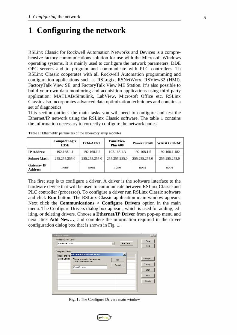
The first step is to configure a driver. A driver is the software interface to the hardware device that will be used to communicate between RSLinx Classic and PLC controller (processor). To configure a driver run RSLinx Classic software and click Run button. The RSLinx Classic application main window appears. Next click the Communications > Configure Drivers option in the main menu. The Configure Drivers dialog box appears, which is used for adding, ed-iting, or deleting drivers. Choose a Ethernet/IP Driver from pop-up menu and next click Add New…, and complete the information required in the driver configuration dialog box that is shown in Fig. 1.

Fig. 1: The Configure Drivers main window


6

1. Configuring the network 7

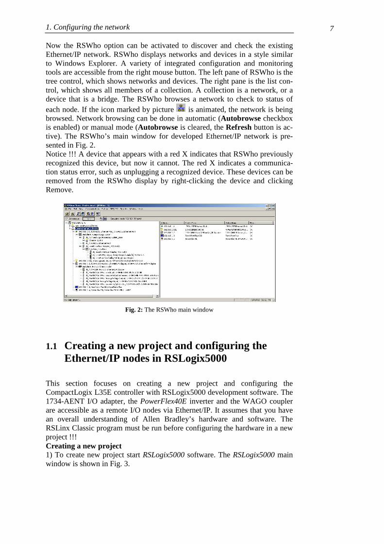
Now the RSWho option can be activated to discover and check the existing Ethernet/IP network. RSWho displays networks and devices in a style similar to Windows Explorer. A variety of integrated configuration and monitoring tools are accessible from the right mouse button. The left pane of RSWho is the tree control, which shows networks and devices. The right pane is the list con-trol, which shows all members of a collection. A collection is a network, or a device that is a bridge. The RSWho browses a network to check to status of each node. If the icon marked by picture is animated, the network is being browsed. Network browsing can be done in automatic (Autobrowse checkbox is enabled) or manual mode (Autobrowse is cleared, the Refresh button is ac-tive). The RSWho’s main window for developed Ethernet/IP network is pre-sented in Fig. 2. Notice !!! A device that appears with a red X indicates that RSWho previously recognized this device, but now it cannot. The red X indicates a communica-tion status error, such as unplugging a recognized device. These devices can be removed from the RSWho display by right-clicking the device and clicking Remove.

Fig. 2: The RSWho main window

1.1 Creating a new project and configuring the Ethernet/IP nodes in RSLogix5000

This section focuses on creating a new project and configuring the CompactLogix L35E controller with RSLogix5000 development software. The 1734-AENT I/O adapter, the PowerFlex40E inverter and the WAGO coupler are accessible as a remote I/O nodes via Ethernet/IP. It assumes that you have an overall understanding of Allen Bradley’s hardware and software. The RSLinx Classic program must be run before configuring the hardware in a new project !!! Creating a new project 1) To create new project start RSLogix5000 software. The RSLogix5000 main window is shown in Fig. 3.


8


Fig. 3: The RSLogix5000 new project main window

2) Create a new project by select the New Project item (or the File\New menu item). The New Controller dialog window is displayed (see Fig. 4). The fol-lowing parameters must be set:

• Type:1769-L35E CompactLogix5335E Controller • Revision:16 • Name:Enter an appropriate name (here CoNet_Base) • Description:Enter an appropriate description • Chassis Type:<none> • Slot:0 • Created In:Enter an appropriate folder

Fig. 4: The New Controller dialog window


10


3) Press the OK button 4) Open the I/O Configuration folder in the project window tree. Expand the tree and find CompactBusLocal item. Right click on CompactBusLocal and select the New Module… menu item. The Select Module window is dis-played. 5) Select 1769-IQ6XOW4/B from the list and click OK . 6) The Module Properties dialog window is displayed. 7) Enter the following parameters:

• Name:Local_DIO, • Slot:1 (slot of the scanner).

8) Repeat steps 4-7 for 1769-IF4XOF2/A module. The module properties are: • Name:Local_AIO, • Slot:2.

9) Select the Communications -> Download program menu item. After down-loading, if everything was setup correctly, the “I/O OK” indicator is green.

1.2 Configuring the Ethernet/IP nodes

The proposed network structure contains at least four nodes: CompactLogix L35E controller, 1734-AENT POINT-IO, PowerFlex 40 inverter and WAGO I/O adapter. The CompactLogix L35E controller is a local one and it is config-ured when a new project is created. The all others are a distributed nodes and must be separately added to project. 1734-AENT POINT-IO 1) Open the I/O Configuration folder in the project window tree. Expand the tree and find 1769-L35E Ethernet Port LocalENB item. Right click on Ethernet and select the New Module… menu item. The Select Module win-dow is displayed. 2) Select 1734-AENT/A from the list and click OK . 3) The Module Properties dialog window is displayed (see Fig. 5). 4) Choose the General tag and enter the following parameters:

• Name:Distributed_IO, • IP Address:192.168.1.2, • Chassis Size:6, • Revision:2.3, • Electronic Keying:Compatible Keying.


12


Fig. 5: Module properties of 1734-AENT/A Ethernet Adapter

5) Select the Connection tag and set the Requested Packed Interval (RPI) to 100.0 ms (Fig. 6). This parameter decides about refreshing of I/O data over the Ethernet/IP network.

Fig. 6: Connection tap of module properties

Notice !!! The RPI is common parameter configuring for the all modules con-nected to a network. It specifies the period at which data updates over a con-nection. For example, an input module sends data to a controller at the RPI that is assigned to the module. Typically an RPI is configured in milliseconds (ms). The range is 0.2 ms to 750 ms. If a Ethernet/IP network connects the devices, the RPI reserves a slot in the stream of data flowing across the network. The timing of this slot may not coincide with the exact value of the RPI, but the control system guarantees that the data transfers at least as often as the RPI. 6) Press OK button. The new 1734-AENT/A Distributed_IO item and PointIO 6 Slot Chassis sub-item in the project tree are displayed. 7) Right click on PointIO 6 Slot Chassis and select the New Module… menu item. The Select Module window is displayed. 8) Select 1734-IB8 from the list and click OK . 9) The Module Properties dialog window is displayed (see Fig. 7).


14


10) Choose the General tag and enter the following parameters: • Name:Remote_DI8, • Slot:1, • Revision:3.1.

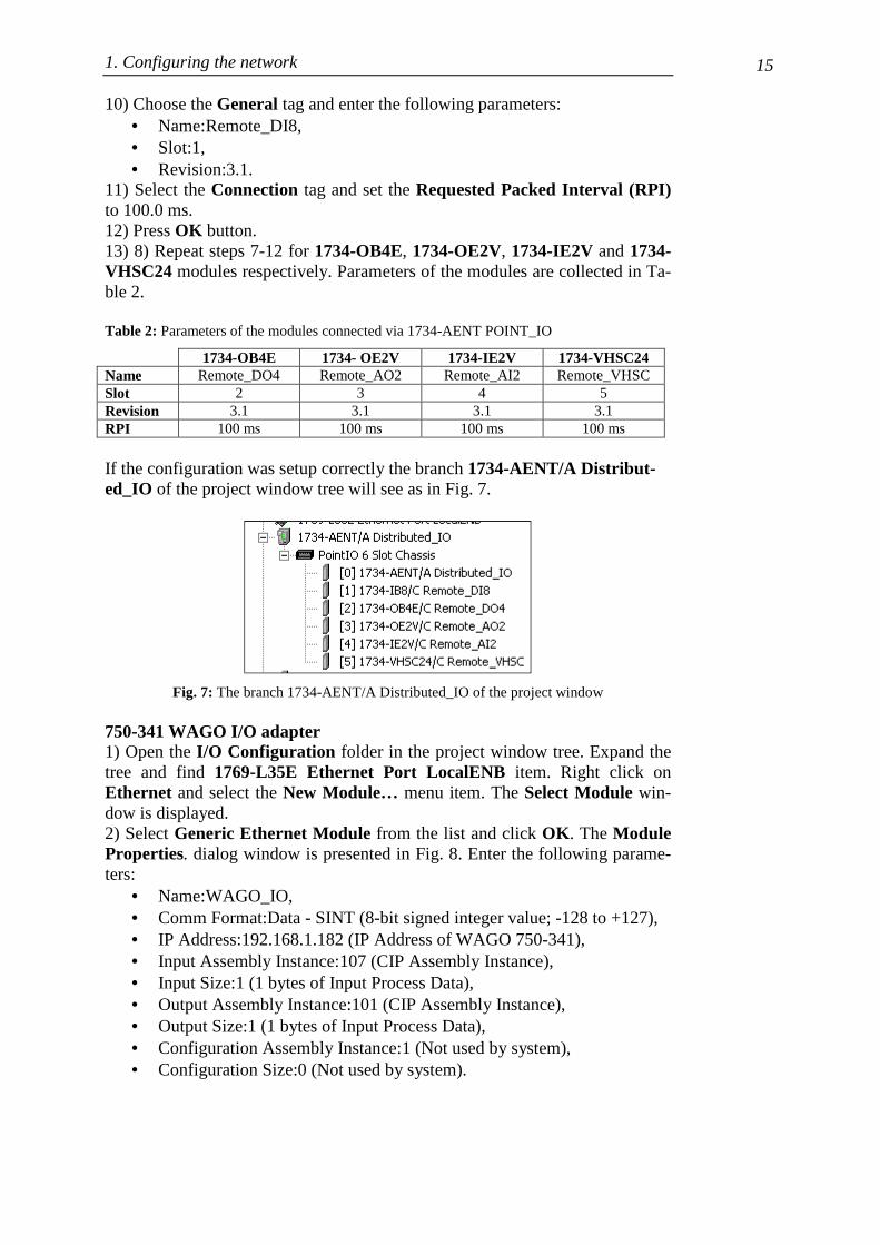
11) Select the Connection tag and set the Requested Packed Interval (RPI) to 100.0 ms. 12) Press OK button. 13) 8) Repeat steps 7-12 for 1734-OB4E, 1734-OE2V, 1734-IE2V and 1734-VHSC24 modules respectively. Parameters of the modules are collected in Ta-ble 2. Table 2: Parameters of the modules connected via 1734-AENT POINT_IO

1734-OB4E 1734- OE2V 1734-IE2V 1734-VHSC24 Name Remote_DO4 Remote_AO2 Remote_AI2 Remote_VHSC Slot 2 3 4 5 Revision 3.1 3.1 3.1 3.1 RPI 100 ms 100 ms 100 ms 100 ms If the configuration was setup correctly the branch 1734-AENT/A Distribut-ed_IO of the project window tree will see as in Fig. 7.

Fig. 7: The branch 1734-AENT/A Distributed_IO of the project window

750-341 WAGO I/O adapter 1) Open the I/O Configuration folder in the project window tree. Expand the tree and find 1769-L35E Ethernet Port LocalENB item. Right click on Ethernet and select the New Module… menu item. The Select Module win-dow is displayed. 2) Select Generic Ethernet Module from the list and click OK . The Module Properties. dialog window is presented in Fig. 8. Enter the following parame-ters:

• Name:WAGO_IO, • Comm Format:Data - SINT (8-bit signed integer value; -128 to +127), • IP Address:192.168.1.182 (IP Address of WAGO 750-341), • Input Assembly Instance:107 (CIP Assembly Instance), • Input Size:1 (1 bytes of Input Process Data), • Output Assembly Instance:101 (CIP Assembly Instance), • Output Size:1 (1 bytes of Input Process Data), • Configuration Assembly Instance:1 (Not used by system), • Configuration Size:0 (Not used by system).


16


The EtherNet/IP settings for the WAGO 750-341 are configured through the built-in web pages. Using a web browser like Microsoft Internet Explorer, Mozilla Firefox etc. The following parameters were set:

• The IP address: 192.168.1.182, • The EtherNet/IP protocol. Both the Modbus/TCP and Modbus/UDP

protocols must be disabled in order to map the input and output process image to an EtherNet/IP fieldbus master.

Fig. 8: Module properties of the WAGO I/O Adapter

PowerFlex 40E inverter 1) Open the I/O Configuration folder in the project window tree. Expand the tree and find 1769-L35E Ethernet Port LocalENB item. Right click on Ethernet and select the New Module… menu item. The Select Module win-dow is displayed. 2) Select PowerFlex 40-E from the list and click OK . The Module Proper-ties. dialog window is presented in Fig. 9. Enter the following parameters:

• Name:PowerFlex, • IP Address:192.168.1.5, • Revision:3.3.

Fig. 9: Properties of the PowerFlex 40E inverter


18


3) Press OK button. The item PowerFlex 40E PowerFlex will be added to the project tree. If the configuration of all nodes in the network is done correctly, the RSLogix 5000 main window should look like in the Fig. 10.

Fig. 10: The main window of RSLogix5000 project

The program/configuration can now be downloaded to the CompactLogix con-troller. Select the Communications -> Download program menu item. After downloading, if everything was setup correctly, the “I/O OK” indicator is green. If an error does occur, the improper connection size and/or communica-tion format was entered for either the input or output parameters.

1.3 Address I/O data of configured modules

The all I/O modules information is presented as a set of tags. Each tag uses a structure of data. The structure depends on the specific features of the I/O module. The name of the tags is based on the location of the I/O module in the system. An I/O address follows a format shown in Fig. 11.

Fig. 11: Address format of tags


20


LocationLOCAL = local chassis of the controller.

ADAPTER_NAME = identifies remote communication adapter or bridge module.

:SlotSlot number of I/O module in its chassis. :TypeType of data (I = input, O = output, C = configuration, S = status). .Member Specific data from the I/O module; depends on what type of data

the module can store. For a digital module, a Data member usu-ally stores the input or output bit values. For an analog module, a Channel member (CH#) usually stores the data for a channel.

.SubMember Specific data related to a Member.

.Bit Specific point on a digital I/O module; depends on the size of the I/O module.

The relationship between I/O configuration and the tag address is shown in Fig. 12. To expand a structure and display its members, click the „+” sign.

Fig. 12: Connection between I/O Configuration tree and the tag address

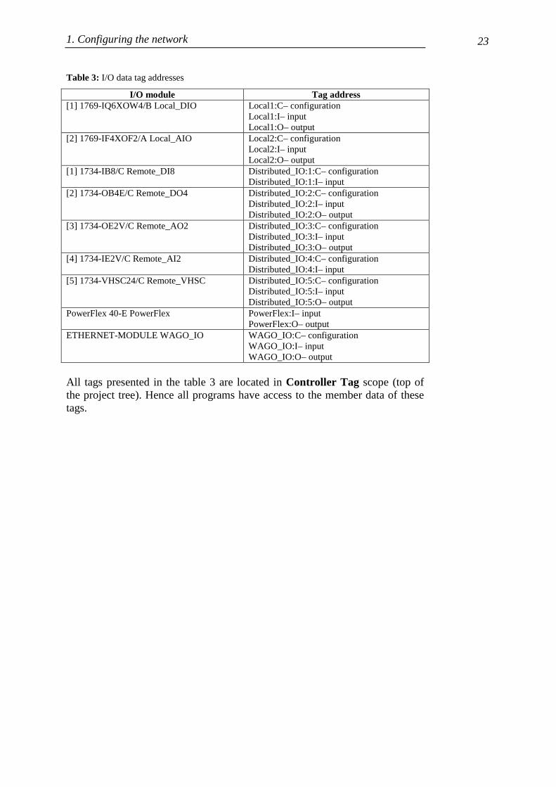
Table 3 lists the all configured I/O modules and corresponding tag addresses.


22


Table 3: I/O data tag addresses

I/O module Tag address [1] 1769-IQ6XOW4/B Local_DIO Local1:C– configuration

Local1:I– input Local1:O– output

[2] 1769-IF4XOF2/A Local_AIO Local2:C– configuration Local2:I– input Local2:O– output

[1] 1734-IB8/C Remote_DI8 Distributed_IO:1:C– configuration Distributed_IO:1:I– input

[2] 1734-OB4E/C Remote_DO4 Distributed_IO:2:C– configuration Distributed_IO:2:I– input Distributed_IO:2:O– output

[3] 1734-OE2V/C Remote_AO2 Distributed_IO:3:C– configuration Distributed_IO:3:I– input Distributed_IO:3:O– output

[4] 1734-IE2V/C Remote_AI2 Distributed_IO:4:C– configuration Distributed_IO:4:I– input

[5] 1734-VHSC24/C Remote_VHSC Distributed_IO:5:C– configuration Distributed_IO:5:I– input Distributed_IO:5:O– output

PowerFlex 40-E PowerFlex PowerFlex:I– input PowerFlex:O– output

ETHERNET-MODULE WAGO_IO WAGO_IO:C– configuration WAGO_IO:I– input WAGO_IO:O– output

All tags presented in the table 3 are located in Controller Tag scope (top of the project tree). Hence all programs have access to the member data of these tags.


24

2. Analysing and understanding PLC functionality 25

2 Analysing and understanding PLC functionality

2.1 Introduction

The main part of the Allen-Bradley demo case is the Compact Logix Controller 1769-L35E. The 1769-L35E controller is designed for mid-range applications. It is equipped in the operat-ing system with a pre-emptive multitasking system. This environment supports as many as 8 tasks, but only one can be continuous. A task can have as many as 32 separate programs with their own executable routines and program tags.

2.2 Understanding the CoNET_Base project

The CompactLogix 1769-L35E controller supports development programs in four languages: • Ladder Diagram

• Sequential Function Chart

• Function Block Diagram

• Structured Text

The main features of PLC programming are: − tasks: max. 8 tasks (only one can be continuous)

− programs: max. 32 separate programs in one task with its own routines and program-

scoped tags

− routines

Tasks – max. 8 tasks (only one can be continuous); all programs assigned to the task execute in the order in which they are grouped; each task has a priority level – from lowest priority of 15 up to the highest priority of 1; the continuous task has the lowest priority. Programs – max. 32 separate programs in one task; a program contains program tags, a main executable routine and other routines Routines – a set of logic instructions in a single programming language (e.g. ladder logic)

2. Analysing and understanding PLC functionality

26


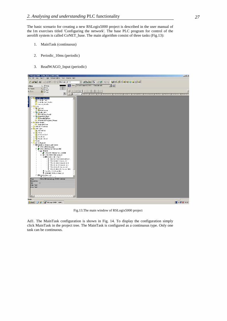
The basic scenario for creating a new RSLogix5000 project is described in the user manual of the 1m exercises titled 'Configuring the network'. The base PLC program for control of the aerolift system is called CoNET_base. The main algorithm consist of three tasks (Fig.13):

1. MainTask (continuous)

2. Periodic_10ms (periodic)

3. ReadWAGO_Input (periodic)

Ad1. The MainTask configuration is shown in Fig. 14. To display the configuration simply click MainTask in the project tree. The MainTask is configured as a continuous type. Only one task can be continuous.

Fig.13.The main window of RSLogix5000 project


28


In the section Program Tags you can define the local tags to be used in MainRoutine. MainRoutine contains a main PLC program which is written in ladder diagram (Fig. 15).

The program allows you to start and stop the PowerFlex inverter. For starting you should turn on the switch marked Local1:I.Data.0 – this means: bit 0 from Digital Input from digital

module in PLC (1769-L35E). To stop – turn on the switch marked Distributed_IO:1:I.0 – this means: bit 0 from Digital Input of the Distributed_IO module (1734-AENT).

Fig. 15. The ladder diagram in MainRoutine

Fig. 14.The parameters of the MainTask


30


Ad2. The Periodic_10ms task configuration is shown in Fig. 16. This task is configured as Pe-riodic with 100ms period. In this task program WriteFreq_Flex40 is defined.

The program allows control of the inverter frequency. Voltage from the adjuster on the panel is read by an analog input, processed and served as a control signal to the inverter. A detailed program in a ladder diagram is shown in Fig. 5. The digital input Local1:I.Data.1 is defined as ALW_ON tag in the WriteFreq_Flex40->ProgramTags section. The variables: AnalogIn1, FREQ and ControlFREQ are also defined in this section (Fig. 17). Variables are used to calcu-late a control frequency to the inverter.

Fig. 17. The variables of WriteFreq_Flex40->ProgramTags

Fig. 16. The parameters of the Periodic_10ms task


32


Ad3. The ReadWAGO_Input task configuration is shown in Fig. 20. The task is configured as Periodic with 25ms period. In this task program ReadProximitySensors is defined. The pro-gram is very simple – signals from digital inputs are read and moved to the variable SensorInput, which is defined in the ReadDigitalInput->ProgramTags section (Fig. 19).

Fig. 19. The variables of ReadDigitalInput->ProgramTags

Fig. 18.The WriteFreq program


34


2.3 Running the application.

To run the prepared program, first you should download it to the PLC. To do this first you can go online and next download (Fig. 21). The project will be automatically checked, loaded and start running. In on-line mode you can monitor all current process values.

Fig. 21. The 'Go Online' context menu

Fig.20. The parameters of ReadWAGO_Input task


36

3. Analysing and understanding other components 37

3 Analysing and understanding other components

3.1 Inverter PowerFlex 40

The Allen-Bradley PowerFlex 40 AC drive is the smallest and most cost-effective member of the PowerFlex family of drives. The PowerFlex 40 is designed to be used for speed control in applications such as machine tools, fans, pumps and conveyors and material handling systems. The main features of the PowerFlex40 AC drive are:

• integral keypad for simple operation and programming,

• 4 digit display with 10 LED indicators for display of drive status,

• communication with PC using the RS-485 interface, Ethernet/IP (also DeviceNet,

PROFIBUS DP, LonWorks and ControlNet interface are available),

• Autotune allows the user to take into account individual motor characteristics,

• Sensorless Vector Control provides exceptional speed regulation and very high

levels of torque across the entire speed range of the drive,

• built-in PID controller

• Timer, Counter, Basic Logic and StepLogic functions

• built-in digital and analog I/O (2 analog inputs, 7 digital inputs (4 fully

programmable), 1 analog output, 3 digital output)

• easy set-up over the network (RS NetWorx property)

3.1.1 Configuration of the PowerFlex40

Configuration of the PowerFlex40 AC drive requires a correctly prepared RSLogix500 project. Adding the PowerFlex40 as a new module to an existing project is done in the following way:

• Open the I/O Configuration folder in the existing RSLogix500 project. Expand the

folder tree and find the 1769-L35 Ethernet Port LocalENB item. Click the right

mouse button on the Ethernet item to activate the context menu and select New

Module....

3. Analysing and understanding other components

38


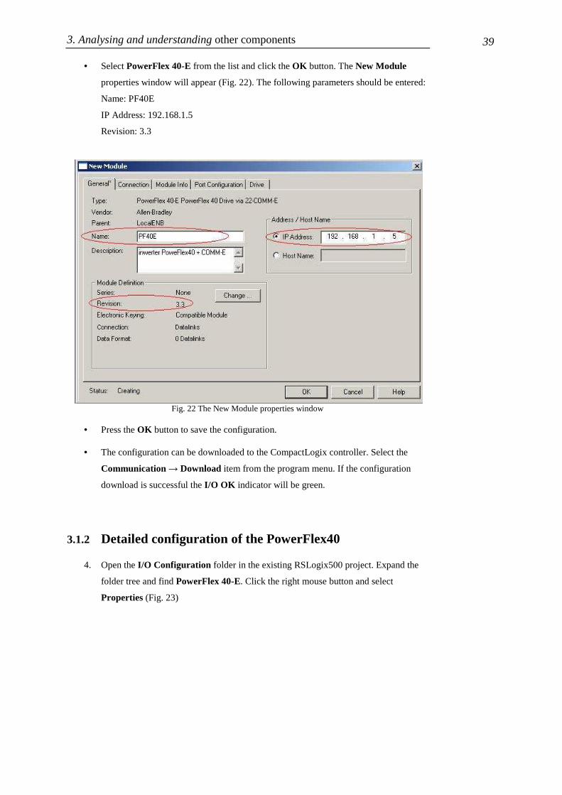
• Select PowerFlex 40-E from the list and click the OK button. The New Module

properties window will appear (Fig. 22). The following parameters should be entered:

Name: PF40E

IP Address: 192.168.1.5

Revision: 3.3

• Press the OK button to save the configuration.

• The configuration can be downloaded to the CompactLogix controller. Select the

Communication → Download item from the program menu. If the configuration

download is successful the I/O OK indicator will be green.

3.1.2 Detailed configuration of the PowerFlex40

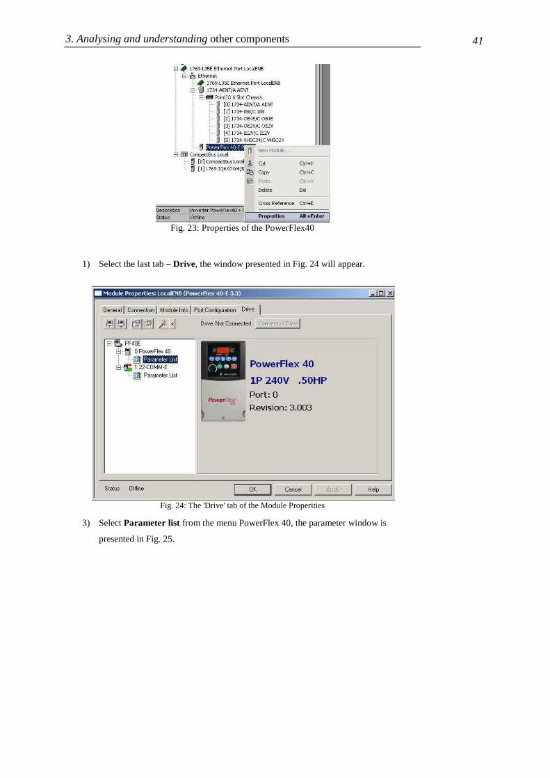
4. Open the I/O Configuration folder in the existing RSLogix500 project. Expand the

folder tree and find PowerFlex 40-E. Click the right mouse button and select

Properties (Fig. 23)

Fig. 22 The New Module properties window


40


1) Select the last tab – Drive, the window presented in Fig. 24 will appear.

3) Select Parameter list from the menu PowerFlex 40, the parameter window is

presented in Fig. 25.

Fig. 24: The 'Drive' tab of the Module Properities

Fig. 23: Properties of the PowerFlex40


42


Only the parameters on a white background can be changed. The selected parameters are shown in Table.4. Detailed descriptions of all parameters are included in [1].

Table 4:

ID Name of parameter Description

31 31 Motor NP Volts Set to the motor nameplate rated volts.

32 32 Motor NP Hertz Set to the motor nameplate rated frequency.

33 33 Motor OL Current Set to the maximum allowable motor current.

34 34 Minimum Freq Sets the lowest frequency the drive will output continuously.

35 35 Maximum Freq Sets the highest frequency the drive will output.

36 36 Start Source Sets the control scheme used to start the drive.

37 37 Stop Mode Active stop mode for all stop sources

Fig. 25. The Parameter List window.


44


38 38 Speed reference Sets the source of the speed reference to the drive.

39 39 Accel Time 1 Sets the rate of acceleration for all speed increases.

40 40 Decel Time 1 Sets the rate of deceleration for all speed decreases.

41 Reset To Defalts Resets all parameter values to factory defaults.

43 Motor OL Ret Enables/disables the Motor Overload Retention function.

51 Digital In1 Sel (I/O Terminal 05) Selects the function for the digital inputs.




55 Relay Out Sel Sets the condition that changes the state of the output relay contacts.

56 Relay Out Level Sets the trip point for the digital output relay if the value of 55 [Relay Out Sel] is 6, 7, 8, 10, 16, 17, 18 or 20.

58 61

Opto Out1 Sel Opto Out2 Sel

Determines the operation of the programmable opto outputs.

59 62

Opto Out1 Level Opto Out2 Level

Determines the on/off point for the opto outputs when 58 or 61 [Opto Outx Sel] is set to option 6, 7, 8, 10, 16, 17, 18 or 20.

64 Opto Out Logic Determines the logic (Normally Open/NO or Normally Closed/NC) of the opto outputs.

65 Analog Out Sel Sets the analog output signal mode (0-10V, 0-20mA, or 4-20mA).

66 Analog Out High Scales the Maximum Output Value for the 65 [Analog Out Sel] source setting.

67 Accel Time 2 When active, sets the rate of acceleration for all speed increases except jog.

68 Decel Time 2 When active, sets the rate of deceleration for all speed decreases ex-cept jog.

69 Internal Freq Provides the frequency command to the drive when 38 [Speed Refer-ence] is set to 1 “Internal Freq”.

70 71 72 73 74 75 76 77

Preset Freq 0 Preset Freq 1 Preset Freq 2 Preset Freq 3 Preset Freq 4 Preset Freq 5 Preset Freq 6 Preset Freq 7

Provides a fixed frequency command value when 51-53 [Digital Inx Sel] is set to 4 “Preset Frequencies”.

78 Jog Frequency Sets the output frequency when a jog command is issued.

79 Jog Accel/Decel Sets the acceleration and deceleration time when a jog command is is-sued.

80 DC Brake Time Sets the length of time that DC brake current is “injected” into the mo-tor.

81 DC Brake Level Defines the maximum DC brake current, in amps, applied to the motor when 37 [Stop Mode] is set to either “Ramp” or “DC Brake”.

82 DB Resistor Sel Enables/disables external dynamic braking.

83 S Curve % Sets the percentage of acceleration or deceleration time that is applied to the ramp as S Curve.

84 Boost Select Sets the boost voltage (% of 31 [Motor NP Volts]) and redefines the Volts per Hz curve.

126 Motor NP FLA Set to the motor nameplate rated full load amps.

127 Autotune Provides an automatic method for setting 128 [IR Voltage Drop] and 129 [Flux Current Ref], which affect sensorless vector performance.

128 IR Voltage Drop Value of volts dropped across the resistance of the motor stator.

129 Flux Current Ref Value of amps for full motor flux.


46


132 PID Ref Sel Enables/disables PID mode and selects the source of the PID refer-

ence.

133 PID Feedback Sel Selects the source of the PID feedback.

134 PID Prop Gain Sets the value for the PID proportional component when the PID mode is enabled by 132 [PID Ref Sel].

135 PID Integ Time Sets the value for the PID integral component when the PID mode is enabled by 132 [PID Ref Sel].

136 PIDDiff Rate Sets the value for the PID differential component when the PID mode is enabled by 132 [PID Ref Sel].

137 PID Setpoint Provides an internal fixed value for process setpoint when the PID mode is enabled by 132 [PID Ref Sel].

138 PID Deadband Sets the lower limit of the PID output.

139 PID Preload Sets the value used to preload the integral component on start or ena-ble.

The parameters can be uploaded from the inverter and downloaded to the inverter. Click the appropriate icon in the Module Properties window (Fig. 5) and select PowerFlex40 from the list. Next, select the type of parameters – parameters of inverter and parameters of COMM-E card are available. Click the Download/Upload button to proceed.

Another way to configure the PowerFlex40 inverter is Velocity StepLogic Setup Wizard. To activate the Wizard click the appropriate icon in the Module Properties window (Fig. 26). The window of the Wizard will appear (Fig. 27). The Wizard goes through seven steps to configure the parameters of the inverter.

Fig.26. Description of the icon function


48


Fig. 27. The Velocity StepLogic Setup Wizard window


50


3.2 HMI (Human Machine Interface) PanelView Plus 600

The PanelView Plus 600 is an operator interface. It is equipped with a 5.5 inch display with touch screen. It works from Windows CE. The panel offers many possibilities for presenting data such as animations, trends and data collection. Visualization can be implemented using the RSView Studio environment. Communication with the panel is through the Ethernet interface. Data exchange between Ethernet/IP devices and PanelView uses the OPC client/server mecha-nism. The existing PanelView Plus600 has the Ethernet/IP parameters correctly configured. To check the configuration, close the active project and find the key Go To Configure. The main win-dow of the operating system will appear (Fig. 28).

Next, click the Terminal Settings [F4] button and check the Network and Communications → Network Connections → Network Adapters → Built-in Ethernet Controller menu. The valid parameters are: IP Address: 192.168.1.3 Subnet Mask: 255.255.255.0 Gateway:0.0.0.0 Menu Terminal Settings allows the user to check or change other parameters:

• Alarms – alarm parameters

• Diagnostic Setup – the choice of diagnostic messages to be displayed

• Display – display parameters (brightness, contrast, temperature, cursor, etc)

• File Management – manage the files in the memory panel (load, copy, delete, etc)

• Font Linking – font settings

• Input Devices – settings of the USB devices (keyboard, mouse, etc)

• Print Setup – settings of the printing method

• Startup Options – startup method: running application or parameter window

• System Event Log – list of the system logged messages

• System Information – firmware version, working time, etc

• Time/Date/Regional Settings – actual date and time

Fig. 28. The Panel View configuration window


52


To prepare your own HMI interface you can use RSView Studio software. Creating the new project:

1. click File -> New application, the window (Fig. 29) will appear

2. fill in Application Name in the New tab, select language, prepare the short description

(optional) and click Create.

3. The empty project is created. Click the Project Settings – the window will appear

(Fig.30). Set the Project window size parameter to 320x240. It is maximum

resolution of the PanelView

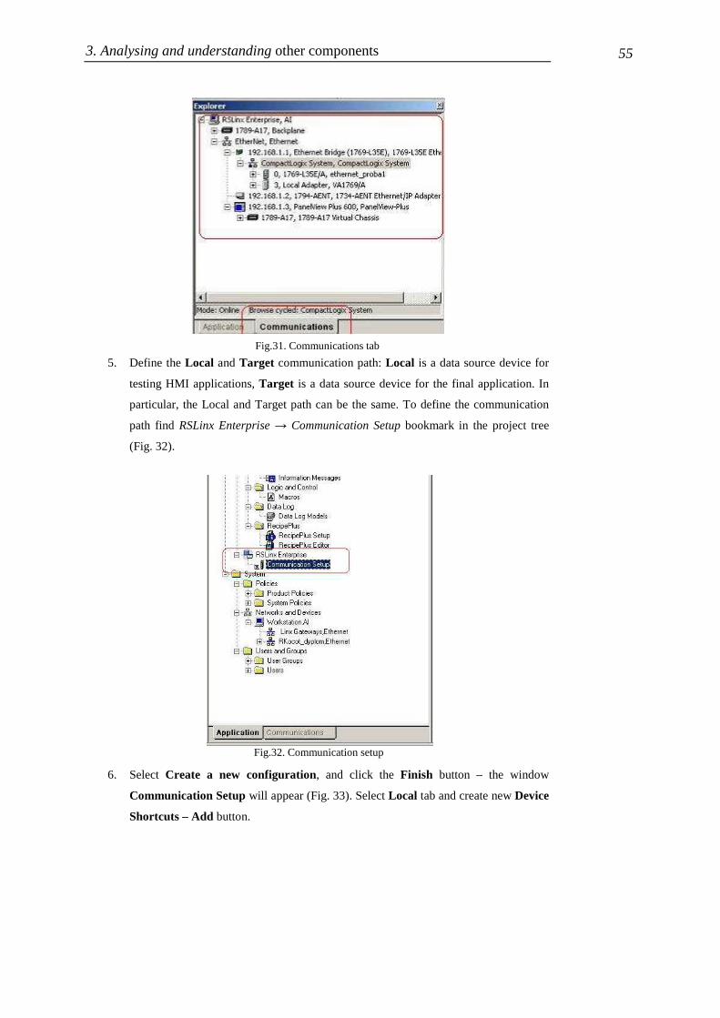
4. Prepare correct configuration of Communication. First check available devices. For

this purpose click the Communications tab (Fig. 31).

Fig. 30. Project Settings window

Fig. 29. Creating of the new PanelView project


54


5. Define the Local and Target communication path: Local is a data source device for

testing HMI applications, Target is a data source device for the final application. In

particular, the Local and Target path can be the same. To define the communication

path find RSLinx Enterprise → Communication Setup bookmark in the project tree

(Fig. 32).

6. Select Create a new configuration, and click the Finish button – the window

Communication Setup will appear (Fig. 33). Select Local tab and create new Device

Shortcuts – Add button.

Fig.32. Communication setup

Fig.31. Communications tab


56


As a local source device select the CompactLogix System. Target configuration we can copy from Local setting by using the Copy button.

7. To apply the configuration push the OK button.

Now we are ready for developing visualization of our process. First prepare a virtual display. ALARM, DIAGNOSTICS and INFORMATION displays are created automatically in the section Graphics->Displays. The new displays will be added there. To do this, right-click Displays – from the context menu and select New (Fig. 34).

A new empty window with edited display will be opened. We can add several graphic elements to visualize our process. You can find detailed descriptions of the available elements in [2] and [3]

Fig.34. Adding a new display

Fig.33. The Communicaton Setup window


58


As an example we can create a momentary pushbutton. For this purpose:

1. Select the Object → Push Button → Momentary item from the menu.

2. Left-click and drag the mouse pointer up to create a rectangle.

3. Double-click on the rectangle to open the Properties window. Set the appropriate

parameters such as: appearance, button settings, caption, etc.


60


4. Define the corresponding tag. Click the Connections tab and browse the data by

using Tag Browser. Refresh the actual folder – all available network tags will be

displayed.

Select the appropriate tag – now the pushbutton will be connected with the tag value.

Authors: D. Marchewka, M. Rosół

3.3 Bibliography

[1] Allen-Bradley. Adjustable Frequency AC Drive FRN 1.xx – 4.xx User Manual. Rock-well Automation, January 2007 [2] Rockwell Software. RS View Machine Edition. User's Guide vol.1, Rockwell Automa-tion, July 2005 [3] Rockwell Software. RS View Machine Edition. User's Guide vol.2, Rockwell Automa-tion, July 2005


62

4. Monitoring of the Ethernet/IP network traffic 63

4 Monitoring of the Ethernet/IP network traffic

Wireshark is a network packet analyser . It is used to: • troubleshoot network problems, • examine security problems, • debug protocol implementations, • learn network protocol internals.

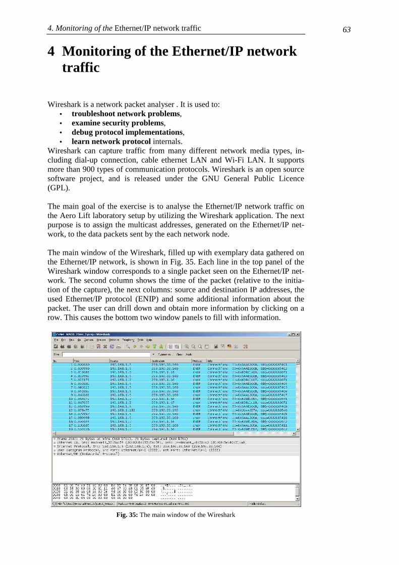
Wireshark can capture traffic from many different network media types, in-cluding dial-up connection, cable ethernet LAN and Wi-Fi LAN. It supports more than 900 types of communication protocols. Wireshark is an open source software project, and is released under the GNU General Public Licence (GPL). The main goal of the exercise is to analyse the Ethernet/IP network traffic on the Aero Lift laboratory setup by utilizing the Wireshark application. The next purpose is to assign the multicast addresses, generated on the Ethernet/IP net-work, to the data packets sent by the each network node. The main window of the Wireshark, filled up with exemplary data gathered on the Ethernet/IP network, is shown in Fig. 35. Each line in the top panel of the Wireshark window corresponds to a single packet seen on the Ethernet/IP net-work. The second column shows the time of the packet (relative to the initia-tion of the capture), the next columns: source and destination IP addresses, the used Ethernet/IP protocol (ENIP) and some additional information about the packet. The user can drill down and obtain more information by clicking on a row. This causes the bottom two window panels to fill with information.

Fig. 35: The main window of the Wireshark

4. Monitoring of the Ethernet/IP network traffic

64


For real-time messaging, Ethernet/IP employs the UDP over IP, which allows datagram to be multicast to a group of destination addresses. This producer-consumer multicast model is called “Implicit I/O Data connection” and pro-vides I/O data sending at regular time interval. Hence, to properly analyse the network traffic its necessary to understand the concept of multicast addressing, which is used in the Ethernet/IP protocol. IP multicast addresses (Layer 3 of the OSI) have been assigned to the old Class "D" address space by the Internet Assigned Number Authority (IANA). Addresses in this space are denoted with a binary "1110" prefix in the first four bits of the first octet, as shown in Fig. 36. This results in IP multicast addresses spanning a range from 224.0.0.0 through 239.255.255.255. The remaining 28 bits identify the multicast "Group" the datagram is sent to.

Octet 1 Octet 2 Octet 3 Octet 4 1110xxxx xxxxxxxx xxxxxxxx xxxxxxxx

Fig. 36: IP multicast address format All IP multicast frames, all MAC layer addresses beginning with the 24-bit prefix of 0x0100.5Exx.xxxx. With only half of these MAC addresses available for use by IP Multicast, 23 bits of MAC address space is available for mapping Layer 3 IP multicast addresses into Layer 2 MAC addresses. All Layer 3 IP multicast addresses have the first four of the 32 bits set to 0x1110, leaving 28 bits of meaningful IP multicast address information. These 28 bits must map into only 23 bits of the available MAC address. This mapping (for IP multicast equal to 239.192.1.65) is shown graphically in Fig. 37.

Fig. 37: Multicast MAC address mapping

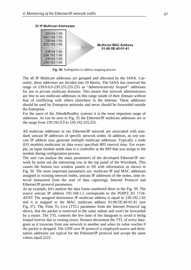
As can be shown in Fig. 37 the all 28 bits of a the Layer 3 multicast address cannot be mapped into the available 23 bits of MAC address space. This means that each IP multicast MAC address can represent 32 IP multicast addresses (32:1 address ambiguity when a Layer 3 IP multicast address is mapped to a Layer 2 MAC address). An example of the ambiguity in mapping process is shown in Fig. 38.


66


Fig. 38: Ambiguities in address mapping process

The all IP Multicast addresses are grouped and allocated by the IANA. Cur-rently, these addresses are divided into 10 blocks. The IANA has reserved the range of 239.0.0.0-239.255.255.255 as “Administratively Scoped” addresses for use in private multicast domains. This means that network administrators are free to use multicast addresses in this range inside of their domain without fear of conflicting with others elsewhere in the Internet. These addresses should be used by Enterprise networks and never should be forwarded outside the Enterprise. For the users of the Allen&Bradley systems it is the most important range of addresses. As can be seen in Fig. 35 the Ethernet/IP multicast addresses are in the range from 239.192.0.0 to 239.192.255.255. All multicast addresses in our Ethernet/IP network are associated with stan-dard, unicast IP addresses of specific network nodes. In addition, an one uni-cast IP address may generate multiple multicast addresses. Typically a node (I/O module) multicasts its data every specified RPI interval time. For exam-ple, an input module sends data to a controller at the RPI that you assign to the module during configuration process. The user can analyse the main parameters of the developed Ethernet/IP net-work by point out the interesting row in the top panel of the Wireshark. This causes the bottom two window panels to fill with information as shown in Fig. 39. The most important parameters are: multicast IP and MAC addresses assigned to existing network nodes, unicast IP addresses of the nodes, time in-terval (measured from the start of data capturing), Internet Protocol and Ethernet/IP protocol parameters. As an example, let's analyse the data frame numbered three in the Fig. 39. The source unicast IP address 192.168.1.2 corresponds to the POINT_IO 1734-AENT The assigned destination IP multicast address is equal to 239.192.1.65 and it is mapped to the MAC multicast address 01:00:5E:40:01:41 (see Fig. 37). The Time To Live (TTL) parameter from the Internet Protocol tag shows, that the packet is restricted to the same subnet and won't be forwarded by a router. The TTL controls the live time of the datagram to avoid it being looped forever due to routing errors. Routers decrement the TTL of every data-gram as it traverses from one network to another and when its value reaches 0 the packet is dropped. The UDP over IP protocol is employed source and desti-nation addresses are typical for the Ethernet/IP protocol and accept the same values equal 2222.


68


The Sequenced Address Item (0x8002), Connection ID (0x428e1a16), Con-nected Data Item (0x00b1) and item data length are the same for this type of transaction. The Data field length directly corresponds to the number of bytes transferred from the POINT_IO 1734-AENT.

Fig. 39: The Ethernet/IP network monitoring by utilizing the Wireshark


70


4.1 Exercise 1.

Assignment of multicast addresses to a specific transaction data exchange. The main goal of this exercise is to recognize of all multicast addresses as-signed to the Ethernet/IP network nodes and to analyse the tags of an Ethernet frames. All necessary data will be collected using the Wireshark program.

1. First, you have to be aware that all components are connected in a proper way (especially all Ethernet cables).

2. Run RSLinx Classic first and next RSLogix 5000. 3. Open an exemplary project. 4. Check if the local and network configuration has been correctly carried

out. The most important are the unicast IP addresses of each node and data exchanging between all network nodes.

5. In the next step set the PLC to the Run mode and download program to the program memory of the PLC. After downloading, if everything was setup correctly, the “I/O OK” indicator is green.

6. Run the Wireshark program and set capture interface in accordance with. Click the Start button next to the name of the interface on which you wish to capture traffic (or press the Capture -> Start option form the Main menu). The capture process will start immediately.

7. After a several seconds a running capture session should be stopped by pressing the Stop icon located on the toolbar or choosing the Capture -> Stop option form the Main menu.

8. Now, you can view all captured Ethernet frames, assigning a multicast addresses by reading source unicast IP addresses and analysing frame tags. It is important that one unicast IP address can generate a few mul-ticast addresses (each type of data transaction occupies a different mul-ticast address).


72


4.2 Exercise 2.

Analysis of the Requested Packed Interval (RPI) time. The main goal of this exercise is to experimentally analyse variation of the RPI, which decides about refreshing of I/O data over the Ethernet/IP network. All necessary data will be collected using the Wireshark program. The exercise assumes that students carried out the configuration of the Ethernet/IP network nodes and can check and change the value of the RPI.

1. Repeat steps 1-3 from the Exercise 1. 2. Read RPI parameter set for each I/O module (open the Module Prop-

erties window and select the Connection tag). For each RPI assign the unicast IP address of the corresponding module.

3. Repeat steps 5-7 from the Exercise 1. 4. Locate and write down all type of transactions with the same source and

destination addresses, for example: 192.168.1.5 – 239.192.33.160, 192.168.1.182 – 239.192.23.193 etc.

5. Order all of the frames according to the capturing time (the second col-umn of the main window of the Wireshark).

6. Read and write down times for the ten consecutive transactions of the same type.

7. Calculate the RPI by subtracting two consecutive capturing times wrote in step 6.

8. Compare the calculated values of the RPI with values set during the configuration stage.

9. Repeat steps 6-8 for all transactions of the same type.

conet mobile lab - agh university of science and...

Documents