computer simulation of diffusing-wave spectroscopy of colloidal dispersions and particle gels

Articles

Computer Simulation of Diffusing-Wave Spectroscopy ofColloidal Dispersions and Particle Gels

Christopher M. Wijmans,† David S. Horne,*,‡ Yacine Hemar,§ andEric Dickinson|

Department of Chemical Engineering, University of Amsterdam, Nieuwe Achtergracht 166,1018 WV Amsterdam, The Netherlands, Hannah Research Institute, Ayr KA6 5HL, U.K.,

Institute for Food, Nutrition and Health, Massey University, Palmerston North, New Zealand,and Procter Department of Food Science, University of Leeds, Leeds LS2 9JT, U.K.

Received June 15, 1999. In Final Form: March 24, 2000

A computational approach has been developed to model diffusing wave-spectroscopy (DWS) behaviorin colloidal systems. This model has been applied to the study of both colloidal dispersions and particlegels. The individual particle dynamics are computed from a Brownian dynamics simulation. Subsequently,a large number of photon paths through the system are generated. These paths, in combination with themean-square displacements of the particles obtained from the Brownian dynamics simulations, are usedto calculate the temporal autocorrelation function g(1)(t). The simulations reproduce the effect of the systemthickness on g(1)(t) for a stable colloidal dispersion as found experimentally, as well as the effect of thecomposition of a bimodal dispersion. Simulations of particle gels show how the gelation process influencesthe correlation function. These simulations reproduce the profound changes in the correlation functionseen experimentally during the gelation process and demonstrate that such effects are primarily due tochanges in the particle dynamics rather than in the large-scale topology of the developing network.

1. Introduction

Diffusing-wave spectroscopy (DWS) is a relatively newtechnique that is extremely useful for the study ofconcentrated colloidal systems, which cannot easily beinvestigated using traditional dynamic light scatteringtechniques because of the strongly multiple scatteringnature of such systems.1 An important application of DWSis the study of gelation processes. Because DWS meas-urements depend strongly on the dynamics of the scat-tering particles, DWS of gelling systems can providevaluable information on the extent and kinetics of thegelation process. Examples of this application of the DWStechnique are studies of the gelation of milk induced byenzyme treatment either alone2 or in combination withacidification,3 and measurements of latex particle mobilityin a gelatin solution as the solution is cooled through thesol-gel transition.4 In systems such as these, the gelationprocess slows the particle dynamics very considerably,and this profoundly affects the intensity autocorrelationfunction of the scattered light.

We have recently developed a computer simulation

model of particle gelation by Brownian dynamics.5 In thispaper we use this simulation model to predict DWScorrelation functions of gelling systems. Before using themodel, we test the DWS simulation algorithm by applyingthe model to the (simpler) case of particles undergoingunrestricted Brownian motion. An approach similar toours has been taken by Middleton and Fisher6 and byDurian7 to test approximate theories describing DWS. Themain difference between these papers and our presentsimulations is that we explicitly take account of anensemble of particles, which scatter the incident light,rather than assuming that photons are scattered atrandom points in space. The spatial positions of theparticles and their mobilities are derived from a separateBrownian dynamics simulation. Our main aim is todetermine the effect of gelation on the predicted dynamiclight scattering in a high volume fraction and thereforemultiple scattering situation. In addition, for comparisonpurposes, we first study the light scattering by a stabledispersion of colloidal particles.

Throughout this paper we restrict ourselves to thebackscattering geometry, which is commonly used in DWSexperiments. Experimentally, this geometry has theadvantage that it requires access to the sample only fromone side. However, the disadvantage of this geometrycompared with the transmission geometry lies in thetheoretical analysis of the temporal autocorrelation func-tion. Because many length scales are probed simulta-

* To whom correspondence should be addressed.† University of Amsterdam.‡ Hannah Research Institute.§ Massey University.| University of Leeds.(1) Weitz, D. A.; Pine, D. J. In Dynamic Light Scattering: The Method

and Some Applications; Brown, W., Ed.; OUP: Oxford, 1993; p 652.(2) Horne, D. S. In New Physico-Chemical Techniques for the

Characterization of Complex Food Systems; Dickinson, E., Ed.; Blackie:London, 1995; Chapter 11, p 240.

(3) Dalgleish, D. G.; Horne, D. S. Milchwissenschaft 1991, 46, 417.(4) Horne, D. S.; McKinnon, I. R. Prog. Colloid Polym. Sci. 1997, 104,

1163.

(5) Whittle, M.; Dickinson, E. Mol. Phys. 1997, 90, 739; Wijmans, C.M.; Dickinson, E. J. Chem. Soc., Faraday Trans. 1998, 94, 129; Wijmans,C. M.; Whittle, M.; Dickinson, E. In Food Emulsions and Foams:Interfaces, Interactions and Stability; Dickinson, E., Rodrı́guez Patino,J. M., Eds.; Royal Society of Chemistry: Cambridge, 1999; p 342.

(6) Middleton, A. A.; Fisher, D. S. Phys. Rev. B 1991, 43, 5934.(7) Durian, D. J. Phys. Rev. E 1995, 51, 3350.

5856 Langmuir 2000, 16, 5856-5863

10.1021/la9907681 CCC: $19.00 © 2000 American Chemical SocietyPublished on Web 06/10/2000

neously, it is less apparent that one can apply the diffusionapproximation to describe the light transport in thebackscattering geometry.1 By conducting simulations (aspresented in this paper), one can indeed test the theoreticalpredictions made using the diffusion approximation.

2. Simulation MethodIn a colloidal dispersion at relatively low concentrations

and short times, the mean-square particle displacement⟨∆r2(t)⟩ as a function of time t follows directly fromEinstein’s equation: ⟨∆r2(t)⟩ ) 6Dt, where D is the diffusionconstant. However, in a gelled system the particle motionis strongly restricted, so we need to conduct Browniandynamics (BD) simulations to study the particle kinetics.We consider here a system of N spherical particles in acubic simulation box of size l 3 with periodic boundaryconditions. From these simulations we can extract themean-square displacement of the particles ⟨∆r2(t)⟩ as afunction of time t. We then construct a slab of material,which we use for the simulated light-scattering experi-ments by considering a three-dimensional array of periodicimages of the system used in the BD simulation. In twodirections (x and y) the slab stretches out infinitely, andin the z-direction it has a finite thickness L, which is equalto an integer times the length l of the BD simulation box.(We denote the l 3-sized system used in the BD simulationas the “primary system” to distinguish it from the largersystem used in the DWS simulation.) We first describethe BD algorithm, and subsequently we discuss the DWSsimulation algorithm.

Brownian Dynamics Simulation. We consider Nspherical particles (typically, N is of the order 103-104)at a volume fraction φ. To model a stable colloidaldispersion, the interaction between two particles isrepresented as a steeply repulsive core potential φC, forwhich we use the following form:

In this equation εc is an energy parameter and rij ) |ri- rj| is the interparticle distance between the interactingparticles i and j. The particle diameter σ is used as thebasic unit of distance in the simulation model, and theenergy scale is defined by the parameter εc ) kBT. Thetime scale is defined by the relaxation time τr, which isthe time taken for a particle to diffuse a distance of halfthe particle diameter: τr ) (3πσ3ηs)/(4 kBT), where ηs isthe solvent viscosity. For a particle with diameter σ ) 1µm in water, the value of τr is 0.58 s.

The translational update algorithm is written as afunction of the interparticle forces:

where Fi is the force due to interparticle interactions, êis the Stokes friction coefficient, and Ri(t,∆t) is the familiarGaussian random displacement.

A space-filling, percolating network of particles (i.e., aparticle gel) is formed by the formation of bonds betweenthe particles. We define a probability PB that a bond isformed between two particles whose intersurface separa-tion is less than a critical distance b1. Such a bond resultsin an attractive force between bond nodes that are definedon the particle surfaces (at r ) σ/2) at points collinearwith the particle centers. This force is described by thefollowing bond potential φB:

where bij is the internode distance. As default values weuse εb ) 1.0, b1 ) 0.1, b0 ) 0.1, and bmax ) 1.0. Only onebond can be formed between any pair of particles. Theinitial alignment of the bond with the particle centerssoon disappears because of the subsequent motion of theparticles. The force due to the bond interaction must beadded to the interparticle force in eq 2. The bondinteraction also leads to a torque being exerted on theparticles. This is accounted for by a rotational updatealgorithm5 that is analogous to the translational updatealgorithm of eq 2. In addition to the bond interaction, wesometimes introduce an extra long-range interactionpotentialφLR, which has a strong influence on the structureof the gel that is formed. This potential has the form

and causes a constant force, which is attractive or repulsive(depending on the sign of εLR), between two particles ata separation smaller than the long-range cutoff distancerc (we use a default value of rc ) 2.5σ).

Whittle and Dickinson5 have demonstrated that themodel outlined above generates gel-like structures withfractal properties. The nature of these structures dependsstrongly on the parameters used, specifically on thebonding probability and the long-range interaction. Anattractive long-range interaction leads to a coarse gelstructure with a low fractal dimension, whereas a far finerstructure with a higher fractal dimension is formed for arepulsive interaction. For example, for PB ) 10-3 the fractaldimension is 1.85 for a long-range interaction parameterεLR ) -0.23 and 2.05 for εLR ) +0.23. The distribution ofpore sizes was also shown to be sensitive to the simulationparameters used. As the value of εLR increases, theoccurrence of large pores becomes more likely.

The parameter values used in this paper have beenchosen for consistency with earlier work. Especially, theparameters that determine the bond potential (eq 3) maybe expected to have a large influence on the mobility ofan individual particle in a gel. We will further addressthis issue in the Results section.

DWS Simulation Algorithm. A photon enters thesimulation box at z ) 0. The photon then moves in astraight line, and at regular sampling intervals we testwhether the photon has “hit” a particle (that is, comewithinadistanceof σ/2 fromaparticle center). If thephotondoes not hit any particle, it continues moving along astraight line, leaves the system at z ) L, and is discarded.If a photon hits a particle, then we have to decide itsscattering angle (θ) according to a probability distribution,P(x), defined by the Rayleigh-Gans-Debye formulationfor the particle-scattering form factor:

where x ) 2πσ/λ sin(θ/2) and λ is the wavelength of thelight. Unlike the formulation of Middleton and Fisher6

which considered point scatterers and isotropic scattering,our approach introduces scattering-angle probabilitiesdependent on the finite physical size of the particles. Suchprobability functions, when integrated over all scatteringangles, would yield the total scattering cross-section foran individual particle.

φC ) εC( σrij

)36(1)

ri(t + ∆t) - ri(t) ) Fi(t)∆tê

+ Ri(t,∆t) (2)

φB ) εb(bij - b1

b0)2

for bmax > bij > b1 (3)

φLR ) εLR

(rc - rij)

(rc - σ)for rij < rc (4)

P(x) ) 9x6

(sin x - x cos x)2 (5)

Computer Simulation of Diffusing-Wave Spectroscopy Langmuir, Vol. 16, No. 14, 2000 5857

After being scattered, the photon continues to move ina straight line in its new direction. At regular samplingintervals we test to determine whether the photon has hitanother particle, and if so, it is scattered again accordingto the distribution of eq 5. A photon that reaches the planez ) L is discarded (forward scattering). Only photons thatreturn to the plane z ) 0 (backscattering) are consideredin our calculations. Such photons may reach this plane bymany different paths, and the electric field at the detectoris taken as the sum of the fields due to each of these paths.The scattering particles, however, are in constant motion,and this causes the length of each path to vary over time.Because the phase of the scattering field that arrives atthe detector due to a particular path depends on the lengthof that path, this phase evolves in time and is themechanism giving rise to the time dependence of theautocorrelation function.

Following the formulation of Middleton and Fisher,6let us consider a single path R of a photon with a wavevector of magnitude k ) 2π/λ, collected at z ) 0 after havingundergone n scattering encounters with n particles. Wedefine kj

R - kj-1R as the transfer wave vector of the jth

encounter, with kjR as the wave vector after the jth event,

1 e j e n, |kjR| ) k. Again, following Middleton and Fisher,6

we note that the probability distribution for the changein path length during time t is Gaussian, with mean zeroand variance

where ⟨∆r2(t)⟩ is the mean-square displacement of theparticles. Because the scattering particles move slowlycompared to the speed of light, the absolute value of thewave vector k ) 2π/λ does not change when a photon isscattered. For paths involving only a few scatterers, thisGaussian form relies on the approximation that thescatterers execute independent random walks. For pathsinvolving many scatterers which undergo more correlatedbut isotropic random motion, Middleton and Fisher6 arguethat the same form will be obtained as a result of thesummation over many independent light paths, as longas the correlations are of finite range. Hence for our particlegels we use the value of the mean-square particledisplacement averaged over all particles that have thesame number of bonds.

The procedure described above is repeated until we havecollected Nba backscattered photon paths (and in themeantime discarded Nfo forward-scattered photon paths).We then calculate the temporal autocorrelation functiong(1)(t) from a summation over all backscattered paths:

In the simulation approach outlined above, the photonsenter the system under an angle of 90° over a limited area(a square with length of the order of 101 particle diameters),and they can exit the system at any point. This is thetime-reversed equivalent of an experiment with a planarlight source and a point detector. A point detector will inreality have a certain physical size, which is reflected bythe size of the primary simulation box. The fairly strictconstraints on the acceptance angle of the optical fiber tothe photomultiplier are reflected by the perpendicularangle of incidence in the simulation. Because the photonstravel at the speed of light, they have a negligible transit

time in the suspension. This fact justifies the principle oftime reversal.

Comparison with Theory. Pine and co-workers8 havederived an expression for the autocorrelation functionwithin the diffusion approximation (i.e., assuming thatthe light transport through the sample can be describedasa diffusion process). They used an initial condition givenby an instantaneous planar light source at a distance z) z0 from the illuminated surface. The boundary conditionswere specified by requiring that (for t > 0) the net flux ofdiffusing light into the sample be zero. This leads to thefollowing equation for the autocorrelation function g(1)(t):

where l * is the transport mean free path of the photons,and τ ) (k2D)-1 for diffusive motion. For infinite slabthicknesses and in the limit t , τ, eq 8 reduces to

3. Results and Discussion

We start by considering a system consisting of mono-disperse (unbonded) particles at a volume fraction φ )0.05. The mean-square displacement of the particlesfollows directly from the equation ⟨∆r2(t)⟩ ) 6Dt. We firstinvestigate such a system, rather than a more complicatedparticle gel, as a test for the DWS simulation method. Weuse a primary system with N ) 104 particles (l /σ ) 47.1).By conducting independent simulation runs with differentparticle configurations, we confirmed that the statisticalerror introducedbythe finite sizeof theprimarysimulationbox is negligible. Figure 1A shows simulated values forg(1)(t) which were computed for a wavelength equal to theparticle radius (λ ) σ/2). In this figure, the logarithm ofg(1)(t) has been plotted against xt for different systemsizes L: L ) 2l (curve “a”), 20l (curve “b”), and 2000l(curve “c”); in all cases, l /σ ) 47.1. For a particle diameterof ca. 1 µm, these values of the system size in reducedunits correspond to slab thicknesses of 0.1 mm, 1 mm,and 10 cm, respectively. In parts B and C of Figure 1,similar graphs are shown for a different particle concen-tration and wavelength. In Figure 1B the volume fractionis twice as high (φ ) 0.1; λ ) σ/2) and in Figure 1C thewavelength is twice as small (φ ) 0.05; λ ) σ/4).

The value of g(1)(t) is determined by the paths of thebackscattered photons only. For small values of the slabthickness L, this means that only short path lengths areaccounted for, where a photon is scattered by only arelatively small number of particles before it returns tothe plane of incidence at z ) 0. A large number of photonsare lost because they transit the slab and exit from theface parallel to the plane of incidence. As the slab thicknessincreases, the number of photon-particle encountersincreases. Longer path lengths, and also more of them,are taken into account and a larger proportion of theincident photons is backscattered. In the limit of infinite

(8) Pine, D. J.; Weitz, D. A.; Zhu, J. X.; Herbolzheimer, E. J. Phys.(Paris) 1990, 51, 2101.

(9) Horne, D. S. J. Phys. D 1989, 22, 1257.

yR ) ∑j)1

n

(kjR - kj-1

R)2⟨∆r2(t)⟩/6 (6)

g(1)(t) )⟨E(t)E*(0)⟩

E(0)2) ∑

R)1

Nba

exp(-yR) (7)

g(1)(t) ) {sinh[x6tτ ( L

l *-

z0

l *)] +

23x6t

τcosh[x6t

τ ( Ll *

-z0

l *)]}/{(1 + 8t

3τ) sinh[ Ll *x6t

τ ] + 43x6t

τcosh[ L

l *x6tτ ]} (8)

g(1)(t) ) exp[-z0

l *x6tτ ] (9)

5858 Langmuir, Vol. 16, No. 14, 2000 Wijmans et al.

slab thickness, all photons are backscattered and thedistribution of path lengths has an infinitely long tail. Wefind that for L ) 2l , actually only a minority of all incidentphotons are backscattered: for every 10 photons thatreturn to the plane z ) 0, 150 photons leave the systemat z ) L. However, for L ) 20l , on average only 8.4 photonsleave the system at z ) L for every 10 photons that returnto the plane z ) 0. For L ) 2000l the system virtuallyrepresents an infinitely thick slab, and in this case forevery 1000 backscattered photons there are, on average,fewer than 8 that are scattered in the forward direction.

Figure 2 shows the distribution of path lengths ofbackscattered photons for L ) 2l and for L ) 2000l. Thisdistribution isexpressed in terms of the fraction of collectedphotons that have suffered the plotted number of scat-tering events. In the case of the thin slab with L ) 2l , thisfractional distribution has a clear maximum at ap-proximately 25 scattering events, after which it falls offrelatively quickly. Less than 8% of all backscattered

photons have been scattered more than 50 times. Thelongest path length found in the simulation was 148scattering events. In contrast, for L ) 2000l the distribu-tion has a far more extended shape, with more than halfof all backscattered photons being scattered more than200 times. In this case, 8% of the photons are scatteredeven more than 10,000 times.

The influence of the contribution from the longer pathlengths (i.e., those with the higher number of scatteringevents), as a result of increasing slab thickness, can beinvoked to explain the changes in curvature in plots ofg(1)(t), as seen in Figure 1. The nonexponential characterof the correlation function betrays the existence of multipletime constants, indicative of differing decay rates in thepaths of various lengths. Paths involving large numbersof scattering events decay the most rapidly, because eachindividual particle in the chain needs to move only a shortdistance and takes a short time to do so. By contrast,paths made up of few scattering events decay more slowly,as the smaller number of particles must move relativelyfurther to reach an accumulated path-length change ofone wavelength. Thus, for small values of L, the data inFigure 1A show a strong curvature at low t, whichdisappears for larger values of L. This effect of the slabthickness is in good agreement with experimental find-ings.9 In Figure 1A another curve has been added, whichshows g(1)(t) as predicted by eq 9. A value of 1.72 has beenused for z0/l * to fit the slope of this line to that of thesimulated curve. In addition, log(g(1)(t)) has been shiftedupward slightly (by a value of 0.04) to get the best fitbetween both curves. The residual curvature in thesimulated curve shows up in the small difference betweenthis curve and the fitted line at small t.

The contribution of photon paths of different lengthtowards the correlation function is further explored inFigure 3. The curve in this figure that is labeled as “total”is the same as curve “a” in Figure 1A. This curve wasobtained by summing over all backscattered photon paths(eq 7). We have also drawn curves that show the resultwhen the summation is extended only over those pathsthat have 10 or fewer scattering events (“short”), and whenthe summation is over those paths that have more than50 scattering events (“long”). The decay length of the totalsignal is only slightly less than that of the short pathlengths only. However, the short path-length signal doesshow a very prominent concavity at short times.

In Figure 1B the particle concentration has beenincreased by a factor of 2 to φ ) 0.1. Qualitatively, thesame trends are found as for φ ) 0.05. However, g(1)(t)depends slightly less strongly on the slab thickness. AsL increases, g(1)(t) decreases less strongly than in the caseofφ) 0.05. Because of the increased particle concentration,

Figure 1. Correlation function g(1)(t) plotted against xt/τr fora stable colloidal dispersion. In (A) φ ) 0.05 and λ ) σ/2; in (B)φ ) 0.1 and λ ) σ/2; in (C) φ ) 0.05 and λ ) σ/4. The slabthickness has been varied: L ) 2l for curves “a”; L ) 20l forcurves “b”; and L ) 2000l for curves “c”. All simulations use aprimary system with 10 000 particles (so that l ) 47.1σ in (A)and (C) and l ) 37.4σ in (B)). In part (A) a curve is also shownwhich gives g(1)(t) according to eq 9 for z0/l * ) 1.9.

Figure 2. Path-length distributions of backscattered photonsfor the system of Figure 1A for L ) 2l (a) and L ) 2000l (b).


a photon is more likely to be backscattered in a systemwith the same slab thickness. The effect of the wavelengthon g(1)(t) can be seen in Figure 1C. In this figure φ ) 0.05,and the wavelength used is equal to half a particle radius(λ ) σ/4). A smaller wavelength (in relation to the particlesize) means that the average angle over which a photonis scattered is smaller (eq 5). As a consequence, one hasto go to larger slab thicknesses to reach the limitingbehavior for g(1)(t), and an increase in the slab thicknessleads to a larger decrease of g(1)(t) when the wavelengthis shorter. As light with a smaller wavelength is scatteredover a smaller angle, the backscattered photons have, onaverage, been scattered a larger number of times. Thiscauses the faster decay of g(1)(t) as compared to thecorrelation function in Figure 1A.

Up to now we have assumed that when a photon reacheseither of the planes z ) 0 or z ) L, it subsequently exitsthe system. However, if the photon is reflected, that willhave an effect on the photon path-length distribution. Wehave considered the case that there is a probability R thata photon is reflected at the z ) 0 boundary. In Figure 4the curve for R ) 0 is the same as curve “b” in Figure 1A(φ ) 0.05, L ) 20l ). The correlation function has also beensimulated for the same system with R ) 0.99. Increasingthe value of R shifts the photon path length distributiontoward longer path lengths. As a consequence g(1)(t)

decreases. At small t the curve of log(g(1)(t)) versus xtbecomes slightly convex rather than concave. At longertimes the curves are roughly parallel lines for differentvalues of R.

Bimodal Colloidal Dispersions. In general it isbelieved that, for a polydisperse system, diffusing-wavespectroscopy will give only an average relaxational mobil-ity for the particle size distribution. This is because thediffusing photon can encounter particles of any contribut-ingsizeonanycontributingpathway. InFigure5,however,we consider one more system consisting of unbondedparticles, where we explore the influence of “polydisper-sity” in a dispersion with two distinct particle populations,one with particle diameter 3 times the other (σ and 3σ,respectively). The total particle volume fraction, φ, whichis the sum of the volume fraction of the small particles,φ1, and that of the larger ones, φ2, is kept at a constantvalue of 0.1. For φ1 ) 0.1 and φ2 ) 0 we have the samesystem as studied in Figure 1B. For the opposite case thatall particles are large particles (φ1 ) 0 and φ2 ) 0.1) thefunction g(1)(t) decays more slowly and exactly reflects inits linear t1/2 behavior the lower diffusional mobility ofthose large particles. For these larger particles, however,the curvature in g(1)(t) at short decay times persists tomuch greater slab thicknesses. This result is consistentwith our observations, plotted in Figure 1C, where,although we halved the wavelength, the same effect wouldhave been seen by doubling particle size. In mixed systemsthe response of g(1)(t) to changes in the system compositionis very nonlinear. If a small fraction (5%) of the largerparticles is replaced by the same volume fraction of smallerones, this has a large effect on g(1)(t). However, replacinga far larger fraction (50%) of small particles by large oneshas only a very small effect. This same nonlinearity hasbeen observed experimentally for mixed systems ofpolystyrene latex particles with a similar particle sizeratio.9 The results can only be interpreted, however, inartificial systems such as these, where the input particlesize distribution is already known. DWS yields only asingle relaxation time. Attempting to extract more thanone piece of information is not physically feasible.

Comparison with Experiment. Finally, in Figure 6we compare experimental and simulated data for a latexdispersion. The circles are measurements of a 0.25-mm-thick sample of a 1.0 vol % dispersion of polystyrenespheres (330 nm diam) using a He-Ne laser (taken from

Figure 3. The effect of the photon path-length distribution ong(1)(t). The curve labeled as “total” is the same as curve “b” inFigure 1A, which is the correlation function for a system withφ ) 0.05 and λ ) σ/2. The “short” curve shows the correlationfunction as it is calculated when only photons that have beenscattered fewer than 11 times are taken into account. The “long”curve is calculated using only photons that have been scatteredmore than 50 times.

Figure 4. Correlation functions calculated for different re-flectivities of the z ) 0 boundary as defined by the parameterR (see text). Parameters: φ ) 0.05; λ ) σ/2; L ) 20l ; R ) 0 and0.99 (the curve for R ) 0 is the same as curve b in Figure 1A).

Figure 5. Correlation functions for a bimodal dispersion witha particle size ratio of 3. The wavelength is equal to the radiusof the smaller particles. In all cases the total particle volumefraction φ ) φ1 + φ2 ) 0.1. The volume fraction of the largerparticles φ2 is shown in the figure for each curve. Thecharacteristic time τr used to define the time axis is thecharacteristic diffusion time of the smaller particles.


ref 9). The squares are measurements on the same latexdispersion with a sample thickness of 2 mm. The simula-tion used a primary system with 2000 particles (l ) 47.1σ;L ) 16l, and L ) 128l ) and a wavelength of ) 1.44σ. Thedata in this figure show a good agreement betweenexperimental points and simulation (solid lines). Oneshould bear in mind that the experimental data havealways to be normalized, which leads to a (rather arbitrary)vertical shift of the data. Therefore, one should primarilycompare the slopes of the curves rather than their absolutevalues. The slopes do indeed show a good agreement.

Simulations of Particle Gel Behavior. We now turnour attention to a gelled system. We form a particle gelstarting with a random dispersion of unbonded particlesat a volume fraction φ ) 0.05. We use a bonding probabilityPB ) 10-3 for a time step ∆t/τr ) 10-6 to form a suitablenetwork of bonded particles.5 After a time ta (the gel age),the bonding probability is set to zero, stopping furtherbond formation and allowing us to study the dynamicalproperties of the particles in the network at that level ofbonding. In Figure 7 the average mean-square particledisplacement ⟨∆r2(t)⟩ is shown for two different values ofta. The line shows the mean-square displacement of a freelydiffusing particle. As particles become bonded, theirmobility decreases. For ta/τr ) 88, the value of ⟨∆r2(t )10τr)⟩ is only 4% of the value for a freely diffusing particle.Of course, the actual mobility of a particle in the gelnetwork depends on the parameters used in the bond

potential φB of eq 3. Here we used the (relatively arbitrary)values εb ) 1.0, b1 ) 0.1, and b0 ) 0.1. Using a strongerbond potential, for example εb ) 5.0 and b0 ) 0.01, givessmaller values for the mean-square displacement. Thiseffect of the bond strength is most important at relativelysmall times (≈10-2τr) and is relatively insignificant atlong times (≈10τr). At long times the displacement of anindividual particle is probably mainly determined by themovement of a cluster of surrounding particles. However,the choice of parameter values for the bond potential willcertainly have an effect on the initial decay of the DWSautocorrelation function. The values shown in Figure 7were found by averaging over all particles in the system.The average mean-square displacement of a particledecreases as the number of bonds between that particleand other particles increases. When simulating DWSexperiments, we therefore use a value for ⟨∆r2(t)⟩ for eachparticle that is found by averaging over all particles withthe same number of bonds.

The gelling system which gave rise to the data plottedin Figure 7 has also been used to compute the data for thecorrelation functions, g(1)(t), derived at the different gelages indicated and shown in Figure 8. The data for theunbonded particles (i.e., ta ) 0, curve “a”) are similar tothose in Figure 1A. After gelation, the correlation functiondecays more slowly because of the decreased particlemobility. The initial decay of g(1)(t) is relatively unaffectedby the gelation. At longer times the effect of the gelationbecomes more pronounced, and as the gel age increases,the relaxation time of the correlation function alsoincreases. We explained above that a different choice ofparameter values for the bond potential will lead todifferent values for g(1)(t). As the gel age increases, theshear modulus also increases. Previous simulations5

showed that the high-frequency shear modulus is a linearfunction of the number of interparticle bonds.

The statistical error in the data presented in Figure 8is mainly due to two sources. First, the finite length of theBrownian dynamics simulations leads to an uncertaintyin the values found for the mean-square particle displace-ments. For small times t this uncertainty is completely

Figure 6. Comparison between experimental data (circles,sample thickness 0.25 mm; squares, thickness 2 mm), takenfrom ref 9 and simulations (full curves) for a 1.0 vol %polystyrene latex with a particle diameter of 330 nm and awavelength (in the simulation) of λ ) 1.44σ.

Figure 7. Average mean-square displacements ⟨∆r2(t)⟩ ofparticles in a gel (φ ) 0.05) formed with PB ) 10-3 and εLR )0. The age of the gel is ta/τr ) 8.8 (9) and 88 (b). The line showsthe mean-square displacement of a freely diffusing particle.

Figure 8. Correlation functions for a gel formed with PB )10-3 and εLR ) 0. The curves “a”-“f” are for increasing gel ageta. Curve “a” is for ta ) 0, which corresponds to a dispersionconsisting of unbonded particles. Curve “b” ta/τr ) 2.2; curve“c”, ta/τr ) 8.8; curve “d” ta/τr ) 44; curve “e”, ta/τr ) 88; curve“f”: ta/τr ) 177. The data points for curves “b”-“f” are thesimulated values of g(1)(t) computed at values for the mean-square particle displacements identical to those employed inFigure 7. The curves themselves are interpolations betweenthese points. The simulations use a primary system with 1000particles and φ ) 0.05 (i.e., l ) 21.8σ). The slab thickness isL ) 50l ) 1.1 × 103 σ.


negligible, but it is more important for values of t thatbecome of a similar order of magnitude as the simulationlength. Second, the structure of a simulated gel is itselfsubject to fluctuations. As the gelation is necessarilysimulated using a finite system (103 particles), there willbe an uncertainty in the average number of bonds perparticle after gelation. Simulations using independentlygenerated particle configurations show that the statisticalerror in the curves of Figure 8 is negligible compared tothe differences between two different curves.

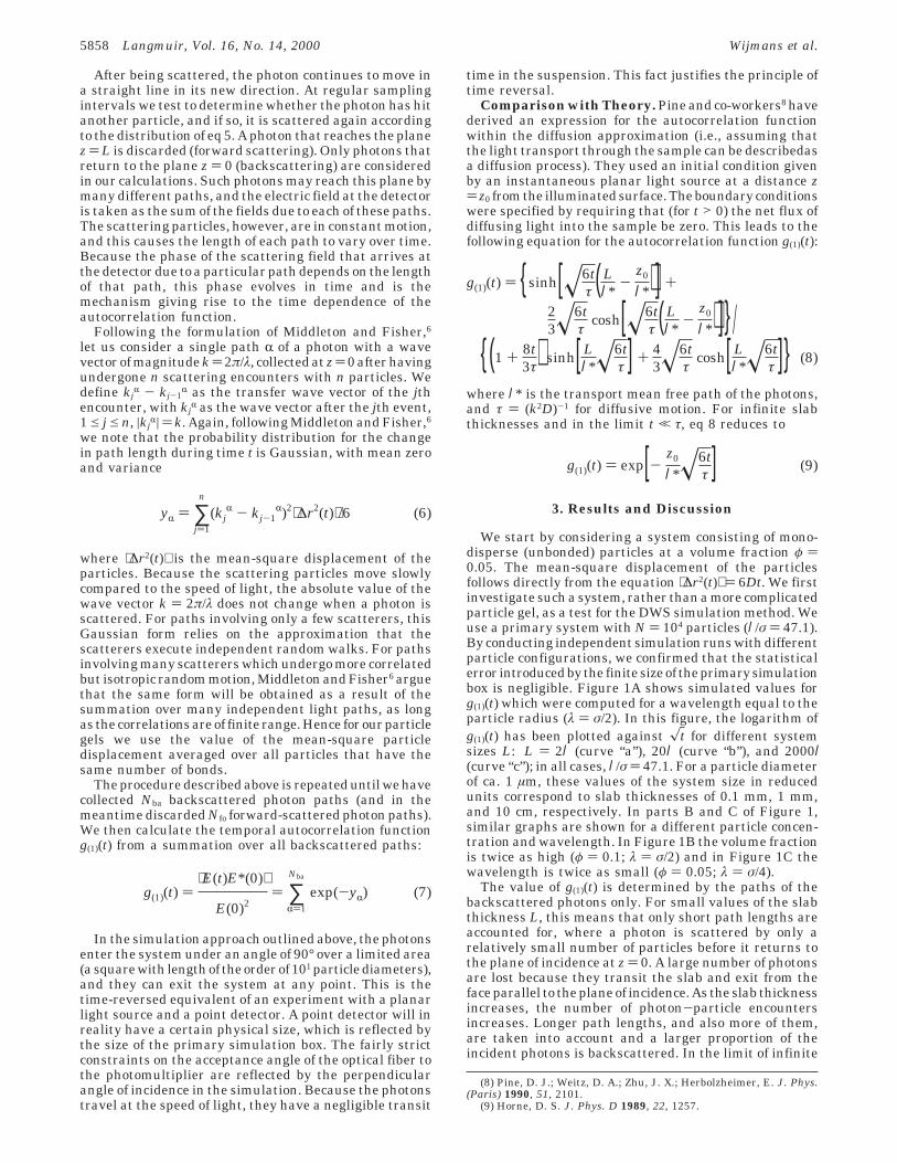
Figures 7 and 8 were calculated using a long-rangeinteraction parameter εLR equal to zero. If the gelationtakes place in a system with a different value for thisparameter, the resulting gel network will have a differentstructure. Simulations have shown5 that negative valuesof εLR give a coarser structure characterized by a lowerfractal dimension, and positive values give a less coarsestructure with a higher fractal dimension. In Figure 9simulated data are shown for gels with εLR ) -1 (coarse,low fractal dimension) and εLR ) 1 (fine-structured, higherfractal dimension). In the former case, the attractiveinterparticle forces promote the formation of bonds, thusdecreasing the average particle mobility in comparisonwith a gel for which εLR ) 0. The result is that the relaxationtime of the correlation function increases. In contrast,when εLR ) 1, fewer bonds are formed and the relaxationtime is shorter than for the case εLR ) 0.

Of course, differences in the correlation functions fordifferent values of εLR can be caused by differences in boththe gel structure and in the particle dynamics. Todetermine the relative importance of these two effects,we conducted the following simulation. We used the spatialpositions of the particles in the gels formed with εLR ) -1and εLR ) 1 for a simulated DWS experiment. However,in both cases we used exactly the same values for themean-square particle displacement. For this to be possiblethe gels must have different ages, and hence differentextents of bonding and network structures. In fact weselected the same value for ⟨∆r2(t)⟩ to all particles,regardless of the number of bonds on each particle. Anydifferences in g(1)(t) between the two gels must now becaused by the different structures of these two gels (asexpressed, for example, by differences in the radial paircorrelation function). In Figure 9 one can see that thevalues of g(1)(t) are virtually the same in both cases. Thisleads to the conclusion that the differences between thegels are caused by differences in the particle dynamicsand not by structural differences.

One note of caution should be made regarding the timescales of the gelation process and the decay of thecorrelation function. Not too much importance should beattached to the absolute values found in the simulations.In our Brownian dynamics simulations, the gelationkinetics are primarily determined by the parameter PB,which gives the probability for two particles to form abond when they are at a small separation. In addition, theinteraction potential will have an important influence onthe gelation. We have chosen to use a simple pair potentialwhich only accounts for the repulsion between twoparticles when they start to overlap. In principle, it isfeasible to include an activation energy that must beovercome when two particles approach each other,10 whichslows the gelation. In this way it would certainly bepossible to get a better fit between the simulated gelationand the kinetics of a real system, but this was not theprimary aim of our investigation. The main result of thesimulations is the strong increase in the correlationfunction relaxation time as the gelation progresses; thisincrease is not affected by the precise details of the gelationkinetics.

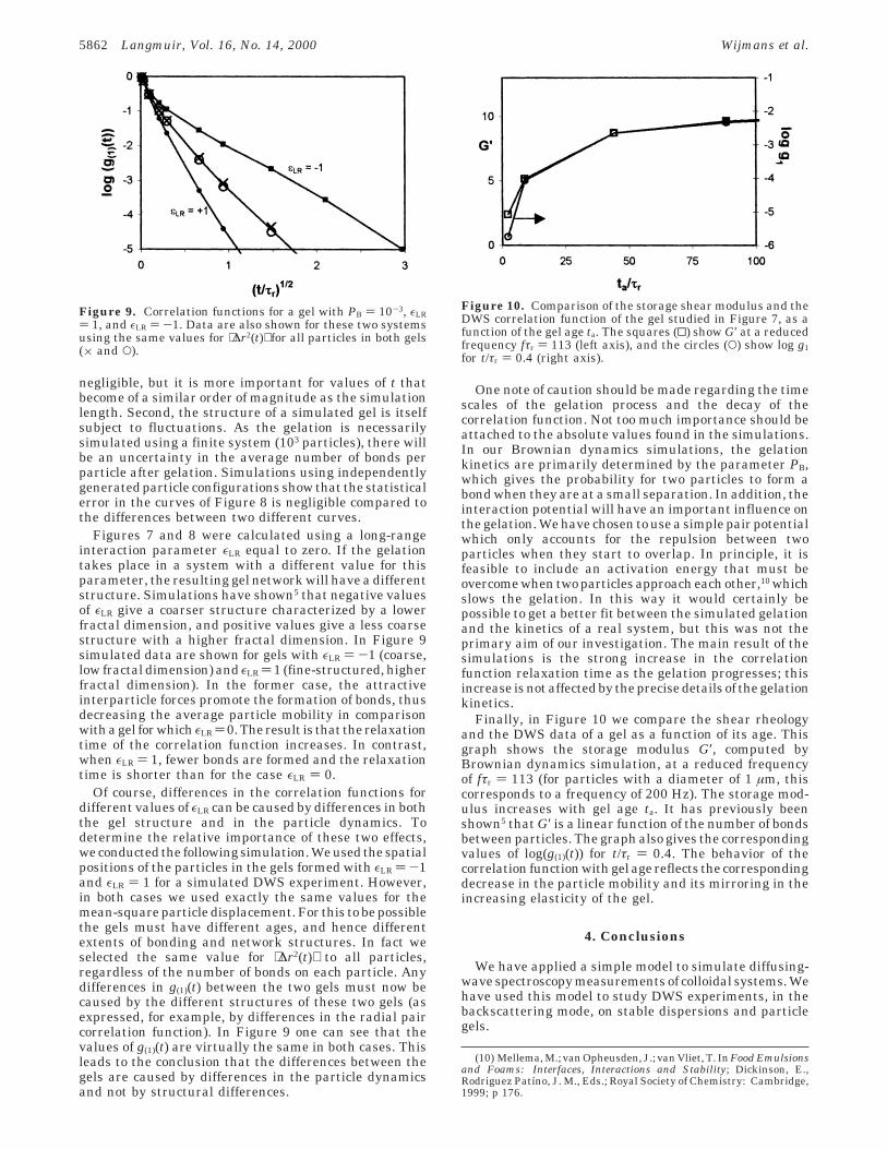
Finally, in Figure 10 we compare the shear rheologyand the DWS data of a gel as a function of its age. Thisgraph shows the storage modulus G′, computed byBrownian dynamics simulation, at a reduced frequencyof fτr ) 113 (for particles with a diameter of 1 µm, thiscorresponds to a frequency of 200 Hz). The storage mod-ulus increases with gel age ta. It has previously beenshown5 that G′ is a linear function of the number of bondsbetween particles. The graph also gives the correspondingvalues of log(g(1)(t)) for t/τr ) 0.4. The behavior of thecorrelation function with gel age reflects the correspondingdecrease in the particle mobility and its mirroring in theincreasing elasticity of the gel.

4. Conclusions

We have applied a simple model to simulate diffusing-wave spectroscopy measurements of colloidal systems. Wehave used this model to study DWS experiments, in thebackscattering mode, on stable dispersions and particlegels.

(10) Mellema, M.; van Opheusden, J.; van Vliet, T. In Food Emulsionsand Foams: Interfaces, Interactions and Stability; Dickinson, E.,Rodriguez Patı́no, J. M., Eds.; Royal Society of Chemistry: Cambridge,1999; p 176.

Figure 9. Correlation functions for a gel with PB ) 10-3, εLR) 1, and εLR ) -1. Data are also shown for these two systemsusing the same values for ⟨∆r2(t)⟩ for all particles in both gels(× and O).

Figure 10. Comparison of the storage shear modulus and theDWS correlation function of the gel studied in Figure 7, as afunction of the gel age ta. The squares (0) show G′ at a reducedfrequency fτr ) 113 (left axis), and the circles (O) show log g1for t/τr ) 0.4 (right axis).


The simulations of dispersions reproduce the charac-teristic effect of the slab thickness on the correlationfunction g(1)(t) that is found experimentally. Furthermore,the simulations show the same nonlinearity of g(1)(t) asafunction of system composition that has been foundexperimentally for bimodal dispersions.

The simulations of particle gels show how the decay ofg(1)(t) slows dramatically during the gelation process. Thisis a direct consequence of the self-diffusion of the gellingparticles, which become increasingly more restricted in

their movement as the gelation progresses. Differencesbetween gels with different structures have been shownto be due primarily to differences in the individual particledynamics rather than to structural differences.

Acknowledgment. This work was supported byContract FAIR-CT96-1216 of the European Union Frame-work IV Programme.

LA9907681


computer simulation of diffusing-wave spectroscopy of colloidal dispersions and particle gels

Documents