computational simulation of fracture repair in stem cell

University of Calgary

PRISM: University of Calgary's Digital Repository

Graduate Studies The Vault: Electronic Theses and Dissertations

2012-09-28

Computational Simulation of Fracture Repair in Stem

Cell Seeded Defects under Different Mechanical

Loading

Nasr, Saghar

Nasr, S. (2012). Computational Simulation of Fracture Repair in Stem Cell Seeded Defects under

Different Mechanical Loading (Unpublished master's thesis). University of Calgary, Calgary, AB.

doi:10.11575/PRISM/25397

http://hdl.handle.net/11023/242

master thesis

University of Calgary graduate students retain copyright ownership and moral rights for their

thesis. You may use this material in any way that is permitted by the Copyright Act or through

licensing that has been assigned to the document. For uses that are not allowable under

copyright legislation or licensing, you are required to seek permission.

Downloaded from PRISM: https://prism.ucalgary.ca

UNIVERSITY OF CALGARY

Computational Simulation of Fracture Repair in Stem Cell Seeded Defects under Different

Mechanical Loading

by

Saghar Nasr

A THESIS

SUBMITTED TO THE FACULTY OF GRADUATE STUDIES

IN PARTIAL FULFILMENT OF THE REQUIREMENTS FOR THE

DEGREE OF MASTER OF SCIENCE

DEPARTMENT OF MECHANICAL AND MANUFACTURING ENGINEERING

CALGARY, ALBERTA

September 2012

© Saghar Nasr 2012

i

Abstract

Mechanical factors play a key role in regulation of tissue regeneration during skeletal healing,

but the underlying mechanisms are not fully understood. The objective of the current study was

to explore the role of mechanical factors on tissue differentiation during fracture healing, using a

biphasic mechanoregulatory algorithm. The first specific objective was to investigate the effect

of mechanical loading on a stem cell seeded collagenous scaffold in a one-dimensional confined

compression configuration. Both empirical and computational data suggest that mechanical

stimulation of the scaffold may be an effective way to initiate differentiation pathways prior to

implantation for tissue engineering applications. The second objective was to predict the

development of differentiated tissues in a tibia burr-hole fracture murine model with

computational mechanoregulatory algorithms. The computational and experimental studies will

be used simultaneously in future studies to further develop mechanoregulatory models with a

more robust quantitative base.

ii

Acknowledgements

Blessed Be His Name

First I must thank Dr. Neil A. Duncan for his tremendous dedication and guidance throughout

the duration of this investigation. Without his support, this work would not have been possible.

I want to thank my amazing parents, sister, brother, grandparents, and my uncle, Shahriar, for

their love and unwavering support. My thanks are also extended to Drs. Leonard Hills and

Mojtaba Kazemi for their encouragements and valuable comments.

This research was supported by a team grant from the Canadian Institutes of Health Research in

Skeletal Regenerative Medicine, the Natural Sciences and Engineering Research Council and the

Canada Research Chair in Orthopaedic Bioengineering.

iii

Table of Contents

Abstract ........................................................................................................................... i Acknowledgements ......................................................................................................... ii

Table of Contents ........................................................................................................... iii List of Tables ................................................................................................................. vi

List of Figures and Illustrations .................................................................................... viii List of Symbols, Abbreviations and Nomenclature ....................................................... xix

CHAPTER ONE: INTRODUCTION .............................................................................. 1 1.1 Background and motivation ................................................................................... 1

1.2 Bone ...................................................................................................................... 4 1.2.1 Bone repair .................................................................................................... 9

1.2.1.1 Biological stages of fracture healing ................................................... 10 1.2.1.2 Source of progenitor cells for fracture healing .................................... 13

1.3 Problem statement and rationale .......................................................................... 14 1.4 Thesis objectives ................................................................................................. 22

1.5 Thesis overview .................................................................................................. 26

CHAPTER TWO: MECHANOREGULATION ALGORITHMS OF TISSUE

DIFFERENTIATION IN BONE .......................................................................... 28 2.1 Pauwels theory .................................................................................................... 29

2.2 Interfragmentary strain theory ............................................................................. 31 2.3 Mechanostat theory, (Frost, 1987) ....................................................................... 32

2.4 Computational simulations of tissue differentiation ............................................. 34 2.4.1 Single solid phase model (Carter‟s theory, 1988) ......................................... 34

2.4.2 Single solid phase model (Claes and Heigele, 1999) .................................... 37 2.4.3 Single solid phase model (Gardner et al., 2000) ........................................... 38

2.4.4 Biphasic model (Kuiper et al., 1996-2000) .................................................. 39 2.4.5 Biphasic model (Prendergast et al., 1997). ................................................... 41

2.4.6 Biphasic model (Sandino and Lacroix, 2011)............................................... 43 2.4.7 Models with biological factors ..................................................................... 45

CHAPTER THREE: DEVELOPMENT AND VERIFICATION OF THE FINITE

ELEMENT MODEL ............................................................................................ 61

3.1 Bone mechanics .................................................................................................. 61 3.1.1.1 Osteoporotic bone mechanics ............................................................. 65

3.1.2 Bone structure and optimisation .................................................................. 69 3.1.3 Mechanical behaviour of cortical bone ........................................................ 72

3.1.4 Mechanical behaviour of cancellous bone .................................................... 75 3.2 Soft tissue biphasic theory ................................................................................... 76

3.2.1 Kinematics .................................................................................................. 78 3.2.2 Conservation of mass .................................................................................. 80

3.2.3 Conservation of linear momentum ............................................................... 81 3.3 Finite element model of mechanoregulation ........................................................ 85

iv

3.3.1 Adaptive mechanoregulation algorithm ....................................................... 85 3.3.1.1 User defined subroutine: USDFLD..................................................... 88

3.3.1.2 Smoothing process ............................................................................. 91 3.3.1.3 Diffusion of progenitor cells............................................................... 92

3.4 Verification of the implemented model ................................................................ 99 3.4.1 Results ...................................................................................................... 102

3.4.2 Discussion ................................................................................................. 107 3.5 Fracture healing case studies ............................................................................. 108

3.5.1 An axisymmetric idealized murine model .................................................. 109 3.5.1.1 Results ............................................................................................. 111

3.5.1.2 Discussion ........................................................................................ 113 3.5.2 A 3D idealised model of murine tibia ........................................................ 114

3.5.2.1 Results ............................................................................................. 115 3.5.2.2 Discussion ........................................................................................ 117

3.6 Summary of the computational analyses ............................................................ 119

CHAPTER FOUR: COLLAGENOUS SCAFFOLD UNDER CONFINED COMPRESSION

........................................................................................................................... 122 4.1 Confined compression loading device description.............................................. 122

4.2 Computational modelling of the system ............................................................. 126 4.2.1 The cell base and the top lid ...................................................................... 127

4.2.2 The collagen gel and the porous plug ......................................................... 127 4.2.3 The silicone rings ...................................................................................... 129

4.3 Validation of the computational model against the experimental results ............. 131 4.3.1 The square-cross-section ring .................................................................... 131

4.3.2 The circular-cross-section ring................................................................... 132 4.3.3 The system excluding the collagenous gel ................................................. 134

4.3.4 The system including the collagenous gel .................................................. 136 4.4 Mechanical behaviour of the collagen gel in confined compression: cyclic loading143

4.5 Prediction of tissue differentiation in confined compression .............................. 149 4.6 Summary ........................................................................................................... 154

CHAPTER FIVE: TISSUE DIFFERENTIATION IN A BURR-HOLE FRACTURE

MODEL IN A MURINE TIBIA ......................................................................... 156

5.1 Introduction ....................................................................................................... 157 5.2 Reconstruction of a murine tibia ........................................................................ 158

5.2.1 Importing and preparing the data (ScanIP module) .................................... 158 5.2.2 Image processing (ScanIP module) ............................................................ 158

5.2.3 Creating the volumetric model, assigning material properties and mesh generation

(ScanFE module) ....................................................................................... 163

5.2.4 Convergence study .................................................................................... 167 5.3 Verification of the generated FE model of the intact tibia .................................. 168

5.4 Development of the burr-hole fracture model .................................................... 170 5.4.1 Selection of the decay length model........................................................... 173

5.5 Tissue differentiation predictions within the burr-hole fracture .......................... 178

v

5.5.1 Investigation of axial compression load ..................................................... 182 5.5.2 Influence of cell diffusivity rate ................................................................. 187

5.5.3 Influence of fracture position ..................................................................... 190 5.5.3.1 Different mechanical stimuli with the same cell origins .................... 190

5.5.3.2 Different mechanical stimuli and cell origins .................................... 193 5.5.4 Influence of reduced mechanical properties ............................................... 195

5.5.5 Influence of bending load .......................................................................... 199 5.6 Summary and discussion ................................................................................... 201

CHAPTER SIX: CONCLUSIONS, LIMITATIONS AND FUTURE DIRECTIONS .. 209 6.1 Summary and conclusions ................................................................................. 209

6.2 Limitations ........................................................................................................ 213 6.3 Future directions ................................................................................................ 217

REFERENCES ........................................................................................................... 219

APPENDIX A: USER DEFINED SUBROUTINE: USDFLD ..................................... 231

vi

List of Tables

Table 2.1. Mechanoregulatory stimulus for tissue differentiation (Prendergast et al. 1997). ....... 42

Table 2.2. Biphasic model prediction of tissue differentiation by Sandino and Lacroix (2011)... 44

Table 2.3. Summary of the mechanoregulatory algorithms of musculoskeletal tissue

differentiation. ................................................................................................................... 59

Table 3.1. The quantitative commutative tomography outcomes at the distal woman tibia

(Macdonald et al. 2011). .................................................................................................... 69

Table 3.2. Estimation of normal stress under axial, bending and torsional loads. ....................... 71

Table 3.3. Poroelastic tissue material properties (Isaksson et al. 2006)....................................... 88

Table 3.4. Dependence of material properties on field variable (FV) in the fracture site............. 90

Table 3.5. Applying the smoothing process to the algorithm. ..................................................... 92

Table 3.6. Similarity between mass diffusion and heat transfer equations. ................................. 95

Table 3.7. Element type, poroelastic and thermal properties of the tissues of a human. .............. 96

Table 3.8. Dimensions of the axisymmetric FE model of an ovine tibia. .................................. 101

Table 3.9. Geometry of the murine tibia proximal section (Windahl et al. 1999, Geris et al.

2004). .............................................................................................................................. 110

Table 3.10. Material properties used for the study (Rho, Ashman and Turner 1993, Isaksson

et al. 2006). ..................................................................................................................... 111

Table 4.1. Poroelastic properties of the porous plug and the collagen gel (Isaksson et al.

2006, Tromas et al. 2012). ............................................................................................... 129

Table 4.2. The geometry of the silicone rings. ......................................................................... 130

Table 4.3. The predicted equilibrium strains, fluid velocities and pore pressure at the peak

loading in the top, middle and bottom sample elements. .................................................. 149

Table 4.4. Poroelastic tissue material properties (Isaksson et al. 2006)..................................... 150

Table 5.1. The relationship between the mechanical properties and mass density (Rho et al.

1995). .............................................................................................................................. 165

Table 5.2. The range of greyscale based material properties of the murine tibia. ...................... 166

vii

Table 5.3. Convergence study for three mesh densities. ........................................................... 168

Table 5.4. Elements numbers for different parts of the fracture model. .................................... 171

Table 5.5. Summary of the variables for the parametric studies. .............................................. 180

Table 5.6. Element numbers and material properties used for the current study (Rho et al.

1993, Isaksson et al. 2006). .............................................................................................. 181

Table 5.7. Mechanical properties used for an osteoporotic murine tibia (Li and Aspden

1997b, Lacroix 2000, Macdonald et al. 2011, Sun et al. 2008, Isaksson et al. 2006). The

values can be contrasted to those for healthy bone in Table 5.6. ....................................... 197

viii

List of Figures and Illustrations

Figure 1.1. Cortical and trabecular bone shown in a µCT cross-sectional view of a murine

tibia. ....................................................................................................................................5

Figure 1.2. µCT images of vertebrae from two patients: (a) Normal bone in a 74 year old

woman (b) osteoporotic bone in a 94 year old woman (Cole et al. 2010). ........................... 10

Figure 1.3. Fracture healing stages: (a) inflammation, (b) callus differentiation, (c)

ossification, (d) remodelling (Bailon-Plaza and van der Meulen 2001)............................... 13

Figure 1.4 The essential tissues involved in fracture healing (Einhorn 2005). ............................ 14

Figure 1.5. (a) Sheep tibia subjected to torsion. (b) Histological section showing the

cartilaginous formation in the interfragmentary gap and the bony tissue in the internal

and external callus (Bishop et al. 2006).............................................................................. 17

Figure 1.6. (a) Lateral loading of the left knee, (b) µCT images of burr-holes in control

group with delayed healing, and (c) loaded group with promoted healing. Bar = 1 mm

(Zhang and Yokota 2011). ................................................................................................. 19

Figure 1.7. µCT images demonstrating the healing process and bone regeneration during 4

weeks: (a) in the control group, (b) collagenous scaffold seeded with ES cell-derived

osteoblasts implanted into the fracture site (Taiani 2012). Bar = 1 mm. ............................. 19

Figure 1.8. Both experimental and computational studies are required to fully understand the

tissue behaviour under mechanical loads and develop mechanoregulatory algorithms

(Epari, Duda and Thompson 2010). ................................................................................... 22

Figure 1.9. Objectives of the current study based on the in vitro collagenous scaffold and in

vivo burr-hole murine model. ............................................................................................ 23

Figure 1.10. Location of the burr-hole in the medial aspect of the tibia: (a) reconstructed FE

model based on the in vivo study, (b) µCT image of the in vivo model (Taiani 2012). A

section through the long axis of the burr-hole looking proximally: (c) reconstructed FE

model based on the in vivo study and (d) µCT image (Taiani 2012). .................................. 25

Figure 2.1. Types of the mechanoregulatory algorithms. ........................................................... 29

Figure 2.2. A schematic of Pauwels' theory, octahedral shear stress and hydrostatic pressure

used as biophysical stimuli (Pauwels 1960). ...................................................................... 30

Figure 2.3. Strain tolerance of different types of tissues (Tubbs 1981). ...................................... 31

Figure 2.4. Graph shows the mechanostat theory proposed by Frost (Frost, 2003). The

relationship between the tissue strain level and change in bone mass is presented. AW,

MOW and POW refer to the dead zone, mild overload and excessive load, respectively.

ix

MESm and MESp are the bone modelling and the micro-damage thresholds,

respectively. Fx is the bone fracture strength. These setpoints vary between individuals

and are hypothesised to be genetically determined. ............................................................ 33

Figure 2.5. The effect of mechanical loading and vascularity on bone differentiation (Carter

et al. 1988). ....................................................................................................................... 36

Figure 2.6. Carter s me hano iology theory. rin ipal tensile strain and hydrostati stress

history are the key iophysi al stimuli (Carter and eaupr 2001). .................................... 37

Figure 2.7. Single phase model introduced by Claes et al. (1999) in which hydrostatic

pressure and strain are the key biophysical stimuli. ............................................................ 38

Figure 2.8. Biphasic model introduced by Kuiper et al. (2000a), using fluid shear strain and

stress as the biophysical stimuli. ........................................................................................ 40

Figure 2.9. Proposed biphasic algorithm by Lacroix et al. (2002) in which octahedral shear

strain and fluid velocity are the biophysical stimuli. ........................................................... 42

Figure 2.10. Biphasic model introduced by Sandino and Lacroix (2011) in which fluid shear

stress and octahedral shear strain were used as biophysical stimuli. ................................... 44

Figure 2.11. (a) The relationship between the sprout branching and the sprout length, (b) the

rate of sprout growth as a function of mechanical stimulus (Checa and Prendergast

2009). ................................................................................................................................ 51

Figure 2.12. Mechanoregulatory algorithm proposed by Checa and Prendergast (2009)

simulating tissue differentiation by both the local mechanical environment and the

presence of oxygen from nearby blood vessels................................................................... 51

Figure 2.13. The mechanobiological algorithm proposed by Isaksson et al. (2008) simulating

tissue differentiation according to local mechanical environment, cellular events and

matrix production. ............................................................................................................. 53

Figure 2.14. Mechanoregulatory algorithm proposed by Sandino and Lacroix (2011)

simulating tissue differentiation based on mechanical stimuli, cellular events and

angiogenesis. ..................................................................................................................... 55

Figure 2.15. Schematic of the algorithm used by Nagel and Kelly (2010) to incorporate

collagen fibre orientations.................................................................................................. 57

Figure 3.1. Summary of model development and verification. ................................................... 61

Figure 3.2. The force-displacement plot representing bone behaviour (Cole et al. 2010). ........... 62

x

Figure 3.3. Relationship between the mineral content and bone mechanical properties: (a) by

increasing the mineral density, the stiffness increases, (b) while an increase in the bone

mineral content leads to more brittleness (Currey 2012)..................................................... 64

Figure 3.4. Variation of bone mass in men and women across the lifespan (McDonnell et al.

2007). ................................................................................................................................ 65

Figure 3.5. The material properties of a femoral osteoporotic (OP) bone were compared to

normal bone: (a) bone stiffness, (b) the yield strength, (3) bone density, and (d) the

absorbed energy of the bone decreases in osteoporotic bone (Li and Aspden 1997a). ......... 66

Figure 3.6. The radiographs of the proximal humerus in (a) a 87-year-old man with low bone

mineral density and, (b) a 65-year-old man with higher mineral density (Tingart et al.

2003). ................................................................................................................................ 67

Figure 3.7. The graph demonstrates the relationship between porosity and age for men and

women (McCalden et al. 1993). ......................................................................................... 68

Figure 3.8. The relationship between stiffness and density of the subchondral bone plate (Li

and Aspden 1997b). ........................................................................................................... 68

Figure 3.9. Excessive torque may cause a spiral fracture (a), tension causes transverse

fracture (b), oblique fracture may be created by compression (c), and butterfly fragments

may result from bending (d) (Giotakis and Narayan 2007). ................................................ 70

Figure 3.10. Variation in the size and mass distribution affects the bending stiffness of bone.

The middle figure represents a young bone with thicker cortical shell, whereas the bone

with thinner cortical shaft, at the right, represents an adult bone. In the older bone,

resorption of the inner surface and apposition of the outer surface decreased the bone

thickness. The bone mass was distributed further from the bending plane compared to

the young bone. ................................................................................................................. 72

Figure 3.11. The stress-strain curve illustrates that bone is stiffer in the longitudinal direction.

Young‟s modulus is the same in tension and ompression, whereas in ompression one

has more strength (Kutz 2003). .......................................................................................... 73

Figure 3.12. Young‟s modulus and ultimate stress of tibial cortical bone decrease with

increasing age. The rate of decrease is higher for ultimate stress compared to the

modulus (Burstein et al. 1976). .......................................................................................... 74

Figure 3.13. The response of cortical bone under different strain rates (Kutz 2003). .................. 75

Figure 3.14. The stress-strain plot for a load-unload-reload trabecular sample. The loading

starts at point 1, it is unloaded at point 2 and reloaded at point 3. The initial Young‟s

modulus from the linear section of the reloading (3-4) is the same as the original

xi

Young‟s modulus (1-2) at the beginning, but reduces quickly to residualE . A permanent

residual strain residualε will be developed (Keaveny, Wachtel and Kopperdahl 1999). .......... 76

Figure 3.15. (a) Movement of fluid when tissue is under a free draining confined

compression test, (b) ramp deformation is applied (increased with a linear ramp to B and

remained constant from B to E, (b) the flow exudes immediately after the deformation is

applied and the stress reaches its maximum amount (B). The fluid continues to flow.

The tissue reaches an equilibrium point and the stress decreases and reaches a plateau

(E) (Mow et al. 1980). ....................................................................................................... 78

Figure 3.16. Proposed biphasic algorithm by Prendergast et al. (1997); strain and fluid

velocity are the biophysical stimuli. ................................................................................... 87

Figure 3.17. The iterative model used to simulate fracture repair. .............................................. 88

Figure 3.18. A partial input file showing how the field variable was defined in the input file. .... 91

Figure 3.19. The profiles of (a) temperature and (b) fluid velocity are shown under the same

boundary condition show the same pattern (Cussler 2009). ................................................ 95

Figure 3.20. (a) Axisymmetric model of a human tibia, the radius of the cortical and bone

marrow are 15 and 9 mm (at the left). The cortical, bone marrow and callus are shown in

red, grey and green, respectively, (b) three origins for progenitor cells are shown.

Arrows indicate the cell origins (at the right). .................................................................... 96

Figure 3.21. (a) Cell concentration within the callus at two time points: 0.5s and 1 s, (b) cell

concentration over time in three sample elements, (c) the cell concentration at two time

points through the callus. ................................................................................................... 97

Figure 3.22. Schematic of the implemented algorithm to predict tissue distribution. The

coupled diffusive-poroelastic analysis for the mechanical stimulus and cell

concentration were obtained for each element (ABAQUS). ............................................... 99

Figure 3.23. The axisymmetric model of an ovine tibia with 3mm fracture gap and an

external callus: (a) Isaksson et al. (2006), and (b) the present study: bone marrow (in

red), cortical bone (in orange) and callus (in blue) are modelled. ..................................... 101

Figure 3.24. Prediction of fracture healing in the present study during 50 steps (days).

Cortical bone was subjected to a 300 [N] axial compression load (1 Hz). ......................... 104

Figure 3.25. The change of fluid flow [ m/s] over time under the cortical shaft and callus tip

during fracture healing. Cortical bone was subjected to a 300 N axial compression

loading (1 Hz). ................................................................................................................ 105

Figure 3.26. Comparison of the two simulations during fracture healing in the first steps.

Cortical bone was subjected to a 300 N axial compression loading (1 Hz): (a) the present

xii

study, and (b) Isaksson et al. (2006). In both models, intramembranous ossification

occurred at the callus tip and periosteum. Also, fibrous tissue and cartilaginous tissue

can be found in the same zones. ....................................................................................... 105

Figure 3.27. Comparison of the two simulations during fracture healing at step 50, cortical

bone was under 300 N axial compression loading (1 Hz): (a) the present study, (b)

Isaksson et al. (2006). The amount of fibrous tissue decreased significantly under the

cortical shaft. The distribution of mature and intermediate bone distribution is almost

identical. .......................................................................................................................... 106

Figure 3.28. Overall similar healing patterns were observed over time under a 300 [N] axial

compression load in (a) the present study, and (b) Isaksson et al. (2006). ......................... 107

Figure 3.29. (a) Axisymmetric FE model of a murine tibia (bone marrow in red, cortical bone

in grey and callus in blue), (b) the amplitude of the applied cyclic axial compression

loads. ............................................................................................................................... 109

Figure 3.30. Predicted tissue differentiation in the present study under (a) 0.5 N, (b) 1 N and

(c) 2 N axial compression load (1 Hz). ............................................................................. 112

Figure 3.31. Predicted mechanical stimuli for a sample element under the cortical shaft

during the healing process for three axial compression loading magnitudes. .................... 113

Figure 3.32. a) Axisymmetric FE model of a murine tibia. The inner and outer diameter of

cortical bone (gray) and external callus (blue) are 1, 1.5 and 2.4 mm, respectively, b)

Predicted tissue differentiation in the present study, c) CT images from Gardner et al.

(2006) for different load magnitudes (1 Hz). .................................................................... 114

Figure 3.33. The sample elements considered within three regions of the callus (external and

internal callus, and the interfragmentary gap). ................................................................. 116

Figure 3.34.Prediction of mechanical stimuli at three sample points, when bone is subjected

to axial torsion. The sample element under the cortical shaft has the highest mechanical

stimuli. ............................................................................................................................ 116

Figure 3.35. (a) A 3D FEM of a murine tibia with 0.4 mm gap, predicted tissue

differentiation in the model under: (b) Axial torsion (8 degree, 1 Hz), (c) Axial torsion

& compression (8 degrees, 0.45 MPa, 1 Hz). ................................................................... 117

Figure 3.36. (a) Sheep tibial section subjected to torsion (histological slide) (Bishop et al.

2006), (b) predicted tissue differentiation subjected to torsion (day 15, in the present

study). ............................................................................................................................. 118

Figure 3.37. Summary of the computational simulations in the current study. .......................... 121

Figure 4.1. FX-4000 ™ Flex ell ® ompression plus ™ system. ............................................. 123

xiii

Figure 4.2. Schematic of the Flexcell system cross-section in the uncompressed and

compressed configurations............................................................................................... 124

Figure 4.3. Parts of the modified system: (1) cell base, (2) square ring, (3) porous plug, (4)

round ring, (5) lid, and (6) fixed lid.................................................................................. 125

Figure 4.4. The modified system to conduct confined compression test. .................................. 126

Figure 4.5. The parts added to the modified Flexcell system. ................................................... 127

Figure 4.6. The force-displacement curve of the rings obtained from a uniaxial compression

test (Olesja Hazenbiller, M.Sc. Student, University of Calgary). ...................................... 131

Figure 4.7. The axial displacement [mm] of the axisymmetric model of the square ring under

30 N axial compression load at t=30 s. The inner and outer diameters are 10.7 mm and

12.7 mm, respectively, and the height is 1 mm. ................................................................ 132

Figure 4.8. The axial displacement [mm] of the axisymmetric model of the round ring under

30 N axial compression load at t=30 s. The inner and outer diameters are 6 mm and 10

mm, respectively, and the radius of the cross section is 2 mm. ......................................... 133

Figure 4.9. The axial displacement [mm] of the axisymmetric FE model of the system

without gel under 30 N axial compression load at t=30 s. The diameter of the porous

plug is 12.7 mm and the height is 3.175 mm. ................................................................... 135

Figure 4.10. Comparison of load-displacement curves between the FE and experimental

results under axial compression load applied at a rate of 1 N/s. ........................................ 136

Figure 4.11. The axisymmetric FE model of the modified Flexcell system. ............................. 137

Figure 4.12. (a) The contact surface at the beginning of the analysis, (b) if no adjustment

zone was used, ( ) the adjustment „a‟ was defined and the nodes within the zone were

moved onto the master surface (ABAQUS v6.11 user manual). ....................................... 138

Figure 4.13. Model predictions of the force-displacement curve for the whole system

including the collagen gel under confined compression: ramp load with the rate of 1 N/s. 140

Figure 4.14. Distribution of axial strain (EE2) and fluid velocity (FLVEL, [mm/s]), within

the collagenous scaffold under 20 N axial compression load at t=20 s.............................. 141

Figure 4.15. Change of fluid velocity over time within four sample elements of the

collagenous scaffold. The scaffold was loaded at a rate of 1 N/s. Four sample elements

are shown through the depth of the collagen (at the right). ............................................... 142

Figure 4.16. Change of axial strain over time within four sample elements of the collagenous

scaffold The scaffold was loaded at a rate of 1 N/s. Four sample elements are shown

through the depth of the collagen (at the right). ................................................................ 142

xiv

Figure 4.17. The load-displacement behaviour of the gel can be observed by comparing: (1)

the whole model including the gel, and (2) the whole model without the gel. The

deformation of the square ring decreased, while the deformation of the round ring was

independent from the gel and did not change. .................................................................. 143

Figure 4.18. The amplitude of the applied cyclic axial compression loads. The pressure,

ranging from 5-20 [kPa], was applied to the cell base with a frequency of 1 Hz. .............. 144

Figure 4.19. Model prediction for the axial strain during confined compression: cyclic

loading (P=5 kPa, 1 Hz). Compressive strain in top element under axial compression. ..... 145

Figure 4.20. Prediction of axial strain at the peak loading in three selected sample elements in

the collagenous scaffold in confined compression under cyclic loading of P=5 kPa (1

Hz). ................................................................................................................................. 145

Figure 4.21. Prediction of octahedral shear strain at the peak loading in three selected sample

elements in the collagenous scaffold in confined compression under cyclic loading of

P=5 kPa (1 Hz). ............................................................................................................... 146

Figure 4.22. Prediction of fluid velocity at the peak loading in the top sample element in the

collagenous scaffold in confined compression under cyclic loading of P=5 kPa (1 Hz). ... 146

Figure 4.23. Prediction of pore pressure at the peak loading in three selected sample elements

in the collagenous scaffold in confined compression under cyclic loading of P=5 kPa (1

Hz). ................................................................................................................................. 147

Figure 4.24. Comparison of axial strains at the peak loading in the top sample element in the

collagenous scaffold in confined compression under different cyclic applied loads of

P=5, 10, 20 kPa (1 Hz). ................................................................................................... 148

Figure 4.25. The gel was subjected to 10 kPa pressure (1 Hz). The hysteresis of the stress-

strain curve shows the effects of the interstitial flow and viscous dissipation (the graph

shows the first 33 seconds of analysis). ............................................................................ 148

Figure 4.26. Schematic of tissue differentiation algorithm. ...................................................... 151

Figure 4.27. Prediction of fluid velocity at the peak loading in three sample elements in the

collagenous scaffold during tissue differentiation (P = 20 kPa, 1 Hz). .............................. 152

Figure 4.28. Mechanical stimuli in a sample element at the superficial layer for a 5 kPa and a

20 kPa (1 Hz) compressive pressure applied to the system. .............................................. 153

Figure 4.29. (a) Gel before and after loading, (b) FE prediction of tissue differentiation (a 20

kPa compressive stress, 1 Hz). ......................................................................................... 154

Figure 4.30. Compressive load significantly influenced chondrogenesis (Col 2-day 15),

(Olesja Hazenbiller, M.Sc. student, University of Calgary). ............................................. 154

xv

Figure 5.1. Overview of this chapter. ....................................................................................... 157

Figure 5.2. Top view of sample holder is located fitted within the diameter of the field of

view (orange lines), (b) schematic of the sample holder used for scanning the murine

tibia (µCT 35, User Manual). ........................................................................................... 159

Figure 5.3. Cortical and trabecular bone could be visually distinguished in the µCT cross-

sectional view of a murine tibia. ...................................................................................... 161

Figure 5.4. Bone geometry before and after applying the recursive Gaussian filter. ................. 162

Figure 5.5. Cross-sectional view showing the cortical bone, bone marrow and trabecular

bone. ............................................................................................................................... 163

Figure 5.6. Illustrated are the masks for five different locations: (a) proximal tibia (b)

proximal tibial diaphysis, (c) tibial crest diaphysis, (d) midshaft, (e) distal tibia; Red,

blue and yellow masks represent cortical, trabecular and bone marrow, respectively........ 163

Figure 5.7. Lateral, medial, posterior, and anterior views of the finite element model of the

reconstructed murine tibia................................................................................................ 166

Figure 5.8. (a) Volume image, (b) greyscale data, (c) segmented mask, (d) isolated

segmented mask, (e) smoothed mask (recursive Gaussian filter), (f) mesh generation of

the extracted volume. ....................................................................................................... 167

Figure 5.9. Three zones that were compared: zone 1 (proximal tibia), zone 2 (tibial crest),

zone 3 (distal tibia). ......................................................................................................... 169

Figure 5.10. Force-strain relations measured by (a) Stadelmann et al. (2009), and (b)

predicted in the present study. .......................................................................................... 169

Figure 5.11. The distribution of principal strains when the tibia was subjected to a 10 N axial

compression load. ............................................................................................................ 170

Figure 5.12. Location of the burr-hole in the medial aspect of the tibia: (a) FE model, (b)

experimental fracture model (Taiani 2012). A section through the long axis of the burr-

hole: (c) FE model, (d) experimental fracture model (Taiani 2012). A section through

the frontal plane of the fractured tibia: (e) FE model, (f) experimental fracture model

(Taiani 2012). .................................................................................................................. 172

Figure 5.13. Workflow diagram outlining the required functions to reconstruct the 3D FE

burr-hole model. .............................................................................................................. 173

Figure 5.14. Overview of the processes used to create the burr-hole model. ............................. 173

xvi

Figure 5.15. The decay length models were subjected to a 10 N load to select the one that had

the closest mechanical environment compared to the full-length model. The red arrow

shows where the load was applied. .................................................................................. 174

Figure 5.16. Distribution of von Mises stress: (a) full-length model, (b) decay length model

(tibial crest, medial view). ............................................................................................... 175

Figure 5.17. Distribution of principal strains: (a) full-length model, (b) decay length model

(tibial crest, medial view). ............................................................................................... 176


(tibial crest, lateral view). ................................................................................................ 177

Figure 5.19 Distribution of von Mises stress within the scaffold: (a) full-length model, (b)

decay length model (tibial crest, medial view). ................................................................ 177

Figure 5.20 Distribution of principal strains within the scaffold: (a) full-length model, (b)

decay length model (tibial crest, medial view). ................................................................ 178

Figure 5.21. (a) Origins of the progenitor cells, (b) sample elements in the middle section and

top surface. ...................................................................................................................... 183

Figure 5.22. Mechanical stimuli of an outer radial sample element at the mid-section of the

scaffold (at peak load). Tibia was subjected to axial compression loads of 2, 1, and 0.5

N (1 Hz). ......................................................................................................................... 183

Figure 5.23. Mechanical stimuli of two sample elements at outer radial side of the scaffold

(at peak load): (1) mid-section, and (2) proximal surface. The tibia was subjected to a 2

N (1 Hz) axial compression load. ..................................................................................... 184

Figure 5.24. Mechanical stimuli of three sample elements located on the proximal surface of

the scaffold (at peak load): (1) outer radial, (2) middle, and (3) inner radial zone. The

tibia was subjected to a 2 N (1 Hz) axial compression load. ............................................. 184

Figure 5.25. The predicted interfragmentary strain, at peak load, under the cortical shaft for

the three loading cases (2, 1, 0.5 N axial compression, 1 Hz). .......................................... 185

Figure 5.26. Predicted fracture healing patterns under the 2, 1 and 0.5 N (1 Hz) axial


Figure 5.27. Cross-sectional view of the scaffold showing the accelerated healing of the core

compared to the outer layers. The tibia was subjected to a 2 N (1 Hz) axial compression

load. ................................................................................................................................ 187

xvii

Figure 5.28. The prediction of octahedral shear strain for different cell diffusion rates (0.025

and 0.01 s

mm2

). .............................................................................................................. 189

Figure 5.29. Predicted fracture healing patterns under the 1 N (1 Hz) axial compression load

for different rates of cell diffusion (0.025 and 0.01 s

mm2

)............................................... 189

Figure 5.30. Axial positions of the burr-hole fracture: (a) 2.55 mm and (b) 3.13 mm from the

proximal end. Both fractures are located in the trabecular bone and the tibia was

subjected to a 1 N (1 Hz) axial compression load. Bar = 0.7 mm. .................................... 191

Figure 5.31. Predicted mechanical stimuli in the outer radial location on the proximal surface

of the scaffold for two different hole positions: 3.13 mm versus 2.55 mm from the

proximal end. The tibia was subjected to a 1 N (1 Hz) axial compression force................ 192

Figure 5.32. Predicted fracture healing patterns for the two positions of burr-hole fractures.

The tibia was subjected to a 1 N (1 Hz) compression load................................................ 192

Figure 5.33. Cross sections of the 3.13 mm and 2.55 mm fracture cases at day 13. The 3.13

mm fracture case had slightly accelerated healing. Both tibiae were subjected to a 1 N

axial compression load (1 Hz).......................................................................................... 192

Figure 5.34. The origins of progenitor cells when the fracture is located in the bone marrow. .. 193

Figure 5.35. Predicted mechanical stimuli for two locations of the fracture (outer radial

sample element on the proximal surface): (1) in trabecular bone and (2) in bone marrow.

Tibia was subjected to a 2.5 N (1 Hz) compression load. ................................................. 194

Figure 5.36. The predicted tissue pattern for two locations of the fracture with different cell

origins: in trabecular bone, and in bone marrow. The proximal end of tibia was

subjected to a 2.5 N (1 Hz) compression load. ................................................................. 195



values can be contrasted to those for healthy bone in Table 5.6. ....................................... 197

Figure 5.37. The predicted mechanical stimuli at peak load for the osteoporotic and normal

bone. Tibia was subjected to a 2.5 N (1 Hz) axial compression load. ............................... 198

Figure 5.38. The predicted interfragmentary strain under the cortical shaft, at peak load, for

the osteoporotic and normal bone. Tibia was subjected to a 2.5 N (1 Hz) axial


Figure 5.39. The predicted tissue patterns for fracture repair within osteoporotic versus

normal bone. Tibia was subjected to a 2.5 N (1Hz) axial compression load. ..................... 199

xviii

Figure 5.40. Red arrow shows the bending load that was applied to the tibia. The distal end

was fixed and the hole size was 0.7 mm. Bar = 0.7 mm. .................................................. 200

Figure 5.41. Predicted mechanical stimuli for the outer radial sample element at located at the

proximal surface of the scaffold. The tibia was subjected to 0.04 and 0.02 Nm (1 Hz)

bending loads. ................................................................................................................. 201

Figure 5.42. Predicted tissue pattern for the murine tibia subjected to bending loads of 0.04

and 0.02 Nm (1 Hz). ........................................................................................................ 201

Figure 5.43. The gradual change of tissue type during the healing period within a young

(D=0.025 s

mm 2

), and an old murine tibia (D=0.01 s

mm 2

). ............................................ 204

Figure 5.44. The overall stiffness of the scaffold during the healing process for young and old

murine tibia with different diffusion rates (D=0.025 s

mm 2

and D=0.01

s

mm 2

). ............. 204

Figure 5.45. Histological slides (Day 7): (a) a large and (b) a small amount of cartilage were

present in the fracture site of young and elder murine tibia, respectively. In the

histological slides, cartilage is shown in red (Lu et al. 2005). In the computational study

(Day 7) similarly, more cartilaginous tissue differentiated in the younger murine tibia (c,

d). .................................................................................................................................... 205

Figure 5.46. The gradual change of tissue type during the healing period within a normal and

an osteoporotic murine tibia. ............................................................................................ 206

Figure 5.47. The overall stiffness of the scaffold during the healing process for normal and

osteoporotic bone. ........................................................................................................... 207

Figure 5.48. The healing progression in a normal bone and an osteoporotic bone from CT

images show that the normal bone had more mineralisation (Taiani 2012). ...................... 207

Figure 5.49. CT images showing the healing process within the burr-hole fracture model of

the (a) unloaded murine tibia, (b) tibia under bending load of 0.02 Nm (Zhang et al.

2007). .............................................................................................................................. 208

xix

List of Symbols, Abbreviations and Nomenclature

Roman letters

B Body force per unit mass

Cp Specific heat coefficient

D Diffusion rate,

E

Hydrostatic stress

Young‟s modulus

e Void ratio

GS Greyscale value

I Osteogenic index

J Deformation gradient

K Diffusive drag coefficient

k Fluid permeability,

Thermal conductivity

kc

n

Contact permeability

Porosity

p Fluid pore pressure

Ra Source of mass

S Octahedral shear stress,

Biphasic mechanical stimulus,

T

Specific matrix surface

Temperature

t Time

V

v

Volume

Fluid velocity

W Strain energy

Matrices and vectors

I Identity matrix

k Permeability tensor

q Fluid flow

T Deviatoric shear tensor

u Displacement

v Velocity

w Relative fluid displacement

Strain

Local body force

Stress

xx

Greek letters

Thermal diffusivity

Octahedral shear strain,

Specific weight

Stretch ratio

, Lamè material constants

Micro

oisson‟s ratio

Density

τ Fluid shear stress

Superscripts

f Fluid

s Solid

1

Chapter One: Introduction

1.1 Background and motivation

Bone is a complex, composite tissue composed of a mineralized component, and soft

extracellular matrix proteins, with dynamic interactions between these components across

multiple scales (Carter et al. 1998). This dynamic tissue has an exceptional ability to self-heal

throughout life. In healthy bone, there is a consistent balance between bone resorption and bone

formation. However, bone diseases or aging may affect the factors regulating this process, and

result in an altered bone micro-architecture, bone loss and reduced structural strength, making

bone more prone to fracture (McDonnell, McHugh and O'Mahoney 2007, Currey 2012, Jepsen

and Andarawis-Puri 2012).

The treatment and prevention of bone fracture is a global health problem for difficult-to-heal

fractures that can occur in osteoporotic elderly individuals. It is generally accepted that the rate

of fractures increases substantially with age (Knopp et al. 2005, Egermann, Goldhahn and

Schneider 2005). It has been estimated that at least 40 % of women and 15 % of men suffer from

a bone fracture after age 65 (Riggs, Khosla and Melton 2002). According to Gullberg et al.

(1997) hip fractures are set to increase by 310 % and 240 % for men and women by 2050,

respectively.

To better preserve the quality of life of afflicted individuals, research has focused on

understanding the mechanisms involved in the maintenance and repair of the musculoskeletal

system in order to improve treatment of broken bones. It is well known that bone is able to

optimise its mechanical properties to different physical conditions, including during fracture

repair, yet the mechanisms initiating and regulating bone maintenance and repair are not clearly

known (McMahon, O'Brien and Prendergast 2008, Morgan et al. 2010). Non-ideal mechanical

2

conditions and cell-matrix interactions may disrupt the process of healing and lead to non-unions

and cell apoptosis (Kwong and Harris 2008, Geris et al. 2009, Einhorn 2005). Therefore,

effective positive mechanical factors are encompassed by the range and frequency of the applied

loads.

The effect of frequency on bone regeneration, ranging from 1 to 20 Hz, has been investigated

computationally at the bone-implant interface (Geris et al. 2009). A bone chamber was used to

allow for controlled implant axial displacement of up to 90 µm. Bone tissue formation was

predicted using a biphasic mechanoregulatory algorithms (Lacroix et al. 2002, Prendergast,

Huiskes and Soballe 1997) and was compared with histology (Vandamme et al. 2007, Duyck et

al. 2006). In contrast to findings in orthopaedic implant osseointegration (Rubin and McLeod

1994), lower frequencies (in the order of 1 Hz) were predicted to promote bone formation.

According to Geris et al. (2009), frequencies above 1 Hz did not promote bone formation, the

bone chamber was mostly filled with soft tissue, and less bone-to-implant contact was observed.

Rubin and McLeod (1994) compared loading frequencies of 1 and 20 Hz to investigate the effect

of loading rate on bone growth and reported that the 20 Hz loading case promoted bone growth

into the implant pores whereas the 1 Hz loading case delayed the differentiation process.

Goodship et al. (1998) showed that a higher rate of loading promoted healing in the primary

stages, but delayed the process in the later healing stages. This may be due to the viscoelastic

nature of the tissue. During the initial stages, the higher rates of movement increased the fluid

velocity and promoted fibrous tissue differentiation. However, the high loading rates inhibited

bone formation later in the healing process (Goodship et al. 1998). Further experimental and

computational studies are essential to verify the real effect of frequencies and loading rates on

bone stimulation and growth.

3

New bone regeneration is also related to the magnitude and direction of the loads, however, the

mechanisms of transduction of the mechanical stimuli into a biological response remains unclear

(Isaksson et al. 2008, van der Meulen and Huiskes 2002). High magnitudes of load were shown

to result in delayed healing caused by the persistence of cartilage not differentiating into bony

tissue (Claes and Heigele 1999, Einhorn 2005). Isaksson et al. (2006) showed that increasing the

load delayed healing and a further increase led to: (1) a non-union, (2) having fibrous tissue in

the interfragmentary gap and (3) cartilaginous tissue in the external callus. A comprehensive

understanding of the mechanobiology of tissue formation, could improve treatment techniques to

better prevent non-unions and accelerate the healing process.

The bioengineering of tissue-engineered constructs offers a promising treatment of fractures

where stem cells and scaffolds are combined to enhance bone repair. Central to the success of

these initiatives is a detailed understanding of how stem cells respond to and interact with

mechanical cues from the bone and the biomaterial scaffold as they differentiate into mature

tissue. A number of empirically-based mechanobiology algorithms have been proposed to predict

tissue differentiation that incorporates mechanical factors. Experiments to evaluate the effect of

mechanical regimes on tissue regeneration are expensive and time consuming. To more

comprehensively understand tissue regeneration, computational models have been developed to

determine the mechanical and physical conditions within healing tissues. Empirically-based

algorithms have been implemented into computational models to predict bone tissue formation.

A number of different algorithms have been proposed and are based on different mechanical

factors, e.g., fluid hydrostatic pressure, interstitial fluid flow, and tissue strain (Prendergast et al.

1997, Sandino and Lacroix 2011, Isaksson et al. 2008). These algorithms are correlated with

experimental in vivo studies to determine which factors involved to simulate the healing process.

4

Improved validation of these algorithms can enhance our understanding of tissue

mechanobiology and lead to development of more sophisticated algorithms. The computational

predictions can then be used to design better clinical treatment options for bone fracture

treatment. These algorithms have been used to understand the mechanobiology of a number of

clinical applications including (1) prediction of tissue differentiation during fracture healing in

long bones (Lacroix et al. 2002, Isaksson et al. 2008), (2) modelling the bony in-growth on the

surface of bone implants (Geris et al. 2004, Moreo, Garcia-Aznar and Doblare 2009a, Moreo,

Garcia-Aznar and Doblare 2009b), (3) prediction of the tissue regeneration pattern in a multi-

scale model of a lumbar vertebral fracture (Boccaccio, Kelly and Pappalettere 2011), (4)

understanding the process of bone healing in trabecular bone (Shefelbine et al. 2005), and (5)

improving the design of scaffolds for bone tissue engineering (Kelly and Prendergast 2005,

Milan, Planell and Lacroix 2010, Byrne et al. 2007).

The underlying mechanisms that are responsible for a promoted bone healing are still unknown.

A better understanding of the factors that affect tissue regeneration is essential to explore how

the mechanical stimuli are sensed and transmitted to the tissues and cells. These studies can then

be used to further develop the mechanoregulation algorithms to include simulation of

osteoporotic bone and treatment with pharmacological approaches. These algorithms can then be

used to design bone scaffold models, which best transfer the mechanical signals and better

promote the healing process.

1.2 Bone

The adult skeleton is composed of 213 bones, excluding the sesamoid bones (Mitchell et al.

2005). The skeleton serves several mechanical and physiological functions in the human body:

(1) supports the body and protects softer internal organs (e.g. brain, heart and lung), (2) provides

5

locomotion with the help of muscles and joints, (3) ensures a balance of minerals that are

essential for the body and forms blood cells in the bone marrow. The first two functions are

mechanical and the latter is physiological (Clarke 2008, Einhorn 1998, Herzog and Nigg 1999).

Bone is inherently a hierarchical structure. The hierarchy levels of bone structure are nano-scale

(organic and inorganic phases and water), micro-scale (the visible structure under microscope),

meso-scale (cortical and trabecular bone) and macro-scale (the whole bone) (Currey 2012).

From a meso-scale point of view, bone can be divided into cortical (or compact) and trabecular

(or cancellous) bone. The adult skeleton is composed of 80 % cortical and 20 % trabecular bone

(Figure 1.1). Cortical bone forms the outer surface of the bones, whereas trabecular bone is

rarely found on the outer surface of the bone and is usually covered by a thin layer of cortical

bone. Different bones have different ratios of trabecular to cortical bone. The amount of

trabecular bone is three times greater than cortical in vertebrae, whereas in the femoral head it is

50:50 and for the radial diaphysis it is 5:95 (Clarke 2008).

Figure 1.1. Cortical and trabecular bone shown in a µCT cross-sectional view of a murine

tibia.

6

Cortical bone which improves the ability to resist bending and torsional loads due to its high

density and geometric configuration, can be found in the shaft, and proximal and distal ends of

the long bones. It Cortical bone is mainly composed of cylindrical lamellar-shaped elements,

termed osteons. The vertical alignment of the osteons gives strength to the cortical bone to bear

mechanical loads. Two connective tissues cover the inner and outer surfaces of the cortical bone:

the endosteum and the periosteum. The endosteum covers the inner surface of the cortical bone

facing the marrow cavity, whereas the periosteum is a layer of fibrous tissue on the external

surface of the cortical bone that isolates bone from the surrounding tissues. These connective

tissues are involved in fracture repair and are filled with cells needed to maintain the bone

formation/resorption balance. At the periosteal surface, bone formation exceeds bone resorption,

and thus the cortical diameter increases with aging. On the other hand, at the endosteal surface,

bone resorption is greater than bone formation and thus the marrow cavity expands with aging.

The endosteal surface is usually subjected to higher mechanical strains with greater remodelling

activities compared to the outer regions (Clarke 2008).

Unlike cortical bones, trabecular bone is less dense formed by honeycomb like structures with

less rigidity overall. Trabecular bone can be found at the ends of the long bones, throughout the

length of short bones, in large flat bones and where muscle is attached to bone. (Yaszemski et al.

1996, Clarke 2008). The porosity of trabecular bones ranges from 75 %-95 %, in contrast to

cortical bone where the porosity ranges from 5 %-10 % (Burr, Sharkey and Martin 1998).

Although trabecular bone has less strength, it has greater metabolic activity compared to compact

bone. The interconnected pores in trabecular bone are filled with bone marrow, which is

composed of blood vessels, nerves, and different types of cells. Bone marrow, like the outer

7

periosteal surface of the cortical bone, is responsible for bone remodelling activities during

fracture repair.

At the microscopic level, two types of bone can be distinguished: (1) woven or primary bone,

and (2) lamellar or secondary bone. Lamellar bone has an organised structure with aligned

collagen fibres and forms gradually (Burr et al. 1998). In contrast, woven bone forms rapidly and

has a randomly arranged structure with less strength. Woven bones form when there is an

immediate need of bone remodelling; such as during fracture healing, joint development or

osteochondral defects. The woven bone will be mostly replaced with the lamellar bone during

the repair process (Buckwalter et al. 1996).

Bone can be synthesised in two different pathways: (1) intramembranous ossification, and (2)

endochondral ossification. Intramembranous ossification is the process by which woven bones

differentiate from osteoblasts and mesenchymal cells, and then begin to secrete osteons. In this

type of ossification cartilage does not form. This process may occur during the formation of flat

bones, the growth of short bones and thickening of long bones (Buckwalter et al. 1996). During

endochondral ossification, bone forms from a cartilaginous template. During the healing process,

the cartilaginous tissue will be gradually replaced by bone. This process occurs during formation

and remodelling of long bones (Buckwalter et al. 1996).

There are two different processes involved in the dynamic adaptive behaviour of bone: (1) bone

modelling, and (2) bone remodelling. The process of bone growth, in which the bone mass

increases, is called bone modelling. Normal physiological activities may lead to micro-cracks at

the surface of the bones. Bone, as an active tissue, repairs the cracks by replacing the old bone

with new bone. The process of coupled bone formation and resorption is called bone

remodelling. In this process, both mass formation and resorption may occur. During the

8

remodelling process, just a fraction of the bone surface is active; whereas during bone growth

almost the entire tissue is involved (Herzog and Nigg 1999).

There are four important cell types within the bone extracellular matrix that are responsible for

bone modelling and remodelling: (1) osteoprogenitor cells that are composed of mesenchymal

stem cells and are able to differentiate into osteoblasts, (2) osteoblasts that are bone-forming

cells derived from bone marrow progenitors, and whose main function is to secrete osteons, (3)

osteoclasts that dissolve bone matrix by secreting acids and enzymes, and (4) osteocytes, the

most abundant cell in bone, that differentiate from osteoblasts and are directly integrated with the

bone matrix (Burr et al. 1998, Heino and Hentunen 2008).

When bone is mechanically loaded, the resulting deformation induces the flow of interstitial fluid

within the tissue. Osteocytes are believed to be able to sense the fluid flow and the local

deformation (Apostolopoulos and Deligianni 2009, Cowin 2002, Deligianni and Apostolopoulos

2008). Osteocytes are sensitive to the loading rate due to viscoelastic interactions between the

cells and the extracellular matrix (i.e. the matrix that provides structural support to the cells).

Immediately after the deformation of the extra cellular matrix, signalling molecules are produced

by the cells and bone generation is initiated. Osteocytes preserve the material properties of the

bone through the remodelling process (Galli, Passeri and Macaluso 2010, Apostolopoulos and

Deligianni 2009).

In response to mechanical perturbation, osteocytes can sense the mechanical environment

through shear sensitive membrane receptors, and communicate to surrounding osteoblasts and

osteoclasts to regulate bone formation and resorption (Turner and Pavalko 1998, Galli et al.

2010). Mechanical loads activate the cellular processes required for bone regeneration: energy

metabolism, gene activation, production of growth factors and matrix synthesis (Rangaswami et

9

al. 2009). It has also been suggested that osteocytes are ideally located to sense and detect the

local mechanical environment (Bacabac et al. 2008, Verborgt, Gibson and Schaffler 2000).

Apoptosis (i.e. programmed cell death) of osteocytes can result in loss of communication

between cells and a delayed healing process (Noble 2003).

1.2.1 Bone repair

The treatment of bone fractures is a major challenge and a global health issue. Bone fractures can

reduce the quality of life significantly. It is generally accepted that elderly patients are more

prone to bone fractures (Knopp et al. 2005) than bones of young individuals which are more

resistant to fracture. Furthermore, fractures heal more quickly in youth than in adults, which may

be the result of the reduced ability to recruit mesenchymal stem cells (Bailon-Plaza and van der

Meulen 2001, Bailón-Plaza and van der Meulen 2003, Geris et al. 2009). It has been shown that

by age 80 the bone mineral density (BMD) of the spine, hip and forearms decreases by 13-18 %

in men (Schulmerich et al. 2006) and 15-54 % in women (Ahlborg et al. 2003).

Mesenchymal stem cells are found in the red bone marrow and are able to differentiate into

skeletal tissues such as bone, cartilage, fibrocartilage, and fibrous tissues (Bielby, Jones and

McGonagle 2007, Loboa et al. 2003). Mesenchymal stem cells are essential to repair and replace

damaged tissues (Claes and Heigele 1999), regulate the balance between osteoblast and

osteoclast cells, and play a key role in the bone repair process (Bielby et al. 2007). Due to the

lower concentration of mesenchymal stem cells in human adult bones, they are less able to repair

the fracture. Furthermore, the healing process takes longer (Postacchini et al. 1995). In healthy

bone, there is a controlled balance between the activities of bone forming cells (i.e. osteoblast)

and bone resorbing cells (i.e. osteoclast). However, bone diseases such as osteoporosis, reduces

the bone mass, changes the bone architecture and its mechanical properties. Moreover, the

10

balance between bone formation and bone resorption is reduced (Figure 1.2). Therefore, bone

mass begins to decrease as bone absorption outpaces bone formation. The loss of mass leads to

lower bone density and increases the risk of fracture (Knopp et al. 2005, Geris et al. 2009). A

comparison between two different females, one with normal bone and the other with osteoporotic

bone, has shown that in addition to the loss of bone mass, the bone strength is also reduced

significantly in osteoporotic bones. For osteoporotic bone, a 20 % reduction in mass density

resulted in a 40 % reduction in stiffness (Cole, Meulen and Adler 2010, Cole and van der Meulen

2011).

Figure 1.2. µCT images of vertebrae from two patients: (a) Normal bone in a 74 year old

woman (b) osteoporotic bone in a 94 year old woman (Cole et al. 2010).

1.2.1.1 Biological stages of fracture healing

Fracture healing can occur in one of two ways: (1) primary/direct healing that occurs without a

callus (i.e. a mass of undifferentiated cells) formation, and (2) secondary/indirect fracture repair

that involves the regeneration of both the original geometry and cellular events. Primary healing

is divided into a series of four sequential stages (Bailon-Plaza and van der Meulen 2001,

Gerstenfeld et al. 2003): (1) inflammation, (2) callus differentiation, (3) ossification, and (4)

remodelling.

11

A fracture disrupts bone tissues and blood vessels (Figure 1.3a) and the first stage of fracture

healing initiates. Immediately after a bone ruptures, a hematoma forms, i.e., blood emanates

from the damaged vessels and fills the fracture gap. The hematoma is a source of signalling

molecules that initiates the healing process (Marsell and Einhorn 2011). Progenitor cells produce

inflammatory cells that are responsible for making new blood vessels, fibrous tissues, and

supporting cells (Frost 1989). The formation of new blood vessels (i.e. angiogenesis) accelerates

the differentiation of granulation tissues and the transport of progenitor cells to the fracture zone.

Initial formation of granulation tissues enables the migration of stem cells throughout the site of

injury and increases the concentration of mesenchymal stem cells. By this stage, a connective

tissue matrix has been formed. This matrix acts as a scaffold that accelerates the migration of

mesenchymal stem cells and the initial external callus formation.

The second stage of fracture healing (i.e. callus differentiation) consists of bone and cartilage

formation in different regions of the callus (Figure 1.3b). During the first 24 hours, mesenchymal

stem cells differentiate into fibroblasts, osteoblasts, and chondrocytes. Growth factors (e.g.

growth factor beta (TGF-β), fibroblast growth factors (FSFs)), and bone morphogenetic proteins

(BMPs) can hasten the repair process. TGF-β increases the number of progenitor cells and leads

to rapid callus formation. FSFs and BMPs are necessary for the differentiation of fibrous tissue.

Osteoblasts strengthen the bone by producing the collagen fibrils and minerals. Osteoblasts

secrete collagen fibrils in a random direction and start converting to the intramembranous woven

bone along the bone (Bailon-Plaza and van der Meulen 2001, Shapiro 2008). The differentiation

initiates from the first day of fracture and continues until the lamellar structure is formed and the

matrix strengthens. The weak structure of the woven bone strengthens by the development of

well-organised lamellar bone. When an adequate amount of woven bone has been differentiated

12

and woven bone is able to act as a scaffold, the formation of lamellar bone initiates. Unlike the

osteoblasts that were differentiated along the bone; mesenchymal stem cells begin to differentiate

into chondrocytes in the interior of the callus and close to the fracture surface, after about seven

days. The soft callus increases the mechanical strength of the fracture. After seven days, cartilage

will have formed from the differentiated chondrocytes. Cartilage has an avascular matrix with a

single cell type (chondrocyte) (Bailon-Plaza and van der Meulen 2001). The key event in the

second stage is the formation of cartilaginous tissue (Buckwalter et al. 1996). The stiffness of the

bone tissue in the second stage has increased from the first stage.

After ten to twelve days, the third stage (i.e., ossification) is initiated (Figure 1.3c). At this stage,

the strength of the callus is close to normal bone. Although the material properties of the callus

are lower than those of bone, its dense composition and large diameter provides enough strength

to resist mechanical loads close to physiological levels. As the cartilage develops and increases

in size, it begins to differentiate into woven bone. This process continues until all of the cartilage

is replaced by bone (i.e. ossification), and at this point, a bony bridge closes the fracture gap.

During the ossification stage, the extracellular matrix, which was formed in the first stage, is

calcified and strengthens the bone structure.

The last stage is the remodelling process (Figure 1.3d), in which bone starts to remodel and

restore its original shape (Buckwalter et al. 1996). The woven bones are gradually resorbed by

osteoclasts and then replaced with lamellar bone. During the remodelling process the callus size

decreases, but the strength of bone increases due to formation of stronger lamellar bone.

13

Figure 1.3. Fracture healing stages: (a) inflammation, (b) callus differentiation, (c)

ossification, (d) remodelling (Bailon-Plaza and van der Meulen 2001).

1.2.1.2 Source of progenitor cells for fracture healing

As mentioned in the previous section, bone regeneration during fracture repair involves several

types of cells. At the fracture site, four major tissue types exist: cortical bone, periosteum,

undifferentiated fibrous tissue and bone marrow (Figure 1.4). The cells essential for fracture

healing are recruited from these tissues (Einhorn 2005, Lee et al. 2008). Although it is known

that the presence of progenitor cells is vital for initiation of bone regeneration, the origin of these

cells is still a subject of debate (Yoo and Johnstone 1998, Ball et al. 2011, Allen, Hock and Burr

2004). There is now good evidence proving that the bone marrow and the inner layer of

periosteum are the two main sources of progenitor cells (Allen et al. 2004, Henrotin 2011, Aubin

1999, Iwaki et al. 1997). Furthermore, the endosteal cells lining the inner cortex are reported to

be the source of repair cells (Shapiro 2008). Moreover, it has been shown that the progenitor

cells can also be found in non-osseous tissues (e.g. surrounding muscle tissues) which are crucial

for bone healing (Liu et al. 2011, Einhorn 2005, Yoo and Johnstone 1998). The progenitor cells

initiating from the surrounding soft tissues play a key role in stabilising the fracture gap. These

progenitor cells duplicate and differentiate into fibrous tissues during the initial stages of healing.

14

Next, fibrous tissues form cartilaginous tissues (i.e. endochondral ossification) which lead to the

development of an early callus and a stiffer bridging.

If there is poor migration, infiltration and differentiation of these progenitor cells, the formation

of bony tissue may be delayed and the fracture gap will be poorly bridged (Yoo and Johnstone

1998, Li et al. 2005, Lang 2011, Allen et al. 2004). The mechanosensitivity of bone may change

with aging and disease (e.g. osteoporosis), and thus bone may not be able to detect the loading

environment as well (Lang 2011). Long-term mechanical load has also been shown to make the

cells less sensitive (Saxon et al. 2005). Consequently, there can be increased resorption with not

enough bone formation, leading to eventual osteoporosis (Li et al. 2005, Allen et al. 2004). The

healing process may be promoted by improving the migration of progenitor cells into the fracture

gap.

Figure 1.4 The essential tissues involved in fracture healing (Einhorn 2005).

1.3 Problem statement and rationale

Although bone is a complex natural material with outstanding mechanical properties and

remarkable self-healing capabilities, in some cases healing is impaired. If the fracture gap

exceeds a critical size, delayed healing and non-union of bones occur (Einhorn 1998, Egermann

15

et al. 2005). Fractures due to osteoporosis result in large health care costs every year, particularly

for elderly people (Egermann et al. 2005, Reginster and Burlet 2006). The bones of

postmenopausal women have increased fragility due to the reduced bone quality (Reginster and

Burlet 2006). The majority of bone reconstructive surgeries are based on non-cell-based

therapies. For example, the current method of treatment is to fill the fracture gap with a graft.

Bone grafts can be obtained from healthy bone in the patient, from donors, or can be created

from synthetic materials with a chemical composition similar to the mineral component of the

human bone. Using grafts has several disadvantages, such as the risk of pain, infection and

rejection, the small amount of bone available for grafting, the possibility of transferring diseases

to the patient and the longer healing time. Immobilization methods have not shown satisfactory

results to treat fractures in osteoporotic bones (Egermann et al. 2005, Chen, Chen and Hsu 2007).

In osteoporotic bones, there is a risk of failure at the implant fixation due to poor bone quality,

bone brittleness and decreased fixation strength (Moroni et al. 2006). The grafts prevent soft

tissue from growing into the fracture site, which delays the healing process. Due to these

drawbacks, the necessity of a rapid, less-invasive fracture repair technique has been highlighted

for difficult-to-heal fractures (Egermann et al. 2005, Chen et al. 2007, Wade and Richardson

2001).

It has been well proven that bone is able to optimise its mechanical properties to different

physical conditions. Defining how mechanical stimuli modulate tissue differentiation during

skeletal healing can improve the treatment of orthopaedic injuries and determine the effect of the

mechanical environment on skeletal repair. There is inadequate evidence of how mechanical

loads are transferred to the tissues or are sensed by the cells. An understanding of bone

mechanobiology could help developing new clinical therapies for different applications, such as

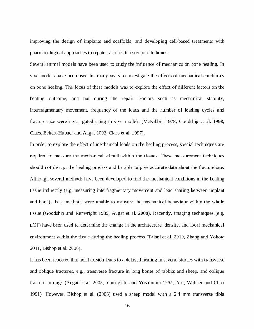
16

improving the design of implants and scaffolds, and developing cell-based treatments with

pharmacological approaches to repair fractures in osteoporotic bones.

Several animal models have been used to study the influence of mechanics on bone healing. In

vivo models have been used for many years to investigate the effects of mechanical conditions

on bone healing. The focus of these models was to explore the effect of different factors on the

healing outcome, and not during the repair. Factors such as mechanical stability,

interfragmentary movement, frequency of the loads and the number of loading cycles and

fracture size were investigated using in vivo models (McKibbin 1978, Goodship et al. 1998,

Claes, Eckert-Hubner and Augat 2003, Claes et al. 1997).

In order to explore the effect of mechanical loads on the healing process, special techniques are

required to measure the mechanical stimuli within the tissues. These measurement techniques

should not disrupt the healing process and be able to give accurate data about the fracture site.

Although several methods have been developed to find the mechanical conditions in the healing

tissue indirectly (e.g. measuring interfragmentary movement and load sharing between implant

and bone), these methods were unable to measure the mechanical behaviour within the whole

tissue (Goodship and Kenwright 1985, Augat et al. 2008). Recently, imaging techniques (e.g.

µCT) have been used to determine the change in the architecture, density, and local mechanical

environment within the tissue during the healing process (Taiani et al. 2010, Zhang and Yokota

2011, Bishop et al. 2006).

It has been reported that axial torsion leads to a delayed healing in several studies with transverse

and oblique fractures, e.g., transverse fracture in long bones of rabbits and sheep, and oblique

fracture in dogs (Augat et al. 2003, Yamagishi and Yoshimura 1955, Aro, Wahner and Chao

1991). However, Bishop et al. (2006) used a sheep model with a 2.4 mm transverse tibia

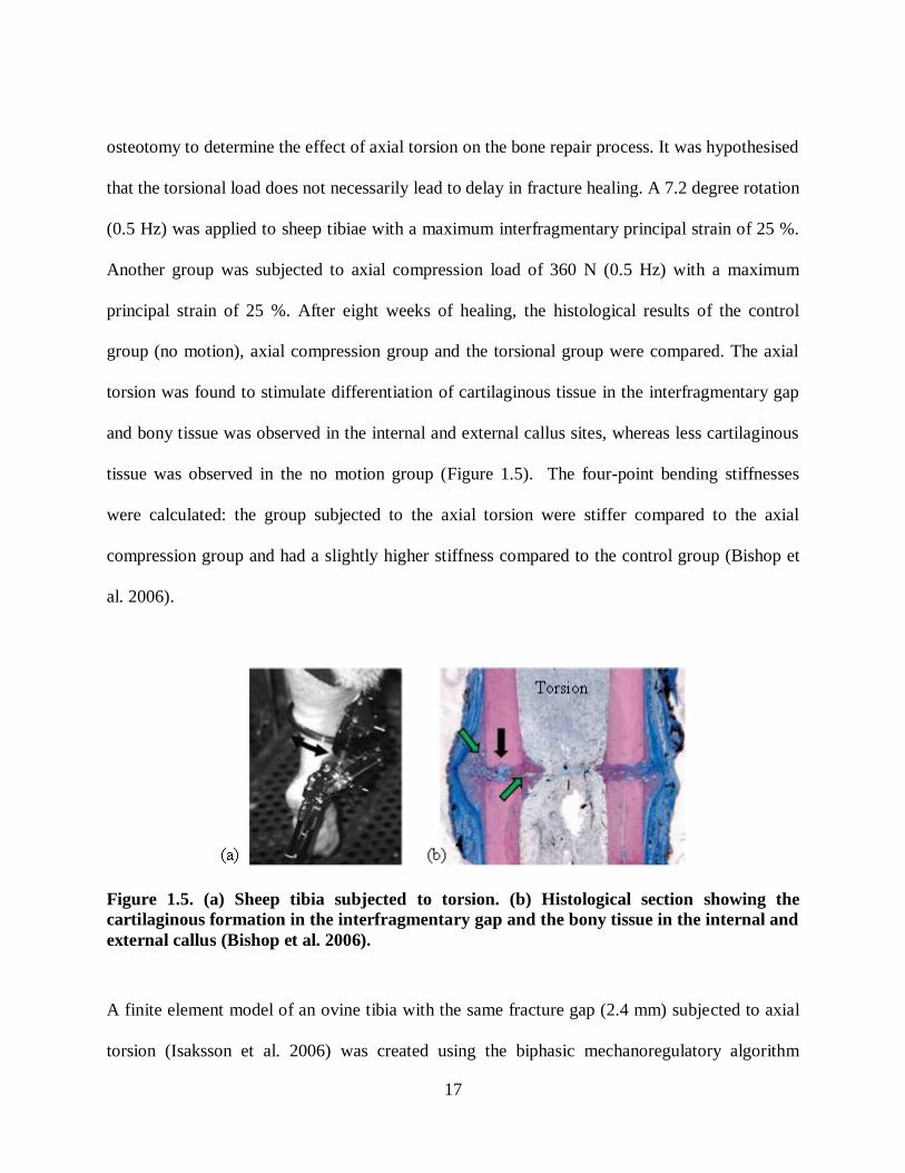
17

osteotomy to determine the effect of axial torsion on the bone repair process. It was hypothesised

that the torsional load does not necessarily lead to delay in fracture healing. A 7.2 degree rotation

(0.5 Hz) was applied to sheep tibiae with a maximum interfragmentary principal strain of 25 %.

Another group was subjected to axial compression load of 360 N (0.5 Hz) with a maximum

principal strain of 25 %. After eight weeks of healing, the histological results of the control

group (no motion), axial compression group and the torsional group were compared. The axial

torsion was found to stimulate differentiation of cartilaginous tissue in the interfragmentary gap

and bony tissue was observed in the internal and external callus sites, whereas less cartilaginous

tissue was observed in the no motion group (Figure 1.5). The four-point bending stiffnesses

were calculated: the group subjected to the axial torsion were stiffer compared to the axial

compression group and had a slightly higher stiffness compared to the control group (Bishop et

al. 2006).

Figure 1.5. (a) Sheep tibia subjected to torsion. (b) Histological section showing the

cartilaginous formation in the interfragmentary gap and the bony tissue in the internal and

external callus (Bishop et al. 2006).

A finite element model of an ovine tibia with the same fracture gap (2.4 mm) subjected to axial

torsion (Isaksson et al. 2006) was created using the biphasic mechanoregulatory algorithm

18

proposed by Prendergast et al. (1997). The model's predictions were compared to the

experimental observations. The algorithm was able to predict the gap bridging, and the healing

patterns were close to the in vivo results (Bishop et al. 2006). In another in vivo study, the effect

of lateral loading on the healing rate of the open wounds was investigated. It was hypothesised

that the cyclic lateral loading may lead to accelerated wound closure. The 0.5 mm diameter

wounds were generated surgically in the left and right femur necks. The load was applied for

three minutes per day for three consecutive days to the left knee, while the surgical holes in the

right femurs were used as control (no motion). Comparing the results, the healing process was

accelerated throughout the femur, especially in the femoral midshaft and neck compared to the

control group (Figure 1.6). According to peripheral quantitative computed tomography (pQCT)

images, the mineral density was increased in the loading group (Zhang and Yokota 2011). The

mechanical testing revealed that the stiffness of the femur increased by mechanical loading. It

was concluded that knee loading could lead to faster healing in surgical wounds in the femur

neck and midshaft. Developing a loading device for human use to load the knee laterally may

help to reduce the risk of fracture and lead to enhanced healing. However, the load magnitudes

and proper loading conditions should be investigated for human use.

Taiani et al. (2010) investigated a burr-hole fracture murine model treated with embryonic stem

cells implanted in a collagen scaffold at the fracture site. A 0.7 mm burr-hole fracture, with a

depth of 1.07±0.21 mm, was drilled through the medial cortex and the medullary cavity of the

proximal tibia. The centre of the hole below the top of the epiphysis was 2.49±0.26 mm (Taiani

et al. 2010). The burr-hole fracture was filled with collagenous scaffolds seeded with embryonic

stem cells, and the mice were allowed to move immediately after surgery. During 4 weeks of

healing µCT imaging was used to track the healing progress. There was enhanced recovery

19

observed at the fracture site with stem cell seeded scaffolds compared with controls, and an

increase in trabecular number and trabecular bone volume (Figure 1.7) (Taiani 2012).

1 week 2 weeks 3 weeks

(c)

(a) (b)

Knee loading

Figure 1.6. (a) Lateral loading of the left knee, (b) µCT images of burr-holes in control

group with delayed healing, and (c) loaded group with promoted healing. Bar = 1 mm

(Zhang and Yokota 2011).

Day 0 1 week 2 weeks 4 weeks

(b)

(a)

Figure 1.7. µCT images demonstrating the healing process and bone regeneration during 4

weeks: (a) in the control group, (b) collagenous scaffold seeded with ES cell-derived

osteoblasts implanted into the fracture site (Taiani 2012). Bar = 1 mm.

There are a tremendous number of variables involved in experimental investigations of bone

mechanobiology (e.g., the type of mechanical load, frequency, material properties of the scaffold

20

and pore size) that make them expensive, complicated and time consuming. As a result,

computational algorithms of mechanobiological processes have become an essential tool to

determine the mechanical environment within the tissues without disturbing the healing process

(e.g. stress, strain, fluid velocity) and develop a more complete understanding of the mechanical

factors involved in fracture healing. Mechanoregulatory algorithms quantitatively relate the

mechanical stimuli with the tissue behaviour using in vivo and in vitro data (Prendergast et al.

1997, Sandino and Lacroix 2011, Claes and Heigele 1999). Hence, both experimental and

computational models are essential to develop more realistic and sophisticated computational

models.

The following steps are required to develop computational models: (1) geometric reconstruction

of the in vivo model, (2) application of the in vivo loads and boundary conditions, (3)

determination of the material properties of the tissues using histological techniques, fluorescent

labelling and µCT imaging, and (4) model validation against in vivo models of fracture healing

using µCT imaging, mechanical testing and histological slides (Epari et al. 2006, Lienau et al.

2005, Claes and Heigele 1999, Smith-Adaline et al. 2004). Figure 1.8 shows how computational

and experimental studies can be used to develop a mechanoregulatory model.

Some of the proposed algorithms considered soft tissues as single-phase (solid) linear elastic

materials and neglected the effect of the interstitial fluid. These algorithms were regulated by

strain and hydrostatic pressure or just the deviatoric strain (Carter and Wong 1988, Carter,

Blenman and Beaupre 1988, Claes and Heigele 1999). These algorithms could not predict the

bone healing pattern when bone was subjected to axial torsion (Isaksson et al. 2006). Due to the

biphasic nature of soft tissues, considering the effect of fluid flow makes the models more

21

realistic. Using poroelastic analysis, the mechanical stimuli such as fluid velocity, fluid

pressurization, and tissue stress and strain can be explored over time within the tissue.

Several biphasic algorithms were later proposed. As an example, the algorithm proposed by

Prendergast et al. (1997) was based on the interstitial fluid velocity and octahedral shear strain.

Unlike the single phase algorithms, this theory predicted the bone healing patterns under axial

torsion (Isaksson et al. 2006). This theory has two constants that weigh the relative sensitivities

for octahedral shear strain and fluid velocity. These empirical constants do not have a physical

meaning and were obtained from trial and error comparisons of model predictions for fracture

healing patterns with in vivo observations. The complexity of biological events makes the use of

trial-and-error methods qualitative at best without a rigorous basis to constants used in the

models.

In addition to the mechanical behaviour, some cellular activities, such as cell proliferation,

apoptosis, callus growth and angiogenesis have been modelled (Sandino and Lacroix 2011,

Isaksson et al. 2008, Prendergast et al. 1997). However, in biological models there are various

simplifying assumptions which should be further developed. For example, the cell migration

rates are not well known and are estimations or obtained from experimental data from other

species. Further, the computational studies need validation against experimental data. Most of

the time, the experiments have not been performed by the same group and the boundary

conditions and mechanical loads applied to the model are not exactly known.

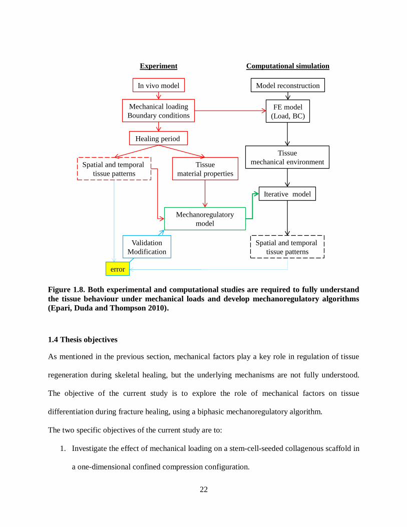
22

In vivo model

Mechanical loading

Boundary conditions

Healing period

Spatial and temporal

tissue patterns

Tissue

material properties

Model reconstruction

Computational simulationExperiment

FE model

(Load, BC)

Tissue

mechanical environment

Mechanoregulatory

model

Iterative model

Spatial and temporal

tissue patterns

error

Validation

Modification

Figure 1.8. Both experimental and computational studies are required to fully understand

the tissue behaviour under mechanical loads and develop mechanoregulatory algorithms

(Epari, Duda and Thompson 2010).

1.4 Thesis objectives

As mentioned in the previous section, mechanical factors play a key role in regulation of tissue

regeneration during skeletal healing, but the underlying mechanisms are not fully understood.

The objective of the current study is to explore the role of mechanical factors on tissue

differentiation during fracture healing, using a biphasic mechanoregulatory algorithm.

The two specific objectives of the current study are to:

1. Investigate the effect of mechanical loading on a stem-cell-seeded collagenous scaffold in

a one-dimensional confined compression configuration.

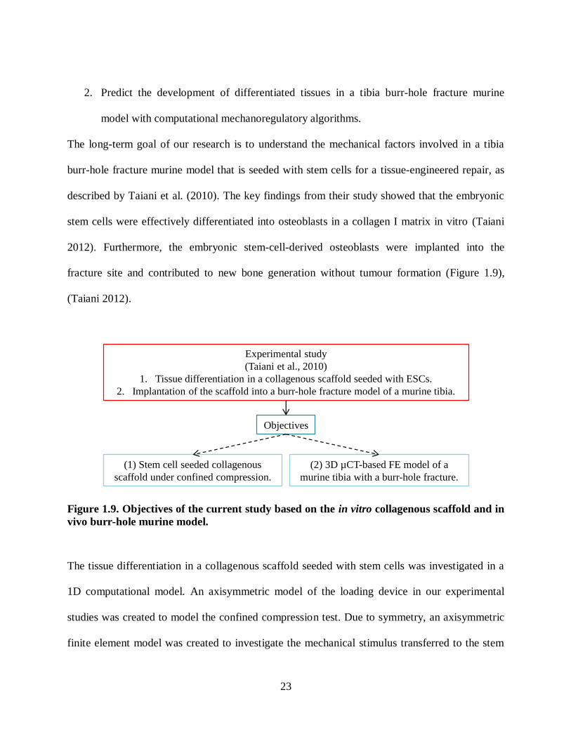
23

2. Predict the development of differentiated tissues in a tibia burr-hole fracture murine

model with computational mechanoregulatory algorithms.

The long-term goal of our research is to understand the mechanical factors involved in a tibia

burr-hole fracture murine model that is seeded with stem cells for a tissue-engineered repair, as

described by Taiani et al. (2010). The key findings from their study showed that the embryonic

stem cells were effectively differentiated into osteoblasts in a collagen I matrix in vitro (Taiani

2012). Furthermore, the embryonic stem-cell-derived osteoblasts were implanted into the

fracture site and contributed to new bone generation without tumour formation (Figure 1.9),

(Taiani 2012).

Experimental study

(Taiani et al., 2010)

1. Tissue differentiation in a collagenous scaffold seeded with ESCs.

2. Implantation of the scaffold into a burr-hole fracture model of a murine tibia.

(1) Stem cell seeded collagenous

scaffold under confined compression.

Objectives

(2) 3D µCT-based FE model of a

murine tibia with a burr-hole fracture.

Figure 1.9. Objectives of the current study based on the in vitro collagenous scaffold and in

vivo burr-hole murine model.

The tissue differentiation in a collagenous scaffold seeded with stem cells was investigated in a

1D computational model. An axisymmetric model of the loading device in our experimental

studies was created to model the confined compression test. Due to symmetry, an axisymmetric

finite element model was created to investigate the mechanical stimulus transferred to the stem

24

cell seeded gel. A poroelastic analysis was performed to consider the effect of interstitial fluid

within the scaffold. Since the boundary and loading conditions acting on the scaffold may also

play a crucial role in the differentiation process, the collagenous scaffold was subjected to

different magnitudes of pressure (20 kPa, 5 kPa, 1 Hz). The load transfer from the system to the

collagenous gel was investigated, and the distribution of mechanical stimuli was determined

within the solid and fluid phases of the gel. The predicted values of strain and fluid velocity

within the scaffold were found to be negligible in the 5 kPa (1Hz) case compared to the 20 kPa

(1Hz) case. Therefore, 20 kPa pressure was expected to stimulate the cells better and induce

appropriate biophysical stimuli to the scaffold compared to the 5 kPa (1Hz) case. Thus, a

biphasic mechanoregulatory algorithm was used to predict the tissue differentiation within the

scaffold (20 kPa, 5 kPa, 1 Hz). It was hypothesised that the 5 kPa predict less activity within the

scaffold. As expected within the 20 kPa loading case the cell proliferation and differentiation

were augmented. Hence, the use of appropriate mechanical loading led to promoted

differentiation within the scaffold. The loaded collagenous gel may then be implanted into the

fracture site and contribute to an enhanced healing.

In the second part of the thesis, a stem-cell-seeded collagenous scaffold was implanted into the

fracture site of a murine tibia, to explore the effect of mechanical loading on tissue

differentiation. To determine more realistic knowledge about the mechanical environment within

the fracture gap, the actual geometry of the murine tibia was reconstructed from the µCT images.

The reconstructed FE model was based on the in vivo murine model used by Taiani et al. (2010).

The burr-hole defect and the constructed computational model are shown in Figure 1.10.

25

(c) (d)

2.49±0.26 mm

0.71±0.04 mm

(a) (b)

2.55 mm

0.70 mm

1.04±0.21 mm1. mm

Figure 1.10. Location of the burr-hole in the medial aspect of the tibia: (a)

reconstructed FE model based on the in vivo study, (b) µCT image of the in vivo model

(Taiani 2012). A section through the long axis of the burr-hole looking proximally: (c)

reconstructed FE model based on the in vivo study and (d) µCT image (Taiani 2012).

The transfer of mechanical load to a fracture site depends on the quality and structure of the

surrounding bone. Tissue formation in an osteoporotic bone with less strength and increased

porosity is compromised compared to healthy bone. Moreover, the sensitivity of the bone to

mechanical perturbations may have been reduced. However, it is not clear whether the reduced

bone sensitivity is due to a reduced cell number or cell sensitivity. Computational models can be

used to determine the mechanical environment within the fracture site and investigate the factors

that can best promote fracture healing.

26

In the current study, mechanoregulatory algorithms were used and the tissue formation was

predicted under different loading conditions. To simulate both biological and mechanical factors

during bone regeneration, an existing biphasic mechanoregulatory algorithm regulated by

octahedral shear strain and interstitial fluid velocity was implemented into our simulations

(Prendergast et al. 1997, Isaksson et al. 2006). To simulate the recruitment of progenitor cells, a

diffusion process coupled to the poroelastic stress analysis was developed and verified against

the work by Isaksson et al. (2006).

1.5 Thesis overview

The second chapter of the thesis reviews research on mechanoregulatory mechanisms of bone

repair. The general goal of these studies was to investigate the effect of mechanical loading

driving stem cells to differentiate in a fracture. Chapter 2 of the thesis presents a general

description of the principal bone mechanoregulatory theories. The computational simulations

that have been developed and their applications in bone tissue engineering are discussed. Chapter

3 opens with an overview of bone mechanics and soft tissue biphasic theory that is used in

computational mechanoregulatory models. Next, the development and validation of the

implemented mechanoregulatory algorithm are described. The validated algorithm was

implemented into two idealised murine models and the effects of mechanical loading on the

healing process were investigated. In chapter 4, the simulation of the loading device used to load

the stem cell seeded scaffold is explained, and the effect of confined compression was explored

on tissue differentiation. Chapter 5, the reconstruction of murine tibia from µCT images is

discussed, and then a collagenous scaffold seeded with stem cells were implanted into the

fracture site. Using a biphasic mechanoregulatory algorithm the effect of mechanical stimulation

27

was determined in the burr-hole fracture murine model. Chapter 6, summarises the conclusions

and discuss the limitations of the current study and future prospects.

28

Chapter Two: Mechanoregulation Algorithms of Tissue Differentiation in Bone

It is known that mechanical factors can influence the biological synthetic processes in a variety

of tissues, which commonly referred to as mechanobiology. Biological tissues and particularly

those with a mechanical function, e.g. bone, are mechanosensitive, and can optimise their

material properties to different physical conditions (Sandino and Lacroix 2011, Palomares et al.

2009). Mechanical loads significantly affect all stages of tissue regeneration during skeletal

healing, however, it is not fully understood how tissue regeneration can be affected by

mechanical conditions. A number of different mechanoregulation algorithms have been

developed based on empirical comparisons of tissue differentiation patterns observed under

different loading regimes. In the first two sections, the first proposed mechanoregulatory

algorithms are outlined. In the third section, the mechanostat theory and the relationship between

tissue strain levels, and bone modelling and remodelling is presented. Finally, the algorithms

used in the computational simulations to model bone repair are discussed (Figure 2.1). These

algorithms can be broken into: single-phase models, biphasic models, and models with biological

factors.

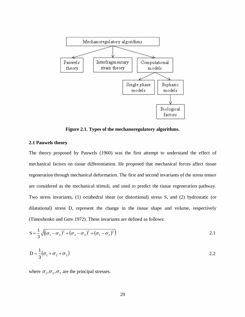
29

Figure 2.1. Types of the mechanoregulatory algorithms.

2.1 Pauwels theory

The theory proposed by Pauwels (1960) was the first attempt to understand the effect of

mechanical factors on tissue differentiation. He proposed that mechanical forces affect tissue

regeneration through mechanical deformation. The first and second invariants of the stress tensor

are considered as the mechanical stimuli, and used to predict the tissue regeneration pathway.

Two stress invariants, (1) octahedral shear (or distortional) stress S, and (2) hydrostatic (or

dilatational) stress D, represent the change in the tissue shape and volume, respectively

(Timoshenko and Gere 1972). These invariants are defined as follows:

2

31

2

32

2

213

1S 2.1

3213

1D 2.2

where 321 ,, are the principal stresses.

30

The octahedral shear stress deforms the material without inducing any change in its volume (i.e.

it causes octahedral shear strain). On the other hand, when the material is subjected to

hydrostatic stress, there will be a volumetric change without causing any distortion (i.e. it causes

pure volumetric strain).

Combining histological findings and mechanical theories, Pauwels (1960) concluded that the

elongation of extra cellular matrix without any volume change, caused by octahedral shear stress,

promotes collagenous formation. However, a volumetric change in the extracellular matrix

(caused by a hydrostatic stress) will enhance differentiation of cartilaginous tissue. A

combination of volumetric change and distortion within the extracellular matrix will lead to

regeneration of fibrous tissue. Pauwels (1960) believed that bone formation would not be

initiated unless there is a stable mechanical environment (Figure 2.2). The damaged bone

stabilises the environment by formation of fibrous and cartilaginous tissue. Therefore, after

formation of fibrous and cartilaginous tissue, the bony tissue starts to differentiate (Pauwels

1960, Lacroix 2000).

Figure 2.2. A schematic of Pauwels' theory, octahedral shear stress and hydrostatic

pressure used as biophysical stimuli (Pauwels 1960).

31

2.2 Interfragmentary strain theory

The interfragmentary strain theory was developed by (Perren 1979, Tubbs 1981). They suggested

that each tissue type has a specific strength and strain tolerance. In other words, different types of

tissues can absorb different levels of strain. A detailed knowledge of the strain within the callus

would enable the prediction of tissue differentiation. For instance, granulation tissue can stretch

approximately 100 % before rupture, whereas cartilage tolerates strains up to 10 % only, and

bone would fail under strains greater than 2 % (Figure 2.3). Hence, if the strain within the tissue

were more than 2 %, differentiation and maintenance of a bony tissue would not be possible

according to this theory. The healing of bone initiates from the differentiation of tissues with the

highest tolerance to strain (granulation tissue) and continues to cartilage and bony tissue due to

the differences in strain that can be tolerated by these tissues (Figure 2.3).

The interfragmentary strain is the interfragmentary motion divided by the fracture gap size when

bone is considered as a one dimensional (1D) object. Although the movement of the fracture gap

can easily be measured, the interfragmentary theory has two main drawbacks. First, bone fracture

is three-dimensional (3D) and is only being modelled as a 1D problem. Second, the

interfragmentary theory predicts enhanced healing in the fractures with larger gap size. However,

this is in contrast with experimental observations (Claes et al. 1997, Augat et al. 1998).

Figure 2.3. Strain tolerance of different types of tissues (Tubbs 1981).

32

2.3 Mechanostat theory, (Frost, 1987)

The changes in bone such as three longitudinal growth, bone modelling and bone remodelling

are always controlled by a mechanism called mechanostat (Frost, 1987). The mechanism should

check the efficiency of the bone itself, the mechanism that transforms the mechanical signal to

the bone and the sensors that are responsible to sense the signal resulting from the applied

mechanical loads. The strains applied to the bone, depending on their magnitude, may lead to

bone modelling or remodelling. During the modelling process the mass density of the cortical

bone increases; whereas during the bone remodelling the existing cortical endosteal and

trabecular bone is absorbed in some regions and will be replaced by new bony tissue. The bone

modelling and remodelling process will automatically start when strains deviate from certain

setpoints. These strain setpoints change if the responsible agents for sensing or transmitting the

mechanical load to the bone are damaged (e.g. postmenopausal, osteoporosis and osteogenesis

imperfecta). Diseases affect the sensitivity of the cells and make them insensitive or over-active

(Frost, 1987).

A number of set points have been identified to describe bone behaviour: (1) minimum effective

strain (MES), (2) the strain range that lead to bone loss due to an imbalance in the remodelling

process and bone resorption outpaces bone formation ([0,MESr]), (3) the strain higher than this

setpoint lead to bone modelling and bone will be added to surfaces (MESm), (4) the strains

higher than a special setpoint that damaged bone and bone repair should initiate (MESp), and (5)

the bone fracture strength (Fx), (Figure 2.4). When bone is subjected to strains lower than MESm

it is known to be in a homoeostatic state in which bone remodelling is in equilibrium (AW,

adapted window). There is a balance between bone resorption and formation (dead zone or lazy

zone), and there is no net change in bone mass. If bone is under a mild over load (MOW, mild

33

over load window), the bone formation outpaces bone resorption. In case of higher rates of

strain, where micro-damage occurs woven bone formation initiates (POW, pathological overload

window), (Figure2.4).

When the bone is not in the lazy zone, the bone cells will be activated and the bone formation

and absorption will continue until they reach to the homeostatic state. Frost compared this

mechanism with a thermostat, in which the preset temperatures are like the setpoints in a bone. In

case of an increase or a decrease in room temperature, the system will work to raise the

temperature back to its target value.

MES MESm MESp Fx

AW MOW POW

remodelling

lamellar drifts

woven bone drifts

Form

atio

nR

esorp

tion

Figure 2.4. Graph shows the mechanostat theory proposed by Frost (Frost, 2003). The

relationship between the tissue strain level and change in bone mass is presented. AW,

MOW and POW refer to the dead zone, mild overload and excessive load, respectively.

MESm and MESp are the bone modelling and the micro-damage thresholds, respectively.

Fx is the bone fracture strength. These setpoints vary between individuals and are

hypothesised to be genetically determined.

34

2.4 Computational simulations of tissue differentiation

2.4.1 Single solid phase model (Carter’s theory, 1988)

Carter et al. (1988) proposed a mechanoregulation theory based on the octahedral shear stress

and hydrostatic (or dilatational) stress (Carter et al. 1988, Carter and Wong 1988). It was the first

time that finite element analysis (FEA) was used to make quantitative predictions of tissue

differentiation. In this algorithm, bone was considered as a linear elastic single phase material

(solid). Equation 2.3 was used to predict tissue differentiation:

kDSI 2.3

where I was defined as the “osteogeni index” representing the tendency for ossification, S was

the octahedral shear stress, D was the hydrostatic stress, and k was an empirical constant to be

determined.

High values for I represented bony tissue differentiation and accelerated ossification, whereas

low values predicted artilaginous tissue differentiation. ased on Carter‟s theory, fi rous tissue

differentiation occurred in areas subjected to high levels of shear stress. On the other hand,

cartilage differentiation occurred in areas under high hydrostatic compressive stress and low

amount of shear stress. Good vascularity, low shear and high hydrostatic stress stimulate bone

formation. It was found that in areas under low shear and hydrostatic stress levels along with

poor vascularity, there would be no bone formation and only cartilage would differentiate

(Figure 2.5).

The model was further modified to consider the number of load cycles (n) to simulate tissue

differentiation and gradual change of tissue strength (Figure 2.6). The obtained equation is

shown as follows (Carter and Wong 1988):

35

c

i 1

iii kDSnI , c1,2,...,i . 2.4

where in showed the number of loading cycles, and i was the discrete loading conditions, k was

an experimental constant.

A two-dimensional FE model of a femoral midshaft rabbit osteotomy with an external callus was

created. The model was subjected to axial and bending loads. The octahedral shear stress and the

hydrostatic stress were calculated from the computational analysis. Different values of k (0, 0.5.

1, 2) were used to find the osteogenic index (I). Depending on the obtained values of I, contour

plots of the osteogenic index were used to predict areas of endochondral ossification (higher

values of I) and cartilaginous formation (lower I values). The contours were then compared with

the available histological slides. The best match was found using the value of 2 for k. Another

computational study was performed to predict the tissue patterns in an idealised long bone and

the proximal femur. However, comparing the numerical results with the available histological

slides, it was concluded that k could vary between 0.3 and 1. Therefore, for each simulation

different values of k were used to predict tissue patterns (Carter, Wong and Orr 1991).

Carter et al. (1998) proposed another theory which was based on tensile strain and hydrostatic

stress, (Figure 2.6). According to the modified algorithm: (1) low hydrostatic stress and tensile

strain promote direct intramembranous ossification, (2) high tensile strain and hydrostatic

compressive stress stimulate the formation of fibrocartilage, (3) high tensile strain promotes the

development of fibrous tissue, and (4) hydrostatic compressive stress is the stimulus for

cartilaginous tissue differentiation.

An axisymmetric FE model of a long bone fracture was created. The cortical bone was modelled

as a rigid body and other tissues (e.g. fibrous tissue, cartilage and bone) were assumed to be

36

linearly elastic and isotropic. The axial compressive load was applied to the cortical shaft. The

patterns of tensile strain and hydrostatic stress were determined at the fracture site. It was

concluded that bone formation occurs in the areas that cartilage tissue existed. Bone formation

might be delayed by intermittent hydrostatic compressive stress and can be promoted by tensile

strain (Carter and Wong 1988).

Bone is a biphasic material consisting of a solid and fluid phase with viscoelastic properties.

However, both soft and bony tissues were modelled as a single phase, linearly elastic material in

Carter‟s algorithm. Hen e, this model may not e a le to fully apture and explain the tissue

differentiation processes.

Figure 2.5. The effect of mechanical loading and vascularity on bone differentiation (Carter

et al. 1988).

37

Figure 2.6. Carter's mechanobiology theory. Principal tensile strain and hydrostatic stress

history are the key biophysical stimuli n p 2001).

2.4.2 Single solid phase model (Claes and Heigele, 1999)

Claes and Heigele introduced a new hypothesis, which relates the local tissue formation in a

fracture gap to the local stress and strain (Claes and Heigele 1999). An axisymmetric FE model

of a sheep fracture with external callus was used to calculate stresses and strains in the callus.

The initial connective tissue was modelled as a hyperelastic material and other parts (e.g. soft,

intermediate, and stiff callus, ossification and cortex) were considered linear elastic.

It was believed that cartilage forms in regions experiencing excessive hydrostatic compressive

stress; fi rous tissue differentiates under high tensile strain levels and fi ro artilage forms from a

combination of hydrostatic pressure and tensile strain (Claes and Heigele 1999). The proposed

algorithm by Claes et al. (1999) is similar to the one proposed by Carter et al. (1988) are similar.

It was the first time that the thresholds were quantified to predict what tissue would form. Figure

2.7 illustrates the rule of tissue differentiation relating mechanical stimuli to the tissue types as

hypothesized by Claes and Heigele (1999).

38

Figure 2.7. Single phase model introduced by Claes et al. (1999) in which hydrostatic

pressure and strain are the key biophysical stimuli.

2.4.3 Single solid phase model (Gardner et al., 2000)

A 2D FE model based on orthogonal radiographs of a diaphyseal tibial fracture was created to

find the maximum principal stress at four critical stages of the bone healing process (Gardner et

al. 2000). The callus was divided into different regions representing different types of tissues.

The material properties were defined based on the tissues observed in histological slides and

updated before each healing stage. The tissue patterns were correlated with the stress and strain

distributions. It was hypothesized that high levels of principal stress may decrease the tissue

stability and delay the healing process. The maximum strain in the interfragmentary gap was

computed during the healing process. According to the results, the strain decreased from 70 % to

2 % during two months of repair. Since the material properties used during the analysis were

based on tissues observed in the histological slides, the predicted stress and strain patterns were

more accurate when compared to previous algorithms. However, the data was obtained from

only one patient and no comparisons were done using other patients. Furthermore, the complex

3D fracture was modelled in 2D, which may decrease the quantitative predictions of the

simulation.

39

2.4.4 Biphasic model (Kuiper et al., 1996-2000)

In 1996, Kuiper et al. created an axisymmetric model of human bone. The tissues were

considered as biphasic materials, composed of solid and fluid phases, to incorporate the effect of

the interstitial fluid movement. The fluid shear strain and shear stress were used as biophysical

stimuli to drive tissue differentiation. Moreover, bone resorption was also predicted using the

strain energy (Kuiper et al. 1996, Kuiper et al. 2000a, Kuiper et al. 2000b). The mass turnover

was determined as follows:

refS

ρ

Uρθa

dt

dρ 2.5

where θ is a time constant, ρa is the internal free surface per unit volume, U denotes the

tissue level strain energy, ρ is the apparent density and refS is a reference value of ρ

U . The

strain energy density would be:

σε 2

1U 2.6

where ε is the strain tensor and σ is the stress tensor. Resorption ( 0dt

dρ ) would occur if

refref Ss1ρ

USs1 and 0.35s (Van Rietbergen et al. 1993).

Kuiper et al. (2000) deduced that in a fracture callus, strain plays an important role to stimulate

tissue differentiation. Fluid shear stress (τ) an e found using the Carman-Kozeny equation:

3

2

int ndl.dA

dAkGμ

2.7

40

where dl.dA

dAint is known as the specific surface (s), dA is the cross sectional area, intdA is the

internal surface, dl is the infinitesimal length, k is the tissue permeability; n is the porosity, µ is

the fluid viscosity, and G is a constant. Solution of this equation determines the specific surface s

and is then used to find the fluid shear stress τ:

s

pη

2.8

where

z

p,

y

p,

x

pp is the pressure gradient. A schematic of the algorithm is illustrated in

Figure 2.8. An axisymmetric model of a fracture callus under different compressive loads was

modelled to investigate the healing patterns. The cyclic loads were applied to the cortical bone.

According to the numerical study, the amount of fibrous tissue was increased in case of

increasing the magnitude or duration of movements. However, the healing was delayed by

increasing the magnitude of movements (Matsushita and Kurokawa 1998, Goodship and

Kenwright 1985).

Figure 2.8. Biphasic model introduced by Kuiper et al. (2000a), using fluid shear strain and

stress as the biophysical stimuli.

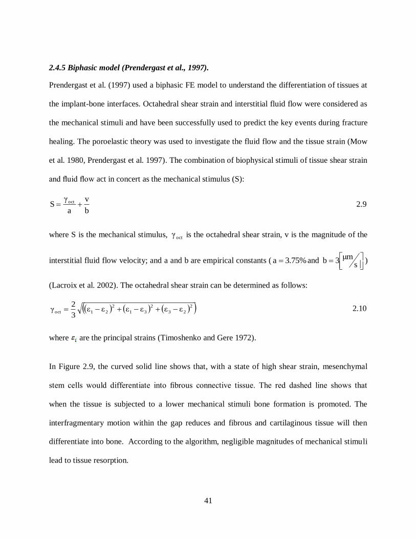
41

2.4.5 Biphasic model (Prendergast et al., 1997).

Prendergast et al. (1997) used a biphasic FE model to understand the differentiation of tissues at

the implant-bone interfaces. Octahedral shear strain and interstitial fluid flow were considered as

the mechanical stimuli and have been successfully used to predict the key events during fracture

healing. The poroelastic theory was used to investigate the fluid flow and the tissue strain (Mow

et al. 1980, Prendergast et al. 1997). The combination of biophysical stimuli of tissue shear strain

and fluid flow act in concert as the mechanical stimulus (S):

b

v

a

γS oct 2.9

where S is the mechanical stimulus, octγ is the octahedral shear strain, v is the magnitude of the

interstitial fluid flow velocity; and a and b are empirical constants ( 3.75%a and

sμm

3b )

(Lacroix et al. 2002). The octahedral shear strain can be determined as follows:

2

23

2

31

2

21oct εεεεεε3

2γ 2.10

where are the principal strains (Timoshenko and Gere 1972).

In Figure 2.9, the curved solid line shows that, with a state of high shear strain, mesenchymal

stem ells would differentiate into fi rous onne tive tissue. The red dashed line shows that

when the tissue is subjected to a lower mechanical stimuli bone formation is promoted. The

interfragmentary motion within the gap reduces and fibrous and cartilaginous tissue will then

differentiate into bone. According to the algorithm, negligible magnitudes of mechanical stimuli

lead to tissue resorption.

42

Figure 2.9. Proposed biphasic algorithm by Lacroix et al. (2002) in which octahedral shear

strain and fluid velocity are the biophysical stimuli.

Table 2.1. Mechanoregulatory stimulus for tissue differentiation (Prendergast et al. 1997).

Mechanoregulatory stimulus (S) Predicted tissue differentiation

S>3 fibrous connective tissue

3>S>1 chondrocytes and cartilage

1>S>0.267 osteoblasts & immature bone

0.267>S>0.01 mature bone & remodelling

S<0.011 Resorption

Depending on the loading conditions, various magnitudes for the mechanical stimulus, S, are

possible which can lead to fibrous tissue, immature and mature cartilage, and immature,

intermediate and mature bone differentiation (Lacroix et al. 2002). High values for S promote the

differentiation of mesenchymal stem cells into fibrous tissues 6S3 , intermediate values

stimulate cartilage differentiation 3S1 , and low levels lead to formation of immature

43

1S0.267 and mature bony tissue 0.267S0.011 . Different values for S representing

different types of tissues are shown in Table 2.1.

2.4.6 Biphasic model (Sandino and Lacroix, 2011)

Sandino and Lacroix (2011) made further modifications to the model introduced by Prendergast

et al. (1997). The purpose of their study was to explore the effect of mechanical perturbation and

perfusion flow on tissue differentiation in a calcium phosphate-based glass porous scaffold. The

octahedral shear stress within the tissue and the shear stress within the fluid (instead of fluid flow

velocity) were used as mechanical stimuli. The fluid shear stress was used instead of fluid

velocity to investigate the effect of fluid perfusion into a scaffold. The solid phase was modelled

as a linear elastic solid and the fluid phase was considered as a Newtonian fluid. In the fluid

model different levels of viscosity simulated tissue regeneration. In addition to the prediction of

tissue differentiation and resorption (e.g. fibrous, cartilaginous and bony tissue), the prediction of

cell death was also added to the algorithm proposed by Prendergast et al. (1997). The variation of

fluid shear stress was observed during the differentiation process. Sandino and Lacroix (2011)

concluded that the variations of fluid shear stress should be controlled in vivo to avoid a delay in

the formation of new tissues. The modified graph is illustrated in Figure 2.10. The

mechanoregulation index M can be represented by the equation:

b

η

a

γM oct 2.11

where octγ is the o tahedral shear strain, τ is the fluid shear stress, and a and b are the empirical

constants (a=0.0375, b=10 [MPa]). Different intervals for M representing different types of

tissues are shown in Table 2.2.

Fluid shear stresses were found using Newtonian fluid formulation:

44

2

0

0

02

0

0

02

vμη

21

31

32

2.12

where µ is the fluid viscosity,

zv,

yv,

xvv is the velocity gradient, and

1ζ and 3ζ

are the minimum and maximum principal fluid stresses, respectively.

Figure 2.10. Biphasic model introduced by Sandino and Lacroix (2011) in which fluid shear

stress and octahedral shear strain were used as biophysical stimuli.

Table 2.2. Biphasic model prediction of tissue differentiation by Sandino and Lacroix

(2011).

Mechanoregulatory stimulus (M) Predicted tissue differentiation

M>6 o τ<0.01 no tissue formation

3>M>6 fibrous tissue

1>M>3 Cartilage

1>M>0.001 Bone

45

2.4.7 Models with biological factors

There are many biological factors affecting the fracture healing process: proliferation, migration,

growth factors, tissue growth and cell modelling. Bailon-Plaza and van der Meulen (2001)

presented a purely biological algorithm to study the effect of osteogenic and chondrogenic

growth factors on fracture healing. Mechanical factors were not taken into consideration in this

model. Tissue differentiation was controlled by seven biological variables: concentration of

mesenchymal stem cells, chondrocytes, osteoblasts, osteogenic and chondrogenic growth factors

and the density of a om ined fi rous/ artilaginous extra ellular matrix or a one extra ellular

matrix. A finite difference method was used to solve a system of 2D partial differential equations

based on the presence of osteogenic and chondrogenic growth factors. The temporal tissue

regulation and cellular events were modelled using the finite difference method (Bailon-Plaza

and van der Meulen 2001). The numerical model predicted the distribution of different tissues

over time, the rate of osteogenic growth factor production by osteoblasts, and determined that the

duration of initial release of growth factors are important to have a successful healing and

ossification. The computational prediction of the time points of osteogenic growth factor

concentrations in callus were close to empirical evidence in the rat fracture callus (Joyce et al.

1990). Bailon-Plaza and van der Meulen (2003) further modified this algorithm by adding

mechanical factors to the model. In addition, Geris et al. (2006) used the bioregulatory model to

simulate a fracture healing process in a murine tibia and the computational results were

compared to experimental observations. The concentration of the growth factor over time was

compared with an experimental study done on murine fracture healing (Cho, Gerstenfeld and

Einhorn 2002). The chondrogenic growth factors were mainly observed in the first week of the

fracture and the osteogenic growth factors were observed in the second week of the healing

46

process (Cho et al. 2002, Geris et al. 2006). The major drawback with these models is that there

was no differen e etween the fi rous and artilaginous tissue components, and no distinction

etween fi roblasts and chondrocytes. Geris et al. (2008) further developed the model by adding

the angiogenesis aspect in bone fracture healing.

Another algorithm which models cell migration was proposed by Lacroix et al. (2002). In

general, cells have a random translational motion like the diffusion of the particles in a fluid or a

gas. They modelled cell proliferation and migration using a diffusion equation as an

approximation, which can be expressed as follows:

2

2

2

2

2

2

z

ρ

y

ρ

x

ρD

t

ρ 2.13

where ρ is the ell density and D is a diffusivity constant and is related to the cell proliferation

and migration rate. The migration, proliferation and cell differentiation is dependent on the

obtained cell density. The material properties were updated based on the average of computed

mechanical stimuli (fluid velocity and octahedral shear strain) in the previous 10 days and on the

temporal and spatial cell concentration:

updated

max

cellgran.

max

cellmaxfinal E

ρ

ρE

ρ

ρρE

2.14

where cell is the cell density obtained from equation 2.17, max is the maximum cell density,

updatedE is the Young‟s modulus o tained from equation 2.9 (Prendergast et al. 1997), updatedE is

the Young‟s modulus of the granulation tissue. The same equation was used to al ulate

permea ility and oisson‟s ratio.

47

The fracture healing stages in a human tibia were modelled by combining both cell migration,

and the biphasic algorithm proposed by Prendergast et al. (1997). A 2D axisymmetric FE of a

human tibia was modelled with a biphasic material description. The results were compared with

the patterns of the healing observed in vivo. The model successfully showed that the healing

process would be longer with larger fracture gaps. Moreover, the differentiation of fibrous tissue

was accelerated by applying higher levels of strain to the tibia in the early stages of fracture

repair (Lacroix et al. 2002). Later, this algorithm was used by Isakson et al. (2006) to model the

fracture healing process in an axisymmetric model of an ovine tibia. It was shown that the high

rates of mechanical stimuli increased the interfragmentary movement and delayed the bone

formation or lead to a non-union in the later stages of healing.

Garcia et al. (2007) developed the first mathematical model to explore the mechanical effects on

the callus size and geometry, and tissue differentiation. The model simulated different cellular

events during fracture healing: (1) mesenchymal stem cell migration, (2) proliferation, death and

differentiation, matrix synthesis, degradation, damage of mesenchymal, chondrocyte, fibroblast

and osteoblast, (3) calcification, and (4) remodelling over time (Garcia-Aznar et al. 2007).

Doblare et al. (2003) examined the tissue composition (collagen types, proteoglycans, mineral

and water) during the healing stages to determine the material properties and permeability of

different tissues (Doblare and Garcia 2003). The second invariant of the deviatoric strain tensor

( 2J ) was used as the mechanical stimulus:

22

2 tracetrace2

1J εε 2.15

where ε is the strain tensor.

48

The rate of change of the matrix volume was a linear function of cell density in each tissue. For

granulation, fibrous and cartilaginous tissue, and woven bone the formulation used is:

ii

i

matrix Qρt

V

2.16

where i indi ated the ell type, ρ is the ell density, Q is the matrix production per cell and unit

time, and the matrix production for lamellar bone was calculated as follows:

vrem

i

matrix Srkt

V

2.17

where

r was the formation/resorption of bone matrix volume per available bone surface per

time, vS was the specific bone surface and remk was the percentage of bone surface active for

remodelling.

According to their study, increases in gap movement increase the callus size (Doblare and Garcia

2003). The computational simulation for an axisymmetric sheep model was compared to the

interfragmentary motion in a sheep experiment (Claes et al. 1997). The callus shapes predicted

by their algorithm had a radial thickness approximately equal to the cortical thickness and had an

axial extension in both distal and proximal directions close to the radial thickness. These results

were in agreement with previous empirical studies that observed for healing osteotomies in

larger mammals (Claes et al. 1998, Goodship et al. 1998).

Another study in orporated a “random walk” or sto hasti model of ell migration with a latti e

modelling approach (Perez and Prendergast 2007). In this model, the cell migration was

modelled in two different ways: with and without preferred direction. An implant-bone interface

was investigated by this method and the results were compared with the diffusion model

49

proposed by Lacroix et al. (2002). Both models had very close predictions for the temporal

change of stiffness in the tissue differentiated within the gap. The only difference was that the

“random walk” ased model in the work by Perez and Prendergast (2007) showed greater

variation in the patterns of the differentiated tissues compared to the model proposed by Lacroix

et al. (2002). The diffusion process predicted continuous patterns of tissue differentiation,

whereas the random walk model had more heterogeneous tissue pattern. There were no

histological slides available to compare the diffusion and random walk models and show, which

best matched. However, the stochastic model had a more rapid reduction of the relative

displacement between the bone and implant (Perez and Prendergast 2007). Using the same

parameters resulted in different predictions of cell distribution, due to the random nature of the

stochastic model. This variation is comparable with experimental studies in cell histology.

Checa and Prendergast (2010) developed a model to incorporate both the mechanical

environment and an oxygen supply as regulators of cell differentiation. A mechanoregulatory

algorithm based on the fluid velocity and octahedral shear strain was used to predict tissue

differentiation inside the bone chamber inserted into a rat tibia using a poroelastic analysis

(Prendergast et al. 1997). The effect of angiogenesis in a scaffold with regular morphology was

also simulated. The computational model was able to mimic the growth and remodelling process

of the capillary network formation and investigate its effect on tissue differentiation. A lattice

approach was used to model cell migration, differentiation, proliferation, apoptosis and

angiogenesis were simulated. Each lattice point was either empty or occupied by a cell. Cell

activities were simulated by moving a cell from a lattice point to another (migration), dividing a

cell so that the daughter cell filled the neighbouring lattice point (proliferation), deleting a cell at

a lattice point (apoptosis), and the endothelial cells were linked to form capillaries within the

50

lattice (angiogenesis) (Prendergast, Checa and Lacroix 2010). The vessel growth was controlled

by a mechanoregulatory stimulus. The random walk theory (Perez and Prendergast 2007) was

implemented in the lattice approach to model cell migration. The mechanobiological algorithm

proposed by Prendergast et al. (1997) was used to consider the effect of mechanical loading on

MSCs differentiation and the effect of vascularity was added. As in the original Prendergast

algorithm, bone formation occurred when the mechanical stimuli was low. However, in the new

model (Checa and Prendergast 2009), the cell differentiation depended on the existence of a

nearby blood vessel. In the presence of oxygen, bone could differentiate, however, if blood

vessels were not available only cartilaginous tissues could differentiate (Figure 2.12). Probability

equations were used to simulate the growth direction and length of the blood vessels. The

formation of the vascular network was based on three events: (1) formation of vessel sprouts

from existing vessels or sprouts, (2) the growth of sprouts, and (3) merging a sprout tip to

another sprout tip or sprout. The path of the endothelial cell at the capillary tip determined the

direction of capillary. The endothelial path was itself determined using the random walk theory.

The sprout branching was a function of sprout length, and the rate of sprout growth was a

function of mechanical stimuli (fluid velocity and octahedral shear strain) (Figure 2.11). The

governing equations depend on both mechanical factors and the existence of vascular endothelial

growth factor (VEGF). VEGF stimulates the development of new blood vessels. In the

computational study by Checa and Prendergast (2009), the vessels reached the core of the

scaffold in six days, and after the first week, the rate of vessel growth decreased which is in

agreement with experimental data of Mikos et al. (1993). Predictions based on the model

indicated that higher mechanical loads caused slower formation of a capillary network and led to

a slower bony tissue differentiation (Checa and Prendergast 2010, Checa and Prendergast 2009).

51

Pro

bab

ilit

y b

ran

chin

g

Sprout lengthL(min) L(max)

maxΔL

Rat

e o

f gro

wth

Mechanical stimulus (S)

maxS

1

(a) (b)

Figure 2.11. (a) The relationship between the sprout branching and the sprout length, (b)

the rate of sprout growth as a function of mechanical stimulus (Checa and Prendergast

2009).

Figure 2.12. Mechanoregulatory algorithm proposed by Checa and Prendergast (2009)

simulating tissue differentiation by both the local mechanical environment and the

presence of oxygen from nearby blood vessels.

Isaksson et al. (2008) developed an algorithm that directly coupled mechanical stimuli to cellular

events. Two separate FE models of the mechanical environment in the tissues and a cell model

ran in parallel and data from one model was used to provide key driving factors to the other. The

cellular activities and tissue differentiation depended on the mechanical stimuli predicted

(deviatoric shear strain and fluid velocity). The mechanical stimuli were determined using the

52

Prendergast et al. (1997) algorithm. The cells acted as transducers during tissue differentiation.

In other words, the activities of each cell (mesenchymal stem cells, fibroblasts, chondrocytes or

osteoblasts) were based on the obtained mechanical stimuli and the activities of other cell types.

Each cell type either migrated, proliferated, differentiated or apoptosed. The effects of growth

factors were also implicitly modelled in the cell activities. The cell proliferation was assumed to

decrease linearly with cell density as the space was occupied and there was lack of nutritional

resources. The rate of cell migration was different for each cell type: mesenchymal stem cells

and fibroblasts had high rates, whereas chondrocyte and osteoblasts had low rates. The migration

was modelled using a diffusion analysis, where the migration was controlled by temporal cell

concentration.

The potential of the model was evaluated in a 2-D FE study of a human long bone osteotomy.

Comparing the computational results with the empirical observations showed that the model

predicted several aspects of bone healing such as cell and tissue distributions during fracture

repair, the effects of excessive mechanical perturbations on the healing process, e.g., periosteal

stripping and impaired effects of cartilage remodelling (Figure 2.13).

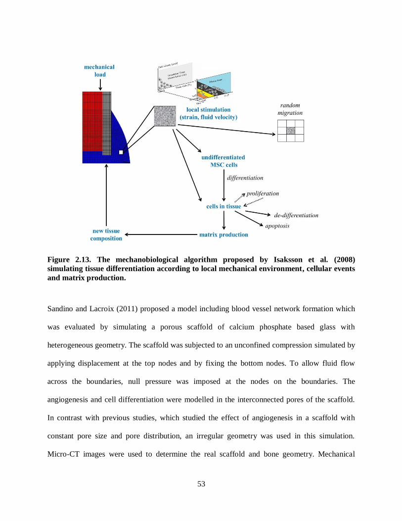
53

Figure 2.13. The mechanobiological algorithm proposed by Isaksson et al. (2008)

simulating tissue differentiation according to local mechanical environment, cellular events

and matrix production.

Sandino and Lacroix (2011) proposed a model including blood vessel network formation which

was evaluated by simulating a porous scaffold of calcium phosphate based glass with

heterogeneous geometry. The scaffold was subjected to an unconfined compression simulated by

applying displacement at the top nodes and by fixing the bottom nodes. To allow fluid flow

across the boundaries, null pressure was imposed at the nodes on the boundaries. The

angiogenesis and cell differentiation were modelled in the interconnected pores of the scaffold.

In contrast with previous studies, which studied the effect of angiogenesis in a scaffold with

constant pore size and pore distribution, an irregular geometry was used in this simulation.

Micro-CT images were used to determine the real scaffold and bone geometry. Mechanical

54

stimuli values were determined using the algorithm proposed by Prendergast et al. (1997).

Cellular activities including proliferation, migration, differentiation and MSCs and endothelial

cell initialization were modelled using a lattice approach. The MSCs attached to the wall of the

scaffold at the beginning of the simulation, and then started to move randomly. Each lattice point

had a probability, p, for locating a cell. The endothelial cells were assumed to be outside of the

interconnected pores and the empty lattice points had the probability of 0.1 to locate an

endothelial cell. An event could occur with the probability of p, and could not occur with the

probability of (1-p). The probability was based on the mechanical stimulus, S in the lattice point.

Blood vessels were represented by linking the endothelial cell within the neighbouring lattice

points. The angiogenesis simulation was based on two main factors: (1) modelling the direction

and the rate of growth of each vessel, and (2) its probability of branching. Three approaches were

used to study the growth direction: (1) a random direction, (2) the primary direction used in the

whole analysis, and (3) the direction was set toward regions with higher VEGF concentration.

The vessel growth rate depended on the mechanical stimulus at the beginning of the blood

vessel. Vessel branching was determined according to its length. Tissue differentiation was

predicted based on the combination of both mechanical stimulus and the vessel network

formation. Different types of tissues were predicted within the scaffold subjected to unconfined

strain; however, osteogenesis was not predicted in most of the pores at the center of the scaffold.

Such understanding of tissue differentiation based on angiogenesis and mechanical stimulus

might lead to better scaffold developments. A schematic of the proposed algorithm is shown in

Figure 2.14.

55

Figure 2.14. Mechanoregulatory algorithm proposed by Sandino and Lacroix (2011)

simulating tissue differentiation based on mechanical stimuli, cellular events and

angiogenesis.

Nagel and Kelly (2010) extended the algorithm proposed by Prendergast et al. (1997) to

investigate the effects of mechanical loading on collagen fibre directions and tissue

differentiation. An anisotropic biphasic material model was used to simulate an idealised rat

femur fracture model subjected to cyclic bending. The mechanical stimulus was based on fluid

velocity and octahedral shear strain. Cell migration and proliferation were modelled using a mass

diffusion equation. Angiogenesis and the effect of growth factors, or any other biological factors,

were not modelled. The material properties were updated based on the average of computed

mechanical stimuli in the previous 10 steps (days) and on the temporal, cell concentration as well

as the fibre orientations.

Fibre directions were updated according to the predicted unit vectors ( ia ,0 , ig ,0 ) from the last ten

days. The unit vectors represented the preferred fibre directions:

56

n

ni i

n

ni i

n

n

ni i

n

ni i

n

g

gg

a

aa

9 0

9 0

10

9 0

9 0

10

,

,

,

,

,

,

. 2.18

The mechanical stimulus tensor (S):

3

1j js jj vvS 2.19

where S was the stimulus tensor, js were the eigenvalues of S ( 321 sss ), and jj vv was

the basis of its eigenvectors.

Finally, the directions of the fibres were found using the following equations:

2

3

2

2

2

1

321i0,

sss

sssa

321 vvv

2.20

2

3

2

2

2

1

321i0,

sss

sssg

321 vvv

2.21

where is are the positive eigenvalues of the stimulus tensor (S), and i0,a and i0,g are the

averages of the predicted unit vectors in the preferred fibre directions from the last 10 iterations.

The role of mechanical stimuli in regulating the architecture of the tissue during tissue

differentiation was investigated. The fracture model was subjected to cyclic bending loads, and

the non-union predicted by the computational analysis was compared to the histological slides

from developing neoarthroses (Cullinane et al. 2002). The patterns of differentiated tissues were

also compared with other available experimental and computational studies (Cullinane et al.

2002, Cullinane et al. 2003, Hayward and Morgan 2009). The predicted results were compared

57

with empirical and computational studies and were found to be close to the in vivo observations

(Nagel and Kelly 2010). Figure 2.15 is a schematic of the algorithm used by Nagel and Kelly

(2010).

Figure 2.15. Schematic of the algorithm used by Nagel and Kelly (2010) to incorporate

collagen fibre orientations.

The computational simulation of bone healing started by Carter et al. (1988), using a linear

elastic model; and then continued by Claes et al. (1999) with a hyperelastic model. Biphasic

algorithms were then developed and tissues were subsequently modelled as biphasic materials.

The algorithms got more sophisticated over time by introducing aspects such as cell migration,

proliferation, and angiogenesis which were simulated and added to the proposed algorithms.

The first objective of the present study is to explore the mechanical stimuli transmitted to the

cells within a collagenous scaffold under a confined compression test. Since tissues are biphasic

materials, a poroelastic analysis was required to explore both solid and fluid phase behaviour.

Hence, a poroelastic analysis was performed to investigate the temporal change of pore pressure,

fluid velocity and octahedral shear strain within the scaffold. The cell differentiation within a

stem cell seeded collagenous scaffold was also modelled. The biphasic algorithm proposed by

58

Prendergast et al. (1997) was implemented into our FE model to predict the temporal tissue

differentiation based on the octahedral shear strain and fluid velocity. In addition to the

mechanical behaviour, cell migration and proliferation were also approximated using a diffusion

analysis (Lacroix et al. 2002). This approach and the random walk model predicted a close

stiffness during tissue differentiation. However, after each analysis, the random walk gives

different tissue distributions even using the same parameters, whereas the mass diffusion method

always predicts the same tissue pattern. The mass diffusion method was a good approximation of

the differentiated tissue patterns and the overall stiffness. The tissue prediction was modelled

based on the mechanical stimuli and cell concentration using a coupled poroelastic and mass

diffusion analysis (ABAQUS v6.11).

In the second objective of the current study, the biphasic model was also implemented into a

burr-hole fracture model of a murine tibia to determine the effects of mechanical stimuli on

tissue differentiation. The implemented model yielded a good approximation of the cell

mechanobiology within the scaffold and the burr-hole murine fracture model. To have a more

realistic model, the long-term goal is to develop the implemented model by adding more

biological aspects such as using the random walk model, simulating random differentiation of

bony tissues, angiogenesis, effects of growth factors and pharmacological treatments. Various

mechanoregulatory algorithms are summarised in Table 2.3. The algorithm used in the present

study is shown in the last row.

59

Table 2.3. Summary of the mechanoregulatory algorithms of musculoskeletal tissue

differentiation.

Application Materia

l model

Mechanical

stimuli and

Formulation

Biological factors

Migration

differentiatio

n

proliferation

Growth

factor

/ Callus

growth

Vascularisation

(Carter et

al. 1988,

Carter and

Wong 1988)

initial fracture healing

single solid linear elastic

octahedral shear stress(S),

hydrostatic stress (D)

kDSI

observed as a major local factor for bone

differentiation

The theory was used by: (1) diarthrodial Joints (Carter and Wong 1988), (2) development fracture callus (Blenman, Carter and Beaupre 1989).

(Carter et

al. 1998)

fracture

healing, distraction

osteogenesis

single

solid linear elastic

octahedral shear strain,

hydrostatic stress

The theory was used by: oblique fracture callus (Loboa, Beaupre and Carter 2001).

(Gardner et

al. 2003-6)

fracture healing


maximum principal stress

(Claes and

Heigele

1999)

fracture healing

single solid

hyperelastic

principal strain hydrostatic pressure

Kuiper et al.

1996, 2000

fracture healing

biphasic linear

poroelastic

fluid shear stress, shear strain

sp

η

,

3n

2SkGμ

(Prendergast

et al. 1997)

implant interface

biphasic linear

poroelastic


fluid velocity

bv

aoctγ

S

(Bailon-

Plaza and

van der

Meulen

2001)

fracture healing

MSC diffusion, chondrocyte,

osteoblast

osteogenic, chondrogenic

(Lacroix et

al. 2002)

fracture healing

biphasic linear

poroelastic


fluid velocity

bv

aoctγ

S

MSC diffusion

(Geris

et al.

2006,

Geris et

al.

2004)

loaded implants

biphasic linear

poroelastic


fluid velocity

bv

aoct

γS

MSC diffusion

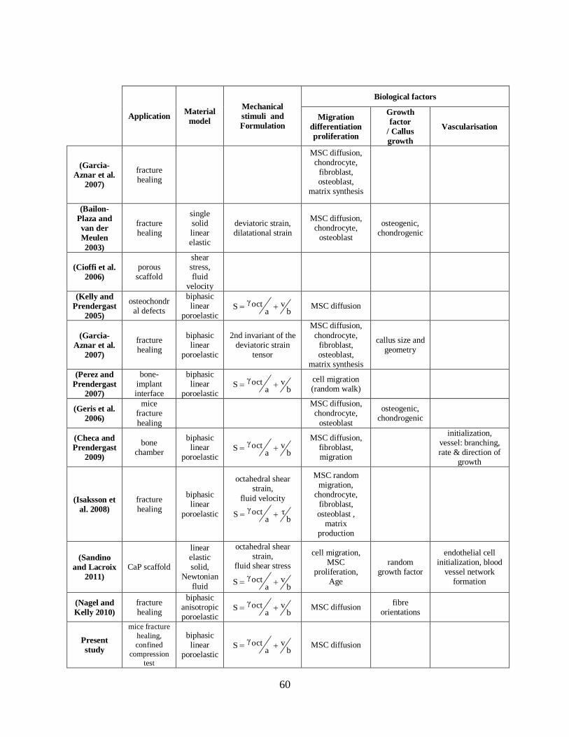
60

Application Material

model

Mechanical

stimuli and

Formulation

Biological factors

Migration

differentiation

proliferation

Growth

factor

/ Callus

growth

Vascularisation

(Garcia-

Aznar et al.

2007)

fracture healing


fibroblast, osteoblast,

matrix synthesis

(Bailon-

Plaza and

van der

Meulen

2003)

fracture healing


deviatoric strain, dilatational strain


osteoblast


(Cioffi et al.

2006)

porous scaffold

shear stress, fluid

velocity

(Kelly and

Prendergast

2005)

osteochondral defects

biphasic linear

poroelastic b

va

octγS MSC diffusion

(Garcia-

Aznar et al.

2007)

fracture healing

biphasic linear

poroelastic

2nd invariant of the deviatoric strain

tensor

MSC diffusion,

chondrocyte, fibroblast, osteoblast,

matrix synthesis

callus size and geometry

(Perez and

Prendergast

2007)

bone-implant interface

biphasic linear

poroelastic b

va

octγS

cell migration (random walk)

(Geris et al.

2006)

mice fracture

healing


osteoblast


(Checa and

Prendergast

2009)

bone chamber

biphasic linear

poroelastic b

va

octγS

MSC diffusion, fibroblast, migration

initialization, vessel: branching, rate & direction of

growth

(Isaksson et

al. 2008)

fracture healing

biphasic linear

poroelastic


fluid velocity

bη

aoctγ

S

MSC random migration,

chondrocyte, fibroblast,

osteoblast , matrix

production

(Sandino

and Lacroix

2011)

CaP scaffold

linear elastic solid,

Newtonian

fluid


fluid shear stress

bv

aoctγ

S

cell migration, MSC

proliferation, Age

random growth factor

endothelial cell initialization, blood

vessel network formation

(Nagel and

Kelly 2010)

fracture healing

biphasic anisotropic poroelastic

bv

aoctγ

S MSC diffusion fibre

orientations

Present

study

mice fracture

healing,

confined

compression

test

biphasic linear

poroelastic b

va

octγS MSC diffusion

61

Chapter Three: Development and Verification of the Finite Element Model

In this chapter, the development and validation of the finite element model are presented. Section

1 reviews bone mechanics and its behaviour under different mechanical conditions. In section 2,

a brief review of biphasic theory in orthopaedic applications is presented. Section 3 outlines the

theory and algorithms that have been developed to predict tissue distribution during fracture

repair. Next, the finite element model implemented in this study was qualitatively validated

against a previously published numerical-experimental study of Isaksson et al. (2006). Finally,

two case studies simulating experimental tissue differentiation (Bishop et al. 2006, Gardner et al.

2006) are presented as further validation of the differentiation algorithms. A summary of the

overall model development and verification is shown in Figure 3.1.

Figure 3.1. Summary of model development and verification.

3.1 Bone mechanics

The mechanical properties of bone are related to its ability to absorb shocks and resist static or

cyclic compression, tension, torsion and shearing stress loads. A comprehensive description of

the mechanical properties of bone is needed to understand the functional adaptation of the

skeletal system. Uniaxial testing (tension or compression) or three-point bending methods have

62

been used to measure mechanical properties such as bone strength and stiffness. The measured

properties can be compared in diseased versus healthy bone to diagnose musculoskeletal diseases

(e.g. osteoporosis) or estimate fracture risk. The relationship between the applied load and the

deflection of the bone can be found from the load-displacement curve (Figure 3.2). The slope of

the linear region represents the stiffness. In addition to the stiffness, the ultimate load and

displacement, and the fracture load can be determined from the load-deflection curve. The area

under the curve represents the amount of work required to rupture the bone.

Figure 3.2. The force-displacement plot representing bone behaviour (Cole et al. 2010).

The corresponding stress-strain curve can be obtained knowing the cross sectional area and the

original length. The slope of the stress-strain urve within the elasti se tion denotes Young‟s

modulus (stiffness) of the bone and the ultimate stress represents the strength. The area under the

curve represents the bone toughness. Toughness is the amount of energy that bone can withstand

before fracture takes place.

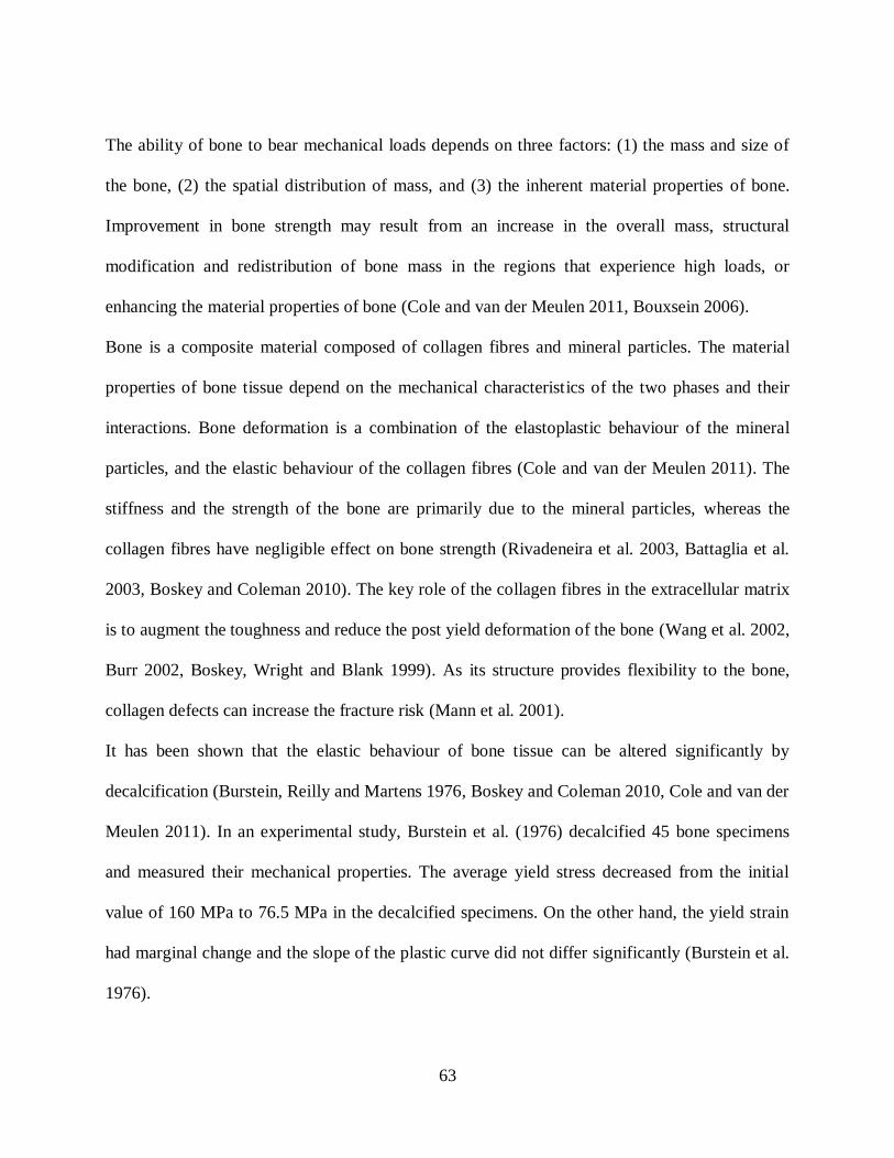
63

The ability of bone to bear mechanical loads depends on three factors: (1) the mass and size of

the bone, (2) the spatial distribution of mass, and (3) the inherent material properties of bone.

Improvement in bone strength may result from an increase in the overall mass, structural

modification and redistribution of bone mass in the regions that experience high loads, or

enhancing the material properties of bone (Cole and van der Meulen 2011, Bouxsein 2006).

Bone is a composite material composed of collagen fibres and mineral particles. The material

properties of bone tissue depend on the mechanical characteristics of the two phases and their

interactions. Bone deformation is a combination of the elastoplastic behaviour of the mineral

particles, and the elastic behaviour of the collagen fibres (Cole and van der Meulen 2011). The

stiffness and the strength of the bone are primarily due to the mineral particles, whereas the

collagen fibres have negligible effect on bone strength (Rivadeneira et al. 2003, Battaglia et al.

2003, Boskey and Coleman 2010). The key role of the collagen fibres in the extracellular matrix

is to augment the toughness and reduce the post yield deformation of the bone (Wang et al. 2002,

Burr 2002, Boskey, Wright and Blank 1999). As its structure provides flexibility to the bone,

collagen defects can increase the fracture risk (Mann et al. 2001).

It has been shown that the elastic behaviour of bone tissue can be altered significantly by

decalcification (Burstein, Reilly and Martens 1976, Boskey and Coleman 2010, Cole and van der

Meulen 2011). In an experimental study, Burstein et al. (1976) decalcified 45 bone specimens

and measured their mechanical properties. The average yield stress decreased from the initial

value of 160 MPa to 76.5 MPa in the decalcified specimens. On the other hand, the yield strain

had marginal change and the slope of the plastic curve did not differ significantly (Burstein et al.

1976).

64

Disease, injury and aging can change the mechanical behaviour of the bone. For example,

mineralization is higher and the size of mineral crystals is larger in older bones than in younger

bones. As shown in Figure 3.3, higher mineralized bones are stiffer and more brittle (lower

deflection) (Currey 2012, Jepsen and Andarawis-Puri 2012, Boskey and Coleman 2010). Hence,

less work is required to fracture bones with higher mineral contents. A bone from a child has

been shown to have larger ultimate deflection and be less stiff compared to an adult bone.

35

30

25

20

15

0

Young‟s m

odulus [M

a]

10

5

200 220 240 260 280 300

Mineral [mg ]

200 220 240 260 280 300

Mineral [mg ]

Wo

rk [

MJ

]20

10

5

2

0.2

1

0.5

(b)(a)

Figure 3.3. Relationship between the mineral content and bone mechanical properties: (a)

by increasing the mineral density, the stiffness increases, (b) while an increase in the bone

mineral content leads to more brittleness (Currey 2012).

During growth, bone mass increases in the first 30 years, then there is no significant change in

the bone mass for approximately 10 years. Around age 40, there is a gradual loss in bone mass.

Bone loss initiates earlier in life for women and increases at a higher rate, especially after

menopause than for males. Due to the accelerated bone loss in women, the risk of fracture is

higher: 40 % for women and 13-25 % for men (Figure 3.4) (McDonnell et al. 2007). Moreover,

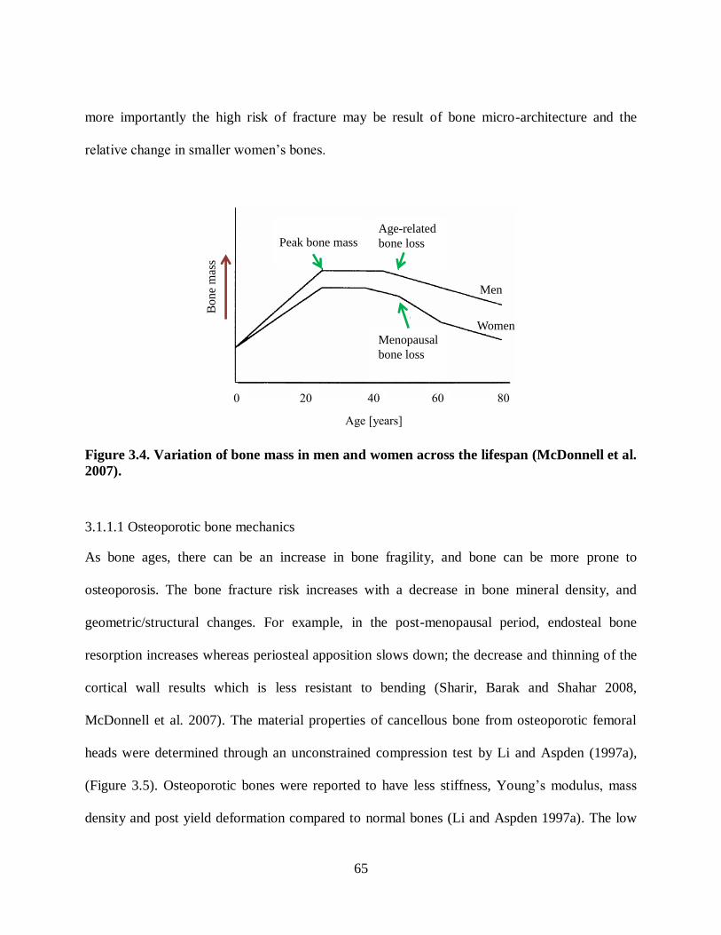
65

more importantly the high risk of fracture may be result of bone micro-architecture and the

relative hange in smaller women‟s ones.

Peak bone massAge-related

bone loss

Menopausal

bone loss

Women

Men

0 20 40 60 80

Bone

mas

s

Age [years]

Figure 3.4. Variation of bone mass in men and women across the lifespan (McDonnell et al.

2007).

3.1.1.1 Osteoporotic bone mechanics

As bone ages, there can be an increase in bone fragility, and bone can be more prone to

osteoporosis. The bone fracture risk increases with a decrease in bone mineral density, and

geometric/structural changes. For example, in the post-menopausal period, endosteal bone

resorption increases whereas periosteal apposition slows down; the decrease and thinning of the

cortical wall results which is less resistant to bending (Sharir, Barak and Shahar 2008,

McDonnell et al. 2007). The material properties of cancellous bone from osteoporotic femoral

heads were determined through an unconstrained compression test by Li and Aspden (1997a),

(Figure 3.5). Osteoporotic bones were reported to have less stiffness, Young‟s modulus, mass

density and post yield deformation compared to normal bones (Li and Aspden 1997a). The low

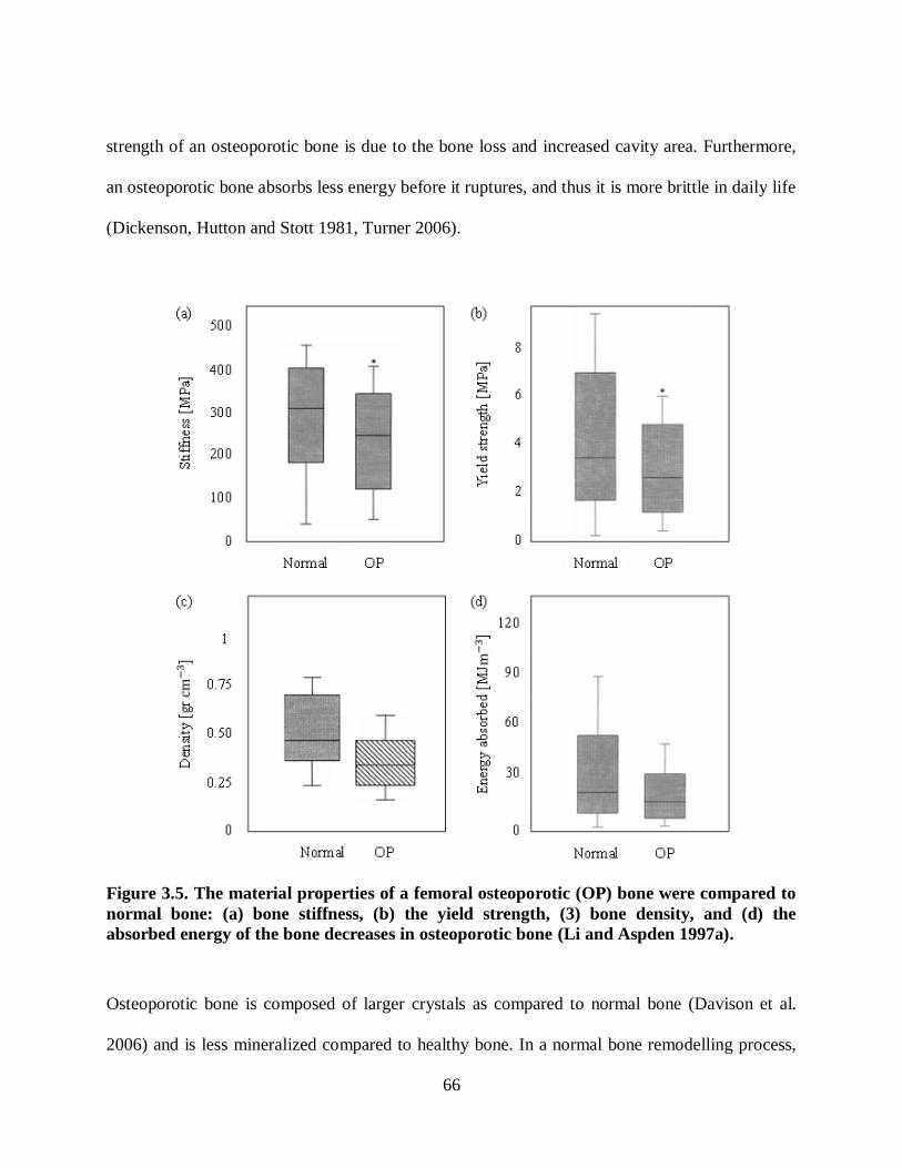
66

strength of an osteoporotic bone is due to the bone loss and increased cavity area. Furthermore,

an osteoporotic bone absorbs less energy before it ruptures, and thus it is more brittle in daily life

(Dickenson, Hutton and Stott 1981, Turner 2006).

Figure 3.5. The material properties of a femoral osteoporotic (OP) bone were compared to

normal bone: (a) bone stiffness, (b) the yield strength, (3) bone density, and (d) the

absorbed energy of the bone decreases in osteoporotic bone (Li and Aspden 1997a).

Osteoporotic bone is composed of larger crystals as compared to normal bone (Davison et al.

2006) and is less mineralized compared to healthy bone. In a normal bone remodelling process,

67

the osteoclasts resorb bone and the cavity is immediately filled with a collagenous osteoid.

Primary mineralization usually begins after a few days and continues until the remodelling cavity

has been 50 to 60 % filled. Next, the secondary mineralization begins at a slower pace and the

cavity will be filled to the maximum level of 90 to 95 % over years. In an osteoporotic bone,

with the increased levels of bone resorption, there is less time for secondary mineralization,

resulting in a lower stiffness (Roschger et al. 2001). Tingart et al. (2003) found that the mineral

density in a 87-year-old man is 0.17 2cm

gr in humeral head and is 0.23

2cm

gr at the surgical neck,

whereas these numbers are 0.5 and 0.55 2cm

gr for a 65-year-old man, respectively (Figure 3.6).

Humeral

head

Surgical

neck

(b)(a)

Figure 3.6. The radiographs of the proximal humerus in (a) a 87-year-old man with low

bone mineral density and, (b) a 65-year-old man with higher mineral density (Tingart et al.

2003).

In osteoporotic patients, the vertical trabeculae are the ones left standing and bear the greater

loads, compared to the horizontal trabeculae that have been absorbed to a greater extent. This

makes the trabecular structure anisotropic and weaker in the horizontal direction (Thomsen,

Ebbesen and Mosekilde 2002). In a computational study, the strain in the head of an osteoporotic

68

femur was 70 % higher and less uniformly distributed compared to the no osteoporotic femur

(Van Rietbergen et al. 2003). The bone porosity increases with age (Figure 3.7) leading to bone

loss and lower bone strength. McCalden et al. (1993) reported that bone porosity is higher for

women compared with men after age 70. The relationship etween the density and the Young‟s

modulus of the subchondral bone plate from the femoral head has been determined in

osteoporotic and normal bones (Figure 3.8) (Li and Aspden 1997b).

30

20

10

020 40 60 80 100 1200

Poro

sity

[%

]

Age [years]

female

0.29827x5.6662y

male

0.13010x2.1774y

male

female

Figure 3.7. The graph demonstrates the relationship between porosity and age for men and

women (McCalden et al. 1993).

0 20 40 60 80 60 80

5

10

15

20

25

normal

10.516.6ρE

icosteoporot

21.422.1ρE

Sti

ffn

ess

[GP

a]

Density [gr ]

Figure 3.8. The relationship between stiffness and density of the subchondral bone plate (Li

and Aspden 1997b).

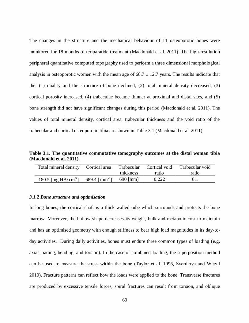
69

The changes in the structure and the mechanical behaviour of 11 osteoporotic bones were

monitored for 18 months of teriparatide treatment (Macdonald et al. 2011). The high-resolution

peripheral quantitative computed topography used to perform a three dimensional morphological

analysis in osteoporotic women with the mean age of 68.7 ± 12.7 years. The results indicate that

the: (1) quality and the structure of bone declined, (2) total mineral density decreased, (3)

cortical porosity increased, (4) trabeculae became thinner at proximal and distal sites, and (5)

bone strength did not have significant changes during this period (Macdonald et al. 2011). The

values of total mineral density, cortical area, trabecular thickness and the void ratio of the

trabecular and cortical osteoporotic tibia are shown in Table 3.1 (Macdonald et al. 2011).

Table 3.1. The quantitative commutative tomography outcomes at the distal woman tibia

(Macdonald et al. 2011).

Total mineral density Cortical area Trabecular

thickness

Cortical void

ratio

Trabecular void

ratio

180.5 [mg HA/ 3cm ] 689.4 [2mm ] 690 [mm] 0.222 8.1

3.1.2 Bone structure and optimisation

In long bones, the cortical shaft is a thick-walled tube which surrounds and protects the bone

marrow. Moreover, the hollow shape decreases its weight, bulk and metabolic cost to maintain

and has an optimised geometry with enough stiffness to bear high load magnitudes in its day-to-

day activities. During daily activities, bones must endure three common types of loading (e.g.

axial loading, bending, and torsion). In the case of combined loading, the superposition method

can be used to measure the stress within the bone (Taylor et al. 1996, Sverdlova and Witzel

2010). Fracture patterns can reflect how the loads were applied to the bone. Transverse fractures

are produced by excessive tensile forces, spiral fractures can result from torsion, and oblique

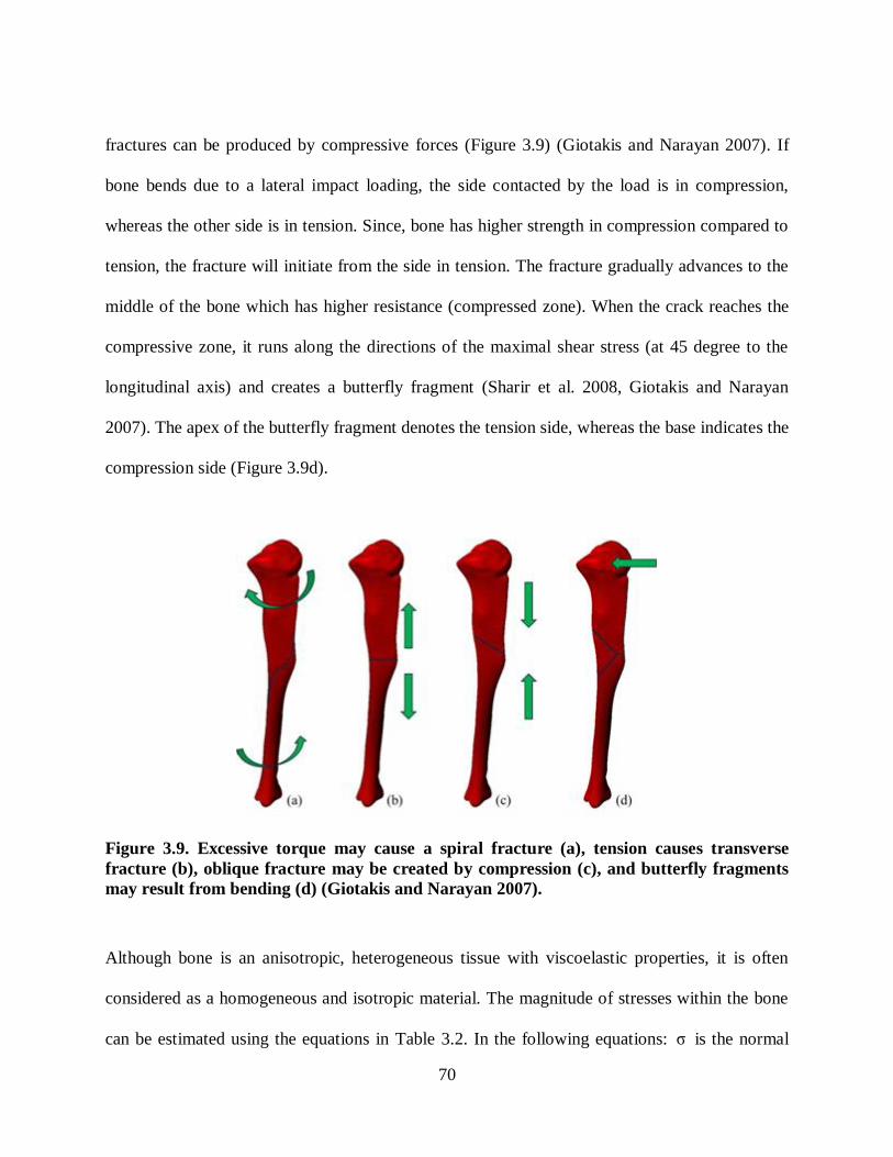
70

fractures can be produced by compressive forces (Figure 3.9) (Giotakis and Narayan 2007). If

bone bends due to a lateral impact loading, the side contacted by the load is in compression,

whereas the other side is in tension. Since, bone has higher strength in compression compared to

tension, the fracture will initiate from the side in tension. The fracture gradually advances to the

middle of the bone which has higher resistance (compressed zone). When the crack reaches the

compressive zone, it runs along the directions of the maximal shear stress (at 45 degree to the

longitudinal axis) and creates a butterfly fragment (Sharir et al. 2008, Giotakis and Narayan

2007). The apex of the butterfly fragment denotes the tension side, whereas the base indicates the

compression side (Figure 3.9d).

Figure 3.9. Excessive torque may cause a spiral fracture (a), tension causes transverse

fracture (b), oblique fracture may be created by compression (c), and butterfly fragments

may result from bending (d) (Giotakis and Narayan 2007).

Although bone is an anisotropic, heterogeneous tissue with viscoelastic properties, it is often

considered as a homogeneous and isotropic material. The magnitude of stresses within the bone

can be estimated using the equations in Table 3.2. In the following equations: ζ is the normal

71

stress, η is the shear stress, M is the bending moment, T is the applied torsion, xxI is the areal

moment of inertia about x-axis, J is the polar moment of inertia about the torsional axis, pr and

er are the periosteal (outer) radius and endosteal (inner) radius of the bone. The geometry of

cortical bone alters with age: the periosteal radius increases as a result of periosteum apposition,

whereas the endosteal radius decreases due to bone resorption. The outer diameter of the cortical

section gets larger and the total thickness becomes thinner (less cross sectional area).

Using the simplified bending equation in Table 3.2, three cases were compared: (1) a reference

bone with a solid circular cross section, (2) a young bone, and (3) an adult bone (Figure 3.10).

The material properties of the young bone, with hollow cross section and same periosteal

diameter as the reference bone were compared with the reference bone. Although the young bone

had 25 % less bone mass, it was only 6 % weaker than the reference bone. On the other hand, an

increase of 76 % was observed in the bending stiffness of an adult bone that had a larger outer

diameter (a 25 % increase) but same bone mass as the reference bone due to mass redistribution

(Figure 3.10, Cole and van der Meulen 2011). The bone mass was distributed further from the

bending plane compared to the young bone. Since the moment of inertia ( xxI ) is proportional to

the difference of the radius to the 4th power (

4

e

4

p rr ), the stiffness increased from 94% to 170%.

Table 3.2. Estimation of normal stress under axial, bending and torsional loads.

Cross sectional area Areal moment of inertia Axial Bending Torsion

2

e

2

p rrπA

xx

4

e

4

pxx

2IJ

rrπ4

1I

A

Fζ

xx

px

maxI

rMζ

J

Trp

max

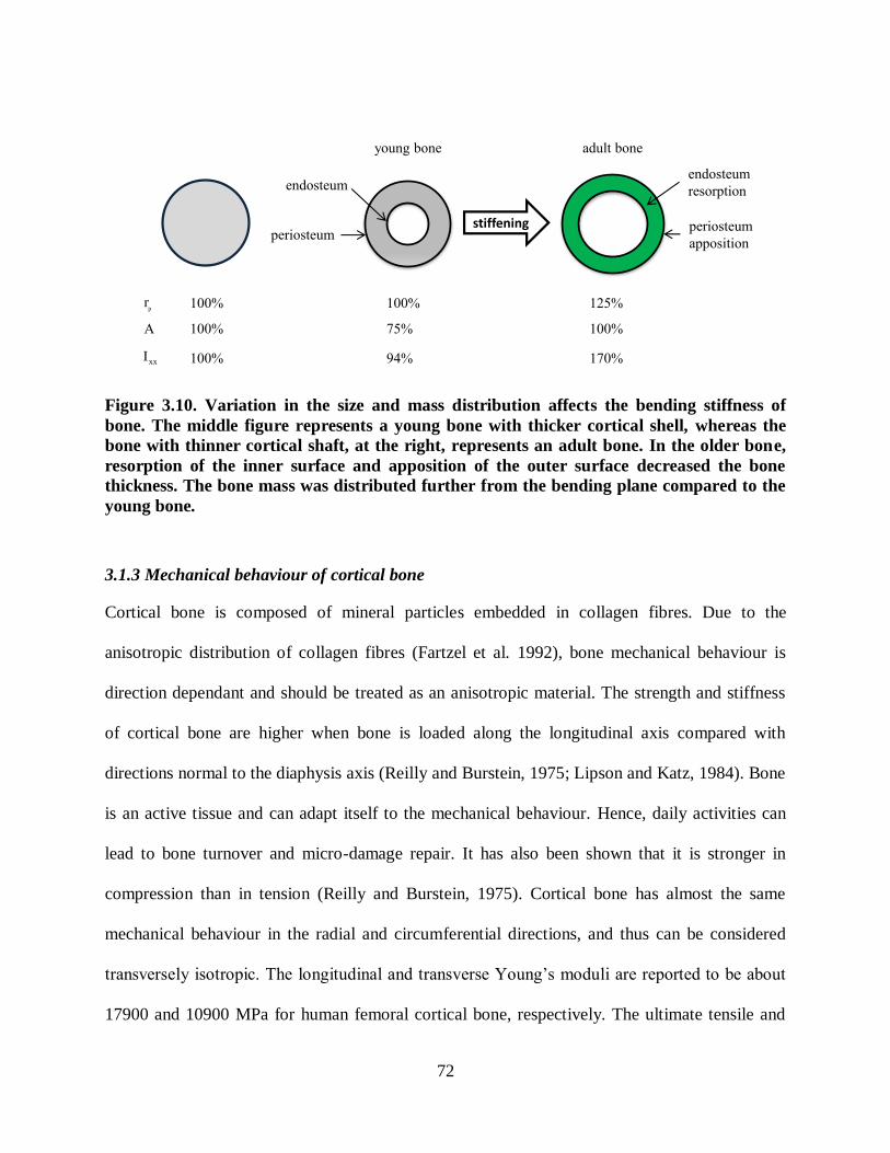
72

periosteumperiosteum

apposition

endosteum

resorptionendosteum

stiffening

young bone adult bone

100% 100% 125%

A 100% 75% 100%

100% 94% 170%xxI

pr

Figure 3.10. Variation in the size and mass distribution affects the bending stiffness of

bone. The middle figure represents a young bone with thicker cortical shell, whereas the

bone with thinner cortical shaft, at the right, represents an adult bone. In the older bone,

resorption of the inner surface and apposition of the outer surface decreased the bone

thickness. The bone mass was distributed further from the bending plane compared to the

young bone.

3.1.3 Mechanical behaviour of cortical bone

Cortical bone is composed of mineral particles embedded in collagen fibres. Due to the

anisotropic distribution of collagen fibres (Fartzel et al. 1992), bone mechanical behaviour is

direction dependant and should be treated as an anisotropic material. The strength and stiffness

of cortical bone are higher when bone is loaded along the longitudinal axis compared with

directions normal to the diaphysis axis (Reilly and Burstein, 1975; Lipson and Katz, 1984). Bone

is an active tissue and can adapt itself to the mechanical behaviour. Hence, daily activities can

lead to bone turnover and micro-damage repair. It has also been shown that it is stronger in

compression than in tension (Reilly and Burstein, 1975). Cortical bone has almost the same

mechanical behaviour in the radial and circumferential directions, and thus can be considered

transversely isotropi . The longitudinal and transverse Young‟s moduli are reported to e a out

17900 and 10900 MPa for human femoral cortical bone, respectively. The ultimate tensile and

73

compressive stresses in the longitudinal direction are about 135 and 205 MPa, whereas for the

transverse direction these values are about 53 and 131 MPa, respectively. The ultimate shear

stress is reported to be 65 MPa. These values demonstrate the relatively low strength of cortical

bone in shear, and the stiffer behaviour in the longitudinal direction (Reilly and Burstein, 1975).

Cortical bone is quite brittle and cannot bear large strains beyond the yield point. The stress-

strain behaviour of human cortical bone is presented in Figure 3.11.

Figure 3.11. The stress-strain curve illustrates that bone is stiffer in the longitudinal

i c ion. Yo ng’s mo l s is h s m in nsion n comp ssion, whereas in

compression bone has more strength (Kutz 2003).

The creep response of cortical bone has been evaluated under low, intermediate and high stress

levels. In low and moderate loading levels, bone returns to its original state, whereas at higher

stress levels, close to the yield point, permanent residual strain will develop (Fondrk, 1988).

Several factors can affect the mechanical behaviour of the cortical bone such as porosity,

mineralization and aging. A marginal increase in the bone mineralization may lead to a higher

Young‟s modulus and strength (Boskey and Coleman 2010, Cole and van der Meulen 2011). In

74

contrast, aging of bone tissue can have a negative effect on the tissue strength. The ultimate

tensile stress and Young‟s modulus of ti ial orti al one were determined in ompression tests

across the lifespan (Burstein et al. 1976). The results indicate a 2 % and 4.7 % decrease per

decade for the ultimate stress and modulus, respectively (Figure 3.12).

Figure 3.12. Yo ng’s mo l s n l im stress of tibial cortical bone decrease with

increasing age. The rate of decrease is higher for ultimate stress compared to the modulus

(Burstein et al. 1976).

Cortical bone is a viscoelastic material exhibiting both viscous and elastic properties. The

loading rate moderately affects the mechanical behaviour of the tissue. The strain rate sensitivity

has been evaluated in a uniaxial tension test. The stress-strain curves were obtained while strain

rate was increasing by six orders of magnitude from 0.001 to 1500 % per second. Daily activities

occur in a range of strain rates between 0.01 to 1.0 % per second and the higher strain rates can

be the result of car accidents or gunshots. The results indicate that Young`s modulus and ultimate

stress change by a factor of 2 and 3, respectively. As shown in Figure 3.13, the strain rate in the

range of daily activities has only a minor effect on the stiffness of the tissue (Kutz 2003).

75

Figure 3.13. The response of cortical bone under different strain rates (Kutz 2003).

3.1.4 Mechanical behaviour of cancellous bone

Trabecular bone is a heterogeneous material, i.e., its material properties vary spatially. In

addition to the inhomogeneity, cancellous bone is anisotropic (i.e. the physical behaviour of the

tissue differs in each direction).

At the end of long bones, cancellous struts and plates transfer large forces to the strong midshaft.

The irregular shape and small size of the struts make the measurement of trabecular bone

diffi ult. The reported Young‟s modulus for tra e ular one ranges from 1 to 19 GPa (Ashman

and Rho 1988, Rho, Hobatho and Ashman 1995). According to Neibur et al. (2000), trabecular

bone ultimate stress is higher in compression than in tension. Both stiffness and strength of the

tissue decrease 10 % per decade (Mosekilde and Danielsen 1987, Lakes and Saha 1979). When

trabecular bone is compressed greater than the ultimate load, the stiffness will be reduced and if

reloaded will develop higher strains (Figure 3.14).

76

Figure 3.14. The stress-strain plot for a load-unload-reload trabecular sample. The loading

s s poin 1, i is nlo poin 2 n lo poin 3. Th ini i l Yo ng’s

modulus from the linear section of the reloading (3-4) is the same as the original Young’s

modulus (1-2) at the beginning, but reduces quickly to residualE . A permanent residual strain

residualε will be developed (Keaveny, Wachtel and Kopperdahl 1999).

Keaveny et al. (1999) concluded that excessive loads cause residual strain and geometric

changes which increase the risk of fracture by significantly decreasing the mechanical

properties of the underlying trabecular bone (Figure 3.14).

3.2 Soft tissue biphasic theory

Soft tissues such as fibrous tendons and ligaments, cartilage, bone and granulation matrix are

composed of a solid matrix and significant amounts of interstitial fluid (van der Meulen and

Huiskes 2002, Van der Voet 1992). To determine the mechanical response of the tissues, the

behaviour of each phase should be considered as well as the interactions between the phases (the

solid displacements and fluid velocities).

The fluid related time dependent structural analysis of soft tissues can be described in two ways:

(1) poroelastic theory, or (2) mixture theory. In the poroelastic theory, material is considered as a

porous solid which is fully saturated with fluid. This theory has been developed to describe the

77

behaviour of soil (Biot, 1941). The biphasic theory considers the material as a more general

continuum mixture of solid and fluid phases. Mow et al. (1980) employed iot‟s (1941)

biphasic theory to describe the two-phase behaviour of soft tissues, used by Ateshian et al.

(1994) to determine the importance of interstitial fluid in the load support mechanism of articular

cartilage (Mow et al. 1980, Ateshian et al. 1994). It has been proven that the poroelastic theory is

equivalent to the biphasic theory when the fluid phase is considered inviscid (Mow et al. 1980,

Simon 1992). Due to the complex structure of soft tissues, complexity of the applied loads and

material properties, and thus limited availability of analytical solutions, the use of numerical

methods and finite element models (FEM) is essential. It has been shown that FEM packages,

e.g. ABAQUS, can be used to analyse the biphasic behaviour of soft tissues with reasonable

accuracy (Prendergast, van Driel and Kuiper 1996, Van der Voet 1992, Wu, Herzog and Epstein

1998). In the following section, the biphasic theory for soft tissues is briefly summarized

(Ateshian et al. 1994, Mow et al. 1980).

The behaviour of tissues in a free draining confined compression test can be explained by the

movement of the interstitial fluid. As shown in Figure 3.15, a ramp displacement was applied to

the articular cartilage (OAB) and kept constant for the rest of the test (BCDE). Immediately after

application of an axial compression load, the stress increases due to the pressurization of the

fluid phase. The fluid is forced out of the tissue as the load increases, and continues to flow even

when the displacement is kept constant. The redistribution of the fluid leads to stress relaxation

and a steady state condition is reached. The stress at the equilibrium state represents the stress

within the solid phase (Mow et al. 1980).

78

Figure 3.15. (a) Movement of fluid when tissue is under a free draining confined

compression test, (b) ramp deformation is applied (increased with a linear ramp to B and

remained constant from B to E, (b) the flow exudes immediately after the deformation is

applied and the stress reaches its maximum amount (B). The fluid continues to flow. The

tissue reaches an equilibrium point and the stress decreases and reaches a plateau (E)

(Mow et al. 1980).

3.2.1 Kinematics

Bone tissue can be modelled as a two-phase material: a porous, linear elastic,

isotropic/anisotropic, homogeneous solid matrix with constant isotropic permeability and an

incompressible, inviscid fluid phase. To define quantities associated with solid and fluid phases,

the superscripts s and f are used, respectively. The tissue volume element (dV) consists of a

sufficient number of solid grains sdV , and volume of interstitial fluid fdV . The medium is

assumed to be fully saturated and the voids completely filled with the fluid. Hence, we get:

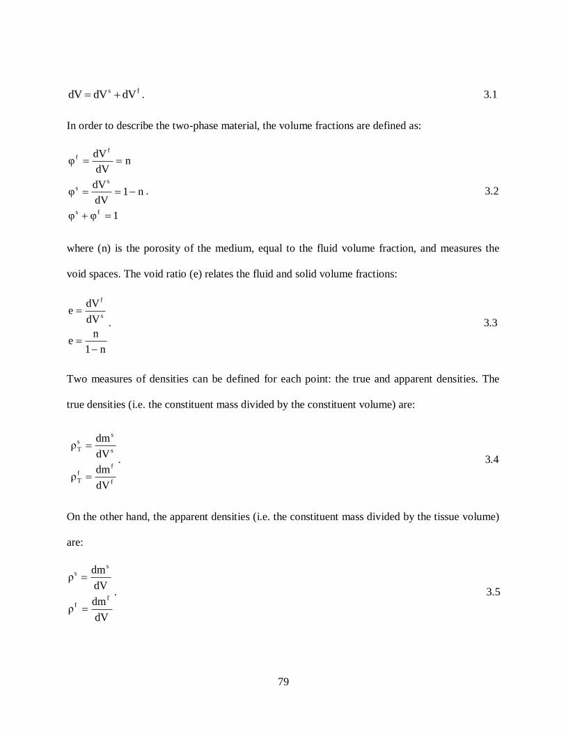
79

fs dVdVdV . 3.1

In order to describe the two-phase material, the volume fractions are defined as:

1θθ

n1dV

dVθ

ndV

dVθ

fs

ss

ff

. 3.2

where (n) is the porosity of the medium, equal to the fluid volume fraction, and measures the

void spaces. The void ratio (e) relates the fluid and solid volume fractions:

n1

ne

dV

dVe

s

f

. 3.3

Two measures of densities can be defined for each point: the true and apparent densities. The

true densities (i.e. the constituent mass divided by the constituent volume) are:

f

ff

T

s

ss

T

dV

dmρ

dV

dmρ

. 3.4

On the other hand, the apparent densities (i.e. the constituent mass divided by the tissue volume)

are:

dV

dmρ

dV

dmρ

ff

ss

. 3.5

80

The total apparent density ( ) of the mixture is the sum of solid sρ and fluid fρ apparent

densities, which can be expressed as follows:

fs nρρn1ρ . 3.6

According to the continuum mixture theory, each component has its own motion. Every spatial

position x in the mixture is simultaneously filled by the material solid sX and fluid f

X

constituents at any time t. The fluid particles and solid grains in the solid skeleton are moving

with different velocities in different directions and at different positions. However, these details

are ignored and an average motion for each material point is considered (Truesdell 1966). The

motion of the solid and fluid constituents can be described by a mapping between reference

and current configurations, where s

iX and f

iX are arbitrary material points in the reference

configuration, and s

ix and f

ix in the current configuration:

t,Xx

t,Xx

f

i

f

i

f

i

s

i

s

i

s

i

. 3.7

The average displacement vector can be defined for solid and fluid phases separately as follows:

f

i

f

i

f

i

f

i

s

i

s

i

s

i

s

i

Xt,Xu

Xt,Xu

. 3.8

Then the relative fluid displacement is then given by (Biot, 1941):

s

i

f

i

f

i uuθw . 3.9

where s

iu and f

iu are the primary unknown fields.

3.2.2 Conservation of mass

The balance of mass for the solid and fluid particles can be expressed as:

81

0vtρdiv

t

tρ sss

. 3.10

0vtρdiv

t

tρ fff

. 3.11

where div is the divergence operator.

The solid and fluid constituents are assumed to be intrinsically incompressible. Hence, the

continuity equation for the whole mixture can be obtained by adding equations 3.10 and 3.11 to

give:

0vvdiv ffss . 3.12

3.2.3 Conservation of linear momentum

For the biphasic theory, the solid sσ and fluid f

σ stress tensors can be expressed as follows:

v

ijij

ff

ij

e

ijij

ss

ij

ζpδθζ

ζpδθζ

. 3.13

where e

σ is the elastic stress of the solid, v

σ is the viscous stress of the fluid, and p is the fluid

pore pressure. The elastic effective stress is taken to be positive in tension, whereas pore pressure

in the fluid is assumed to be positive in compression. The fluid is considered inviscid in our

study. Therefore, the viscous shear stress is considered null within the fluid 0vσ . This is an

acceptable assumption because when a fluid flows through a porous material a viscous drag force

much greater than the fluid shear stress is applied to the solid skeleton.

According to the principle of effective stress, the total stress σ of the mixture can be

decomposed in two parts: (1) the pore pressure (p) in the fluid acting on the solid skeleton and in

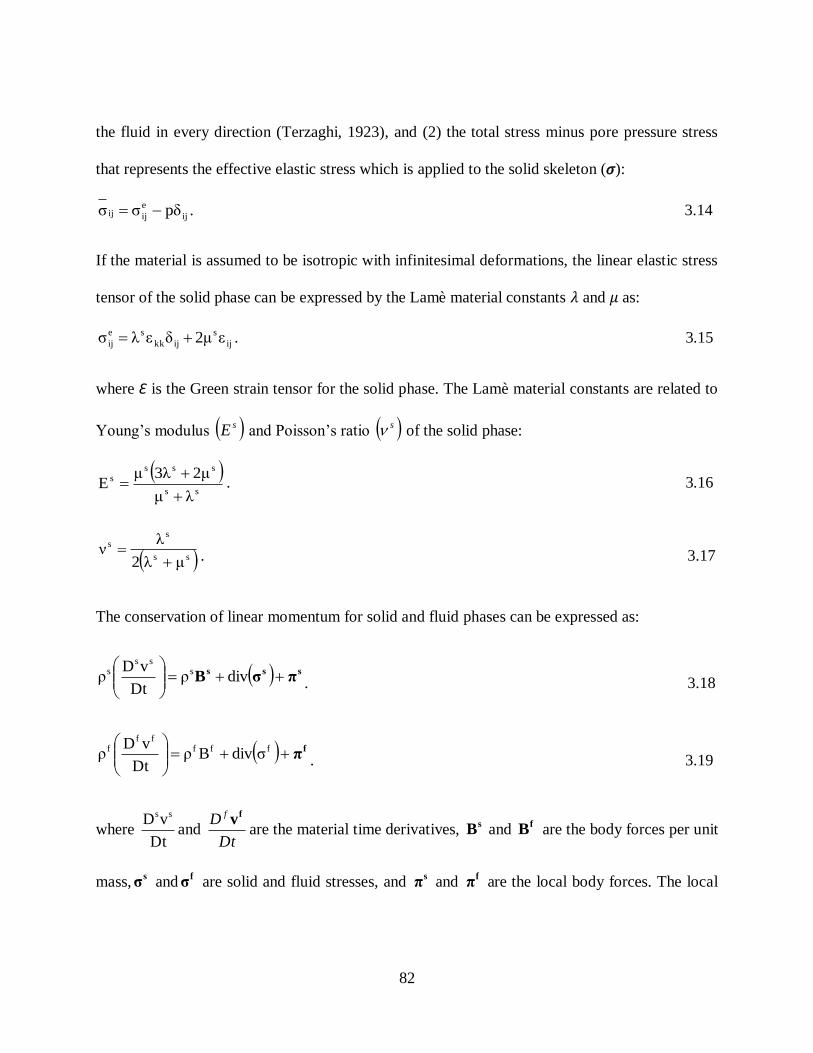
82

the fluid in every direction (Terzaghi, 1923), and (2) the total stress minus pore pressure stress

that represents the effective elastic stress which is applied to the solid skeleton ( ):

ij

e

ijij pδζζ . 3.14

If the material is assumed to be isotropic with infinitesimal deformations, the linear elastic stress

tensor of the solid phase can be expressed by the Lamè material constants and as:

ij

s

ijkk

se

ij ε2μδελζ . 3.15

where Ɛ is the Green strain tensor for the solid phase. The Lamè material constants are related to

Young‟s modulus sE and oisson‟s ratio s of the solid phase:

ss

ssss

λμ

2μ3λμE

. 3.16

ss

ss

μλ2

λν

. 3.17

The conservation of linear momentum for solid and fluid phases can be expressed as:

sssπσB

divρ

Dt

vDρ s

sss

. 3.18

fπ

fffff

f ζdivBρDt

vDρ . 3.19

where Dt

vD ss

and Dt

D f fv

are the material time derivatives, s

B and f

B are the body forces per unit

mass,s

σ andf

σ are solid and fluid stresses, and s

π and f

π are the local body forces. The local

83

body forces account for the interactions between the solid and fluid constituents that must

satisfy:

s

i

f

i

s

i

f

i vvKvvK

fsππ

. 3.20

where K is the diffusive drag coefficient and is related to the permeability (k) of the tissue, which

is considered constant in our study (Ysart and Mason 1994, Lai, Mow and Roth 1981):

k

θK

2f

. 3.21

Assuming the external body forces and the fluid and solid accelerations are negligible, the

momentum equation for the constituents and the medium is given by:

0πσ

0πσss

ffdiv

div. 3.22

0σσσfs divdiv . 3.23

Substituting the obtained solid and fluid stress equations into the solid and fluid momentum

equations leads to:

pk

t

div

divgradμλpgrad

2

2ss

s

ss

u

0uus

. 3.24

The FE solver ABAQUS v6.11 was used in the current study, in which a porous medium is

modelled as a multiphase material: solid particles and one or more fluids. The fluid phase is

composed of a liquid phase and the other is often gas. The wetting liquid is assumed to be

relatively incompressible, whereas gas is relatively compressible. When the porous medium is

84

considered fully saturated, the voids are completely filled with the wetting liquid (e.g. in the

present study). The elementary volume (dV) is the sum of the grains of solid phase gdV and the

volume of fluid phase fdV . ABAQUS calculates the effective stress, *

σ , as follows:

Iσσ*

auX1Xuw . 3.25

where σ is the total stress, wu and au are pressure stresses in the wetting liquid and the other

fluid, respectively. When the medium is fully saturated, X is equal to 1.0.

The porous medium is modelled by attaching the finite element mesh to the solid phase and the

wetting liquid can flow through this mesh. The mechanical part of the model is based on the

effective stress principal. For the fluid phase, the rate of increase in the fluid mass at a point

should be equal to the rate of mass of fluid flowing to that point (i.e. continuity equation). The

fluid flow is defined y the Dar y‟s law. The mass ontinuity equation is relative to the fluid

pore pressure. A negative pore pressure represents a suction condition. In a transient analysis, a

backward difference operator is used to integrate the continuity equation; the accuracy of the

analysis is controlled by the selected time integration and the maximum pore pressure.

The Young‟s modulus and oisson ratio are defined in A AQUS and then the Lamè material

constants of the solid phase calculated to find the stress in the solid grains. The void ratio (e) and

permeability are also defined in ABAQUS. Since ABAQUS uses the poroelasticity theory, the

introduced permeability in the biphasic model (k) (Mow et al. 1980) needs to be converted to the

poroelastic permeability ( k ):

γkk . 3.26

where

3mm

N0681.9 e is the specific weight of the interstitial fluid (Wu et al. 1998).

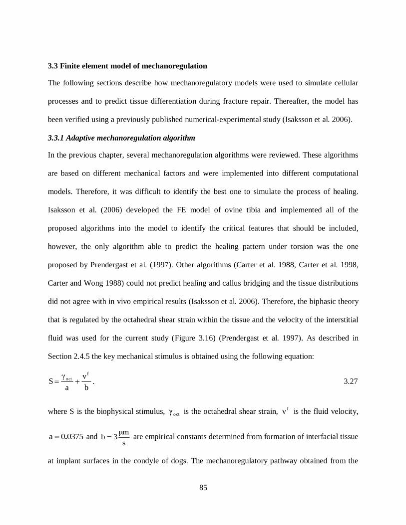
85

3.3 Finite element model of mechanoregulation

The following sections describe how mechanoregulatory models were used to simulate cellular

processes and to predict tissue differentiation during fracture repair. Thereafter, the model has

been verified using a previously published numerical-experimental study (Isaksson et al. 2006).

3.3.1 Adaptive mechanoregulation algorithm

In the previous chapter, several mechanoregulation algorithms were reviewed. These algorithms

are based on different mechanical factors and were implemented into different computational

models. Therefore, it was difficult to identify the best one to simulate the process of healing.

Isaksson et al. (2006) developed the FE model of ovine tibia and implemented all of the

proposed algorithms into the model to identify the critical features that should be included,

however, the only algorithm able to predict the healing pattern under torsion was the one

proposed by Prendergast et al. (1997). Other algorithms (Carter et al. 1988, Carter et al. 1998,

Carter and Wong 1988) could not predict healing and callus bridging and the tissue distributions

did not agree with in vivo empirical results (Isaksson et al. 2006). Therefore, the biphasic theory

that is regulated by the octahedral shear strain within the tissue and the velocity of the interstitial

fluid was used for the current study (Figure 3.16) (Prendergast et al. 1997). As described in

Section 2.4.5 the key mechanical stimulus is obtained using the following equation:

b

v

a

γS

foct . 3.27

where S is the biophysical stimulus, octγ is the octahedral shear strain, fv is the fluid velocity,

03750a . and s

μm3b are empirical constants determined from formation of interfacial tissue

at implant surfaces in the condyle of dogs. The mechanoregulatory pathway obtained from the

86

variation of biophysical stimuli within the interfacial tissue during the healing period

(Prendergast et al. 1997). The cell deformation of the solid and fluid phase was investigated by

calculating the octahedral shear strain and fluid flow, which were calculated from a poroelastic

analysis using ABAQUS.

The bone tissues (e.g. cortical bone and bone marrow) and the fracture site were defined as

biphasic materials. At the beginning of the analysis, the fracture site (i.e. callus) was assumed to

e filled with stem ell seeded granulation tissue. The Young‟s modulus, oisson‟s ratio,

permeability and void ratio were used to define the poroelastic properties of the tissues as listed

in Table 3.3. The continuum elements with pore pressure properties were used to mesh the

fracture models (e.g. CAX8P, C3D8P). The boundary conditions and mechanical loads were

applied to the FE model. The poroelastic analysis was conducted and the fluid velocity and

octahedral shear strain were computed at each integration point throughout the fracture site.

According to the predicted mechanical stimuli and based on the algorithm proposed by

Prendergast, the distribution of the differentiated tissue was determined (Lacroix et al. 2002,

Prendergast et al. 1997). High values for S promote the differentiation of mesenchymal stem

cells into fibrous tissues 6S3 , intermediate values stimulate cartilage differentiation

3S1 , and low levels lead to formation of immature 1S0.267 and mature bony tissue

2670S0110 .. (Figure 3.16). The material properties of the intact zone were kept constant

during the analysis.

87

Figure 3.16. Proposed biphasic algorithm by Prendergast et al. (1997); strain and fluid

velocity are the biophysical stimuli.

As bone heals, new tissues with new material properties differentiate at the fracture site. Hence,

in the computational analysis, the gradual change of material properties simulates the tissue

regeneration and the bone repair process. Changing the material properties temporally could be

achieved using an iterative process. Firstly, the poroelastic analysis calculated the mechanical

stimuli based on the bone geometry, applied loads, defined boundary conditions and material

properties (i.e. the unfractured bone, and the fracture site initially composed of granulation

tissue). Secondly, the differentiated tissues were predicted by the algorithm and the properties

were updated (Lacroix et al. 2002, Prendergast et al. 1997). Thirdly, the analysis was continued

until the mechanical stimuli reached a steady state and no further differentiation occured (i.e.

bone healed). The differentiated tissues at the fracture site were also modelled as linear

poroelastic materials. Table 3.3 illustrates the tissue material properties used (Isaksson et al.

2006). The required stages to model the iterative process are summarized in Figure 3.17.

88

Table 3.3. Poroelastic tissue material properties (Isaksson et al. 2006).

Constant (intact site) Variable (fracture site)

cortical

bone marrow granulation

tissue

fibrous

tissue cartilage

immature

bone

mature

trabecular

bone ovine tibia

E [MPa] 15750 2 0.2 2 10 1000 6000

0.325 0.167 0.167 0.167 0.167 0.325 0.325

k

Ns

mm 4

510 0.010 0.010 0.010 0.005 0.100 0.370

e 0.041 4.00 4.00 4.00 4.00 4.00 4.00

Fracture zone is initially filled with

granulation tissue. (step=1)

FE poroelastic analysis

(ABAQUS)

Fluid velocity & octahedral shear strain

in each element

Prediction of tissue phenotype using

the biphasic algorithm

Updating the material properties

Δstepstepstep

Figure 3.17. The iterative model used to simulate fracture repair.

3.3.1.1 User defined subroutine: USDFLD

During the bone healing progression, the material properties of the fractured zone change over

time. This temporal change is a function of the fluid velocity and octahedral shear strain

(Prendergast et al. 1997). A user defined subroutine (USDFLD) was written in FORTRAN, to

89

link the mechanical properties to the field variables (i.e. fluid velocity and octahedral shear

strain). The mechanical stimulus, S, was calculated at each integration point based on the

predicted fluid velocity and strain from the previous step. Therefore, by treating the mechanical

stimulus as the field variable to be computed in USDFLD, the material properties were updated

based on the fluid velocity and strain. USDFLD updated the solution-dependant material

properties of the fra ture zone (e.g. Young‟s modulus, oisson‟s ratio and permea ility) and

imported them into ABAQUS.

The USER DEFINED FIELD comment was used in ABAQUS input file to indicate the

USDFLD subroutine should be called during the analysis. One field variable, with the values

changing from 1 to 5, was chosen to define the tissue type (Figure 3.18). Table 3.4 shows how

the field variable (FV) was defined in the USDFLD. In the table, S is the mechanical stimulus, E

is the Young‟s modulus, ν is the oisson‟s ratio, k is the permea ility.

The field variable was set to be a function of the magnitude of fluid velocity (FLVEL) and

octahedral shear strain. To access the material point data the utility routine GETVRM was used,

and the values of fluid velocity and strain were stored during the analysis. The values defined in

the subroutine were not automatically stored by ABAQUS. In order to have access to the

calculated values, they must have been saved as solution dependant variables (SDV). The value

for fluid velocity was stored as SDV(1), the value of octahedral shear strain was stored as

SDV(2) and the mechanical stimulus, S, was saved as SDV(3). The stored SDVs were then used

in the following step to predict the updated material properties.

The magnitude of fluid velocity and octahedral shear strain were computed within the subroutine

using the following equations:

90

2

3

2

2

2

1 FLVELFLVELFLVELFLVEL , 3.28

2

23

2

31

2

21 EEPEEPEEPEEPEEPEEP3

2oct , 3.29

where FLVEL is the fluid velocity and 1FLVEL ,

2FLVEL and 3FLVEL are the components

of fluid velocity in directions x, y and z; and EEP1, EEP2 and EEP3 are the principal strains. The

velocity, strain and S values were calculated using a poroelastic analysis, at the maximum

loading.

Since the field variable (FV) was history dependent, the obtained FV in step n, was saved as a

new state variable (SDV(n)) and used in the following step (n+1). The number of field variables

(FVs) and state variables (SDVs) were set using DEPENDENCIES and DEPVAR comments.

The number of state variables (DEPVAR) depends on the number of steps in the analysis. The

partial input data is shown in Figure 3.18.

Table 3.4. Dependence of material properties on field variable (FV) in the fracture site.

Material status Material properties

FV Tissue type S E [MPa] ν k

Ns

mm 4

Mature bony tissue 0.267S0.011 6000. 0.300 0.370 1

Immature bony tissue 1S0.267 1000. 0.300 0.100 2

Cartilaginous tissue 3S1 10. 0.167 0.005 3

Fibrous tissue 6S3 2.0 0.167 0.010 4

Granulation tissue Step one 0.2 0.167 0.010 5

91

*Elastic, DEPENDENCIES=1

**_Young‟s modulus and oisson‟s ratio hanging as a fun tion of field variable_**

*Material, name=Scaffold

*Depvar

105,

Elastic, dependencies=1

6000., 0.3, , 1.

1000. 0.3, , 2.

10.,0.167, , 3.

2.,0.167, , 4.

0.2,0.167, , 5.

*User Defined Field

Number of state variable

Number of field variables

Values of field variable

Figure 3.18. A partial input file showing how the field variable was defined in the input file.

3.3.1.2 Smoothing process

As seen in Table 3.4 the Young‟s modulus of tissues an differ y orders of magnitude. Hen e,

while updating the material properties a sudden change might occur from one step to the next.

These rapid changes may lead to convergence problems in computational analysis. To enable

slower changes, a homogenization procedure was used to prevent numerical instabilities (Lacroix

et al. 2002).

The field variable was calculated in each step based on its values in the previous 10 steps (at the

maximum loading). For the first 10 steps, the values of the field variable were averaged with the

FV related to the granulation tissue. Therefore, the most dominant mechanical environment in

these 10 steps determined the tissue type. Table 3.5 illustrates how the field variables were

smoothed through the analysis.

92

Table 3.5. Applying the smoothing process to the algorithm.

Step number Field variable

1 step1step1

gran.

S FV

FVFV

2

step2step2

gran.step1

S FV

10

FV9FVFV

3

step3step3

gran.step2step1

S FV

10

FV8FVFVFV

11

step11step11

step10.step2step1

S FV

10

FV...FVFVFV

n

step(n)step(n)

1).-step(n9)-step(n10)-step(n

S FV

10

FV...FVFVFV

3.3.1.3 Diffusion of progenitor cells

It has been shown that the migration of progenitor cells has a significant effect on the

regeneration process and should be considered in the fracture healing simulation (Lacroix et al.

2002). After bone fracture, progenitor cells can originate from the surrounding tissues such as the

bone marrow, the inner layer of periosteum and surrounding muscle tissues (Frost 1989,

McKibbin 1978, Simmons 1985, Henrotin 2011).

The cells were able to move through callus over time, independent of the local differentiated

tissue types, from different origins. To incorporate cell migration, a diffusion process coupled to

the poroelastic stress analysis could be included for calculating both mechanical stimuli and cell

concentration over time. ABAQUS v6.10 does not support elements having both poroelastic and

mass diffusion properties. However, an element type that has temperature-pore pressure

properties is supported by ABAQUS v6.10. The diffusion of mass and heat conduction obey

93

similar equations with different variables (density and temperature). Due to the mathematical

similarities, a heat transfer analysis with the temperature (T) as variable can be used to simulate

the cell diffusion process with cell concentration, [cells], as a density variable. The temperature

was allowed to diffuse (instead of mass) within the callus during the analysis. The main

difference between the heat conduction and mass diffusion is that heat conduction propagates by

particle contact, whereas mass diffusion propagates by mass movement through the medium,

however, the fundamental governing equations are similar.

Mass diffusion is expressed using the Fi k‟s se ond law equation, whi h an e written for ell

diffusion as follows (Crank 1956, Cussler 2009):

a2

2

2

2

2

2

Rz

cells

y

cells

x

cellsD

t

cells

. 3.30

where cells is the current cell concentration,

t

cells

shows the change in cell concentration

over time, D time

length 2

is the diffusion coefficient and aR is the source of mass which is zero in

our case (Cussler 2009, Crank 1956).

The heat flux, t

T

, should be proportional to the temperature gradient. If there is no thermal

heat generation, the heat equation an e expressed as Fourier‟s law:

k

g

z

T

y

T

x

Tα

t

T2

2

2

2

2

2

. 3.31

where T is the temperature, is a positive constant (i.e. thermal diffusivity) and g is the energy

generation per unit volume (Wylie and Barrett 1995, Cussler 2009). Since there is no source of

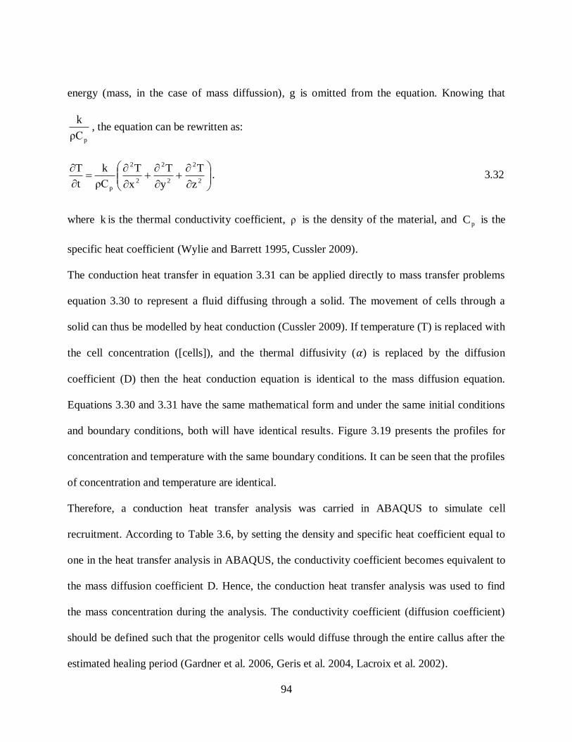
94

energy (mass, in the case of mass diffussion), g is omitted from the equation. Knowing that

pρC

k, the equation can be rewritten as:

2

2

2

2

2

2

p z

T

y

T

x

T

ρC

k

t

T. 3.32

where k is the thermal conductivity coefficient, ρ is the density of the material, and pC is the

specific heat coefficient (Wylie and Barrett 1995, Cussler 2009).

The conduction heat transfer in equation 3.31 can be applied directly to mass transfer problems

equation 3.30 to represent a fluid diffusing through a solid. The movement of cells through a

solid can thus be modelled by heat conduction (Cussler 2009). If temperature (T) is replaced with

the cell concentration ([cells]), and the thermal diffusivity ( ) is replaced by the diffusion

coefficient (D) then the heat conduction equation is identical to the mass diffusion equation.

Equations 3.30 and 3.31 have the same mathematical form and under the same initial conditions

and boundary conditions, both will have identical results. Figure 3.19 presents the profiles for

concentration and temperature with the same boundary conditions. It can be seen that the profiles

of concentration and temperature are identical.

Therefore, a conduction heat transfer analysis was carried in ABAQUS to simulate cell

recruitment. According to Table 3.6, by setting the density and specific heat coefficient equal to

one in the heat transfer analysis in ABAQUS, the conductivity coefficient becomes equivalent to

the mass diffusion coefficient D. Hence, the conduction heat transfer analysis was used to find

the mass concentration during the analysis. The conductivity coefficient (diffusion coefficient)

should be defined such that the progenitor cells would diffuse through the entire callus after the

estimated healing period (Gardner et al. 2006, Geris et al. 2004, Lacroix et al. 2002).

95

Figure 3.19. The profiles of (a) temperature and (b) fluid velocity are shown under the

same boundary condition show the same pattern (Cussler 2009).

Table 3.6. Similarity between mass diffusion and heat transfer equations.

Mass

diffusion

2

2

2

2

2

2

z

T

y

T

x

Tα

t

T Setting Dα ,

DρC

k

p

Heat transfer

2

2

2

2

2

2

z

cells

y

cells

x

cellsD

t

cells

To evaluate and validate the approach, the fluid velocity, octahedral shear strain and the

temperature (cell concentration) were predicted from the coupled diffusion-linear poroelastic

stress analysis for an axisymmetric model of a human tibia. There was no tissue differentiation

considered at this stage. The geometry, boundary conditions and mechanical load were chosen

based on a previous study and are shown in Figure 3.20a (Lacroix et al. 2002). The element type,

poroelastic and thermal material properties used in the simulation are illustrated in Table 3.7.

Fixed temperature (concentration) was imposed for each of the three origins (Figure 3.20b). The

mechanical stimuli as well as the temperature were calculated over time. The cell proliferation

was illustrated by plotting the temperature change, over time for three sample elements. The

regions closer to the temperature source (cells) had its maximum value and then diffused through

the callus over time. As an example, two plots having the bone marrow as cell origin, illustrating

the cell proliferation vs. time and cell concentration vs. distance are shown in Figure 3.21. (a)

96

Cell concentration within the callus at two time points: 0.5s and 1 s, (b) cell concentration over

time in three sample elements, (c) the cell concentration at two time points through the callus.

Figure 3.20. (a) Axisymmetric model of a human tibia, the radius of the cortical and bone

marrow are 15 and 9 mm (at the left). The cortical, bone marrow and callus are shown in

red, grey and green, respectively, (b) three origins for progenitor cells are shown. Arrows

indicate the cell origins (at the right).

Table 3.7. Element type, poroelastic and thermal properties of the tissues of a human.

tissue Element type

Poroelastic material properties Thermal properties

E [MPa] tyypermeabilik

Ns

mm4

e tyconductivik pC ρ

Cortical CAX4P 20000 0.3 0.00001 0.01 - - -

Marrow CAX4P 2 0.17 0.01 4 - - -

Callus CAX4PT 1 0.17 0.01 4 2.37 1 1

97

Figure 3.21. (a) Cell concentration within the callus at two time points: 0.5s and 1 s, (b) cell

concentration over time in three sample elements, (c) the cell concentration at two time

points through the callus.

The developed user-defined subroutine USDFLD was modified to consider the effect of

temperature (cell concentration). The material properties were updated based on the average of

computed mechanical stimuli in the previous 10 steps (days) and on the temporal and spatial

temperature (cell concentration). The utility routine GETVRM was used to call the material point

data of temperature (TEMP). The field variable as a function of temperature (cell concentration)

was obtained as follows:

10

FV...FVFVFV

1).-step(n9)-step(n10)-step(n

n ,mechanical

. 3.33

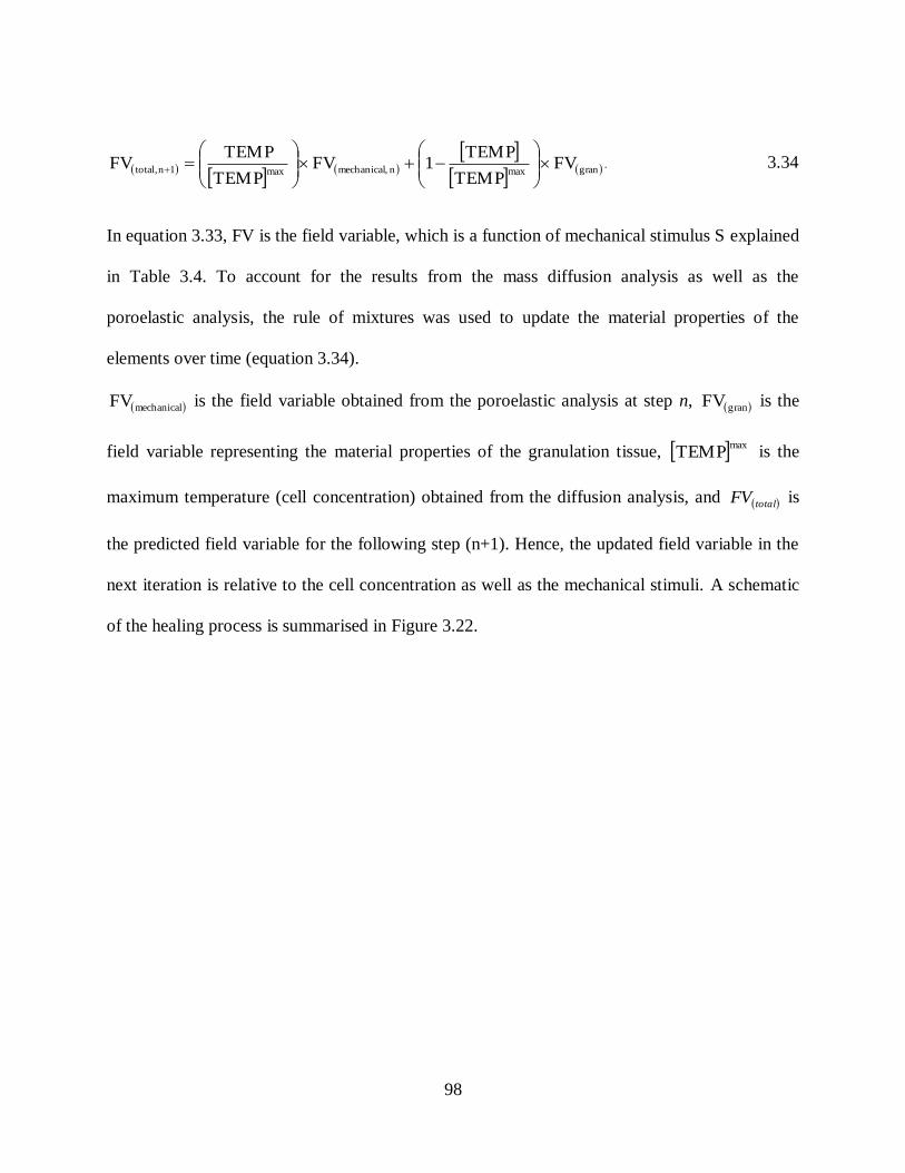
98

granmaxn ,mechanicalmax1n total, FVTEMP

TEMP1FV

TEMP

TEMPFV

. 3.34

In equation 3.33, FV is the field variable, which is a function of mechanical stimulus S explained

in Table 3.4. To account for the results from the mass diffusion analysis as well as the

poroelastic analysis, the rule of mixtures was used to update the material properties of the

elements over time (equation 3.34).

mechanicalFV is the field variable obtained from the poroelastic analysis at step n, granFV is the

field variable representing the material properties of the granulation tissue, maxTEMP is the

maximum temperature (cell concentration) obtained from the diffusion analysis, and totalFV is

the predicted field variable for the following step (n+1). Hence, the updated field variable in the

next iteration is relative to the cell concentration as well as the mechanical stimuli. A schematic

of the healing process is summarised in Figure 3.22.

99

Beginning of the differentiation(Day 1)

FEA ( ABAQUS)LoadingMaterial Properties

Biomechanical stimuli

n+1 Step (Day)

Smoothing process,New material properties(coupled poroelastic/mass diffusion analysis)

(Prendergast et al., 1997)

Figure 3.22. Schematic of the implemented algorithm to predict tissue distribution. The

coupled diffusive-poroelastic analysis for the mechanical stimulus and cell concentration

were obtained for each element (ABAQUS).

3.4 Verification of the implemented model

The FE method implemented in this study was initially verified by comparing the results to an

axisymmetric ovine tibia fracture model of Isaksson et al. (2006) with the same geometry and

loading regimes. The predicted patterns of the regenerated tissue during the repair process were

found to be very similar.

An axisymmetric FEM of an ovine tibia with a 3 mm fracture gap and external callus was

created (Figure 3.23b). An axial compression ramp load of 300 N was applied to the cortical

bone at the top of the model with the frequency of 1 Hz. The bone marrow, cortical and callus

were modelled with dimensions shown in Table 3.8. The nodes on the centre line were

constrained radially, whereas the bottom nodes were fixed vertically. Fluid was allowed to move

through and between different tissues. Based on experimental observations, the external callus is

100

impermeable. Therefore, there was no fluid exudation from external boundaries (Isaksson et al.

2006).

As explained in the previous section, the biphasic theory regulated by shear strain and fluid flow

was implemented into our simulation to investigate the tissue differentiation over healing time

(Prendergast et al. 1997). It was assumed that the callus consisted of stem cell seeded granulation

tissue initially, and cells could differentiate into fibrous tissue, immature and mature cartilage,

immature and mature bone. The tissue material properties can be found in Table 3.3. Progenitor

cells from three origins were able to move into the callus (Figure 3.20b). Cell migration and

proliferation were modelled as a diffusion process, coupled to the tissue-deformation stress

analysis. The diffusion coefficients were set such that after 6 weeks, the progenitor cells could

spread throughout the entire callus (Lacroix et al. 2002). A coupled diffusion-poroelastic analysis

was modelled. The model was meshed and the number of elements in the callus, bone marrow

and orti al one were ompared with Isaksson‟s model (Table 3.8).

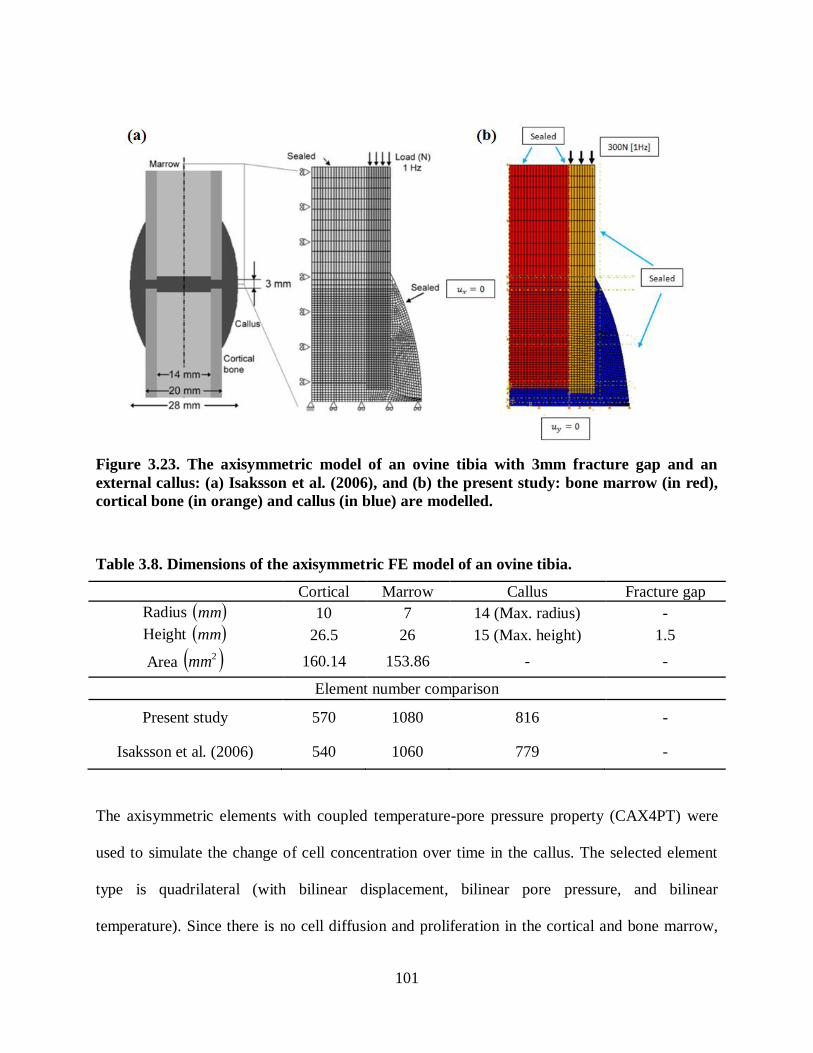
101

Figure 3.23. The axisymmetric model of an ovine tibia with 3mm fracture gap and an

external callus: (a) Isaksson et al. (2006), and (b) the present study: bone marrow (in red),

cortical bone (in orange) and callus (in blue) are modelled.

Table 3.8. Dimensions of the axisymmetric FE model of an ovine tibia.

Cortical Marrow Callus Fracture gap

Radius mm 10 7 14 (Max. radius) -

Height mm 26.5 26 15 (Max. height) 1.5

Area 2mm 160.14 153.86 - -

Element number comparison

Present study 570 1080 816 -

Isaksson et al. (2006) 540 1060 779 -

The axisymmetric elements with coupled temperature-pore pressure property (CAX4PT) were

used to simulate the change of cell concentration over time in the callus. The selected element

type is quadrilateral (with bilinear displacement, bilinear pore pressure, and bilinear

temperature). Since there is no cell diffusion and proliferation in the cortical and bone marrow,

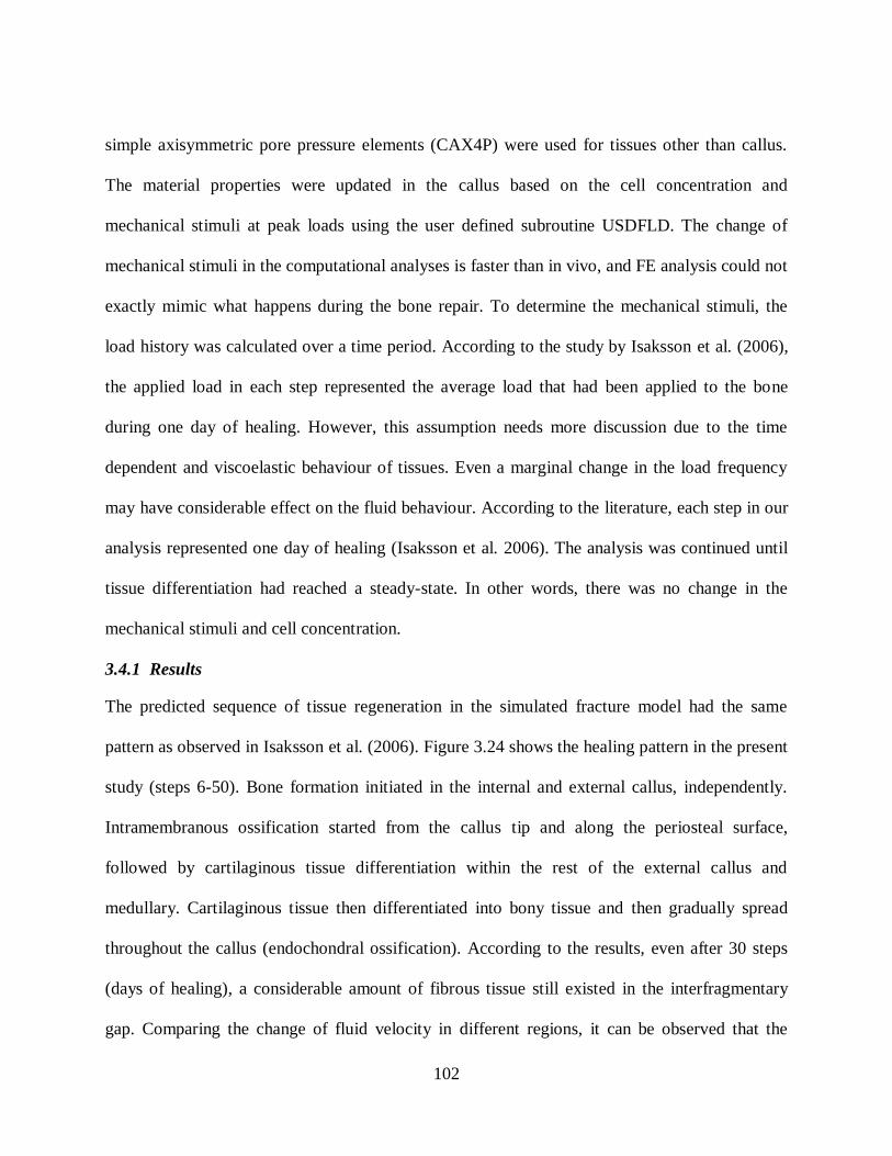
102

simple axisymmetric pore pressure elements (CAX4P) were used for tissues other than callus.

The material properties were updated in the callus based on the cell concentration and

mechanical stimuli at peak loads using the user defined subroutine USDFLD. The change of

mechanical stimuli in the computational analyses is faster than in vivo, and FE analysis could not

exactly mimic what happens during the bone repair. To determine the mechanical stimuli, the

load history was calculated over a time period. According to the study by Isaksson et al. (2006),

the applied load in each step represented the average load that had been applied to the bone

during one day of healing. However, this assumption needs more discussion due to the time

dependent and viscoelastic behaviour of tissues. Even a marginal change in the load frequency

may have considerable effect on the fluid behaviour. According to the literature, each step in our

analysis represented one day of healing (Isaksson et al. 2006). The analysis was continued until

tissue differentiation had reached a steady-state. In other words, there was no change in the

mechanical stimuli and cell concentration.

3.4.1 Results

The predicted sequence of tissue regeneration in the simulated fracture model had the same

pattern as observed in Isaksson et al. (2006). Figure 3.24 shows the healing pattern in the present

study (steps 6-50). Bone formation initiated in the internal and external callus, independently.

Intramembranous ossification started from the callus tip and along the periosteal surface,

followed by cartilaginous tissue differentiation within the rest of the external callus and

medullary. Cartilaginous tissue then differentiated into bony tissue and then gradually spread

throughout the callus (endochondral ossification). According to the results, even after 30 steps

(days of healing), a considerable amount of fibrous tissue still existed in the interfragmentary

gap. Comparing the change of fluid velocity in different regions, it can be observed that the

103

maximum fluid velocity is 0.23 [ m/s] at the tip of external callus, however it is around 12 times

larger under the cortical shaft (2.84 [ m/s]) during healing (Figure 3.25). Therefore, high

magnitudes of fluid velocity may be the result of delayed tissue differentiation. Since axial

compressive load had been applied to the cortical shaft, the zones in the interfragmentary gap

(under the cortical shaft) experienced higher load magnitudes and thus fluid velocity had

increased.

The predicted tissue distributions were compared with those obtained by Isaksson et al. (2006)

(Figure 3.26-28). As presented in Figure 3.26, fibrous tissue was surrounded by cartilage under

the cortical shaft. In addition, intramembranous ossification occurred in the external callus at the

callus tip and along the periosteum at the beginning of the analysis in both models. After 50

steps, a marginable amount of fibrous tissue, surrounded by mature cartilaginous tissue, exists at

the fracture gap. However, the rest of callus was filled with intermediate and/or mature bony

tissue. Mature bone was observed in most parts of the external callus. Intermediate bone exists at

the bottom right side of the external callus and at left corner of internal callus (Figure 3.26 and

Figure 3.27).

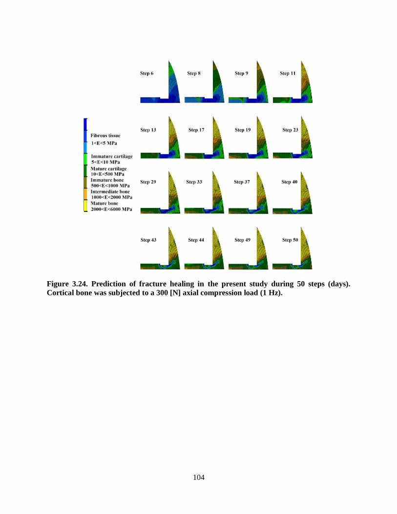
104

Figure 3.24. Prediction of fracture healing in the present study during 50 steps (days).

Cortical bone was subjected to a 300 [N] axial compression load (1 Hz).

105

Figure 3.25. The change of fluid flow [ m/s] over time under the cortical shaft and callus

tip during fracture healing. Cortical bone was subjected to a 300 N axial compression

loading (1 Hz).

Figure 3.26. Comparison of the two simulations during fracture healing in the first steps.

Cortical bone was subjected to a 300 N axial compression loading (1 Hz): (a) the present

study, and (b) Isaksson et al. (2006). In both models, intramembranous ossification

occurred at the callus tip and periosteum. Also, fibrous tissue and cartilaginous tissue can

be found in the same zones.

106

Figure 3.27. Comparison of the two simulations during fracture healing at step 50, cortical

bone was under 300 N axial compression loading (1 Hz): (a) the present study, (b) Isaksson

et al. (2006). The amount of fibrous tissue decreased significantly under the cortical shaft.

The distribution of mature and intermediate bone distribution is almost identical.

107

Step 9

Step 13

Step 23

Step 33

Step 50

(a) (b)

(a)

(b)

Figure 3.28. Overall similar healing patterns were observed over time under a 300 [N] axial

compression load in (a) the present study, and (b) Isaksson et al. (2006).

3.4.2 Discussion

The temporal and spatial tissue differentiation in Isaksson et al. (2006) and the present study

were quite similar, but not exactly the same (Figure 3.28). The minor differences may be due to

the different method of implementing the mass diffusion analysis. In the previous study done by

Isaksson et al. (2006), MATLAB was linked to ABAQUS in order to update the element material

108

properties (Lacroix et al. 2002, Sandino and Lacroix 2011) whereas in this study a user defined

subroutine was written in FORTRAN. In Isaksson et al. (2006), the values of Young‟s modulus,

oisson‟s ratio and permea ility were averaged separately in MATLAB to predict the tissue

type. However, in this study, all of the material properties were obtained through the field

variable and by determining the FV in each step, the material properties were updated

automatically, slightly differently, through FV.

Isaksson et al. (2006) used a diffusion process uncoupled to the tissue poroelastic analysis.

Moreover, the eight-node element with 9 integration points was used (CAX8P). However, in this

study a fully coupled diffusion-poroelastic analysis was performed. Due to the available coupled

temperature-pore pressure elements in ABAQUS v6.10, a four-node axisymmetric quadrilateral

elements with 4 integration points (CAX4PT) was used for the callus, and a four-node

axisymmetric element with 4 integration points was used for bone marrow and cortical

(CAX4P).

Despite these differences in model implementation, the predicted tissue differentiation for both

models was very similar. Hence, the current model can be considered verified against Isaksson et

al. (2006) and we were confident in implementing the method into our FE models of murine tibia

and investigating the effect of mechanical loading on tissue differentiation and bone repair.

3.5 Fracture healing case studies

The mechanoregulatory algorithm was implemented into an idealised models of a murine tibia.

First, an axisymmetric model was simulated to investigate the effect of load magnitude on

fracture healing. Second, a three dimensional (3D) model was created to determine the effect of

torsional load as well as combined loading on the temporal and spatial differentiation patterns.

109

3.5.1 An axisymmetric idealized murine model

An axisymmetric FE model of a proximal section of a murine tibia with a 0.4 mm fracture gap

and external callus were created based on the described method in the previous sections (Figure

3.29a). The mid-diaphyseal dimensions of the modelled murine tibia are shown in Table 3.9

(Windahl et al. 1999, Geris et al. 2004). To investigate the influence of load magnitude on

fracture repair, axial compression loads of 0.5, 1, 2 N (1 Hz) were applied to the top of the

cortical shaft (Figure 3.29b). Verification of the results was done by comparing to CT images

of a previously published experimental study (Gardner et al. 2006).

Figure 3.29. (a) Axisymmetric FE model of a murine tibia (bone marrow in red, cortical

bone in grey and callus in blue), (b) the amplitude of the applied cyclic axial compression

loads.

Tissues were assumed to follow the biphasic algorithm proposed by Prendergast et al. (1997) and

the material properties were set as described in Table 3.10. The Young‟s modulus, oisson‟s

ratio, permeability and the void ratio were defined for each tissue. Cortical bone has the highest

110

stiffness. However, it has the lowest permeability due to a low void ratio of 0.0416. Immature,

intermediate and mature woven bones were modelled to represent the tissue differentiation over

time. The Young‟s modulus of immature, intermediate and mature woven one are 500<E<1000

MPa, 1000<E<2000 MPa, and from 2000<E<6000 MPa, respectively. Mature and immature

cartilage were also modelled with the Young‟s modulus of 10<E<500 and 5<E<10, respe tively.

Finally, the Young‟s modulus of fi rous tissue ranged between 1 and 5 MPa. The material

properties used in this study can be found in Table 3.10.

Table 3.9. Geometry of the murine tibia proximal section (Windahl et al. 1999, Geris et al.

2004).

Cortical periosteal circumference mm 4.51

Cortical endosteal circumference mm 3.12

Maximum external callus radius mm 1.2

Fracture gap mm 0.4

The boundary conditions were set such that the nodes located on the symmetry axis are

constrained in the x-direction and the bottom of the model in the y-direction. The external

boundaries were assumed to be impermeable. All tissues were modelled using pore pressure

elements. The bone marrow and cortical bone contained 444 and 240 simple axisymmetric pore

pressure (CAX4P) elements, and the callus was meshed using 480 axisymmetric temperature-

pore pressure elements (CAX4PT).

It was assumed that a fixed number of progenitor cells originated from the bone marrow,

periosteum and surrounding muscle tissues and were able to move within the callus. The

diffusion coefficient set such that after 3 weeks, the progenitor cells would have spread

throughout the callus (Gardner et al. 2006).

111

The mechanical stimuli (fluid velocity and tissue octahedral shear strain) and the cell

concentration were computed at the callus elements (at maximum loading) by implementing a

coupled diffusive-poroelastic analysis. The geometric nonlinearity (NLGEOM) option in

ABAQUS was switched on in order to account for large deformations in the tissues.

Table 3.10. Material properties used for the study (Rho, Ashman and Turner 1993,

Isaksson et al. 2006).

Constant Variable

Cortical Marrow Granulation

tissue

Fibrous

tissue Cartilage

Immature

bone

Mature

bone ovine tibia

E [GPa] 6 0.002 0.0002 310- 3105

3105 -

0.5 0.5-1 2-6

0.325 0.167 0.167 0.167 0.167 0.325 0.325

k

Ns

mm 4

510 0.010 0.010 0.010 0.005 0.100 0.370

e 0.041 4.00 4.00 4.00 4.00 4.00 4.00

According to the obtained mechanical stimuli and cell concentration, the material properties of

the cells within the callus elements were updated using a rule of mixtures (equation 3.34). The

callus cells within an element differentiated into fibrous tissue, mature and immature cartilage

and mature, intermediate and immature woven bone. There was no tissue differentiation within

the marrow and cortical bone. Therefore, the material properties of marrow and cortical bone

were kept constant over time. The analysis continued until steady-state was reached.

3.5.1.1 Results

Bone formation was successfully simulated over time with the sequential prediction of fibrous,

cartilage and mature bony tissue. The predicted sequence of tissue regeneration in the murine

112

fracture model occurred in the same pattern observed in vivo (Figure 3.30). In all cases, the bone

formation started from the internal and external callus, independently. For the external callus, the

bone formation started at the tip of the callus and gradually spread throughout the callus. First,

cartilaginous tissue formed and then differentiated into bony tissue. The interfragmentary

movement was computed for all cases. Under the 0.5 N loading case the interfragmentary

movement was negligible after 10 steps. However, for 1 N and 2 N the movement decreased to

0.04 mm and 0.07 mm. The fluid velocity and strain were reduced over time, which illustrates

that the callus became stiffer over time. For the 0.5 N loading case, the mechanical stimuli had

less magnitude and reached a steady state faster than higher load magnitudes (Figure 3.31). After

14 steps (days), the interfragmentary gap still contained fibrous tissue for the load amplitudes of

1 or 2 N whereas cartilage was predicted for the 0.5 N loading case (Figure 3.30). According to

the obtained results, the bone healing rate was the highest under 0.5 N, intermediate under 1 N

and lowest under 2 N axial compression, which corresponded to in vivo observations.

Figure 3.30. Predicted tissue differentiation in the present study under (a) 0.5 N, (b) 1 N

and (c) 2 N axial compression load (1 Hz).

113

0

10

20

30

40

50

0 5 10 15 20

Oct

ahed

ral s

hea

r st

rain

[%

]

Step (day)

0.5 N 1 N 2 N

0

1

2

3

4

5

6

0 5 10 15 20

Flu

id v

elo

ciy

[µm

/s]

Step (day)

0.5 N 1 N 2 N

Figure 3.31. Predicted mechanical stimuli for a sample element under the cortical shaft

during the healing process for three axial compression loading magnitudes.

3.5.1.2 Discussion

The bone under higher mechanical conditions had higher interfragmentary movement and higher

fluid velocity. The higher magnitude of movement led to instability and a delay in bone healing.

The computational results were compared with a previous experimental study (Gardner et al.

2006). The murine bones had a similar fracture size and were under identical mechanical

conditions in both cases. In agreement with the micro-CT images from Gardner et al. (2010), the

computational simulations predicted bone repair enhancement under low magnitudes of load

(Figure 3.32c). As seen in Figure 3.30 the bone under 0.5 N had stiffer bridging. Octahedral

shear strain magnitudes were higher in the 2 N case, which led to less consolidation and fibrous

tissue was still observed after 2 weeks (Figure 3.32b). At higher loads the callus was poorly

bridged as seen in the CT images (Figure 3.32c).

114

Figure 3.32. a) Axisymmetric FE model of a murine tibia. The inner and outer diameter of

cortical bone (gray) and external callus (blue) are 1, 1.5 and 2.4 mm, respectively, b)

Predicted tissue differentiation in the present study, c) CT images from Gardner et al.

(2006) for different load magnitudes (1 Hz).

3.5.2 A 3D idealised model of murine tibia

Since axial torsion could not been applied to the 2D model, a poroelastic three-dimensional (3D)

finite element model of a murine ti ia with a 0.4 mm gap and external allus was reated

(ABAQUS v6.10). In order to be able to apply torsional load, a 3D model was created (Figure

3.35a). To decrease the computational cost, a 22.5 degree wedge was modelled. The boundary

conditions were chosen so that the bottom surface was fixed in axial and angular directions and

the vertical axis at the left was restricted radially. The bone marrow and cortical bone contained

759 and 432 simple three dimensional 8-node trilinear displacement and pore pressure (C3D8P)

elements, and the callus was meshed using 949 three dimensional 8-node trilinear displacement,

pore pressure, and temperature elements (C3D8PT). The external surface of the callus and

external surfaces of the bone were assumed to be impermeable. The NLGEOM option in

ABAQUS was switched on to consider geometric nonlinearity in the tissues. The diffusion

115

coefficient was set such that, after 3 weeks, the mesenchymal stem cells would spread

throughout the callus (Gardner et al. 2006). It was assumed that initially the callus consisted of

stem cell seeded granulation tissue. Murine embryonic stem cells were transplanted due to their

regenerative capacity. The elements within the callus were able to differentiate into fibrous

tissue, immature and mature cartilage, and immature, intermediate and mature bony tissue.

Progenitor cells migrated into the callus from surrounding tissues, marrow, periosteum and

external soft tissues. To investigate the influence of mechanical environments, axial torsion (8

degrees, 1 Hz) alone, and then combined, axial compression (0.4 N, 1 Hz) and torsion (8 degrees,

1 Hz) were applied to the cortical shaft with a maximum octahedral shear strain magnitude of 25

%, based on a previous in vivo study (Bishop et al. 2006). In the experimental study, cyclic axial

torsion was applied over a fractured sheep tibia with a maximum principal strain of 25 %

(Bishop et al. 2006).

3.5.2.1 Results

The predicted sequence of tissue differentiation in the 3D murine fracture model occurred as

expected in both cases. First, the granulation tissue differentiated into cartilaginous tissue which

was initiated from the callus tip at a faster pace. The bony tissue, formed from cartilage

(endochondral ossification), was first observed in the external callus and then spread throughout

the callus gradually. As expected, fibrous tissue existed in the medullary cavity even after 15

days of healing. The interfragmentary movement decreased with healing in both cases.

For the axial torsion case, the magnitude of octahedral shear strain and fluid velocity were

plotted over time for three sample elements located in the external callus, interfragmentary

region and internal callus (Figure 3.34). As seen in Figure 3.34, the element under the cortical

shaft has the highest mechanical stimuli. The strain reaches 6 % under the cortical bone, whereas

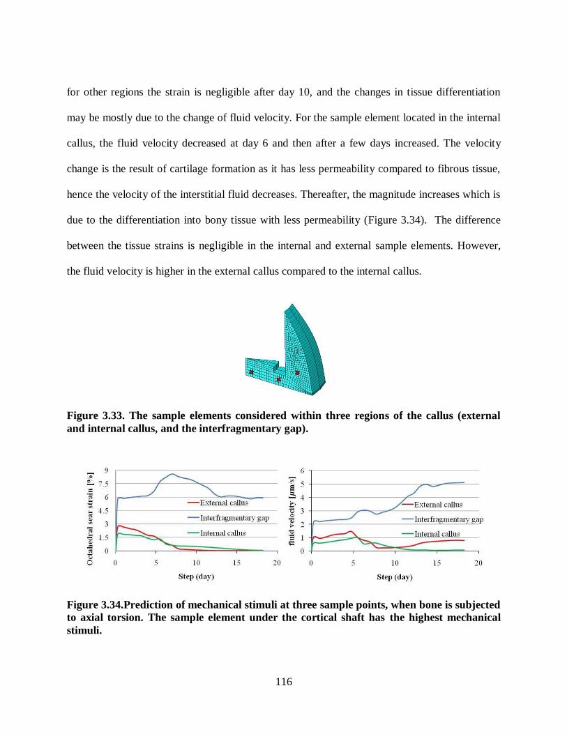
116

for other regions the strain is negligible after day 10, and the changes in tissue differentiation

may be mostly due to the change of fluid velocity. For the sample element located in the internal

callus, the fluid velocity decreased at day 6 and then after a few days increased. The velocity

change is the result of cartilage formation as it has less permeability compared to fibrous tissue,

hence the velocity of the interstitial fluid decreases. Thereafter, the magnitude increases which is

due to the differentiation into bony tissue with less permeability (Figure 3.34). The difference

between the tissue strains is negligible in the internal and external sample elements. However,

the fluid velocity is higher in the external callus compared to the internal callus.

Figure 3.33. The sample elements considered within three regions of the callus (external

and internal callus, and the interfragmentary gap).

Figure 3.34.Prediction of mechanical stimuli at three sample points, when bone is subjected

to axial torsion. The sample element under the cortical shaft has the highest mechanical

stimuli.

117

The mechanical stimuli had higher magnitudes when the bone was under combined loading

compared to the torsion alone case. Under pure axial torsion, bony tissue was also formed in the

internal callus. In addition, there were greater bony areas and density. However, under combined

loading, only cartilaginous tissue was observed in the internal region and no bone had

regenerated. The algorithm predicted stiffer bridging and promoted healing in pure torsion

(Figure 3.35b). Whereas, poorly bridged callus and promoted healing were predicted with added

axial compression (Figure 3.35c).

Figure 3.35. (a) A 3D FEM of a murine tibia with 0.4 mm gap, predicted tissue

differentiation in the model under: (b) Axial torsion (8 degree, 1 Hz), (c) Axial torsion &

compression (8 degrees, 0.45 MPa, 1 Hz).

3.5.2.2 Discussion

Fibrous tissue was still present under the cortical shaft after 2 weeks of healing, which may be

related to the higher magnitudes of fluid velocity at the interfragmentary gap compared to other

regions. The algorithm predicted stiffer bridging and promoted better healing in torsion

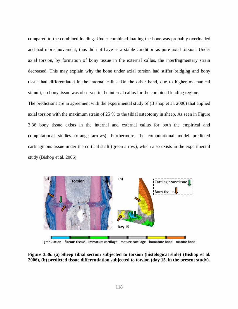
118

compared to the combined loading. Under combined loading the bone was probably overloaded

and had more movement, thus did not have as a stable condition as pure axial torsion. Under

axial torsion, by formation of bony tissue in the external callus, the interfragmentary strain

decreased. This may explain why the bone under axial torsion had stiffer bridging and bony

tissue had differentiated in the internal callus. On the other hand, due to higher mechanical

stimuli, no bony tissue was observed in the internal callus for the combined loading regime.

The predictions are in agreement with the experimental study of (Bishop et al. 2006) that applied

axial torsion with the maximum strain of 25 % to the tibial osteotomy in sheep. As seen in Figure

3.36 bony tissue exists in the internal and external callus for both the empirical and

computational studies (orange arrows). Furthermore, the computational model predicted

cartilaginous tissue under the cortical shaft (green arrow), which also exists in the experimental

study (Bishop et al. 2006).

Figure 3.36. (a) Sheep tibial section subjected to torsion (histological slide) (Bishop et al.

2006), (b) predicted tissue differentiation subjected to torsion (day 15, in the present study).

119

3.6 Summary of the computational analyses

The verified algorithm was implemented into two idealised murine models and the effects of

mechanical loading on the healing process were investigated:

1. A poroelastic two dimensional (2D) FE model of a murine tibia with a 0.4 mm gap and

external callus was created (ABAQUS v6.11). To explore the influence of load

magnitude on fracture repair, axial compression loads of 0.5, 1, 2 N (1 Hz) were applied

to the top of the cortical shaft, and the results were compared to reconstructed µCT

images of a previously published experimental study (Gardner et al. 2006).

2. A poroelastic idealised three-dimensional (3D) FE model of a murine tibia with a 0.4 mm

gap and external callus was created (ABAQUS v6.11). To investigate the influence of

mechanical environments, axial compression (0.4 N, 1 Hz) and torsional rotation (8

degrees, 1 Hz), were applied to the cortical shaft with a maximum octahedral shear strain

magnitude of 25 %. The predictions agreed with the experimental study of Bishop et al.

(2006) that applied axial torsion with the maximum strain of 25 % to the tibial osteotomy

in sheep.

The first specific objective of the study was to investigate the mechanical environments within a

stem cell collagenous scaffold (Chapter 4):

1. An axisymmetric FE model of the modified Flexcell system was created to apply

confined compression test, using ABAQUS v6.11.

2. The load-deflection FE results for the rate of 1 N/s were validated against the preliminary

experimental results from our group (Olesja Hazenbiller, University of Calgary, M.Sc.

student).

120

3. The biphasic algorithm was implemented into the computational model to predict tissue

differentiation under confined compression (5 and 20 kPa, 1 Hz). In agreement with our

experimental results, gel became stiffer by differentiating into cartilaginous tissues

(Olesja Hazenbiller, University of Calgary, M.Sc. student).

The second specific objective was to simulate tissue differentiation within a µCT-based FE

model of a murine tibia (Chapter 5):

1. The µCT based FE model of a burr-hole murine tibia was reconstructed using

Simpleware software. The non-homogeneous grey-scale based mechanical properties

were used.

2. The mechanical behaviour of the reconstructed model was verified against the published

experimental study of Stadelmann et al. (2009). Octahedral shear strain was estimated

numerically in three different zones of the murine tibia and compared with the available

empirical results. The computational and empirical results were in good agreement

qualitatively.

3. The biphasic algorithm was implemented into the computational model to predict the

development of differentiated tissues in a closed fracture model treated with a stem cell

seeded soft collagenous scaffold: (1) under different loading conditions (e.g. axial

compression and bending), (2) for different locations of the scaffold, and (3) different

rates of diffusion.

The following figure summarizes the computational simulations conducted in this thesis (3.37).

121

Figure 3.37. Summary of the computational simulations in the current study.

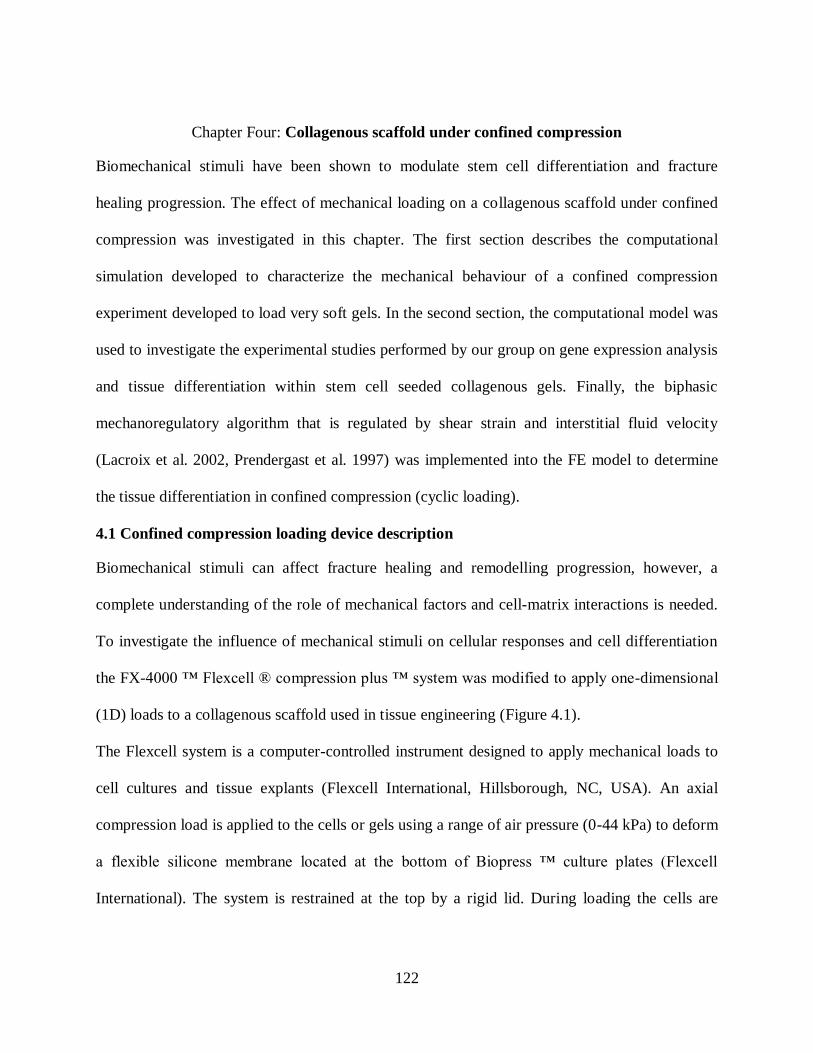
122

Chapter Four: Collagenous scaffold under confined compression

Biomechanical stimuli have been shown to modulate stem cell differentiation and fracture

healing progression. The effect of mechanical loading on a collagenous scaffold under confined

compression was investigated in this chapter. The first section describes the computational

simulation developed to characterize the mechanical behaviour of a confined compression

experiment developed to load very soft gels. In the second section, the computational model was

used to investigate the experimental studies performed by our group on gene expression analysis

and tissue differentiation within stem cell seeded collagenous gels. Finally, the biphasic

mechanoregulatory algorithm that is regulated by shear strain and interstitial fluid velocity

(Lacroix et al. 2002, Prendergast et al. 1997) was implemented into the FE model to determine

the tissue differentiation in confined compression (cyclic loading).

4.1 Confined compression loading device description

Biomechanical stimuli can affect fracture healing and remodelling progression, however, a

complete understanding of the role of mechanical factors and cell-matrix interactions is needed.

To investigate the influence of mechanical stimuli on cellular responses and cell differentiation

the FX-4000 ™ Flex ell ® ompression plus ™ system was modified to apply one-dimensional

(1D) loads to a collagenous scaffold used in tissue engineering (Figure 4.1).

The Flexcell system is a computer-controlled instrument designed to apply mechanical loads to

cell cultures and tissue explants (Flexcell International, Hillsborough, NC, USA). An axial

compression load is applied to the cells or gels using a range of air pressure (0-44 kPa) to deform

a flexi le sili one mem rane lo ated at the ottom of iopress ™ ulture plates (Flex ell

International). The system is restrained at the top by a rigid lid. During loading the cells are

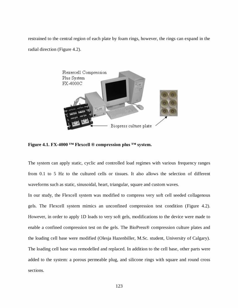
123

restrained to the central region of each plate by foam rings, however, the rings can expand in the

radial direction (Figure 4.2).

Figure 4.1. FX-4000 ™ Fl xc ll ® comp ssion pl s ™ sys m.

The system can apply static, cyclic and controlled load regimes with various frequency ranges

from 0.1 to 5 Hz to the cultured cells or tissues. It also allows the selection of different

waveforms such as static, sinusoidal, heart, triangular, square and custom waves.

In our study, the Flexcell system was modified to compress very soft cell seeded collagenous

gels. The Flexcell system mimics an unconfined compression test condition (Figure 4.2).

However, in order to apply 1D loads to very soft gels, modifications to the device were made to

enable a confined compression test on the gels. The BioPress® compression culture plates and

the loading cell base were modified (Olesja Hazenbiller, M.Sc. student, University of Calgary).

The loading cell base was remodelled and replaced. In addition to the cell base, other parts were

added to the system: a porous permeable plug, and silicone rings with square and round cross

sections.

124

The modified system contains seven parts: (1) the flexible membrane, (2) modified cell base, (3)

collagen gel, (4) square ring, (5) porous plug, (6) round ring, and (7) the top lid. The parts added

to the system are presented in Figure 4.3.

Figure 4.2. Schematic of the Flexcell system cross-section in the uncompressed and

compressed configurations.

A 316L stainless steel (SS) porous plug with 10 µm pore size is used to permit nutrient and

oxygen exchange as well as provide a rigid surface to transfer loads (MOTT Corporation,

Farmington, CT, USA). It has been shown that the 316L SS plug has appropriate

biocompatibility for short term and long term cell cultures (Jacobs and Oloff 1985, Puleo et al.

1991). The plug allows for fluid exudation from the top surface, and also enables the exchange of

oxygen needed for cell culture in an incubator. Moreover, the plug has similar physical

properties to (mature) trabecular bone with approximately similar porosity properties (Wen

2009).

125

Figure 4.3. Parts of the modified system: (1) cell base, (2) square ring, (3) porous plug, (4)

round ring, (5) lid, and (6) fixed lid.

Silicone rings possess good biocompatibility and thus are used in implants and prostheses,

gaskets, seals and O-rings (Schulmerich et al. 2006). The silicone rings used in our experiments

have a good resistance to chemical and biological degradation. The silicone ring with a circular

cross section was used to bridge the gap between the plug and the top lid, and maintain contact

between the porous plug and the fixed lid. There were three main reasons for adding the square

ring to the system:

(1) The collagen gel had very low stiffness and could not maintain its shape; therefore, the

silicone square ring acted as a support for the soft gel in a 1D configuration; (2) it was used to

ensure the loading conditions were predominantly 1D, and (3) during the loading and unloading

period, it was used to maintain the gel within the loading device. The schematic of the system is

presented in Figure 4.4 and 4.5.

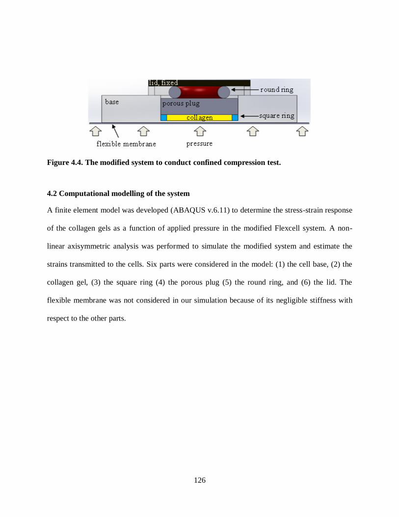
126

Figure 4.4. The modified system to conduct confined compression test.

4.2 Computational modelling of the system

A finite element model was developed (ABAQUS v.6.11) to determine the stress-strain response

of the collagen gels as a function of applied pressure in the modified Flexcell system. A non-

linear axisymmetric analysis was performed to simulate the modified system and estimate the

strains transmitted to the cells. Six parts were considered in the model: (1) the cell base, (2) the

collagen gel, (3) the square ring (4) the porous plug (5) the round ring, and (6) the lid. The

flexible membrane was not considered in our simulation because of its negligible stiffness with

respect to the other parts.

127

Figure 4.5. The parts added to the modified Flexcell system.

4.2.1 The cell base and the top lid

The cell base and the top lid were modelled as analytical rigid shells due to their high stiffness

compared to the other parts. Analytical rigid surfaces are geometric surfaces that can be

described by straight and curved line segments, and their motion is defined through a single node

with six degrees of freedom (i.e., a rigid body reference node). The reference points were

positioned at the centre of mass for both parts. An axial compression force was applied to the

reference node of the cell base at the bottom while a fixed boundary condition was implemented

at the top lid. Assuming the base and the lid to be rigid bodies improved computational time

without affecting the overall accuracy of the analysis.

4.2.2 The collagen gel and the porous plug

The material properties of the collagenous soft gel were considered to be similar to granulation

tissue with a Young‟s modulus of 0.2 M a and a oisson‟s ratio of 0.167 and a permea ility of

128

0.01 Ns

mm 4

. The Young‟s modulus of the gel was also determined (approximately 0.15 MPa)

from the stress-strain curve obtained experimentally (Olesja Hazenbiller, M.Sc. student,

University of Calgary). The collagen gel was modelled as a biphasic material (80 % fluid and 20

% solid). The void ratio (e) was set to 4 and meshed using continuum eight-node axisymmetric

pore pressure elements (CAX8P).

A 3.3175 mm thick 316L stainless steel porous plug with a 12.7-mm-diameter was created. It

was also modelled as a biphasic material. The permeability of a 316L stainless steel plug with a

0.5 µm pore size was reported to be close to the permeability of the cortical bone (510

Ns

mm 4

)

(Wen 2009). Since the porous plug that we used had much higher pore size (10 µm), the

permeability of the plug was set close to the permeability of mature trabecular bone with the

value of 0.37 Ns

mm 4

. The void ratio was calculated from the geometry and the density. Knowing

the mass and density of the plug

3cm

gr7.99ρ1.031gr,m the volume would be:

3

solid cm0.254ρ

mV . 4.1

The volume could also be determined from the radius and the height of the plug. For a height

(h=0.125 in) and a radius (r=0.25 in) the volume would be:

32

total cm0.402hπrV . 4.2

The difference between these volumes established the void volume ( 3

f 0.148cmV ). Therefore,

the void ratio of the porous plug was computed and used in the computational simulation:

129

0.582V

Ve

s

f

. 4.3

The void ratio of the plug (e = 0.582) was 7 times less than the trabecular bone (e = 4.0). The

values for Young‟s modulus, oisson‟s ratio, permea ility and void ratio of the ollagen gel and

the porous plug used in the model can be found in Table 4.1.

Table 4.1. Poroelastic properties of the porous plug and the collagen gel (Isaksson et al.

2006, Tromas et al. 2012).

E MPa k

Ns

mm 4

e

Porous plug 193000 0.30 0.37 0.582

Collagenous gel 0.2 0.167 0.01 4.0

4.2.3 The silicone rings

The silicone rings were modelled as isotropic hyperelastic materials and meshed using eight-

node axisymmetric quadrilateral elements with hybrid formulation (CAX8H). The hybrid

elements were used to consider the incompressibility of the silicone rings. The geometry of the

rings is provided in Table 4.2.

Hyperelastic materials are described in terms of the strain energy stored in the material per unit

volume (i.e. strain energy potential). The derivative of the strain energy function with respect to

a strain component determines the corresponding stress component. The stress-strain data

obtained from a uniaxial compression test (Olesja Hazenbiller, M.Sc. student, University of

Calgary) was used as material input into ABAQUS v6.11

The strain energy potential (W) is defined as follows in the Marlow form, which is suited for

quasi-incompressible materials. Also, for the cases in which only one set of data is available

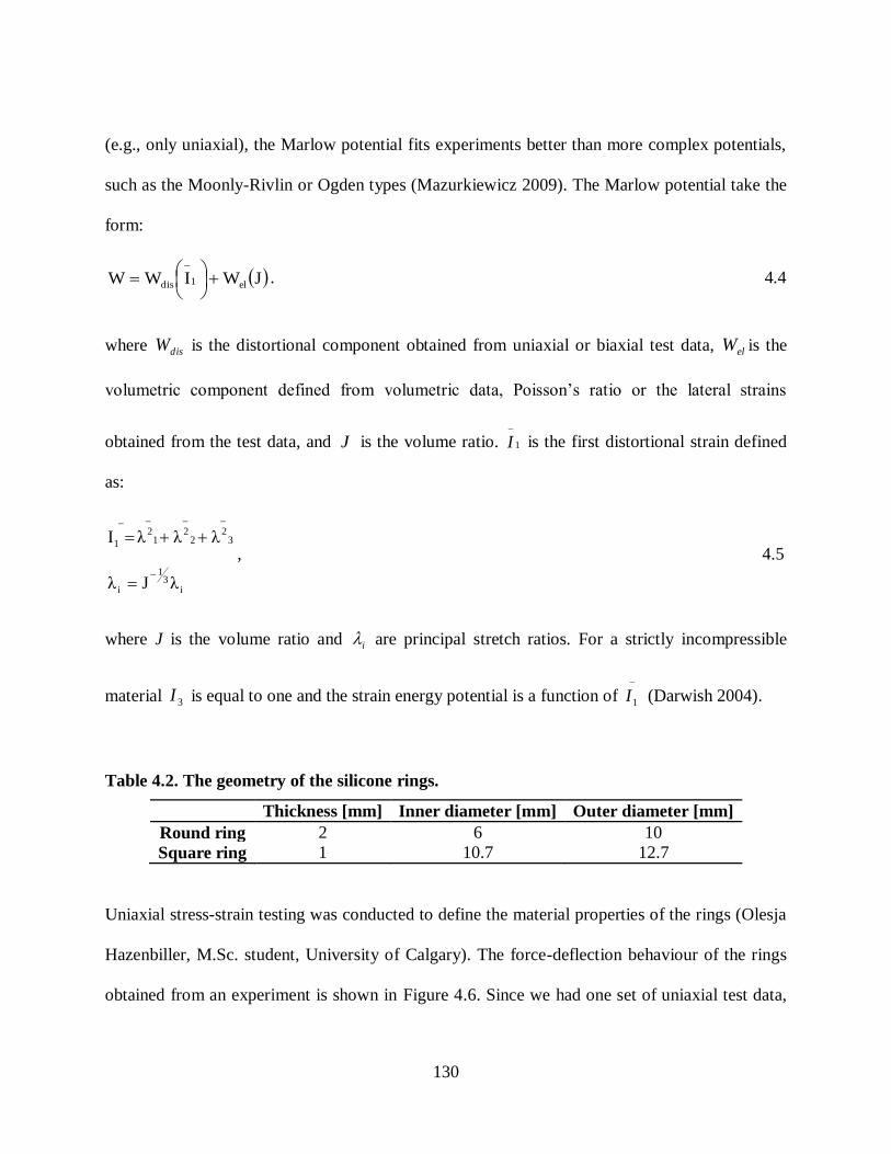
130

(e.g., only uniaxial), the Marlow potential fits experiments better than more complex potentials,

such as the Moonly-Rivlin or Ogden types (Mazurkiewicz 2009). The Marlow potential take the

form:

JWIWW el1dis

. 4.4

where disW is the distortional component obtained from uniaxial or biaxial test data, elW is the

volumetri omponent defined from volumetri data, oisson‟s ratio or the lateral strains

obtained from the test data, and J is the volume ratio. 1

I is the first distortional strain defined

as:

i3

1

i

32

22

12

1

λJλ

λλλI

, 4.5

where J is the volume ratio and i are principal stretch ratios. For a strictly incompressible

material 3I is equal to one and the strain energy potential is a function of

1I (Darwish 2004).

Table 4.2. The geometry of the silicone rings.

Thickness [mm] Inner diameter [mm] Outer diameter [mm]

Round ring 2 6 10

Square ring 1 10.7 12.7

Uniaxial stress-strain testing was conducted to define the material properties of the rings (Olesja

Hazenbiller, M.Sc. student, University of Calgary). The force-deflection behaviour of the rings

obtained from an experiment is shown in Figure 4.6. Since we had one set of uniaxial test data,

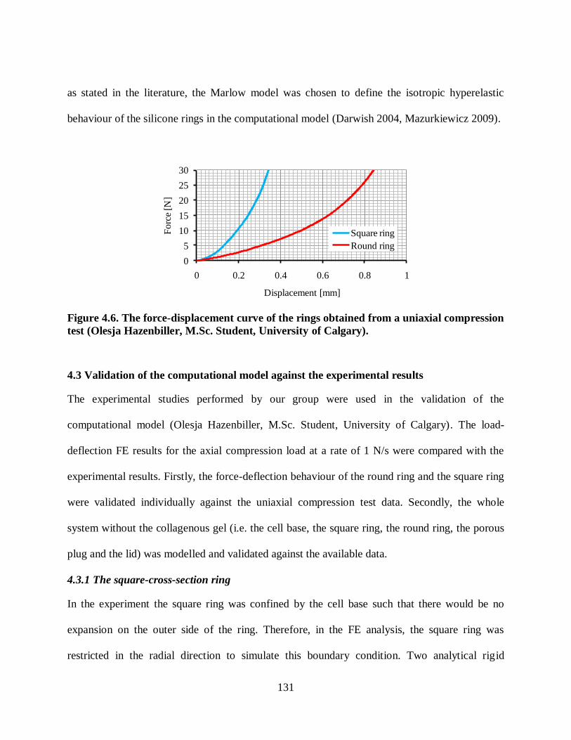
131

as stated in the literature, the Marlow model was chosen to define the isotropic hyperelastic

behaviour of the silicone rings in the computational model (Darwish 2004, Mazurkiewicz 2009).

0

5

10

15

20

25

30

0 0.2 0.4 0.6 0.8 1

Fo

rce

[N]

Displacement [mm]

Square ring

Round ring

Figure 4.6. The force-displacement curve of the rings obtained from a uniaxial compression

test (Olesja Hazenbiller, M.Sc. Student, University of Calgary).

4.3 Validation of the computational model against the experimental results

The experimental studies performed by our group were used in the validation of the

computational model (Olesja Hazenbiller, M.Sc. Student, University of Calgary). The load-

deflection FE results for the axial compression load at a rate of 1 N/s were compared with the

experimental results. Firstly, the force-deflection behaviour of the round ring and the square ring

were validated individually against the uniaxial compression test data. Secondly, the whole

system without the collagenous gel (i.e. the cell base, the square ring, the round ring, the porous

plug and the lid) was modelled and validated against the available data.

4.3.1 The square-cross-section ring

In the experiment the square ring was confined by the cell base such that there would be no

expansion on the outer side of the ring. Therefore, in the FE analysis, the square ring was

restricted in the radial direction to simulate this boundary condition. Two analytical rigid

132

surfaces were created at the top and the bottom of the square ring (Figure 4.7). The rigid body at

the bottom was completely fixed. An axial compression load at a rate of 1 N/s was applied to the

top rigid body for 30 seconds. Two frictionless surface-to-surface contacts were defined

between: (1) the upper surface of the square ring (slave) and the top rigid body (master), and (2)

the lower surface of the square ring (slave) and the rigid body at the bottom (master).

Interactions between the master surfaces and the slave surface were established to allow for

direct frictionless surface-to-surface contact. Rigid bodies should always be defined as the

master surfaces whereas the body with less stiffness should be the slave surface. Figure 4.77

illustrates the axial displacement profile of the square ring under axial compression after 30 s.

The force-displacement curve was obtained and compared to the experimental (Figure 4.100).

Top rigid surface

Bottom rigid surface (fixed)

0xu

1 [N/s]

t= 30 s

Symmetry line

Figure 4.7. The axial displacement [mm] of the axisymmetric model of the square ring

under 30 N axial compression load at t=30 s. The inner and outer diameters are 10.7 mm

and 12.7 mm, respectively, and the height is 1 mm.

4.3.2 The circular-cross-section ring

An axisymmetric FE model of the ring with a circular cross sectional area was created. The

material was defined as an isotropic hyperelastic material using the Marlow form. The material

133

properties obtained from the uniaxial compression test were imported into ABAQUS to define

the hyperelastic properties of the material. The circular-cross-section ring, meshed using CAX8H

elements, was sandwiched between two analytical rigid bodies and, as in the experiments, it was

allowed to expand radially. Frictionless surface-to-surface contact was defined between the ring

and the rigid bodies: (1) the upper portion of the round ring (slave) and the top rigid body

(master), and (2) the lower portion of the round ring and the bottom rigid body (master). The

force was applied at a rate of 1 N/s to the ring for 30 seconds while the bottom rigid body was

completely fixed. The prediction of axial displacement after 30 seconds is presented in Figure

4.8. The force-displacement graph over 30 seconds of the ramp load was compared to the

experimental data (Figure 4.10).

Top rigid surface

Bottom rigid surface (fixed)

1 [N/s]

t= 30 s Symmetric line

Free to expand radially.

Figure 4.8. The axial displacement [mm] of the axisymmetric model of the round ring

under 30 N axial compression load at t=30 s. The inner and outer diameters are 6 mm and

10 mm, respectively, and the radius of the cross section is 2 mm.

134

4.3.3 The system excluding the collagenous gel

An axisymmetric model of the whole system excluding the soft collagenous gel was created: (1)

the cell base, (2) the square ring, (3) the porous plug, (4) the square ring, and (5) the top lid. The

base and the top lid were defined as analytical rigid bodies. The porous plug was represented as

an elasti material with the Young‟s modulus of 193000 [M a] and oisson‟s ratio of 0.3. The

plug was meshed using 8-node axisymmetric continuum elements (CAX8). The rings were

considered as isotropic hyperelastic materials using the Marlow formulation. The silicone rings

were meshed using 8-node axisymmetric continuum elements with hybrid formulation

(CAX8H).

Frictionless surface-to-surface contacts were defined between surfaces, while one surface was

the master surface and the other was the slave surface. Four groups of master and slave surfaces

were defined as follows:

1. The top lid (master) and the upper surface of the round ring (slave).

2. The top surface of the porous plug (master) and the lower surface of the round ring

(slave).

3. The bottom surface of the porous plug (master) and the top surface of the square ring

(slave).

4. The cell base (master) and bottom surface of the square ring (slave).

The boundary conditions were defined as follows: (1) the reference point of the top lid was fixed,

(2) the outer edge of the porous plug and square ring were confined in the radial direction, and

(3) the round ring was free to expand radially.

135

The axial compression force at a rate of 1 N/s was applied to the reference point of the cell base

in 30 seconds. The prediction of the axial displacement within the system, excluding the gel, is

illustrated in Figure 4.9. Under an axial compression load of 30 N, the deflections for the round

ring and the square ring were 0.874 mm and 0.325 mm, respectively. The round ring carried

most of the reaction force and had greater deflection compared to the square ring under the same

loading condition. The load-deflection results of the system at a load rate of 1 N/s were

compared and validated against experimental results. It can be observed that the empirical and

FE results are in good agreement (Figure 4.10).

Top lid (rigid surface, fixed)

Cell base (rigid surface) 1 [N/s]

t= 30 s

Symmetry line

Free to expand radially.

0xu

0xu

Figure 4.9. The axial displacement [mm] of the axisymmetric FE model of the system

without gel under 30 N axial compression load at t=30 s. The diameter of the porous plug is

12.7 mm and the height is 3.175 mm.

136

0

5

10

15

20

25

30

0 0.2 0.4 0.6 0.8 1 1.2

Forc

e [N

]

Displacement [mm]

FE-Square

ring

Exp-Round

ring

Exp-Square

ring

FE-Round

ringFE-Whole

model

Exp-Whole

model

Figure 4.10. Comparison of load-displacement curves between the FE and experimental

results under axial compression load applied at a rate of 1 N/s.

4.3.4 The system including the collagenous gel

The collagenous gel and the porous plug were modelled as poroelastic materials, and were

meshed using the 8-node, axisymmetric continuum elements with pore pressure degree of

freedom (CAX8P). The pore pressure was set to zero at the top edge of the porous plug to allow

fluid exudation in the vertical direction. The material properties for gel and the plug can be found

in Table 4.1. The other parts were modelled as explained in the previous sections: (1) the top lid

and cell base modelled as analytical rigid bodies, (2) the silicone rings were modelled as

hyperelastic materials using CAX8H elements with hybrid formulation. The axial compression

load at a rate of 1 N/s was applied to the system. The axisymmetric FE model is presented in

Figure 4.11.

137

Figure 4.11. The axisymmetric FE model of the modified Flexcell system.

Contact formulation: The surface-to-surface contact relationships with small sliding

formulation were established between all surfaces. The surface-to-surface formulation was

selected for our situation because the normal directions of the contacting surfaces were opposite

to each other. Small sliding was used to allow slight sliding of surfaces along each other and

assure that the nodes were always in contact with the same local surface. To overcome contact

convergence problems, an adjustment zone depth of 0.2 mm was defined for the upper and lower

side of the round ring in contact with the top lid and the porous plug. This adjustment was

established to eliminate small gaps caused by numerical errors without creating any strain in the

model. The adjustment zone extends from the master surface. Any nodes on the slave surface

within the adjusting zone were moved precisely onto the master surface. The adjustment zone

was defined at the beginning of the analysis. The motion of these nodes onto the master surface

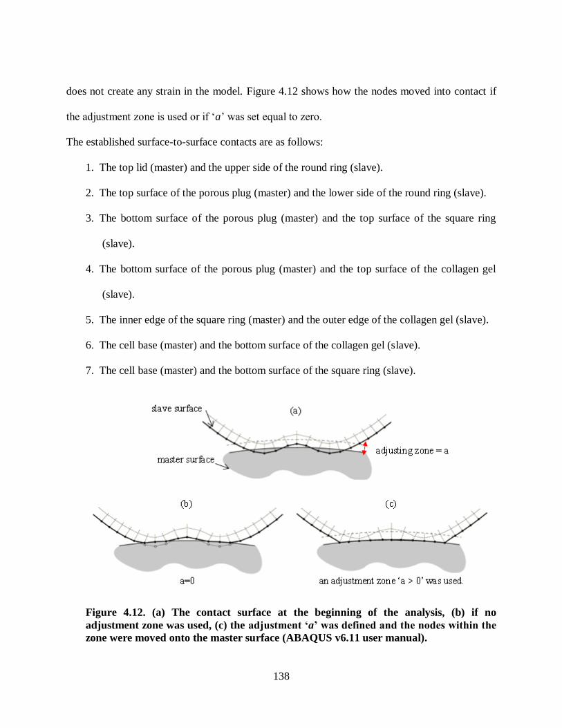
138

does not create any strain in the model. Figure 4.12 shows how the nodes moved into contact if

the adjustment zone is used or if „a‟ was set equal to zero.

The established surface-to-surface contacts are as follows:

1. The top lid (master) and the upper side of the round ring (slave).

2. The top surface of the porous plug (master) and the lower side of the round ring (slave).

3. The bottom surface of the porous plug (master) and the top surface of the square ring

(slave).

4. The bottom surface of the porous plug (master) and the top surface of the collagen gel

(slave).

5. The inner edge of the square ring (master) and the outer edge of the collagen gel (slave).

6. The cell base (master) and the bottom surface of the collagen gel (slave).

7. The cell base (master) and the bottom surface of the square ring (slave).

Figure 4.12. (a) The contact surface at the beginning of the analysis, (b) if no

adjustment zone was used, (c) the j s m n ‘a’ w s fin n h no s wi hin h

zone were moved onto the master surface (ABAQUS v6.11 user manual).

139

The meshes were matched between the contact surfaces at the beginning of the computational

analysis to obtain a better convergence rate and thus more accuracy (Figure 4.11).

A pore pressure degree of freedom existed on both sides of the contact interfaces, as the collagen

gel and the porous plug were defined as poroelastic materials. The contact surface between the

upper side of the collagen gel and the bottom surface of the porous plug should allow for the free

movement of fluid and a biphasi “jump ondition” should need to be satisfied (Hou et al. 1989):

0nqnvv sff , 4.6

where q is the fluid flow, f is the fluid phase volumetric fraction, sv and fv are the solid and

fluid phase fluid velocities, respectively, and n is the outward normal to the contact interface.

The fluid flowed in the direction normal to the contact interface and did not flow tangentially

along the surface (ABAQUS v6.11 neglected the tangential flow). The flow normal to the

interface was defined as follows (Federico et al. 2004, Pawaskar, Fisher and Jin 2010)

(ABAQUS v6.11 user manual):

BAcacross ppkq . 4.7

where acrossq was the fluid flow normal to the interface, Ap and Bp were pore pressures at points

on opposite sides of the interface (master and slave); and ck was the contact permeability with

units of Ns

mm3

.

A positive value of pressure gradient corresponded to fluid flow out from the master surface or

flow into the slave surface, while a negative pressure gradient represented that no flow could

exude from the master surface and the fluid from the slave surface flows into the master surface.

140

The contact permeability was set equal 1 Ns

mm3

and thus the fluid could flow freely between the

contact interfaces (Pawaskar et al. 2010, Federico et al. 2004).

The axial compression load was applied to the cell base at a constant rate of 1 N/s for 20

seconds. The collagen gel was compressed between the base and the permeable porous plug, and

was confined by the sides of the square ring and the base. Therefore, the deformation was

predominantly in the axial direction. The compressive stress in the gel increased due to

pressurization of the fluid phase. The solid matrix was compressed as the interstitial fluid was

forced out of the scaffold. The square ring, due to its greater stiffness, controlled the overall

strain of the collagen. The total displacement of the cell base was the sum of the deformations of

the square ring and round ring (Figure 4.13).

0

4

8

12

16

20

0 0.1 0.2 0.3 0.4 0.5 0.6 0.7 0.8

Forc

e [N

]

Displacement [mm]

Whole system including the gel

Base Round Ring Square Ring or Collagen

Figure 4.13. Model predictions of the force-displacement curve for the whole system

including the collagen gel under confined compression: ramp load with the rate of 1 N/s.

The distribution of axial strain demonstrated that the elements at the superficial layers of the

collagenous scaffold experienced higher peak strains and fluid velocities (Figure 4.14). Four

sample elements were selected in the axial direction to examine the effect of confined

141

compression under the applied ramp load. During the initial ramp phase the elements closer to

the plug experienced higher magnitudes of compression. For instance, the element at the top

under a 20 N compression load experienced 40 % compressive strain and a fluid velocity of 6

µm/s, whereas the mechanical stimuli for the middle or bottom elements were 3 % compressive

strain and a fluid velocity of 4105 µm/s (Figure 4.15, Figure 4.16).

Axial strain, collagenous scaffold

Symmetry line

t=20 s

Symmetry line

Fluid velocity [mm/s], collagenous scaffoldt=20 s

Figure 4.14. Distribution of axial strain (EE2) and fluid velocity (FLVEL, [mm/s]), within

the collagenous scaffold under 20 N axial compression load at t=20 s.

142

Figure 4.15. Change of fluid velocity over time within four sample elements of the

collagenous scaffold. The scaffold was loaded at a rate of 1 N/s. Four sample elements are

shown through the depth of the collagen (at the right).

Figure 4.16. Change of axial strain over time within four sample elements of the

collagenous scaffold The scaffold was loaded at a rate of 1 N/s. Four sample elements are

shown through the depth of the collagen (at the right).

The displacement of the rings and the cell base were compared in two models: (1) the

collagenous gel not included in the simulation (Figure 4.9); (2) the collagenous gel included in

the model (Figure 4.17). The total displacement was greater for the model without the gel

(Figure 4.17). The solid phase transferred a significant portion of the load to the interstitial fluid

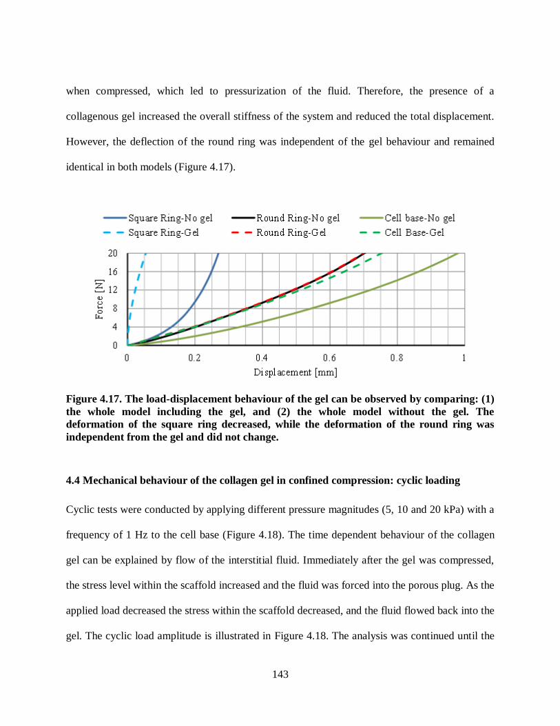
143

when compressed, which led to pressurization of the fluid. Therefore, the presence of a

collagenous gel increased the overall stiffness of the system and reduced the total displacement.

However, the deflection of the round ring was independent of the gel behaviour and remained

identical in both models (Figure 4.17).

Figure 4.17. The load-displacement behaviour of the gel can be observed by comparing: (1)

the whole model including the gel, and (2) the whole model without the gel. The

deformation of the square ring decreased, while the deformation of the round ring was

independent from the gel and did not change.

4.4 Mechanical behaviour of the collagen gel in confined compression: cyclic loading

Cyclic tests were conducted by applying different pressure magnitudes (5, 10 and 20 kPa) with a

frequency of 1 Hz to the cell base (Figure 4.18). The time dependent behaviour of the collagen

gel can be explained by flow of the interstitial fluid. Immediately after the gel was compressed,

the stress level within the scaffold increased and the fluid was forced into the porous plug. As the

applied load decreased the stress within the scaffold decreased, and the fluid flowed back into the

gel. The cyclic load amplitude is illustrated in Figure 4.18. The analysis was continued until the

144

tissue subsided to a steady state to explore the influence of mechanical loading on temporal and

spatial cellular responses in the Flexcell experiments with time in culture. The stress at the

equilibrium point represented the stress within the solid phase.

Figure 4.18. The amplitude of the applied cyclic axial compression loads. The pressure,

ranging from 5-20 [kPa], was applied to the cell base with a frequency of 1 Hz.

A 5 kPa (1 Hz) was applied at the bottom until the pore pressure subsided to a steady state (300

s) to mimic experimental investigations. Three sample elements were selected through the axial

depth of the gel: (1) top element at the top surface of the gel, (2) the middle element, and (3) the

bottom element at the bottom of the gel. The strain curve of the top sample element over the first

40 seconds is presented in Figure 4.19. The superficial layers experienced higher peak strains

and pore pressure compared to the deeper layers (Figure 4.20, Figure 4.21 and Figure 4.23). The

scaffold was strained non-uniformly due to a relatively quick compression. The superficial layers

experienced 3.3 % axial compressive strain, while an internal tension was generated at the deeper

layers. Although initially the magnitudes of strain, fluid velocity and the pore pressure were

higher at the superficial layers of the scaffold, after approximately 300 s the system reached an

equilibrium state. The nonhomogeneous distribution of the peak strain relaxed to an

145

approximately constant value of 1.6 % axial compression and 1.2 % octahedral shear strain

(Figure 4.20, Figure 4.21). The fluid velocity increased to 1.3 [µm/s] and at the equilibrium stage

had subsided to 0.2 µm/s (Figure 4.22). The fluid pore pressure at the equilibrium state went to

zero. Therefore, the pore pressure at peak loading represented the stress of 0.02 [MPa] in the

solid phase at the equilibrium state (Figure 4.23).

Figure 4.19. Model prediction for the axial strain during confined compression: cyclic

loading (P=5 kPa, 1 Hz). Compressive strain in top element under axial compression.

Figure 4.20. Prediction of axial strain at the peak loading in three selected sample elements

in the collagenous scaffold in confined compression under cyclic loading of P=5 kPa (1 Hz).

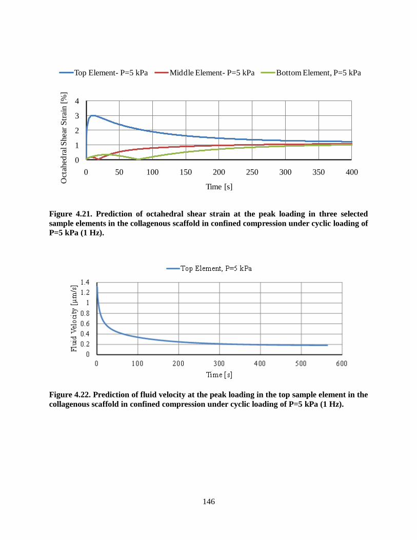
146

0

1

2

3

4

0 50 100 150 200 250 300 350 400

Oct

ahed

ral S

hea

r S

trai

n [

%]

Time [s]

Top Element- P=5 kPa Middle Element- P=5 kPa Bottom Element, P=5 kPa

Figure 4.21. Prediction of octahedral shear strain at the peak loading in three selected

sample elements in the collagenous scaffold in confined compression under cyclic loading of

P=5 kPa (1 Hz).

Figure 4.22. Prediction of fluid velocity at the peak loading in the top sample element in the

collagenous scaffold in confined compression under cyclic loading of P=5 kPa (1 Hz).

147

0

0.02

0.04

0.06

0.08

0 50 100 150 200 250 300 350 400 450pore

pre

ssure

[M

Pa]

Time [s]

Top Element, P=10 kPa Middle Element, P=10 kPa Bottom Element, P=10 kPa

Figure 4.23. Prediction of pore pressure at the peak loading in three selected sample

elements in the collagenous scaffold in confined compression under cyclic loading of P=5

kPa (1 Hz).

Three different pressure levels with the same loading rate (5, 10 and 20 kPa, 1 Hz) were applied

to the cell base to investigate the effect of load magnitude on the mechanical stimuli, temporally

and spatially. A longer time was required to reach a steady state and the strain value increased in

the collagen matrix with increased applied pressure (Figure 4.24). The predicted equilibrium

strains were 7.7, 3.4 and 1.6 % within the solid section (top sample element), when the cell base

was under 20, 10 and 5 kPa pressure, respectively.

The stress-strain response of the collagenous scaffold is shown for the 10 kPa (1 Hz) case

(Figure 4.25). As the gel was compressed, the solid matrix deformed and the interstitial fluid was

forced out of the gel, which led to an increase in the deformation of the collagen matrix and an

increase in fluid pressure. However, by decreasing the pressure to zero, the fluid flowed back

into the gel, which led to a decrease in the strain level within the solid phase. The time dependant

nature of the gel could be observed by the stress-strain curve during the loading and unloading

(hysteresis). The width of the ellipses in Figure 4.25 illustrates the energy loss due to viscous

148

dissipation and fluid exudation from the gel. The initial loading cycles were associated with a

stiffer response and greater energy loss.

Figure 4.24. Comparison of axial strains at the peak loading in the top sample element in

the collagenous scaffold in confined compression under different cyclic applied loads of

P=5, 10, 20 kPa (1 Hz).

Figure 4.25. The gel was subjected to 10 kPa pressure (1 Hz). The hysteresis of the stress-

strain curve shows the effects of the interstitial flow and viscous dissipation (the graph

shows the first 33 seconds of analysis).

149

The mechanical behaviour of the 1D FE model of the modified Flexcell system was validated

against experimental results (Figure 4.10) (Olesja Hazenbiller, M.Sc. student, University of

Calgary). The influence of mechanical loading on temporal and spatial cellular responses was

explored. The response of the collagen gel in confined compression under cyclic loads up to 20

kPa was evaluated. The magnitudes of axial strain, fluid velocity and pore pressure were

predicted at the peak loading in the top, middle and bottom sample elements. As the applied

pressure increased, the equilibrium strain, fluid velocity and pore pressure increased (Table 4.3).

This model provides a tool to understand the internal stress-strain response within the modified

Flexcell system for mechanobiological experiments with very soft gels.

Table 4.3. The predicted equilibrium strains, fluid velocities and pore pressure at the peak

loading in the top, middle and bottom sample elements.

Pressure [kPa] Axial strain [%] Fluid velocity [µm/s] Pore pressure [MPa]

Top sample element

5 (1 Hz) 1.6 0.18 0.01

10 (1 Hz) 3.4 0.43 0.02

20 (1 Hz) 7.7 1.06 0.05

Middle sample element

5 (1 Hz) 1.4 0.001 0.01

10 (1 Hz) 3.1 0.010 0.02

20 (1 Hz) 6.3 0.040 0.05

Bottom sample element

5 (1 Hz) 1.3 0.00007 0.01

10 (1 Hz) 3.0 0.00070 0.02

20 (1 Hz) 5.8 0.00200 0.05

4.5 Prediction of tissue differentiation in confined compression

The aim of this study was to investigate the effect of mechanical loading on a stem cell seeded

collagenous scaffold under confined compression. FE modelling and mechanoregulatory

algorithms were used to explore the influence of mechanical loading on temporal and spatial

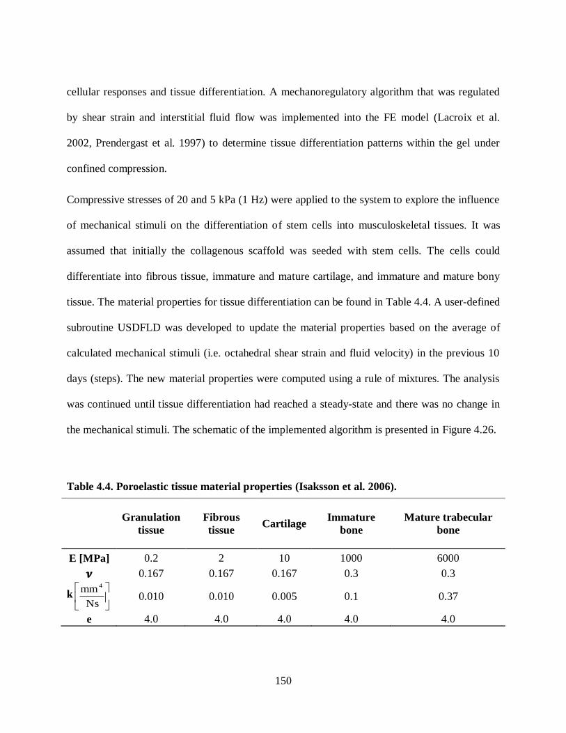
150

cellular responses and tissue differentiation. A mechanoregulatory algorithm that was regulated

by shear strain and interstitial fluid flow was implemented into the FE model (Lacroix et al.

2002, Prendergast et al. 1997) to determine tissue differentiation patterns within the gel under

confined compression.

Compressive stresses of 20 and 5 kPa (1 Hz) were applied to the system to explore the influence

of mechanical stimuli on the differentiation of stem cells into musculoskeletal tissues. It was

assumed that initially the collagenous scaffold was seeded with stem cells. The cells could

differentiate into fibrous tissue, immature and mature cartilage, and immature and mature bony

tissue. The material properties for tissue differentiation can be found in Table 4.4. A user-defined

subroutine USDFLD was developed to update the material properties based on the average of

calculated mechanical stimuli (i.e. octahedral shear strain and fluid velocity) in the previous 10

days (steps). The new material properties were computed using a rule of mixtures. The analysis

was continued until tissue differentiation had reached a steady-state and there was no change in

the mechanical stimuli. The schematic of the implemented algorithm is presented in Figure 4.26.

Table 4.4. Poroelastic tissue material properties (Isaksson et al. 2006).

Granulation

tissue

Fibrous

tissue Cartilage

Immature

bone

Mature trabecular

bone

E [MPa] 0.2 2 10 1000 6000

0.167 0.167 0.167 0.3 0.3

k

Ns

mm 4

0.010 0.010 0.005 0.1 0.37

e 4.0 4.0 4.0 4.0 4.0

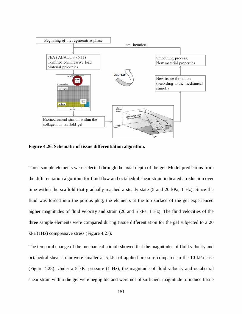
151

Figure 4.26. Schematic of tissue differentiation algorithm.

Three sample elements were selected through the axial depth of the gel. Model predictions from

the differentiation algorithm for fluid flow and octahedral shear strain indicated a reduction over

time within the scaffold that gradually reached a steady state (5 and 20 kPa, 1 Hz). Since the

fluid was forced into the porous plug, the elements at the top surface of the gel experienced

higher magnitudes of fluid velocity and strain (20 and 5 kPa, 1 Hz). The fluid velocities of the

three sample elements were compared during tissue differentiation for the gel subjected to a 20

kPa (1Hz) compressive stress (Figure 4.27).

The temporal change of the mechanical stimuli showed that the magnitudes of fluid velocity and

octahedral shear strain were smaller at 5 kPa of applied pressure compared to the 10 kPa case

(Figure 4.28). Under a 5 kPa pressure (1 Hz), the magnitude of fluid velocity and octahedral

shear strain within the gel were negligible and were not of sufficient magnitude to induce tissue

152

differentiation. According to the biphasic algorithm small magnitudes of strain and fluid velocity

lead to bony tissue formation (Lacroix et al. 2002). When the scaffold was subjected to a 5 kPa

pressure the mechanical stimuli were very small, and thus the algorithm predicted cartilage and

bone tissue formation. The predicted sequence of tissue differentiation in the gel subjected to a 5

kPa pressure did not occur in the same pattern observed in vitro (not shown), which shows that

the mechanoregulatory algorithm could not properly model the actual tissue differentiation

process.

Figure 4.27. Prediction of fluid velocity at the peak loading in three sample elements in the

collagenous scaffold during tissue differentiation (P = 20 kPa, 1 Hz).

When the system was subjected to a 20 kPa compressive stress (1 Hz) tissue differentiation was

promoted in the zones closer to the loading but the superficial layers had delayed tissue

differentiation. The fibrous tissue differentiation initiated from the bottom regions, followed by

differentiation into a cartilaginous tissue, which then spread throughout the scaffold gradually.

At day 6 (step 6), small amounts of undifferentiated tissue still existed at the top surface of the

153

gel (Figure 4.29b). In the superficial regions the higher values of mechanical stimuli resulted in

increased fluid flow, which delayed the differentiation process into cartilaginous tissues for the

20 kPa load case (Figure 4.28, Figure 4.29b).

Figure 4.28. Mechanical stimuli in a sample element at the superficial layer for a 5 kPa and

a 20 kPa (1 Hz) compressive pressure applied to the system.

Gene expression analysis within the stem cell seeded collagenous scaffold from our experimental

studies indicated that the 3D collagen1 gels at day 15 had promoted chondrogenesis (Figure 4.29,

Figure 4.30) (Olesja Hazenbiller, M.Sc. student, University of Calgary). In agreement with the

experimental results the gel became stiffer by differentiating into cartilaginous tissues as

predicted by the finite element analysis (Figure 4.29a, Figure 4.29b, Figure 4.30).

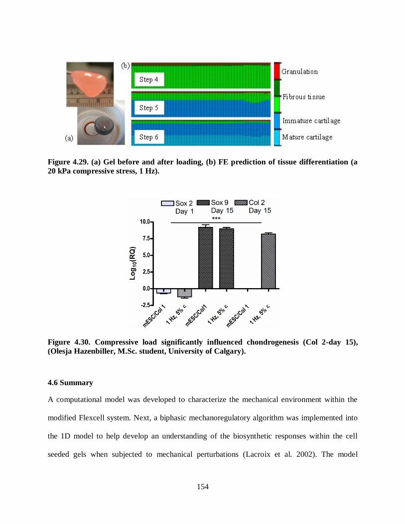
154

Figure 4.29. (a) Gel before and after loading, (b) FE prediction of tissue differentiation (a

20 kPa compressive stress, 1 Hz).

Figure 4.30. Compressive load significantly influenced chondrogenesis (Col 2-day 15),

(Olesja Hazenbiller, M.Sc. student, University of Calgary).

4.6 Summary

A computational model was developed to characterize the mechanical environment within the

modified Flexcell system. Next, a biphasic mechanoregulatory algorithm was implemented into

the 1D model to help develop an understanding of the biosynthetic responses within the cell

seeded gels when subjected to mechanical perturbations (Lacroix et al. 2002). The model

155

predictions suggested that loading the stem cell-seeded soft gel led to differentiation of stem cells

into cartilaginous tissue. Hence, the mechanical stimuli provided a suitable environment for cell

biosynthesis and differentiation. Both empirical and computational data suggest that mechanical

stimulation of the scaffold may be an effective way to initiate differentiation pathways prior to

implantation for tissue engineering applications. The computational and experimental studies

(e.g. gene expression, µCT, mechanical testing and the mineralization patterns) will be used

simultaneously in future studies to further develop mechanoregulatory models with a more

robust quantitative base.

156

Chapter Five: Tissue Differentiation in a Burr-hole Fracture Model in a Murine Tibia

This chapter presents a computational analysis of tissue differentiation within a burr-hole

fracture model of a murine tibia. A mechanoregulatory algorithm is implemented in a finite

element model of the in-vivo burr-hole fracture model developed by Taiani et al. (2010). The

tissue differentiation patterns to predict bone formation within the fracture are investigated for a

number of variables. An introduction to the software used to develop the finite element mesh is

first given to understand the required stages for the FE model regeneration and volumetric

meshing. Then, the steps to generate the FE models of the intact murine tibia are presented. Next,

the mechanical behaviour of the reconstructed model was validated against a previous

experimental-numerical study (Stadelmann et al. 2009). Subsequently, the development of the

burr-hole fracture model in the murine tibia are outlined. Finally, the biphasic

mechanoregulatory algorithm was implemented into the developed model to predict tissue

differentiation in the burr-hole model (Isaksson et al. 2006, Prendergast et al. 1997). The burr-

hole model was then filled with a stem cell seeded soft collagenous scaffold and tissue

differentiation was predicted for a variety of case studies:

1. tibia was subjected to axial compression loads ( 2, 1 and 0.5 N, 1 Hz),

2. different rate of cell diffusion (0.025 and 0.01 s

mm 2

),

3. different axial positions of the fracture (4.95, 3.13 and 2.55 mm),

4. different cell origins,

5. osteoporotic bone with poor mechanical behaviour, and

6. the tibia was also subjected to bending load (0.02, 0.04 Nm).

The overview of this chapter and computational investigations conducted is shown in Figure 5.1.

157

Reconstruction of a 3D murine tibia using

µCT images.

Mechanoregulatory algorithm.

Loading

conditions. Location of

the burr-hole.

Rate of

diffusion.

Verification against a previous experimental

study (Stadelmann et al., 2009).

Osteoporotic

bone.

Figure 5.1. Overview of this chapter.

5.1 Introduction

Micro computed tomography (µCT) is known as an imaging technique for medical purposes in a

minimally invasive way. Recently, this technique has been used to create precise FE models

from complex geometries (Silva, Brodt and Hucker 2005, Stadelmann et al. 2009). A three-

dimensional finite element model (3D FEM) of a murine tibia structure was recovered from

(µCT) scans and were meshed, using Simpleware v3.5.3 image processing software (Simpleware

Ltd., Exeter, UK). This software consists of three modules:

(1) ScanIP is the core image-processing platform. Medical file formats, such as CT, µCT,

and magnetic resonance imaging (MRI) data can be imported into the software for

processing and manipulation.

(2) ScanFE converts the segmented 3D images into volumetric or surface models. Mesh

generation is performed within this module for a variety of commercial FE platforms.

158

(3) ScanCADcan be used to modify models with Boolean operations on masks of the multi-

part models to add parts or create layers (e.g. union, subtraction, invertion and

intersection).

5.2 Reconstruction of a murine tibia

In this study, the FE reconstruction of an intact murine tibia was performed in three sequential

stages explained in the following sections.

5.2.1 Importing and preparing the data (ScanIP module)

The right tibia from a female CD1 mouse (8 weeks old, the skin and muscle were cleaned) was

scanned at a 7 µm resolution using a SCANCO Medical µCT 35 at fMcCaig Institute (University

of Calgary). Full-length scans were obtained consisting of 2883 slices. Tagged image file format

(TIFF) data were created with 0.007 mm interval and imported into the ScanIP module. The

histogram, i.e. a graph showing the number of pixels at different intensity values, was computed

to find the frequency of the greyscale values for the various tissues. The histogram provided

information about the threshold values and noise reduction of the images. The memory required

for image analysis was estimated at 1900 Mb. To reduce the memory requirement, the empty

space around the object was cropped. The data were rescaled by assigning the pixel spacing of

0.03 mm in all directions using linear interpolation. Moreover, the resolution of the datasets was

down-sampled (i.e. increase the pixel spacing) to make the segmentation step faster and easier.

These steps reduced memory usage to a more manageable 97 Mb.

5.2.2 Image processing (ScanIP module)

When the data was imported into the ScanIP module, some noise (unnecessary points around the

object) was detected. The noise could result from the heterogeneous x-ray emission or the

inappropriate position of sample holder with respect to the x-ray source (e.g. the sample holder

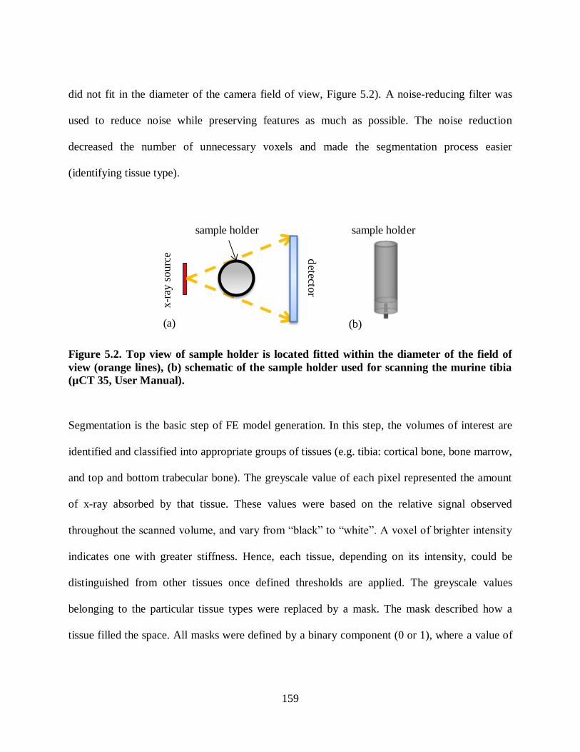
159

did not fit in the diameter of the camera field of view, Figure 5.2). A noise-reducing filter was

used to reduce noise while preserving features as much as possible. The noise reduction

decreased the number of unnecessary voxels and made the segmentation process easier

(identifying tissue type).

sample holder

detecto

r

x-r

ay s

ourc

e

sample holder

(a) (b)

Figure 5.2. Top view of sample holder is located fitted within the diameter of the field of

view (orange lines), (b) schematic of the sample holder used for scanning the murine tibia

(µCT 35, User Manual).

Segmentation is the basic step of FE model generation. In this step, the volumes of interest are

identified and classified into appropriate groups of tissues (e.g. tibia: cortical bone, bone marrow,

and top and bottom trabecular bone). The greyscale value of each pixel represented the amount

of x-ray absorbed by that tissue. These values were based on the relative signal observed

throughout the s anned volume, and vary from “ la k” to “white”. A voxel of righter intensity

indicates one with greater stiffness. Hence, each tissue, depending on its intensity, could be

distinguished from other tissues once defined thresholds are applied. The greyscale values

belonging to the particular tissue types were replaced by a mask. The mask described how a

tissue filled the space. All masks were defined by a binary component (0 or 1), where a value of

160

zero meant that the pixel did not belong to the tissue whereas a value of one meant that the pixel

belonged to the tissue.

In our case, four masks were needed: cortical bone, bone marrow, and proximal and distal

trabecular bone. To render our sample in three dimensions, a threshold-based method was used

to segment the raw data. Each tissue was distinguished by the lower and upper threshold bounds

depending on the range of the tissue greyscale values. In ScanIP, the greyscale values were

represented by integers in the range of 0-255. The appropriate threshold level was determined for

each tissue. The cortical bone could be distinguished visually from the trabecular bone (Figure

5.3). Since the cortical bone was stiffer compared to the trabecular bone, the upper threshold

bound of 255 was used for the cortical. In order to find the optimum lower threshold parameter

for the cortical bone, different masks were created using different lower and upper threshold

bounds: [50, 255], [100, 255], [200, 255] and [225, 255]. In the first three bounds, the trabecular

bone was also included in the mask. Hence, the lower threshold bound for cortical bone was

higher than 200. Different bounds were tested and finally the lower and upper threshold bounds

of 202 and 255 were selected for cortical bone. The upper bound for trabecular bone was set 201

and a similar set of steps were conducted to distinguish the lower threshold bound for trabecular

bone ([1, 201], [50, 201], [100, 201], [150,201]). Values less than 190 were determined to

represent the bone marrow. Therefore, 190 and 201 for trabecular bone, and the values lower

than 190 were used to construct the bone marrow.

161

Figure 5.3. Cortical and trabecular bone could be visually distinguished in the µCT cross-

sectional view of a murine tibia.

The threshold-based method was used to create the mask for the cortical bone. Erroneous holes

and isolated small areas may appear after segmentation due to noise absorption in the scanning

stage. First, the morphological close filter was used to add connectivity to the cortical mask, and

then the cavity fill filter was performed to fill the remaining small holes in the cortical mask. The

avity fill filter filled “internal” holes while preserving the outer boundaries of the marrow

cavity. Thereafter, the island removal filtration was carried out to have a continuum mask and

get rid of the redundant islands (detached segmented pixels in the cortical mask). To facilitate the

meshing process minor editing was necessary to smooth out the sharp edges near the ends of the

tibia. The sharp edges at the ends of the tibia were erased using the paint segmentation tool.

Finally, the re ursive Gaussian filter with the value of σ = 0.045 mm (1.5 times the spacing) was

performed to increase the smoothness of the segmented cortical surfaces (Figure 5.4). The larger

values of σ resulted in smoother surfaces, and it was suggested by the software to use the values

of 1 times to 3 times the spacing of the image data (0.03 mm) for smoothing the model.

162

(a)

(b)

Figure 5.4. Bone geometry before and after applying the recursive Gaussian filter.

After the cortical mask had been created, the trabecular mask was segmented using again the

threshold-based method (lower and upper threshold values, [190, 201]). To create a continuous

mask, initially the morphological close filter was used to merge fine structures of the trabecular

bone. Next, the cavity fill filter was internal holes of the trabecular mask, which are neither

connected to the cortical bone or bone marrow. However, due to the spongy structure of the

trabecular bone, the spaces between the trabeculae were very large and only some of them were

filled using the cavity fill filter. Then, the floodfill filter was used to fill the remaining gaps

between the trabeculae. In case of an overlap (between the cortical and trabecular mask), the

Boolean subtraction was performed and the trabecular mask subtracted from the cortical mask. A

similar set of steps was used to establish the mask for the bone marrow. The created masks are

shown in Figure 5.5. The masks in different locations of the tibia can be seen in Figure 5.5, with

the cortical mask shown in red, trabecular masks in blue and marrow mask in yellow.

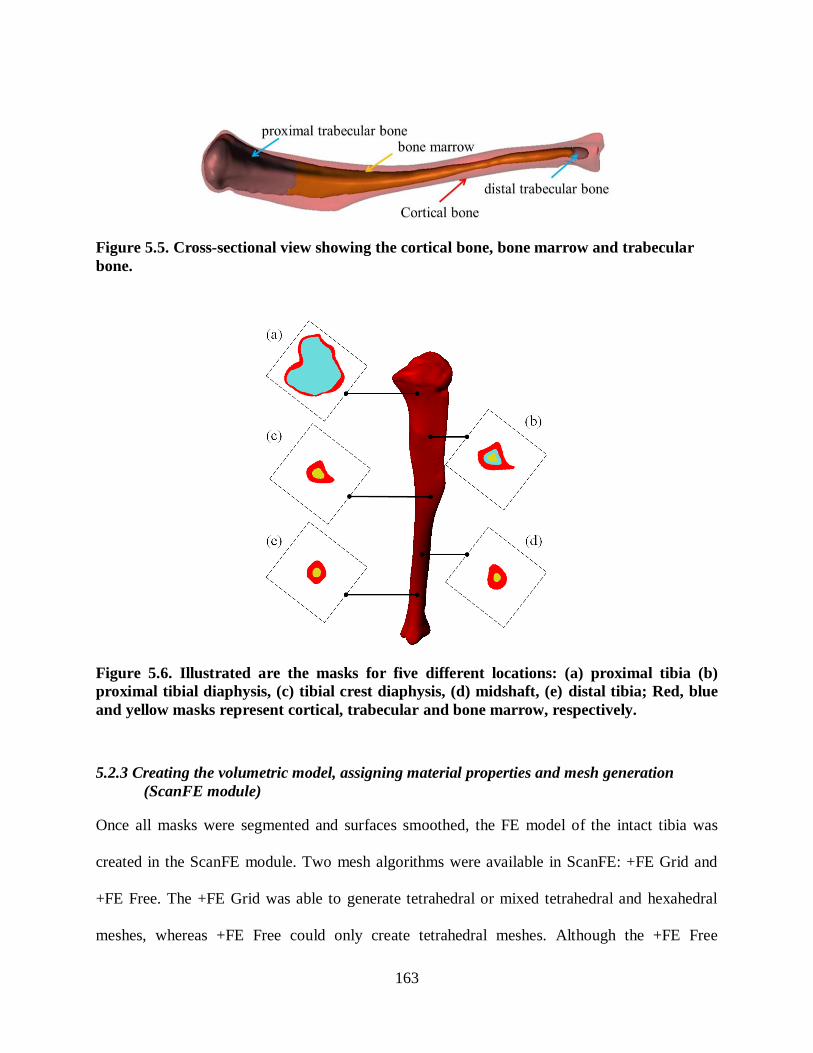
163

Figure 5.5. Cross-sectional view showing the cortical bone, bone marrow and trabecular

bone.

Figure 5.6. Illustrated are the masks for five different locations: (a) proximal tibia (b)

proximal tibial diaphysis, (c) tibial crest diaphysis, (d) midshaft, (e) distal tibia; Red, blue

and yellow masks represent cortical, trabecular and bone marrow, respectively.

5.2.3 Creating the volumetric model, assigning material properties and mesh generation

(ScanFE module)

Once all masks were segmented and surfaces smoothed, the FE model of the intact tibia was

created in the ScanFE module. Two mesh algorithms were available in ScanFE: +FE Grid and

+FE Free. The +FE Grid was able to generate tetrahedral or mixed tetrahedral and hexahedral

meshes, whereas +FE Free could only create tetrahedral meshes. Although the +FE Free

164

approach had slower mesh generation, it had more flexibility in the element creation process and

offered more control over the element size and mesh density. The minimum and maximum edge

length, the target maximum error and the surface change rate could be defined in the advanced

parameter settings. The target maximum error is the distance that the remeshed surface can move

from the original mesh. Surface change rate defines how fast the size of the elements can alter

during meshing; higher rates reduce the mesh quality.

In the present study, the +FE Free meshing algorithm was applied to have more control over the

element size, number and quality. The maximum and minimum target edge length (0.4 and 0.6

mm) and other options were defined in the advanced parameter settings. Three mesh densities

were generated for mesh convergence and sensitivity analysis. The selection of the element size

was made on the basis of a convergence study.

The material properties, e.g. the Young‟s modulus and oisson‟s ratio, were defined in the

material tab of the ScanFE module. Three material type options were available: placeholder,

homogeneous and greyscale based. The material properties could be defined later in the FE

software by choosing the placeholder option. The homogeneous option defined the material

model as linear elasti . A Young‟s modulus and oisson‟s ratio of 2.0 [MPa] and 0.167,

respectively, were specified for the bone marrow (Isaksson et al. 2006). The greyscale based

option automated the material properties for each tissue based on the image density and was used

for the cortical bone and trabecular bone within the present study. The greyscale values were

mapped to a mass density, and the mass density was mapped to a Young‟s modulus and

oisson‟s ratio. The mapping fun tion was assumed to be linear. The greyscale values of each

voxel were mapped to the mass density ( ) using the following equation:

GSβαρ 5.1

165

where GS was the element greyscale value and α and β were the mapping oeffi ients. Young‟s

modulus (E) and oisson‟s ratio (ν) were computed from the mass density for each element

(Equations 5.2, 5.3).

cbρaρE 5.2

dρν 5.3

where a, b and c were defined based on the published equations by Rho et al. (1995) for a

longitudinal compressed human tibia bone (Table 5.1) (Rho et al. 1995, Stadelmann et al. 2009).

The constants (a, b, c and d) defined the mapping function. The range of greyscale based

Young‟s modulus values that were assigned to the masks are shown in Table 5.2. The

Simpleware software uses a formulation derived for humans (Rho et al, 1995). Since there was

no available data that related the murine density to its Young‟s modulus, equation (5.2) was

used. However, experimental studies should be performed in future to scale the formula for the

murine tibia. After assigning the meshing parameters and defining the material properties,

volume meshes were generated in the ScanFE module. Figure 5.7 presents anterior, posterior,

medial and lateral views of the meshed murine tibia. An input file was then generated and

imported into ABAQUS v6.11. Figure 5.8 summarizes the required steps from greyscale data to

generation of the volumetric mesh.

Table 5.1. The relationship between the mechanical properties and mass density (Rho et al.

1995).

Dependent variable Tibial cortical bone Tibial trabecular bone

Density [3mkg ] GS0.916114ρ GS0.916114ρ

Yo ng’s mo l s [MPa] 13ρ-3842E 5.54ρ-326E

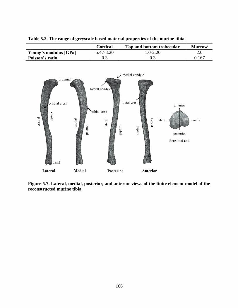
166

Table 5.2. The range of greyscale based material properties of the murine tibia.

Cortical Top and bottom trabecular Marrow

Yo ng’s mo l s [GP ] 5.47-8.20 1.0-2.20 2.0

Poisson’s io 0.3 0.3 0.167

Figure 5.7. Lateral, medial, posterior, and anterior views of the finite element model of the

reconstructed murine tibia.

167

Figure 5.8. (a) Volume image, (b) greyscale data, (c) segmented mask, (d) isolated

segmented mask, (e) smoothed mask (recursive Gaussian filter), (f) mesh generation of the

extracted volume.

5.2.4 Convergence study

A convergence test was carried out to ensure the selected number of elements was sufficient to

predict the mechanical behaviour of the tibia. A linear elastic material model was applied to the

regenerated model. Three meshes with increasing density (74665, 84580 and 96563 elements)

were created to asses mesh convergence. The higher density meshes were obtained using an

minimum element size of 0.4 mm and a maximum element size of 0.6 mm. The meshing with the

medium density was composed of elements in the range of 0.25 to 0.4 mm, and the highest

density meshes were meshed using the element size in the range of 0.2 to 0.4 mm.

Both linear and nonlinear geometric models were simulated to evaluate their effects on the

results. The tissues were composed of 10-node quadratic tetrahedron elements (C3D10). The

convergence study was performed for an applied axial compressive load of 2 N to the proximal

point of the tibia. All the nodes at the distal end were restricted in all directions. To evaluate the

168

mesh sensitivity, the maximum axial displacement in the model, and the summation of the axial

reaction forces at the distal nodes were considered for convergence. The increase in the element

number resulted in less than 0.1 % difference for the maximum displacement, and 0.2 % for the

axial reaction force at the distal end (Table 5.3). Hence, it was concluded that 74665 elements

were adequate for an accurate estimation of the mechanical behaviour within the model.

Table 5.3. Convergence study for three mesh densities.

Total element number 74665 84580 96563

Axial reaction force [N] 1.8439 1.8510 1.8472

Max. displacement [mm] 0.7688 0.7683 0.7691

Error in the axial reaction force [%] 0.177 0.208 -

Error in the max. displacement [%] 0.039 0.104 -

5.3 Verification of the generated FE model of the intact tibia

The mechanical behaviour of the reconstructed tibia was verified against a previously published

numerical-experimental study (Stadelmann et al. 2009). To match the experimental study, the

distal zone of the tibia was completely fixed. Axial compression loads were applied to the

proximal end increasing from zero to 10 N. The force-strain behaviour in a murine tibia was

determined at three different locations (proximal, midshaft and distal tibia) (Figure 5.9). In

Figure 5.9, the flat surface with the widest area at the proximal region represented the proximal

tibia (zone1), the region between the tibial crest and fibula junction was defined as the midshaft

tibia (zone 2), and the region between the fibula junction to the end of the tibia was defined as

the distal tibia (zone 3). The tissues were considered linear elastic and were meshed with 10-

node quadratic tetrahedron elements (C3D10). The material properties used are shown in Table

169

5.2. Principal strain values were estimated numerically at the three different regions of the tibia

(zone 1, zone 2 and zone 3) for comparison with strain-gauge measurements (Stadelmann et al.

2009). Figure 5.10 shows that the strain magnitudes were in good agreement with the

experimental values (maximum 10 % deviation) of Stadelmann et al. (2009). The maximum,

minimum and medium principal strains are shown when the bone was subjected to a 10 N axial

compression load (Figure 5.11).

Figure 5.9. Three zones that were compared: zone 1 (proximal tibia), zone 2 (tibial crest),

zone 3 (distal tibia).

(a) (b)

Figure 5.10. Force-strain relations measured by (a) Stadelmann et al. (2009), and (b)

predicted in the present study.

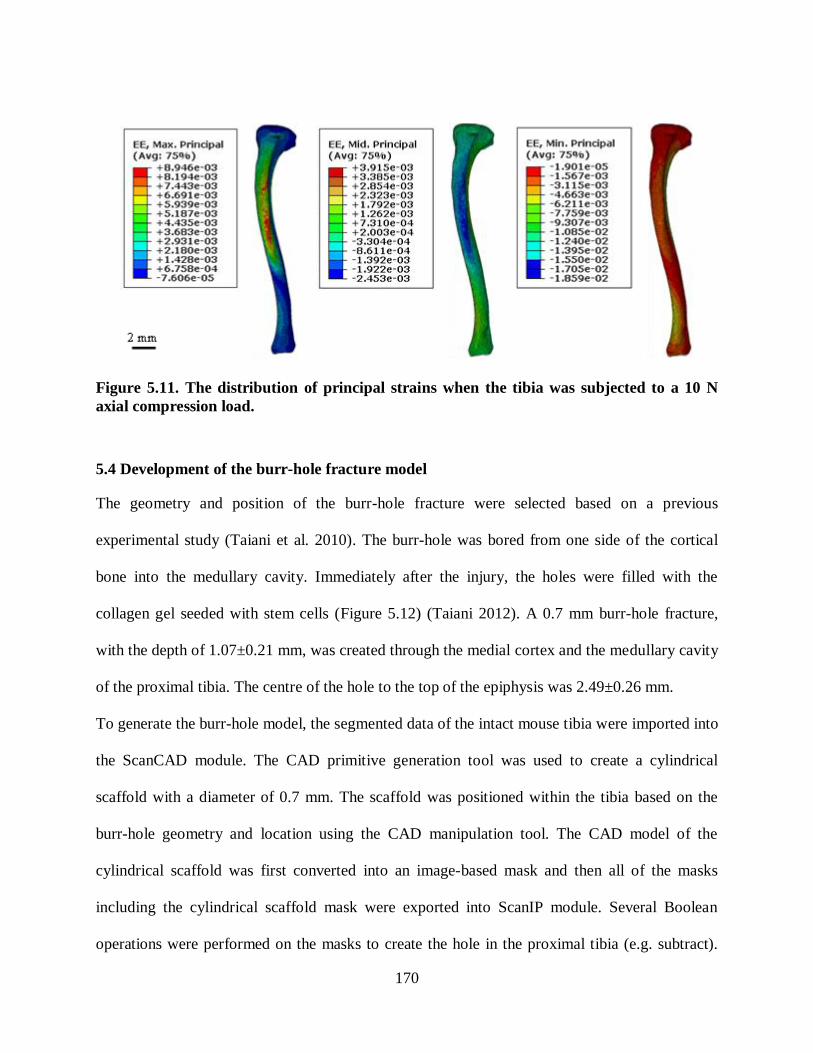
170

Figure 5.11. The distribution of principal strains when the tibia was subjected to a 10 N

axial compression load.

5.4 Development of the burr-hole fracture model

The geometry and position of the burr-hole fracture were selected based on a previous

experimental study (Taiani et al. 2010). The burr-hole was bored from one side of the cortical

bone into the medullary cavity. Immediately after the injury, the holes were filled with the

collagen gel seeded with stem cells (Figure 5.12) (Taiani 2012). A 0.7 mm burr-hole fracture,

with the depth of 1.07±0.21 mm, was created through the medial cortex and the medullary cavity

of the proximal tibia. The centre of the hole to the top of the epiphysis was 2.49±0.26 mm.

To generate the burr-hole model, the segmented data of the intact mouse tibia were imported into

the ScanCAD module. The CAD primitive generation tool was used to create a cylindrical

scaffold with a diameter of 0.7 mm. The scaffold was positioned within the tibia based on the

burr-hole geometry and location using the CAD manipulation tool. The CAD model of the

cylindrical scaffold was first converted into an image-based mask and then all of the masks

including the cylindrical scaffold mask were exported into ScanIP module. Several Boolean

operations were performed on the masks to create the hole in the proximal tibia (e.g. subtract).

171

The multipart volumetric model was meshed in ScanFE module using the +FE Free meshing

algorithm. The model was meshed using different target edge lengths, and finally the best mesh

was selected based on the information obtained from the element qualities: (1) the mesh statistics

in Simpleware, and (2) performing a mesh sensitivity analysis. In Simpleware, the mesh statistics

was in the log toolbox and gave a summary of the number of elements, nodes, average and the

worst element qualities. The maximum and minimum lengths of the elements for the cortical,

bone marrow and trabecular bone masks were set as 0.4 and 0.6 mm. To ensure accurate

mechanical behaviour within the fracture site (e.g. strain and fluid velocity) a finer discretization

was used to mesh the region of interest (scaffold). An element size of 0.2 mm was set in the

mesh refinement volume tool for the scaffold. After setting the mesh parameters and material

properties, the model was meshed with the total of 79790 elements and the input file was

generated and imported into ABAQUS v6.11 for computational analysis. The stages required to

generate the volumetric mesh are summarized in Table 5.4, and Figure 5.13 and 5.14.

Table 5.4. Elements numbers for different parts of the fracture model.

Cortical Proximal

trabecular

Distal

trabecular Scaffold Marrow Total

Number of

elements 43911 16462 1341 1890 16186 79790

172

Figure 5.12. Location of the burr-hole in the medial aspect of the tibia: (a) FE model, (b)

experimental fracture model (Taiani 2012). A section through the long axis of the burr-

hole: (c) FE model, (d) experimental fracture model (Taiani 2012). A section through the

frontal plane of the fractured tibia: (e) FE model, (f) experimental fracture model (Taiani

2012).

173

µCTImage processing tool (ScanIP):

segmentation of the intact tibia.

CAD integration module (ScanCAD):

creating the scaffold.

converting the CAD model into mask.

creating hole using Boolean operations.

Mesh generation module (ScanFE):

creating the FE model.

the volumetric mesh generation.

Export to ScanIP

Export the meshed model

(input file) to

FE model ABAQUS

Figure 5.13. Workflow diagram outlining the required functions to reconstruct the 3D FE

burr-hole model.

Figure 5.14. Overview of the processes used to create the burr-hole model.

5.4.1 Selection of the decay length model

Saint-Venant‟s prin iple states that the fixed boundaries only have an effect on the stress-strain

distribution within nearby regions which are relatively far away from the indenter. The linear

elastic model of the intact full-length tibia was compared to three different decay length models.

To create the decay length models sections were created in the following regions: (1) the

proximal tibia, (2) the tibial crest, and (3) the distal tibia (Figure 5.15). The models were

subjected to a 10 N axial compression load at the proximal end while the distal end was

174

completely fixed in all models. The distributions of stress and strain in the models were

compared to the full-length model. According to the results the tibial crest model was the one

that had the closest stress-strain distribution to the full-length tibia.

Figure 5.15. The decay length models were subjected to a 10 N load to select the one that

had the closest mechanical environment compared to the full-length model. The red arrow

shows where the load was applied.

The stress-strain distributions within the fractured models of the tibial crest and the full-length

model were also compared. The fractured tibiae were subjected to an axial compression load 10

N at the proximal end while the bottom end was totally fixed. The mechanical environments

175

were also similar in the burr-hole models (Figure 5.16, 5.17, 5.18), in particular in the region of

interest around the burr-hole (Figure 5.19, Figure 5.20).

Figure 5.16. Distribution of von Mises stress: (a) full-length model, (b) decay length model

(tibial crest, medial view).

176


(tibial crest, medial view).

177


(tibial crest, lateral view).

Figure 5.19 Distribution of von Mises stress within the scaffold: (a) full-length model, (b)

decay length model (tibial crest, medial view).

178

Figure 5.20 Distribution of principal strains within the scaffold: (a) full-length model, (b)

decay length model (tibial crest, medial view).

5.5 Tissue differentiation predictions within the burr-hole fracture

Several parametric studies were performed with the FE model of the fractured tibia to investigate

the effect of different loading regimes (axial compression, bending), rate of cell diffusion, origin

of the progenitor cells, position of the burr-hole fracture and bone quality (osteoporotic bone)

(Table 5.5).

In the current study, the loads (0.5-2.5 N) were selected based on the previous in vivo studies

(0.5-13 N), (Stadelmann et al. 2009, Zhang and Yokota 2011, Gardner et al. 2006, De Souza et

al. 2005). The peak force acting on the tibia during normal walking was determined to be 1.2 N

(Prasad et al. 2010). In another study, the peak strains at the tibial midshaft were reported for

normal walking (200-300 µƐ) and jumping (400-600 µƐ), (De Souza et al. 2005). According to

the study by Stadelmann et al. the loads between ~1.2-2.1 N and ~2.8-4.2 N produced strains of

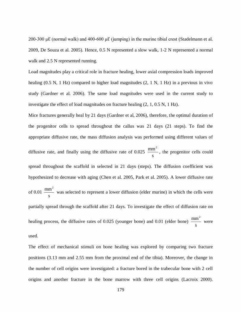
179

200-300 µƐ (normal walk) and 400-600 µƐ (jumping) in the murine ti ial rest (Stadelmann et al.

2009, De Souza et al. 2005). Hence, 0.5 N represented a slow walk, 1-2 N represented a normal

walk and 2.5 N represented running.

Load magnitudes play a critical role in fracture healing, lower axial compression loads improved

healing (0.5 N, 1 Hz) compared to higher load magnitudes (2, 1 N, 1 Hz) in a previous in vivo

study (Gardner et al. 2006). The same load magnitudes were used in the current study to

investigate the effect of load magnitudes on fracture healing (2, 1, 0.5 N, 1 Hz).

Mice fractures generally heal by 21 days (Gardner et al, 2006), therefore, the optimal duration of

the progenitor cells to spread throughout the callus was 21 days (21 steps). To find the

appropriate diffusive rate, the mass diffusion analysis was performed using different values of

diffusive rate, and finally using the diffusive rate of 0.025 s

mm 2

, the progenitor cells could

spread throughout the scaffold in selected in 21 days (steps). The diffusion coefficient was

hypothesized to decrease with aging (Chen et al. 2005, Park et al. 2005). A lower diffusive rate

of 0.01 s

mm2

was selected to represent a lower diffusion (elder murine) in which the cells were

partially spread through the scaffold after 21 days. To investigate the effect of diffusion rate on

healing process, the diffusive rates of 0.025 (younger bone) and 0.01 (elder bone) s

mm2

were

used.

The effect of mechanical stimuli on bone healing was explored by comparing two fracture

positions (3.13 mm and 2.55 mm from the proximal end of the tibia). Moreover, the change in

the number of cell origins were investigated: a fracture bored in the trabecular bone with 2 cell

origins and another fracture in the bone marrow with three cell origins (Lacroix 2000).

180

Furthermore, the osteoporotic bones are difficult to heal due to reduced mechanical properties

(Macdonald et al. 2011, Sharir et al. 2008). Osteoporotic bones were reported to have less

stiffness, Young‟s modulus and higher void ratio and permeability compared to the normal bones

(Li and Aspden 1997a, McDonnell et al. 2007, Sun et al. 2008). To investigate the effect of

reduced mechanical properties, a model of an osteoporotic murine tibia was used and its healing

rate compared to a normal bone. Moreover, bending load was reported an effective mean to

enhance bone formation in a murine tibia (Zhang et al. 2006). Hence, lateral loading were given

to the proximal end of the tibia to stimulate tissue differentiation (0.04, 0.02 Nm).

Table 5.5. Summary of the variables for the parametric studies.

Parametric studies Load

Diffusivity

[s

mm2

]

Number of

cell origins

Distance

[mm]

Axial compression 0.5, 1, 2 N 0.025 2 2.55

Cell diffusion rate 1 N 0.01, 0.025 2 2.55

Fracture

position

Trabecular

bone 1 N 0.025 2

2.55

3.13

Trabecular

bone and

bone marrow

2.5 N 0.025 2 2.55

3 4.95

Osteoporotic bone 2.5 N 0.025 2 2.55

Normal bone

Bending 0.02, 0.04

Nm 0.025 2 2.55

For all of the models, a stem cell seeded collagenous scaffold was initially implanted into the

gap. The cortical bone, bone marrow and trabecular bone tissues were defined as poroelastic

materials using 10-node modified quadratic tetrahedron pore pressure elements (C3D10MP). The

modified element used, had three additional displacement variables and one additional pore

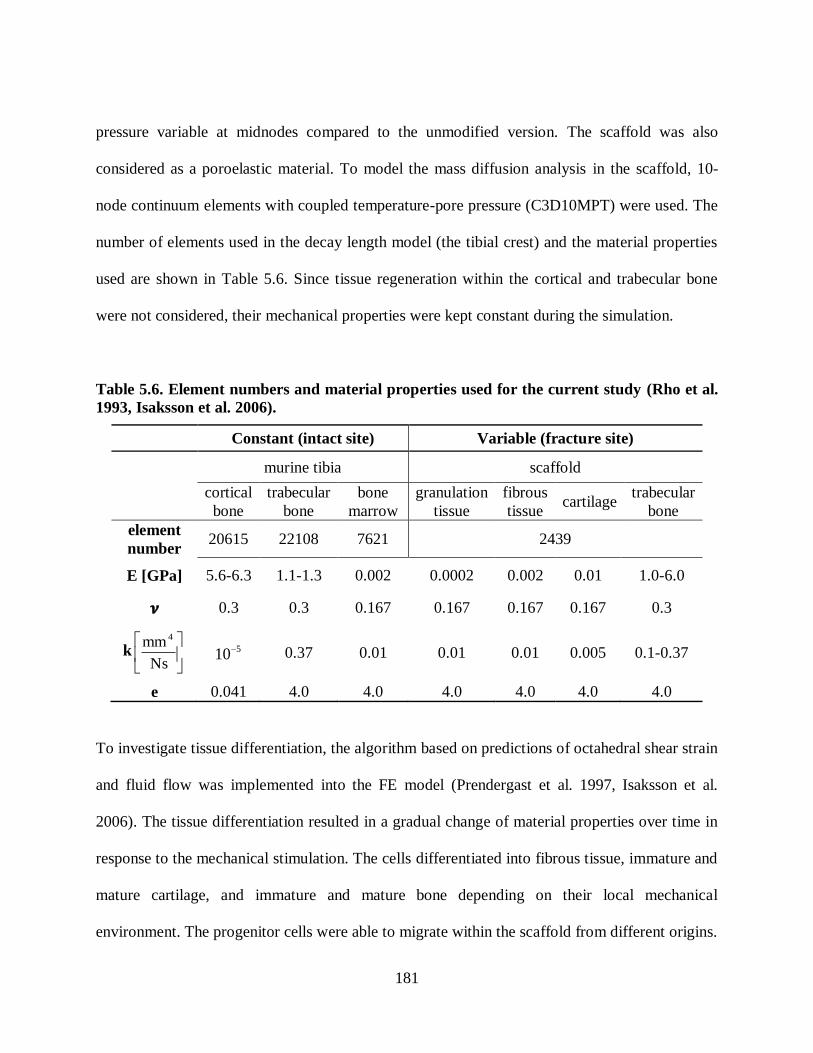
181

pressure variable at midnodes compared to the unmodified version. The scaffold was also

considered as a poroelastic material. To model the mass diffusion analysis in the scaffold, 10-

node continuum elements with coupled temperature-pore pressure (C3D10MPT) were used. The

number of elements used in the decay length model (the tibial crest) and the material properties

used are shown in Table 5.6. Since tissue regeneration within the cortical and trabecular bone

were not considered, their mechanical properties were kept constant during the simulation.

Table 5.6. Element numbers and material properties used for the current study (Rho et al.

1993, Isaksson et al. 2006).


murine tibia scaffold

cortical

bone

trabecular

bone

bone

marrow

granulation

tissue

fibrous

tissue cartilage

trabecular

bone

element

number 20615 22108 7621 2439

E [GPa] 5.6-6.3 1.1-1.3 0.002 0.0002 0.002 0.01 1.0-6.0

0.3 0.3 0.167 0.167 0.167 0.167 0.3

k

Ns

mm 4

510 0.37 0.01 0.01 0.01 0.005 0.1-0.37

e 0.041 4.0 4.0 4.0 4.0 4.0 4.0

To investigate tissue differentiation, the algorithm based on predictions of octahedral shear strain

and fluid flow was implemented into the FE model (Prendergast et al. 1997, Isaksson et al.

2006). The tissue differentiation resulted in a gradual change of material properties over time in

response to the mechanical stimulation. The cells differentiated into fibrous tissue, immature and

mature cartilage, and immature and mature bone depending on their local mechanical

environment. The progenitor cells were able to migrate within the scaffold from different origins.

182

A user-defined subroutine USDFLD was developed to update the material properties based on

the average of computed mechanical stimuli in the previous 10 days. The rule of mixtures was

used to al ulate the new material properties (Young‟s modulus, oisson‟s ratio and

permeability). In each iteration, the mechanical stimuli were calculated at the maximum loading.

The simulation continued until the tissue distribution in the scaffold reached a steady state.

5.5.1 Investigation of axial compression load

The decay length model (the tibial crest) of the reconstructed murine tibia with a 0.7 mm fracture

gap was used to represent a closed burr-hole fracture model (Figure 5.12) (Taiani 2012). Tissue

differentiation patterns were investigated for 2, 1 and 0.5 N (1 Hz) compression loads applied to

the proximal end of the tibia. The distributed loading was selected to avoid stress concentration.

Since the hole was created in the trabecular bone (2.55 mm from the proximal site), the

progenitor cells could migrate into the fracture site from two origins: (1) the surrounding muscle

tissues, and (2) the endosteum (Figure 5.21a). The diffusion coefficients were set such that after

21 days (steps) the progenitor cells would spread throughout the entire fracture zone (Gardner et

al. 2006). Each step represented the average load that had been applied to the bone during one

day of healing (Isaksson et al. 2006).

The granulation tissue gradually differentiated into stiffer tissues over time. Therefore, by

stiffening the scaffold the mechanical stimuli decreased and the interfragmentary gap movement

reached a steady state (Figure 5.23). The tissue distribution changed over time due to the change

of mechanical stimuli and cell concentration. The model predicted an increase in the mechanical

stimuli in cell seeded scaffold in the first few days (days 1-3). Thereafter, the octahedral shear

strain started to reduce while the fluid velocity decreased more gradually (days 4-8) and then

reached a steady state (days 9-21) (Figure 5.22). The predicted magnitudes of the mechanical

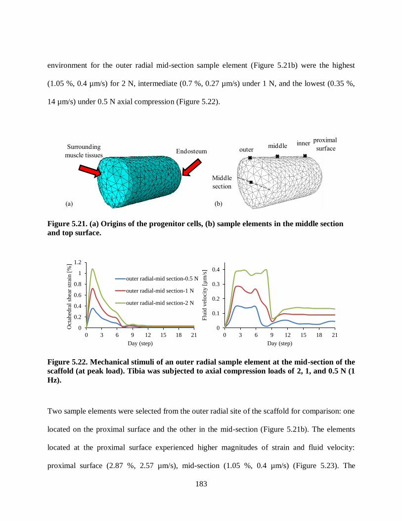
183

environment for the outer radial mid-section sample element (Figure 5.21b) were the highest

(1.05 %, 0.4 µm/s) for 2 N, intermediate (0.7 %, 0.27 µm/s) under 1 N, and the lowest (0.35 %,

14 µm/s) under 0.5 N axial compression (Figure 5.22).

Surrounding

muscle tissuesEndosteum

proximal

surface

Middle

section

outermiddle inner

(a) (b)

Figure 5.21. (a) Origins of the progenitor cells, (b) sample elements in the middle section

and top surface.

0

0.2

0.4

0.6

0.8

1

1.2

0 3 6 9 12 15 18 21

Oct

ahed

ral

shea

r st

rain

[%

]

Day (step)

outer radial-mid section-0.5 N

outer radial-mid section-1 N


0

0.1

0.2

0.3

0.4

0 3 6 9 12 15 18 21

Flu

id v

eloci

ty [

µm

/s]

Day (step)

Figure 5.22. Mechanical stimuli of an outer radial sample element at the mid-section of the

scaffold (at peak load). Tibia was subjected to axial compression loads of 2, 1, and 0.5 N (1

Hz).

Two sample elements were selected from the outer radial site of the scaffold for comparison: one

located on the proximal surface and the other in the mid-section (Figure 5.21b). The elements

located at the proximal surface experienced higher magnitudes of strain and fluid velocity:

proximal surface (2.87 %, 2.57 µm/s), mid-section (1.05 %, 0.4 µm/s) (Figure 5.23). The

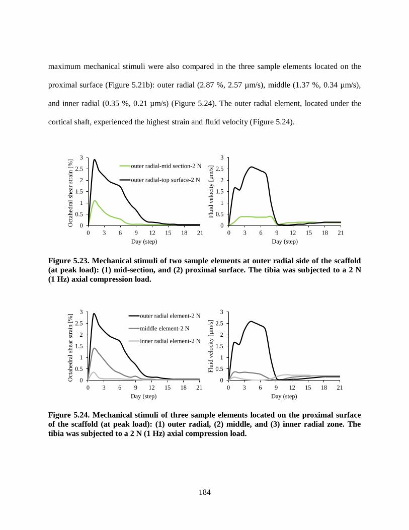
184

maximum mechanical stimuli were also compared in the three sample elements located on the

proximal surface (Figure 5.21b): outer radial (2.87 %, 2.57 µm/s), middle (1.37 %, 0.34 µm/s),

and inner radial (0.35 %, 0.21 µm/s) (Figure 5.24). The outer radial element, located under the

cortical shaft, experienced the highest strain and fluid velocity (Figure 5.24).

0

0.5

1

1.5

2

2.5

3

0 3 6 9 12 15 18 21

Oct

ahed

ral

shea

r st

rain

[%

]

Day (step)


outer radial-top surface-2 N

0

0.5

1

1.5

2

2.5

3

0 3 6 9 12 15 18 21

Flu

id v

eloci

ty [

µm

/s]

Day (step)

Figure 5.23. Mechanical stimuli of two sample elements at outer radial side of the scaffold

(at peak load): (1) mid-section, and (2) proximal surface. The tibia was subjected to a 2 N

(1 Hz) axial compression load.

0

0.5

1

1.5

2

2.5

3

0 3 6 9 12 15 18 21

Oct

ahed

ral

shea

r st

rain

[%

]

Day (step)

outer radial element-2 N

middle element-2 N

inner radial element-2 N

0

0.5

1

1.5

2

2.5

3

0 3 6 9 12 15 18 21

Flu

id v

elo

city

[µ

m/s

]

Day (step)

Figure 5.24. Mechanical stimuli of three sample elements located on the proximal surface

of the scaffold (at peak load): (1) outer radial, (2) middle, and (3) inner radial zone. The

tibia was subjected to a 2 N (1 Hz) axial compression load.

185

During the fracture healing period, the interfragmentary strain was calculated for the three

loading cases under the cortical shaft as follows:

gap

3

entaryinterfragml

Δuε . 5.4

where entaryinterfragmε was the interfragmentary strain, 3Δu was the interfragmentary motion in axial

direction, and gapl was the gap size of 0.7 mm. The 2 N loading case had the maximum

interfragmentary strain (0.3 %) whereas the 1 and 0.2 N loading cases had the strains of 0.2 and

0.1, respectively (Figure 5.25).

0

0.05

0.1

0.15

0.2

0.25

0.3

0 3 6 9 12 15 18 21

Inte

rfra

gm

enta

ry s

trai

n [

%]

Day (step)

0.5 N 1 N 2 N

Figure 5.25. The predicted interfragmentary strain, at peak load, under the cortical shaft

for the three loading cases (2, 1, 0.5 N axial compression, 1 Hz).

The predicted healing patterns are shown in Figure 5.26. In all cases, the bone formation initiated

from the outer edges of the scaffold and gradually proceeded the inner regions. The 0.5 N

loading case had accelerated healing compared to others (e.g., see day 11 in Figure 5.26), which

was due to the lower mechanical stimuli that the elements were experiencing in the 0.5 N loading

case. However, under 0.5 N axial compression load, the mechanical stimuli had only a marginal

186

amount of bone formation at the inner radial location of the scaffold and fibrous tissue was still

present (0.5 N, Day 14, Figure 5.26), while for the two other cases bony tissue was formed (2

and 1 N, Day 14, Figure 5.26).

fibrous tissue immature cartilage mature cartilage immature bone mature bone

0.5 N

1 N

2 N

Day 6 Day 9 Day 12

Day 6 Day 11

Day 14

Day 9

Day 9Day 6 Day 11

Day 11

Day 12

Day 12

Day 14

Day 14

Figure 5.26. Predicted fracture healing patterns under the 2, 1 and 0.5 N (1 Hz) axial

compression load.

For all of the axial loading cases, bony tissue started to form from both proximal and distal sides,

which may be due to the initially higher concentration of progenitor cells at those regions

compared to other zones (i.e. outer and inner radial sides of the scaffold were the origins of the

progenitor cells). In the 2 N loading case, the inner radial side had increased healing compared to

the middle and outer radial sides. This may be due to the lower mechanical stimuli at the inner

radial (e.g. strain on day 11, inner: 0.0096 %, middle: 0.05 %, outer: 0.18 %, Figure 5.24), (2 N,

Days 11-14, Figure 5.26). On day 12 (2 N) the zone under the cortical shaft had differentiated

into cartilaginous tissue and bony tissue did not form. This showed the zone under the cortical

187

shaft was subjected to higher magnitudes of displacement, strain and fluid velocity (e.g. day 12

strain, outer: 0.14 %, middle: 0.03 %, inner: 0.0094 %, Figure 5.24).

The core of the scaffold had an increased rate of healing compared to the outer layers (Figure

5.27). For the 2 N loading case the inner core had differentiated into mature cartilage at day 10

(Day 10, Figure 5.27) whereas the outer layer was still immature cartilage. On day 11, the inner

tissue had differentiated into immature bone whereas the outer layer was still cartilaginous (Day

11, Figure 5.27). The same sequence could be observed for differentiation into mature and

immature bone for the inner core compared to the outer layers of the scaffold (Days 12-14,

Figure 5.27). This may be due to higher mechanical stimuli at the outer layers compared to the

core (e.g. on day 13 strain, outer layer: 0.12 %, core: 0.04 %) (Figure 5.23).

immature cartilage mature cartilage immature bone mature bone

Day 11Day 10 Day 12 Day 13 Day 14

Figure 5.27. Cross-sectional view of the scaffold showing the accelerated healing of the core

compared to the outer layers. The tibia was subjected to a 2 N (1 Hz) axial compression

load.

5.5.2 Influence of cell diffusivity rate

To investigate the effect of cell diffusion rate, two magnitudes of mass diffusivity were

investigated and the healing patterns compared. The burr-hole fracture model with a 0.7 mm gap

located in the trabecular bone (2.55 mm from the proximal end) was used (Figure 5.12). The

proximal end of the tibia was subjected to a cyclic 1 N (1 Hz) axial compression load and the cell

188

diffusivities were set 0.025 and 0.01 s

mm 2

. The higher diffusion constant (0.025 s

mm2

)

represented a younger bone compared to the 0.01 s

mm2

case (Geris et al. 2009). Mice fractures

generally heal by 21 days (Gardner et al, 2006). Using the diffusive rate of 0.025 s

mm2

, the

progenitor cells could spread throughout the entire scaffold after 3 weeks (21 steps). On the other

hand, the diffusive rate of 0.01 s

mm2

, represented a lower diffusion in which cells were partially

spread through the scaffold after 21 days. The progenitor cells were able to migrate faster in the

model with a higher mass diffusion constant. The octahedral shear strain was computed for the

middle sample element at the proximal surface in both models (Figure 5.21b, Figure 5.28). The

octahedral shear strain was similar in the initial stages indicating that the cell concentration did

not differ greatly at the beginning of the analysis (Figure 5.28). However, the cells migrated

quicker to the middle zone in the model with a higher diffusivity (0.025 s

mm2

) and the rate of

differentiation was accelerated (Figure 5.29). The model with a high diffusion rate led to a stiffer

matrix in the scaffold and thus lower octahedral shear strain (Figure 5.28). The healing pattern

showed that both models had the same tissue patterns in the initial stages (Day 6, Figure 5.29).

However, in the higher diffusion case, bone had formed by day 14 whereas the fracture site was

still cartilaginous in the lower diffusion case (Figure 5.29).

During aging, the ability of bone to recruit progenitor cells is reduced (Bailón-Plaza and van der

Meulen 2003, Geris et al. 2009). This partly explains why fractures heal quicker in youth than in

adults (Bailón-Plaza and van der Meulen 2003, Geris et al. 2009). The sensitivity of the cells to

189

mechanical perturbations is reduced (Lang 2011). In agreement with the literature, the fracture

healed quicker in the young bone (with higher diffusion rate) compared to the older bone with

lower diffusion rate (Figure 5.29).

0

0.2

0.4

0.6

0.8

1

0 3 6 9 12 15 18

Oct

ahh

edra

l sh

ear

stra

in [

%]

Day (step)

D = 0.01 D= 0.025

Figure 5.28. The prediction of octahedral shear strain for different cell diffusion rates

(0.025 and 0.01 s

mm2

).

granulation tissue fibrous tissue immature cartilage mature cartilage immature bone mature bone

D = 0.025



D = 0.01

Day 7

Day 7 Day 9

Day 9 Day 11

Day 11 Day 12

Day 12 Day 14

Day 14

Figure 5.29. Predicted fracture healing patterns under the 1 N (1 Hz) axial compression

load for different rates of cell diffusion (0.025 and 0.01 s

mm2

).

190

5.5.3 Influence of fracture position

To determine the effect of fracture position on healing two parametric studies were performed:

1. The position of fractures differed axially, but both were located in the trabecular bone to

explore the effect of changes in mechanical stimuli on tissue differentiation.

2. The position of fractures differed axially, with one located in the trabecular bone and the

other located in the bone marrow. In these cases, both the number of progenitor cells and

the mechanical stimuli differed.

5.5.3.1 Different mechanical stimuli with the same cell origins

To investigate the effect of fracture position on the healing rate two different burr-hole fractures

with the same diameter (0.7 mm) were created in the trabecular bone (both had the same cell

origins and diffusivity). The holes were located at different axial positions with respect to the

proximal end of the tibiae: 2.55 mm versus 3.13 mm (Figure 5.30). An axial compression load of

1 N (1 Hz) was applied to the proximal end of the tibia and the predicted healing patterns were

contrasted for the two models.

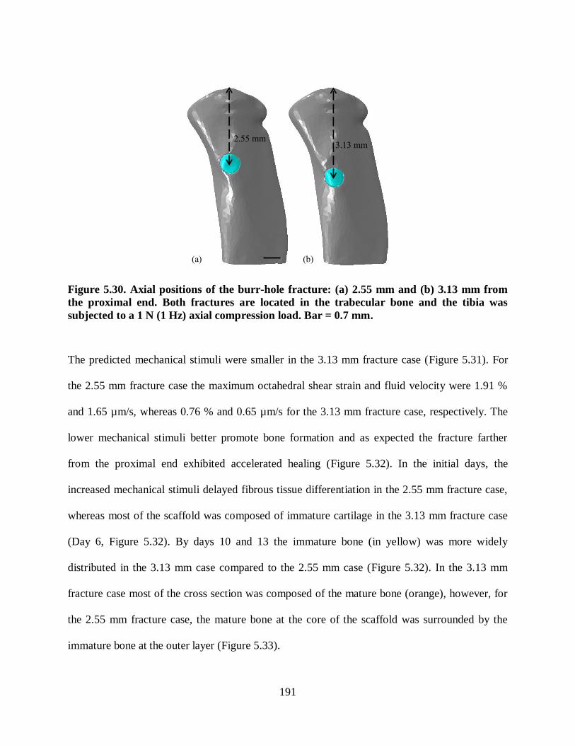
191

2.55 mm3.13 mm

(a) (b)

Figure 5.30. Axial positions of the burr-hole fracture: (a) 2.55 mm and (b) 3.13 mm from

the proximal end. Both fractures are located in the trabecular bone and the tibia was

subjected to a 1 N (1 Hz) axial compression load. Bar = 0.7 mm.

The predicted mechanical stimuli were smaller in the 3.13 mm fracture case (Figure 5.31). For

the 2.55 mm fracture case the maximum octahedral shear strain and fluid velocity were 1.91 %

and 1.65 µm/s, whereas 0.76 % and 0.65 µm/s for the 3.13 mm fracture case, respectively. The

lower mechanical stimuli better promote bone formation and as expected the fracture farther

from the proximal end exhibited accelerated healing (Figure 5.32). In the initial days, the

increased mechanical stimuli delayed fibrous tissue differentiation in the 2.55 mm fracture case,

whereas most of the scaffold was composed of immature cartilage in the 3.13 mm fracture case

(Day 6, Figure 5.32). By days 10 and 13 the immature bone (in yellow) was more widely

distributed in the 3.13 mm case compared to the 2.55 mm case (Figure 5.32). In the 3.13 mm

fracture case most of the cross section was composed of the mature bone (orange), however, for

the 2.55 mm fracture case, the mature bone at the core of the scaffold was surrounded by the

immature bone at the outer layer (Figure 5.33).

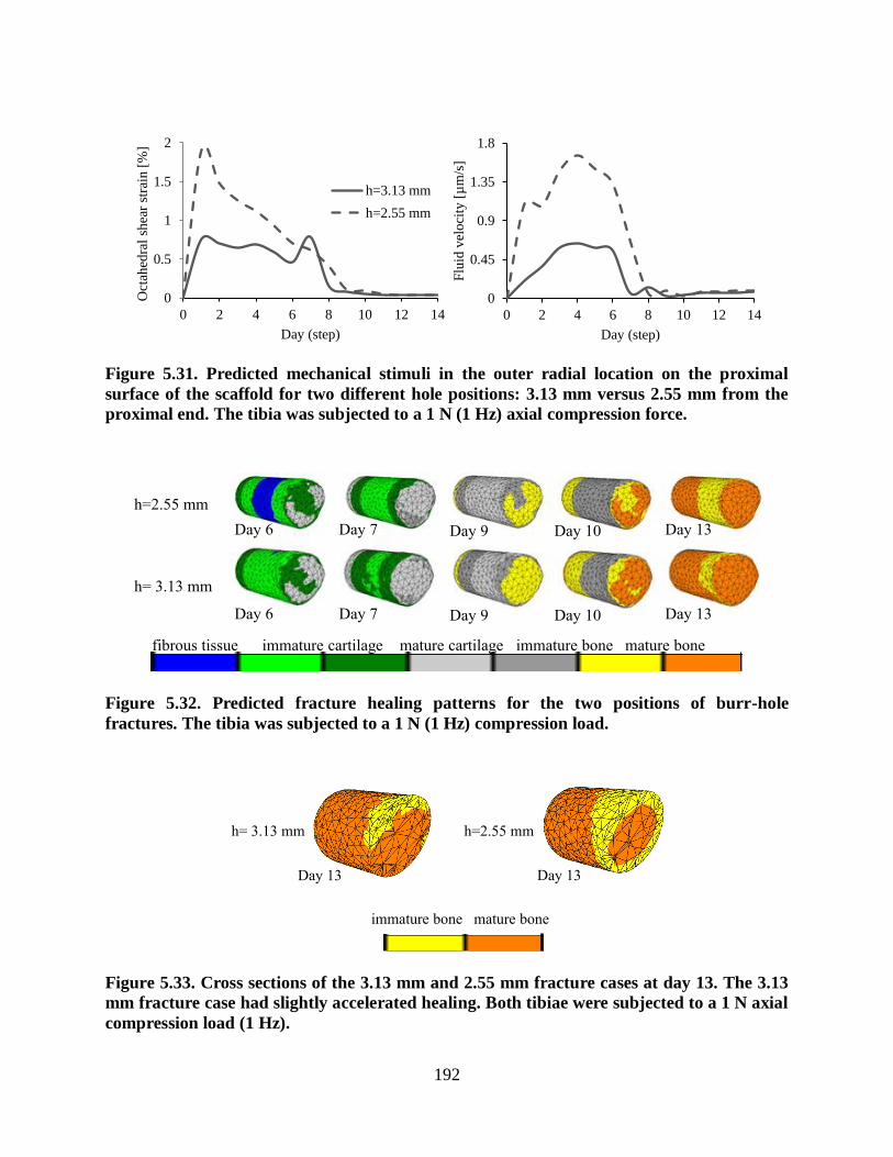
192

0

0.5

1

1.5

2

0 2 4 6 8 10 12 14

Oct

ahed

ral

shea

r st

rain

[%

]

Day (step)

h=3.13 mm

h=2.55 mm

0

0.45

0.9

1.35

1.8

0 2 4 6 8 10 12 14

Flu

id v

eloci

ty [

µm

/s]

Day (step)

Figure 5.31. Predicted mechanical stimuli in the outer radial location on the proximal

surface of the scaffold for two different hole positions: 3.13 mm versus 2.55 mm from the

proximal end. The tibia was subjected to a 1 N (1 Hz) axial compression force.


h=2.55 mm



h= 3.13 mm

Figure 5.32. Predicted fracture healing patterns for the two positions of burr-hole

fractures. The tibia was subjected to a 1 N (1 Hz) compression load.

immature bone mature bone

h=2.55 mm

Day 13Day 13

h= 3.13 mm

Figure 5.33. Cross sections of the 3.13 mm and 2.55 mm fracture cases at day 13. The 3.13

mm fracture case had slightly accelerated healing. Both tibiae were subjected to a 1 N axial

compression load (1 Hz).

193

5.5.3.2 Different mechanical stimuli and cell origins

To investigate the effect of both fracture position and origin of progenitor cells on the healing

rate, two different burr-hole fractures with the same diameter (0.7 mm) were created in the

trabecular bone (case A) and bone marrow (case B). The fracture located in the trabecular bone

had 2 cell origins (Figure 5.21a) whereas the one within the bone marrow had three cell origins

(Figure 5.34). The holes were located at different axial positions with respect to the proximal end

of the tibiae: 2.55 mm versus 4.95 mm. An axial compression load of 2.5 N (1 Hz) was applied

to the proximal end of the tibia. A higher load magnitude (2.5 N instead of 1 N) was used to

ensure the mechanical stimuli within the 4.95 mm fracture case was not negligible and was

adequate to stimulate the tissue differentiation. The octahedral shear strain and fluid velocity

were negligible in the initial days and increased over time in case B. Then with stiffening of the

scaffold, the mechanical stimuli decreased gradually and reached a steady state (Figure 5.35).

Surrounding

muscle tissuesEndosteum

Bone marrow

Figure 5.34. The origins of progenitor cells when the fracture is located in the bone

marrow.

194

0

1

2

3

4

5

0 3 6 9 12 15 18

Oct

ahed

ral

shea

r st

rain

[%

]

Day (step)

Trabecular bone

Bone marrow

0

0.5

1

1.5

2

2.5

3

3.5

4

4.5

0 3 6 9 12 15 18

Flu

id v

eloci

ty [

µm

/s]

Day (step)

Figure 5.35. Predicted mechanical stimuli for two locations of the fracture (outer radial

sample element on the proximal surface): (1) in trabecular bone and (2) in bone marrow.

Tibia was subjected to a 2.5 N (1 Hz) compression load.

The predicted patterns of tissue differentiation showed that healing accelerated in Case B (Figure

5.36). By day 6 considerable amounts of fibrous tissue existed in the scaffold for case A,

however, in case B immature and mature cartilage were already observed (Day 6, Figure 5.36).

After 13 days, cartilaginous tissue still existed under the cortical shaft of case A, whereas tissue

had differentiated into bone in case B. This may be due to the lower mechanical stimuli,

particularly fluid velocity, and the higher concentration of progenitor cells in case B. Since the

progenitor cells originated from three origins in case B, the cells migrated through the fracture

site faster than case A (with only two cell origins). Therefore, a greater source of progenitor cells

accelerated the healing period (Figure 5.36).

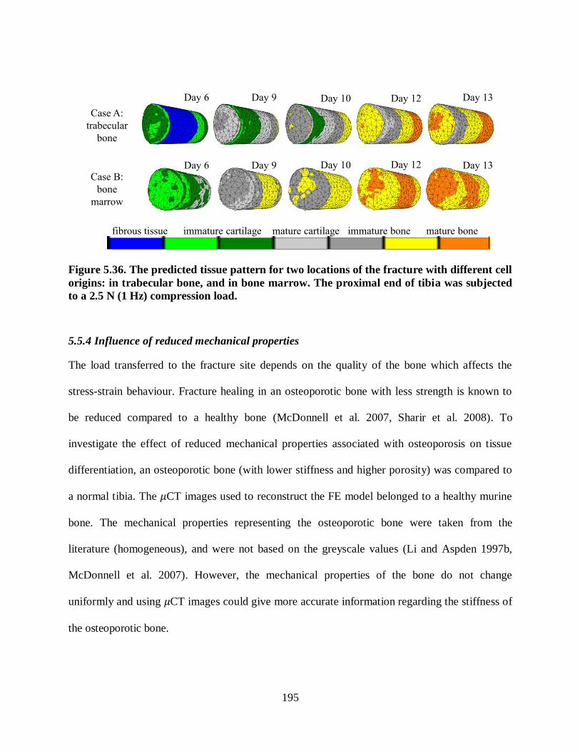
195


Case A:

trabecular

bone



Case B:

bone

marrow

Figure 5.36. The predicted tissue pattern for two locations of the fracture with different cell

origins: in trabecular bone, and in bone marrow. The proximal end of tibia was subjected

to a 2.5 N (1 Hz) compression load.

5.5.4 Influence of reduced mechanical properties

The load transferred to the fracture site depends on the quality of the bone which affects the

stress-strain behaviour. Fracture healing in an osteoporotic bone with less strength is known to

be reduced compared to a healthy bone (McDonnell et al. 2007, Sharir et al. 2008). To

investigate the effect of reduced mechanical properties associated with osteoporosis on tissue

differentiation, an osteoporotic bone (with lower stiffness and higher porosity) was compared to

a normal tibia. The CT images used to reconstruct the FE model belonged to a healthy murine

bone. The mechanical properties representing the osteoporotic bone were taken from the

literature (homogeneous), and were not based on the greyscale values (Li and Aspden 1997b,

McDonnell et al. 2007). However, the mechanical properties of the bone do not change

uniformly and using CT images could give more accurate information regarding the stiffness of

the osteoporotic bone.

196

The Young‟s modulus of the orti al one was al ulated using a relation etween the stiffness

and density of the osteoporotic bone as follows (Li and Aspden 1997a):

22.1ρ21.4E . 5.5

where ρ = 1.02 is the density 3cmgr

and E is the Young‟s modulus [G a].

The Young‟s modulus and void ratio of the orti al one were assumed to e 1.23 G a and 0.22

for osteoporotic bone (Li and Aspden 1997b, McDonnell et al. 2007). A value of 0.4 GPa and 11

were used for the Young‟s modulus and void ratio of the tra e ular one (Sun et al. 2008). The

permeability of the osteoporotic trabecular and cancellous bone were selected based on a

parametric study performed by Lacroix (2000). In this parametric study, three different

magnitudes of permeability were used (high, middle and low) to find the best to represent normal

bone. The middle value was selected to represent the permeability of the normal bone (Lacroix

2000). Since the osteoporotic bone had greater porosity the highest values were selected for

cortical (0.001 Ns

mm 4

) and trabecular bone (0.5 Ns

mm 4

) (McDonnell et al. 2007). The oisson‟s

ratio of an osteoporotic murine tibia was not available in the literature; a oisson‟s ratio similar

to that of a healthy bone was used. However, further research is needed to obtain more realistic

values for the oisson‟s ratio. The me hani al properties used for the osteoporoti one are

shown in Table 5.7.

A model of the murine tibia with a 0.7 mm fracture gap at an axial distance of 2.55 mm from the

proximal end of the tibia was used (Figure 5.12) (Taiani 2012). An axial compression load of 2.5

N (1 Hz) was applied to the proximal end of the tibia to simulate the running (De Souza et al.

2005, Stadelmann et al. 2009, Prasad et al. 2010). The fracture was located in the trabecular

197

bone, and surrounding muscle tissues and endosteum were considered as the two origins of

progenitor cells in both cases. The mechanical stimuli, interfragmentary strain and healing

patterns were compared between normal and osteoporotic bone (Figure 5.39-5.39).



values can be contrasted to those for healthy bone in Table 5.6.


murine tibia scaffold

cortical

bone

trabecular

bone

bone

marrow

granulation

tissue

fibrous

tissue cartilage

trabecular

bone

element

number 20615 22108 7621 2439

E [GPa] 1.23 0.4 0.002 0.0002 0.002 0.01 1.0-6.0

0.3 0.3 0.167 0.167 0.167 0.167 0.3

k

Ns

mm 4

310 0.5 0.01 0.01 0.01 0.005 0.1-0.37

e 0.22 8.1 4.0 4.0 4.0 4.0 4.0

The maximum octahedral shear strain and fluid velocity within the fracture were much higher in

the osteoporotic bone compared to the normal bone (Figure 5.37). This may be explained by

much lower stiffness, higher permeability and void ratio of the surrounding osteoporotic bone.

The octahedral shear strain and fluid velocity were 14 % and 8.5 µm/s for the osteoporotic bone

and only 4.8 % and 4.3 µm/s for the normal bone, respectively (Figure 5.37). The

interfragmentary strain was also calculated for the fracture gap (under the cortical shaft). The

interfragmentary strain within the osteoporotic bone was 4.6 times higher than in the normal

bone (Figure 5.38). The higher values of mechanical stimuli increased the motion within the

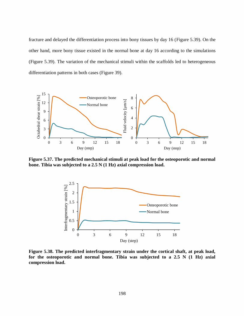
198

fracture and delayed the differentiation process into bony tissues by day 16 (Figure 5.39). On the

other hand, more bony tissue existed in the normal bone at day 16 according to the simulations

(Figure 5.39). The variation of the mechanical stimuli within the scaffolds led to heterogeneous

differentiation patterns in both cases (Figure 39).

0

3

6

9

12

15

0 3 6 9 12 15 18

Oct

ahed

ral

shea

r st

rain

[%

]

Day (step)

Osteoporotic bone

Normal bone

0

2

4

6

8

0 3 6 9 12 15 18

Flu

id v

eloci

ty [

µm

/s]

Day (step)

Figure 5.37. The predicted mechanical stimuli at peak load for the osteoporotic and normal

bone. Tibia was subjected to a 2.5 N (1 Hz) axial compression load.

0

0.5

1

1.5

2

2.5

0 3 6 9 12 15 18

Inte

rfra

gm

enta

ry s

trai

n [

%]

Day (step)

Osteoporotic bone

Normal bone

Figure 5.38. The predicted interfragmentary strain under the cortical shaft, at peak load,

for the osteoporotic and normal bone. Tibia was subjected to a 2.5 N (1 Hz) axial

compression load.

199

The fracture site (scaffold) of the osteoporotic bone was filled mainly with the fibrous tissue in

the initial stages of healing (day 7), whereas the fibrous tissue had differentiated into

cartilaginous tissue in the normal bone at day 7 (Figure 5.39). The fracture model of the normal

tibia had accelerated healing compared to the osteoporotic bone. The delayed healing of the

osteoporotic bone may be due to higher magnitudes of mechanical stimuli at fracture site (Figure

5.37).


Normal



Osteoporotic

Figure 5.39. The predicted tissue patterns for fracture repair within osteoporotic versus

normal bone. Tibia was subjected to a 2.5 N (1Hz) axial compression load.

5.5.5 Influence of bending load

To explore the effect of bending load, 2 (0.04 Nm, 1 Hz) and 1 N (0.02 Nm, 1 Hz) posteriorly

directed loads were applied to the proximal tibia to cause bending (0.04, 0.02 Nm). The model of

a burr-hole fracture with a 0.7 mm gap located in the trabecular bone (2.55 mm from the

proximal point) was used (Figure 5.40). The mechanical stimuli were compared for both loading

cases. Since the bone was subjected to a lower bending load in the 0.02 Nm, the case mechanical

stimuli were lower (Figure 5.41). The fracture stiffened in both cases over time and the

mechanical stimuli reached a steady state by day 11 (Figure 5.41, Figure 5.42). The fracture

200

region in the bone for the 0.02 Nm case had differentiated into immature bone by day 10 whereas

the 0.04 Nm loading still contained cartilaginous tissue. By day 11 most of the fracture site had

differentiated into mature bone in the 0.02 Nm case, whereas for the 0.04 Nm case cartilaginous

tissue as well as immature bone were existed (Figure 5.41). This indicated that the higher

mechanical bending load might lead to a delay in tissue differentiation and fracture healing.

Figure 5.40. Red arrow shows the bending load that was applied to the tibia. The distal end

was fixed and the hole size was 0.7 mm. Bar = 0.7 mm.

201

0

0.1

0.2

0.3

0.4

0.5

0.6

0 3 6 9 12 15 18 21 24

Oct

ahed

ral s

hea

r st

rain

[%

]

Day (step)

0.02 Nm

0.04 Nm

0

0.1

0.2

0.3

0.4

0.5

0.6

0.7

0.8

0 3 6 9 12 15 18 21 24

Flu

id v

elo

city

[µ

m/s

]

Day (step)

Figure 5.41. Predicted mechanical stimuli for the outer radial sample element at located at

the proximal surface of the scaffold. The tibia was subjected to 0.04 and 0.02 Nm (1 Hz)

bending loads.


0.02 N



0.04 N

Figure 5.42. Predicted tissue pattern for the murine tibia subjected to bending loads of 0.04

and 0.02 Nm (1 Hz).

5.6 Summary and discussion

A µCT based FE model of a murine tibia was developed to investigate the healing patterns in a

burr-hole fracture model. Greyscale-based material properties were used for the cortical and

trabecular tissues. Initially, the mechanical behaviour of the intact tibia was verified against a

previous experimental-numerical study (Stadelmann et al. 2009). Thereafter, burr-hole fracture

models were created to investigate the tissue differentiation within the fracture site under

202

different conditions (axial compression load, diffusivity rate, fracture position, osteoporotic bone

and bending load) using the biphasic mechanoregulatory algorithm (Lacroix et al. 2002).

Accelerated fracture healing was predicted in conditions where the tibia was subjected to lower

magnitude of axial compression load (0.5 N, 1 Hz), which was in agreement with the previous

experimental study of Gardner et al. (2006). When tibia was subjected to higher loads (2, 1 N, 1

Hz), the bone formation was delayed and the fracture site was composed of less bony tissue.

Hence, the stiffness of the scaffold under the 0.5 N axial compression load was higher than other

cases. The axial compression loads of 2 and 1 N (1 Hz) produced strains at the fracture site,

which were higher than the threshold values proposed by Prendergast et al. (1997) and were not

appropriate for bone differentiation. The elements located at the outer layer of the scaffold were

exposed to higher range of mechanical stimuli (Figure 5.23), and therefore tissue differentiation

was delayed (Figure 5.27). The magnitudes of mechanical stimuli regulated healing pathways

within different regions of the scaffold and the differentiation of the bony tissue initiated from

regions that experienced less mechanical stimuli (the core of the scaffold). There were

inadequate histological slides or CT images to show where the bony tissue was initially formed

at the fracture. He et al. (2011) investigated the fracture repair in a burr-hole murine femur (in

vivo), and was shown that in the formation of bone initiated from outer layers. Unlike our case

that the fracture site was filled with a stem cell seeded scaffold, the burr-hole in the murine

femur had not been filled with a scaffold and the fracture was supposed to heal on its own (He et

al. 2011). The existence of the scaffold and different loading condition in our model may

resulted the difference in the regions that bony tissue was initially formed.

203

To investigate the effect of cell diffusion rate, the healing progression was compared using

different rates of diffusivity (young murine: D=0.025 s

mm 2

and old murine: D=0.01

s

mm 2

).

Initially all of the elements were assumed to be composed of granulation tissue (E=0.2 MPa).

During the healing period, the stiffness of the elements was gradually increased by

differentiating into fibrous tissue, cartilaginous tissue or bony tissue (Figure 5.43). The stiffness

of the scaffold was computed using the rule of mixtures for each day (step) of healing (Figure

5.44). In both cases, a gradual increase in the stiffness of the scaffold was observed during the

healing period; however, the model with a higher rate of cell migration had accelerated healing

compared to the model with a slower rate of cell migration (Figures 5.43-44). The computational

predictions were compared qualitatively with the experimental results from Lu et al. (2005),

which investigated the healing progression of closed fractures in young and adult murine tibia. In

the experimental study, the mice were able to move freely after the injury. The histological slides

and molecular analyses showed that the elder mice had a delayed endochondral ossification and

required a longer healing period (Figure 5.45a-b, Lu et al. 2005). However, younger mice with

higher concentration of progenitor cells were more metabolically active and had a faster fracture

healing. At day 7, Lu et al. (2005) observed a large amount of cartilaginous tissue in the

histological slide of the younger mice. The computational simulation also predicted a small

amount of cartilaginous tissue presented in the older murine by Day 7 (Figure 5.45). Both

computational and in vivo studies, predicted an accelerated healing for the juvenile tibiae. The

experimental and computational data suggested that the rate of cell diffusion affected the healing

process. Therefore, increasing the rate of diffusion in elderly patients may promote the process of

mineralisation and fracture repair and may lead to development of novel treatments.

204

Mature bone

Fibrous tissue

Cartilage

Immature bone

Granulation tissue0

0.5

1

1.5

2

2.5

3

3.5

4

0 2 4 6 8 10 12 14 16 18

Day (step)

D=0.025 D=0.01

Figure 5.43. The gradual change of tissue type during the healing period within a young

(D=0.025 s

mm 2

), and an old murine tibia (D=0.01 s

mm 2

).

Figure 5.44. The overall stiffness of the scaffold during the healing process for young and

old murine tibia with different diffusion rates (D=0.025 s

mm 2

and D=0.01

s

mm 2

).

205

(c) (d)

granulation fibrous tissue immature /mature cartilage

Young Old

Day 7 Day 7 (Lu et al., 2005)

Young Old

Day 7 Day 7 (Lu et al., 2005)

OldYoung

(a) (b)

Young Old

Figure 5.45. Histological slides (Day 7): (a) a large and (b) a small amount of cartilage were

present in the fracture site of young and elder murine tibia, respectively. In the histological

slides, cartilage is shown in red (Lu et al. 2005). In the computational study (Day 7)

similarly, more cartilaginous tissue differentiated in the younger murine tibia (c, d).

Two models with different fracture positions but same number of cell origins were created to

explore the effect of fluid velocity and octahedral shear strain on the healing process. The

fracture models were located 2.55 mm and 3.13 mm from the proximal tibia and the cells

migrated into the fracture site from endosteum and surrounding muscle tissues. The fracture

located further from the proximal tibia (3.13 mm) was predicted to have an accelerated healing

compared to the 2.55 mm case. Since the cell rate and cell origin were the same in both models,

higher magnitudes of strain and fluid velocity within the scaffold might resulted in a delayed

fracture healing process in the 2.55 mm case (Figures 5.31-32). Another fracture model was

created with three cell origins (endosteum, surrounding muscle tissues and bone marrow) in the

4.95 mm distance from the proximal tibia. The predictions showed that the healing was

accelerated in the model located in bone marrow cavity with higher cell concentration and lower

mechanical stimuli through the healing process (Figure 5.35). There were no histological slides

available to compare to computational results.

The osteoporotic bone, with a lower bone stiffness surrounding the fracture, plus a higher

permeability and void ratio, had delayed healing compared to the normal tibia. The rate of

diffusivity was kept constant, in both normal and osteoporotic cases, to solely investigate the

206

effect of mechanical properties on tissue differentiation. The FE model of the closed burr-hole

fracture was created based on a in vivo study (Taiani et al. 2010). The stiffness of the scaffolds

were calculated during the healing process using the computational simulations. The scaffold

stiffness gradually increased over time in both normal and osteoporotic murine tibia (Figure

5.46); however, the overall stiffness of the fracture site within the normal tibia was higher

(Figures 5.39, 5.47). The computational predictions showed that the normal tibia had promoted

fracture healing compared to the osteoporotic case. This was in agreement with experimental

observations that the osteoporotic bones are difficult to heal (Taiani 2012, He et al. 2011). The

CT images from Taiani et al. (2012) and the computational predictions both indicate that the

osteoporotic tibia had less mineralisation compared to the normal case (Figures 5.39, 5.48). He et

al. (2011) created burr-hole fracture models in mice femur to analyse the healing process in

normal and osteoporotic bones, and the CT images from the osteoporotic bone showed a

delayed healing.

Figure 5.46. The gradual change of tissue type during the healing period within a normal

and an osteoporotic murine tibia.

207

Figure 5.47. The overall stiffness of the scaffold during the healing process for normal and

osteoporotic bone.

Normal

Osteoporotic (Taiani, 2012)

Day 0 Day 7 Day 14 Day 28

1 mm

Figure 5.48. The healing progression in a normal bone and an osteoporotic bone from CT

images show that the normal bone had more mineralisation (Taiani 2012).

Zhang et al. (2007) showed that bending load accelerated healing in burr-hole fracture models of

murine tibiae (Figure 5.49). The left knees were subjected to a 0.02 Nm bending for three

minutes per day for three consecutive days, whereas the surgical holes in the right tibiae were

208

used as control (no motion). According to the CT images of Zhang et al. (2007), the mineral

density was increased, and the healing process was accelerated in the loaded tibiae (Figure

5.49b). Moreover, the mechanical testing revealed that the stiffness of the left tibiae increased by

mechanical loading. Since Zhang et al. (2007) found that the bending of 0.02 Nm was an

appropriate magnitude to stimulate the healing process, the same bending load was used in the

present study. Moreover, a higher load of 0.04 Nm (1 Hz) was also applied to the burr-hole

fracture model of a murine tibia to explore the effect of load magnitudes on tissue differentiation.

In both models, the stiffness of the scaffolds increased during healing which led to a decrease in

the magnitudes of mechanical stimuli. However, more bony tissue was formed under the lower

bending load (0.02 Nm, 1 Hz) which resulted a stiffer bridging at the fracture site. The results

once more highlight the importance of mechanical load magnitudes on the healing rate and

patterns of differentiated tissues. The mechanical loading, fracture position and the rate of the

cell diffusion showed to have a significant effect on the mechanical environment at the fracture

site and the healing process. Using a well-defined closed murine fracture model (e.g. Taiani et al.

2010) may help to further investigate the effect of different factors on fracture repair.

(a)

(b)

Day 7 Day 14 Day 21

Figure 5.49. CT images showing the healing process within the burr-hole fracture model

of the (a) unloaded murine tibia, (b) tibia under bending load of 0.02 Nm (Zhang et al.

2007).

209

Chapter Six: Conclusions, limitations and future directions

Computational models of mechanoregulatory algorithms have been shown to be helpful for

research in implant design and fracture repair. A variety of biological, physiological and

mechanical factors have a major influence on the bone healing process. Furthermore, the

mechanical properties and the geometry of the bone can change over time in health and disease

as well as vary in different bones. This complex behaviour makes it challenging to achieve a

comprehensive understanding of bone mechanobiology. Computational models of

mechanoregulatory algorithms can complement experimental investigations to provide a broader

understanding of underlying mechanical and biological factors involved in fracture repair. The

effect of mechanical stimuli (e.g. fluid velocity and fluid pressurization, and the tissue stress and

strain) and their effect on fracture healing can be explored temporally and spatially using

numerical models.

6.1 Summary and conclusions

A biphasic mechanoregulatory algorithm based on mechanical stimuli (octahedral shear strain

and fluid velocity) was used in the current work to model the fracture healing in a murine tibia

(Lacroix et al. 2002, Prendergast et al. 1997). The mechanical stimuli applied to the stem cells

over time resulted in a gradual change of the tissue material properties within the fracture site.

The cells could differentiate into fibrous tissue, immature and mature cartilage, and immature

and mature bone. To simulate the migration and proliferation of the cells through the regenerated

tissue, a diffusion process coupled to the poroelastic stress analysis was developed. Generally,

murine fractures heal by 21 days in a healthy tibia (Gardner et al. 2006). Therefore, the diffusion

coefficients were set such that after 3 weeks, the progenitor cells could spread throughout the

entire scaffold. A user defined subroutine, USDFLD, was written in Fortran and then linked with

210

ABAQUS v6.11 to update the material properties (the Young‟s modulus, oisson‟s ratio,

permeability and void ratio), depending on the mechanical stimuli and cell concentration

(Chapter 3).

To evaluate the mechanoregulatory algorithm, a 2D and a 3D idealised murine fracture models

were created based on previous experimental studies (Gardner et al. 2006, Bishop et al. 2006).

The boundary conditions and loading conditions were matched with the in vivo studies and the

healing process was predicted (Chapter 3).

1. A murine tibia was subjected to different values of axial compression loads (2, 1, 0.5 N, 1

Hz) (Gardner et al. 2006):

The predicted sequence of tissue regeneration in the murine fracture model occurred in

the same pattern observed in vivo. The magnitude of axial compressive load had effect on

the healing rate and patterns. In agreement with the CT images from Gardner et al.

(2006), the computational simulations predicted bone repair enhancement under low

magnitudes of load.

2. A murine tibia was subjected to axial torsion (8 degrees, 1 Hz) and a combined loading of

axial torsion and axial compressive load (8 degrees,0.4 N, 1 Hz), with a maximum

octahedral shear strain magnitude of 25 % (Bishop et al. 2006):

The computational results were able to predict the bridging of the fracture gap and tissue

distribution was similar to the histological slide from the in vivo study (Bishop et al.

2006).

It was concluded that the axial torsional load led to promoted healing compared to the

combined loading (axial compression and torsion). Although it was reported that axial

torsion delayed the healing process and caused non-unions (Augat et al. 2003, Aro et al.

211

1991, Yamagishi and Yoshimura 1955), it did not inhibit the healing process (Bishop et

al. 2006).

From both studies, it was concluded that the mechanoregulatory algorithm was reliable and could

predict realistic healing patterns during healing process compared to the experimental studies.

In Chapter 4, a computational model was developed to characterize the mechanical environment

within the modified Flexcell system. A 1D FE model of the modified Flexcell system was

created to load very soft gels (confined compression). Initially, the load-deflection FE was

validated against the preliminary experimental results from our group (Olesja Hazenbiller,

University of Calgary, M.Sc. student). The bottom of the system was subjected to 20, 10 and 5

kPa (1Hz) compressive stresses. The model predictions suggested that the elements at the

superficial layers of the collagenous scaffold experienced higher peak strains and fluid velocities

whereas the mechanical stimuli were lower in the deeper layers (middle and bottom, closer to the

loading). The biphasic algorithm was implemented into the computational model and the tissue

differentiation under confined compression was investigated. The mechanical stimuli provided

an appropriate mechanical environment for cell differentiation. Both experimental and

computational results suggest that mechanical perturbation of the gel may be an effective way to

initiate tissue differentiation pathways prior to implantation for tissue engineering applications.

The aim of chapter 5 was to generate the intact and damaged murine tibia FE models and

implement the biphasic model to predict the development of differentiated tissue differentiation

within the closed fracture model (treated with a stem cell seeded soft collagenous scaffold) under

load regimes. The µCT based FE model of a burr-hole murine tibia was reconstructed using

Simpleware software. The mechanical behaviour of the reconstructed model was verified against

a previously published numerical-experimental study (Stadelmann et al. 2009). The biphasic

212

algorithm was then implemented into the fracture model to predict the development of

differentiated tissues for a variety of case studies:

Axial compression. The proximal end of the tibia was subjected to different magnitudes of axial

compression load (2, 1, 0.5 N, 1 Hz). In agreement with the 2D idealized murine model, the

model predicted enhanced healing under 0.5 N (1Hz) loading condition. This indicated that the

magnitude of the applied load might have a significant effect on bone healing (Gardner et al.

2006).

Rate of cell diffusion. The diffusion coefficient may decrease with aging and delay the healing

process (Chen et al. 2005, Park et al. 2005). Two diffusive rates (0.025 and 0.01 s

mm 2

) were

selected to represent a normal and slow diffusion. Since murine tibia fractures generally heal by

21 days (Gardner et al. 2006), the normal diffusion rate was set such that the cells spread

throughout the scaffold in 21 days (steps). The lower diffusive rate represented an elder murine,

in which the cells were partially spread (after 21 days). The computational results suggest that

the rate of cell diffusion plays an important role on the healing process. In agreement with the

literature (Li et al. 2005), the higher diffusive rates led to accelerated healing in the

computational study.

Fracture position. The fracture located further from the proximal tibia had promoted healing

compared to the fracture model with a hole closer to the proximal end of the tibia. The higher

mechanical stimuli delayed the healing process (Lacroix et al. 2002, Isaksson et al. 2006).

Therefore, the magnitudes of mechanical stimuli are key factors to influence the differentiation

pathways.

213

Reduced mechanical properties. The effect of reduced mechanical properties was investigated

using an osteoporotic bone. The bone healing was delayed in the osteoporotic tibia compared to

the healthy bone. The mechanical stimuli had larger magnitudes in the osteoporotic bone due to

higher void ratio and permea ility (higher fluid velo ity) and lower Young‟s modulus (higher

octahedral shear strain). This was in agreement with in vivo observations that the osteoporotic

bones are difficult to heal (Li and Aspden 1997b, Roschger et al. 2001, McDonnell et al. 2007,

Taiani 2012).

Bending load. Bending load (e.g. 0.02 Nm) was reported to enhance bone healing process in a

murine tibia (Zhang et al. 2006). The tibia was subjected to bending loads (0.02, 0.04 Nm) and

the healing process was predicted. The stiffer bridging was observed when the bone was

subjected to a lower bending load (0.02 Nm). This highlights the influence of load magnitude on

tissue differentiation and bone repair process.

6.2 Limitations

In developing computational mechanoregulatory models there are a number of simplifying

assumptions which are here discussed.

Bone geometry. The axisymmetric or 3D idealised models do not fully represent the exact

geometry and the loading on the bone. For example, due to the natural curvature of the tibia, the

axial compression load applied to the cortical shaft induces combined compression and bending

strains. Therefore, a 3D CT based FE model was reconstructed in the current study to ensure

more accurate distributions of the tissue strain and stress. Although all tissues were modelled as

poroelastic materials, in order to reduce the computational cost only ~1/3 of the tibia length was

used. A comparison of the mechanical environment in the full-length model and the 1/3 decay

length model showed that the distributions were very similar within 0.5 %.

214

Mechanical properties of the tissues. The mechanical properties for the various tissues were

taken from a variety of literature sources. Parametric studies have also been used to determine

appropriate parameters in the published mechanoregulatory algorithms (Lacroix et al. 2002,

Isaksson et al. 2006). However, further research is needed to confirm the material properties in

the current application.

The tissues were described as poroelastic materials in this study and their properties were taken

from published literature (Isaksson et al. 2006, Sandino and Lacroix 2011). The material

properties of the tissues were updated in the user-define subroutine USDFLD based on a linear

interpolation between the tabular data of the mechanical properties. Moreover, whenever the

obtained field variable was outside of the range specified (last: mature bone or first: granulation

tissue), the last or first available material data (last: mature bone or first: granulation tissue) was

used and there was no extrapolation. However, the obtained values based on the linear

assumption might not represent the real values of the mechanical properties (e.g. the change in

the material properties might be nonlinear).

The cortical and trabecular tissues were considered homogenous for the idealised models

(Chapter 3). To make the model more realistic in the CT based FE model of the murine tibia,

grey-scale based material properties (nonhomogeneous Young‟s modulus) related to density

distribution were chosen for the cortical and trabecular bone (Chapter 5). However, the material

properties were only considered to be isotropic. Anisotropic material properties would help to

distinguish lamellar bone from woven bone in the final stages of healing process.

Boundary conditions and mechanical loading. Only constant loads were applied to the cortical

bone during the analysis. The loads used in the current study (0.5-10 N) were selected based on

the previous in vivo studies. Applied loads to the murine tibiae were between 0.5 N and

215

maximum 13 N in vivo studies (Stadelmann et al. 2009, Zhang and Yokota 2011, Gardner et al.

2006, De Souza et al. 2005). The peak force acting on the tibia during normal walking was

determined to be 1.2 N (Prasad et al. 2010). In another study, the peak strains at the tibial

midshaft were reported for normal walking (200-300 µƐ) and jumping (400-600 µƐ), (De Souza

et al. 2005). According to the study by Stadelmann et al. (2009), the loads between 1.2-2.1 N

(normal walking) and 2.8-4.2 N (jumping) produced strains of 200-300 µƐ and 400-600 µƐ in the

murine tibial crest. The axial compression load in the range of 0-10 N used to verify the

mechanical behaviour of the reconstructed murine model against the numerical-experimental

study (Stadelmann et al. 2009). In our parametric studies (Chapter 5), the axial compressive

loads in the range of 0.5-2.5 N was used to simulate slow walk (0.5 and 1 N), normal walk (2 N)

and running (2.5 N). However, the boundary conditions and loading conditions used in the FE

models likely do not reflect in vivo conditions and further studies is needed to obtain more

realistic data.

Biological processes. The biological processes were greatly simplified in the computational

mechanoregulatory models. The cell migration and proliferation were modelled using a diffusion

equation in the present study. The model simulated cell migration as well as cell proliferation

independent from the mechanical stimuli. However, cell migration and proliferation might be

coupled to the mechanical perturbations. In the study by Perez and Prendergast (2007), cell

migration and proliferation were modelled with two methods (diffusion equation and random

walk) and the healing pattern was predicted and compared. Both models had similar predictions

for the temporal change of stiffness in the tissue differentiated within the gap. The only

differen e was that the “random walk” ased model showed greater variation in the patterns of

the differentiated tissues compared to the model proposed by Lacroix et al. (2002). The diffusion

216

process predicted continuous patterns of tissue differentiation, whereas the random walk model

had more heterogeneous tissue pattern. However, there was no histological slide to validate the

computational slides and it is not really known which one could predict more realistic patterns

(Perez and Prendergast 2007). According to the fact that both models had predicted similar

patterns of tissue differentiation, the diffusion equation was used in this study. However, the

diffusion equation always predicts the same tissue pathways, whereas the predictions of the

“random walk” ased model differ in ea h analysis ( loser to what happens in vivo). The

migrations of the cells were in a preferred direction based on a diffusion gradient. Stochastic

models without a preferred migration, such as random walk, may be more appropriate (Perez and

Prendergast 2007). Angiogenesis is known to play a key role in fracture healing (Sandino and

Lacroix 2011), but it was neglected in this study. In our simulations the callus size was kept

constant during the analysis and tissue volumetric growth was not explicitly modelled (Garcia-

Aznar et al. 2007). However, during the healing process, the size of callus might change

depending on the direction and magnitude of the load that was applied to the fracture site. In case

of having very low or extreme mechanical stimuli, cell apoptosis or cell death might happen,

(excluded from our simulations).

Single phase models cannot predict a realistic healing process, as the influence of the interstitial

fluid is neglected (Isaksson et al. 2006). However, the mechanoregulatory algorithm used in our

studies is based on the interstitial fluid velocity and the octahedral shear strain. Cell migration

and proliferation were modelled using a mass diffusion analysis coupled with the poroelastic

analysis. The implemented algorithm has been shown to predict the key events during fracture

healing (Perez and Prendergast 2007, Isaksson et al. 2006). We also qualitatively validated the

model against previous in vivo studies and the predicted tissue distributions were similar to the

217

available histological slides and CT images (Gardner et al. 2006, Bishop et al. 2006). The

differentiation algorithms will be further developed and validated using gene expression patterns

and high resolution CT images of mineralization patterns in well-defined fracture models.

6.3 Future directions

Our future research will focus on further development of the mechanoregulation algorithms and

their validation with in vivo and ex vivo models of fracture healing within the closed murine

fracture model. The developments can be broken down into two main aspects: (1) mechanical

behaviour and (2) cellular and biological system.

Mechanical behaviour of the tissue. Incorporating the nonhomogeneous, non-linear material

properties for soft tissues would improve the accuracy of the predictions of the mechanical (e.g.

fluid velocity, and tissue stress and strain). The callus size was kept constant during this study;

however, incorporating a tissue volumetric growth model may help achieve a more realistic

repair model. The mechanical stimuli were only explored at a macroscopic level (trabecular and

cortical bone were defined as continuum materials). Multi-scale models can be created using the

high-resolution CT images to investigate the actual stimuli acting at the cellular level and a

micro-structural level. Since the mechanical properties of the osteoporotic bone do not change

uniformly, using CT images of an osteoporotic murine tibia might increase the accuracy of the

model.

Cellular and biological system. The biological factors driving stem cell differentiation can be

further developed using a stochastic representation for cell migration, or considering the effect of

vascularisation. Moreover, cellular synthesis of bone nodules can be randomly added to the

fracture model based on our experimental research with collagen gels and stem cells. The

process of cell absorption and cellular death or apoptosis should also be considered in our future

218

studies. Furthermore, the effectiveness of pharmacological treatments and growth factors for

osteoporotic fractures and mechanisms involved will be explored.

The prediction of stem cell differentiation can be correlated with tissue culture investigations,

high-resolution CT images of mineralization patterns and gene expression analysis to develop a

more quantitative understanding of the role of mechanical factors in tissue formation. This

knowledge is essential to optimise the design of scaffold systems to best transfer mechanical

signals between cells and the extracellular matrix within the bone-healing environment and better

promote the healing process.

219

References

ABAQUS Theory Manual, Version 6.11-1, Dassault Systemes Simulia Corp., Providence, RI.

Ahlborg, H. G., O. Johnell, C. H. Turner, G. Rannevik & M. K. Karlsson (2003) Bone loss and

bone size after menopause. N Engl J Med, 349, 327-34.

Allen, M. R., J. M. Hock & D. B. Burr. 2004. Periosteum: biology, regulation, and response to

osteoporosis therapies. In Bone, 1003-12. United States.

Apostolopoulos, C. A. & D. D. Deligianni (2009) Prediction of local cellular deformation in

bone--influence of microstructure dimensions. J Musculoskelet Neuronal Interact, 9, 99-

108.

Aro, H. T., H. T. Wahner & E. Y. Chao (1991) Healing patterns of transverse and oblique

osteotomies in the canine tibia under external fixation. J Orthop Trauma, 5, 351-64.

Ashman, R. B. & J. Y. Rho (1988) Elastic modulus of trabecular bone material. J Biomech, 21,

177-81.

Ateshian, G. A., W. M. Lai, W. B. Zhu & V. C. Mow (1994) An asymptotic solution for the

contact of two biphasic cartilage layers. J Biomech, 27, 1347-60.

Aubin, J. E. 1999. Osteoprogenitor cell frequency in rat bone marrow stromal populations: role

for heterotypic cell-cell interactions in osteoblast differentiation. In J Cell Biochem, 396-

410. United States.

Augat, P., J. Burger, S. Schorlemmer, T. Henke, M. Peraus & L. Claes. 2003. Shear movement at

the fracture site delays healing in a diaphyseal fracture model. In J Orthop Res, 1011-7.

United States.

Augat, P., K. Margevicius, J. Simon, S. Wolf, G. Suger & L. Claes (1998) Local tissue properties

in bone healing: influence of size and stability of the osteotomy gap. Journal of

orthopaedic research : official publication of the Orthopaedic Research Society, 16, 475-

481.

Augat, P., R. Penzkofer, A. Nolte, M. Maier, S. Panzer, G. v Oldenburg, K. Pueschl, U. Simon &

V. Buhren. 2008. Interfragmentary movement in diaphyseal tibia fractures fixed with

locked intramedullary nails. In J Orthop Trauma, 30-6. United States.

Bacabac, R. G., D. Mizuno, C. F. Schmidt, F. C. MacKintosh, J. J. Van Loon, J. Klein-Nulend &

T. H. Smit. 2008. Round versus flat: bone cell morphology, elasticity, and

mechanosensing. In J Biomech, 1590-8. United States.

Bailon-Plaza, A. & M. C. van der Meulen (2001) A mathematical framework to study the effects

of growth factor influences on fracture healing. J Theor Biol, 212, 191-209.

Bailón-Plaza, A. & M. C. H. van der Meulen (2003) Beneficial effects of moderate, early loading

and adverse effects of delayed or excessive loading on bone healing. Journal of

biomechanics, 36, 1069-1077.

Ball, M. D., I. C. Bonzani, M. J. Bovis, A. Williams & M. M. Stevens (2011) Human periosteum

is a source of cells for orthopaedic tissue engineering: a pilot study. Clin Orthop Relat

Res, 469, 3085-93.

Battaglia, T. C., A. C. Tsou, E. A. Taylor & B. Mikic (2003) Ash content modulation of

torsionally derived effective material properties in cortical mouse bone. J Biomech Eng,

125, 615-9.

Bielby, R., E. Jones & D. McGonagle. 2007. The role of mesenchymal stem cells in maintenance

and repair of bone. In Injury, S26-32. Netherlands.

220

Biot, M. A. (1941) General Theory of Three‐Dimensional Consolidation. J Appl Phys, 12, 155-

64.

Bishop, N. E., M. van Rhijn, I. Tami, R. Corveleijn, E. Schneider & K. Ito. 2006. Shear does not

necessarily inhibit bone healing. In Clin Orthop Relat Res, 307-14. United States.

Blenman, P. R., D. R. Carter & G. S. Beaupre (1989) Role of mechanical loading in the

progressive ossification of a fracture callus. J Orthop Res, 7, 398-407.

Boccaccio, A., D. J. Kelly & C. Pappalettere (2011) A mechano-regulation model of fracture

repair in vertebral bodies. J Orthop Res, 29, 433-43.

Boskey, A. L. & R. Coleman (2010) Aging and bone. Journal of dental research, 89, 1333-1348.

Boskey, A. L., T. M. Wright & R. D. Blank (1999) Collagen and bone strength. Journal of bone

and mineral research : the official journal of the American Society for Bone and Mineral

Research, 14, 330-335.

Bouxsein, M. L. (2006) Biomechanics of osteoporotic fractures. Clinical Reviews in Bone and

Mineral Metabolism, 4, 143-153.

Buckwalter, J. A., M. J. Glimcher, R. R. Cooper & R. Recker (1996) Bone biology. II:

Formation, form, modeling, remodeling, and regulation of cell function. Instr Course

Lect, 45, 387-99.

Burr, D. B. 2002. The contribution of the organic matrix to bone's material properties. In Bone,

8-11. United States.

Burr, D. B., N. A. Sharkey & R. B. Martin. 1998. Skeletal tissue mechanics. New York:

Springer.

Burstein, A. H., D. T. Reilly & M. Martens (1976) Aging of bone tissue: mechanical properties.

J Bone Joint Surg Am, 58, 82-6.

Byrne, D. P., D. Lacroix, J. A. Planell, D. J. Kelly & P. J. Prendergast. 2007. Simulation of tissue

differentiation in a scaffold as a function of porosity, Young's modulus and dissolution

rate: application of mechanobiological models in tissue engineering. In Biomaterials,

5544-54. England.

Carter, D. R., G. S. Beaupre, N. J. Giori & J. A. Helms (1998) Mechanobiology of skeletal

regeneration. Clin Orthop Relat Res, S41-55.

Carter, D. . G. S. eaupr . 2001. Skeletal function and form: mechanobiology of skeletal

development, aging, and regeneration. Cambridge: Cambridge University Press.

Carter, D. R., P. R. Blenman & G. S. Beaupre (1988) Correlations between mechanical stress

history and tissue differentiation in initial fracture healing. J Orthop Res, 6, 736-48.

Carter, D. R. & M. Wong (1988) The role of mechanical loading histories in the development of

diarthrodial joints. J Orthop Res, 6, 804-16.

Carter, D. R., M. Wong & T. E. Orr (1991) Musculoskeletal ontogeny, phylogeny, and

functional adaptation. J Biomech, 24 Suppl 1, 3-16.

Checa, S. & P. J. Prendergast (2009) A mechanobiological model for tissue differentiation that

includes angiogenesis: a lattice-based modeling approach. Ann Biomed Eng, 37, 129-45.

Checa, S. & P. J. Prendergast 2010. Effect of cell seeding and mechanical loading on

vascularization and tissue formation inside a scaffold: a mechano-biological model using

a lattice approach to simulate cell activity. In J Biomech, 961-8. United States: 2009

Elsevier Ltd.

221

Chen, J., S. Sotome, J. Wang, H. Orii, T. Uemura & K. Shinomiya (2005) Correlation of in vivo

bone formation capability and in vitro differentiation of human bone marrow stromal

cells. J Med Dent Sci, 52, 27-34.

Chen, Y.-J., H.-T. Chen & H.-C. Hsu (2007) P140. Transpedicular Bone Graft with

Instrumentation in Painful Osteoporotic Compression Fractures. The Spine Journal, 7,

147S-148S.

Cho, T. J., L. C. Gerstenfeld & T. A. Einhorn (2002) Differential temporal expression of

members of the transforming growth factor beta superfamily during murine fracture

healing. J Bone Miner Res, 17, 513-20.

Cioffi, M., F. Boschetti, M. T. Raimondi & G. Dubini (2006) Modeling evaluation of the fluid-

dynamic microenvironment in tissue-engineered constructs: a micro-CT based model.

Biotechnol Bioeng, 93, 500-10.

Claes, L., P. Augat, G. Suger & H. J. Wilke (1997) Influence of size and stability of the

osteotomy gap on the success of fracture healing. J Orthop Res, 15, 577-84.

Claes, L., K. Eckert-Hubner & P. Augat (2003) The fracture gap size influences the local

vascularization and tissue differentiation in callus healing. Langenbecks Arch Surg, 388,

316-22.

Claes, L. E. & C. A. Heigele (1999) Magnitudes of local stress and strain along bony surfaces

predict the course and type of fracture healing. J Biomech, 32, 255-66.

Claes, L. E., C. A. Heigele, C. Neidlinger-Wilke, D. Kaspar, W. Seidl, K. J. Margevicius & P.

Augat (1998) Effects of mechanical factors on the fracture healing process. Clin Orthop

Relat Res, S132-47.

Clarke, B. (2008) Normal bone anatomy and physiology. Clin J Am Soc Nephrol, 3 Suppl 3,

S131-9.

Cole, J. H., M. C. H. Meulen & R. A. Adler. 2010. Biomechanics of Bone Osteoporosis. ed. P.

M. Conn, 157-179. Humana Press.

Cole, J. H. & M. C. van der Meulen (2011) Whole bone mechanics and bone quality. Clin

Orthop Relat Res, 469, 2139-49.

Cowin, S. C. (2002) Mechanosensation and fluid transport in living bone. Journal of

musculoskeletal & neuronal interactions, 2, 256.

Crank, J. 1956. The mathematics of diffusion. Oxford: Clarendon Press.

Cullinane, D. M., A. Fredrick, S. R. Eisenberg, D. Pacicca, M. V. Elman, C. Lee, K. Salisbury,

L. C. Gerstenfeld & T. A. Einhorn (2002) Induction of a neoarthrosis by precisely

controlled motion in an experimental mid-femoral defect. J Orthop Res, 20, 579-86.

Cullinane, D. M., K. T. Salisbury, Y. Alkhiary, S. Eisenberg, L. Gerstenfeld & T. A. Einhorn

(2003) Effects of the local mechanical environment on vertebrate tissue differentiation

during repair: does repair recapitulate development? J Exp Biol, 206, 2459-71.

Currey, J. D. (2012) The structure and mechanics of bone. Journal of Materials Science, 47, 41-

54.

Cussler, E. L. 2009. Diffusion: mass transfer in fluid systems. Cambridge: Cambridge University

Press.

Darwish, S. M. (2004) Analysis of weld-bonded dissimilar materials. International Journal of

Adhesion and Adhesives, 24, 347-354.

Davison, K. S., K. Siminoski, J. D. Adachi, D. A. Hanley, D. Goltzman, A. B. Hodsman, R.

Josse, S. Kaiser, W. P. Olszynski, A. Papaioannou, L. G. Ste-Marie, D. L. Kendler, A.

222

Tenenhouse & J. P. Brown. 2006. Bone strength: the whole is greater than the sum of its

parts. In Semin Arthritis Rheum, 22-31. United States.

De Souza, R. L., M. Matsuura, F. Eckstein, S. C. Rawlinson, L. E. Lanyon & A. A. Pitsillides.

2005. Non-invasive axial loading of mouse tibiae increases cortical bone formation and

modifies trabecular organization: a new model to study cortical and cancellous

compartments in a single loaded element. In Bone, 810-8. United States.

Deligianni, D. D. & C. A. Apostolopoulos (2008) Multilevel finite element modeling for the

prediction of local cellular deformation in bone. Biomechanics and modeling in

mechanobiology, 7, 151-159.

DeWolf, J. T., F. P. Beer & E. R. Johnston. 2006. Mechanics of materials. Boston: McGraw-Hill

Higher Education.

Dickenson, R. P., W. C. Hutton & J. R. Stott (1981) The mechanical properties of bone in

osteoporosis. The Journal of bone and joint surgery. British volume, 63-B, 233.

Doblare, M. & J. M. Garcia (2003) On the modelling bone tissue fracture and healing of the bone

tissue. Acta Cient Venez, 54, 58-75.

Duyck, J., K. Vandamme, L. Geris, H. Van Oosterwyck, M. De Cooman, J. Vandersloten, R.

Puers & I. Naert. 2006. The influence of micro-motion on the tissue differentiation

around immediately loaded cylindrical turned titanium implants. In Arch Oral Biol, 1-9.

England.

Egermann, M., J. Goldhahn & E. Schneider (2005) Animal models for fracture treatment in

osteoporosis. Osteoporos Int, 16 Suppl 2, S129-38.

Einhorn, T. A. (1998) One of nature's best kept secrets. J Bone Miner Res, 13, 10-2.

Einhorn, T. A. (2005) The science of fracture healing. J Orthop Trauma, 19, S4-6.

Epari, D. R., G. N. Duda & M. S. Thompson (2010) Mechanobiology of bone healing and

regeneration: in vivo models. Proc Inst Mech Eng H, 224, 1543-53.

Epari, D. R., H. Schell, H. J. Bail & G. N. Duda. 2006. Instability prolongs the chondral phase

during bone healing in sheep. In Bone, 864-70. United States.

Fratzl-Zelman, N., K. Koller & K. Klaushofer (1992) Mineral crystals in al ified tissues: a

comparative study by SAXS. Journal of Bone and Mineral Research, 7(3), 329–34.

Federico, S., G. La Rosa, W. Herzog & J. Z. Wu (2004) Effect of fluid boundary conditions on

joint contact mechanics and applications to the modeling of osteoarthritic joints. J

Biomech Eng, 126, 220-5.

Frost, H. M. (1989) The biology of fracture healing. An overview for clinicians. Part I. Clin

Orthop Relat Res, 283-93.

Frost, H. M. (2003) Bone's mechanostat: A 2003 update. Anat Rec A Discov Mol Cell Evol Biol,

275(2), 1081-101.

Galli, C., G. Passeri & G. M. Macaluso. 2010. Osteocytes and WNT: the mechanical control of

bone formation. In J Dent Res, 331-43. United States.

Garcia-Aznar, J. M., J. H. Kuiper, M. J. Gomez-Benito, M. Doblare & J. B. Richardson. 2007.

Computational simulation of fracture healing: influence of interfragmentary movement

on the callus growth. In J Biomech, 1467-76. United States.

Gardner, M. J., M. C. van der Meulen, D. Demetrakopoulos, T. M. Wright, E. R. Myers & M. P.

Bostrom (2006) In vivo cyclic axial compression affects bone healing in the mouse tibia.

J Orthop Res, 24, 1679-86.

223

Gardner, T. N., T. Stoll, L. Marks, S. Mishra & M. Knothe Tate. 2000. The influence of

mechanical stimulus on the pattern of tissue differentiation in a long bone fracture--an

FEM study. In J Biomech, 415-25. United States.

Geris, L., A. Andreykiv, H. Van Oosterwyck, J. V. Sloten, F. van Keulen, J. Duyck & I. Naert

(2004) Numerical simulation of tissue differentiation around loaded titanium implants in

a bone chamber. J Biomech, 37, 763-9.

Geris, L., A. Gerisch, C. Maes, G. Carmeliet, R. Weiner, J. Vander Sloten & H. Van Oosterwyck

(2006) Mathematical modeling of fracture healing in mice: comparison between

experimental data and numerical simulation results. Med Biol Eng Comput, 44, 280-9.

Geris, L., A. Gerisch, J. V. Sloten, R. Weiner & H. V. Oosterwyck. 2008. Angiogenesis in bone

fracture healing: a bioregulatory model. In J Theor Biol, 137-58. Netherlands.

Geris, L., K. Vandamme, I. Naert, J. Vander Sloten, J. Duyck & H. Van Oosterwyck. 2009.

Numerical simulation of bone regeneration in a bone chamber. In J Dent Res, 158-63.

United States.

Gerstenfeld, L. C., D. M. Cullinane, G. L. Barnes, D. T. Graves & T. A. Einhorn (2003) Fracture

healing as a post-natal developmental process: molecular, spatial, and temporal aspects of

its regulation. J Cell Biochem, 88, 873-84.

Giotakis, N. & B. Narayan (2007) Stability with unilateral external fixation in the tibia.

Strategies Trauma Limb Reconstr, 2, 13-20.

Goodship, A. E., J. L. Cunningham & J. Kenwright (1998) Strain rate and timing of stimulation

in mechanical modulation of fracture healing. Clin Orthop Relat Res, S105-15.

Goodship, A. E. & J. Kenwright (1985) The influence of induced micromovement upon the

healing of experimental tibial fractures. J Bone Joint Surg Br, 67, 650-5.

Gullberg, B., O. Johnell & J. A. Kanis (1997) World-wide projections for hip fracture.

Osteoporos Int, 7, 407-13.

Hayward, L. N. & E. F. Morgan (2009) Assessment of a mechano-regulation theory of skeletal

tissue differentiation in an in vivo model of mechanically induced cartilage formation.

Biomech Model Mechanobiol.

He, Y, G. Zhang, X. Pan, Z. Liu, L. Zheng, C. Chan, K. Lee, Y. Cao, G. Li, L. Wei, L. Hung K.

Leung & L. Qin (2011) Impaired bone healing pattern in mice with ovariectomy-induced

osteoporosis: A drill-hole defect model. J Bone, 48, 1388-1400.

Heino, T. J. & T. A. Hentunen (2008) Differentiation of osteoblasts and osteocytes from

mesenchymal stem cells. Curr Stem Cell Res Ther, 3, 131-45.

Henrotin, Y. 2011. Muscle: a source of progenitor cells for bone fracture healing. In BMC Med,

136. England.

Herzog, W. & B. M. Nigg. 1999. Biomechanics of the musculo-skeletal system. Chichester, U.K:

Wiley.

Hou, J. S., M. H. Holmes, W. M. Lai & V. C. Mow (1989) Boundary conditions at the cartilage-

synovial fluid interface for joint lubrication and theoretical verifications. J Biomech Eng,

111, 78-87.

Isaksson, H., C. C. van Donkelaar, R. Huiskes & K. Ito. 2008. A mechano-regulatory bone-

healing model incorporating cell-phenotype specific activity. In J Theor Biol, 230-46.

Netherlands.

224

Isaksson, H., W. Wilson, C. C. van Donkelaar, R. Huiskes & K. Ito (2006) Comparison of

biophysical stimuli for mechano-regulation of tissue differentiation during fracture

healing. J Biomech, 39, 1507-16.

Iwaki, A., S. Jingushi, Y. Oda, T. Izumi, J. I. Shida, M. Tsuneyoshi & Y. Sugioka (1997)

Localization and quantification of proliferating cells during rat fracture repair: detection

of proliferating cell nuclear antigen by immunohistochemistry. J Bone Miner Res, 12, 96-

102.

Jacobs, A. M. & L. M. Oloff (1985) Podiatric metallurgy and the effects of implanted metals on

living tissues. Clin Podiatry, 2, 121-41.

Jepsen, K. J. & N. Andarawis-Puri (2012) The amount of periosteal apposition required to

maintain bone strength during aging depends on adult bone morphology and tissue-

modulus degradation rate. J Bone Miner Res.

Joyce, M. E., A. B. Roberts, M. B. Sporn & M. E. Bolander (1990) Transforming growth factor-

beta and the initiation of chondrogenesis and osteogenesis in the rat femur. J Cell Biol,

110, 2195-207.

Keaveny, T. M., E. F. Wachtel & D. L. Kopperdahl (1999) Mechanical behavior of human

trabecular bone after overloading. J Orthop Res, 17, 346-53.

Kelly, D. J. & P. J. Prendergast. 2005. Mechano-regulation of stem cell differentiation and tissue

regeneration in osteochondral defects. In J Biomech, 1413-22. United States.

Kim, W. D., W. S. Kim, C. S. Woo & H. J. Lee (2004) Some considerations on mechanical

testing methods of rubbery materials using nonlinear finite element analysis. Polymer

International, 53, 850-856.

Knopp, E., N. Troiano, M. Bouxsein, B. H. Sun, K. Lostritto, C. Gundberg, J. Dziura & K.

Insogna. 2005. The effect of aging on the skeletal response to intermittent treatment with

parathyroid hormone. In Endocrinology, 1983-90. United States.

Kuiper. JH, Richardson JB and Ashton BA (1996) Mechanical signals in early fracture caull. In:

………Vander Sloten J, Lowet G, Van Audekercke R, Van der Perre G, editors. Proc 10th

Europ

………Soc Biomech, 154.

Kuiper. J. H., B. A. Ashton & J. B. Richardson (2000a) Computer simulation of fracture callus

………formation and stiffness resorption. In Prendergast PJ, Lee TC, Carr AJ, editors. Proc 12th

………Europ Soc Biomech, 61.

Kuiper JH, Richardson JB and Ashton BA (2000b) Computer simulation to study the effect of

………fracture site movement on tissue formation and fracture stiffness resorption. In European

……….Congress on Computational Methods in Applied Sciences and Engineering ECCOMAS.

Kutz, M. 2003. Standard handbook of biomedical engineering and design. New York: McGraw-

Hill.

Kwong, F. N. & M. B. Harris. 2008. Recent developments in the biology of fracture repair. In J

Am Acad Orthop Surg, 619-25. United States.

Lacroix, D. 2000. Simulation of tissue differentiation during fracture healing. ProQuest, UMI

Dissertations Publishing.

Lacroix, D., P. J. Prendergast, G. Li & D. Marsh (2002) Biomechanical model to simulate tissue

differentiation and bone regeneration: application to fracture healing. Med Biol Eng

Comput, 40, 14-21.

225

Lai, W. M., V. C. Mow & V. Roth (1981) Effects of nonlinear strain-dependent permeability and

rate of compression on the stress behavior of articular cartilage. J Biomech Eng, 103, 61-

6.

Lakes, R. & S. Saha (1979) Cement line motion in bone. Science, 204, 501-3.

Lang, T. F. (2011) The bone-muscle relationship in men and women. J Osteoporos, 2011,

702735.

Lee, D. Y., T. J. Cho, J. A. Kim, H. R. Lee, W. J. Yoo, C. Y. Chung & I. H. Choi (2008)

Mobilization of endothelial progenitor cells in fracture healing and distraction

osteogenesis. Bone, 42, 932-41.

Li, B. & R. M. Aspden (1997a) Composition and mechanical properties of cancellous bone from

the femoral head of patients with osteoporosis or osteoarthritis. J Bone Miner Res, 12,

641-51.

Li, B. & R. M. Aspden (1997b) Mechanical and material properties of the subchondral bone

plate from the femoral head of patients with osteoarthritis or osteoporosis. Ann Rheum

Dis, 56, 247-54.

Li, C. Y., M. B. Schaffler, H. T. Wolde-Semait, C. J. Hernandez & K. J. Jepsen (2005) Genetic

background influences cortical bone response to ovariectomy. J Bone and mineral

research, 20, 2150-2158.

Lienau, J., H. Schell, G. N. Duda, P. Seebeck, S. Muchow & H. J. Bail. 2005. Initial

vascularization and tissue differentiation are influenced by fixation stability. In J Orthop

Res, 639-45. United States.

Lipson, S. F. & J. L. Katz (1984) The relationship between elastic properties and micro-structure

………of bovine cortical bone. J Biomechanics, 17, 231–40.

Liu, R., O. Birke, A. Morse, L. Peacock, K. Mikulec, D. G. Little & A. Schindeler (2011)

Myogenic progenitors contribute to open but not closed fracture repair. BMC

Musculoskelet Disord, 12, 288.

Loboa, E. G., G. S. Beaupre & D. R. Carter (2001) Mechanobiology of initial pseudarthrosis

formation with oblique fractures. J Orthop Res, 19, 1067-72.

Loboa, E. G., T. A. Wren, G. S. Beaupre & D. R. Carter (2003) Mechanobiology of soft skeletal

tissue differentiation--a computational approach of a fiber-reinforced poroelastic model

based on homogeneous and isotropic simplifications. Biomech Model Mechanobiol, 2,

83-96.

Lu, C., T. Miclau, D. Hu, E. Hansen, K. Tsui, C. Puttlitz & R. S. Marcucio (2005) Cellular basis

for age-related changes in fracture repair. J Orthop Res, 23, 1300-07.

Macdonald, H. M., K. K. Nishiyama, D. A. Hanley & S. K. Boyd (2011) Changes in trabecular

and cortical bone microarchitecture at peripheral sites associated with 18 months of

teriparatide therapy in postmenopausal women with osteoporosis. Osteoporos Int, 22,

357-62.

Mann, V., E. E. Hobson, B. Li, T. L. Stewart, S. F. Grant, S. P. Robins, R. M. Aspden & S. H.

Ralston (2001) A COL1A1 Sp1 binding site polymorphism predisposes to osteoporotic

fracture by affecting bone density and quality. J Clin Invest, 107, 899-907.

Marsell, R. & T. A. Einhorn. 2011. The biology of fracture healing. In Injury, 551-5.

Netherlands: 2011 Elsevier Ltd.

Matsushita, T. & T. Kurokawa (1998) Comparison of cyclic compression, cyclic distraction and

rigid fixation. Bone healing in rabbits. Acta Orthop Scand, 69, 95-8.

226

Mazurkiewicz, D. (2009) Problems of numerical simulation of stress and strain in the area of the

adhesive-bonded joint of a conveyor belt. ARCHIVES OF CIVIL AND MECHANICAL

ENGINEERING, 9, 75-91.

McCalden, R. W., J. A. McGeough, M. B. Barker & C. M. Court-Brown (1993) Age-related

changes in the tensile properties of cortical bone. The relative importance of changes in

porosity, mineralization, and microstructure. J Bone Joint Surg Am, 75, 1193-205.

McDonnell, P., P. E. McHugh & D. O'Mahoney (2007) Vertebral osteoporosis and trabecular

bone quality. Ann Biomed Eng, 35, 170-89.

McKibbin, B. (1978) The biology of fracture healing in long bones. J Bone Joint Surg Br, 60-B,

150-62.

McMahon, L. A., F. J. O'Brien & P. J. Prendergast (2008) Biomechanics and mechanobiology in

osteochondral tissues. Regen Med, 3, 743-59.

Mikos, A. G., G. Sarakinos, M. D. Lyman, D. E. Ingber, J. P. Vacanti & R. Langer (1993)

Prevascularization of porous biodegradable polymers. Biotechnol Bioeng, 42, 716-23.

Milan, J. L., J. A. Planell & D. Lacroix (2010) Simulation of bone tissue formation within a

porous scaffold under dynamic compression. Biomech Model Mechanobiol, 9, 583-96.

Mitchell, A. W. M., R. L. Drake, H. Gray & W. Vogl. 2005. Gray's anatomy for students.

Philadelphia: Elsevier/Churchill Livingstone.

Moreo, P., J. M. Garcia-Aznar & M. Doblare. 2009a. Bone ingrowth on the surface of

endosseous implants. Part 1: Mathematical model. In J Theor Biol, 1-12. England.

Moreo, P., J. M. Garcia-Aznar & M. Doblare. 2009b. Bone ingrowth on the surface of

endosseous implants. Part 2: Theoretical and numerical analysis. In J Theor Biol, 13-26.

England.

Morgan, E. F., K. T. Salisbury Palomares, R. E. Gleason, D. L. Bellin, K. B. Chien, G. U.

Unnikrishnan & P. L. Leong. 2010. Correlations between local strains and tissue

phenotypes in an experimental model of skeletal healing. In J Biomech, 2418-24. United

States: 2010 Elsevier Ltd.

Moroni, A., A. Hoang-Kim, V. Lio & S. Giannini (2006) Current augmentation fixation

techniques for the osteoporotic patient. Scand J Surg, 95, 103-9.

Mosekilde, L. & C. C. Danielsen (1987) Biomechanical competence of vertebral trabecular bone

in relation to ash density and age in normal individuals. Bone, 8, 79-85.

Mow, V. C., S. C. Kuei, W. M. Lai & C. G. Armstrong (1980) Biphasic creep and stress

relaxation of articular cartilage in compression? Theory and experiments. J Biomech Eng,

102, 73-84.

Nagel, T. & D. J. Kelly (2010) Mechano-regulation of mesenchymal stem cell differentiation and

collagen organisation during skeletal tissue repair. Biomech Model Mechanobiol, 9, 359-

72.

Niebur, G. L., M. J. Feldstein, J. C. Yuen, T. J. Chen, T. M. Keaveny (2000) High-resolution

finite element models with tissue strength asymmetry accurately predict failure of

trabecular bone. J Biomech Eng, 33(12), 1575-83.

Noble, B. (2003) Bone microdamage and apoptosis. J European Cells and Materials, 6, 46-56.

Palomares, K. T., R. E. Gleason, Z. D. Mason, D. M. Cullinane, T. A. Einhorn, L. C. Gerstenfeld

& E. F. Morgan (2009) Mechanical stimulation alters tissue differentiation and molecular

expression during bone healing. J Orthop Res, 27, 1123-32.

http://www.ncbi.nlm.nih.gov/pubmed?term=Niebur%20GL%5BAuthor%5D&cauthor=true&cauthor_uid=11006381

http://www.ncbi.nlm.nih.gov/pubmed?term=Feldstein%20MJ%5BAuthor%5D&cauthor=true&cauthor_uid=11006381

http://www.ncbi.nlm.nih.gov/pubmed?term=Yuen%20JC%5BAuthor%5D&cauthor=true&cauthor_uid=11006381

http://www.ncbi.nlm.nih.gov/pubmed?term=Chen%20TJ%5BAuthor%5D&cauthor=true&cauthor_uid=11006381

http://www.ncbi.nlm.nih.gov/pubmed?term=Keaveny%20TM%5BAuthor%5D&cauthor=true&cauthor_uid=11006381

227

Park, J. S., H. Y. Kim, H. W. Kim, G. N. Chae, H. T. Oh, J. Y. Park, H. Shim, M. Seo, E. Y.

Shin, E. G. Kim, S. C. Park & S. J. Kwak. 2005. Increased caveolin-1, a cause for the

declined adipogenic potential of senescent human mesenchymal stem cells. In Mech

Ageing Dev, 551-9. Ireland.

Pauwels, F. (1960) Eine neue Theorie über den Einfluß mechanischer Reize auf die

Differenzierung der Stützgewebe. Zeitschrift für Anatomie und Entwicklungsgeschichte,

121, 478-515.

Pawaskar, S. S., J. Fisher & Z. Jin (2010) Robust and general method for determining surface

fluid flow boundary conditions in articular cartilage contact mechanics modeling. J

Biomech Eng, 132, 031001.

Perez, M. A. & P. J. Prendergast. 2007. Random-walk models of cell dispersal included in

mechanobiological simulations of tissue differentiation. In J Biomech, 2244-53. United

States.

Perren, S. M. (1979) Physical and biological aspects of fracture healing with special reference to

internal fixation. Clinical orthopaedics and related research, 175.

Postacchini, F., S. Gumina, D. Perugia & C. De Martino (1995) Early fracture callus in the

diaphysis of human long bones. Histologic and ultrastructural study. Clin Orthop Relat

Res, 218-28.

Prasad, J., B. P. Wiater, S. E. Nork, S. D. Bain & T. S. Gross. 2010. Characterizing gait induced

normal strains in a murine tibia cortical bone defect model. In J Biomech, 2765-70.

United States: 2010 Elsevier Ltd.

Prendergast, P. J., S. Checa & D. Lacroix. 2010. Computational Models of Tissue

Differentiation. 353-372. Dordrecht: Springer Netherlands.

Prendergast, P. J., R. Huiskes & K. Soballe (1997) ESB Research Award 1996. Biophysical

stimuli on cells during tissue differentiation at implant interfaces. J Biomech, 30, 539-48.

Prendergast, P. J., W. D. van Driel & J. H. Kuiper (1996) A comparison of finite element codes

for the solution of biphasic poroelastic problems. Proc Inst Mech Eng H, 210, 131-6.

Puleo, D. A., L. A. Holleran, R. H. Doremus & R. Bizios (1991) Osteoblast responses to

orthopedic implant materials in vitro. J Biomed Mater Res, 25, 711-23.

Rangaswami, H., N. Marathe, S. Zhuang, Y. Chen, J. C. Yeh, J. A. Frangos, G. R. Boss & R. B.

Pilz. 2009. Type II cGMP-dependent protein kinase mediates osteoblast

mechanotransduction. In J Biol Chem, 14796-808. United States.

Reginster, J.-Y. & N. Burlet (2006) Osteoporosis: a still increasing prevalence. Bone, 38, S4-9.

Reilly, D. T. & Burstein A. H. (1975) The elastic and ultimate properties of compact bone tissue.

J Biomechun, 8, 393-405.

Rho, J. Y., R. B. Ashman & C. H. Turner (1993) Young's modulus of trabecular and cortical

bone material: ultrasonic and microtensile measurements. J Biomech, 26, 111-9.

Rho, J. Y., M. C. Hobatho & R. B. Ashman (1995) Relations of mechanical properties to density

and CT numbers in human bone. Med Eng Phys, 17, 347-55.

Riggs, B. L., S. Khosla & L. J. Melton, 3rd (2002) Sex steroids and the construction and

conservation of the adult skeleton. Endocr Rev, 23, 279-302.

Rivadeneira, F., J. J. Houwing-Duistermaat, N. Vaessen, J. M. Vergeer-Drop, A. Hofman, H. A.

Pols, C. M. Van Duijn & A. G. Uitterlinden (2003) Association between an insulin-like

growth factor I gene promoter polymorphism and bone mineral density in the elderly: the

Rotterdam Study. J Clin Endocrinol Metab, 88, 3878-84.

228

Roschger, P., S. Rinnerthaler, J. Yates, G. A. Rodan, P. Fratzl & K. Klaushofer. 2001.

Alendronate increases degree and uniformity of mineralization in cancellous bone and

decreases the porosity in cortical bone of osteoporotic women. In Bone, 185-91. United

States.

Rubin, C. T. & K. J. McLeod (1994) Promotion of bony ingrowth by frequency-specific, low-

amplitude mechanical strain. Clin Orthop Relat Res, 165-74.

Sandino, C. & D. Lacroix (2011) A dynamical study of the mechanical stimuli and tissue

differentiation within a CaP scaffold based on micro-CT finite element models. Biomech

Model Mechanobiol, 10, 565-76.

Saxon, L. K., A. G. Robling, I. Alam & C. H. Turner. 2005. Mechanosensitivity of the rat

skeleton decreases after a long period of loading, but is improved with time off. In Bone,

454-64. United States.

Schulmerich, M. V., W. F. Finney, R. A. Fredricks & M. D. Morris (2006) Subsurface Raman

spectroscopy and mapping using a globally illuminated non-confocal fiber-optic array

probe in the presence of Raman photon migration. Appl Spectrosc, 60, 109-14.

Shapiro, F. 2008. Bone development and its relation to fracture repair. The role of mesenchymal

osteoblasts and surface osteoblasts. In Eur Cell Mater, 53-76. Scotland.

Sharir, A., M. M. Barak & R. Shahar. 2008. Whole bone mechanics and mechanical testing. In

Vet J, 8-17. England.

Shefelbine, S. J., P. Augat, L. Claes & U. Simon. 2005. Trabecular bone fracture healing

simulation with finite element analysis and fuzzy logic. In J Biomech, 2440-50. United

States.

Silva, M. J., M. D. Brodt & W. J. Hucker (2005) Finite element analysis of the mouse tibia:

estimating endocortical strain during three-point bending in SAMP6 osteoporotic mice.

Anat Rec A Discov Mol Cell Evol Biol, 283, 380-90.

Simon, . . (1992) Multiphasi poroelasti finite element models forsoft tissue stru tures. J

Applied Mechanics Reviews, 45, 191-218.

Simmons, D. J. (1985) Fracture healing perspectives. Clin Orthop Relat Res, 100-13.

Smith-Adaline, E. A., S. K. Volkman, M. A. Ignelzi, Jr., J. Slade, S. Platte & S. A. Goldstein.

2004. Mechanical environment alters tissue formation patterns during fracture repair. In J

Orthop Res, 1079-85. United States.

Stadelmann, V. A., J. Hocke, J. Verhelle, V. Forster, F. Merlini, A. Terrier & D. P. Pioletti

(2009) 3D strain map of axially loaded mouse tibia: a numerical analysis validated by

experimental measurements. Comput Methods Biomech Biomed Engin, 12, 95-100.

Sun, S. S., H. L. Ma, C. L. Liu, C. H. Huang, C. K. Cheng & H. W. Wei. 2008. Difference in

femoral head and neck material properties between osteoarthritis and osteoporosis. In

Clin Biomech (Bristol, Avon), S39-47. England.

Sverdlova, N. S. & U. Witzel (2010) Principles of determination and verification of muscle

forces in the human musculoskeletal system: Muscle forces to minimise bending stress. J

Biomech, 43, 387-96.

Taiani, J. T., R. J. Krawetz, N. I. Zur Nieden, Y. Elizabeth Wu, M. S. Kallos, J. R. Matyas & D.

E. Rancourt (2010) Reduced differentiation efficiency of murine embryonic stem cells in

stirred suspension bioreactors. Stem Cells Dev, 19, 989-98.

Taiani, J. T. 2012, 'Enhanced bone repair using embryonic stem cells in a mouse model of

impaired fracture healing', PhD thesis, University of Calgary.

229

Taylor, M. E., K. E. Tanner, M. A. Freeman & A. L. Yettram (1996) Stress and strain

distribution within the intact femur: compression or bending? Med Eng Phys, 18, 122-31.

Thomsen, J. S., E. N. Ebbesen & L. I. Mosekilde. 2002. Age-related differences between

thinning of horizontal and vertical trabeculae in human lumbar bone as assessed by a new

computerized method. In Bone, 136-42. United States.

Tingart, M. J., M. Apreleva, D. von Stechow, D. Zurakowski & J. J. Warner (2003) The cortical

thickness of the proximal humeral diaphysis predicts bone mineral density of the

proximal humerus. J Bone Joint Surg Br, 85, 611-7.

Tromas, C., J. C. Stinville, C. Templier & P. Villechaise (2012) Hardness and elastic modulus

gradients in plasma-nitrided 316L polycrystalline stainless steel investigated by

nanoindentation tomography. Acta Materialia, 60, 1965-1973.

Truesdell, C. 1966. The Elements of continuum mechanics.

Tubbs, N. (1981) Current concepts of internal fixation of fractures. Injury, 13, 179-179.

Turner, C. H. (2006) Bone strength: current concepts. Ann N Y Acad Sci, 1068, 429-46.

Turner, C. H. & F. M. Pavalko (1998) Mechanotransduction and functional response of the

skeleton to physical stress: the mechanisms and mechanics of bone adaptation. J Orthop

Sci, 3, 346-55.

van der Meulen, M. C. & R. Huiskes. 2002. Why mechanobiology? A survey article. In J

Biomech, 401-14. United States.

Van der Voet, A. F. 1992. Finite element modelling of load transfer through articular cartilage.

Ottawa: National Library of Canada.

Van Rietbergen, B., R. Huiskes, F. Eckstein & P. Ruegsegger (2003) Trabecular bone tissue

strains in the healthy and osteoporotic human femur. J Bone Miner Res, 18, 1781-8.

Van Rietbergen, B., R. Huiskes, H. Weinans, D. R. Sumner, T. M. Turner & J. O. Galante (1993)

ESB Research Award 1992. The mechanism of bone remodeling and resorption around

press-fitted THA stems. J Biomech, 26, 369-82.

Vandamme, K., I. Naert, L. Geris, J. Vander Sloten, R. Puers & J. Duyck. 2007. Influence of

controlled immediate loading and implant design on peri-implant bone formation. In J

Clin Periodontol, 172-81. Denmark.

Verborgt, O., G. J. Gibson & M. B. Schaffler (2000) Loss of osteocyte integrity in association

with microdamage and bone remodeling after fatigue in vivo. J Bone Miner Res, 15, 60-

7.

Wade, R. & J. Richardson (2001) Outcome in fracture healing: a review. Injury, 32, 109-114.

Wang, X., X. Shen, X. Li & C. M. Agrawal (2002) Age-related changes in the collagen network

and toughness of bone. Bone, 31, 1-7.

Wen, D. 2009. Cortical Bone Engineering: Scaffold Design And Cell Selection. Cleveland State

University.

Windahl, S. H., O. Vidal, G. Andersson, J. A. Gustafsson & C. Ohlsson (1999) Increased cortical

bone mineral content but unchanged trabecular bone mineral density in female ERbeta(-/-

) mice. J Clin Invest, 104, 895-901.

Wu, J. Z., W. Herzog & M. Epstein. 1998. Evaluation of the finite element software ABAQUS

for biomechanical modelling of biphasic tissues. In J Biomech, 165-9. United States.

Wylie, C. R. & L. C. Barrett. 1995. Advanced engineering mathematics. New York: McGraw-

Hill.

230

Xu, P. & J. E. Mark (1995) Strain-induced crystallization in elongated polyisobutylene

elastomers. Polymer Gels and Networks, 3, 255-266.

Yamagishi, M. & Y. Yoshimura (1955) The biomechanics of fracture healing. The Journal of

bone and joint surgery. American volume, 37-A, 1035.

Yaszemski, M. J., R. G. Payne, W. C. Hayes, R. Langer & A. G. Mikos (1996) Evolution of

bone transplantation: molecular, cellular and tissue strategies to engineer human bone.

Biomaterials, 17, 175-85.

Yoo, J. U. & B. Johnstone (1998) The role of osteochondral progenitor cells in fracture repair.

Clin Orthop Relat Res, S73-81.

Ysart, G. E. & R. M. Mason. 1994. Responses of articular cartilage explant cultures to different

oxygen tensions. In Biochim Biophys Acta, 15-20. Netherlands.

Zhang, P., S. M. Tanaka, H. Jiang, M. Su & H. Yokota. 2006. Diaphyseal bone formation in

murine tibiae in response to knee loading. In J Appl Physiol, 1452-9. United States.

Zhang, P., Q. Sun, C. H. Turner & H. Yokota (2007) Knee loading accelerates bone healing in

mice. J Bone Miner Res, 22, 1979-87.

Zhang, P. & H. Yokota. 2011. Knee loading stimulates healing of mouse bone wounds in a

femur neck. In Bone, 867-72. United States: 2011 Elsevier Inc.

231

Appendix A: User defined subroutine: USDFLD

A user-defined subroutine USDFLD was developed in FORTRAN to update the material

properties based on the average of computed mechanical stimuli in the previous 10 days, and on

the cell concentration.

SUBROUTINE USDFLD(FIELD,STATEV,PNEWDT,DIRECT,T,CELENT,

1 TIME,DTIME,CMNAME,ORNAME,NFIELD,NSTATV,NOEL,NPT,LAYER,

2 KSPT,KSTEP,KINC,NDI,NSHR,COORD,JMAC,JMATYP,MATLAYO,

3 LACCFLA)

C

INCLUDE 'ABA_PARAM.INC'

C

CHARACTER*80 CMNAME,ORNAME

CHARACTER*3 FLGRAY(15)

DIMENSION FIELD(NFIELD),STATEV(NSTATV),DIRECT(3,3),

1 T(3,3),TIME(2)

DIMENSION ARRAY(15),ARRAY1(15),JARRAY(15),JMAC(*),JMATYP(*)

1 ,COORD(*)

C

REAL SC_ST,EEP1,EEP2,EEP3,FLVEL1,FLVEL2,Oct_ShearStrain,

1 Oct_sum,Oct_1,Oct_2,Oct_3,VelMax,Vel_sum,FLVEL3,TEMP

SC_ST=STATEV(1)

CALL GETVRM('TEMP',ARRAY,JARRAY,FLGRAY,JRCD,

1 JMAC,JMATYP,MATLAYO,LACCFLA)

TEMP= ABS(ARRAY(1))

C

CALL GETVRM('EEP',ARRAY,JARRAY,FLGRAY,JRCD,


EEP1 = ARRAY(1)

EEP2 = ARRAY(2)

EEP3 = ARRAY(3)

C

CALL GETVRM('FLVEL',ARRAY1,JARRAY,FLGRAY,JRCD,


FLVEL1 = ARRAY1(1)

FLVEL2 = ARRAY1(2)

FLVEL3 = ARRAY1(3)

C

Oct_1 = ((EEP1-EEP2)*(EEP1-EEP2))



Oct_sum = (Oct_1)+(Oct_2)+(Oct_3)

Oct_ShearStrain=(2./3.)*SQRT(Oct_sum)

STATEV(3)= Oct_ShearStrain

C

Vel_sum=((FLVEL1)*(FLVEL1))+((FLVEL2)*(FLVEL2))

1 +((FLVEL3)*(FLVEL3))

VelMax= SQRT(Vel_sum)

STATEV(4)= VelMax

232

SC_ST = (STATEV(3)/0.0375)+((STATEV(4)*1000.)/(3.))

STATEV(1)=SC_ST

C

C INITIAL CONDITIONS FOR THE FIRST STEP

C

IF (KSTEP.EQ.1 .OR. KSTEP.EQ.2 ) THEN

FIELD(1) = 5

CMNAME='GRANULATION TISSUE'

IF (KSTEP.EQ.2 .AND. TIME(1).EQ.0) THEN

STATEV(29)=TEMP

IF ((STATEV(1).LT.6).AND.(STATEV(1).GE.3)) THEN

STATEV(2) = 4

CMNAME='FIBROUS TISSUE'

ELSE IF ((STATEV(1).LT.3) .AND. (STATEV(1).GE.1)) THEN

STATEV(2) = 3

CMNAME='CARTILAGE'

ELSE IF ((STATEV(1).LT.1.) .AND. (STATEV(1).GE.0.267)) THEN

STATEV(2) = 2

CMNAME='IMMATURE BONE'

ELSE IF ((STATEV(1).LT.0.267) .AND. (STATEV(1).GE.0.011)) THEN

STATEV(2) = 1

CMNAME='MATURE BONE'

ELSE

STATEV(2) = 5

CMNAME='NO TISSUE FORMATION'

ENDIF

END IF

END IF

C

IF (KSTEP.EQ.3 .OR. KSTEP.EQ.4 ) THEN

FIELD(1) = (STATEV(29)/500000.)*((STATEV(2)+(9.*5.))/(10.D0))

1 +((1-(STATEV(29)/500000.))*5.)


STATEV(30)=TEMP


STATEV(5) = 4



STATEV(5) = 3

CMNAME='CARTILAGE'


STATEV(5) = 2



STATEV(5) = 1


ELSE

STATEV(5) = 5


ENDIF

END IF

END IF

C

CCC...

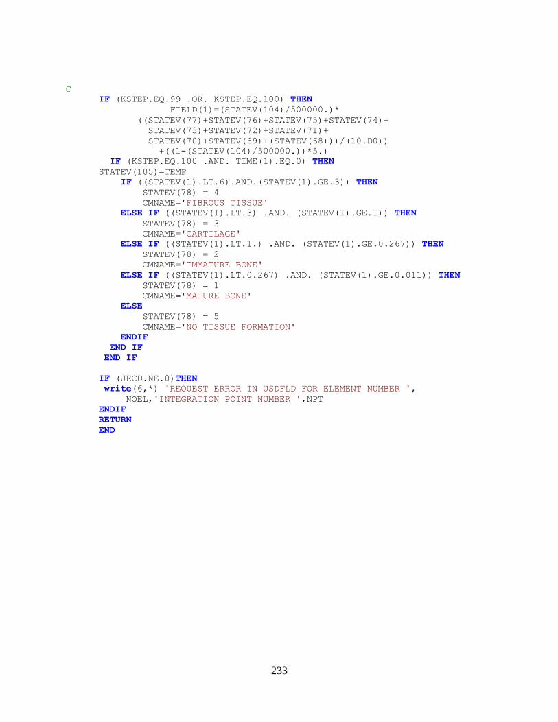
233

C

IF (KSTEP.EQ.99 .OR. KSTEP.EQ.100) THEN

FIELD(1)=(STATEV(104)/500000.)*

1 ((STATEV(77)+STATEV(76)+STATEV(75)+STATEV(74)+

2 STATEV(73)+STATEV(72)+STATEV(71)+

3 STATEV(70)+STATEV(69)+(STATEV(68)))/(10.D0))

4 +((1-(STATEV(104)/500000.))*5.)


STATEV(105)=TEMP


STATEV(78) = 4



STATEV(78) = 3

CMNAME='CARTILAGE'


STATEV(78) = 2



STATEV(78) = 1


ELSE

STATEV(78) = 5


ENDIF

END IF

END IF

IF (JRCD.NE.0)THEN

write(6,*) 'REQUEST ERROR IN USDFLD FOR ELEMENT NUMBER ',

1 NOEL,'INTEGRATION POINT NUMBER ',NPT

ENDIF

RETURN

END

computational simulation of fracture repair in stem cell

Documents