Comprehensive review of structural deterioration ofwater mains: physically based models

Rajani, B.B.; Kleiner, Y.

A version of this paper is published in / Une version de ce document se trouve dans:Urban Water, v. 3, no. 3, Oct. 2001, pp. 151-164

www.nrc.ca/irc/ircpubs

NRCC-43722

1

Comprehensive Review of Structural Deteriorationof Water Mains: Physically Based Models

B. Rajani and Y. Kleiner

Abstract: This paper provides a comprehensive (although not exhaustive) overview of the

physical/mechanical models that have been developed to improve the understanding of the

structural performance of water mains. Several components have to be considered in modelling

this structural behaviour. The residual structural capacity of water mains is affected by material

deterioration due to environmental and operational conditions as well as quality of

manufacturing and installation. This residual structural capacity is subjected to external and

internal loads exerted by the soil pressure, traffic loading, frost loads, operational pressure and

third party interference. Some models address only one or a few of the numerous components of

the physical process that lead to breakage, while others attempt to take a more comprehensive

approach. Initial efforts were aimed mainly towards development of deterministic models, while

more recent models use a probabilistic approach to deal with uncertainties in defining the

deterioration and failure processes. The physical/mechanical models were classified into two

classes: deterministic and probabilistic models. The effect of temperature on pipe breakage is

discussed from three angles; the first deals with temperature effects on pipe-soil interaction, the

second deals with frost load effects and the third provides a brief review of various attempts to

statistically quantify influence of temperature on water main failure.

This paper complements the companion paper “Comprehensive Review of Structural

Deterioration of water mains: Statistical Models”, which reviews statistical methods that explain,

quantify and predict pipe breakage or structural failures of water mains.

Key words: water main failure, physically based models, deterministic, probabilistic, frost

load, structural deterioration, temperature effects.

2

Introduction

The physical mechanisms that lead to pipe breakage are often very complex and not

completely understood. These physical mechanisms involve three principal aspects: (a) pipe

structural properties, material type, pipe-soil interaction, and quality of installation, (b) internal

loads due to operational pressure and external loads due to soil overburden, traffic loads, frost

loads and third party interference, and (c) material deterioration due largely to the external and

internal chemical, bio-chemical and electro-chemical environment. The structural behaviour of

buried pipes is fairly well understood except for issues like frost loads and how material

deterioration affects structural behaviour and performance. Consequently, extensive efforts have

been applied to model the physical processes of the degradation and failure of buried pipes.

As discussed in the companion paper, more than two thirds of all existing water pipes are

metallic (about 48% cast iron and 19% ductile iron). From the 1880s to the early 1930s grey cast

iron pipes were manufactured by pouring molten cast iron in upright sand moulds placed in a pit.

These pipes were known as pit cast iron. In 1920s/1930s a new manufacturing process was

introduced in which pipes were horizontally cast in moulds made of sand or metal that spun as

the moulds were cooled externally with water. These pipes were known as spun cast iron, which

had better material uniformity than their predecessors, with corresponding improvements in

material properties. In 1948 the composition of the iron was changed to produce what is known

as ductile iron pipe, which was more ductile and less prone to graphitisation. However, industrial

production of ductile iron pipe did not begin until the late 1960s. By 1982 virtually all new iron

pipes were ductile iron.

The predominant deterioration mechanism on the exterior of cast and ductile pipes is electro-

chemical corrosion with the damage occurring in the form of corrosion pits. The damage to grey

cast iron is often disguised by the presence of “graphitisation”. Graphitisation is a term used to

describe the network of graphite flakes that remain behind after the iron in the pipe has been

leached away by corrosion. Either form of metal loss represents a corrosion pit that will grow

with time and eventually lead to a water main break. The physical environment of the pipe has a

significant impact on the deterioration rate. Factors that accelerate corrosion of metallic pipes are

stray electrical currents, soil characteristics such as moisture content, chemical and

microbiological content, electrical resistivity, aeration, redox potential, etc. The interior of a

3

metal pipe may be subject to tuberculation, erosion and crevice corrosion resulting in a reduced

effective inside diameter, as well as a breeding ground for bacteria. Severe internal corrosion

may also impact pipe structural deterioration. The supply water affects the internal corrosion in

pipes through its chemical properties, e.g., pH, dissolved oxygen, free chlorine residual,

alkalinity, etc., as well as temperature and microbiological activity.

The long-term deterioration mechanisms in PVC pipes are not as well documented mainly

because these mechanisms are typically slower than in metallic pipes and also because PVC

pipes have been used commercially only in the last 35 to 40 years. These deterioration

mechanisms may however include chemical and mechanical degradation, oxidation and

biodegradation of plasticisers and solvents (Dorn et al. 1996).

Asbestos-cement and concrete pipes are subject to deterioration due to various chemical

processes that either leach out the cement material or penetrate the concrete to form products that

weaken the cement matrix. Presence of inorganic or organic acids, alkalis or sulphates in the soil

is directly responsible for concrete corrosion. In reinforced and pre-stressed concrete, low pH

values in the soil may lower the pH of the cement mortar to a point where corrosion of the pre-

stressing or reinforcing wire will occur, resulting in substantial weakening of the pipe (Dorn et

al. 1996).

Pipe breakage is likely to occur when the environmental and operational stresses act upon

pipes whose structural integrity has been compromised by corrosion, degradation, inadequate

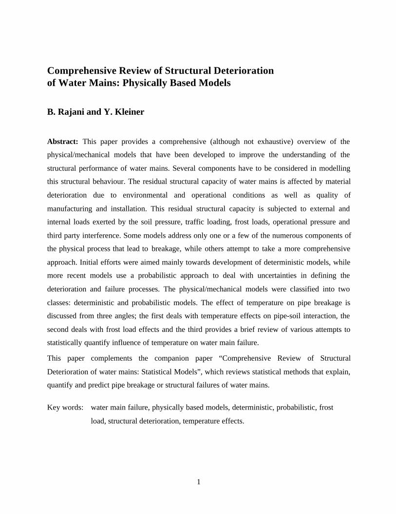
installation or manufacturing defects. Pipe breakage types were classified by O’Day et al. (1986)

into three categories: (1) Circumferential breaks, caused by longitudinal stresses; (2) longitudinal

breaks, caused by transverse stresses (hoop stress); and (3) split bell, caused by transverse

stresses on the pipe joint. This classification may be complemented by an additional breakage

type i.e., holes due to corrosion. Circumferential breaks due to longitudinal stress are typically

the result of one or more of the following occurrences: (1) thermal contraction (due to low

temperature of the water in the pipe and the pipe surroundings) acting on a restrained pipe, (2)

bending stress (beam failure) due to soil differential movement (especially clayey soils) or large

voids in the bedding near the pipe (resulting from leaks), (3) inadequate trench and bedding

practices, and (4) third party interference (e.g., accidental breaks, etc.). The contribution of

internal pressure in the pipe to longitudinal stress, although small, may increase the risk of

4

circumferential breaks when occurring simultaneously with one or more of the other sources of

stress.

Longitudinal breaks due to transverse stresses are typically the result of one or more of the

following factors: (1) hoop stress due to pressure in the pipe, (2) ring stress due to soil cover

load, (3) ring stress due to live loads caused by traffic, and (4) increase in ring loads when

penetrating frost causes the expansion of frozen moisture in the ground.

This paper reviews physical/mechanical models that lead to an improved understanding of

structural performance or behaviour of buried watermains. It complements the companion paper

(Kleiner and Rajani 1999), which provides a critical review of the statistical models that attempt

to explain, quantify and predict pipe breakage. The two papers share the same format, which

provides a description, critique and data requirements for each model. The reader can thus

readily identify the principal characteristics of the models with the corresponding limitations and

data requirements. Some equations are provided for each models as an illustration of their

complexity (or simplicity) and the type of data that is required for their application.

Physical/mechanical Methods

The traditional design of buried pipes has been based on physical behaviour that attempts to

provide pipe resistance capacity against expected loads (operational and environmental) with a

sufficient margin of safety. The prediction of the mechanical performance of buried pipes with

material deterioration requires understanding of several components as is graphically illustrated

in Figures 1 and 2. The mechanical behaviour of most of these components is fairly well

established and information is available through standards or textbooks (e.g., Young and Trott

1984; Moser 1990) except for recent developments. Therefore, components such as calculation

of stresses on pipes subjected to earth and traffic loads are not discussed in detail here. The

review is divided into four sections. The first provides a description of some recent work that has

been done to model individual components from the array of loadings and degradation

mechanisms that act on the pipe. The second and the third sections describe more general models

that attempt to capture simultaneously several components. The second and third sections deal

with deterministic and probabilistic models, respectively. Efforts to relate pipe breakage rates to

temperature effects on a statistical and physical basis are reviewed in the fourth section. The

statistically based models are not breakage prediction models in the strict sense since

5

temperatures cannot be predicted in the long-term but do provide an insight into how

temperatures have been observed to affect water main breakage rates.

Figure 1. Failure modes for buried pipes: direction tension (top left), bending or flexuralfailure (middle) and hoop stress (bottom).

6

Figure 2. Conditions leading to corrosion.

Differential aeration

7

Individual Components of Physically Based Models

Frost load

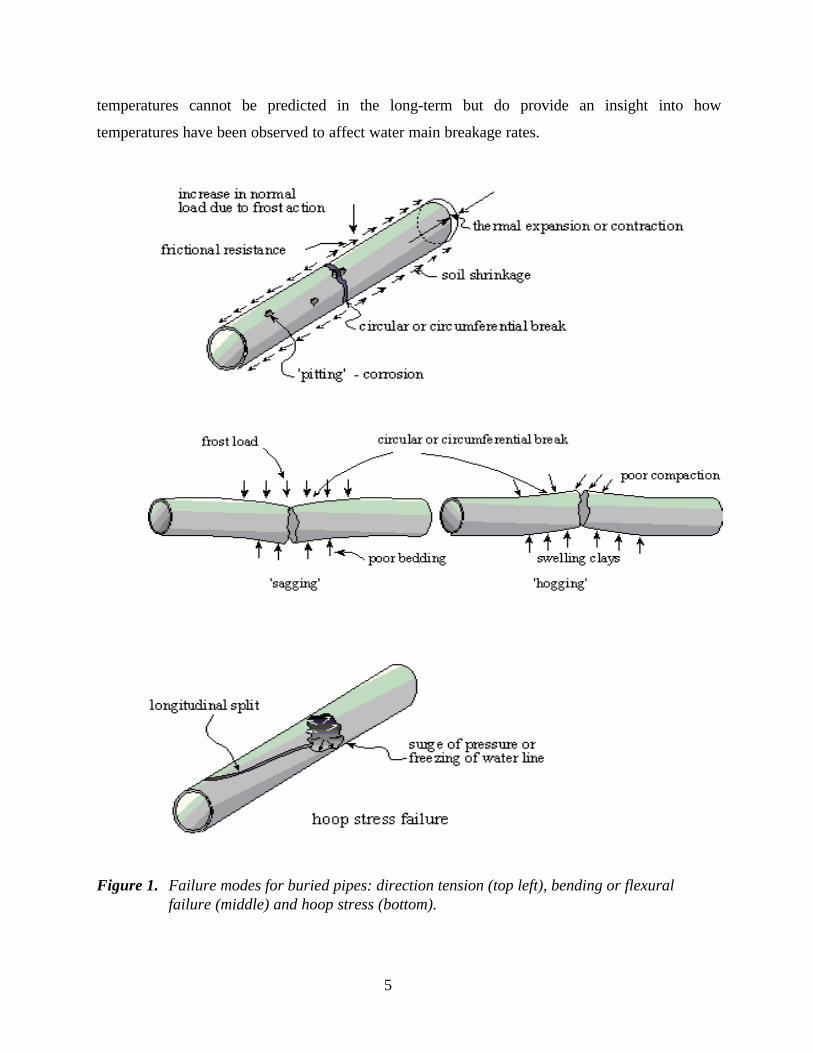
Model description. The high breakage frequency of water mains during winter has been

attributed to increased earth loads exerted on the buried pipes, i.e., frost loads. The mechanics

and circumstance that lead to the generation of frost load remained unexplained except by

heuristic arguments. Rajani and Zhan (1996) and Zhan and Rajani (1997) presented methods to

estimate frost load on buried pipes in trenches and under roadways, respectively. The frost load

in a typical trench was calculated from

ph

KB

k d

H s d Bfi

tip

d

s fi

i o

N

fi

d

T

s =

+LNMM

OQPP

-=å

β

1,d i

(1)

where ps = frost load at any point s, df = frost depth, i = time step number, NT = number of time

steps, hf = total frost heave, Bd = trench width, Ktip = stiffness of elastic half-space of unfrozen

soil mass below freezing front, β = attenuation factor, ks = backfill-sidewall shear stiffness, H =

Boussinesq function to determine the influence of stress, s = location below surface where frost

load is calculated.

In a trench, the frost load develops primarily as a consequence of different frost

susceptibilities of the backfill and the sidewalls of the trench and the interaction at the trench

backfill-sidewall interface. Trench width, differences in frost susceptibilities of backfill and

trench sidewall materials, stiffness of the medium below the freezing front and shear stiffness at

backfill-sidewall interface play important roles in the generation of frost loads. Thus, it is

preferable to use a backfill material that has a matching or lower frost susceptibility than that of

the sidewall in order to mitigate against the development of excessive frost loads.

Critique. The frost load models improve the understanding of the mechanisms that lead to

the development of frost loads and thus enable the development of mitigating measures. The

models are complex and some of the input parameters are not readily available. Although the

models have been validated with field measurements, further validations are required to gain

confidence in their use. The current field validation data indicate that frost loads could develop to

magnitudes of up to twice the geostatic or gravity earth loads.

8

Data requirements. The models require data such as continuous freezing index, soil backfill

properties such as porosity, segregation potential, unfrozen water content and thermal gradient at

the freezing front, frost depth and other related variables to predict the frost load on a pipe buried

at a particular depth. The segregation potential of backfill is a frost heave property that is

conceptually similar to hydraulic conductivity and is not commonly used in civil engineering

practice except by specialists in cold regions engineering. The estimates of thermal gradients at

the freezing front are dependent on material properties as well as thermal boundary conditions

which makes it necessary to use finite element analysis to solve practical trench configurations.

The frost load models give frost load as a function of time but only the maximum frost load may

be required for most design or structural evaluation procedures.

Pipe-soil interaction analysis

Model description. The interaction of pipe-soil needs to be considered in the in-plane and

longitudinal directions. Spangler (1941) developed an understanding on the interaction of in-

plane behaviour of flexible pipes with surrounding soils. Watkins and Spangler (1958) improved

on the formulation to include the modulus of soil reaction, a property that can be measured. The

total circumferential stresses were subsequently obtained by adding the stresses that result from

internal pressure, ring compression due to external loads and stress due to ring deflection

resulting from static and dynamic loads (e.g., earth pressure, traffic, etc.). The total in-plane

stress σθ was calculated as

σ γ σθ = ++

+FHG

IKJ+

Prt

k E trE t k Pr

C BI C F

Ai m p

p d id d

c tf

6243 3

2 (2)

where Cd, Ct = earth and surface load coefficients, km = bending moment coefficient, Ep = pipe

elastic modulus, Pi = internal pressure, r and t = mean pipe radius and wall thickness, kd =

deflection coefficient dependent on the distribution of vertical load and reaction, Ic = vehicle

impact factor, F = wheel load on surface, σf = stress due to pipe ring deflection, Bd = trench

width, γ = soil backfill unit weight, A = effective length of pipe.

Rajani et al. (1996) developed a pipe-soil interaction analytical model for the longitudinal

response of jointed water mains to changes in internal and external pressures and temperature

changes. The response in terms of axial s x and hoop s ? stresses was expressed as

9

σ χ χ χ αx p i p pEux

P E T=∂∂

+ −1 2 3 ∆ (3)

σ ν κθ =P Dt

h D t E E kip s p s( , , , , ) (4)

where Ep = pipe elastic modulus, u and, x = axial displacement in longitudinal direction x, νp =

pipe Poisson ratio, αp = coefficient of pipe thermal linear expansion, Pi = internal pressure, ∆T =

temperature differential, Es = elastic soil modulus, D, t = pipe diameter and wall thickness, ks =

pipe-soil reaction modulus, χ1, χ2, χ3, κ = constants as function of soil and pipe properties.

The model for longitudinal response permitted sensitivity analysis to identify key variables

that play a major role in the overall behaviour of buried water mains. A sensitivity analysis of

ductile iron and PVC water mains indicated that maximum axial stress increased substantially

with a decrease in pipe size. This model provided a credible explanation to the observation (e.g.,

Kettler and Goulter 1985) that under a given set of conditions, small diameter water mains had a

higher incidence of breaks per unit length, compared to larger diameter pipes. The model showed

that cold ground temperatures can lead to an increase in circular water main breaks and the

additional stresses imposed on corroded water mains can be particularly damaging. This model

provided a physical explanation to the observations of increased pipe breakage at cold

temperatures that were reported by others as discussed later in this paper. The frozen soils or

backfill surrounding the buried pipe have a positive restraining effect and thus contribute

towards the reduction of hoop stress. Kuraoka et al. (1996) validated the model developed by

Rajani et al. (1996) by analysing field data collected on instrumented PVC water mains in

Edmonton, Canada.

Critique. The Spangler-Watkins in-plane pipe-soil interaction model assumed that the

primary load-resistance action only takes place in the vertical direction, in the plane that is

perpendicular to the longitudinal direction of the pipe. This in-plane consideration for the load-

resistance action is appropriate for moderate to large diameter pipes and inadequate for small

diameter pipes. Moreover, the influence of ground and water temperature was not considered in

the Spangler-Watkins model. The longitudinal model developed by Rajani et al (1996) accounted

for temperature differentials and explained the frequently observed occurrences of

circumferential breaks in small diameter mains. However, none of these models considered the

stresses imposed on the mains during extreme dry seasons as a consequence of soil shrinkage.

10

These pipe-soil interaction models are useful to explain observed behaviour of pipe segments

without any degradation such as corrosion pits, thus they cannot, in themselves, be used to

predict how the number of water main breaks will vary with time.

Data requirements. The data required by these models are readily available except for the

elastic soil reaction modulus and the pipe-soil reaction modulus. The seasonal ground and water

temperatures are necessary to determine the influence they exert on the behaviour of the pipe

under expected temperature variations. It is also possible to use ambient air temperatures as

surrogate variables wherever precise water and ground temperature data are unavailable.

Residual structural resistance

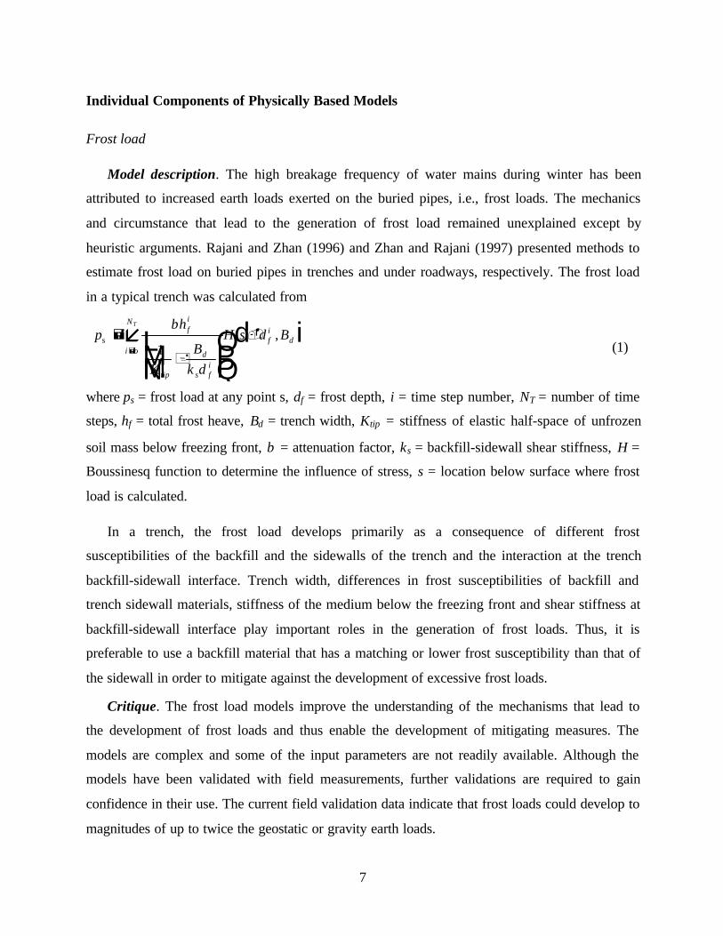
Model description. The assessment of corrosion pits on the structural resistance of thin-

walled steel pipes is typically done through the application of ASME/ANSI B31G (1991). This

approach was developed semi-empirically, based on experiments where corroded steel pipes

were tested to failure. Later, Kiefner and Vieth (1989) conducted additional tests and developed

an analytical failure model to predict the pressure at which a pipe with a corrosion pit would fail

( )

−

−=

o

oy

MAAAA

r

hsldp

11

),(0 (5)

where p0 = pressure in the pipe at failure , d = maximum depth of corrosion defect, A = cross-

sectional area of metal lost in the corroded region projected onto the longitudinal axis of the

pipe, Ao = the original cross sectional area of the corroded region, l = maximum total length of

corrosion defect, r = pipe radius, h = pipe wall thickness, sy = pipe yield strength, M = Folias

factor that accounts for the bulging of the pipe before failure when subjected to internal pressure.

Critique. This model to assess the reduction in structural resistance in the presence of

corrosion pits was developed for ductile materials such as steel pipes that are used primarily in

the oil and gas industry. The bulging in the pipe prior to failure (accounted for by the Folias

factor) is a phenomenon that is typical to ductile materials only. Since the model has not been

validated with pipe materials other than steel, it is not clear whether it is appropriate for cast iron

or even ductile iron pipes. The model was developed to represent the bursting failure mode,

which in turn corresponds to the longitudinal breaks.

The model requires three-dimensional characteristics of corrosion pits in the pipe. This

information for oil and gas pipelines is readily obtainable by using tools known as pigs. The use

11

of these pigs in oil and gas pipelines is increasing because the high cost of failure make their

application in frequent inspections economically viable. In the water supply industry similar pigs

have recently been developed but they are still in their early stage and are relatively expensive to

use. Consequently, it seems that frequent inspections with pigs may currently be warranted only

for large transmission mains. It is also possible that as the usage of these pigs increases, the cost

will decrease, enabling more frequent inspection cycles.

Data requirements. The data required includes the material properties and condition

assessment of a pipe to determine the three-dimensional characteristics of its corrosion pits.

Considerable progress has recently been made on practical non-destructive condition assessment

techniques to inspect pipe which should facilitate the use of these types of models to assess the

longevity of the inspected pipe.

Model description. Rajani et al. (1999) have recently completed an experimental study where

coupons of pit and spun cast iron pipe samples with and without corrosion pits were tested.

Results from mechanical tests were used to establish how dimensions and geometry of corrosion

pits influence the residual strength of gray cast iron mains. The test coupons had corrosion pits

with “small” areas in relation to the coupon size. The authors suggested that the nominal tensile

stress (σ n) at which fracture took place depended on the material and corrosion pit dimensions as

given by

σα

βn

q

n

s

K

d t a= b g (6)

where β = geometric factor dependent on the dimensions and shape of the corrosion pit, an =

lateral dimension of corrosion pit size, Kq = provisional fracture toughness, d = pit depth, α, s =

constants obtained from experimental tests, t = pipe wall thickness. The above expression is

essentially the same as the basic fracture mechanics equation that relates stress, defect size and

geometry through the stress intensity or toughness of the material.

Critique. The model is based on small-scale laboratory tests and it needs to be validated with

large-scale tests. The model also makes use of fracture toughness, a material property that is not

readily available for pipe materials of interest. The experimental work was carried out only on

brittle material such as cast iron, which is distinct from the work reported by Keifner and Veith

(1989) on ductile steels.

12

Data requirements. The data input requirements are similar to those required in the model

suggested by Keifner and Veith (1989).

Corrosion status index

Model description. Kumar et al. (1984) proposed a corrosion status index (CSI) to

characterise the condition of cast and ductile iron mains. Although CSI was originally developed

for gas mains it also found support (with some modifications) in the water distribution field. The

CSI is given by

tP

CSI av100100 −= (7)

where Pav = average corrosion pit depth of a 1 m section of pipe, t = pipe wall thickness.

While the CSI of a new pipe is 100, a pipe with average corrosion pit depth of 70% of the

original wall thickness will have a CSI of 30. The authors report an empirical observation that

the ratio between the average and the maximum corrosion pit depth in a pipe equals 0.7. Further,

they reported that the average corrosion pit depth is almost independent of the length or the

location of the pipe segment that is examined. Thus, full penetration of the pipe wall would occur

for a CSI of 30. The authors then reported formulating “lookup tables” for predicting CSI while

considering pipe coating, soil pH and resistivity, age of leak, rate of pit growth, presence of

sulphides in the soil and effects of moisture. Although they provided only scant information, it

appears that they used a simple power model of the form D = atn (D is the pit depth, a is a

proportion constant, t = time) to predict the basic corrosion rate, where a was modified by other

constants representing the effects of the various factors mentioned above. Once a CSI of 30 was

reached, a first leak was assumed to have occurred. Kumar et al. (1984) developed a procedure to

predict the number of breaks over time, given that the first break has occurred. Their model was

based on an exponential increase of breaks over time but they provided very little information as

to how they had considered all the factors in this prediction model. A software package “Piper”

was subsequently developed for planning and management of pipelines based on these models.

Critique. This model could be also classified as a statistical time-exponential model, as it

involves corrosion modelling for predicting the time to the first break, and what appears to be a

statistical model to predict subsequent breaks. Kumar et al. (1984) provided few details about

their model but the following observations can be made based on the limited available

13

information. Their power model to predict corrosion rate appears to be similar to Rossum’s

(1969), although no reference was provided. In general the power model requires further

validation as discussed in more detail later. Further, the value for the exponent n used is 0.58,

which seems high compared to values (0.17 to 0.5) used in the literature (e.g., Rossum 1969).

The exponential increase of breaks over time given that a first break has occurred is similar to

the model proposed by Clark et al. (1982). A few examples provided by the authors in the report

indicate that the breakage rate (subsequent to the first break) increases extremely rapidly. No

information is provided on any validation or even “goodness of fit” that would be associated

with their predicted versus observed values.

Data requirements. It appears that the data that are required include pipe age, type - wall

thickness, diameter, joints soil properties – resistivity, chlorides, sulphides, pH, moisture, and

year of first leak (if available).

Physical Deterministic Models

Model description. Doleac (1979) and Doleac et al. (1980) used the power function proposed

by Rossum (1968) to relate corrosion pit depth with the pipe age to predict the remaining wall

thickness of pit cast mains.

p K K pH t An an n n a= − −10b gρ (8)

where p = average pit depth, a, Kn, Ka = empirical constants derived from field or lab tests, Aa =

pipe surface area exposed to corrosion, pH = soil pH, ρ = soil resistivity, n = soil aeration

constant, t = time (years).

The parameter constants were also taken from Rossum (1968). The authors extracted five

pipe samples, and their surrounding soil properties in Vancouver, Canada and measured their

maximum and average pit depths. Comparison of the maximum and mean pit depth observed to

the corresponding values calculated1 from equation (8) yielded mixed results. Then they

substituted the remaining average wall thickness into Barlow’s equation of pipe hoop stress

tpD

S2

= (9)

1 The pipe surface area was not included in these calculations.

14

where p = internal pressure, D = outside pipe diameter, S = hoop stress on the pipe, t = pipe wall

thickness. Pipe failure was defined as “a reduction in pipe wall thickness to a point where a

pressure surge in the pipe, equal to 50% of the working pressure, would raise S to the material’s

elastic limit”.

Critique. The model proposed by Doleac (1979) and Doleac et al. (1980) has some

shortcomings. There have not been many documented studies that validate Rossum’s (1968)

power function to predict the growth of corrosion pit depths with time. Doleac’s five-sample test

is not sufficient to provide significant validation, especially in light of their seemingly mixed

results. An attempt to re-create some of the results presented by Doleac (1979) for this review

was difficult due to lack of information on values used for some of the parameters in the model.

Further, the parameter A (exposed surface area) in equation (8) was used by Rossum (1968) to

translate maximum pit depth into average pit depth in a pipe. It is not clear what exposed area

should be considered for a given length of pipe, and how an uncoated pipe should be considered.

This difficulty may have been the reason why Doleac did not consider parameter A at all in the

model. Another limitation is that the structural pipe capacity is based solely on pressure

requirements and does not adhere to all the requirements of the standards (AWWA/ANSI C101-

67 (R1977)) in existence when these mains were first installed, e.g., external loads, etc.

Data requirements. The data that are required for this model are pipe age and surrounding

soil properties, such as resistivity, pH and aeration constant, which can be obtained relatively

easily and economically. The exposed surface area of the pipe needs clarification and how it

should be calculated or estimated in practice.

Model description. Randall-Smith et al. (1992) proposed a linear model based on an

assumption that corrosion pit depth has a constant growth rate (often referred to as corrosion

rate), to estimate remaining service or residual life of water mains.

ρ δ=+

FHG

IKJ−

tP P

te i

(10)

where ρ = remaining life, t = age of water main, δ = thickness of original pipe wall, Pe = external

pit depth, Pi = internal pit depth.

The model was developed as a rough screening tool to identify potential problems rather than

provide a means to predict a break. It was argued that since all the calculations were based on the

15

most pessimistic assumptions, a result indicating remaining life that exceeded the planning

horizon meant that failures from corrosion pitting were unlikely to occur within the planning

period. Conversely, if the calculated remaining life was shorter than the planning period, this

would indicate that it might be necessary to do rigorous analysis. It was recommended that mean

or median corrosion pit depths should be used in the equation (10) for grey cast iron mains, while

maximum pit depths should be used for ductile iron mains. This recommendation followed from

the recognition that grey iron mains fail as a consequence of the brittle nature of the materials

and ductile iron mains fail by developing “pin holes”.

Critique. The assumption of a constant corrosion rate over the life of the pipe is questionable.

The assumption about the external and internal corrosion pits coincide at the same location is

highly unlikely because the conditions and mechanisms that promote internal and external

corrosion are different and independent. This assumption leads to very conservative estimates for

the remaining service life of water mains, which indeed was the intention of the authors.

However, the model assumes failure when the sum of the internal and external corrosion pit

depth equals wall thickness. This assumption considers neither stresses acting on the pipe nor its

stress resisting capacity. Since the structural integrity of the pipe can be breached without full

perforation of its wall, the model may not be as conservative as it may seem, thus it may not

even be suitable for a crude screening. Further, the model expresses the remaining service life as

a multiple of the current pipe age, which is neither intuitive nor useful.

Data requirements. The model requires the pipe age, wall thickness and depths of internal

and external corrosion pits obtained during the condition assessment of the pipe. The exhumation

of many pipe samples may not be economical to measure corrosion pit depths. As previously

noted, progress on practical non-destructive condition assessment techniques may soon

encourage measurements of corrosion pit depth on a routine basis.

Model description. Rajani and Makar (1999) described a methodology to estimate the

remaining service life of grey cast iron mains by considering changes in the structural resistance

of a pipe as a result of corrosion pits. They defined the “time of death” of an individual pipe

segment as the time at which its mechanical factor of safety fell below a minimum acceptable

value set by the utility owner. They calculated the residual resistance of grey cast iron mains

based on corrosion pit measurements while explicitly considering anticipated corrosion rates.

The calculations combined elements from equations (1), (3), (4), (6), (8) and (9). Direct

16

inspection or non-destructive evaluation technology could be used to measure corrosion pits. The

methodology comprised all the major components identified in Figure 3 that should ideally be

included in a physical deterministic model. The methodology used a re-iterative procedure to

estimate the remaining service life of segments of grey cast iron pipe. The block diagram in

Figure 4 illustrates the procedure.

The proposed methodology determined base conditions using pipe information (diameter,

wall thickness, date of installation, depth of burial, pipe type – spun or cast); soil condition (type,

pH, density, resistivity, aeration quality); installation information (laying condition, load factor,

coefficient of horizontal stress at rest, coefficient of sliding friction); operational conditions

(water pressure, surge pressures, summer and winter air and water temperatures, wheel loads,

vehicle impact factor, frost load factor).

The water utility needs to choose a value for the minimum factor of safety for each pipe

segment in its system as part of the initial decision making process. A factor of safety of one

signified imminent failure, whereas a factor of safety greater than one, say 1.2, might provide

leeway to repair or replace pipe segments before failure occurred.

The methodology proposed two feasible approaches to determine corrosion pit characteristics

of grey cast iron mains, an indirect approach using measurements taken by non-destructive

evaluation (NDE) technology, or a direct approach where corrosion pit measurements are

performed on exhumed pipe samples.

The typical lack of historical corrosion rate data prompted the authors to propose two options

to estimate the remaining service life of grey cast iron water mains. The “one-time pit

measurement” option provided an estimate based on the initial pipe condition and one more

corrosion pit measurement. These two points would then be used in a Rossum-like (1968) power

model to approximate the prevalent corrosion rate. The “multiple-time pit measurement” option

can provide a more refined estimate of the remaining service life by basing the corrosion rate

estimates on a more extensive set of data. The choice between the options would depend on

when the methodology is first applied and on the number of pit measurements available. The

dimensions of each significant corrosion pit or its expected growth rate is combined to calculate

the residual tensile strength. The time required for the factor of safety of the pipe segment to fall

below the target value set by the utility is calculated iteratively.

17

Figure 3. Physical/mechanical models.

Pipe residualstructuralresistance

External loads

Pipe characteristics

Environmental andoperationalconditions

Corrosion pit measurements:Direct (sampling) or indirect(NDE)

Corrosionmodel

Remainingservice life

Designcriteria

Optimalinspectionschedule

Earth loads (Marston-Spangler)Frost load (Rajani & Zhan)Traffic loads (Hall & Newmark) Soil-structure

interactionanalysis

In-plane (Spangler-Watkins)Longitudinal (Rajani et al.)

Hydrostatic pressuresSurge (cyclic) pressuresAir, water and ground temperaturesSoil properties

1

210

9

87

65

4

3

Rossum

Kiefner & ViethRajani & Makar

18

Figure 4. Physical deterministic model proposed by Rajani and Makar (2000).

residual pipestructural resistance

design loads

pipecharacteristics

environmentalconditions

designcriteria

iterate over wallthickness

pipe wallthickness factor of

safety

corrosion pit measurements:direct (sampling) or indirect

methodologyoption

“one-time”

corrosion model

“multiple-time”

iterate overtime

remainingservice life

corrosion pit measurements:indirect (NDE)

comparestress-states

new designpipe

evaluation

factor ofsafety

designcriteria

designcriteria

residual pipe structuralresistance

remainingservice life

19

Critique. The methodology proposed by Rajani and Makar (1999) relies on the measurement

of corrosion pits by direct inspection or indirectly through the use of non-destructive techniques.

The opportunity to directly measure corrosion pits may not always be available because of

economic or operational conditions, whereas NDE techniques are currently not developed

enough to provide accurate geometry of corrosion pits. The methodology is similar in concept to

the physical probabilistic models developed for oil and gas pipelines discussed later except that

all the input and output are in deterministic terms. Rajani and Makar (1999) point out the

uncertainties in estimating corrosion rates, and the significant impact of these uncertainties on

the prediction of the remaining service life of water mains. This conclusion is in line with the

conclusion reached by Ahammed and Melchers (1994) in the development of the physical

probabilistic model described later. The methodology needs to be validated and possible

improvements could incorporate some probabilistic formulations to explicitly account for the

uncertainties inherent in the data.

Data requirements. A variety of background data are necessary to define the base condition.

The model requires the material properties, current pipe age, wall thickness and internal and

external corrosion pits depths to estimate the remaining service life of each pipe or pipe section.

The specific material properties required are tensile strength, fracture toughness, elastic modulus

and flexural strength. The exhumation of many pipe samples may not be an economical option to

measure corrosion pits depths in small distribution pipes. Progress on practical non-destructive

evaluation techniques should encourage depth measurements of corrosion pits on a routine basis.

Physical Probabilistic Models

Model description. Ahammed and Melchers (1994) described a model to estimate the

probability of failure in steel pipelines. In their model they used equation (2) of the Spangler-

Watkins in-plane pipe-soil interaction model as their underlying mechanical stress model2. For

the wall thickness variable in equation (2) they used a simple power function, D = ktn, where D

is the loss of wall thickness at time t, and k and n are regression parameters. Thus they obtained

an equation that related the in-plane tensile stress to the age of the pipe. Each parameter and

independent variable in the model was then assumed to have a probability distribution with a

2 The stress due to pipe ring deflection component was not considered by Ahammed andMelchers (1994).

20

known mean and variance. A second-moment description method was then used to approximate

the mean and variance of the dependent variable, namely the in-plane tensile stress.

Subsequently, the reliability index of the pipe was derived, and the contribution of each

parameter to the uncertainty (or the variance) of the total reliability could be evaluated. A

sensitivity analysis indicated that remaining service life was influenced primarily by the

parameters involved in the power function for corrosion estimates. This influence was on both

the magnitude (mean) of the reliability and on the uncertainty of the reliability. In a subsequent

publication, Ahammed and Melchers (1995) extended this model to include leakage of fluids

through corrosion pits. Leakage in pipelines was modelled as an exponential function of time and

corrosion pitting rate. The failure associated with leakage was that which exceeded a pre-defined

limit.

Critique. The models developed by Ahammed and Melchers (1994, 1995) fall within the

probabilistic framework of previously developed mechanical models. This probabilistic approach

provides insight into the contribution of each parameter to the uncertainty of the results, which is

ignored in the deterministic models. There may be some concern with the fact that the second-

moment description method, when used with a first-order approximation, is suitable mainly for

reliability functions that are relatively linear about the point of failure. This may not always be

the case as it may depend on the value of the exponent of the power function. The model in itself

suffers from the limitations listed previously for the Spangler-Watkins in-plane pipe-soil

interaction model, and the power function as a model for corrosion rate. These limitations

include the exclusion of pipes made of brittle material, consideration of stresses only in the

circumferential direction (in-plane analysis) and not longitudinal, and the difficulty in deriving

the parameters for the corrosion power function. Further, this model does not consider the stress

due to pipe ring deflection, which may sometimes be significant. The proposed leakage failure

criterion may be practical for the oil and gas industry, where flows are tightly monitored and

controlled. In the water industry this criterion seems unrealistic especially in North America,

where rigorous water metering is currently practised by few water utilities.

Data requirements. The data required are similar to those required for the Spangler-Watkins

in-plane pipe-soil interaction model, plus the parameters for the corrosion power function. The

mean values as well as variances (or standard deviations) are required for all data. Most of these

properties are readily available except for corrosion parameters in the power function described

21

earlier. Since the model is most sensitive to corrosion parameters, it is paramount to obtain

reliable corrosion parameters and that may not always be easy to do in practice. If the actual or

approximate probability density functions of these parameters were known, it would be possible

to perform Monte-Carlo simulation and obtain results that are more accurate. The Monte-Carlo

simulation would also give an idea of how much precision is sacrificed in using the second

moment approximation method.

Model description. Several probabilistic physically based models, e.g., Hong (1997, 1998),

Jones (1997a, 1997b), Linkens et al. (1998), Pandey (1998), Stephens (1994a, 1994b), have been

proposed, that use the residual strength of pipelines suggested by Keifner and Vieth (1989). Two

of these models developed for the condition assessment of oil and gas pipelines are discussed

briefly here.

Pandey (1997) presented a general probabilistic framework to estimate reliability by

incorporating the impact of inspection and repair activities planned over the service life of a

pipeline vulnerable to corrosion. The intent of this model was to schedule the optimal inspection

interval and repair strategy while maintaining adequate reliability throughout the service life of

the pipeline.

Hong (1997) suggested that the ratio between the true (observed) remaining pipe strength and

the predicted value p0(d,l) (equation 5) is a random variable Cm that is approximately log-

normally distributed. Hong (1998) developed a probabilistic expression for the load resistance

ratio, which is the ratio between the operating pressure acting on the pipe and the pipe remaining

strength under pressure. This probabilistic expression comprised the probability distributions of

Cm as well as the corrosion pit dimensions d and l. He then proposed a Markov process in which

initial state of the pipe was determined following a non-destructive inspection procedure. The

deterioration of the load-resistance factor was modelled as a birth process (or Yule process) with

a linear birth rate. The transition probabilities included uncertainties in detecting and accurate

sizing of defects. Optimal inspection schedules were then determined while attempting to

minimise the probabilities of time to failure before inspections and before the end of the pipe

service life.

Critique. These models like those developed by Ahammed and Melchers (1994, 1995) are

suited for ductile pipe materials since they use the description of residual strength suggested by

Keifner and Vieth (1989). Stresses are considered in the in-plane direction only, which is a

22

limitation for broad application to water mains, especially those with smaller diameters.

However, corrosion-pitting rate is not modelled explicitly but the models are posed to take

advantage of periodic inspections of oil and gas pipelines using non-destructive evaluation

techniques. This approach although costly, may be preferable since reliable prediction of growth

of corrosion pits is a significant challenge and involves considerable uncertainties.

Data requirements. The models require the current pipe age, wall thickness and depths of

internal and external corrosion pits, and lengths and their respective probability distributions to

estimate the probability of failure of each pipe or pipe section. As previously noted, active use of

non-destructive techniques to measure corrosion pit depths in the oil and gas industry has

received widespread use because of the economics and existing regulations to meet a specified

level of safety standards.

Model description. UtilNets is a decision-support system for rehabilitation planing and

optimisation of buried grey cast-iron water mains, which is currently being developed under the

sponsorship of the European Union. According to Hadzilacos et al. (2000), the system performs

reliability-based life predictions of the pipes and determines the consequences of maintenance

and neglect over time in order to optimise rehabilitation policy. The system gives a probabilistic

measure of the likelihood of structural, hydraulic, water quality and service failure of pipe

segments and of the entire distribution system. Specific descriptions of the UtilNets model are

not publicly available and hence it is not possible to offer a critique or specific data

requirements. However, based on publications co-authored by the principal developer of the

system, e.g., Camarinopoulos et al. (1996a, 1996b, 1999), the following appears to be relevant to

physical modelling of structural behaviour of pipes.

The authors based their approach on mechanical models similar to those of Rajani and Makar

(1999). They considered factors such as frost load (as a fraction of earth load), earth load, traffic

load, pipe working pressure and surge pressure, temperature change (not clear if ambient or

water temperature), internal and external pipe diameter, bursting strength, tensile strength,

internal and external corrosion coefficients, unsupported length of pipe (causing beam

condition), maximum external load and fracture toughness. They used a simple power function

to model corrosion rates, which is similar to the approach used by Kumar et al. (1984) and

Ahammed and Melchers (1994). They applied these physical/mechanical models in a

probabilistic framework, to compute the reliability of a water main as the probability of its

23

survival over a pre-defined time period. They reportedly developed a computer code in which

they used a combination of Monte-Carlo simulations and approximate quadrature analytical

methods to compute the results numerically. The authors did not provide any information about

the availability of data for the validation of their model.

From the information described above, it appears that the mechanical/physically based model

of UtilNets is close to a probabilistic version of the approach taken by Rajani and Makar (1999),

which is illustrated in Figure 4.

Statistical Treatment of Temperature Effects

The effects of temperature on pipe breakage rates have been observed and reported by many.

Walski and Pelliccia (1982) suggested that pipe breakage rates might be correlated to the

maximum frost penetration in a given year. To account for the lack of frost penetration data, they

correlated annual breakage rates with the air temperature of the coldest month, using a multiple

regression analysis with age and air temperature as the covariatesBTAteetNTtN )(),( 0= (11)

where t = pipe age; N(t0) = breaks per km at year of installation; T = average air temperature in

the coldest month; A, B = constants. The authors did not provide any information as to the

quality of breakage predictions that were obtained by this model.

Newport (1981) analysed circumferential pipe breakage data from various areas of the

Severn-Trent Water Authority. He found that increased breakage rates coincided with cumulative

degrees-frost (usually referred to as freezing index in North America and expressed as degree-

days) in the winter as well as with very dry weather in the summer. He attributed the increase in

winter breakage rates to the increase in earth loads due to frost penetration, i.e., frost loads, and

the summer breakage rates to the increase in shear stress exerted on the pipe by soil shrinkage in

a dry summer. He also observed that when two consecutive cold periods occurred, the breakage

rates (in terms of breaks per degree-frost) in the first one exceeded those of the second one. He

rationalised that the early frost “purged” the system of its weakest pipes, causing the later frost to

encounter a more robust system. Newport (1981) used data from years 1970-1977 to obtain the

following linear relationship (correlation coefficient of 0.9) between the number of water main

breaks and the cumulative degrees-frost in a given year

24

500 frost) of degrees Total(2.5yearper bursts Total += (12)

Equation (12) was derived for the Soar division of the Severn Trent distribution system and

length of water mains was not specified. This linear model suggests that every degree of frost is

responsible for an additional 2.5 breaks but at the same time, only about 50% of the failures may

be explained by cold climate, expressed as cumulative degrees-frost. No model to predict water

main breaks during extreme dry weather was given.

Habibian (1994) analysed the distribution system of Washington (DC) Suburban Sanitary

Commission and observed an increase in water main breakage rate as the temperatures dropped.

He related the breakage rates to the water temperature at the system intake rather than to the

ambient air temperature, reasoning that although their monthly averages are similar, ambient air

temperatures display sharp fluctuations while water temperatures are better surrogates for

underground pipe environment. He concluded that the water temperature drop, rather than the

absolute water temperature, had a determining influence on the pipe breakage rate. He also

observed that in a given winter, similar consecutive temperature drops did not necessarily result

in similar breakage rates, however, typically every time the temperature reached a new low a

surge occurred in the number of pipe breaks. His explanation for this phenomenon concurred

with Newport (1981), namely, that every temperature low “purged” the system of its weakest

pipes, thus a new low affected the pipes that were a little more robust than those that had broken

in the previous cold spell. During the warm seasons the pipes continue to deteriorate and the

process is repeated in the subsequent cold season. It should be noted that Habibian’s (1994)

observations were all based on one-year data. Lochbaum (1993) reported that a study conducted

by Public Service Electric and Gas Co. which showed that the breakage rates of cast iron gas

pipes increased exponentially with the number of degree-days (degree-days were defined as S i? N

[ (65oF-Ti] where Ti is the average temperature in

oF in day i and N is the set of days in a given

month with average temperature below 65oF). Lochbaum (1993) did not present a model relating

the number of water main breaks to monthly degree-days; her observations, however, agreed

with those of Newport (1981) and others. No information is provided as to the causes of pipe

breaks in the warm seasons.

Sacluti et al. (1998) applied an artificial neural network (ANN) to the distribution system of a

sub-division in Edmonton, Canada. The ANN model was applied to the entire network as a

25

single entity (rather than to individual pipes) and was trained with data that included temperature

(water and ambient), rainfall, operating pressure and historical data on break numbers. Since the

model considered an entire network as a single entity, variates such as pipe age, type and

diameter could not be considered, as well as geographical variates such as soil properties. The

network consisted of spun-cast 150-mm (6”) water mains. A sensitivity analysis determined that

rainfall and operating pressure did not contribute to the predictive power of the model were thus

omitted. The authors claim that the model was successfully applied to a holdout sample,

demonstrating that the ANN “learnt” the breakage patterns rather than memorised them3.

The ANN model was applied to a relatively small network with water mains that were

relatively homogeneous with respect to type of pipe and operational and environmental

conditions. A more heterogeneous set of water mains would likely require more data. The model

predicted the number of water main breaks based on a 7-day weather forecast. This requirement

limited its applicability to short term response rather than its use for long term planning

purposes. The uncertainty in the weather forecast models also has a direct influence in the

anticipated short-term response required. In its present form, the model can only be applied to

homogeneous groups of water mains, for short-term planning of the maintenance work force

required during an anticipated cold spell.

The ANN can be a useful tool in predicting water main breaks. Its main strength is that

complex physically based models need not be developed and understood in order to identify

breakage patterns. In that, it is similar to the various probabilistic models. Additional advantages

are that many variates can be easily considered (many variates cause the probabilistic models to

become computationally complex) and that software programs are readily available. Its weakness

is that many types of variates have to be considered initially because the underlying physically

based model is not known and often the available data is insufficient. Further, several variates

can act on the breakage rates multiplicatively, additively, exponentially or in any combination

thereof. Without knowledge of the physical process the ANN model has to be investigated for

many combinations of inputs. Finally, training and validation of the model could require a lot of

data that is often unavailable.

3 In ANN there is always a concern that the model will be “over-trained” resulting in a model

that is just capable of “memorising” the training data set rather than being able to generalisethe patterns to new sets.

26

Summary

The distribution network is the single most expensive component of a water supply system.

The deterioration of water mains results in high maintenance costs, reduction in water quality,

reduction in quality of service and loss of water. Planning for water main rehabilitation and

renewal is imperative to meet adequate water supply objectives. The ability to understand and

quantify pipe deterioration mechanisms is an essential part of the planning procedure.

The physical/mechanical models attempt to predict pipe failure by analysing the loads to

which the pipe is subject as well as the capacity of the pipe to resist these loads. The residual

structural capacity of pipes exposed to material deterioration and subjected to external and

internal loads requires the consideration of numerous components such as frost loads, influence

of corrosion rates, and materials properties such as strength and fracture toughness, etc. This

paper covered the available physical/mechanical models that lead to an improved understanding

of the structural performance of water mains. The various statistical methods that have been

proposed in the scientific literature to explain, quantify and predict pipe breakage or structural

failures of water mains were summarised in the companion paper.

The physical/mechanical models to predict water main breakage events were described,

critiqued and their data requirements were identified. Some of the models address only one

component of the physical process leading to breakage, while others attempt to address the

problem in a more comprehensive way. The models were classified as either deterministic or

probabilistic, depending the approach taken to represent deterioration and failure processes.

Table 1 provides a graphical summary of the classes of models, and a comparison of what

components of the physical process are addressed by each model. The role of temperature on

breakage rate and the process by which low temperatures lead to pipe structural failures were

discussed.

There is little doubt that robust and comprehensive physically based modelling is the ultimate

goal in failure prediction. A true physically based model would explicitly encompass all the

inter-relations between the factors affecting pipe breakage, and eliminate the need to use

statistics to identify breakage patterns (although statistics would still be needed to address

variability in the data and in the parameters). However, even the best analysis is only as good as

the data that are available for its implementation, and in the water supply industry many of these

27

data are unavailable or very costly to acquire. It appears that currently, only large water mains

with costly consequence of failure may justify the accumulation of data that are required for

physically based model application. The statistical models seem to be an economically viable

approach for the smaller distribution water mains. More research is still required for improving

and validating both the statistical and the physically based models.

Acknowledgements

The authors extend their appreciation to United Kingdom Water Industry Research Ltd.

(UKWIR) and Dr. Phil Marshall of Pipeline Developments Ltd. for their collaboration in the

course of this study.

28

Table 1. Components of physically based models.

Class of models Reference Model components(numbers refer to those given in Figure 4)

1 2 3 4 5 6 7 8 9 10

Probabilistic Ahammed & Melchers (1994, 1995)

ProbabilisticHong (1997, 1998); Pandey, Stephens(1994a,1994b); Linkens et al. (1998)

Deterministic Rajani & Makar (1999)

DeterministicDoleac et al.(1980); Kumar etal.(1984); Randall-Smith et al. (1992)

Qualitative scales for estimates of models that account for specific components:100% 75% 50% 25% 0%

29

References

Ahammed, M., and Melchers, R. E. (1994). “Reliability of underground pipelines subjected tocorrosion.” J. Transportation Engrg., ASCE, 120(6), 989-1003.

Ahammed, M., and Melchers, R. E. (1995). “Probabilistic analysis of pipelines subjected topitting corrosion leaks.” Engineering Structures, 17(2), 74-80.

“A supplement: code for pressure piping manual for determining the remaining strength ofcorroded pipelines.” (1991). ASME/ANSI B31-1991, ASME, New York, NY.

“American national standard for the thickness design of cast-iron pipe AWWA (American WaterWorks Association).” (1977). ANSI/AWWA C101-67 (R1977), AWWA, Denver, Colo.

Camarinopoulos, L., Chatzoulis, A., Frontistou-Yanas, S., and Kalidromitis, V. (1996a).“Structural reliability of water mains”, Proc. Probabilistic Safety Assessment and Management96: ESREL 96-PSAM-III, Crete, Greece.

Camarinopoulos, L., Pampoukis, G., and Preston, N. (1996b). “Reliability of a water supplynetwork”, Proc. Probabilistic Safety Assessment and Management 96: ESREL 96-PSAM-III,Crete, Greece.

Camarinopoulos, L., Chatzoulis, A., Frontistou-Yanas, S., and Kalidromitis, V., (1999).“Assessment of the time-dependent structural reliability of buried water mains”, ReliabilityEngineering and Safety, 65(1), 41-53.

Clark, R. M., Stafford, C. L., and Goodrich, J. A. (1982). “Water distribution systems: A spatialand cost evaluation.” J. Water Resources Planning and Management Division, ASCE, 108(3),243-256.

Doleac, M. L. (1979). “Time-to failure analysis of cast iron water mains.” Report submitted tothe City of Vancouver by CH2M HILL, BC, Canada.

Doleac, M. L., Lackey, S. L., and Bratton, G. N. (1980). “Prediction of time-to failure for buriedcast iron pipe.” Proc. AWWA Annual Conference, Denver, Colo. 31-28.

30

Dorn, R., Houseman, P., Hyde, R. A., and Jarvis, M. G. (1996). “Water mains: guidance onassessment and inspection techniques.” Construction Industry Research and InformationAssociation, Report 162, London, UK.

Habibian, A. (1994). “Effect of temperature changes on water-main break”, J. TransportationEngrg., ASCE, 120(2), 312-321.

Hadzilacos, T., Kalles D., Preston, N.; Melbourne, P., Camarinopoulos, L., Eimermacher, M.;Kallidromitis, V., Frondistou-Yannas, S. and Saegrov, S. (2000). “UtilNets: A water mainsrehabilitation decision-support system” Computers, Environment and Urban Systems, 24(3) 215-232.

Hong, H.P. (1997). “Reliability based optimal inspection and maintenance for pipeline undercorrosion.” Civil Engrg. Systems, 14, 313-334.

Hong, H.P. (1998). “Reliability based optimal inspection schedule for corroded pipelines.” Proc.Annual Conference of the Canadian Society for Civil Engineering, Halifax, Nova Scotia, 743-752.

Jones, D. (1997a). “Inspection: the key to a reliable future - Part 1.” Pipes and PipelinesInternational, 42(2), 32- 43.

Jones, D. (1997b). “Inspection: the key to a reliable future - Part 2.” Pipes and PipelinesInternational, 42(3), 22-26.

Kettler, A. J., and Goulter, I. C. (1985). “An analysis of pipe breakage in urban waterdistribution networks.” Can. J. Civil Engrg., 12, 286-293.

Kiefner, J.F., and Vieth, P.H. (1989). “Project PR-3-805: A modified criterion for evaluating theremaining strength of corroded pipe.” Pipeline Corrosion Supervisory Committee of the PipelineResearch Committee of the American Gas Association.

Kleiner, Y., and Rajani, B. B. (1999). “Comprehensive review of structural deterioration ofwater mains: Statistical models.” Submitted to J. Infrastructure Systems, ASCE.

Kumar, A., Meronyk, E., and Segan, E. (1984). “Development of concepts for corrosionassessment and evaluation of underground pipelines.” US Army Corps of Engineers,Construction Engineering Research Laboratory, Technical Report CERL-TR-M-337, Il.

31

Kuraoka, S., Rajani, B., and Zhan, C. (1996). “Pipe-soil interaction analysis of field tests ofburied PVC pipe.” J. Infrastructure Systems, ASCE, 2(4), 162-170.

Linkens, D., Shetty, N.K., and Blio, M. (1998). “A probabilistic approach to fracture assessmentof onshore gas-transmission pipelines.” Pipes and Pipelines International, 43(4), 5-16.

Lochbaum, B. S. (1993) “PSE&G develops models to predict main breaks.” Pipeline and Gas J.,20(9), 20-27.

Moser, A. P. (1990). “Buried pipe design.” McGraw-Hill, NY.

Newport, R. (1981). “Factors influencing the occurrence of bursts in iron water mains.” WaterSupply and Management, 3, 274-278.

O'Day, D. K., Weiss, R., Chiavari, S., and Blair, D. (1986). “Water main evaluation forrehabilitation/replacement.” AWWA Research Foundation, Denver. Colo., and US-EPA,Cincinnati, Ohio.

Pandey, M.D. (1998). “Probabilistic models for condition assessment of oil and gas pipeline.”NDT & E International, 31(5), 349-358.

Rajani, B., and Zhan, C., (1996). “On the estimation of frost load.” Canadian Geotechnical J.,33(4), 629-641.

Rajani, B., Zhan, C., and Kuraoka, S. (1996). “Pipe-soil interaction analysis for jointed watermains.” Canadian Geotechnical J., 33(3), 393-404.

Rajani, B.B., Makar, J.M., and McDonald, S.E. (1999). “An investigation on the mechanicalproperties of cast iron water mains.” Submitted to the Canadian Civil Engineering J., 1-45.

Rajani, B.B., and Makar, J.M. (1999) “A methodology to estimate remaining service life of greycast iron water mains.” Submitted to the Canadian Civil Engineering J., 1-42.

Randall-Smith, M.; Russell A., and Oliphant, R. (1992). “Guidance manual for the structuralcondition assessment of the trunk mains.” Water Research Centre, Swindon, UK.

Rossum, J. R. (1969). “Prediction of pitting rates in ferrous metals from soil parameters.” J.AWWA, 61(6), 305-310.

32

Sacluti, F., Stanley, S. J., and Zhang, Q. (1999). “Use of artificial neural networks to predictwater distribution pipe breaks.” Personal communication.

Spangler, M. G. (1941). “The structural design of flexible pipe culverts.” Iowa EngineeringExperimental Station, Bulletin No. 53, Ames, Iowa.

Stephens, D. R. (1994a). “Research seeks more precise corrosion defect assessment: Part 1.”Pipe Line Industry, 7, 45-49.

Stephens, D. R. (1994b). “Research seeks more precise corrosion defect assessment: Part 2.”Pipe Line Industry, 8, 52-55.

Walski, T. M., and Pelliccia, A. (1982). “Economic analysis of water main breaks.” J. AWWA,74(3), 140-147.

Watkins, R. K., and Spangler, M. G. (1958). “Some characteristics of the modulus of passiveresistance of soil – a study in similitude.” Highway Research Board Proc., 37, 576-583.

Young, O. C., and Trott, J.J. (1984). “Buried rigid pipes.” Elsevier Applied Science Publishers,London.

Zhan, C., and Rajani, B. B. (1997). “On the estimation of frost load in a trench: theory andexperiment.” Canadian Geotechnical J., 34(4), 568-579.