compiler design coms 480 spring 2004. the syllabus the syllabus

Compiler Design

Coms 480

Spring 2004

The Syllabus

The syllabus.

Introduction

Lecture 1

Wed, Jan 14, 2004

The Stages of Compilation

Lexical analysis. Syntactic analysis. Intermediate code generation. Machine code generation. Optimization.

Lexical Analysis

The lexical analyzer is also called a lexer or a scanner.

The lexer receives a stream of characters from the source program.

It groups them into tokens.

SourceProgram TokensLexer

Tokens

A token is the smallest meaningful component in a program.

Each token has a type and a value. For example, the variable count has type identifier and value "count".

Example: Lexical Analysis

The tokens in the program

int main(){ int a = 123; return 0;}

are int, main, (, ), {, int, a, =, 123, ;,

return, 0, ;, and }.

Lexical Analysis Tools

There are tools available to assist in the writing of lexical analyzers. lex – produces C source code (UNIX). flex – produces C source code (gnu). JLex – produces Java source code.

We will use JLex.

Syntactic Analysis

A syntactic analyzer is called a parser. The parser receives a stream of tokens from

the lexer. It groups them into phrases that match

grammatical patterns.

Tokens GrammaticalPatternsParser

Syntactic Analysis

The parser outputs an abstract syntax tree representing the syntactical structure of the pattern.

Grammatical Patterns

Grammatical patterns are described by a context-free grammar.

For example, an assignment statement may be defined as

assgn-stmt id = expr ;

expr expr + expr | expr * expr | id | number

Example: Syntactic Analysis

The program segment

a = b + 2;c = 3 * (a + b);

=

a +

b 2

=

c *

3 +

a b

may be represented by the following trees.

Intermediate Code Generation

An intermediate code generator receives a syntax tree from the parser.

It outputs intermediate code that semantically corresponds to the syntax tree.

SyntaxTree

IntermediateCode

IntermediateCode

Generator

Intermediate Code

Intermediate code is code that represents the semantics of a program, but is machine-independent.

Example: Intermediate Code Generation

The program segment

a = b + 2;c = 3 * (a + b);

mov b, t1add 2, t1mov t1, amov a, t2add b, t2mul 3, t2mov t2, c

may be expressed in intermediate code as

Machine Code Generation

The code generator receives the intermediate code.

It produces either machine code for a specific machine, or assembly code for a specific machine.

If it produces assembly code, then an assembler is used to produce the machine code.

Machine Code Generation

IntermediateCode

AssemblyCode

CodeGenerator

AssemblyCode

MachineCodeAssembler

Example: Machine Code Generation

The intermediate code may be translated into the assembly code

movl b,(%eax)addi 3,(%eax)movl (%eax),amovl a,(%eax)addl b,(%eax)muli 2,(%eax)movl (%eax),c

mov b, t1add 2, t1mov t1, amov a, t2add b, t2mul 3, t2mov t2, c

Optimization

A program may be optimized for speed or for size.

An optimizer reviews the machine code, looking for ways to reduce the number of operations and/or the memory requirements.

Often there is a trade-off between speed and size.

Example: Optimization

The following code may be optimized slightly.

movl b,(%eax)addi 3,(%eax)movl (%eax),aaddl b,(%eax)shl (%eax),1movl (%eax),c

movl b,(%eax)addi 3,(%eax)movl (%eax),amovl a,(%eax)addl b,(%eax)muli 2,(%eax)movl (%eax),c

Lexical Analysis

Lecture 2

Fri, Jan 16, 2004

Tokens

A token has a type and a value. Types include IDENTIFIER, NUMBER,

ASSGN_OP, LEFT_PAREN, etc. Values are used primarily with identifiers and

numbers. If we read “count”, the type is IDENTIFIER and

the value is “count”. If we read “123.45”, the type is NUMBER and the

value is 123.45.

Analyzing Tokens

Each type of token can be described by a regular expression.

Therefore, the set of all tokens can be described by a regular expression.

Regular expressions are accepted by DFAs. Therefore, the tokens are processed and

accepted by a DFA.

Regular Expressions

A regular expression may be defined in two parts.

The basic part. represents the language {}. a represents the language {a} for every a in . Call these languages L() and L(a), respectively.

Regular Expressions

The recursive part. Let r and s denote regular expressions. r | s represents the language L(r) L(s). rs represents the language L(r)L(s). r* represents the language L(r)*.

In other words L(r | s) = L(r) L(s). L(rs) = L(r)L(s). L(r*) = L(r)*.

Example: Regular Expression

Identifiers in C++ can be represented by a regular expression. r = A | B | … | Z | a | b | … | z. s = 0 | 1 | … | 9. t = _. u = r(r | s | t)*.

Regular Expressions

A regular definition of a regular expression is of the form d1 r1,

d2 r2,

: dn rn,

where each ri is a regular expression over {d1, …, di – 1}.

Regular Expressions

Note that this definition does not allow recursively defined tokens.

In other words, di cannot be defined in terms of di.

Example: Identifiers

We may now describe C++ identifiers as follows. letter A | B | … | Z | a | b | … | z. digit 0 | 1 | … | 9. underscore _. id letter(letter | digit | underscore)*.

Lexical Analysis

After writing a regular expression for each kind of token, we may combine them into a regular expression describing all tokens. id letter(letter | digit | underscore)*. num digit(digit)*. relop < | > | == | != | >= | <=. token id | num | relop | …

Transition Diagrams

A regular expression may be represented by a transition diagram.

The transition diagram provides a good guide to writing a lexical analyzer program.

Example: Transition Diagram

id: letterletter | digit | underscore

num: digitdigit

token:

digitdigit

letter letter | digit | underscore

Transition Diagrams

There are two issues. When we reach an accepting state, should we

stop or should we continue processing characters? Do not read “count” as five separate tokens “c”, “o”,

“u”, “n”, and “t”. When we stop in an accepting state, we must be

able to determine the type of token processed. Did we read an identifier or a number?

Transition Diagrams

Consider transitions diagrams to accept relational operators ==, !=, <, >, <=, and >=.

==:= =

!=:! =

<=:< =

and so on…

Transition Diagrams

Combine them into a single transition diagram.

relop: 1

2

4

3

= | ! =

< | > =

Transition Diagrams

When we reach an accepting state, how can we tell which operator was processed?.

In general, we design the diagram so that each token has its own accepting state.

Transition Diagrams

If we reach accepting state #3, how do we decide whether to continue to accepting state #4?

We read characters until the current character does not match any pattern.

Then we “back up” to the previous state and accept the token.

Transition Diagrams

relop:=

!

<

>

=

=

=

=

other

other

other

other

other

other

Building Transition Diagrams from Regular Expressions

A regular expression consists of symbols a, b, c, …, operators, parentheses, and .

We describe a recursive method of building a transition diagram from a regular expression.

Building Transition Diagrams

The basic cases. For each symbol a, build

a:a

:

For , build


The recursive cases. For the expression r | s, build

r | s:

r

s


For the expression rs, build

rs:r s

r*: r

For the expression r*, build


Applying these rules builds an NFA representing the regular expression.

Note that each diagram has unique start and accepting states.

This facilitates joining them together without any complications.

Example: Building a Transition Diagram

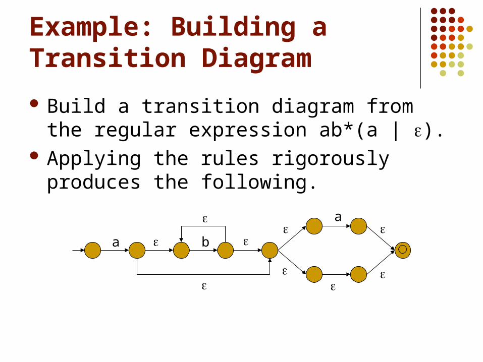
Build a transition diagram from the regular expression ab*(a | ).

Applying the rules rigorously produces the following.

a

b

a

Converting an NFA to a DFA

Let Q be the states of the NFA. The -closure of a state q in the NFA is the

set of all states that are reachable from q through sequences of -moves.

Define the states of the DFA to be (Q), i.e., sets of states in the NFA.

Converting an NFA to a DFA

For every state A (Q) and every symbol x , the transition (A, x) is the -closure of all states in the NFA that are reached from states in A by reading x.

Example: A DFA from an NFA

Consider the NFA of the regular expression ab*(a | ).

Number the states 1 through 10.

1 2 3 4 5

6 7

10

8 9

a

b

a


Find the -closure of each state. -cl(1) = {1}. -cl(2) = {2, 3, 5, 6, 8, 9, 10}. -cl(3) = {3}. -cl(4) = {3, 4, 5, 6, 8, 9, 10}. -cl(5) = {5, 6, 8, 9, 10}. -cl(6) = {6}. -cl(7) = {7, 10}.


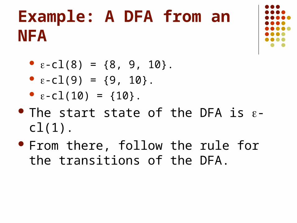
-cl(8) = {8, 9, 10}. -cl(9) = {9, 10}. -cl(10) = {10}.

The start state of the DFA is -cl(1). From there, follow the rule for the transitions

of the DFA.


The result is

a

b

a

ab 3, 4, 5, 6, 8, 9, 10

2, 3, 5, 6, 8, 9, 10 7, 101

Minimizing a DFA

To minimize a DFA is to reduce the number of states to a minimum without changing the language accepted by the DFA.

Two states p and q are equivalent if for every string w *, (p, w) and (q, w) are either both accepting states or both rejecting states.

Example: Minimizing a DFA

Minimize the DFA of regular expression ab*(a | ).

First, add a dead state to make the DFA fully defined.

1

5

2 3

4

a a

a a | ba | b b

bb


The initial partition is {1, 5}, {2, 3, 4}. Apply the transitions by a and b:

1 5 2 3 4

a 2 5 3 5 3

b 5 5 4 5 4

a distinguishes 1 and 5 and {2, 4} and 5.b distinguishes {2, 4} and 5.


The second partition is {1}, {2, 4}, {3}, {5}. a and b do not distinguish 2 and 4. Therefore, this is the final partition. States 2 and 4 are equivalent and should be

merged. Also, remove the dead state.


The minimized DFA is

1 2 3a a

b

Programming a DFA

There are two basic methods of programming a DFA. Use switch statements. Use a transition table.

Using Switch Statements

The main function contains a switch statement whose cases are the different states, including the dead state.

Each case contains a switch statement whose cases are the different symbols.

Example: DFASwitch.cpp

Using a Transition Table

The program uses a 2-dimensional array to store the transitions.

Rows represent states. Columns represent symbols. Example: DFATable.cpp

Symbol Tables

Identifiers are stored in a symbol table for future reference.

The symbol table contains essential information for each identifier. name type block level memory requirements scope.

Symbol Tables

When the lexer returns an identifier, the program looks it up in the symbol table.

If it is not there, it is added to the table.

Identifier Names

The value of the identifier, i.e., the name as a character string, is stored in a separate table of strings.

The symbol table entry contains a reference to the name in the string table.

Block Levels

There are three block levels in our compiler. Block level 1 – Keywords. Block level 2 – Global variables, including function

names. Block level 3 – Local variables, including function

parameters.

Keywords

A lexer becomes unnecessarily complicated if it must recognize each keyword in a language.

A simpler technique is to include the keywords in the symbol table.

The symbol table is initialized with the values of all keywords.

They are distinguished from other identifiers by having block level 0.

Syntax Analysis

Syntax Analysis

The syntax of a language is described by a context-free grammar.

Each grammar rule has the form

A where A is a nonterminal and is a string of terminals and nonterminals, i.e., ( N)*.

Grammar Convention

Terminals are represented by lowercase letters near the beginning of the alphabet (a, b, c, …) or by non-alphabetic characters (2, +, {, …).

Nonterminals are represented by uppercase letters near the beginning of the alphabet (A, B, C, …).

Grammar Convention

Grammar symbols that may be either terminals or nonterminals are represented by uppercase letters near the end of the alphabet (Z, Y, X, …).

Strings of terminals are represented by lowercase letters near the end of the alphabet (z, y, x, …).

Strings of grammar symbols (both terminals and nonterminals) are represented by lowercase Greek letters (, , , …).

Parsers

A parser is a program that Incorporates a grammar, Receives as input tokens from a lexer, and Outputs an abstract syntax tree representing the

grammatical structure of the input.

Parsing Algorithms

Parsing algorithms can be divided into two main categories.

Top-down parsers – Parse the input from top to bottom of a leftmost derivation.

Bottom-up parsers – Parse the input from bottom to top of a rightmost derivation.

Top-Down Parsers

There are two basic top-down methods of implementing a parser. Recursive descent parser. Table-driven parser (LL parsers).

Recursive Descent Parser

Each nonterminal in the grammar is implemented as a function.

Begin with the start symbol S of the grammar by calling function S().

Based on the first token received, apply the appropriate grammar rule for S.

Continue in this manner until S is “satisfied.”

Example: Recursive Descent

Write a parser for the following grammar.

S if C then S ; | while C do S ;

| id = num | id++

C id == num | id != num S represents a statement and C represents a

condition. Example: IfWhileParser.cpp

Example: Recursive Descent

Modify the previous example by adding the production

S' S S' | S' represents a sequence of statements. Modify the previous example by adding the

productions

S do S while C ;

C id < num

Recursive Descent Parsers

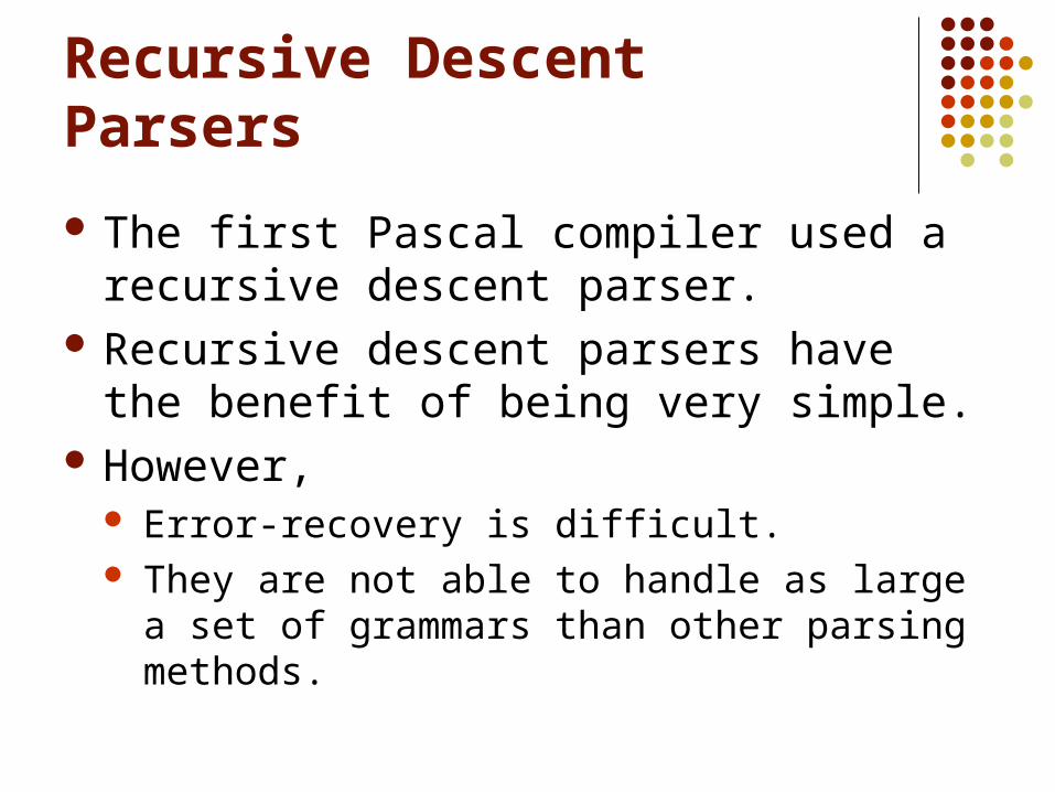
The first Pascal compiler used a recursive descent parser.

Recursive descent parsers have the benefit of being very simple.

However, Error-recovery is difficult. They are not able to handle as large a set of

grammars than other parsing methods.

Another Problem with Recursive Descent Parsers

Suppose the grammar were

S S S | a How could the parser decide how many times

to use the production S S S before using the production S a?

Futile Attempt #1

void S(){ if (token == a) match(a); else { S(); S(); }}

Futile Attempt #2

void S(){ if (token != EOF) { S(); S(); }}

Left Recursion

The method of recursive descent does not work if the grammar is left recursive.

A grammar is left recursive if there is a derivation

A + Afor some nonterminal A and string .

In particular, a production is left recursive if it is of the form

A A.

Left Recursion

Applying the method of recursive descent would lead to the function

void A(){ A();// Process }

which leads to infinite recursion.

Left Recursion

Recall that in the earlier example, we added the production

S' S S' | ,not the production

S' S' S | Why? Are they equivalent as far as the language of

the grammar is concerned?

Eliminating Left Recursion

Left recursion in a production may be removed by transforming the grammar in the following way.

Replace

A A | with

A A'

A' A' | .

Eliminating Left Recursion

Under the original productions, a derivation of is

A A A A . Under the new productions, a derivation of

is

A A' A' A'

A' .

Example: Eliminating Left Recursion

Consider the left recursive grammar

E E + T | T

T T * F | F

F (E) | id Apply the transformation to E:

E T E'

E' + T E' | .


Then apply the transformation to T:

T F T'

T' * F T' | .


Now the grammar is

E T E'

E' + T E' | .T F T'

T' * F T' | .F (E) | id


The function for E' would be

void Eprime(){ if (token == PLUS) { match(PLUS); T(); Eprime(); } return;}

Advantages of Left Recursion

A left recursive grammar is often more intuitive than the transformed grammar.

A left recursive grammar will match expressions earlier, leading to shallow recursion. Consider parsing a + b + c + d + e.

Bottom-up parsing takes advantage of the benefits of left recursion.

Left Factoring

A minor problem occurs when two productions for the same nonterminal begin with the same token.

We cannot decide which production to use.

This is not necessarily a problem since we could process they part they have in common, then make a decision based on what follows.

Left Factoring

Consider the grammar

A | . We use left factorization to transform it into

the form

A A'

A' | . Now we can apply the productions

immediately and unambiguously.

Example: Left Factoring

In the earlier example, we had the productions

C id == num | id != num | id < num To perform left factoring, introduce a

nonterminal C':

C id C'

C' == num | != num | < num

Example: Left Factoring

Consider the grammar of if statements.

S if C then S else S

| if C then S We rewrite it as

S if C then S S'

S' else S | .

LL Parsing

LL Parsing

LL parsing reads the tokens from Left to right and parses them top-down according to a Leftmost derivation.

Table-Driven Parsing

To build the parsing table, we need two functions FIRST FOLLOW

and the notion of nullability.

Nullability

A nonterminal A is nullable if

A * . Clearly, A is nullable if it has a production

A . But A is also nullable if there are, for example,

productions

A BC.

B A | aC | .C aB | Cb | .

Nullability

In other words, A is nullable if there is a production

A ,or there is a production

A B1B2…Bk,

where B1, B2, ..., Bk are nullable.

Nullability

In the grammar

E T E'

E' + T E' | .T F T'

T' * F T' | .F (E) | id

E' and T' are nullable. E, T, and F are not nullable.

FIRST and FOLLOW

Given a grammar G, we may define the functions FIRST and FOLLOW on the strings of symbols of G. FIRST() is the set of all terminals that may

appear as the first symbol in a replacement string of .

FOLLOW() is the set of all terminals that may follow in a derivation.

FIRST

For a grammar symbol X, FIRST(X) is defined as follows. For every terminal X, FIRST(X) = {X}. For every nonterminal X, if X Y1…Yn is a

production, then FIRST(Y1) FIRST(X).

Furthermore, if Y1, …, Yk are nullable, then

FIRST(Yk + 1) FIRST(X).

FIRST

We are concerned about FIRST(X) only for the nonterminals A of the grammar.

FIRST(X) for terminals a is trivial. According to the definition, to determine

FIRST(A), we must inspect all productions that have A on the left.

Example: FIRST

Let the grammar be

E T E'

E' + T E' | .T F T'

T' * F T' | .F (E) | id | num

Example: FIRST

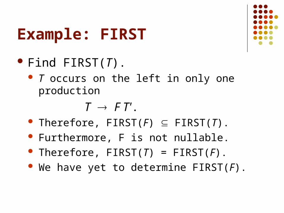
Find FIRST(E). E occurs on the left in only one production

E T E'. Therefore, FIRST(T) FIRST(E). Furthermore, T is not nullable. Therefore, FIRST(E) = FIRST(T). We have yet to determine FIRST(T).

Example: FIRST

Find FIRST(T). T occurs on the left in only one production

T F T'. Therefore, FIRST(F) FIRST(T). Furthermore, F is not nullable. Therefore, FIRST(T) = FIRST(F). We have yet to determine FIRST(F).

Example: FIRST

Find FIRST(F). FIRST(F) = {(, id, num}.

Therefore, FIRST(E) = {(, id, num}. FIRST(T) = {(, id, num}.

Example: FIRST

Find FIRST(E'). FIRST(E') = {+}.

Find FIRST(T'). FIRST(T') = {*}.

FOLLOW

For a grammar symbol X, FOLLOW(X) is defined as follows. If S is the start symbol, then $ FOLLOW(S). If A B is a production, then FIRST()

FOLLOW(B). If A B is a production, or A B is a

production and is nullable, then FOLLOW(A) FOLLOW(B).

FOLLOW

We are concerned about FOLLOW(X) only for the nonterminals A of the grammar.

According to the definition, to determine FOLLOW(A), we must inspect all productions that have A on the right.

Example: FOLLOW

Let the grammar be

E T E'

E' + T E' | .T F T'

T' * F T' | .F (E) | id | num

Example: FOLLOW

Find FOLLOW(E). E is the start symbol, therefore $ FOLLOW(E). E occurs on the right in only one production.

F (E). Therefore FOLLOW(E) = {$, )}.

Example: FOLLOW

Find FOLLOW(E'). E' occurs on the right in two productions.

E T E'

E' + T E'. Therefore, FOLLOW(E') = FOLLOW(E) = {$, )}.

Example: FOLLOW

Find FOLLOW(T). T occurs on the right in two productions.

E T E'

E' + T E'. Therefore, FOLLOW(T) contains FIRST(E') = {+}. However, E' is nullable, therefore it also contains

FOLLOW(E') = {$, )}. Therefore, FOLLOW(T) = {+, $, )}.

Example: FOLLOW

Find FOLLOW(T'). T' occurs on the right in two productions.

T F T'

T' * F T'. Therefore, FOLLOW(T') = FOLLOW(T) = {$, ), +}.

Example: FOLLOW

Find FOLLOW(F). T occurs on the right in two productions.

T F T'

T' * F T'. Therefore, FOLLOW(F) contains FIRST(T') = {*}. However, T' is nullable, therefore it also contains

FOLLOW(T') = {$, ), +}. Therefore, FOLLOW(F) = {*, $, ), +}.

Summary

Nonterminal Nullable FIRST FOLLOW

E No {(, id, num} {$, )}

E' Yes {+} {+, $, )}

T No {(, id, num} {$, ), +}

T' Yes {*} {$, ), +}

F No {(, id, num} {*, $, ), +}

Predictive Parsing Table

The parsing table has one row for each nonterminal, one column for each terminal and $.

Each entry in the table corresponds to a combination (A, a) of a nonterminal and a terminal.

Parsing Table Entries

Each table entry is a production A . Rules for A .

For every a FIRST(), write A in the (A, a) cell. If FIRST(), write A in the (A, a) cell for

every a, including $, in FOLLOW(). Write “error” in all other cells.

Parsing Table Entries

The interpretation of A in cell (A, ) is that if we are processing a string for A and we encounter , then we should “reduce” to A by applying the production.

Example: Parsing Table

Let the grammar be

E T E'

E' + T E' | .T F T'

T' * F T' | .F (E) | id | num


Consider E T E'. FIRST(T E') = FIRST(T) = {(, num, id}. Enter E T E' in cells (E, ( ), (E, num), (E, id).

Consider E' . is in FIRST() and FOLLOW(E') = {$, )}. Enter E' in cells (E', $) and (E', ) ).


The parsing table is

+ * ( ) num id $

E E TE' E TE' E TE'

E' E+TE' E' E'

T T FT' T FT' T FT'

T' T' T'*FT' T' T'

F F (E) Fnum F id

Predictive Parsing

A grammar is called LL(1) if its predictive parsing table does not contain any multiple entries.

A multiple entry would indicate that we couldn’t decide which production to apply.

Predictive Parsing Algorithm

The predictive parsing algorithm uses The parsing table, An input buffer containing a sequence of

tokens, A stack of grammar symbols.

Initially The input buffer contains the input followed by

a $. The stack contains $ on the bottom and S, the

start symbol, on the top.


Consider the top stack symbol X. There are three possibilities.

X is a terminal. X is a nonterminal. X is $.


If X is a terminal, then It must match the current token. If so, pop it and advance to the next token. If not, then that is an error.


If X is a nonterminal, then Use it and the current token to get the entry from

the parsing table. It should be a production. If not, then that is an error. Pop X from the stack. Push the symbols on the right-hand side of the

production, from right to left.


If X is $, then The current token should also be $. If not, then that is an error.

Example: Predictive Parsing

Parse the string (id + num)*id.$ E ( id + num ) * id $

$ E’ T ( id + num ) * id $

$ E’ T’ F ( id + num ) * id $

$ E’ T’ ) E ( ( id + num ) * id $

$ E’ T’ ) E id + num ) * id $

$ E’ T’ ) E’ T id + num ) * id $

$ E’ T’ ) E’ T’ F id + num ) * id $

$ E’ T’ ) E’ T’ id id + num ) * id $

$ E’ T’ ) E’ T’ + num ) * id $

$ E’ T’ ) E’ + num ) * id $


$ E’ T’ ) E’ T + + num ) * id $

$ E’ T’ ) E’ T + num ) * id $

$ E’ T’ ) E’ T num ) * id $

$ E’ T’ ) E’ T’ F num ) * id $

$ E’ T’ ) E’ T’ num ) * id $

$ E’ T’ ) E’ T’ ) * id $

$ E’ T’ ) E’ ) * id $

$ E’ T’ ) ) * id $

$ E’ T’ * id $

$ E’ T’ F * * id $


$ E’ T’ F id $

$ E’ T’ id id $

$ E’ T’ $

$ E’ $

$ $

Bottom-Up Parsing

Let the grammar be

E E + T | T

T T * F | F

F (E) | id | num

Rightmost Derivations

A rightmost derivation of (id + num)*id isE T

T*F T*id F*id (E)*id (E + T)*id (E + F)*id (E + num)*id (T + num)*id (F + num)*id (id + num)*id.

LR Parsers

A bottom-up parser follows a rightmost derivation from the bottom up.

Such parsers typically use the LR algorithm and are called LR parsers. L = process tokens from Left to right. R = follow a Rightmost derivation.

LR Parsers

An LR parser uses a parsing table, an input buffer, and a stack of “states.”

If performs three operations. Shift a token from the input buffer. Reduce the content of the stack by applying a

production. Change state.

LR(0) Items

To build an LR parsing table, we must first find the LR(0) items.

An LR(0) item is a production with a special marker () marking a position on the right side.

Example: LR(0) Items

If the production is

E E + T,

then the possible LR(0) items are [E E + T] [E E + T] [E E + T] [E E + T ]

LR(0) Items

The interpretation of [A ] is “We have processed and we might process next.”

Whether we actually do process will be borne out by the subsequent sequence of tokens.

LR Parsing

We build a PDA whose states are sets of LR(0) items.

First we augment the grammar with a new start symbol S'.

S' S. This guarantees that the start symbol will not

recurse.

States of the PDA

The initial state is called I0.

State I0 is the closure of the set

{[S' S]}. To form the closure of a set of items

For each item [A B] in the set and for each production B , add the item [B ] to the set.

Continue until there is no further change.

Example: LR Parsing

Continuing with the example, the augmented grammar is

E' E

E E + T | T

T T * F | F

F (E) | id | num

Example: LR Parsing

The state I0 consists of the items[E' E]

[E E + T][E T][T T * F][T F][F (E)][F id][F num]

Transitions

For each grammar symbol that immediately follows the marker , there will be a transition to another state.

If an item is [A X], then The transition occurs on processing symbol X, The transition is to the closure of the item [A X

].

Example: LR Parsing

From the state I0, there will be transitions for the symbols E, T, F, (, id, and num.

On processing E, the items

[E' E] and [E E + T]

become

[E' E ] and [E E + T].

Example: LR Parsing

Let state I1 be the closure of these items.

I1: [E' E ]

[E E + T] Thus the PDA has the transition

I0 I1

E

Example: LR Parsing

Similarly we determine the other transitions from I0.

Process T:

I2: [E T ]

[T T * F] Process F:

I3: [T F ]

Example: LR Parsing

Process (:I4: [F ( E)]

[E E + T][E T][T T + F][T F][F (E)][F id][F num]

Example: LR Parsing

Process id:

I5: [F num ] Process num:

I6: [F id ]

Example: LR Parsing

Now find the transitions from states I1 through I6 to other states, and so on, until no new states appear.

Example: LR Parsing

I7: [E E + T]

[T T * F]

[T F]

[F (E)]

[F id]

[F num]

Example: LR Parsing

I8: [T T * F]

[F (E)]

[F id]

[F num] I9: [F (E )]

[E E + T]

Example: LR Parsing

I10: [E T ]

[T T * F] I11: [E E + T ]

[T T * F] I12: [T T * F ] I13: [F (E) ]

The LR(0) Parsing Tables

There are two tables (which we will combine into one table).

The action table Contains shift and reduce actions upon

processing terminals. The goto table

Contains changes of state upon matching productions.

The Action Table

The action table contains one row for each state in the PDA and one column for each nonterminal and EOF ($).

The entries are Shift n – Push the current token and move to

state n. Reduce n – Pop symbols of right side of

production n and push the nonterminal of the left side. Then change state according to the goto table.

Building the Action Table

If [A a] is in state Ii and the PDA transition is

Ii Ij

a

then set the (i, a) entry to “shift j.”

Building the Action Table

If [A ] is in state Ii and A S', then set the (i, a) entry is “reduce A ” for all a in FOLLOW(A), including $.

If [S' S ] is in state Ii, then the (i, $) entry is “accept.”

The Goto Table

The goto table has one row for each state in the PDA and one column for each nonterminal except S'.

The entries are states of the PDA.

Building the Goto Table

If [A B] is in state Ii and the PDA transition is

then set the (i, B) entry to “goto j.”

Ii Ij

B

Example: LR Parsing

LRParsingTable.xls

Example: LR Parsing

Parse (id + num)*id.0 ( id + num ) * id $

0 ( 4 id + num ) * id $

0 ( 4 id 6 + num ) * id $

0 ( 4 F 3 + num ) * id $

0 ( 4 T 2 + num ) * id $

0 ( 4 E 9 + num ) * id $

0 ( 4 E 9 + 7 num ) * id $

0 ( 4 E 9 + 7 num 5 ) * id $

0 ( 4 E 9 + 7 F 3 ) * id $

0 ( 4 E 9 + 7 T 11 ) * id $

0 ( 4 E 9 ) * id $

Example: LR Parsing

0 ( 4 E 9 ) 13 * id $

0 F 3 * id $

0 T 2 * id $

0 T 2 * 8 id $

0 T 2 * 8 id 6 $

0 T 2 * 8 F 12 $

0 T 2 $

0 E 1 $

Accept $

CUP

Lecture x

X, Feb x, 2004

The Symbol Table

The Symbol Table

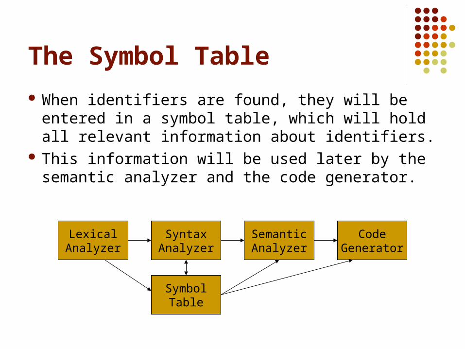
When identifiers are found, they will be entered in a symbol table, which will hold all relevant information about identifiers.

This information will be used later by the semantic analyzer and the code generator.

LexicalAnalyzer

SemanticAnalyzer

CodeGenerator

SymbolTable

SyntaxAnalyzer

Symbol Table Entries

We will store the following information about identifiers.

The name (as a string). The data type. The block level. Whether it has been defined. The number of bytes required. It’s scope (global, local, parameter). It’s offset from the base pointer (for local variables

only).

Symbol Table Entries

This information will not be known all at once. Typically, we begin by knowing only the

name and block level. Later we learn the data type, number of

bytes, scope, and the offset.

Symbol Table Functions

The two most basic symbol-table functions are the ones that insert a new symbol and lookup an old symbol. IdEntry install(String s, int blkLev); IdEntry idLookup(String s, int blkLev);

Inserting a Symbol

The install() function will insert a new symbol into the symbol table.

Each symbol has a block level. Block level 1 = Keywords. Block level 2 = Global variables. Block level 3 = Parameters and local variables.

install() will create an IdEntry object and store it in the table.

Inserting a Symbol

When the symbol is first encountered by the lexer, we do not yet know the scope or type.

That is determined later by the parser. For example, we could encounter the symbol count in any of the following contexts. int count; int func(int sum, float count); int main() {int count…}

Looking up a Symbol

Whenever a symbol is encountered, we must look it up in the symbol.

If it is the first encounter, then the lookup() function will return null.

If it is not the first encounter, then the lookup() function will return a reference to the IdEntry for that identifier found in the table.

Block Levels

Keywords, global variables, and local variables are stored at different block levels.

C and C++ recognize further levels (blocks) within functions, delimited by braces { }.

However, in C, variables local to a block must be declared at the beginning of the block.

Every time we enter a block, the block level increases by 1 and every time we leave a block, it decreases by 1.

Structure of the Symbol Table

We will implement the symbol table as a linked list of hashtables, one hashtable for each block level.

Level 3 Level 1Level 2

Hashtableof

Locals

Hashtableof

Globals

Hashtableof

Keywords


Initially, we install the keywords in the symbol table at level 1.

Level 1

Hashtableof

Keywords


Then we increase the block level and install the globals at level 2.

A new hashtable is inserted at the head of the list.

Level 1Level 2

Hashtableof

Globals

Hashtableof

Keywords


When we enter a function, we insert a new, level 3 hashtable at the head of the list.

Local variables are installed at this level.


Hashtableof

Locals

Hashtableof

Globals

Hashtableof

Keywords


When we leave the function, the hashtable of local variables is deleted from the list.

Level 1Level 2

Hashtableof

Globals

Hashtableof

Keywords

Locating a Symbol

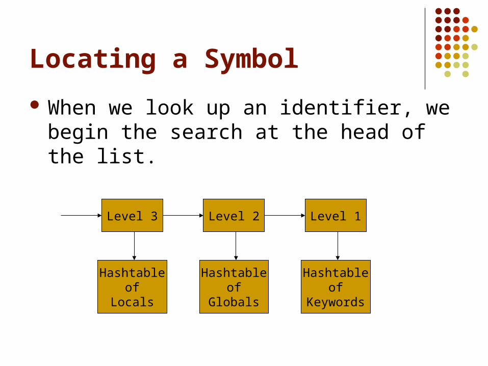
When we look up an identifier, we begin the search at the head of the list.


Hashtableof

Locals

Hashtableof

Globals

Hashtableof

Keywords

Locating a Symbol


The search continues at the lower levels.


Hashtableof

Locals

Hashtableof

Globals

Hashtableof

Keywords

Looking up a Symbol


The search continues at the lower levels.


Hashtableof

Locals

Hashtableof

Globals

Hashtableof

Keywords

Looking up a Symbol

If an identifier is declared both globally and locally, which one will be found when it is looked up?

How do we prevent the use of a keyword as a variable name?

Distinguishing Between Keywords and Identifiers

The keywords are installed at level 1 before the lexer begins.

When the lexer finds an “identifier,” it looks it up in the symbol table.

If it finds it at level 1, it returns the appropriate keyword token.

Otherwise, it returns an identifier token.

Distinguishing Between Keywords and Identifiers

The benefit of this is that it greatly simplifies the lexer.

For example, imagine that a program has identifiers el, els, and elses.

The regular expression for true identifiers would be awful.

However, in JLex, we would solve that problem by listing the keywords’ regular expressions first, then the regular expression for identifiers.

Hashtables

A hashtable is a list in which each member is accessed through a key.

The key is a value that is derived from the value to be looked up in the table.

The function that produces a key from a value is called the hash function.

For example, if it were a hashtable of strings, the key might be the sum of the ASCII values of the first 5 characters of the string, modulo the size of the table.

Hashtables

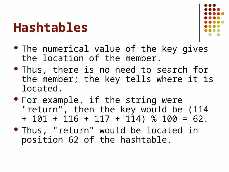
The numerical value of the key gives the location of the member.

Thus, there is no need to search for the member; the key tells where it is located.

For example, if the string were "return", then the key would be (114 + 101 + 116 + 117 + 114) % 100 = 62.

Thus, "return" would be located in position 62 of the hashtable.

Hashtables

Clearly, there is the possibility of a clash: two members happen to have the same key.

In that case, the hashtable creates a short list of those values in the table with that same key.

When that key comes up, the list is searched. However, it is generally a very short list,

especially if the table size has been chosen well.

Hashtables in Java

Java has a Hashtable class. Look it up on the web to see what it’s

member functions are. The Java Hashtable class will use it’s own

hash function to create the keys. The two most important functions (for us) are

put() and get().

String Tables

Compilers generally create a table of strings. These strings are the “names” of the

identifiers. Thus, if the same string is used for several

different identifiers, they string will be stored only once in the string table.

Each symbol table entry will include a pointer to the string in the string table.

For simplicity, we will not use a string table.

Abstract Syntax Trees


The abstract syntax tree (AST) shows the logical structure of the program or part of the program.

The parse tree shows every token that is returned by the lexer.

The AST shows only those tokens that are necessary for the semantics of the program.

Indeed, the AST may have nodes that correspond to no token.


Recursive descent parsers generally create a single AST for the entire program.

Our parser will generate a separate AST for each statement. It will create a list of ASTs. This will allow us to generate assembly code as

the ASTs are created. The trees will be connected sequentially and

through jump statements.

Syntax-Directed Definitions

A syntax-directed definition is a context-free grammar with attributes added to the grammar symbols.

Each symbol has A set of synthesized attributes, and A set of inherited attributes.

Synthesized Attributes

A synthesized attribute of a grammar symbol is a property that is determined by the properties of symbols below it in the AST.

In other words, if A is a production, then A’s synthesized attributes are determined by the attributes of the symbols in .

Example: Synthesized Attributes

If the AST represents a numerical expression, then the value of the root node is determined by the values of the nodes below it in the tree.


Let the grammar be

E E + E | num Then E derives its value from the num tokens

in the expression. This is expressed formally by the rules

E.val = E1.val + E2.val,

E.val = num.lexval.


E.val

E1.val

num.lexvalnum.lexval

E2.val+

Synthesized Attributes

The terminals would get their values directly from the lexical analyzer.

For example, a NUM token’s value attribute would be the numerical value of the string of digits in the token.

Inherited Attributes

An inherited attribute is an attribute of a symbol (node) that is determined by its parent node and its siblings.

In other words, if is symbol on the right side of the production A , then ’s inherited attributes are determined by the attributes of A and the other symbols in .

Example: Inherited Attributes

Consider the grammar for a declaration containing one or more identifiers.

D T L

L L , id | id

T int | float For example, the declaration might be

int a, b;


D

T.type

id1.typefloat

L.type

id2.type

ba


The attribute (float) first appears as the value of the t token.

From there it is passed to the identifier a. Then it is passed to the identifier b.

Question

In an expression tree, is the type of the expression inherited or is it synthesized?

Example: Expression Tree

We will describe how to build an AST for an expression.

We will use TreeNode constructors TreeNode(op, left, right) TreeNode(id, entry) TreeNode(num, value)


To construct a tree for the expression

a - 4 + c

we do the following: ptr1 = new TreeNode(id, entry_a)

ptr2 = new TreeNode(num, 4)

ptr3 = new TreeNode(minus, ptr1, ptr2)

ptr4 = new TreeNode(id, entry_c)

ptr5 = new TreeNode(plus, ptr3, ptr4)


The semantic rules would be

Production Semantic Rule

E E1 + T E.ptr = new TreeNode(plus, E1.ptr, T.ptr);

E E1 – T E.ptr = new TreeNode(minus, E1.ptr, T.ptr);

E T E.ptr = T.ptr;

T (E) T.ptr = E.ptr;

T id T.ptr = new TreeNode(id, id.entry);

T num T.ptr = new TreeNode(num, num.val);

x86 Architecture

Lecture 15

Mon, Mar 15, 2004

Overview

See the reference“IA-32 Intel® Architecture Software Developer's Manual Volume 1: Basic Architecture”

at

ftp://download.intel.com/design/Pentium4/manuals/25366513.pdf

Instructions

Each instruction is of the formlabel: opcode operand1, operand2, operand3

The label is optional. The number of operands is 1, 2, or 3,

depending on the opcode. Each operand is either

An immediate value, or A register, or A memory address.

Instructions

Each operand is either a source operand or an destination operand.

A source operand, in general, may be An immediate value, A register, or A memory address.

A destination operand, in general, may be A register, or A memory address.

Instructions

Some instructions are more restrictive. Not every logical combination is permitted in

every instruction.

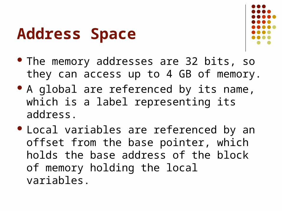
Address Space

The memory addresses are 32 bits, so they can access up to 4 GB of memory.

A global are referenced by its name, which is a label representing its address.

Local variables are referenced by an offset from the base pointer, which holds the base address of the block of memory holding the local variables.

Basic Registers

There are Eight 32-bit general-purpose registers, One 32-bit EFLAGS register, One 32-bit instruction pointer register (EIP), and Other special-purpose registers.

The General-Purpose Registers

The eight 32-bit general-purpose registers are eax, ebx, ecx, edx, esi, edi, ebp, and esp.

For calculations, we will use eax, ebx, ecx, and edx. esp is the stack pointer. ebp is the base pointer. esi and edi are source and destination index

registers for array and string operations. Even though they are general purpose, we should

avoid using ebp, esi, edi, and esp for other purposes.

The General-Purpose Registers

The registers eax, ebx, ecx, and edx may also be accessed as 16-bit or 8-bit registers.

For example, The two low-order bytes of eax may be accessed

through the name ax. The high-order byte of ax is named ah. The low-order byte of ax is named al.

The other three registers are similarly structured and named.

The General-Purpose 32-Bit Registers

eaxebxecxedxebpesiediesp

accumulator

base pointer

stack pointer

string source

string destination


bpsidisp

dxcxbxax


ah albh blch cldh dl

EFLAGS Register

The various bits of the 32-bit EFLAGS register are set (1) or reset (0) according to the results of certain operations.

We will be interested only in the bits CF – carry flag PF – parity flag ZF – zero flag SF – sign flag

Instruction Pointer

Finally, there is the eip register, which is the instruction pointer.

eip holds the address of the next instruction to be executed.

We should never use eip or change its value.

Data Types

There are 5 integer data types. Byte – 8 bits. Word – 16 bits. Doubleword – 32 bits. Quadword – 64 bits. Double quadword – 128 bits.

We will use doublewords unless we have a specific need for one of the others.

The Run-time Stack

The run-time stack supports procedure calls and the passing of parameters between procedures.

The stack is located in memory. The stack grows in a downward direction. In other words, decrementing esp will grow

the stack, while incrementing esp will shrink the stack.

Using the Run-time Stack

Typically, when we perform an operation, we will push the result onto the stack.

The next operation, if it expects a previous result, will pop it off the stack.

The alternative is to use the registers to pass results, but that is more complicated since we would have to keep track of which registers were free.

Function Calls and the Base Pointer

When we make a function call, we use the base pointer ebp to store the top of the stack before the function call.

esp ebp Then we push the parameters and local

variables of the function onto the stack. When we return from the function, we use the

base pointer to restore the stack to its previous state.

ebp esp

The Instruction Set

Lecture 16

Wed, Mar 17, 2004

The Runtime Stack

The runtime stack is a portion of memory that used as a stack during program execution.

The address of the top of the stack is stored in the register esp, called the stack pointer.

The stack grows in a “downward” direction. When values are pushed, esp is decremented. When values are popped, esp is incremented.

The Runtime Stack

esp points to the “top” of the stack.

Stack

esp

The Runtime Stack

Push a value and decrement esp.

Stack

esp

The Runtime Stack

Push another value and decrement esp again.

Stack

esp

The Runtime Stack

Pop a value and increment esp.

Stack

esp

The Runtime Stack

Pop another value and increment esp again.

Stack

esp

The Push and Pop Instructions

The push and pop instructions have the format

push source

pop destination The source is a register, a memory address,

or an immediate value. The destination is a register or a memory

address.

The Push and Pop Instructions

The push instruction will increment the stack pointer and then move source to the stack.

The pop instruction will move the value on the stack to destination and then decrement the stack pointer.

Processing the Syntax Tree

The syntax tree is processed in a post-order traversal.

At each node Process the left subtree. Process the right subtree. Process the node.

Using the Stack

As each node of the syntax tree is executed, it will leave its result on the run-time stack.

The next node will pop that result off the stack (if it needs it) and then push its own result onto the stack, and so on.

Example

The syntax tree for a = b + c – 5 is

ASSIGN

MINUSNAME

a

PLUS

DEREF

NUM5

DEREF

NAMEb

NAMEc

Example

Execution NAME – Push the address of a. NAME – Push the address of b. DEREF – Push the value of b. NAME – Push the address of c. DEREF – Push the value of c. PLUS – Pop the values, add them, push the result. NUM – Push 5. MINUS – Pop the values, subtract them, push the result. ASSIGN – Pop the value and the address, store the value

at the address, push the result.

A NUM Node

A NUM node loads the integer whose value is stored in the node.

For example, to load 5:push $5

The $ sign means the “immediate” value 5.

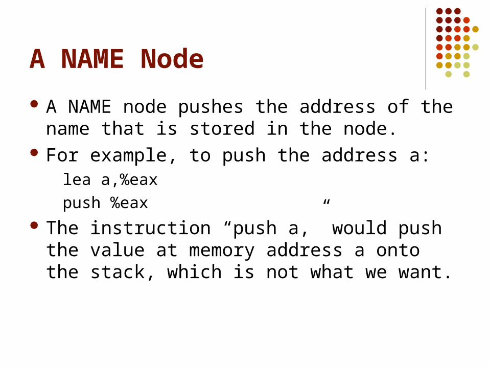
A NAME Node

A NAME node pushes the address of the name that is stored in the node.

For example, to push the address a:lea a,%eax

push %eax The instruction “push a,” would push the

value at memory address a onto the stack, which is not what we want.

A DEREF Node

A DEREF node expects to find a memory address on top of the stack.

It pushes the value stored at that address.pop %eax

push (%eax) The parentheses mean “the value at the

address in the register.” This is the indirect addressing mode.

The Add Instruction

The add instruction has the formatadd source,destination

The value at source is added to the value at destination and the result is stored at destination.

source is a register, a memory address, or an immediate value.

destination is a register or a memory address.

A PLUS Node

A PLUS node expects to find two numbers on the stack.

The right operand should be on top. It pops the values, adds them, and pushes

the result.pop %edxpop %eaxadd %edx,%eaxpush %eax

An ASSIGN Node

An ASSIGN node expects to find an address and a value on the stack.

The value should be on top. It pops the value and the address, stores the

value at the address, and pushes the value.pop %eax

pop %edx

mov %eax,(%edx)

push %eax

The imul Instruction

The imul instruction performs multiplication of signed integers.

The first format

imul source source is one operand. eax is the other operand. The destination is edx:eax, which holds a 64-bit

value.


The second formatimul register,source

source is one operand. It is a register, a memory address, or an immediate

value. register is the other operand and the destination.


The third formatimul register,source,immediate

register is the destination. source is one operand.

It is a register, a memory address, or an immediate value.

immediate is the other operand.

A TIMES Node

A TIMES node expects to find two values on the stack.

It pops them, multiplies them, and pushes the result.pop %eax

pop %ecx

imul %ecx

push %eax

The x87 FPU

Lecture n

Date

The x87 Registers

compiler design coms 480 spring 2004. the syllabus the syllabus

Documents