comparison of sequential indicator simulation, object
TRANSCRIPT

Accepted Manuscript
Comparison of sequential indicator simulation, object modelling and multiple-pointstatistics in reproducing channel geometries and continuity in 2D with two differentspaced conditional data sets
Fengde Zhou, Daren Shields, Stephen Tyson, Joan Esterle
PII: S0920-4105(18)30229-8
DOI: 10.1016/j.petrol.2018.03.043
Reference: PETROL 4784
To appear in: Journal of Petroleum Science and Engineering
Received Date: 2 February 2016
Revised Date: 29 January 2018
Accepted Date: 8 March 2018
Please cite this article as: Zhou, F., Shields, D., Tyson, S., Esterle, J., Comparison of sequentialindicator simulation, object modelling and multiple-point statistics in reproducing channel geometriesand continuity in 2D with two different spaced conditional data sets, Journal of Petroleum Science andEngineering (2018), doi: 10.1016/j.petrol.2018.03.043.
This is a PDF file of an unedited manuscript that has been accepted for publication. As a service toour customers we are providing this early version of the manuscript. The manuscript will undergocopyediting, typesetting, and review of the resulting proof before it is published in its final form. Pleasenote that during the production process errors may be discovered which could affect the content, and alllegal disclaimers that apply to the journal pertain.

MANUSCRIP
T
ACCEPTED
ACCEPTED MANUSCRIPT
1
Comparison of Sequential Indicator Simulation, Object
Modelling and Multiple-point Statistics in Reproducing Channel
Geometries and Continuity in 2D with Two Different Spaced
Conditional Data Sets
Fengde Zhou a,b, Daren Shields a, Stephen Tyson a,b,c, Joan Esterle a,b
a School of Earth and Environmental Sciences, University of Queensland, Brisbane, Qld
4072, Australia
b Centre for Coal Seam Gas, University of Queensland, Brisbane, Qld 4072, Australia
c Universiti Teknologi Brunei, BE1410 Brunei Darussalam
ABSTRACT
Fluvial sediments with multi-scale channels are difficult to model using classical two-point
statistical methods, e.g. sequential indicator simulation (SIS) or object-based modelling
(ObjM). Multiple-point statistics (MPS) has been used to generate facies, fracture and
porosity distributions based on pattern statistics derived from training datasets. However, the
ability of these three methods to reproduce channel geometry and continuity is not clear,
especially when using differently spaced conditional data. This paper presents a case study to
compare the application of these three methods in reproducing channels from a section of
Amazon River based on two differently spaced conditional data sets. Results show that: the
reproduction accuracy is similar between MPS and SIS; MPS provides the most connected
channel facies (or most channel continuity) as compared to SIS and ObjM; and using a hand-

MANUSCRIP
T
ACCEPTED
ACCEPTED MANUSCRIPT
2
drawn facies based on the sampling points yield a similar accuracy to that achieved by using
the reality facies distribution as the training image. Finally, we conclude that the application
of MPS does not significantly increase the reproduction accuracy when compared to SIS
channel models; however, MPS can generate realistic models with respect to channel
geometry and continuity.
Keywords: Sequential indicator simulation; Object modelling; Multiple-point statistics;
Channel geometry and continuity; Amazon River.
1. INTRODUCTION
Fluvial channels may be broadly classified on the basis of channel sinuosity and
multiplicity into four-part taxonomy including straight, braided, meandering and
anastomosing river systems (Rust, 1977; Miall, 2014). Individually, these channels can
include up to 17 types of discrete lithologies grouped into 8 architectural elements (Miall,
2006). Due to the inherent complexity of these systems resulting in severe heterogeneity,
channel systems have been the focus for many researchers (Chen et al., 2015).
In geological modelling, sequential indicator simulation (SIS) and object modelling
(ObjM) are widely used to populate categorical variables such as facies, while multiple-point
statistics (MPS) is used comparatively less due to its inherent complexity and practical
limitations such as increased run time and practical issues such as (1) uncertainty in
geological scenarios, (2) scanning template (or search mask) and non-stationarity (Strebelle
and Zhang, 2004; Eskandari and Srinivasan, 2010), and (3) subjectively in training image
selection (Strebelle, 2002). Stationarity, one of the main requisites for the construction of a
valid training image, requires the mean and variance of a variable be constant throughout a
model area. In reality, this is seldom the case for most geological systems at regional scales.

MANUSCRIP
T
ACCEPTED
ACCEPTED MANUSCRIPT
3
SIS populates properties using variogram models, which describe the change of linear
correlation with increasing offset – a technique known as two-point geostatistics (Journel,
1983; Journel and Isaaks, 1984; Journel and Alabert, 1988; Deutsch, 2006). This method is
most appropriate if (1) the shape of particular facies bodies is not clear (Pyrcz and Deutsch,
2014), or (2) with a high density of conditional data, e.g. with close well spacing or dense 3D
seismic data (Zhou et al., 2016). Facies distributions generated by SIS can appear patchy or
unstructured when unconstrained by secondary data (Deutsch, 2006). ObjM, also known as
marked point process (Haldorsen and Chang, 1986; Haldorsen and MacDonald, 1987;
Haldorsen and Damsleth, 1990; Holden et al., 1998) or Boolean simulation (Seifert and
Jensen, 2000), populates facies based on pre-defined geometries (i.e., objects) rather than
two-point geostatistics. Facies fraction, orientation, amplitude, wavelength, width, and
thickness are some of the input parameters needed to define the objects for ObjM (Holden et
al., 1998; Manzocchi et al., 2007; Stephen et al., 2001). MPS, a pixel-based sequential
simulation algorithm, is capable of producing models with more geological complexity than
SIS and better honours hard data than ObjM (Strebelle and Journel, 2001; Strebelle, 2002;
Mariethoz et al., 2010; Rezaee et al., 2015). In particular, MPS generates models by
rendering complex facies connectivity patterns which may be critical for the prediction of
fluid flow and transport problems (Mariethoz et al., 2010). Applications of the algorithm
have ranged from a simulation of a fluvial reservoir facies using different training images and
nested sequences (Strebelle, 2002) to modelling porosity distributions in a carbonate reservoir
(Zhang et al., 2006). MPS has also been used to generate facies and fracture distributions
(Erzeybek et al., 2012; Peredo and Ortiz, 2012; Stuart et al., 2014). In practice, ObjM uses
multiple iterations to place the geo-bodies into the 3D grid, and hence requires longer run-
times to honour hard data as compared to either SIS or MPS (Caers, 2001; Strebelle and
Journel, 2001; Strebelle, 2002; Caers and Zhang, 2004; Liu et al., 2004). Additionally, ObjM

MANUSCRIP
T
ACCEPTED
ACCEPTED MANUSCRIPT
4
may not honour all hard data, e.g. facies fraction or object geometries particularly with
respect to datasets with an abundance of hard data.
To understand the difference between SIS, ObjM and MPS, Bastante et al. (2008)
compared these three methods in modelling slate deposits. They concluded that the estimated
useful slate percentages by MPS were much closer to reality than indicator Kriging (IK) or
SIS but the results relied partly on information obtained via IK. Larriestra and Gomez (2010)
compared SIS, ObjM and MPS for a high sinuosity fluvial system and concluded that channel
probability modes were represented more realistically by MPS than other modelling
techniques. De Iaco and Maggio (2011) compared the predicted spatial distribution of
limestone by SIS and MPS and concluded that MPS better reproduced the spatial distribution
of limestone and meandering channels. Though these three modelling methods have been
tested, evaluated and compared in the oil and gas industry, comparing the effectiveness of
SIS, ObjM and MPS in reproducing channel distribution with different spaced data has not
been adequately covered in academia. While data spacing plays a critical role in geological
modelling.
2. DATA AND METHODOLOGY
2.1. Data
This study focuses on one section of the Amazon River (Fig. 1a), located in Brazil near
the Atlantic Ocean. An area of 80×80 km2 was digitised and imported into PetrelTM (Fig. 1b).
Figures show that there are three distinct orders (scales) of channels which can be classified
based on their unique depositional architectures, e.g. into primary, secondary and tertiary
channels with widths of approximately 8 km, 3 km and 1 km, respectively. The areal
fractions are 17.8%, 8.1% and 6.4% for primary, secondary and tertiary channels,
respectively (Fig. 1b). The total areal fractions are 32.3% and 67.7% for channel and
MANUSCRIP
T
ACCEPTED
ACCEPTED MANUSCRIPT
5
floodplain respectively. In the following study, we combined primary, secondary and tertiary
channels as one facies of channel in modelling because we have no training image for each of
these channels.
Fig. 2 shows the sampled data points (used as model inputs) using two different spacings,
e.g. 2.5 km and 5.0 km. Fig. 2a shows data points with sampling spacing of 2.5 km. We can
see most points consist of primary channels and partial secondary channels, hence primary
and secondary channels will be well represented in the model. If a sampling interval of 5.0
km is used, most sample points are from primary channels hence only the primary channel
will be adequately represented in the models. The original fraction calculated from these data
points was used as the target input statistic in the modelling process.
2.2. Methodology
The intent of this paper is to compare the ability of SIS, ObjM and MPS to reproduce
channel geometry and continuity by assessing the reproduction accuracy and facies
connectivity of models constructed with the various methods. Note that the accuracy in
geomodelling is better measured by assessing the geological models by means of dynamic
simulation, in which the behaviour of a static grid is interrogated by varying dynamic
conditions. In this study, the reproduction accuracy means the ratio of cells, which have same
facies as the given facies distribution, to the total cells in the model. The conditional data
(hard data) were sampled based on the digitised facies distribution with two different
spacings of 5.0 km and 2.5 km respectively.
The algorithms for SIS, ObjM and MPS are briefly described herein; however, for a
more comprehensive background regarding the application of these three techniques readers
are referred to Bastante et al. (2008). Table 1 presents the comparison of steps for these three
methods.

MANUSCRIP
T
ACCEPTED
ACCEPTED MANUSCRIPT
6
The indicator approach used by SIS transforms facies into binary variables when dealing
with categorical variables like facies (Falivene et al., 2006). SIS is based on indicator kriging
which gives an estimation of relative proportions of the different facies. SIS generates a
random sequential path for property population using a pseudo-random number generator that
allows the user to enter a given seed values so that multiple stochastic runs are repeatable.
Each other unknown location within a grid is sequentially visited and a value for the variable
is estimated based on the predicted relative probabilities.
In ObjM, object facies were introduced to replace a background facies such as
undifferentiated floodplain sediments or marine shales (Falivene et al., 2006). The geometric
and dimensional ranges of the introduced object facies are defined to reproduce the
variability of sedimentary elements in the depositional model (Haldorsen and Chang, 1986;
Clementsen et al., 1990; Tyler et al., 1994; Deutsch and Wang, 1996; Deutsch and Tran,
2002). The algorithm begins by finding a point in the model which has the same facies code
as the body; then makes a body for the given facies with its predefined geometry; then the
body is located in the model to honour hard data. These processes iterated until the object
facies proportions, which are generally considered as the most critical parameter (Falivene et
al., 2006), are consistent with facies global fraction.
MPS is based on a stationary training image which can be generated using densely and
regularly sampled field-data (Okabe and Blunt, 2005), photographs of outcrops or aerial
photographs processed with a computer-aided design (CAD) algorithm, ObjM (Bastante et al.,
2008) or hand-drawn models (Zhou et al., 2016). A training image is a 3D model defining the
typical geometries and relationships that will be converted to conditional probability
distributions known as a multi-point facies pattern. The training image is used to define the
neighbourhood relationship of respective facies by creating patterns defined by probability
distribution functions (pdf). During the pattern creation, multi-grids (Strebelle, 2002) are used

MANUSCRIP
T
ACCEPTED
ACCEPTED MANUSCRIPT
7
to describe both small and large-scale structures, similar to short and long variogram ranges if
using two-point geostatistics (Okabe and Blunt, 2005; Xu et al., 2012). The multi-grids
concept was initially proposed by Gómez-Hernández (1991) and Tran (1994). The multi-
grids number and search radius are provided in an ellipsoid search mask to create the patterns.
Using different multi-grid schemes yields different results (Comunian et al., 2012; Straubhaar
and Malinverni, 2014). In MPS modelling, the digitised distribution of channels and
floodplain in Fig. 1 is used as the training image. The MPS algorithm of SNESIM, introduced
by Strebelle (2002), in PetrelTM was used in MPS modelling.
Fig. 3a is a training image with a channel areal ratio of 26%. This area is gridded into
400 cells. According to the events’ template with four neighbour conditioning data (Fig. 3b),
the data event number is 24=16 (Fig. 3b); then we can account for the probability of each
event globally as shown in Table 2. For example, there are 168 grids are cross-connected
with four neighbouring grids at event #1 (EV1); 5 of those 168 grids are channel facies.
3. RESULTS AND DISCUSSION
3.1. Modelling results with data sampling space of 2.5 km
Based on a sampling space of 2.5 km, the input fraction of channels is 32.5% which is
similar to the actual volume channel percentage of 32.3%. In order to use SIS, we first
analyse the horizontal indicator variogram using a maximum search distance in x- and y-
direction of 60 km and a lag distance of 10 km. Fig. 4a shows the generated horizontal
variogram map which indicates a major orientation of about 45˚. We then generated the
directional variogram along major and minor orientation respectively. The lag distance is 2
km and the number of lags is 30 for both major and minor orientation. The band-width is 2.5
km; tolerance angle is 45˚; lag tolerance is 50%. Fig. 4b and 4c show the experimental
standardised semivariance (Zhou et al., 2015) and its regressions. Results show that the sill is

MANUSCRIP
T
ACCEPTED
ACCEPTED MANUSCRIPT
8
1.08 and major and minor ranges are 16.2 km and 7.4 km respectively. The major and minor
ranges from indicators are similar to the maximum width and length of the channel facies
(Guo and Deutsch, 2010).
SIS is used to generate the facies distributions as shown in Fig. 5 with nine realisations
based on the results of variogram analysis. Results show that the primary channel polygons
are filled with channels, reflecting the techniques generally high accuracy of reproducing
primary channels; however, the secondary and tertiary channels are more difficult to
reproduce because their major and minor orientations are not the same as the inputs. If the
secondary and tertiary channels are given different facies codes, they can have different
variograms with different orientations. Also, if the variogram model has nested structures the
short-range structures can have different orientation and anisotropy to the longer structures.
This study combined all the channels and the accuracies are quantified in section 3.3.
In ObjM input fractions and geometries, e.g. orientation, amplitude, wavelength, width,
thickness, and trends for channels are defined a priori. Table 3 lists the modelling parameters
used in which the channel orientation is taken from the variogram analysis while channel
width is derived from the digitised statistics. The amplitude and wavelength are assumed as
listed in Table 3 because they are difficult to be measured for the channels in Fig. 1. In ObjM,
we selected honouring hard data as the honouring priority and Fig. 6 shows that ObjM
struggles to honour all hard data. In addition, it is a time-consuming technique with
approximately 3hrs required to generate 9 realisations compared to several minutes for
equivalent SIS or MPS models. It is worth noting that changing the inputs, e.g. channel
geometry, trends may improve the conditioning of hard data and modelling accuracy.
In MPS modelling, the digitised distribution of channels and floodplain in Fig. 1 is used
as the training image. Ellipsoid search mask with a radius of 10 grid nodes and number of
multi-grids of 3 is used to create the patterns. Note that the ellipsoid search mask defined in
MANUSCRIP
T
ACCEPTED
ACCEPTED MANUSCRIPT
9
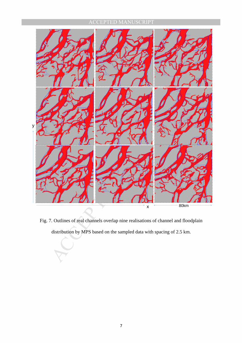
PetrelTM, which uses the SNESIM code, is quantified in nodes. In this study, the simulation
grid size is same as the training image so no scaling is needed. Fig. 7 shows nine realisations
which indicate a good match for the primary channel and significant characterisation of
secondary and tertiary channels.
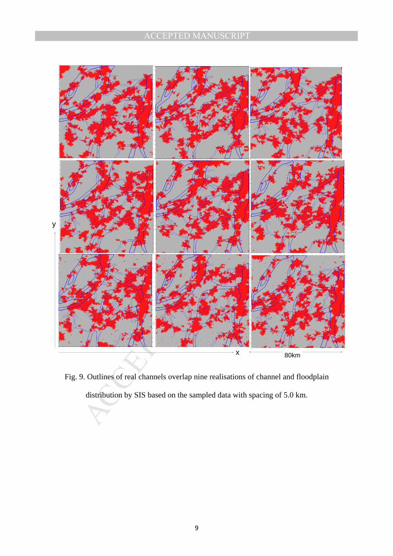
3.2. Modelling results with data sampling spacing of 5.0 km
With a sampling space of 5.0 km, the fraction of channels (the ratio of sampling points
met with channel facies to the total number of sampling points) is 36.0%, which is higher
than the actual value of 32.3% calculated from the digitised map. This result indicates that
there is often a bias for the calculated fraction of channels from sampling points even with a
regular data sampling spacing. In order to compare the results with the actual distributions as
shown in Fig. 1b, a channel fraction of 32.3% was used to generate subsequent models. Fig.
8a shows that the horizontal variogram indicates a major range orientation of about 80˚. The
major and minor ranges are 14.5 km and 11.8 km respectively (Figs. 8b and 8c), which
indicate that the heterogeneity describing capacity decreases with the increase of sampling
spacing. Note that the histogram of pairs suggests an inadequate sampling (non-homogenous)
and the experimental variogram is distorted.
Fig. 9 shows the nine realisations of channel and floodplain distribution by SIS based on
the sampled data with a spacing of 5.0 km. Results indicate that the estimated channel at right
side matches well with the digitised image. The accuracy is higher than 90% for the largest
channel in the right-hand image.
Fig. 10 shows the nine realisations of channel and floodplain distribution by MPS based
on the sampled data with a spacing of 5.0 km. Results indicate that the estimated channels
match well with the digitised image at some locations.

MANUSCRIP
T
ACCEPTED
ACCEPTED MANUSCRIPT
10
3.3. Accuracy comparison in reproducing channels
The accuracy, which is defined as the ratio of the matched grid number between
estimations and the digitised image over the total number of grids, is used to compare the
modelling results from different methods each with nine realisations. Based on the sampled
data points with spacing of 2.5 km, the accuracy of SIS results ranges from 81% to 82% with
an average of 81%; for MPS results, it ranges from 83% to 85% with an average of 84%; for
ObjM results, it ranges from 57% to 65% with an average of 62%. Based on sampled data
points with spacing of 5.0 km, the accuracy for SIS results ranges from 67% to 71% with an
average of 70%; for MPS results, it ranges from 68% to 74% with an average of 71%. Note
that the variogram for the floodplain is same as for the channels for a two facies model. The
modelling results using the channel as the background facies are similar with those using
floodplain as the background facies.
3.4. Comparison of channel connectivity
Journel et al. (1989) used a multiple step connectivity experiments to assess the
geological modelling results. In this study, geometrical modelling is used to generate the
distribution of connected volumes (bodies; Fig. 11). The probability of each connected
volume is calculated based on the summation of juxtaposed grid blocks containing the
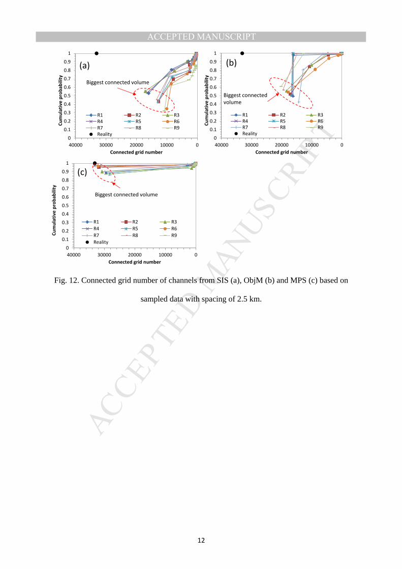
channel facies code. Fig. 12 shows the cumulative probability for connected channels
generated from SIS, ObjM and MPS based on sampled data with a spacing of 2.5 km. Results
show that MPS has the greatest proportion of connected channels. Results show that the
probability of the biggest connected channels ranges from 32% to 55% with an average of 45%
by SIS; ranges of 43% to 61% with an average of 52% by ObjM; and ranges from 87% to 97%
with an average of 92% by MPS. The probability of connected channels is 100% in Fig. 1b
which indicates MPS results match well with reality. Note that assuming a complete set of

MANUSCRIP
T
ACCEPTED
ACCEPTED MANUSCRIPT
11
connected channel sands is hardly ever the case in a subsurface sedimentary record.
Integration and representation of thin shale layers, their lateral extension and potential impact
on flow behaviour are the challenges in the modelling of lobes and channel architecture
(Falivene et al., 2006). Bastante et al. (2008) also reported that areas of slate by MPS are
more regular and continuous than other methods.
Fig. 13 shows the cumulative probability of connected channels from SIS, ObjM and
MPS based on sampled data with a spacing of 5.0 km. Results show that the probability of
the biggest connected channels ranges from 30% to 78% with an average of 45% by SIS and
ranges from 79% to 99% with an average of 89% by MPS. This indicates that the uncertainty
increases with increasing data sampling spacing. Results by MPS match well with reality
based on sampled data with a spacing of 5.0 km.
As reported by Caers and Zhang (2004), subsurface reservoir modelling is undertaken to
produce models that accurately predict global flow properties while also estimating local
recoverable grades of ore in mining. Therefore, the channel connectivity is an important
factor on fluid flow and recoverable volumes. The connectivity in this study is quite simple
which does not address more geological details, such as the relationships of connectivity with
net: gross ratio and dynamic performance (Larue and Hovadik, 2006; Pranter, 2014).
3.5. Training image
Generating training images using densely and regularly sampled data (Okabe and Blunt,
2005), photographs of outcrops or aerial photographs processed with a computer-aided design
(CAD) algorithm, ObjM and hand-drawn models may contradict the non-stationary
requirement for training images. Image patterns, sourced from a training image, record the
probability of each event (Zhou et al., 2016) regardless of the location of these events in the
training image; hence MPS models cannot preserve the non-stationary features of the training

MANUSCRIP
T
ACCEPTED
ACCEPTED MANUSCRIPT
12
image (Strebelle and Zhang, 2004). Nested methods using several auxiliary variables, e.g.
zones, distances, facies belt and rotation angles, as trend information were used to model
non-stationary reservoir characteristics (Strebelle and Zhang, 2004; Yin et al., 2015), but the
process requires known trends of the object property for locating the non-stationary reservoir
characteristics.
Generating a training image by combining hard data and soft data from the whole object
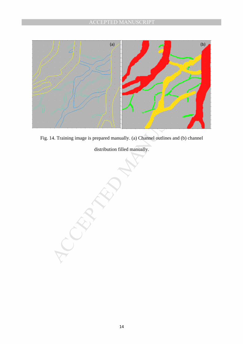
field will reduce the effect of non-stationary problems (Lorentzen et al., 2012). Figs. 14a and
13b show the processes to prepare a training image manually based on the sampled hard data
with a spacing of 5.0 km and current direction and channel size. Note that the width of the
secondary channel and the tertiary channel is assumed as 2.5 km and 1.0 km, respectively.
Three steps are used in mapping channels; firstly, outline the primary channel according to
the channel direction; then outline secondary channel which has similar flow trend as primary
channel but also distribute between channels; the tertiary channel is outlined according to its
width and flow direction of the primary and secondary channel. Facies are mapped based on
the outline as shown in Fig. 14b then are converted into binary (categorical) facies, channel
(including primary, secondary and tertiary channels) and floodplain. The distributed binary
facies are used as training images for creating the MPS patterns.
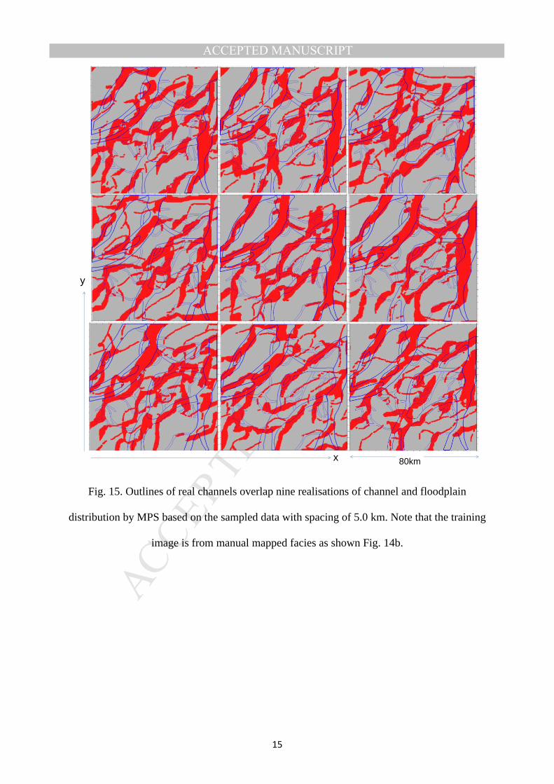
Fig. 15 shows the simulated facies distribution with nine realisations. The accuracy of
estimation of channels compared with reality ranges from 64% to 73% with an average of
69%. Results show that the accuracy is similar to that achieved by using the reality facies
distribution as the training image.

MANUSCRIP
T
ACCEPTED
ACCEPTED MANUSCRIPT
13
4. CONCLUSIONS
In this study, a section of Amazon River is used to compare the application of SIS, ObjM
and MPS in reproducing channels based on the digitised facies distribution in 2D with two
different sampling spacing, 2.5 km and 5.0 km.
The reproducing accuracy by MPS is similar to that by SIS but higher than that by ObjM
which was run with drilling data and channel orientation. Dense conditional data leads to
high accuracy in reproducing facies distribution which means the harder data available to
condition the simulations, the more deterministic the simulations become. MPS generated
better-connected model than ObjM and SIS. Results by MPS match better with reality for the
biggest connected channels than those produced by SIS and ObjM. However, generating a
robust training image for MPS is still challenging in geological modelling. ObjM was used in
generating the training images because it can well capture the shape and geometry of
depositional bodies. This study shows that a manually generated training image yields a
similar accuracy to that achieved by using real facies distribution as the training image.
ACKNOWLEDGEMENT
We acknowledge the Centre for Coal Seam Gas and its member companies (APLNG,
Arrow Energy, QGC and Santos) for the support and Schlumberger for providing the license
of PetrelTM. We thank Helen Schultz for comments and corrections. We also thank the
anonymous reviewers for providing the constructive comments.
REFERENCES
Bastante, F.G., Ordonez, C., Taboada, J., Matias, J.M., 2008. Comparison of indicator kriging,
conditional indicator simulation and multiple-point statistics used to model slate deposits.
Engineering Geology 98, 50-59.

MANUSCRIP
T
ACCEPTED
ACCEPTED MANUSCRIPT
14
Caers, J., Zhang, T., 2004. Multiple-point geostatistics: a quantitative vehicle for integrating
geologic analogs into multiple reservoir models. In: Grammer, G. M., Harris, P. M.,
Eberli, G. P (Eds.). Integration of outcrop and modern analogs in reservoir modeling.
AAPG Memoir 80, 383-394.
Chen, S., Lin, C., Liu, W., 2015. 3D geological modelling method of fluvial facies
considering the information of sedimentary process. EJGE 20(6), 1487-1497.
Comunian, A., Renard, P., Straubhaar, J., 2012. 3D multiple-point statistics simulation using
2D training images. Computers & Geosciences 40, 49-65.
De Iaco, S., Maggio, S., 2011. Validation Techniques for Geological Patterns Simulations
Based on Variogram and Multiple-Point Statistics. Mathematical geosciences 43, 483-
500.
Deutsch, C.V., 2006. A sequential indicator simulation program for categorical variables with
point and block data: BlockSIS. Computers & Geosciences 32, 1669-1681.
Deutsch, C.V., Journel, A.G., 1998. GSLIB Geostatistical Software Library and User's Guide.
Second Edition.
Erzeybek, S., Srinivasan, S., Janson, X., 2012. Multiple-point statistics in a Non-gridded
domain: Application to karst/fracture network modeling. Quantitative Geology and
Geostatistics 17, 221-237.
Eskandari, K., Srinivasan, S., 2010. Reservoir Modelling of Complex Geological Systems--A
Multiple-Point Perspective. Journal of Canadian Petroleum Technology 49, 59-68.
Falivene, O., Arbués, P., Gardiner, A., Pickup, G., Muñoz, J.A., Cabrera, L., 2006. Best
practice stochastic facies modelling from a channel-fill turbidite sandstone analog (the
Quarry outcrop, Eocene Ainsa basin, northeast Spain. AAPG Bulletin 90(7), 1003-1029.

MANUSCRIP
T
ACCEPTED
ACCEPTED MANUSCRIPT
15
Gómez-Hernández, J., 1991. A stochastic approach to the simulation of block fields’
conductivity upon data measured at a smaller scale. PhD thesis, Stanford University,
Stanford.
Guo, H., Deutsch, C.V., 2010. Fluvial channel size determination with indicator variograms.
Petroleum Geoscience 16, 161-169.
Haldorsen, H.H., Chang, D.M., 1986. Notes on stochastic shales from outcrop to simulation
models. In Reservoir Characterization, ed. Lake, L.W. and Carol, H.B., pp. 152-167.
New York, USA: Academic.
Haldorsen, H.H., Damsleth, E., 1990. Stochastic modelling. Journal of Petroleum Technology
42(4), 404-412.Holden, L., Hauge, R., Skare, O., Skorstad, A., 1998. Modeling of fluvial
reservoirs with object models. Mathematical Geology 30, 473-496.
Haldorsen, H.H., MacDonald, C.J., 1987. Stochastic modelling of underground reservoir
facies (SMURF). SPE paper 16751 presented at the 62nd Annual Technical Conference
and Exhibition held in Dallas, Texas.
Journel, A.G., 1983. Nonparametric estimation of spatial distribution. Mathematical Geology
15 (3), 445-468.
Journel, A.G., Alabert, F.G., 1988. Focusing on spatial connectivity of extreme valued
attributes: stochastic indicator models of reservoir heterogeneities, SPE Paper 18324.
Journel, A.G., Isaaks, E.H., 1984. Conditional indicator simulation: application to a
Saskatchewan uranium deposit. Mathematical Geology 16 (7), 685-718.
Journel, A.G., Journal, A.G., Alabert, F., 1989. Non-Gaussian data expansion in the Earth
Sciences. Terra nova (Oxford, England) 1, 123-134.
Larue, D.K., Hovadik, J., 2006. Connectivity of channelized reservoirs: a modelling approach.
Petroleum Geoscience 12, 291-308.

MANUSCRIP
T
ACCEPTED
ACCEPTED MANUSCRIPT
16
Larriestra, C.N., Gomez, H., 2010. Multiple-point simulation applied to uncertainty analysis
of reservoirs related to high sinuosity fluvial systems: Mina EI Carmen Formation, San
Jorge Gulf Basin, Argentina. AAPG International Conference and Exhibition, Rio de
Janeiro, Brazil, November 15-18, 2009.
Liu, Y., Rusty Gilbert, A.H., Journel, A., 2004. A workflow for multiple-point geostatistical
simulation. In Geostatistics Banff, eds. Leuangthong, O., Deutsch, C.V., pp. 245-254.
Netherlands: Springer.
Lorentzen, R.J., Flornes, M., Naevdal, G., 2012. History matching channelized reservoirs
using the Ensemble Kalman Filter. SPE Journal 17(1), 137-151.
Manzocchi, T., Walsh, J.J., Tomasso, M., Strand, J., Childs, C., Haughton, P.D.W., 2007.
Static and dynamic connectivity in bed-scale models of faulted and unfaulted turbidites.
In: Jolley, S.J., Barr, D., Walsh, J.J., Knipe, R.J. (eds) Structurally Complex Reservoirs,
Geological Society, London, Special Publications, 292, 309-336.
Mariethoz, G., Renard, P., Straubhaar, J., 2010. The direct sampling method to perform
multiple-point geostatistical simulations. Water Resources Research 46, W11536,
doi:10.1029/2008WR007621.
Miall, A.D., 2014. Chapter 2: The facies and architecture of fluvial systems. In: Fluvial
depositional systems. Springer Geology. Springer International Publishing Switzerland.
Miall, A.D., 2006. Reconstructing the architecture and sequence stratigraphy of the preserved
fluvial record as a tool for reservoir development: a reality check. AAPG Bulletin 90(7),
989-1002.
Okabe, H., Blunt, M.J., 2005. Pore space reconstruction using multiple-point statistics.
Journal of Petroleum Science and Engineering 46, 121-137.

MANUSCRIP
T
ACCEPTED
ACCEPTED MANUSCRIPT
17
Peredo, O., Ortiz, J.M., 2012. Multiple-point geostatistical simulation based on genetic
algorithms implemented in a shared-memory supercomputer. Quantitative Geology and
Geostatistics 17, 103-114.
Pranter, M.J., 2014. Fluvial architecture and connectivity of the Williams Fork Formation,
Piceance Basin, Colorado: combining outcrop analogs and reservoir modelling for
stratigraphic reservoir characterization. Search and Discovery Article #50959,
presentation at Oklahoma City Geological Society, January, 2014, and Tulsa Geological
Society, February 25, 2014.
Pyrcz, M.J., Deutsch, C.V., 2014. Geostatistical Reservoir Modeling, Oxford University
Press, 2nd edition, USA, pp236.
Rezaee, H., Marcotte, D., Tahmasebi, P., Saucier, A., 2015. Multiple-point geostatistical
simulation using enriched pattern databases. Stochastic Environmental Research and
Risk Assessment 29, 893-913.
Rust, B.R, 1977. A Classification of Alluvial Channel Systems. Fluvial Sedimentology —
Memoir 5, 187-198.
Seifert, D., Jensen, J.L., 2000. Object and pixel-based reservoir modeling of a braided fluvial
reservoir. Mathematical Geology 32(5), 581-603.
Stephen, K.D., Clark, J.D., Gardiner, A.R., 2001. Outcrop-based stochastic modelling of
turbidite amalgamation and its effects on hydrocarbon recovery. Petroleum Geoscience 7,
163-172.
Straubhaar, J., Malinverni, D., 2014. Addressing Conditioning Data in Multiple-Point
Statistics Simulation Algorithms Based on a Multiple Grid Approach. Mathematical
geosciences 46, 187-204.
Strebelle, S.B., 2002. Conditional simulation of complex geological structures using
multiple-point statistics. Mathematical Geology 34, 1-21.

MANUSCRIP
T
ACCEPTED
ACCEPTED MANUSCRIPT
18
Strebelle, S.B., Journel, A.G., 2001. Reservoir modeling using multiple-point statistics. SPE
paper 71324 presented at the SPE Annual Technical Conference and Exhibition held in
New Orleans, Louisiana, 1–11.
Strebelle, S.B., Zhang, T., 2004. Non-stationary multiple-point geostatistical models. In:
Leuangthong, O., Deutsch, C.V. (Eds.), Geostatistics Banff, 2004, 235-244.
Stuart, J., Moundney, N.P., McCaffrey, W.D., Lang, S., Collinson, J.D., 2014. Prediction of
channel connective and fluvial style in the flood basin successions of the Upper Permian
Rangal Coal Measures (Queensland). AAPG Bulletin 98(2), 191-212.
Tran, T., 1994. Improving variogram reproduction on dense simulation grids. Computers &
Geosciences 20, 1161–1168.
Xu, Z., Teng, Q.Z., He, X.H., Yang, X.M., Li, Z.J., 2012. Multiple-point statistics method
based on array structure for 3D reconstruction of Fontainebleau sandstone. Journal of
Petroleum Science and Engineering 100, 71-80.
Yin, Y., Zhang, C., Li, S., 2015. A Location-Based Multiple Point Statistics Method:
Modeling the Reservoir With Non-Stationary Characteristics. AAPG Annual Convention
and Exhibition, Denver, CO., May 31 - June 3, 2015
Zhang, T., Bombarde, S., Strebelle, S.B., Oatney, E., 2006. 3D Porosity Modeling of a
Carbonate Reservoir Using Continuous Multiple-Point Statistics Simulation. SPE
Journal 11(3), 375-379.
Zhou, F., Shields, D., Tyson, S., Esterle, J., 2016. Nested approaches to modelling swamp
and fluvial channel distribution in the Upper Juandah Member of the Walloon Coal
Measures, Surat Basin. The AAPEA Journal 56, 81-100.
Zhou, F., Yao, G., Tyson, S., 2015. Impact of geological modelling processes on spatial
coalbed methane resource estimation. International Journal of Coal Geology 146, 14-27.

MANUSCRIP
T
ACCEPTED
ACCEPTED MANUSCRIPT
1
Table 1. Comparison of workflows between SIS, ObjM and MPS.
SIS (Deutsch and Journel, 1998)
ObjM (Petrel, 2014) MPS (Liu et al., 2004)
1. Establish grid system;
2. Assign data to the nearest grid node;
3. Build a random path through all of the grid nodes by seed number;
4. Search nearby data and previously simulated grid nodes;
5. Construct the conditional probabilities by Kriging;
6. Draw a value from conditional distribution;
7. Check results.
1. Find a point having the same facies code as the body;
2. Make a body with the given facies and geometry for the body;
3. Choose a random insertion point on the body;
4. Calculate the body thickness at the insertion point;
5. Search for that thickness among the upscalled wells still left to be honoured ;
6. Ensure that the body about to be inserted does not conflict with other upscalled cells;
7. If the body passes these checks, insert the body;
8. Loop from 2-7 until the global fraction is satisfied.
If no soft information is available, the steps are: 1. Scan training image to calculate the
conditional probability, P(A|B), for facies A at data events B. P(A|B) is stored in the form of a tree called a multi-point facies pattern;
2. Define a random path to visit each unknown node u
3. Generate a probability for visiting node;
4. At location u, read B(u) with hard data plus previously simulated values; then retrieve conditional probability; P(A|B)(u) according to B(u);
5. Draw a value (facies) according to P(A|B)(u) and step (3) generated probability;
6. Repeat steps (3) to (5) till visited all unknown node.

MANUSCRIP
T
ACCEPTED
ACCEPTED MANUSCRIPT
2
Table 2. Statistic of global event probability and grid channel probability (Zhou et al.,
2016).
Data event Grid numbers
Event probability, % Channel probability, % Channel Floodplain
EV1 5 163 42 3.0 EV2 5 9 3.5 35.7 EV3 7 16 5.75 30.4 EV4 10 4 3.5 71.4 EV5 3 19 13.6 9.1 EV6 0 0 0 0.0 EV7 6 0 1.5 100.0 EV8 30 37 16.75 44.8 EV9 26 43 17.25 37.7 EV10 1 0 0.25 100.0 EV11 1 2 0.75 33.3 EV12 5 0 1.25 100.0 EV13 2 1 0.75 66.7 EV14 3 1 1 75.0 EV15 0 0 0 0.0 EV16 1 0 0.25 100.0

MANUSCRIP
T
ACCEPTED
ACCEPTED MANUSCRIPT
3
Table 3. Parameters used in ObjM.
Parameters Distribution Min Mean Max Orientation Triangular 30˚ 45˚ 50 ˚ Amplitude Triangular 6km 8km 10km Wavelength Triangular 10km 15km 20km Width Triangular 1.5km 7.4km 10km
Thickness Not applicable because of 2D models were built
Trends Not used

MANUSCRIP
T
ACCEPTED
ACCEPTED MANUSCRIPT
1
Fig. 1. Earth view of one section of Amazon River near Atlantic Ocean (a) and digitized
channel and floodplain distribution (b). The location of study area is uploaded as an
Interactive Map Data (KMZ). Note that the width of tertiary channel is enlarged in
digitization and some small channels were ignored. The enlargement is help to visualize it in
modelling.
80km
80km
80
km
8km
3km
1km 80
km
(a) (b)
Primary channel
Tertiary channel
Secondary channel

MANUSCRIP
T
ACCEPTED
ACCEPTED MANUSCRIPT
2
Fig. 2. Sampled data with spacing of 2.5 km (a) and 5.0 km (b). Red points were sampled
from channel and grey points were sampled from floodplain.
(a) (b)

MANUSCRIP
T
ACCEPTED
ACCEPTED MANUSCRIPT
3
Fig. 3. A training image with marked event number (a) according to its 16 data events
with four conditioning data (b) (Zhou et al., 2016). Filled grids=channel; blank=floodplain.
1 1 1 1 9 4 5 1 1 1 1 3 9 4 5 1 1 1 1 1
1 1 1 3 9 14 5 1 1 1 1 9 12 8 5 1 1 1 1 1
1 1 1 9 12 8 5 1 1 1 9 9 8 8 1 1 1 1 1 4
1 1 3 9 8 8 1 1 1 9 9 8 8 1 1 1 1 1 9 1
1 1 9 7 8 1 1 1 9 9 8 8 1 1 1 1 1 3 4 8
1 1 9 8 5 1 1 9 9 14 8 1 1 1 1 1 1 9 7 5
1 9 7 8 1 1 9 9 13 14 11 1 1 1 1 1 3 9 8 5
3 9 8 5 1 9 9 8 13 12 11 11 1 1 1 1 9 2 8 1
9 2 8 1 9 9 8 8 3 12 16 5 5 1 1 9 4 8 1 1
1 8 1 9 9 8 8 1 3 12 8 8 1 1 3 9 8 5 1 1
2 1 9 9 8 8 1 1 9 2 8 1 1 1 9 2 8 1 1 4
1 9 9 8 8 1 1 9 4 8 1 1 1 9 1 8 1 1 9 4
9 9 8 8 1 1 9 9 8 5 1 1 9 4 14 1 1 3 9 8
3 8 8 1 1 9 3 8 8 1 1 3 9 13 5 5 1 9 7 8
2 2 1 1 3 4 8 2 1 1 4 9 2 8 2 1 9 9 8 5
1 1 1 1 9 7 5 1 1 9 9 5 8 1 1 9 3 8 8 1
1 1 1 3 9 8 5 1 9 3 8 8 1 1 9 4 8 2 1 1
1 1 4 9 7 8 1 9 1 8 2 1 1 9 9 8 5 1 1 1
1 9 9 10 8 5 9 4 8 1 1 1 9 3 8 8 1 1 1 1
3 3 8 8 2 3 3 8 5 1 1 3 1 8 2 1 1 1 1 1
(b)
(a)
uu1
u2u3
u4

MANUSCRIP
T
ACCEPTED
ACCEPTED MANUSCRIPT
4
Fig. 4. Horizontal variogram (a), variogram along major direction (45˚; b) and variogram
along minor direction (135˚; c). Note that the distance scale is 1:10 to reality.
(a)
(b)
(c)
45˚
135˚
Type: ExponentialSill: 1.08Major range: 16.2 km
Type: ExponentialSill: 1.04Minor range: 7.4 km
100 1100 2100 3100 4100 5100 61000
.25
0.5
0.7
51
Sem
ivar
ian
ce
0
Distance, m
100 1100 2100 3100 4100 5100 6100
0.2
50
.50
.75
1
Sem
ivar
ian
ce
0
Distance, m
1.2
5

MANUSCRIP
T
ACCEPTED
ACCEPTED MANUSCRIPT
5
Fig. 5. Outlines of real channels overlap nine realisations of channel and floodplain
distribution by SIS based on the sampled data with spacing of 2.5 km.
80km
y
x

MANUSCRIP
T
ACCEPTED
ACCEPTED MANUSCRIPT
6
Fig. 6. Outlines of real channels overlap nine realisations of channel and floodplain
distribution by ObjM based on the sampled data with spacing of 2.5 km.
80km
y
x
MANUSCRIP
T
ACCEPTED
ACCEPTED MANUSCRIPT
7
Fig. 7. Outlines of real channels overlap nine realisations of channel and floodplain
distribution by MPS based on the sampled data with spacing of 2.5 km.
80km
y
x

MANUSCRIP
T
ACCEPTED
ACCEPTED MANUSCRIPT
8
Fig. 8. Horizontal variogram (a), variogram along major direction (80˚; b) and variogram
along minor direction (170˚; c) based on the sampled data with spacing of 5.0 km (Fig. 2b).
Note that the map scale is 1:10 to reality.
(a)
(b)
(c)
80˚
170˚
Type: ExponentialSill: 1.04Major range: 14.5 km
Type: ExponentialSill: 1.04Minor range: 11.8 km
125 1875 3625 5375 7125 88750
.25
0.5
0.7
51
Sem
ivar
ian
ce
0Distance, m
125 1875 3625 5375 7125 8875
0.2
50
.50
.75
1
Sem
ivar
ian
ce
0
Distance, m
1.2
5
MANUSCRIP
T
ACCEPTED
ACCEPTED MANUSCRIPT
9
Fig. 9. Outlines of real channels overlap nine realisations of channel and floodplain
distribution by SIS based on the sampled data with spacing of 5.0 km.
80km
y
x

MANUSCRIP
T
ACCEPTED
ACCEPTED MANUSCRIPT
10
Fig. 10. Outlines of real channels overlap nine realisations of channel and floodplain
distribution by MPS based on the sampled data with spacing of 5.0 km.
80km
y
x

MANUSCRIP
T
ACCEPTED
ACCEPTED MANUSCRIPT
11
Fig. 11. Connected channels for realisation No.1 from SIS (a), ObjM (b) and MPS (c) based
on sampled data with spacing of 2.5 km. Different colour represents different connected body.
(a) (b) (c)
MANUSCRIP
T
ACCEPTED
ACCEPTED MANUSCRIPT
12
Fig. 12. Connected grid number of channels from SIS (a), ObjM (b) and MPS (c) based on
sampled data with spacing of 2.5 km.
0
0.1
0.2
0.3
0.4
0.5
0.6
0.7
0.8
0.9
1
010000200003000040000
Cu
mu
lati
ve p
rob
abili
ty
Connected grid number
R1 R2 R3R4 R5 R6R7 R8 R9Reality
Biggest connected volume
0
0.1
0.2
0.3
0.4
0.5
0.6
0.7
0.8
0.9
1
010000200003000040000
Cu
mu
lati
ve p
rob
abili
ty
Connected grid number
R1 R2 R3R4 R5 R6R7 R8 R9Reality
Biggest connected volume
0
0.1
0.2
0.3
0.4
0.5
0.6
0.7
0.8
0.9
1
010000200003000040000
Cu
mu
lati
ve p
rob
abili
ty
Connected grid number
R1 R2 R3
R4 R5 R6
R7 R8 R9
Reality
Biggest connected volume
(a) (b)
(c)

MANUSCRIP
T
ACCEPTED
ACCEPTED MANUSCRIPT
13
Fig. 13. Connected channels from SIS (a) and MPS (b) based on sampled data with spacing
of 5.0 km.
0
0.1
0.2
0.3
0.4
0.5
0.6
0.7
0.8
0.9
1
010000200003000040000
Cu
mu
lati
ve p
rob
abili
ty
Connected grid number
R1 R2 R3 R4
R5 R6 R7 R8
R9 Reality
Biggest connected volume
0
0.1
0.2
0.3
0.4
0.5
0.6
0.7
0.8
0.9
1
010000200003000040000
Cu
mu
lati
ve p
rob
abili
ty
Connected grid number
R1 R2 R3R4 R5 R6R7 R8 R9Reality
Biggest connected volume(a) (b)
MANUSCRIP
T
ACCEPTED
ACCEPTED MANUSCRIPT
14
Fig. 14. Training image is prepared manually. (a) Channel outlines and (b) channel
distribution filled manually.
(a) (b)
MANUSCRIP
T
ACCEPTED
ACCEPTED MANUSCRIPT
15
Fig. 15. Outlines of real channels overlap nine realisations of channel and floodplain
distribution by MPS based on the sampled data with spacing of 5.0 km. Note that the training
image is from manual mapped facies as shown Fig. 14b.
80km
y
x

MANUSCRIP
T
ACCEPTED
ACCEPTED MANUSCRIPT
1
Highlights
• Multiple-point statistics is used in reproducing an active river’s distribution.
• Sequential indicator simulation, object modelling and multiple-point statistics are
compared.
• Two different dense data sets are used in modelling and compared for results.