An Object Oriented Sequential Network Modelling Approach

Oscar Córdoba Muñoz - Inmaculada de Castro García

ITP, Madrid, Spainoscar.cordoba@itp.es

inmaculada.castro@itp.es

ABSTRACTThis document is the result of the experience acquired creating a tool for Gas Turbines Performance and FluidSystems modelling but most of the issues encountered are applicable to different networks problems (electricallines, pipe routing or control). The text compiles mathematical, numerical and methodological issues encounteredin the process.In this work an object oriented modelling approach is followed to simulate a network. Once a topology is created,the next step is to establish the most appropriate set of algebraic equations to characterise the problem. Thisprocess comprises the proper selection of equations, unknowns and sets of initial conditions that will allow thecorrect resolution of the system using a Newton Raphson algorithm, trying to avoid Jacobian matrix singularities.When this is not possible, instead of changing the solution method, other alternatives, as a multilevel strategy, areused.

NOMENCLATURE

A Geometric AreaCd Discharge coefficientc̄p Mean specific heat capacity at constant pressure∆T Temperature Difference ∆T = Toutlet −Tinlet

FP Flow parameterM Mach numberP Static pressurePt Total pressurePR Pressure Ratio PR = Pinlet

Poutlet

Q HeatTt Total temperatureTR Temperature Ratio T R = Toutlet

Tinlet

Re Reynolds numberSAS Secondary Air SystemW Mass flowγ Ratio of specific heat capacities

INTRODUCTIONThe main types of fluid systems found in a Gas Turbine are Oil, Fuel and Secondary Air Systems. These systems

are connected to the main gas path. The main gas path discipline is known as Gas Turbine Performance. Secondary AirSystems will be used as example to illustrate the main content of this work. A Gas Turbine Secondary Air System modelis usually understood as a model that represents the elements apart from the main gas path where the air passes usuallyfor sealing and cooling tasks. The different elements encountered in this sort of systems are pipes, orifices, nozzles,etc. and they are represented as components. The different components are linked representing the different ways ofthe flow, resulting in a network, with a defined topology. These models are commonly referred as 0D since there is nocontinuous characterisation through the fluid lines. Air system description is only available in stations before and afterthe components. The biggest challenges in the Air Systems, compared to Gas Turbine Performance models, are chokingand reverse flow phenomena. In the Gas Turbine Performance area, banks of initial guesses may be employed to converge

1

Proceedings of

11th European Conference on Turbomachinery Fluid dynamics & Thermodynamics

ETC11, March 23-27, 2015, Madrid, Spain

OPEN ACCESS

Downloaded from www.euroturbo.eu Copyright © by the Authors

towards the solution, Reference 4. This strategy cannot be used in Secondary Air Systems where even the flow directionis unknown.

Once a network topology is created, the next step is to establish the physical equations, mass conservation, momentumand energy conservation, for the individual components, coupling and boundary conditions. Everything in the documentis related to steady state although it is extensive to transient simulations. The mathematical model associated to this sortof physical problems in steady state is a system of nonlinear equations. The main targets are:

• To obtain which is the most appropriate set of equations and unknowns to be solved.

• To obtain which is the best set of initial conditions.

• To come up with the mathematical difficulties encountered applying the solving method.

The solution method for the algebraic nonlinear equations to be considered is Newton Raphson. If a set of equations issolved with Newton Raphson method, it will be considered robust enough. ~F (~x) = 0 is the system to solve. J = ∇~F

∣∣∣~xis

called Jacobian matrix at −→x . Three main causes for method failure will be listed:

• The value~xn obtained during the iterative process is out of an expected range. It may lead to negative temperaturesor pressures for instance.

• The inverse J−1 does not exist because the Jacobian matrix is singular. A local minimum or maximum is reached.A division by zero appears calculating the Jacobian matrix.

• The value J−1 does not exist because there is an infinite in the Jacobian matrix.

The three cases mentioned above may be overcome with an appropriate solver but other alternatives, as multilevel strategyor proper selection of tearing variables, will be discussed in the sequel.

Although there are commercial tools able to solve these problems, an in house development allows customisationsand the control of the physical methodology used. The selected approach enables unique models with components fromdifferent disciplines, such as Performance, Oil or Air Systems, as well as tailored features not existing in the market at thebeginning this work.

In the next sections the different alternatives to approach network models will be discussed. Based on the SecondaryAir Systems problem, some issues found using the selected approach will be presented. Finally, according to the exposedexamples, the main guidelines followed to address the resultant systems of nonlinear equations will be summarised.

EQUATION ORIENTED VERSUS SEQUENTIAL APPROACHESAn equation oriented approach creates an overall nonlinear algebraic system of equations to be computed globally.

This approach is widely discussed in Reference 3. On the other hand, a sequential solver computes each network com-ponent getting outputs for given inputs, solving nested equations if necessary. Each nested system of equations mustdecrease the solving tolerance; otherwise a deeply nested process may conflict with the computer rounding error. If thenested systems are not accurately solved, the outer system may observe that for the same unknown inputs could obtaindifferent residue values finding the solution.

The main idea is that there are better and worse approaches for specific problems rather than discussing the betterapproach. It is possible to find examples where one approach is better than the other. In Figure 1 the equation orientedapproach fails using the Newton Raphson method for the initial values that make singular the Jacobian of the system ofequations. In this example, the sequential approach never fails. In Figure 2 the equation oriented approach never fails andthere are initial values with singular Jacobian in the sequential approach. Each specific problem requires a study of thebest way to be performed.

The main advantages of an equation oriented approach are:

• Reduce problems with numerical tolerances. All the equations are solved at the same time with the same precision.

• The need of successive passes through the network and nested convergence at the unit operation level, make thesequential approach expensive in some cases.

On the other hand the advantages of sequential approaches are:

• Higher robustness may be implemented if inner iterations are properly done. There are some cases where someequations added to the overall system of equations may lead to convergence problems.

• Better debugging capabilities. The physical relations coded are not merged to be solved all together, as in theequation oriented approach. The execution is performed in the same sequence it is coded.

It is important the capability to decide which variables must be considered as unknowns in an outer iteration. It must be

2

System of equationsx2 + y− z2−1 = 0

x+ y−1 = 0y+ z−1 = 0

Equation Oriented Sequential

No nested equations Nested equationsx+ y−1 = 0y+ z−1 = 0

Global unknownsxyz

Global unknown y

Global systemx2 + y− z2−1 = 0

x+ y−1 = 0y+ z−1 = 0

Global equation y−1 = 0

Jacobian J =

2x 1 −2z1 1 00 1 1

Global Jacobian Jy = 1Nested Jacobian Jx = 1Nested Jacobian Jz = 1

Singular in the plane 2x−2z−1 = 0 No singular

Figure 1: Equation Oriented failure example

System of equationsx+ y2− z−1 = 0

x+ y2−1 = 0y+ z2−1 = 0

Equation Oriented Sequential

No nested equations Nested equationsx+ y2−1 = 0y+ z2−1 = 0

Global unknownxyz

Global unknown y

Global Systemx+ y2− z−1 = 0

x+ y2−1 = 0y+ z2−1 = 0

Global equation −√

1− y = 0

Jacobian J =

1 2y −11 2y 00 1 2z

Global Jacobian Jy =1

2√

1−yNested Jacobian Jx = 1Nested Jacobian Jz = 2z

No singular Singular in y = 1 and z = 0

Figure 2: Sequential failure example

also possible to decide which equations must be solved internally each time that the outer system iterates. In this workthe sequential approach has been selected but if necessary, all the equations may be computed globally rather than in theinner loops. At the time of designing a simulation approach, the next is to be decided first:

• Which are the equations to be solved in the outer and nested iterations. In following sections nested iterationsutility and applicability will be showed.

• Which are the unknowns to be solved for the proposed equations. Some modelling and mathematical issues mustbe considered before deciding the iteration scheme.

OBJECT ORIENTED AND NODE ORIENTED MODELLINGIn the node oriented philosophy a fluid line is delimited by nodes. Nodes are the points where links may join or

separate. The way to model with this approach is to decide on nodes, join them with links, and afterwards insert thecomponents in the middle of these links. Links acquire importance in contrast to components which are merely obstaclesin the flow path. This is only possible when components except nodes are single input - single output. On the other hand,in the object oriented approach, the components acquire a major importance. In the object oriented approach, nodes areanother kind of components and the links join components; they do not join node to node. A node oriented approach could

3

Figure 3: Network Loop

be considered as a particular case of the more general object oriented approach. In the object oriented approach, as thereis no single input - single output components assumption, the topology defined by the user is kept during the resolution.

Main advantages for node oriented modelling:

• Reverse flow is easier to handle. The fluid lines are identified at the time to build the network. The mass flowsign in each line will determine the flow direction. In the node oriented approach at any moment a node to nodelink represents the beginning and the end of a flow line. In the object oriented approach the fluid lines have to beidentified following the components connections and detecting which are components that perform as nodes.

• Easier to transform closed loop in open ones. A specific way to solve these networks could easily reverse, notonly the flow changing the sign, but also the user topology. An example network is shown in Figure 3, with atopological loop. A node oriented approach could deal with this problem transforming the left scheme probleminto the right one without loop.

In object oriented modelling, the closed loop must be detected and additional unknowns and closure equations haveto be added to the left scheme in Figure 3. The link from component 3 to node 1 has to be internally eliminated. Thesystem of equations increases the number of unknowns and equations. Each variable with the information proceedingfrom component 3 to feed the inputs in N1 will be added as iteration variable. An open loop network can then be solved.The additional closure equations equal the added unknowns with values from C3 with analogous value in N1. It mustnot be confused, the topology reversibility with the reverse flow effect. For an unchanged topology reverse flow may beovercome with the sign of the flow.

Main advantages of objects oriented modelling:

• Flexibility. The components may not be single input - single output, higher level components can be defined. Itallows compatibility with between different disciplines like Gas Turbine Performance and Secondary Air Systems.In this sort of models components may exchange different kind of values with different neighbour components indifferent inputs and outputs. For example, a Gas Turbine Compressor may have different connections to othercomponents exchanging different kind of magnitudes. It may be connected to the Secondary Air Systems, mayalso be connected with the mechanical shaft to the turbine and may also be connected with the neighbour gas pathcomponents, other compressors, an inlet or a combustion chamber.

• Encapsulation. Components are connected through the links and this is the only way of communication of acomponent with the exterior world.

• Re-usability. Due to inheritance feature, code and physical effects are reusable. Inheritance allows to easilydevelop more and new features in components.

• Feedback systems, where there is only physical description in one direction and no topology reversibility is possi-ble, are easier to handle.

THE OBJECT ORIENTED SEQUENTIAL APPROACHIn this work, an object oriented sequential approach has been followed. The components are connected with the rest

of the model through ports that are in charge of transferring the information between components. A port is basically a setof variables. There are different sorts of ports. Ports of the same type transfer the same variables between components.In the object oriented approach each component contains input and output ports, inputs at the left and outputs at the right.The physics of the component therefore defines the output from known input, Figure 4. The nomenclature followed is theusual for Object Oriented approaches, where a point separates the different levels of hierarchy:

ComponentName.ComponentVariableNameComponentName.PortName.PortVariableNameThree different types of ports, in terms of topology, are defined, INPUT, OUTPUT and NODE ports. A component

4

Figure 4: Component scheme

Figure 5: Network topology example

may contain several ports of different topological types. It must be noted that ports may have their own code with physicalprinciples to fulfil, using the information of the connected ports. For example, a fluid INPUT port adds the incomingmass flows from the connected OUTPUT ports and averages the incoming total pressures and temperatures. This is alsoapplicable to NODE ports. Figure 5 shows the network for the open loop scheme in Figure 3 in terms of ports. Therepresented ports belong to components with a node (name with N) and components with an input and an output port(name with C, suffix I for input and O for output)

For this network the incidence matrix may be built following a random order, perhaps the order that user followedinserting the components in the network, Figure 6. The incidence matrix accounts if a port is directly dependent on theothers or not.

In the left part of Figure 6 the incidence matrix is not lower triangular. It means that this is not a good sequence ofports to run (executing the port if it is INPUT, the component if it is OUTPUT and both if it is NODE) because not allthe necessary preceding components and ports have already been executed. The lower triangular matrix exists becausethere are not closed loops in the network topology. There are algorithms that are able to find a lower triangular incidencematrix changing columns and rows, as for example Reference 2. The right part of Figure 6 contains a sequence with alower triangular incidence matrix. If the lower triangular matrix does not exist is because there are closed loops. Somealgorithms that search for lower triangular matrices are able to detect the closed loops and help to convert the problem inan open loop one.

It will be assumed that the problem can be reduced to an open topology ordered with a proper incidence matrix. Theremaining work is to find a set of unknowns or tearing variables with some initial values, run the network components andports in a proper sequence and to evaluate some closure equations that the problem must match. This process is iteratedwith a solving algorithm until getting the unknown values that satisfy the closure equations.

N1N N2N N3N N4N C1I C1O C2I C2O C3I C3O C4I C4O N1N C1I C1O N2N C2I C2O C3I C3O N3N C4I C4O N4NN1N 1 0 0 0 0 0 0 0 0 0 0 0 N1N 1 0 0 0 0 0 0 0 0 0 0 0N2N 0 1 0 0 0 1 0 0 0 0 0 0 C1I 1 1 0 0 0 0 0 0 0 0 0 0N3N 0 0 1 0 0 0 0 1 0 1 0 0 C1O 0 1 1 0 0 0 0 0 0 0 0 0N4N 0 0 0 1 0 0 0 0 0 0 0 1 N2N 0 0 1 1 0 0 0 0 0 0 0 0C1I 1 0 0 0 1 0 0 0 0 0 0 0 C2I 0 0 0 1 1 0 0 0 0 0 0 0C1O 0 0 0 0 1 1 0 0 0 0 0 0 C2O 0 0 0 0 1 1 0 0 0 0 0 0C2I 0 1 0 0 0 0 1 0 0 0 0 0 C3I 0 0 0 1 0 1 1 0 0 0 0 0C2O 0 0 0 0 0 0 1 1 0 0 0 0 C3O 0 0 0 0 0 0 1 1 0 0 0 0C3I 0 1 0 0 0 0 0 0 1 0 0 0 N3N 0 0 0 0 0 1 0 1 1 0 0 0C3O 0 0 0 0 0 0 0 0 1 1 0 0 C4I 0 0 0 0 0 0 0 0 1 1 0 0C4I 0 0 1 0 0 0 0 0 0 0 1 0 C4O 0 0 0 0 0 0 0 0 0 1 1 0C4O 0 0 0 0 0 0 0 0 0 0 1 1 N4N 0 0 0 0 0 0 0 0 0 0 1 1

Not lower triangular Lower triangular

Figure 6: Incidence Matrices

5

0 0.5 1 1.5 2

Mach number

0

0.1

0.2

0.3

0.4

0.5

0.6

Flo

w P

ara

mete

r

0 0.5 1 1.5 20

0.1

0.2

0.3

0.4

0.5

0.6

1 2 3 4 5

Total to Static Pressure ratio

0

0.1

0.2

0.3

0.4

0.5

0.6

Flo

w P

ara

mete

r

1 2 3 4 50

0.1

0.2

0.3

0.4

0.5

0.6

Figure 7: Flow parameter as function of Mach number and Total to Static pressure ratio

SELECTION OF TEARING VARIABLESOne option to sort out some mathematical issues solving a system of nonlinear equations is to change the tearing

variables. These variables are the unknowns used to iterate in order to match the closing equations. To illustrate theproblem, the following example is proposed here:

• Target: to get the Mach number and statics variables for a given area, total magnitudes and flow in an ideal gasfluid.

• Possible Tearing variables: Mach number M or Total to Static Pressure ratio PtP

• Closure equations

W√

RTt

APt=√

γM(

1+γ−1

2M2) γ+1

2(1−γ)

Flow parameter as f unction o f M (1)

W√

RTt

APt=

√√√√√ 2γ

γ−1

(Pt

P

) γ−1γ

−1

(Pt

P

)− γ+12γ

Flow parameter as f unction o fPt

P(2)

Each one of the above equations is represented in Figure 7 for γ = 1.4. In the region next to zero flow these functionsmay be approximated by:

• Flow Parameter as function of Mach number(W√

RTt

APt

)M→0

≈√

γM (3)

• Flow Parameter as function of the Total to Static Pressure ratio(W√

RTt

APt

)PtP→1

≈

√2(

Pt

P−1)

(4)

The behaviour of both functions is totally different in this region: while the first one is linear in the proximity ofM=0, the second one has an infinite slope. This fact complicates the numeric solution and therefore the Mach number ispreferred as variable to iterate.

This effect appears when the closure equation is of the type y ∼√

x in x = 0. For these cases a variable changez =√

xeasies to solve an equation of the type y ∼ z. Once a z value solution is obtained the operation x = z2 returns thedesired value. These types of variable changes that transform the closure equation removing singularities will be used, ifpossible.

6

SASUnion

Non Abstract Component

��������������������������������������������������������������������������������������������������������� Abstract Component

COMPONENT

SASGasingasout

SASGeometry

SASPl

SASRf SASTrd

SASThermal

SASPli

SASAbstractRf

SASNull

SASVortex

SASSeal

SASPipe

SASFc

SASRfint

SASBli

SASAbstractnode

SASPrSASNode

SASRotIngest

SASJunction

SASDivision

SASAbstractk

SASGeneralkSASCd SASAc

SASFilter SASConditionerSASOrificeSASK

SASGenkcomp SASGenkincomp

SASKincomp

SASMainIngest

SASLrd

SASNCFImpigment

SASCFImpigment

SASBound

SASCompound

SASStripseal

SASPlugGTSASRefChangeSASFilmcooling

SASTotalStatic

������������������������������������������������������������������������������������������������������������������������������������������������������������������������������������������������������������������������������������������������������������������������������������������������������������SASDiffcont

SASDiffuser

SASContraction

SASPins

SASValve

SASBrushseal

SASFlowmeter

SASBirdmouth

SASLtrd

SASSwitch

SASManifold

SASPistonring

SASCrosscd

Figure 8: SAS inheritance tree

SAS, GAS TURBINE SECONDARY AIR SYSTEM LIBRARYAs mentioned above, the use of Object Oriented Simulation allows the inheritance tree described in Figure 8. It shows

the amount of components and complexity of a library to model Secondary Air Systems. Many properties and methodsare directly inherited from parents to children. This way to proceed helps to maintain the development code to characterisecomponents. There are abstract components, which mean they cannot be used for modelling. They are used as objects,with attributes and methods common for the children who inherit. Except components inherited from nodes, unions andjunctions, the rest are single input - single output, with one INPUT and one OUTPUT port. Following paragraphs describesome of the difficulties found during the SAS library implementation as well as the solution adopted. It is not the purposeto describe the physical methodology of each component, but only a description of some of the mathematical difficultiesfound. There is existing literature describing the physical behaviour of this sort of components like in Reference 1.

Choking effectThis effect will condition the selection of the system of equations to be solved. The choking effect may appear at

any region in a network. In a fluid line, from one node to another node, a choked component may be found, and in somecases, more than one component may be choked. In a fluid line, the mass flow is common to every component inside. Ifa component is choked, the mass flow is the critical mass flow. The critical mass flow is defined as the maximum flow fora given inlet conditions and area. For flows beyond the critical one, there is no solution for the equations to satisfy. In thecase of adiabatic flow, see Figure 7, the maximum flow is reached at Mach number one.

The critical Pressure Ratio is defined as the minimum Pressure Ratio where the component becomes choked. Themain problem associated to a choked component is that nothing can be said about the Pressure Ratio. When a componentis choked the mass flow is the critical one and the Pressure Ratio may be higher than the critical to satisfy conditionsupstream and downstream. For a fluid line the simplest scheme is to iterate in mass flow matching the pressure at theend of the line. The mass flow guessed is passed from one component to the next and the component pressure drop isassociated with the mass flow. This basic scheme is not valid to overcome the choking effect because a mechanism tounlink mass flow and pressure drop is needed if choking appears.

One solution is to add as tearing variable the Pressure Ratio of the components susceptible to be choked. The physicsof the components relates mass flow with pressure ratio. The associated closure equation needed is that mass flow atthe inlet of the component must be equal to the mass flow at the outlet, calculated with the pressure ratio guessed.

7

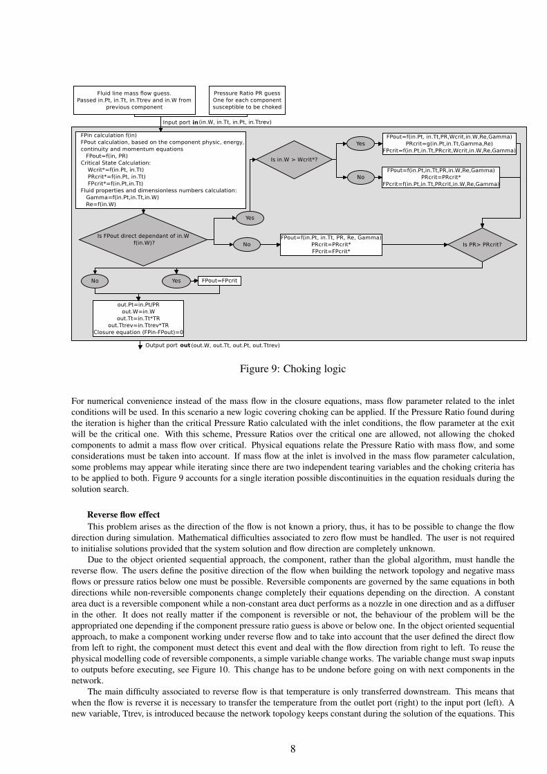
Figure 9: Choking logic

For numerical convenience instead of the mass flow in the closure equations, mass flow parameter related to the inletconditions will be used. In this scenario a new logic covering choking can be applied. If the Pressure Ratio found duringthe iteration is higher than the critical Pressure Ratio calculated with the inlet conditions, the flow parameter at the exitwill be the critical one. With this scheme, Pressure Ratios over the critical one are allowed, not allowing the chokedcomponents to admit a mass flow over critical. Physical equations relate the Pressure Ratio with mass flow, and someconsiderations must be taken into account. If mass flow at the inlet is involved in the mass flow parameter calculation,some problems may appear while iterating since there are two independent tearing variables and the choking criteria hasto be applied to both. Figure 9 accounts for a single iteration possible discontinuities in the equation residuals during thesolution search.

Reverse flow effectThis problem arises as the direction of the flow is not known a priory, thus, it has to be possible to change the flow

direction during simulation. Mathematical difficulties associated to zero flow must be handled. The user is not requiredto initialise solutions provided that the system solution and flow direction are completely unknown.

Due to the object oriented sequential approach, the component, rather than the global algorithm, must handle thereverse flow. The users define the positive direction of the flow when building the network topology and negative massflows or pressure ratios below one must be possible. Reversible components are governed by the same equations in bothdirections while non-reversible components change completely their equations depending on the direction. A constantarea duct is a reversible component while a non-constant area duct performs as a nozzle in one direction and as a diffuserin the other. It does not really matter if the component is reversible or not, the behaviour of the problem will be theappropriated one depending if the component pressure ratio guess is above or below one. In the object oriented sequentialapproach, to make a component working under reverse flow and to take into account that the user defined the direct flowfrom left to right, the component must detect this event and deal with the flow direction from right to left. To reuse thephysical modelling code of reversible components, a simple variable change works. The variable change must swap inputsto outputs before executing, see Figure 10. This change has to be undone before going on with next components in thenetwork.

The main difficulty associated to reverse flow is that temperature is only transferred downstream. This means thatwhen the flow is reverse it is necessary to transfer the temperature from the outlet port (right) to the input port (left). Anew variable, Ttrev, is introduced because the network topology keeps constant during the solution of the equations. This

8

Direct flow Reverse flow Reverse flow and reversible component PR∗= 1PR T R∗= 1

T R

Upstream Pressure in.Pt Upstream Pressure in.PtPR Upstream Pressure in.Pt∗= in.Pt

PRUpstream Temperature in.Tt Upstream Temperature in.Tt ·T R Upstream Temperature in.Tt∗= in.Tt ·T RDownstream Pressure in.Pt

PR Downstream Pressure in.Pt Downstream Pressure out.Pt∗= in.Pt∗PR∗

Downstream Temperature in.Tt ·T R Downstream Temperature in.Tt Downstream Temperature out.Tt∗= in.Tt∗ ·T R∗

Figure 10: Reversible components under reverse flow. Variable change to reuse physical modelling programming

Figure 11: Temperatures discontinuities around PR=1

new variable is calculated through the line in the same way as the the total temperature, multiplying by the componenttemperature ratio (out.Ttrev = in.Ttrev ·T R). In the node where the flow line starts, the temperature for reverse flow istearing variable and the correspondent closure equation is the temperature at the final node. The node at the beginning ofthe line decides to pass the direct or reverse temperature depending on the mass flow sign.

Initialisation and multilevel strategyAs reverse flow must be overcome, the philosophy is to initialise mass flow to zero and components pressure and

temperature ratios to one. The system of equations itself, decides during convergence, the flow direction with the massflow sign. Therefore, the components must deal with zero flow, and for a robust solution, the closure equations must havean appropriate behaviour around mass flow zero (continuity and residual slopes different from zero or infinite). This isnot easy to achieve. For instance, a component between two boundaries may have discontinuities around zero mass flow,Figure 11. In the region next to PR=1, the expression used to calculate the mass flow parameter depends on the flowdirection:

• Direct flow: PR = 1+ ε FPOut = f (in.W,Pinlet ,PR,Ttinlet) = f (in.W,B1.Pt,(1+ ε),B1.Tt)

ε → 0 FPOut = f (in.W,B1.Pt,1,B1.Tt) (5)

• Reverse flow: PR = 1− ε FPOut = f (in.W,Pinlet ,1

PR ,Ttinlet) = f (in.W, B1.Pt(1−ε) ,

1(1−ε) ,B2.Tt)

ε → 0 FPOut = f (in.W,B1.Pt,1,B2.Tt) (6)

B1.Tt is different from B2.Tt around PR=1. To deal with this discontinuity the system is solved in separate levels.Firstly, it is calculated an estimation of the mass flow using B1.Tt in the mass flow parameter expression. This estimationis used as initial value for the second level that uses the correct expression (either 1 or 2 depending on the flow direction).

It is somehow a continuity method, used to solve nonlinear systems of equations by successive approximations to thefinal problem. Although, there are two systems to solve, the procedure accelerates the computation time, provided goodperformance for the easier problem and the solution to initialise the whole problem. The decision of different solvinglevels is taken at the components and library creation. It is a task for component developers, not for final users.

The multilevel strategy is also adequate for more advanced components, where the complexity of the modellingmethodology requires a proper initialisation. More simple levels could solve components and get a choking estimationor the direction of flow and for higher levels would be computed most sophisticated calculations, as some zoomingcapabilities with other program interactions.

Scaling the problemIn the mathematical equations solution, the use of non-dimensional parameters is recommended; if it is not possible,

it is recommended to scale both, the tearing variables and the closure equations. It helps to achieve a well-conditionedsystem of equations. This scaling process is sometimes useful to avoid numerical problems derived from the magnitudeunits.

To scale or reduce the mass flow, a value for each fluid line must be used that will depend on the nature of the differentcomponents in the fluid line. For pressures in the nodes which are used as unknowns a typical pressure value is enough.ISA pressure at sea level is a good value. With this scale, values of pressures over 100 or under 0.01 are not expectedin typical SAS models. This value can also be used to scale the closure equations for pressure equalities at nodes. Fortemperatures and closure equations equalling temperatures, the ISA temperature at sea level is adequate. As expected

9

Figure 12: Node example

temperatures in a Gas Turbine are in the range 150-2000K, the scaled values may vary around 0.1-10. Pressure ratios andtemperature ratios are not needed to be scaled.

For additional unknowns and closure equations the scaling issue must be studied in detail. The objective is to controlthe residual value and slope of the closure equations to improve the system convergence. For example, to solve the chokingeffect, additional equations equalling the mass flow parameter at the component input and output have been used. Theflow parameter is expected to be of order unity and this closure equation is expected to be of unity order. For componentswhose geometry is defined by the area it works but, for some other with additional geometrical data, as pipes with theassociated length, an additional value to scale this closure equation is needed.

SAS nodeThis is one of the most important components. It is detailed because it is in charge of making the network to work.

In Figure 8 node is organised as an abstract component and three components inherit from it, boundary (SASBound),Pressure Node (SASPr) and internal node (SASNode). Nodes are multiple inputs-multiple outputs. This section affectsto all types of nodes although it is focused on the internal node. The missions of the nodes are:

• To balance pressures.

• To satisfy mass flow continuity.

• To satisfy the energy equation.

Figure 12 shows an example of a very basic network with e internal node. There are m boundaries with lines that inputto the node and n lines that output from the node to their respective boundaries. Each line has a component that relatespressure drop with mass flow. From the possible solutions to satisfy the governing equations, the selected one is to keepall the lines independent from the rest at the iteration level, maintaining the same behaviour in all of them . The nodepressure is introduced as tearing variable and, for every input line there is a closure equation that equals the total pressureat the end of the line with the node pressure. The calculated node pressure is passed to every output line. Mass flowcontinuity equation is not used inside the node calculations but it is added as closure equation.

Some other options could be not to have the pressure node as unknown and equal the incoming lines pressure to apreferred one. It is one less unknown and one less equation than the proposed system of equations. On the other hand, oneof the output mass flows could have been function of the other mass flows and the continuity equation would have beenautomatically satisfied in all iterations. The solutions with a preferred line may fail during convergence, due to numericalissues. For example, a node where many lines with big flows and a leakage line that is the preferred line. All the iterationsiteration, the leakage flow is calculated as the sum of the flow in the remaining lines (with the respective sign). A smallquantity as the sum of big quantities may lead to unexpected numerical behaviours.

Inputs and outputs for a node are defined by the user when the network topology is constructed. New concepts are“effective input” and “effective output”, that represent if really flow is entering or not to the node which has to be takeninto account in the thermal balance. “Effective inputs” are inputs with positive mass flow or outputs with negative massflow. “Effective outputs” are outputs with positive mass flow or inputs with negative mass flow. Total enthalpy enteringthe node is calculated with “effective inputs” and the node temperature is passed only to the effective output lines.

Ttnode =∑e f f ective inputs H

∑e f f ective inputs W(7)

10

Unknowns Closure equations

Cd .in.W EQ1 = B2.Pt−Cd .out.PtPtre f

= 0

Cd .in.Ttrev EQ2 = B2.T t−Cd .out.TtrevTtre f

= 0Cd .β EQ3 = FPout −FPin = 0

Figure 13: A simple Cd model

SAS tearing variables and closure equationsDue to chocking and reverse effects it is necessary to introduce tearing variables to relate the inlet with the outlet in

terms of total pressure and temperature:

• Pressure ratio: defined as PR = in.Ptout.Pt (over one in a direct flow condition)

• Temperature ratio: defined as T R = out.Ttin.Tt (over one if heat is added to the component and the flow is direct)

Pressure ratioPressure ratio appears in the mass flow parameter calculation but also in the closure equation to match the pressure at

the end of the line. Figure 13 shows a simple model with its tearing variables and closure equations. If the starting pointto iterate is Cd.PR0 = 1 Newton Raphson estimates for the next iteration Cd.PR1 .

EQ1 = B2.Pt− B1.PtCd.PR

= 0dEQ1dPR

∣∣∣∣PR=1

= B1.Pt Cd.PR1 = 2− B2.PtB1.Pt

(8)

For values of B2.Pt > 2B1.Pt the first Newton Raphson step tries negative pressure ratios. This effect is caused bythe pressure ratio definition. If the tearing variable is the inverse pressure ratio this problem disappears:

Cd.β =1

Cd.PR=

Cd1.out.PtCd2.in.Pt

EQ1 = B2.Pt−B1.Pt ∗Cd.β = 0dEQ1

dβ

∣∣∣∣β=1

=−B1.Pt Cd.β1 =B2.PtB1.Pt

(9)

According to this, although the PR parameter is maintained in all the component equations, the external tearingvariable to iterate will be β = 1

PR . The variable change is done before executing each component and undone before goingon with next components.

Temperature ratioIf a fixed quantity of heat is added to the example of Figure 13 a new closure equation has to be added to calculate

the temperature ratio TR:

EQ2 =Cd.in.W ∗ c̄p∗Cd.in.Tt ∗ (Cd.T R−1)−Qadded = 0dEQ2dT R

∣∣∣∣T R=1

=Cd.in.W ∗ c̄p∗Cd.in.Tt (10)

Cd.T R1 = 1+Qadded

Cd.in.W ∗ c̄p∗Cd.in.Tt(11)

For high values of Qadded combined with reverse flows, the first Newton Raphson step in the second level triesnegative temperature ratios which lead to negative values of out.Tt and the consequent convergence failure.

Cd.out.Tt1 =Cd.in.Tt1 ·Cd.T R1→ reverse f low→Cd.out.Tt1 =Cd.in.Ttrev1 ·Cd.T R1 (12)

This effect disappears if instead of the temperature ratio as tearing, Cd.∆T is used instead:

Cd.∆T =Cd.out.Tt−Cd.in.Tt

Tre f= (Cd.T R−1) · Cd.in.Tt

Tre f

A negative value of TR implies also a negative value of ∆T but now it does not imply a negative value of out.Tt.

Cd.out.Tt1 = Tre f ·Cd.∆T1 +Cd.in.Ttrev1

11

Although ∆T is negative the reverse temperature tries to make out.Tt positive.This variable change is introduced in the same way as the one in the pressure ratio parameter, before entering the

component and undone after the execution.

SAS Network Summary• For a given network topology, representing a model, the incidence matrix can be constructed, closed loops can be

detected and opened. The network can be sorted, to be executed in an appropriate order, bet keeping the topologydefined.

• The nodes, including boundaries will contribute to build the system equations to be solved. For each output linethe mass flow and reverse temperature will be added as tearing variables, mass flow to be solved in a lower levelthan reverse temperature. For the input lines two closure equations will be added, pressure balance in the lowerlevel and temperature balance in the higher. Each node, not boundary, will add the total pressure as tearing variableand mass flow as closure equation in the lower level.

• For each component susceptible to be choked and reversed, the inverse pressure ratio will be added as tearingvariable in the lower level and temperature difference (if necessary) in the higher level. Continuity of flows willbe added as closure equation in the lower level

(FPout−FPin

FPscale= 0)

. Energy balance must be imposed at higher levelusing the scaled ∆T as tearing.

• Lower level solution starts iterating the tearing variables to match the closure equations. In all iterations, forgiven values of the unknowns, the network is executed in the right order and closure equations residues are thencalculated.

• The lower level is solved. Keeping the results from the lower level, the higher levels are executed. Zooming andmore accurate calculations will be added to higher levels of execution. It is possible to include design options byadding proper tearing variables and closure equations after the higher level of the network.

CONCLUSIONS• An approach to network models solution is described. Advantages and disadvantages compared to different ap-

proaches have been taken into account. Some of the issues found in Gas Turbine SAS models have been used asexample.

• Some of the most important mathematical difficulties have been arisen and a solution is proposed for them. Aclear understanding of the problem details helps to find an adequate solution. Although further details as ingestionor some other complex components could be explained, the essential is showed in this paper.

• There are better and worse mathematical approaches to overcome the problem. This issue has been discussed andthe approach presented in this work provides a robust solution. The resultant systems of nonlinear equations maybe solved with the Newton Raphson method.

REFERENCES1. ESDU Fluid Mechanics, Internal Flow, www.esdu.com

2. I. S. Duff , J. K. Reid, An Implementation of Tarjan’s Algorithm for the Block Triangularization of a Matrix, ACMTransactions on Mathematical Software (TOMS), v.4 n.2, p.137-147, June 1978.

3. M. Shacham, S. Macchietto, L. F. Stutzman and P. Babcock, Review, Equation Oriented Approach To ProcessFlowsheeting, Computers & Chemical Engineering, Vol 6, No.2, pp. 79-95, 1982.

4. P. P. Walsh, P. Fletcher, Gas Turbine Performance, second edition, Blackwell Publishing, chapters 5, 6 and 7.

12