comparative study of transient and quasi …etd.lib.metu.edu.tr/upload/12617006/index.pdf ·...

COMPARATIVE STUDY OF TRANSIENT AND QUASI-STEADY

AEROELASTIC ANALYSIS OF COMPOSITE WIND TURBINE BLADE

IN STEADY WIND CONDITIONS

A THESIS SUBMITTED TO

THE GRADUATE SCHOOL OF NATURAL AND APPLIED SCIENCES

OF

MIDDLE EAST TECHNICAL UNIVERSITY

BY

HAKAN SARGIN

IN PARTIAL FULFILLMENT OF THE REQUIREMENTS

FOR

THE DEGREE OF MASTER OF SCIENCE

IN

AEROSPACE ENGINEERING

FEBRUARY 2014

Approval of the thesis:




submitted by HAKAN SARGIN in partial fulfillment of the requirements for the

degree of Master of Science in Aerospace Engineering Department, Middle East

Technical University by,

Prof. Dr. Canan Özgen _____________________

Dean, Graduate School of Natural and Applied Sciences

Prof. Dr. Ozan Tekinalp _____________________

Head of Department, Aerospace Engineering

Prof. Dr. Altan Kayran _____________________

Supervisor, Aerospace Engineering Dept., METU

Examining Committee Members:

Prof. Dr. Yavuz Yaman _____________________

Aerospace Engineering Dept., METU

Prof. Dr. Altan Kayran _____________________


Assoc. Prof. Dr. Melin Şahin _____________________


Assoc. Prof. Dr. Nilay Sezer Uzol _____________________


Murat Günel, M.Sc. _____________________

Turkish Aviation Industry, TAI

Date: 07.02.2014

I hereby declare that all information in this document has been obtained and

presented in accordance with academic rules and ethical conduct. I also declare

that, as required by these rules and conduct, I have fully cited and referenced

all material and results that are not original to this work.

Name, Last name: Hakan Sargın

Signature :

iv

v

ABSTRACT




SARGIN, Hakan

M.S., Department of Aerospace Engineering

Supervisor: Prof. Dr. ALTAN KAYRAN

February 2014, 143 Pages

The objective of this study is to conduct a comparative study of the transient and

quasi-steady aeroelastic analysis of a composite wind turbine blade in steady wind

conditions. Transient analysis of the wind turbine blade is performed by the multi-

body dynamic code Samcef Wind Turbine which uses blade element momentum

theory for aerodynamic load calculation. For this purpose, a multi-body wind turbine

model is generated with rigid components except for the turbine blades. For the

purposes of the study, a reference three dimensional blade is designed using inverse

design methodology. Dynamic superelement of the turbine blades are created and

introduced into multi-body model of the wind turbine system, and transient

aeroelastic analysis of the multi-body wind turbine system is performed in steady

wind conditions. As a follow-up study, quasi-steady aeroelastic analysis of the same

composite wind turbine blade is performed by coupling a structural finite element

solver with an aerodynamic tool based on blade element momentum theory. Quasi-

vi

steady aeroelastic analysis of the blade is performed at different azimuthal positions

of the blade and transient effects due to the rotation of the blade are ignored. The

article aims at investigating the applicability of quasi-steady aeroelastic modeling of

the turbine blade in steady wind conditions by comparing the deformations obtained

by quasi-steady aeroelastic analysis and transient aeroelastic analysis of the complete

turbine system at the same azimuthal positions of the blade. The presented results

conclude that the quasi-steady aeroelastic analysis and transient aeroelastic analysis

have a close match and the coupling between the finite element solver with a blade

element momentum based aerodynamic tool can be used for static aeroelastic

analysis at preliminary design state of a composite wind turbine blade.

Keywords: Aeroelasticity, Composite Wind Turbine Blade, Finite Element Analysis,

Blade Element Momentum Theory, FEM-BEM Coupling.

vii

ÖZ

KOMPOZİT RÜZGÂR TÜRBİN KANADININ SABİT RÜZGÂR

KOŞULLARINDA ZAMANA BAĞLI VE NEREDEYSE STATİK

AEROELASTİK ANALİZLERİNİN KARŞILAŞTIRMALI ÇALIŞMASI

SARGIN, Hakan

Yüksek Lisans Havacılık ve Uzay Mühendisliği Bölümü

Tez Yöneticisi: Prof. Dr. ALTAN KAYRAN

Şubat 2014, 143 Sayfa

Bu tezin konusu, kompozit rüzgâr türbin kanadının sabit rüzgâr koşullarında zamana

bağlı ve neredeyse statik aeroelastik analizlerinin karşılaştırılmalı çalışılmasıdır.

Rüzgâr kanadının zamana bağlı analizleri, aerodinamik analizler için pal elemanı

momentum teorisini kullanan çok parçalı dinamik kodlu Samcef Wind Turbine

kullanılarak yapılmıştır. Bu amaçla, türbin kanatları haricindeki bileşenler esnemez

olacak şekilde çok parçalı rüzgâr türbin modeli yaratılmıştır. Rotor kanadı içinse, üç

boyutlu referans kanat tersine tasarım metodu uygulanarak tasarlanmıştır. Dinamik

supereleman türbin kanatları yaratılmış ve çok parçalı rüzgâr türbini modeline

tanıtılmış ve sabit rüzgâr koşullarında çok parçalı rüzgâr türbininin zamana bağlı

aeroelastik analizleri yapılmıştır. Bu çalışmanın devamı olarak, aynı kompozit rüzgâr

türbini kanadının neredeyse statik analizleri, bir yapısal sonlu eleman çözücüsü ile

pal elemanı momentum teorisi temelli aerodinamik bir araç eşleştirilerek yapılmıştır.

viii

Neredeyse statik aeroelastik analizler, kanadın farklı ufuk açılarında ve dönüşten

kaynaklanan etkiler yok sayılarak yapılmıştır. Çalışma, kanadın aynı ufuk açılarında

neredeyse statik aeroelastik rüzgâr kanadı modelinin analizleri sonucunda elde edilen

deformasyonlar ile bütün türbin sisteminin zamana bağlı aeroelastik analizleri

sonucunda elde edilen deformasyonları karşılaştırarak uygulanabilirliğini araştırmayı

amaçlamaktadır. Sunulan sonuçlar, neredeyse statik aeroelastik analizler ile zamana

bağlı aeroelastik analizlerin yakın olarak eşleştiğini göstermektedir ve tasarım

aşamasındaki kompozit rüzgâr türbinin statik aeroelastik analizleri için yapısal sonlu

eleman çözücüsünün pal elemanı momentum teorisi temelli aerodinamik bir araç ile

eşleşmesi kullanılabilir.

Anahtar Kelimeler: Aeroelastikiyet, Kompozit Rüzgâr Türbin Kanadı, Sonlu Eleman

Analizleri, Pal Elemanı Momentum Teorisi, SEA-PEM Eşleştirmesi.

ix

To My Family

x

ACKNOWLEDGMENTS

I would like to thank my supervisor Prof. Dr. Altan Kayran for his guidance, support,

encouragement and patience throughout the study. The comments of the examining

committee members are also greatly acknowledged.

I want to thank my colleagues Erdoğan Tolga İnsuyu, Levent Ünlüsoy and Evren

Sakarya for their assistance and collaboration in the study.

I would also gratefully appreciate the support and assistance of all my cherished

friends but especially Mehmet Ozan Gözcü for his assistance.

I would like to thank my parents for their guidance and insight and wife for their care

and support.

xi

TABLE OF CONTENTS

ABSTRACT ................................................................................................................ v

ÖZ .............................................................................................................................. vii

ACKNOWLEDGMENTS ........................................................................................... x

TABLE OF CONTENTS ............................................................................................ xi

LIST OF TABLES .................................................................................................... xiii

LIST OF FIGURES ................................................................................................... xv

LIST OF SYMBOLS ................................................................................................ xix

LIST OF ABBREVIATIONS ................................................................................... xxi

CHAPTERS

1.INTRODUCTION .................................................................................................... 1

1.1 Historical Review and Wind Energy ............................................................. 4

1.1.1 Windmills ................................................................................................ 5

1.1.2 European Horizontal Axis Windmills ..................................................... 7

1.1.3 Wind Turbines ........................................................................................ 9

1.2 General Description and Layout of a Wind Turbine ................................... 12

1.2.1 Vertical Axis Wind Turbines ................................................................ 13

1.2.2 Horizontal Axis Wind Turbines ............................................................ 15

1.2.3 Layout of a Horizontal Axis Wind Turbine .......................................... 15

1.3 Literature Review......................................................................................... 20

1.4 Scope of the Thesis ...................................................................................... 23

2.ROTOR AERODYNAMICS .................................................................................. 25

2.1 The Actuator Disc Model (One-Dimensional Linear Momentum Theory) . 25

2.2 Rotor Disc Theory (Angular Momentum Theory) ....................................... 28

2.3 The Blade Element Momentum (BEM) Theory .......................................... 31

xii

3.INVERSE DESIGN OF THE REFERENCE BLADE AND QUASI-STEADY

AEROELASTIC ANALYSIS OF THE WIND TURBINE BLADE ........................ 41

3.1 Selection of Composite Materials for the Blade .......................................... 43

3.2 Variational Asymptotic Beam Section Analysis; PreVABS and VABS ..... 46

3.3 VABS Modeling of the Wind Turbine Blade .............................................. 53

3.4 Finite Element Modeling of the Wind Turbine Blade ................................. 56

3.4.1 Geometric Modeling ............................................................................. 56

3.4.2 Mesh Generation and Property Assignment ......................................... 58

3.4.3 Application of the Boundary Conditions and Modal Analysis ............. 61

3.5 Quasi-steady Aeroelastic Analysis ............................................................... 64

3.5.1 Results of Quasi-steady Aeroelastic Analysis for Concentrated Load

Cases ..................................................................................................... 68

3.5.2 Results of Quasi-steady Aeroelastic Analysis for Distributed Load

Cases ..................................................................................................... 76

4.MULTI-BODY MODELING of the REFERENCE TURBINE AND TRANSIENT

AEROELASTIC ANALYSIS OF THE BLADE ....................................................... 81

4.1 Generation of Superelement Blade .............................................................. 82

4.2 Wind Turbine Modeling in Samcef Wind Turbine ...................................... 89

4.3 Results of the Transient Aeroelastic Analysis ............................................. 95

5.CONCLUSION ..................................................................................................... 103

REFERENCES ......................................................................................................... 107

A.PREVABS INPUT FILES ................................................................................ 115

B.WT_PERF INPUT FILE .................................................................................. 127

C.AERODYNAMIC COEFFICIENTS of NREL BLADE ................................. 135

D.SAMCEF AERODYNAMIC VALIDATION ................................................. 139

xiii

LIST OF TABLES

TABLES

Table 3.1 Chord and Twist Distributions of NREL Phase VI Blade [41].................. 42

Table 3.2 Physical and Mechanical Properties of Prepreg Hybrid Carbon/Fiberglass

Composite Triax, 70% 0° Unidirectional Type [27] .................................................. 45

Table 3.3 Physical and Mechanical Properties of E-Glass Harness Satin Weave

Fabric 7781/EA93 [27] .............................................................................................. 46

Table 3.4 Sectional Beam Properties of UAE Phase VI Blades [41]......................... 53

Table 3.5 Sectional Beam Properties of the Inverse Designed Reference Blade....... 54

Table 3.6 Sectional Ply Numbers and Thickness Variation ....................................... 56

Table 3.7 Number of Elements and Nodes Used in the Detailed Finite Element

Model of the Inverse Design Blade ............................................................................ 59

Table 3.8 Summary of Center of Gravity, Principal Inertias, Radii of Gyration, Mass

and Volume of the Inverse Design Blade .................................................................. 60

Table 3.9 Global Mode Shapes and Natural Frequency Results of the Inverse Design

Blade .......................................................................................................................... 64

Table 3.10 Results of Quasi-steady Aeroelastic Analysis for Concentrated Loads ... 76

Table 3.11 Incremental Changes in Angle of Attack Values with the Iteration

Numbers (Azimuthal Position - 90 Degree) .............................................................. 79

Table 3.12 Results of Quasi-steady Aeroelastic Analysis for Distributed Loads ...... 79

Table 4.1 Comparison of the Natural Frequencies..................................................... 87

Table 4.2 Tower Properties Used in the Multi-body Simulation of the Wind Turbine

System ........................................................................................................................ 91

Table 4.3 Blade Properties Used in the Multi-body Simulation of the Wind Turbine

System ........................................................................................................................ 92

xiv

Table 4.4 Samtech Controller & Fast Drive Train Properties in the Multi-body

Simulation of the Wind Turbine System .................................................................... 92

Table 4.5 Constant Function Table defined in Multi-body Dynamic Model of the

Wind Turbine System ................................................................................................. 94

Table 4.6 Rated Load Case defined in Multi-body Dynamic Model of the Wind

Turbine System .......................................................................................................... 95

Table 4.7 Axial and Tangential Tip Displacement Variations at Different Azimuthal

Positions ................................................................................................................... 100

Table 4.8 Comparison of the Tip Deflection Results ............................................... 100

Table 4.9 Flapwise Bending Moments at r=0.66 m Calculated for the Constant Wind

Speed (15 m/s). ......................................................................................................... 101

xv

LIST OF FIGURES

FIGURES

Figure 1.1 The Worldwide Wind Capacity by the end of 2013 [4] ............................. 2

Figure 1.2 Total Installed Capacity for Market Leaders by the end of June 2013 [4] . 2

Figure 1.3 Growth in Size of Commercial Wind Turbine Designs [7] ........................ 3

Figure 1.4 The Earliest Evidence from Iconography of Around 2450 B.C. Shows

Wind Powered Ship [24] .............................................................................................. 4

Figure 1.5 A Diagram of Heron’s Organ, 1st Century [11] .......................................... 5

Figure 1.6 Ancient Persian Vertical Axis Windmills [51] ........................................... 6

Figure 1.7 The Vertical-axis Chinese Windmill, With Eight Junk Sails [14].............. 7

Figure 1.8 A Picture of Windmill from an English Prayer-book “Windmill Psalter” of

1270 [2] ........................................................................................................................ 8

Figure 1.9 Cog and Gear Design and Post Windmill [3] ............................................. 8

Figure 1.10 In 1888 Charles F. Brush Invented the First Automatically Operated

Horizontal Axis Wind Turbine [49] ........................................................................... 10

Figure 1.11 La Cour’s First Electricity Producing Wind Turbine in 1891, Askov,

Denmark [1] ............................................................................................................... 11

Figure 1.12 Modern Offshore Wind Turbine [32] ..................................................... 12

Figure 1.13 Wind Turbine Types [20] ....................................................................... 13

Figure 1.14 Several Types of VAWTs [10] ............................................................... 14

Figure 1.15 Typical Horizontal Axis Wind Turbine Blade [18] ................................ 16

Figure 1.16 Rotating Pitch Mechanism Attached to the Hub [19] ............................. 17

Figure 1.17 Hub Types [6] ......................................................................................... 18

Figure 1.18 Schematic View of HAWT Drive Train [12] ......................................... 18

Figure 1.19 Yaw Drive Mechanism [19] ................................................................... 19

Figure 1.20 Complete Wind Turbine System with Tower and Foundation [6] ......... 20

xvi

Figure 2.1 Discontinuous Pressure Drop across the Rotor [23] ................................. 26

Figure 2.2 Airflow Rotates in the Opposite Direction behind the Downwind Turbine

Rotor [24] ................................................................................................................... 28

Figure 2.3 Extended Momentum Theory, Taking into Consideration the Rotating

Rotor Wake [19] ......................................................................................................... 29

Figure 2.4 Schematic of the Rotor Disk Theory [23] ................................................. 30

Figure 2.5 Local Blade Element Velocities and Aerodynamic forces [26] ............... 32

Figure 2.6 Normal and Tangential Force Distribution over the Blade [19] ............... 34

Figure 2.7 Tip Loss Flow Diagram and Azithimuthal Variation at Various Radial

Positions of the Blade [23, 30] ................................................................................... 37

Figure 3.1 Geometric Presentation of the Wing Studied [15] .................................... 42

Figure 3.2 Chord and Twist Distribution of the NREL Blade ................................... 43

Figure 3.3 Structure, Spar Location and Materials used in the Different Parts of the

Blade [27] ................................................................................................................... 45

Figure 3.4 Schematic Representation of an Airfoil Profile in PreVABS [15] ........... 47

Figure 3.5 Segmented Blade Cross-Section Definitions for PreVABS [15] .............. 48

Figure 3.6 PreVABS Modeling of NREL Blade Section. (a) Dimensionalized Cross-

section Profile of the NREL Inverse Design Blade (b) High Resolution Finite

Element Mesh on the Cross-section of the Blade (c) Zoomed View of the Spar-Skin

Connection (d) Zoomed View High Resolution Finite Element Mesh at the Trailing

Edge ............................................................................................................................ 49

Figure 3.7 VABS - PreVABS Coupling Flow Chart and Decomposition of a Three-

Dimensional Blade into Two-Dimensional Cross-section and a One-Dimensional

Beam [25] ................................................................................................................... 50

Figure 3.8 Comparison of the Variation of the Flapwise Bending Stiffness of the

NREL Blade and the Inverse Design Blade ............................................................... 55

Figure 3.9 Isometric View of the Skin Surfaces at the Root and the Transition Part of

the Blade ..................................................................................................................... 57

Figure 3.10 Cross-Sectional View of the Finite Element Mesh of the Front and Rear

Part of the Skin of the Blade ...................................................................................... 57

Figure 3.11 Isometric View of the Spar Location of the Blade ................................. 58

xvii

Figure 3.12 Finite Element Mesh of the NREL Blade ............................................... 59

Figure 3.13 Fiber Orientation and Material Assignment ........................................... 60

Figure 3.14 Zoomed View of Fixed Root Nodes in MSC®/PATRAN ..................... 61

Figure 3.15 1st Flapwise Bending Mode Shape of the Inverse Design Blade ............ 62

Figure 3.16 1st Edgewise Bending Mode Shape of Inverse Design Blade................. 62

Figure 3.17 2nd

Flapwise Bending Mode Shape of the Inverse Design Blade ........... 63

Figure 3.18 Torsional Mode Shape of the Inverse Design Blade [24.52 Hz] ............ 63

Figure 3.19 Flow Chart of the Coupling Procedure [43] ........................................... 65

Figure 3.20 Lift Force Coefficient Data of the NREL S809 Airfoil [41] .................. 66

Figure 3.21 Drag Force Coefficient Data of NREL S809 Airfoil [41] ...................... 67

Figure 3.22 NREL S809 Airfoil – Extrapolated Aerodynamic Force Coefficients ... 68

Figure 3.23 Azimuth Positions of the NREL Blade ................................................... 69

Figure 3.24 Axial and Tangential Induction Factor Variations of NREL S809 ........ 70

Figure 3.25 In-flow Angle and Angle of Attack Variations of the NREL S809 Blade -

Azimuth 0 ................................................................................................................... 71

Figure 3.26 Normal and Tangential Force Variations of NREL S809 Airfoil –

Azimuth 0 ................................................................................................................... 71

Figure 3.27 Location of Aerodynamic Force Application Nodes and Loads Applied

to the Inverse Design Blade for Flapwise Deflection Calculation ............................. 72

Figure 3.28 Blade Deflection at 72 rpm and 15m/s Wind Speed – After the 1st

Iteration ...................................................................................................................... 73

Figure 3.29 Deformed Blade and Shifted Node Locations ........................................ 74

Figure 3.30 Blade Deflection at 72 rpm and 15m/s Wind Speed – After the 2nd

Iteration ...................................................................................................................... 74

Figure 3.31 Blade Deflection at 72 rpm and 15m/s Wind Speed – After the 3rd

Iteration ...................................................................................................................... 75

Figure 3.32 RBE3 Elements and Distribution of the Aerodynamic Loads Applied at

the Aerodynamic Center to Upper Section Nodes ..................................................... 77

Figure 3.33 Flapwise Deflection at 72 rpm and 15m/s Wind Speed – After the 1st

Iteration ...................................................................................................................... 78

Figure 4.1 Isometric View of the Blade Geometry in Samcef Field .......................... 84

xviii

Figure 4.2 Generation of the Retained Nodes and Mean Elements ........................... 85

Figure 4.3 Isometric View of the Meshed Blade ....................................................... 86

Figure 4.4 1st Flapwise Bending Mode Shape of the Superelement Blade Model

[4.13 Hz] ..................................................................................................................... 88

Figure 4.5 1st Edgewise Bending Mode Shape of the Superelement Blade Model ... 88

Figure 4.6 2nd Flapwise Bending Mode Shape of the Superelement Blade Model

[17.52 Hz] ................................................................................................................... 89

Figure 4.7 Torsional Mode Shape of the Superelement Blade Model [28.40 Hz] ..... 89

Figure 4.8 Multi-body Model of the Wind Turbine Parts [55] .................................. 90

Figure 4.9 Multi-body Dynamic Model of the Wind Turbine System ....................... 93

Figure 4.10 Assignment of the Aerodynamic Coefficients to Multi-body Dynamic

Model of the Wind Turbine System ........................................................................... 93

Figure 4.11 Assignment of the Constant Function to Control Node .......................... 94

Figure 4.12 Advanced Aero Options for Transient Analysis ..................................... 95

Figure 4.13 Normal Force Variation across the Blade for Different Azimuthal

Positions ..................................................................................................................... 96

Figure 4.14 Tangential Force Variation across the Blade for Different Azimuthal

Positions ..................................................................................................................... 97

Figure 4.15 Moment Variation across the Blade for Different Azimuthal Positions . 97

Figure 4.16 Axial Tip Displacement of the Blade towards Downwind ..................... 98

Figure 4.17 Tangential Tip Displacement of the Blade towards Next Blade ............ 98

Figure A.1 Schematic of VABS CoordinatesSystem...............................................115

Figure B.1 WT_Perf Output File..............................................................................130

Figure D.1 Aerodynamic Input File Sample for SWT..............................................139

Figure D.2 Assignment of the Aerodynamic Coefficients to Multi-body Dynamic

Model........................................................................................................................141

Figure D.3 Imposition of Rotor Speed Boundary Condition in SWT .....................141

Figure D.4 Imposition of Pitch Angle Boundary Condition in SWT ......................142

Figure D.5 Initial Static Computation Option...........................................................143

xix

LIST OF SYMBOLS

Angle of Attack

Angle of Relative Wind

Angular Induction Factor

Angular Velocity of the Rotor

Axial Induction Factor

Chord Length

Combined tip-loss and hub-loss coefficient

Density of Air

Differential Thrust

Differential Torque

Drag Coefficient

Drag Force

Lift Coefficient

Lift Force

Local Angular Velocity of the Flow

Local Tip Speed Ratio

Mass Center of the Cross-section

Mass Flow Rate

Mass Moment of Inertia

Mass per Unit Span

Moment Coefficient

Normal Force

N Number of Blades

Pitch Axis Location of the Section in X Coordinate Frame

Pitch Axis Location of the Section in Y Coordinate Frame

xx

Pitching Moment

Poison’s Ratio

Position for Web Centers in X Coordinate Frame

Position for Web Centers in Y Coordinate Frame

Power

Power Coefficient

Prandtl’s Tip-loss Correction

Prandtl’s Hub-loss Correction

Radius

Relative Wind Velocity

Reynolds Number

Rotor Area

Rotor Torque

Shear Modulus of Elasticity

S Stiffness Matrix

Solidity

Section Pitch Angle

Section Twist Angle

Tangential Force

Thrust Coefficient

Thrust Force

Wind Velocity

Young’s Modulus

3-D strain field

xxi

LIST OF ABBREVIATIONS

0-D Dimensionless

1-D One Dimensional

2-D Two Dimensional

3-D Three Dimensional

BEM Blade Element Momentum

CAD Computer Aided Design

CFD Computational Fluid Dynamics

DOFs Degree of Freedoms

DTU Delft University of Technology

EGWF E-Glass Woven Fabric

FE Finite Element

FEM Finite Element Method

GRFP Glass-Fiber Reinforced Plastic

HAWT Horizontal Axis Wind Turbine

HPS High Pressure Surface

LE Leading Edge

LPS Low Pressure Surface

MBD Multi-body Dynamics

MPC Multi-point Constraints

NREL National Renewable Energy Laboratory

OSU Ohio State University

RBE Rigid Body Element

SWT Samcef for Wind Turbine

TE Trailing Edge

UDCF Uni-directional Carbon Fiber

xxii

VAM Variational Asymptotic Methods

VAWT Vertical Axis Wind Turbine

1

CHAPTER 1

INTRODUCTION

The industrial revolution and the increase of the population of the World have

triggered the energy need. The energy consumption in the World has been increasing

rapidly and consecutively energy demand has increased significantly. Generally,

fossil fuels have been used to provide the required energy demand. However, the

depletion of the non-renewable resources and the increasing energy demand of the

world together forced engineers to search for alternative energy resources such as

wind energy. Unlike the stored energy resources such as fossil fuels, coal and natural

gas, renewable energy sources are not depletable. Moreover, renewable energy

sources such as radiation, wind, hydro, solar and thermal offer many benefits. Unlike

the fossil fuel that emits gases that are harmful to environment, renewable energy

resources are clean and do not generate atmospheric contaminants. Renewable

sources might also cost effective depending on the application. When many

considerations are taken account, renewable energy sources became more and more

popular as the alternative energy resource.

Among the renewable energy sources, wind energy is one of the prime resource and

possible candidate to replace the non-renewable energy resources in the future. It

should be noted that power that exists in the wind can be converted into a useful

energy by the wind turbine technology. Cost effective electrical energy, without the

greenhouse effect, can be generated with the wind energy unlike the conventional

energy resources of today which are primarily fossil fuel origin. Furthermore, wind

turbine installation and electricity production costs are lower than or at the worst

2

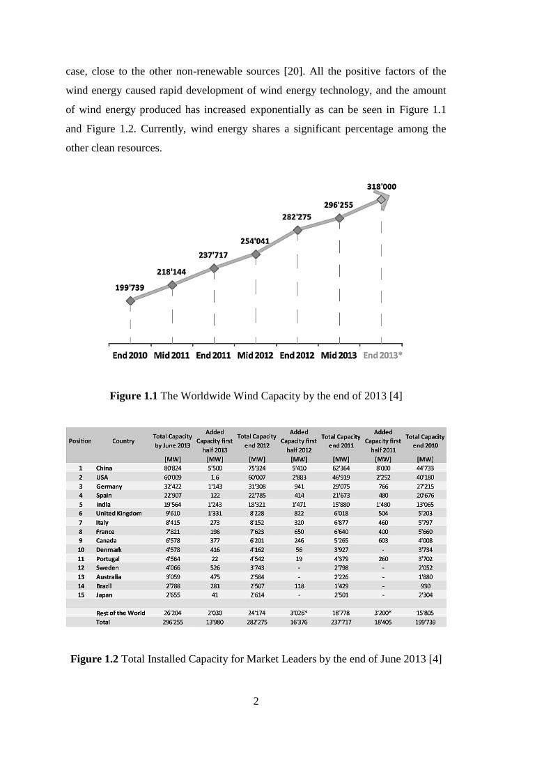
case, close to the other non-renewable sources [20]. All the positive factors of the

wind energy caused rapid development of wind energy technology, and the amount

of wind energy produced has increased exponentially as can be seen in Figure 1.1

and Figure 1.2. Currently, wind energy shares a significant percentage among the

other clean resources.

Figure 1.1 The Worldwide Wind Capacity by the end of 2013 [4]

Figure 1.2 Total Installed Capacity for Market Leaders by the end of June 2013 [4]

3

As mentioned earlier, wind turbine technology is rapidly evolving technological area

and although significant developments have taken place over the last 30 years, wind

turbine technology still has to be improved further to meet the challenges of the next

generation wind turbine systems. To enhance the energy capture and reduce the cost

of the generated electricity, wind turbines have been getting larger and larger [21]. In

the 1980s, an average wind turbine had approximately 10-15 m diameter and

produced almost 50 kW while the current wind turbines have 150 m rotor diameter

and have an energy extraction capacity of almost 7-8 MW [22]. Figure 1.3 shows the

growth in size of commercial wind turbine designs.

Figure 1.3 Growth in Size of Commercial Wind Turbine Designs [7]

However, building very large machines introduce new problems in the practical

design and cause stability issues which should be overcome to obtain reliable

designs. For this purpose, geometric nonlinearities and aeroelastic instability issues

need to be accurately accounted for in the design process of the wind turbine system.

Aeroelastic effects can significantly change the aerodynamic load distribution

especially in long turbine blades which are more flexible compared to small turbine

4

blades. For accurate estimation of the loads acting on the turbine blade, flexibility of

the blade has to be taken into consideration in the design process. Today,

aeroelasticity has become a key issue in the development process of long-lasting,

flexible, large wind turbines. To achieve this goal, it is important to investigate

aeroelastic effects in wind turbines and use reliable aeroelastic tools in the design

process to avoid the failure, and estimate the loads accurately.

1.1 Historical Review and Wind Energy

Harnessing the energy from the wind power is not a new concept. Through the ages,

wind energy has been used for different purposes and the first example of wind

power usage in history was started with the sail boats. Approximately at 4000 B.C.,

the ancient Chinese and Egyptians were recorded as the first who had learned to use

the wind power at their primitive rafts. They attached cotton-made sails to the long

narrow boards to use the power of wind for powered transportation [5]. Figure 1.4

shows an example of the wind powered ship from the earliest evidence of

iconography of around 2450 B.C. [24].

Figure 1.4 The Earliest Evidence from Iconography of Around 2450 B.C. Shows

Wind Powered Ship [24]

5

The first written evidence for converting the wind energy into useful mechanical

power was found in ancient Greece. Heron of Alexandria (Heron Alexandrinus (10-

85 A.D.)) is one of the greatest mathematician and engineer of the ancient world and

best known as the first person who used wind power in his inventions [45]. He

invented the Heron’s organ which was creating sounds “like the sound of flute”. This

machine had a wind wheel which was connected to a piston. As the wind wheel

turned in the wind, the piston started to raise and descend. With this movement, the

compressed air in the pistons went out from cylindrical tubes and this was creating

the sound as illustrated in Figure 1.5. This device is believed to be the first example

of wind powering machine.

Figure 1.5 A Diagram of Heron’s Organ, 1st Century [11]

1.1.1 Windmills

Another ancient use for wind energy was in the form of windmills. According to

verbal records which are not reliable as written sources, wind power for mechanical

6

use started with Babylonian emperor Hammurabi who used windmills for irrigation

in 1700 B.C. [9]. However, for most of the historians, the earliest vertical axis

windmill was designed for agricultural activities, such as water pumping and grain

grounding, around 500-900 A.D. in Sistan at ancient Persia [12]. Figure 1.6 shows

the ancient Persian vertical axis windmill used for grain grounding.

Figure 1.6 Ancient Persian Vertical Axis Windmills [51]

The first Persian windmills were composed of two main parts. First component was

vertical shaft fitted with sails or rectangle shape blades in order to catch the wind.

Second one was the grinding stone which was directly driven by the wind-wheel.

The windmills were structurally built to increase the wind velocity entering the

windmill field. The apertures at the front face were placed narrower than the rear side

and the directions of the apertures were oriented by the north-south direction of the

120 day winds [33]. As a consequence, these windmills were wind direction

dependent devices.

Like in Persia, China is one of the pioneers for windmill usage. The mural paintings

at “Sandaohao” [23] have shown the images that evidencing the use of vertical axis

7

windmills in China for at least approximately 1800 years. Unlike the Persian mills,

Chinese wind driven devices were wind direction independent like modern vertical

axis wind turbines. An example of the vertical-axis Chinese Windmill with eight

junk sails is given in Figure 1.7.

Figure 1.7 The Vertical-axis Chinese Windmill, With Eight Junk Sails [14]

1.1.2 European Horizontal Axis Windmills

Europeans started to use windmills later than Persians and Chinese. However, apart

from the Eastern civilizations, they tried to convert the power of wind to mechanical

energy by horizontal axis windmills. There are lots of speculations about the

invention of horizontal axis windmills, but according to historians, at the end of 12th

century, the horizontal axis windmills were invented and started to be used in

Northwestern Europe [10]. In Figure 1.8, a picture of windmill from 13th

century is

shown.

8

Figure 1.8 A Picture of Windmill from an English Prayer-book “Windmill Psalter”

of 1270 [2]

Early designs were adopted from water wheel and were named as “Post Windmills”.

These wind devices had four blades which were set at an angle and were mounted

directly on a horizontal shaft. When the blades started to run, cog and ring gears

provided the power transmission from horizontal shaft to vertical shaft to turn a

grindstone. An early structural and mechanical design of a Post Windmill is

illustrated in Figure 1.9.

Figure 1.9 Cog and Gear Design and Post Windmill [3]

9

Since the invention of Post Windmill, the design techniques are improved and many

types of windmills had been developed and have been used all over the Europe.

Smock mill, Dutch mill (Tower mill), and Fan mill are some examples that are still

being used.

1.1.3 Wind Turbines

With the changing demands and improvements on the technology, windmills were

evolved to wind turbines in time. In contrast to a windmill, which is a machine that

converts the wind power into mechanical power for water pumping and grain

grinding, a wind turbine converts the wind energy to electrical energy [6]. The first

wind turbine was invented by Professor James Blyth of Anderson’s College,

Glasgow in 1887. Blyth had constructed a 10-meter-high; cloth-sailed wind turbine

to light his home, and this was accepted as the first successful attempt in electricity

generation through wind power. In the winter of 1888, another pioneer Charles Brush

built his own design. The horizontal axis wind turbine of Brush had a rotor diameter

of 17 m and 144 wooden blades. This first model had capability to generate 12kW

power despite the huge size. It was used to charge the batteries to supply the electric

motors. It was not just the one of the first wind turbine but it also had a completely

automatic control requiring no human operator. High step-up ratio windmill

transmission (50:1) was also first used in Brush’s windmill [8]. Figure 1.10 shows

the first automatically operated horizontal axis wind turbine built by Brush.

10

Figure 1.10 In 1888 Charles F. Brush Invented the First Automatically Operated

Horizontal Axis Wind Turbine [49]

With the electricity generation from wind power, a completely new era has begun for

the application of wind energy extraction, and the research work on the wind turbine

technology has increased significantly. Dane Poul La Cour, professor at the Askov

School in Denmark, came up with some empirical relations, and he discovered that

wind turbine, with high solidity and low tip speed ratio, was not suitable for

electricity generation [12]. According to the results from his research, Poul La Cour

built four bladed, fast running wind turbine “Kratostaten” with DC generator in

1891. Poul La Cour used the generated electricity directly from wind turbine to

produce hydrogen and oxygen for electrolysis. La Cour’s Kratostaten turbine is

shown in Figure 1.11.

11

Figure 1.11 La Cour’s First Electricity Producing Wind Turbine in 1891, Askov,

Denmark [1]

La Cour’s low solidity and fast tip ratio concept was accepted and hundreds of wind

turbine systems were built based on his concept. His idea led to modern horizontal

axis wind turbines. With the beginning of the 20th

century, researches have been

accelerated and lots of progress has been made on the wind turbine aerodynamics

and airfoil designs. Wind turbine designs made a great leap forward, and they are

started to be used all over the world. Figure 1.12 shows a modern offshore wind

turbine farm which is a typical system used for efficient electricity generation [32].

With the advent in the wind turbine technology, the number of efficient wind farms

increased.

12

Figure 1.12 Modern Offshore Wind Turbine [32]

1.2 General Description and Layout of a Wind Turbine

Simplified working principle of a wind turbine is based on the fact that the blowing

wind applies aerodynamic forces on the turbine blades and this provides the blade

rotation. The rotation axis could be either horizontal or vertical with respect to

ground, and rotation axis mainly categorizes the wind turbines as “Horizontal Axis

Wind Turbines (HAWTs)” and “Vertical Axis Wind Turbines (VAWTs)”. Figure 1.13

investigates the wind turbine types by means of rotation axis [20].

13

Figure 1.13 Wind Turbine Types [20]

1.2.1 Vertical Axis Wind Turbines

Vertical axis wind turbines are the oldest known wind power converters which are

settled vertically on the ground. There are various types of VAWTs in the market and

these have been categorized as drag-driven or lift-driven rotors, and the most widely

known ones are “Darrius”, “Savonius” and “Giromill”. Savonius type rotors

principally use aerodynamic drag to capture the energy and this is why it is called as

drag driven. In contrast to Savonius, Darrius and Giromill types of VAWTs are the

lift driven devices and they use aerodynamic lift to extract the energy from wind.

VAWTs offer many advantages, such as they are omni-directional machines

therefore accept wind from any direction and they do not need any yawing

mechanism to turn into the wind. Moreover, vertical axis wind turbines can operate

at high rotational speeds which offer reduction in gear ratios. Another advantage is

that, VAWTs do not require tower since they can be mounted on the ground. Ground

14

mounting also provides an easier access for maintenance. In Figure 1.14, different

types of VAWTs are illustrated.

Figure 1.14 Several Types of VAWTs [10]

Despite all these advantages, horizontal axis wind turbines (HAWTs) are more

popular than the Vertical Axis Wind Turbines due to better efficiency ratios. In the

vertical axis machines, the blade facing the wind works well, but other blades

effectively pull in the reverse direction causing a decrease in efficiency. Another

disadvantage of the VAWTs is dynamic stability problems which lead to high stress

on blades and blades become prone to fatigue. Furthermore, low starting torque issue

has to be considered for the VAWTs. Most of the VAWTs need starters for the initial

15

movement. Because of the reasons explained, vertical axis turbines are less preferred

compared to the horizontal axis wind turbines.

1.2.2 Horizontal Axis Wind Turbines

All HAWTs generate the electricity from aerodynamic lift and therefore, they are

described as “Lift-driven” or “Propeller-type” wind turbines. Based on the

configuration of rotor with respect to the wind, HAWTs can be categorized as

“Upwind” and “Downwind”. Briefly, the main difference between these two is the

position of the blades with respect to the nacelle. For the upwind turbine, blades are

positioned in front of the nacelle similar to propellers and this is the most widely

used type of turbine. On the other hand, the downwind turbine rotor is on the back

side of the nacelle and they work at higher wind speeds.

Upwind and downwind turbines have distinctive advantages and disadvantages. For

instance, in downwind turbines more flexible rotors can be used because blade-tower

strike is not an issue. Moreover, with this configuration centrifugal moments are

balanced by moments due to thrust and causes a reduction at blade root bending

moments [10]. However, tower and nacelle creates distorted unstable wakes and

these wakes result in ripples in the generated power. Additionally, wakes may result

in aerodynamic losses and introduce more fatigue load on the blades causing

structural failures. For the upwind type of wind machines, the main advantage is that

the unstable wake effect is less than the downwind type and dynamic load

distribution is more balanced.

1.2.3 Layout of a Horizontal Axis Wind Turbine

A typical horizontal axis wind turbine has the following major components;

Rotor Blades, Pitch Mechanism and Supporting Hub.

Nacelle, Drive Train and Yaw Drive.

Tower and Foundation.

16

Blades: Most of the modern rotor systems of the wind turbines consist of 3 high-

technology blades which are made of composite materials such as reinforced

polyester or epoxy. Typical fiber reinforcement is fiberglass, and for very long

blades, carbon fibers are also used in the blade structure to provide additional

stiffness with much less weight penalty compared to fiberglass. Principally, wind

turbine blades are similar to the aircraft wings in terms of aerodynamic lift

generation. Figure 1.15 shows a typical horizontal axis wind turbine blade. When the

air moves over the wing profile, low pressure is created on the suction side and this

creates the lift perpendicular to the wind direction [18]. Compared to the aircraft

wings, turbine blades are optimized for extracting the energy from wind with high

efficiency; therefore they are thinner, longer and generally twisted along the

longitudinal axis in order to achieve the constant angle of attack which produces the

maximum lift coefficient.

Figure 1.15 Typical Horizontal Axis Wind Turbine Blade [18]

Pitch Mechanism: For the modern mid and large scale wind turbines, aerodynamic

power production and speed are generally controlled by aerodynamic control units.

One of the most popular control methods is changing the “Pitch Angle” of the

blades. The variable pitch wind turbines have pitch mechanisms that change the pitch

angle of each blade with respect to the plane of rotation to provide the control during

the starting and stopping of the wind turbine, and for maximizing the energy capture

17

as much as possible at varying wind speeds. The pitch mechanism works as

aerodynamic brake by pitching to stall and adjusts the power output at wind speeds

higher than the rated wind speed. Figure 1.16 shows a rotating pitch mechanism

attached to the hub of a horizontal axis wind turbine.

Figure 1.16 Rotating Pitch Mechanism Attached to the Hub [19]

Hub: The blades and the pitch mechanism are connected with the hub structurally.

The rotor hub is the connection part of the rotor to the drive train and all loads are

concentrated on the hub. Therefore, hub is the most highly stressed component of a

wind turbine and generally made of steel to be stiff enough to withstand the loads,

rotor weight and absorb the vibrations [12]. The hub component can be categorized

as; rigid, teetering, or hinged. Generally, rigid hubs are employed by the upwind

turbines, and teetering hubs are used in two bladed downwind turbines. For the rigid

hub, flapping (flapwise) and lead–lag (in-plane) moments are directly transmitted to

the hub. In a teetered rotor, no flapping moments are transmitted to the hub and

teetering motion balances the asymmetrical aerodynamic loads so does reduce the

bending stresses in the blades [38]. Figure 1.17 shows the common hub types used.

18

Figure 1.17 Hub Types [6]

Nacelle: Nacelle which is mounted on the top of the tower contains all drive train

components such as low-speed shaft, gear box, high-speed shaft, generator, brake

system and yaw system. Nacelle is composed of two main parts; “Nacelle Housing”

and “Bedplate”. Nacelle housing works as a protective coverage for internal

equipment and generally made of GRFP. Nacelle bedplate provides a stiff floor for

the power systems and directly mounted to the tower structure. The main purpose of

the bedplate is transferring the rotor bending moments into the tower structure.

Figure 1.18 Schematic View of HAWT Drive Train [12]

Drive Train: The heart of the wind turbine is its drive train and power conversion

systems. First part of the drive train system is low-speed shaft which is directly

19

driven by rotor system. The low-speed shaft transmits the rotational motion directly

to the gearbox or to the variable speed generator in direct rotor driven wind turbines.

For the traditional designs, gearbox steps up the speed of revolutions to a desired

high value and this increased value is transmitted to the generator via the high-speed

shaft. And finally, this rotational kinetic energy is converted into electrical energy

via generator. Figure 1.18 shows the schematic view of a typical HAWT drive train

[12].

Yaw Drive: Another important drive train component is yaw mechanism. There are

two types of yaw mechanism used in modern wind turbines; active and passive yaw.

Active yaw consists of an electric or hydraulic motor in order to keep the rotor

system aligned with the wind to capture the maximum energy from wind. In addition

to power maximizing, active yaw mechanism protects the wind turbine to subject to

fatigue loads. The other one is passive yaw mechanism which is generally used in

downwind and smaller scale upwind wind turbines. In the passive yaw mechanism,

there is a tail wing or rotor system that functions as a tail wing and no power is

needed for the yaw control. However, passive yaw is instable and less efficient than

active one [10]. Figure 1.19 shows a typical yaw drive mechanism.

Figure 1.19 Yaw Drive Mechanism [19]

20

Tower: The main goal of the tower is to carry the wind turbine components and to

increase the power output by means of elevating the rotor to a higher altitude for to

meet higher wind speeds. The stiffness of the turbine has a significant importance in

wind turbine dynamics for this reason, tower should be designed to meet the safety

requirements and endure all the forces and bending moments caused by varying wind

conditions. Figure 1.20 shows the complete wind turbine system with tower and

foundation.

Figure 1.20 Complete Wind Turbine System with Tower and Foundation [6]

1.3 Literature Review

Due to the nature of the wind, wind turbine blades are subjected to highly variable

loads and stresses. When varying loads are combined with the large elastic

21

structures, an interaction is formed between the structure deformations and the

aerodynamic forces and this causes unwanted flapwise-edgewise vibrations and

devastating structural failures. Therefore; it is important to investigate the aeroelastic

instabilities of the rotor blades and optimize the interplay between the aerodynamic

loads and blade structure. For this purpose, numerous studies on the aeroelastic

analysis of the wind turbine rotor blades have been made in wind turbine industry

and this section outlines the studies and design codes about the aeroelasticity of the

wind turbine blades.

One of the first researches on aeroelastic analysis of the wind turbines was conducted

by Friedmann in 1976 [58]. Friedmann derived flap-torsion coupled equations of

motion to determine the aeroelastic responses of the wind turbine blade. Two years

later, Ottens conducted a review about the stability and dynamic response

calculations of the horizontal axis wind turbine and this work was offering a method

for whole wind turbine model [59].

In 1983, Garrad published a review of dynamic problems encountered in wind

turbine systems, and discussed the dynamics of wind turbine behavior in three

principal aspects which were stability, forced response to deterministic loads and

forced response to stochastic loads [60].

In these early studies, external loads on wind turbine were evaluated by utilizing

quasi-static aerodynamic calculations, with ignoring the effects of structural

dynamics or including an estimated dynamic magnification factors for each

component of the wind turbine [61]. However, it was realized that the models based

on the quasi-static aerodynamic computations give comparative results only for wind

turbines those have rigid blades or small wind turbines. Therefore, new aeroelastic

tools with computer codes have been developed for dynamic analysis of the large and

flexible wind turbines.

22

One of the first aeroelastic design tool, STALLVIB was developed under the

European Non-Nuclear Energy program JOULE III [61]. This tool was developed for

prediction of the dynamic loads and investigating the edgewise vibration problems in

the fundamental blade natural mode shape caused by negative aerodynamic damping

with quasi-steady and unsteady aerodynamics for stall regulated wind turbines.

After the first attempts, a significant number of codes and tools were developed at

the universities and research laboratories. Following design codes are the most well-

known codes in the market to predict the aeroelastic behavior and carry out the wind

turbine designs;

ADAMS/WT (Automatic Dynamic Analysis of Mechanical Systems – Wind

Turbine) is an add-on wind turbine module for multi-body dynamic code

ADAMS and it is designed for modelling and analyzing the dynamic behaviors

of horizontal-axis wind turbines of different configurations [63].

BLADED for Windows is an integrated software package which utilizes a

completely self-consistent and rigorous formulation of the structural dynamics

[64]. The design tool offers accurate results for wind turbine performance

prediction and external loading calculations required for the design and

certification of the wind turbines.

DUWECS (Delft University Wind Energy Convertor Simulation) is the design

code of DELFT University and it is developed to optimize flexible horizontal-

axis wind turbines [65].

FAST (Fatigue, Aerodynamics, Structures, and Turbulence) code is developed by

the corporation of National Renewable Energy Laboratory (NREL) and Oregon

State University (OSU) to model the wind turbine as a combination of rigid and

flexible bodies [66].

23

HAWC (Horizontal Axis Wind Turbine Code) is an aero-elastic code which is

developed at Risø National Laboratory, Denmark [67]. It offers improved

aeroelastic modeling for intermediate horizontal-axis wind turbine designs.

1.4 Scope of the Thesis

This thesis was devoted to conduct a comparative study of transient and quasi-steady

aeroelastic analysis of a NREL Phase VI composite wind turbine blade in steady

wind conditions. Moreover, the applicability of quasi-steady aeroelastic modeling of

the wind turbine blade in steady wind conditions is investigated by comparing the

obtained deformation results and root bending moment results of transient and quasi-

steady analysis at the same azimuthal position.

In Chapter 2, basic aerodynamic models of horizontal axis wind turbines are defined

and necessary equations have been derived. At the end of the chapter, Blade Element

Momentum theory based iterative algorithm is developed for the calculation of

aerodynamic loads distributed over the reference NREL blade.

In Chapter 3, the inverse design methodology of the reference blade is conducted.

Initially, composite materials used at skin, spar and root are selected and then the ply

orientation of the materials are decided by using the Variational Asymptotic Method

(VAM) based tools PreVABS and VABS. After obtaining the sectional ply numbers

and ply orientations, three dimensional finite element model of representative

sections are generated by using MSC®/PATRAN to conduct the structural analysis.

For verification of the 3-D FE model, modal analyses are performed for the first four

global mode shapes. Then for initial case of quasi-steady aeroelastic analysis, BEM

based algorithm which is developed at Chapter 2 is followed and obtained

aerodynamic results are coupled with the FE model in MSC®/NASTRAN. Results

of the quasi-steady aeroelastic analysis of the reference blade are presented and

detailed. For the second case of the quasi-steady aeroelastic analysis, almost same

procedure is followed for computing the aero loads but the only difference is that the

24

blade is divided in 10 discrete parts while performing the BEM solution. The

calculated loads are distributed over the blades by using MSC®/PATRAN feature

RBE3 elements. Furthermore, centrifugal effects are contributed in the analysis and

deflection results are shown at the end of the chapter.

In Chapter 4, superelement model of the reference blade is completed at Samcef

Field to conduct the transient analysis. The modal analysis results of the 3-D finite

element model and superelement model is compared for verification. Then, created

superelement model is implemented into multi-dynamic system and transient

aeroelastic analysis are performed for 15 m/s steady wind conditions by using

Samcef for Wind Turbine. Finally, the comparisons between quasi-steady and

transient aeroelastic cases are presented.

In Chapter 5, general conclusions, recommendations and future works are given.

25

CHAPTER 2

ROTOR AERODYNAMICS

Accurate and effective models are essential to successfully analyze the interaction

between the flow-field and the rotor surface. To build up the models and to compute

the aerodynamic performance characteristics, various types of methods are used. In

time, simple methods are developed besides the advanced numerical methods to

solve the rotor aerodynamics of wind turbine systems with increasing level of

complexity. In this chapter, a brief introduction of the most common models, starting

from the actuator disk model is given, and the necessary equations are derived.

2.1 The Actuator Disc Model (One-Dimensional Linear Momentum Theory)

The actuator disc model is the simplest aerodynamic model for a HAWT which is

based on capturing the energy by decelerating the incoming wind flow with a

homogenous disc [50]. In the actuator disc model, the homogenous-permeable rotor

disc acts as a drag device in the control volume. This uniform disc creates a

discontinuity in wind flow by decelerating the wind speed from the far upstream

velocity to the rotor plane ) and to the far wake . While the wind speed

slows downs, small increment is observed in the pressure from , before the

discontinuous pressure drop across the rotor as shown in Figure 2.1.

26

Figure 2.1 Discontinuous Pressure Drop across the Rotor [23]

Under the assumptions of ideal rotor with steady conditions, total energy remains

constant in the control volume. Thus, by applying Bernoulli’s equation, thrust can be

derived as;

(

) (2.1)

We now consider the momentum equation and if it is assumed that there is no net

change of momentum in the by-pass flow, thrust can also be found as the rate of

change of the linear momentum from upstream to downstream. Rate of change of the

linear momentum is the overall change of velocity times the mass flow rate.

Considering the mass flow rate ( ) is same at each point of the control

volume, thrust equation becomes

(2.2)

Equations (2.1) and (2.2) are equal and mass flow rate at the upstream of the disc

is . Therefore one can express U2 in terms of U1 and U4 as

27

(2.3)

The wind velocity at the front face of the disc is the arithmetic mean of the upstream

and downstream velocities. For convenience, axial induction factor “ ” is introduced

which is the influence of the disc on the wind speed, and it is formulated as;

and (2.4)

“ ”can be introduced as the induced velocity across the rotor plane. By the

increasing the axial induction factor, the wind speed behind the rotor slows down.

Thus, “ ” should be placed in the power equations as

(2.5)

Wind turbine rotor performances are usually characterized by its non-dimensional

power and thrust coefficients, they are established as;

(2.6)

The maximum conversion value of energy can be achieved by taking the derivative

of the power coefficient with respect to and known as the Betz limit [23].

(2.7)

Because of the rotational wake, non-zero aerodynamic drag and finite numbers of

blade, the maximum theoretically achievable rotor power coefficient is limited by

Betz factor given by Eqn. (2.7). In practice, this limit decreases to almost 45% when

28

the mechanical efficiency of turbine parts and other losses are taken into account. In

summary, actuator disc model does not describe the complex physics behind the

wind turbine aerodynamics. However, actuator disc model helps in understanding the

basic operation principle of the wind turbine system.

2.2 Rotor Disc Theory (Angular Momentum Theory)

For the ideal rotor, it was postulated that there is no rotational movement behind the

rotor plane. However, this assumption is no longer applicable for the rotor disc

theory. In the rotor disc theory, the airflow behind the rotor plane gains some rotation

just because rotating turbine rotor generates angular momentum. The increase in

angular momentum creates a torque and according to Newton’s Third Law, there

should exist an equal and opposite direction torque to be imposed upon the flow

behind rotor. As a consequence of the imposed torque, the air behind the rotor rotates

in the opposite direction to the rotor [6]. Figure 2.2 shows the rotation of the airflow

in the opposite direction of the rotation of the rotor behind the rotor.

Figure 2.2 Airflow Rotates in the Opposite Direction behind the Downwind Turbine

Rotor [24]

29

The increase in the rotational velocity of airflow results a decrease in energy

extraction and this is taken into account in power calculations. In order to obtain the

maximum power output, it is necessary to minimize the rotational kinetic energy at

the wake and this can be achieved by a higher angular velocity and lower torque.

Figure 2.3 gives a picture depicting the angular velocities induced.

Figure 2.3 Extended Momentum Theory, Taking into Consideration the Rotating

Rotor Wake [19]

If no swirl is assumed at the upstream, the difference at in the rotational speed across

the rotor can be defined as:

⁄ (2.8)

Here , is the local angular velocity of the flow and is the angular speed of the

rotor.

As mentioned in the actuator disc model, total energy remains constant in control

volume. The only difference is the increase in the angular velocity of the air relative

to rotor from to , while the axial velocity across the disc remains same.

Figure 2.4 shows the schematic of the rotor disk theory [23].

30

Figure 2.4 Schematic of the Rotor Disk Theory [23]

By applying Bernoulli’s equation between the stations 2 and 3, pressure difference

and differential thrust can be formulated as in terms of the induction factor ;

(2.9)

And equating the two thrust expressions Eqn. (2.6) with Eqn. (2.9), gives;

(2.10)

(2.11)

After obtaining the thrust and tip speed ratio equations, torque and power equations

can be derived by applying the conservation of angular momentum. As mentioned in

31

the beginning of this section, exerted torque should be equal to the increase in the

angular momentum of the flow behind the rotor, therefore torque and power

equations can be expressed as:

(2.12)

( ) (2.13)

2.3 The Blade Element Momentum (BEM) Theory

Blade Element Momentum Theory [BEM] also known as “Strip Theory” is the most

commonly used method to compute the aerodynamic loads and performance of the

wind turbine rotor blades. Its methodology presents a reliable, robust aerodynamic

model and its robustness is provided by a balanced combination of Rankine-Froude

actuator disk theory and blade element theory. However, this combination causes

some limitations as explained by Moriarty and Hansen [26]. In spite of the

limitations, BEM calculations are fast and provide quite accurate results hence, the

method is decided to be used as the primary method to compute the aerodynamic

forces in this study.

In the blade element method, turbine blades are divided into small concentric annular

elements along the spanwise direction, with each element having a particular angle of

attack. These discrete elements are assumed to operate aerodynamically independent

from adjacent ones which means no aerodynamic interaction and radial flow between

the elements. To obtain the local forces and moments acting on related blade

sections, general lift, drag and pitching moment equations are applied, as given by

Eqn. ((2.14)-(2.16)).

(2.14)

32

(2.15)

(2.16)

where, L is the lift force per meter span, D is the drag force per meter span, M is the

moment per meter span, c is the chord of the blade, and is the relative incoming

flow velocity to the blade elements.

As discussed in Section 2.1, induced velocities are calculated from the momentum

lost in the axial and tangential flow fields. Induced velocities affect both the inflow

and the loads calculated by blade element theory. The combination of these theories

sets up an iterative process to obtain the lift and drag forces on each element, and

afterwards forces acting on each element are summed over the total blade span.

Figure 2.5 shows the main parameters used for the blade element momentum

calculations for each annular element.

Figure 2.5 Local Blade Element Velocities and Aerodynamic Forces [26]

33

In blade element theory, each element is modeled as a two-dimensional airfoil;

therefore all surface loads are functions of angle of attack. More precisely, to obtain

the local forces exerted on the blade, angle of attack should be determined by the

difference between the angle of inflow and the pitch angle of the blade .

(2.17)

From Figure 2.5, inflow angle can be expressed as:

(2.18)

The incoming relative flow to the blade elements is the vector sum of the

induced wind velocity at the rotor plane and the tangential velocity caused by the

rotation of the blade. Thus, relative velocity can be found as:

√

(2.19)

or (2.20)

From Figure 2.6, it is clearly seen how the lift and drag forces can be resolved in the

perpendicular and parallel directions of the relative velocity. As an alternative way,

the differential aerodynamic forces can be shown as normal force ( total force

acting normal to the chord line, same force as the thrust) and tangential force (

total force acting parallel to the chord line).

(2.21)

(2.22)

34

Figure 2.6 Normal and Tangential Force Distribution over the Blade [19]

If the rotor consists of N identical blades, the total differential normal force on the

section at a distance r from the rotational center is

( ) (2.23)

By combining Eqn. (2.14), Eqn. (2.15) and Eqn. (2.23), differential normal force

acting on the sectional blade element can be re-written as;

35

(2.24)

Moreover, the differential torque produced by the element is equal to the torque

created by the tangential force at distance r

(2.25)

By placing the relative wind velocity equation and introducing the chord solidity

“ which is the total chord length at a given radius divided by the circumferential

length, differential normal force and torque can be expressed by Eqs. (2.27) and

(2.28), respectively.

(2.26)

(2.27)

(2.28)

In the calculation of BEM theory, Wilson and Lissaman [48] decided to set the drag

coefficient “ ”value to zero because the decrease at velocity caused by the drag is

just observed at the narrow wake and have no effects on the pressure drop. This

induced formula is used to calculate the induction factor by equating the torque

equations Eqn. (2.12) with Eqn. (2.28) respectively;

(2.29)

36

And by equating the force equations Eqn. (2.9) with Eqn. (2.27) it is possible to

obtain the axial induction factor;

(2.30)

Induction factor equations Eq. (2.29) and Eq. (2.31) can be simplified to;

(2.31)

[

]

(2.32)

2.4 Loss Corrections

It was previously mentioned that BEM has some limitations and one of the major one

is that there is no influence of tip and hub vortices in the induced velocity

distributions. Because of the airfoil characteristics, air tends to flow around the tip

from the high pressure surface to low pressure surface by creating tip vortices. These

vortices are being shed and create multiple helical structures in the wake and this

cause non-uniform circulations and high axial induction factors [34]. High induction

factor means a decrease at inflow velocity and inflow angle which cause a reduction

in the aerodynamic lift and affects the power output produced by the turbine. Figure

2.7 shows the tip loss flow diagram and azimuthal variation at various radial

positions of the blade.

37

Figure 2.7 Tip Loss Flow Diagram and Azithimuthal Variation at Various Radial

Positions of the Blade [23, 30]

To compensate for this deficiency, some adjustments or corrections is needed, and

the most common tip loss correction model is developed by Prandtl. [23]. According

to Prandtl’s tip loss model, a correction factor “F” is used to modify the force and

torque formulas derived from the momentum equations. For optimum operation,

uniform circulation should be provided by the uniform axial flow induction factor

across the disc. Prandtl’s tip loss correction factor, given by Eqn. (2.33) is used to

account for the non-uniformity of the axial induction factor [31].

(2.33)

A similar loss model takes place at the root of the blade to correct the induced

velocity resulting from a vortex being shed near the hub of the rotor [33]. The hub-

loss model uses a nearly identical implementation of the Prandtl’s tip-loss model.

Hub loss factor is defined by:

(2.34)

38

So, total effective loss factor at any blade section can be found by the product of the

two loss factors.

(2.35)

Effective loss correction factor is applied to the normal force, torque, axial and

tangential induction factor equations to correct for the losses associated with the tip

and hub wake losses in Eqn. (2.36) and Eqn. (2.37)

(2.36)

(2.37)

(2.38)

(2.39)

2.5 Calculation of the Blade Element Forces and Power Output

The conventional algorithm for the calculation of the aerodynamic loads is described

below. The listed process should be repeated until the newly calculated axial and

angular induction factors are within the tolerance of the previous ones [10] and after

achieving a convergent result, aerodynamic loads and power coefficient can be

computed.

1. Initialize and .

2. Compute the flow angle “φ” by using Eqn. (2.18) and local angle of attack “α”

by using the section pitch angle Eqn. (2.17).

3. Read lift and drag coefficient values of the chosen airfoil for the given

Reynolds Number from look-up table.

39

4. Calculate total loss factor “F” using Eqs. (2.33, 2.34 and 2.35).

5. Compute and using Eqs. (2.27 and 2.28).

6. Calculate new values of and again by using Eqs. (2.38 and 2.39). If and

have changed more than a certain tolerance (for ex: tolerance > 0.01), go to “2”

or else finish.

7. After having determined the induction factors, compute the local loads on the

blade segments.

41

CHAPTER 3

INVERSE DESIGN OF THE REFERENCE BLADE AND QUASI-STEADY

AEROELASTIC ANALYSIS OF THE WIND TURBINE BLADE

Rotor blades are the most critical composite based structures of the wind turbine

system and their design process is probably the most challenging and problematic

part. Blades are exposed to various types of external loadings originated from wind,

gravity and dynamic interactions; hence, the selection of composite materials and

airfoil type is very crucial at the preliminary design step to provide the optimal

aerodynamic performance and long-lasting fatigue life. Therefore, realistic composite

blade modeling is an indispensable part in the process of wind turbine design [17].In

the present study, unsteady aerodynamics experiment (UAE) research wind turbine

NREL Phase VI is chosen as the reference turbine model [15] to perform the inverse

design and conduct quasi-steady aeroelastic analysis to compare against the transient

aeroelastic analysis of the wind turbine system. The particular rotor of wind turbine

is composed of three blades and each blade length is measured as 5.029 m from hub

centerline to the blade tip. The rotor is mounted on a Grumman wind stream 33

horizontal axis wind turbine, which is a stall-regulated and full-span pitch control

capable machine having a rated power of approximately 20 kW and operating at a

nominal speed of 72 rpm. System cut-in wind speed is 6 m/s and the hub height is

decided as 12.192 m above ground level. As illustrated in Figure 3.1, the root of the

blade starts at the hub connection, at a radius of 508 mm from the center of the hub.

Between the 0.508 m and 0.660 m stations, the second part of the blade root is

designed as cylindrical and then transition part lies between the 0.660 m and 1.257 m

stations. The third and the final part of the three-bladed system has NREL S809

42

airfoil shape from end of the transition part to tip with linear taper and a nonlinear

twist distribution.

Figure 3.1 Geometric Presentation of the Wing Studied [15]

Table 3.1 Chord and Twist Distributions of NREL Phase VI Blade [41]

Radial

Sections

Distance

from Rotor

Center (m)

Spanwise

Fraction

(…/5.029)

Local

Chord

Length (m)

Local Twist

(degree)

Local

Thickness

(m)

1 0 0 hub hub hub

2 0,508 0,101 0,218 0 0,218

3 0,660 0,131 0,218 0 0,218

4 0,883 0,176 0,183 0 0,183

5 1,008 0,200 0,349 6,700 0,163

6 1,067 0,212 0,441 9,900 0,154

7 1,133 0,225 0,544 13,400 0,154

8 1,257 0,250 0,737 20,040 0,154

9 1,343 0,267 0,728 18,074 0,153

10 1,510 0,300 0,711 14,292 0,149

11 1,648 0,328 0,697 11,909 0,146

12 1,952 0,388 0,666 7,979 0,140

13 2,257 0,449 0,636 5,308 0,133

14 2,343 0,466 0,627 4,715 0,131

15 2,562 0,509 0,605 3,425 0,127

16 2,867 0,570 0,574 2,083 0,120

17 3,172 0,631 0,543 1,150 0,114

18 3,185 0,633 0,542 1,115 0,114

19 3,476 0,691 0,512 0,494 0,107

20 3,781 0,752 0,482 -0,015 0,101

21 4,023 0,800 0,457 -0,381 0,096

22 4,086 0,812 0,451 -0,475 0,094

23 4,391 0,873 0,420 -0,920 0,088

24 4,696 0,934 0,389 -1,352 0,081

25 4,780 0,950 0,381 -1,469 0,080

26 5,000 0,994 0,358 -1,775 0,075

27 5,029 1,000 0,355 -1,815 0,074

43

NREL S809 airfoil is a 21-percent-thick, laminar-flow airfoil which was designed for

HAWT applications, analyzed theoretically and verified experimentally in wind

tunnels at the Delft University of Technology [36] and The Ohio State University

[35] for the different Reynolds Number values. Hence, it has a well-documented

wind tunnel data base which includes pressure distributions, flow-visualization data

and two dimensional aerodynamic data that are used in aerodynamic calculations.

Table 3.1 and Figure 3.2 give the blade chord and twist distributions of the NREL

Phase VI blade [41]. From Table 3.1, it can be seen that blade is separated into 27

radial sections. All local twist angles are adjusted according to the point of zero twist

which is placed at the 75% span (3.772 m) and convention of the twist distribution is

positive toward feather. Additionally, pitch and twist axes are established at 30%

chord. According to given geometric data, the outer mold line design of the blade is

performed, and the design is completed in an inverse fashion as explained in the

following sections.

Figure 3.2 Chord and Twist Distribution of the NREL Blade

3.1 Selection of Composite Materials for the Blade

In order to build the three dimensional finite element model of the composite blade,

all the material properties and the ply zone/sequence data should be known.

44

However, except for the sectional properties, material and ply zone/sequence data

cannot be found in the literature [15]. To build up the finite element model of the

blade, material property selection is a key issue. While making the selection of the

materials, reducing the excessive weight to minimize the gyroscopic and inertial

loads to avoid the blade fatigue is also crucial. Because of these limitations, most

commonly, composite materials such as fiberglass-epoxy and carbon-epoxy are

preferred in the wind turbine industry instead of aluminum and steel to be used in the

thin walled structures like the skin of the rotor blades. However, for the particular

blade, detailed description and the lay-out of the materials used are not available in

the literature [15]. To conduct the comparative study of quasi-steady aeroelastic and

transient aeroelastic analysis, a reference blade is needed which has realistic stiffness

and mass properties. Therefore, in the current study a baseline material selection is

made for the composite materials to be used in the design of the blade, and inverse

designs are performed section by section first by modeling the blade sections in

PreVABS, and then calculating the sectional beam properties by VABS. Design

iterations are performed and number of composite layers is modified to obtain closer

sectional beam properties as the known sectional beam properties of the reference

blade of the unsteady aerodynamics experiment (UAE) research wind turbine [15].

After a long survey, the ideal composite materials, that have high strength to weight

ratio, are decided as:

Prepreg hybrid Carbon Fiber AS4 12k/997 Unidirectional / fiberglass Triax,

70% 0° for the D-Spar cap [52].

E-Glass 7781/EA 9396 8-harness satin weave fabric for rear part of the wing

[52].

Figure 3.3 shows the composite materials used in the leading edge and the trailing

edge section of the blade, and Table 3.2 and Table 3.3 give the mechanical properties

of the composite materials used in the blade structure.

45

Figure 3.3 Structure, Spar Location and Materials used in the Different Parts of the

Blade [27]

Structurally speaking, unidirectional prepreg hybrid carbon-fiber is in the load

carrying D-Spar which has a tapered thickness from root to tip. The non-load

carrying rear part of the wing is completely made up of E-glass harness satin weave

fabric.

Table 3.2 Physical and Mechanical Properties of Prepreg Hybrid Carbon/Fiberglass

Composite Triax, 70% 0° Unidirectional Type [27]

Density 1621 [ kg/𝑚 ]

Young’s Modulus, 74.305 [ GPa ]



Shear Modulus, 4.863 [ GPa ]

Poison’s Ratio, 0.35

Tensile Strength 2254 [MPa]

Compression Strength 1578 [MPa]

Ply Thickness 0.00014224 [m]

46

Table 3.3 Physical and Mechanical Properties of E-Glass Harness Satin Weave

Fabric 7781/EA93 [27]

Density 1859 [ kg/𝑚 ]




Shear Modulus, 5.225 [ GPa ]

Poison’s Ratio, 0.21

Tensile Strength 333 [MPa]

Compression Strength 319 [MPa]

Ply Thickness 0.0002159 [m]

3.2 Variational Asymptotic Beam Section Analysis; PreVABS and VABS

To evaluate the strength and to predict the static/dynamic/aeroelastic behaviors of the

blade, it is necessary to model the cross-sectional beam properties of the blade at

several sections along the span of the blade so that 3-D finite element model of the

blade can be generated. Accurate sectional properties can be obtained by utilizing ply

orientation and ply thickness information for each section of the 3-D blade structure.

With regard to the selection of composite materials, due to the complexity of

structural model, PreVABS [29] and VABS (Variational Asymptotic Beam Sectional)

[28] analysis programs are used to design the blade sections such that sectional beam

properties of the blade approximately match the sectional blade properties which are

given by Hand et.al. [15].

PreVABS and VABS are computer based cross-sectional analysis programs which are

capable of realistic modeling of initially twisted and tapered blades with arbitrary

47

sectional topology and material constructions. These two programs are coupled to

each other, such that PreVABS works as the input provider for VABS. PreVABS has

the capability of generating the complex structural cross-sectional configurations for

helicopter and wind turbine rotor blades with high resolution finite element mesh by

manipulating the geometry of blade section, mesh parameters, nodal coordinates,

material properties and material lay-up configurations.

Basically, PreVABS program uses three input files that are shown in APPENDIX A

to generate the necessary files for cross-sectional analysis:

1. The airfoil geometric data file; which includes the specification of blade airfoil

configuration and it consists of three main sections;

a. Blade Section Profile: This portion includes the chord length of blade

section (CL), twist of the blade section ( ) and pitch axis location of the

section ( and in airfoil coordinate system, where rotor blade

span axis is defined along the z axis while the chord length is the x axis).

b. Webs: Arbitrary number of webs, non-dimensional position for web centers

( and ) and web orientations with respect to the chord line (tilting

angle in degree) are defined.

c. Airfoil Profile: This section describes the non-dimensional outer profile data

of the airfoil for low pressure surface (LPS) and high pressure surface (HPS).

Figure 3.4 Schematic Representation of an Airfoil Profile in PreVABS [15]

48

2. The cross-sectional laminate lay-up data file; defines the composite laminate

lay-up for the blade sections which may vary in the chordwise and the spanwise

directions. As shown in Figure 3.4, this file identifies the sections in two parts

that are the “Low Pressure Surface (LPS)” and the “High Pressure Surface

(HPS)”. Both LPS and HPS lie between the initial node of the leading edge and

final node of the trailing edge. Then, these surfaces can be separated into several

segments and depending on the variation of the total number of lamina, fiber

orientations, material type and number of shear webs that exist. These segments

are numbered in sequence according to varying structural properties as illustrated

in Figure 3.5.

Figure 3.5 Segmented Blade Cross-Section Definitions for PreVABS [15]

3. The material property data file; starts with the specification of the structural

analysis models. Generalized Timoshenko model, linear - nonlinear beam models

or the Vlasov model can be chosen for characterizing the 3-D displacement

analysis and building the stiffness matrices. Besides, the physical and mechanical

properties of the materials that are used to build up the segments of the blade

sections are also defined in this file.

After defining the key files, PreVABS automatically generates high resolution finite

element mesh on the cross-section of the blade in accordance with the input desired

by the VABS solver system. Moreover, as it can be seen from Figure 3.6, PreVABS

49

also provides visualization of the finite element mesh of the blade section to check

the quality of the mesh for further refinement, if necessary.

Figure 3.6 PreVABS Modeling of NREL Blade Section. (a) Dimensionalized Cross-

section Profile of the NREL Inverse Design Blade (b) High Resolution Finite

Element Mesh on the Cross-section of the Blade (c) Zoomed View of the Spar-Skin

Connection (d) Zoomed View High Resolution Finite Element Mesh at the Trailing

Edge

After generating the output from PreVABS, VABS program takes the high-resolution

finite element meshed complex structural model as input and analyses the sectional

stiffness, inertial properties and mass properties as described in flow chart given in

Figure 3.7. While performing the structural analysis, VABS uses the Variational

Asymptotic Method (VAM) to resolve or decompose a nonlinear 3-D anisotropic

elasticity problem into a 2-D, linear cross-sectional analysis and a 1-D non-linear

beam analysis [37].

50

Cross-sectional

Laminate Schema

Airfoil Geometric

Data

Material Property

Data

Generate FE Mesh for

Low Pressure / High

Pressure Skins

Generate FE Mesh for

Webs

Geometric and Material

Information

PreVABS

VABS

Decomposition of the Rotation

Tensors and Dimensional Reduction

3-D Cross-sectional Stiffness &

Mass Properties

2-D Linear Cross-sectional

Analysis

1-D Non-linear beam

Analysis

Figure 3.7 VABS - PreVABS Coupling Flow Chart and Decomposition of a Three-

Dimensional Blade into Two-Dimensional Cross-section and a One-Dimensional Beam

[25]

51

The output files of the constitutive VAM analysis include;

1) 6x6 sophisticated blade cross-section mass matrix given by Eqn.(3.1). According

to given mass matrix information VABS calculates the mass per unit span ( ),

mass center of the cross-section ( ), 6x6 mass matrix given at the

mass center and the mass properties with respect to the principal inertial axes like

mass moment of inertia ( ) and mass-weighted radius of gyration which

is the square of the sum of the two in-plane cross-sectional mass moments of

inertia divided by the mass per unit span.

[

]

(3.1)

2) VABS can also construct the Euler-Bernoulli beam type 4x4 stiffness matrix,

given by Eq.(3.2) for the beam model.

[

] (3.2)

VABS performs cross-sectional analyses by combining the energy method and

Variational Asymptotic Method. The strain energy of the cross-section, or the strain

energy per unit length of a beam, can be written as,

∫ √

(3.3)

52

where, Г is the 3-D strain field, D is the 6x6 symmetric elastic coefficient matrix in

the local Cartesian system of the undeformed beam, and g is the determinant of the

metric tensor for the undeformed geometry [44]. By using the VAM, the 3-D strain

energy formula can be written as a series of asymptotically correct energy terms.

(3.4)

where, , are zeroth-order, first-order, and second-order approximations

of the strain energy, respectively. By differentiating the strain energy with respect to

the generalized Timoshenko 1D strain measures, 1-D constitutive law and

generalized Timoshenko model for initially curved and twisted beams, which is

given by the 6x6 stiffness matrix Eqn.(3.5) for the six fundamental global

deformations can be obtained. Six fundamental deformations include transverse

shear and bending in two directions, extension, and twist.

(

)

=

[

]

(

)

=

(

)

(3.5)

where, the elements of the stiffness matrix S are such that represents the

extension, and represent the shear, represents the twist, and

represent the bending stiffness coefficients. and are the generalized strain

measures. After obtaining the 6x6 stiffness matrix, finding the exact location of

sectional beam shear center is essential as detailed in Reference [39]. Additionally,

VABS can also capture the trapeze and 5x5 Vlasov stiffness matrix which is

important especially for the open-section thin-walled beams [40]. A detailed example

of a VABS output data is given in APPENDIX A.

53

3.3 VABS Modeling of the Wind Turbine Blade

While performing the inverse design of the reference blade, blade is divided into 10

discrete sections in accordance with the sectional beam properties of the UAE Phase

VI blades given in Table 3.4 [41]. Spanwise and chordwise ply numbers are changed

in an iterative fashion, and each blade section is evaluated in VABS tool until the

desired sectional beam properties approximately match with the known sectional

beam properties of the UAE Phase VI blades.

Table 3.4 Sectional Beam Properties of UAE Phase VI Blades [41]

Distance

from

Center

(m)

Blade

Density

(μ)(kg/m)

Element

Length

(m)

Element

Mass

(kg)

Local

Flap-wise

Rigidity

[EI]( )

Local

Edge-wise

Rigidity

[EI]( )

Local

Structural

Twist

(Degree)

0.432 - - - 5.113 E+05 3.930 E+05 0

0.508 8.29 0.121 1.000 2.506 E+06 1.927 E+06 0

1.257 28.75 0.252 19.97 1.144 E+06 1.103 E+06 20.040

1.509 15.34 0.378 5.794 5.350 E+05 9.342 E+05 14.315

2.012 12.11 0.503 6.094 3.077 E+05 6.744 E+05 7.454

2.515 11.51 0.503 5.791 2.240 E+05 5.817 E+05 3.702

3.018 10.61 0.503 5.332 1.656 E+05 5.090 E+05 1.621

3.520 9.74 0.503 4.896 1.119 E+05 4.362 E+05 0.421

4.023 8.80 0.503 4.430 7.125 E+04 3.622 E+05 -0.381

4.526 7.88 0.503 3.967 3.920 E+04 3.134 E+05 -1.111

5.029 7.86 0.252 1.977 2.770 E+04 2.874 E+05 -1.815

However, without the actual knowledge of the complete material layout used in the

blade, it would not be possible to match exactly the stiffness and the mass properties

of the designed blade with the stiffness and mass properties of the reference NREL

blade. Therefore, matching of the blade mass density is accomplished by assigning

appropriate mass densities to the material in each blade section so that sectional

blade mass densities approximately match the sectional blade mass densities of the

54

NREL blade. Although the assigned mass densities in each section do not reflect the

actual density of the material used in the inverse design, the mass property of the

designed blade approximately matches the mass property of the NREL blade. Table

3.5 presents the obtained local flapwise, edgewise properties and torsional stiffness

values after performing PreVABS-VABS iterative analysis.

Table 3.5 Sectional Beam Properties of the Inverse Designed Reference Blade

Distance

from Center

(m)

Local Flap-

wise Rigidity

[EI] ( )

Local Edge-

wise Rigidity

[EI] ( )

Local Torsional

Rigidity

[GJ] ( )

Element

Mass

(kg)

1.257 1.208 E+06 6.934 E+06 2.991 E+05 14.164

1.509 5.336 E+05 5.524 E+06 2.417 E+05 6.413

2.012 3.048 E+05 4.494 E+06 2.178 E+05 8.282

2.515 2.226 E+05 3.636 E+06 1.107 E+05 7.347

3.018 1.634 E+05 2.672 E+06 8.015 E+04 6.521

3.520 1.091 E+05 1.745 E+06 5.942 E+04 6.106

4.023 6.783 E+04 1.348 E+06 4.682 E+04 5.079

4.526 3.872 E+04 6.601 E+05 2.465 E+04 3.36

5.029 2.647 E+04 4.406 E+05 1.742 E+04 2.93

Figure 3.8 shows the varying flapwise bending stiffness values at different radial

positions of inverse designed blade and the reference NREL blade and good match

has been achieved. For the edgewise bending stiffness values close match could not

be obtained. It should be noted that the inverse design methodology is based on

matching required structural properties and to obtain ply orientation as close as

possible. For this reason, exact match of the edgewise bending stiffness values are

not mandatory. In addition, flapwise bending stiffness values are much more

important to capture the bending deflection values accurately.

It should also be noted that for the reference NREL blade torsional stiffness values

are not available. Therefore, in the present study the main aim was to match the

flapwise bending stiffness to come with a blade which has more or less similar

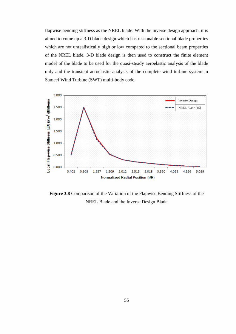
55

flapwise bending stiffness as the NREL blade. With the inverse design approach, it is

aimed to come up a 3-D blade design which has reasonable sectional blade properties

which are not unrealistically high or low compared to the sectional beam properties

of the NREL blade. 3-D blade design is then used to construct the finite element

model of the blade to be used for the quasi-steady aeroelastic analysis of the blade

only and the transient aeroelastic analysis of the complete wind turbine system in

Samcef Wind Turbine (SWT) multi-body code.

Figure 3.8 Comparison of the Variation of the Flapwise Bending Stiffness of the

NREL Blade and the Inverse Design Blade

Inverse Design

NREL Blade [15]

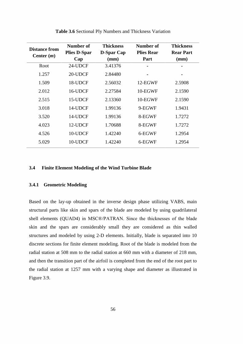
56

Table 3.6 Sectional Ply Numbers and Thickness Variation

Distance from

Center (m)

Number of

Plies D-Spar

Cap

Thickness

D-Spar Cap

(mm)

Number of

Plies Rear

Part

Thickness

Rear Part

(mm)

Root 24-UDCF 3.41376 - -

1.257 20-UDCF 2.84480 - -

1.509 18-UDCF 2.56032 12-EGWF 2.5908

2.012 16-UDCF 2.27584 10-EGWF 2.1590

2.515 15-UDCF 2.13360 10-EGWF 2.1590

3.018 14-UDCF 1.99136 9-EGWF 1.9431

3.520 14-UDCF 1.99136 8-EGWF 1.7272

4.023 12-UDCF 1.70688 8-EGWF 1.7272

4.526 10-UDCF 1.42240 6-EGWF 1.2954

5.029 10-UDCF 1.42240 6-EGWF 1.2954

3.4 Finite Element Modeling of the Wind Turbine Blade

3.4.1 Geometric Modeling

Based on the lay-up obtained in the inverse design phase utilizing VABS, main

structural parts like skin and spars of the blade are modeled by using quadrilateral

shell elements (QUAD4) in MSC®/PATRAN. Since the thicknesses of the blade

skin and the spars are considerably small they are considered as thin walled

structures and modeled by using 2-D elements. Initially, blade is separated into 10

discrete sections for finite element modeling. Root of the blade is modeled from the

radial station at 508 mm to the radial station at 660 mm with a diameter of 218 mm,

and then the transition part of the airfoil is completed from the end of the root part to

the radial station at 1257 mm with a varying shape and diameter as illustrated in

Figure 3.9.

57

Figure 3.9 Isometric View of the Skin Surfaces at the Root and the Transition Part of

the Blade

The remaining 8 sections are detailed by generating the front and the rear parts of the

blade sections, as shown in Figure 3.10. It should be noted that to facilitate the

assignment process of the material properties to the related blade sections, blade

sections are separated into 2 discrete parts.

Figure 3.10 Cross-Sectional View of the Finite Element Mesh of the Front and Rear

Part of the Skin of the Blade

58

Mostly, larger wind turbine blades have two spars, the front spar and the rear spar.

However, in the present study, original NREL blade design is followed. NREL blade

has only one spar to withstand the torsional and bending forces and it is located at

50% of the chord with no twist like the airfoil sections. Spar of the blade is modeled

by using the 2-D elements from the end of the transition part to tip of the blade with

a tapered thickness. Figure 3.11 shows the isometric view of the spar location of the

blade.

Figure 3.11 Isometric View of the Spar Location of the Blade

3.4.2 Mesh Generation and Property Assignment

After completing the geometrical model, each part of the blade section is finely

meshed by using Quad4 topology with the same global edge length in

MSC®/PATRAN. Then, all nodes are equivalenced with a tolerance of “0.005”to

eliminate duplicate nodes and create smooth links between the spar and the skin. In

the next step, surface normals of the pressure and suction side skins of the blade are

checked so as to verify that surface normals of the pressure and suction sides of the

blade skin all point inward assuming that female skin molds would be used in the

manufacturing of the skins of the blade. Figure 3.12 shows the finite element mesh of

different parts of the blade.

59

Figure 3.12 Finite Element Mesh of the NREL Blade

Totally, 20536 elements and 20427 nodes are used to generate the finite element

model. Element types and number of elements used in the geometric model are

detailed in Table 3.7.

Table 3.7 Number of Elements and Nodes Used in the Detailed Finite Element

Model of the Inverse Design Blade

Element Type: QUAD4

Shell Number of Elements Number of Nodes

Root 760 836

Transition 3640 3724

Skin 14591 14067

Spar 1535 1800

Total: 20536 20427

Before the property assignment, 2-D orthotropic materials E-Glass and Hybrid

Carbon/Fiberglass are defined. As shown in Figure 3.13, composite laminates that

are assigned to blade sections are created with an exact match of the orientation

angle of each ply as defined in the PreVABS input file.

60

Figure 3.13 Fiber Orientation and Material Assignment

As it was mentioned before, because of the lack of information about the complete

material layout used in the reference NREL blade, appropriate mass densities to the

materials in each blade section are assigned such that sectional mass densities of the

inverse design blade match the sectional blade mass densities of the NREL blade.

After subjective tuning and matching the desired sectional properties of the inverse

design blade with the NREL blade, total mass of the blade is calculated as 60.19 kg

where the original blade weighs 60.25 kg [15].

Table 3.8 Summary of Center of Gravity, Principal Inertias, Radii of Gyration, Mass

and Volume of the Inverse Design Blade

C.G (mm)

[x, y, z]

I-Principal

( )

Radii of Gyr.

(mm)

Mass

(kg)

Volume

( )

1.116E+002 8.279E+007 1.173E+003

2.390E+003 8.127E+007 1.162E+003 6.019E+001 1.140E+007

1.730E+001 1.830E+006 1.744E+002

61

Table 3.8 gives the summary of the center of gravity (CG), the principal inertias at

the CG, the radii of gyration corresponding to the principal inertias at the CG, mass

and volume of the inverse designed blade. To calculate the mass properties tabulated

above, shell thicknesses, cross-sectional areas concentrated mass values and densities

are used and the units are consistent with element properties, and material properties.

3.4.3 Application of the Boundary Conditions and Modal Analysis

The modal analysis of the inverse designed blade is performed by using solution

type, Normal Mode Analysis (Solution 103) in MSC®/NASTRAN. Before

conducting the analysis, all six degrees of freedom of the root nodes are fixed to

satisfy the required conditions as illustrated in detail in Figure 3.14. Before running

the modal analysis, weight conversion unit is set to 0.001 because geometric blade

modeling unit is done in millimeters.

Figure 3.14 Zoomed View of Fixed Root Nodes in MSC®/PATRAN

First and second flapwise bending mode shapes, first edgewise bending mode shape

and torsional mode shape are presented in Figure 3.15 - Figure 3.18. Global mode

shape results are also tabulated in Table 3.9. In order to make reliable comparison of

the quasi-steady aeroelastic analysis results that are obtained in MSC®/NASTRAN

with the results of the transient aeroelastic analysis of the wind turbine system that

62

are obtained in SWT, first few global mode shapes of the blade that is used in the

quasi-steady aeroelastic analysis should be matched with the first few global mode

shapes of the blade that is used in the transient multi-body dynamic analysis. It

should be noted that the multi-body dynamic model of the wind turbine which is

used in the transient aeroelastic analysis of the blade is presented in the next chapter.

Figure 3.15 1st Flapwise Bending Mode Shape of the Inverse Design Blade

[4.13 Hz]

Figure 3.16 1st Edgewise Bending Mode Shape of Inverse Design Blade

[8.13 Hz]

63

Figure 3.17 2nd

Flapwise Bending Mode Shape of the Inverse Design Blade

[14.69 Hz]

Figure 3.18 Torsional Mode Shape of the Inverse Design Blade

[24.52 Hz]

64

Table 3.9 Global Mode Shapes and Natural Frequency Results of the Inverse Design

Blade

Global Mode Shapes Natural Frequency Value [Hz]

1st Flapwise Bending 4.13 Hz

1st Edgewise Bending 8.13 Hz

2nd

Flapwise Bending 14.69 Hz

Torsional 24.52 Hz

3.5 Quasi-steady Aeroelastic Analysis

Quasi-steady aeroelastic analysis methodology is based on the coupling of an

aerodynamic model and structural finite element model. During the coupling

procedure, BEM based aerodynamic model provides the distributed loads over the

blade and structural model takes the distributed loads obtained from the aerodynamic

model as input and gravitational forces are superimposed on top of the aerodynamic

loads in order to analyze the blade deformation. The coupling of the aerodynamic

model and the structural finite element model progresses such that spanwisely

distributed loads create structural deformation which in turn causes an incremental

change in the aerodynamic loads. In the quasi-steady aeroelastic analysis, this

iterative process is repeated in a loosely coupled fashion until the blade deformation

converges to some value within a prescribed tolerance. The detailed algorithm of the

coupling procedure is introduced in Figure 3.19. In the loosely coupled approach,

BEM code is utilized to perform the aerodynamic analysis. In the BEM processing,

induction factors are estimated and according to known geometry, the inflow angles

and corresponding lift, drag, and thrust are calculated for each section.

65

Geometry

Modeling, Mesh

Generation and

Application of

Boundary

Conditions

BEM Analysis and Aerodynamic Load Calculation

Applying the

Aerodynamic

Loads over the 3-

D FE Model and

Superimposing

the Gravitational

and Centrifugal

Forces

Structural

Analysis and

Displacement

Calculation

Converged

YES

STOP

NO

Figure 3.19 Flow Chart of the Coupling Procedure [43]

66

Regarding the calculations, inductions factors are updated and iterative process

continues until a balanced response is reached within a prescribed tolerance. In the

next step, finite element model is coupled with the BEM results by applying the 2-D

aerodynamic lift, drag and moment on the aerodynamic center of the airfoil profile in

the structural model. Under the action of the aerodynamic loads, finite element

model deforms and hence, inflow angle and corresponding lift, drag, thrust and

torque for each section change incrementally. Incremental changes of the

aerodynamic forces, in turn, cause incremental changes in the structural deformation

of the blade. Therefore, this coupling process is repeated until convergence is

achieved based on a prescribed convergence criterion.

It should be noted that to perform the conventional algorithm for the BEM analysis

and aerodynamic calculation lift, drag and moment coefficients of the airfoil are

needed. Aerodynamic coefficients can be obtained from wind tunnel tests or

computational fluid dynamic (CFD) methods. In this study, for the NREL S809

airfoil, aerodynamic coefficients obtained from the wind tunnel tests conducted by

the Ohio State University (OSU) at Re=750.000 are used [41]. Figure 3.20 and

Figure 3.21 show the lift and the drag coefficient of the airfoil for varying different

Reynolds numbers.

Figure 3.20 Lift Force Coefficient Data of the NREL S809 Airfoil [41]

67

Figure 3.21 Drag Force Coefficient Data of NREL S809 Airfoil [41]

However, as it can be seen from the Figure 3.20 and Figure 3.21, the deep stall

effects are missing in wind tunnel test results. For this reason aerodynamic data at

high angle of attack are extrapolated by using NTWC design code “FoilCheck” [54]

which runs the Viterna-Corrigan equations for post stall process [41]. Figure 3.22 is

obtained after the airfoil data extrapolation from a limited range of angles to the

entire extended range and the results are used in the aerodynamic calculations. The

detailed aerodynamic lift, drag and moment coefficients are presented in APPENDIX

C.

68

Figure 3.22 NREL S809 Airfoil – Extrapolated Aerodynamic Force Coefficients

3.5.1 Results of Quasi-steady Aeroelastic Analysis for Concentrated Load

Cases

Initial aerodynamic loads are computed by following up the algorithm given in

Figure 3.19 for different wind conditions. However, only the results for the steady

wind speed 15 m/s with a wind shear exponent of 0.2 are presented in this study. To

verify that induction factors are within the prescribed tolerance, 30 iterations have

been performed for each blade element and to speed up the induction factor

estimation process, a wind turbine performance predictor tool, WT_Perf [53] which

is developed by National Wind Technology Center (NTWC) is used. The program is

written in FORTRAN 95 language, and it is designed to perform measurements for

angle of attack values ranging from 0 degrees to ±180 degrees. Azimuthal

representation of the wind turbine blades are illustrated in Figure 3.23.

69

Figure 3.23 Azimuth Positions of the NREL Blade

To run the BEM analysis in WT_Perf, an input file which includes wind turbine

model configuration, algorithm configuration, turbine data and geometrical data of

NREL blade is prepared as shown in APPENDIX B - Part A in detail. Moreover,

Prandtl’s tip-loss, hub-loss models and swirl effects are enabled in the input file and

these input files are coupled with the 2-D airfoil aerodynamic data by utilizing the

WT_Perf program and some of the results obtained by WT_Perf are shown in Figure

3.24 and Figure 3.25 .

70

Figure 3.24 Axial and Tangential Induction Factor Variations of NREL S809

Figure 3.24 shows the extracted axial and tangential induction factors. As it can be

seen that tangential induction factor decreases gradually and at the tip it is equal to 0

which is an expected result because of the Prandtl’s tip loss correction.

In the next step, induction factors determined, inflow velocities, angle of attacks and

aerodynamic coefficients at each section are used to compute the lift, drag and

moment forces (Eqn. (2.14) – Eqn. (2.16)). Figure 3.25 shows the in-flow angle and

angle of attack variations of the NREL S809 blade calculated by WT_Perf. Finally,

by applying Eqn. (2.24) and Eqn. (2.25) tangential and normal forces are calculated

for 20 sections, as shown in Figure 3.26.

0 2 4 6 8 10 12 14 16 18 200

0.05

0.1

0.15

0.2

0.25

0.3

0.35

0.4

0.45

0.5

Induction Factor Variations at Wind Speed of 15[m/s]

Section Numbers

ND

Axia

l and T

angentia

l Inductio

n F

acto

rs

Axial Induction Factor

Tangential Induction Factor

71

Figure 3.25 In-flow Angle and Angle of Attack Variations of the NREL S809 Blade

- Azimuth 0

Figure 3.26 Normal and Tangential Force Variations of NREL S809 Airfoil –

Azimuth 0

0 2 4 6 8 10 12 14 16 18 200

10

20

30

40

50

60

70

80

In-flow and Angle of Attack Variations at Wind Speed of 15 [m/s]

Section Numbers

Degre

e

In-Flow Angle

Angle of Attack

0 2 4 6 8 10 12 14 16 180

10

20

30

40

50

60

70

80

90

100

110

Normal and Tangential Force Variations at Wind Speed of 15[m/s]

Section Numbers

Norm

al a

nd T

angentia

l Forc

e (

N)

Normal Force

Tangential Force

72

To distribute the calculated normal, tangential force and moment forces over the

blade, 20 nodes are defined at %25 chord of the blade measured from the leading

edge of the blade and circular root sections. Then, the forces normal and tangential to

the global coordinate lines and moments are placed on the defined nodes at the upper

layer of the blade as shown in Figure 3.27.

Figure 3.27 Location of Aerodynamic Force Application Nodes and Loads Applied

to the Inverse Design Blade for Flapwise Deflection Calculation

After all the loads are applied over the finite element model of the NREL blade,

static analysis is conducted by using the solution sequence 101 of

MSC®/NASTRAN to calculate the flapwise deflection at the tip of the blade. As a

result of static analysis, displacement at the tip of the blade is obtained as 114.35 mm

for the 1st Iteration as shown in Figure 3.28.

Normal Force = 45.12 N

Tangential Force = 7.429 N

Moment = 8.780 N*m

73

Figure 3.28 Blade Deflection at 72 rpm and 15m/s Wind Speed – After the 1st

Iteration

After the 1st deformation, inflow angle and corresponding aerodynamic loads and

moments are re-calculated for each section. Incremental changes in the aerodynamic

loads are computed by utilizing the “shifting nodes” feature of MSC®/PATRAN. As

illustrated in Figure 3.29, all node locations are shifted to the deformed positions.

After the shifting of the nodes, new positions of the node locations at the leading and

trailing edges are recorded. These recorded locations are compared with the non-

deformed node location data and by using the simple trigonometric formulas,

differences in the inflow angle and twist angle are computed. Inflow angle and twist

values are added to the initial ones and all the aerodynamic loads are re-computed

utilizing the newly calculated inflow angle and twist values by performing BEM

analysis at WT_Perf tool. This coupling process is repeated until convergence is

achieved based on a prescribed convergence criterion which is decided as the 0.01

mm for the difference of tip deflection results between the iterations. Figure 3.30 and

Figure 3.31 show the 2nd

and 3rd

displacement field of the wind turbine blade for

Azimuth 0 – Vertical up position of the blade.

74

Figure 3.29 Deformed Blade and Shifted Node Locations

Figure 3.30 Blade Deflection at 72 rpm and 15m/s Wind Speed – After the 2nd

Iteration

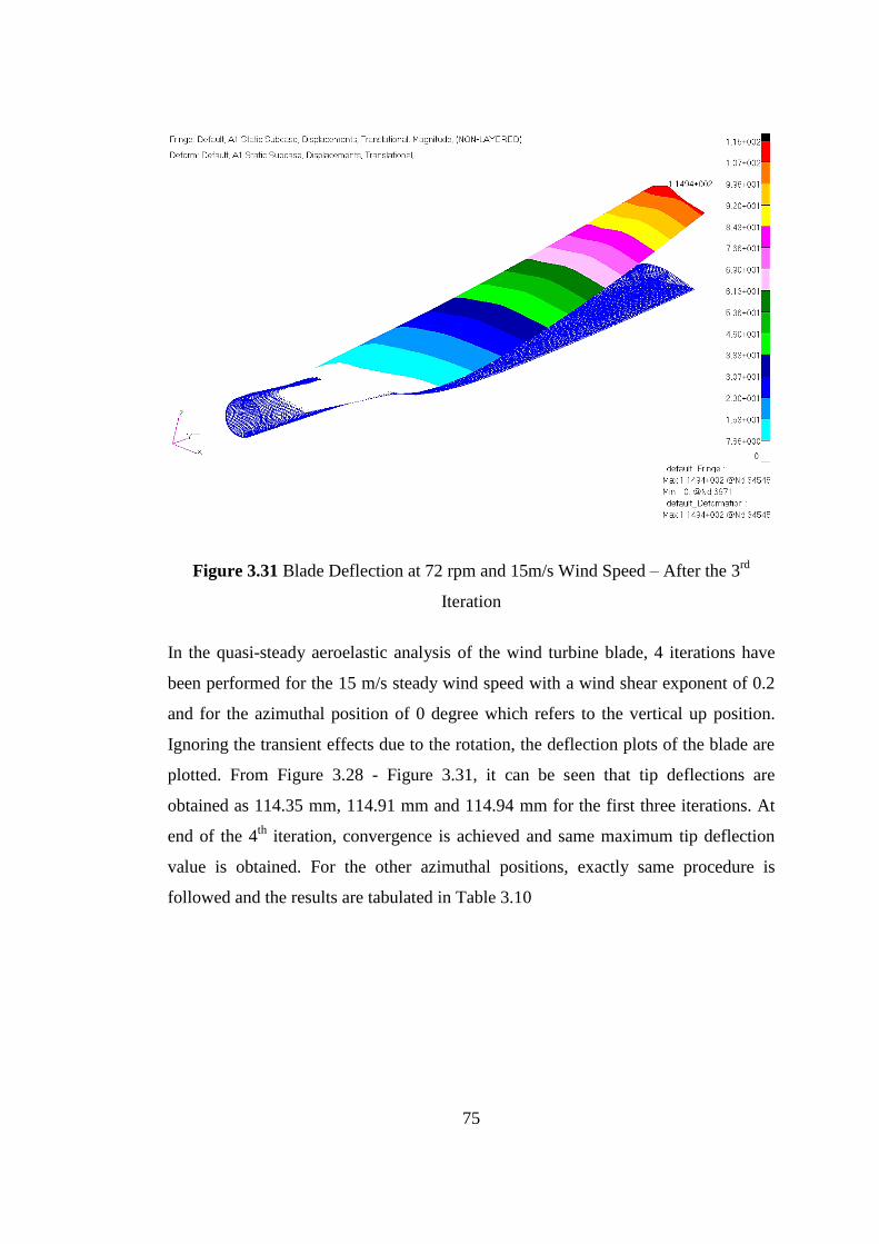
75

Figure 3.31 Blade Deflection at 72 rpm and 15m/s Wind Speed – After the 3rd

Iteration

In the quasi-steady aeroelastic analysis of the wind turbine blade, 4 iterations have

been performed for the 15 m/s steady wind speed with a wind shear exponent of 0.2

and for the azimuthal position of 0 degree which refers to the vertical up position.

Ignoring the transient effects due to the rotation, the deflection plots of the blade are

plotted. From Figure 3.28 - Figure 3.31, it can be seen that tip deflections are

obtained as 114.35 mm, 114.91 mm and 114.94 mm for the first three iterations. At

end of the 4th

iteration, convergence is achieved and same maximum tip deflection

value is obtained. For the other azimuthal positions, exactly same procedure is

followed and the results are tabulated in Table 3.10

76

Table 3.10 Results of Quasi-steady Aeroelastic Analysis for Concentrated Loads

# of

Iterations

Tip

Displacement

Azimuth 0

(mm)

Tip

Displacement

Azimuth 90

(mm)

Tip

Displacement

Azimuth 180

(mm)

Tip

Displacement

Azimuth 270

(mm)

1st Iteration 114.35 109.60 104.38 109.60

2nd

Iteration 114.91 110.61 105.04 110.61

3rd

Iteration 114.94 110.69 105.15 110.69

4th

Iteration 114.94 110.69 105.15 110.69

3.5.2 Results of Quasi-steady Aeroelastic Analysis for Distributed Load Cases

In the second part of the quasi-steady aeroelastic analysis, similar procedure has been

followed to calculate the aerodynamic loads. As a difference from the initial study,

turbine model is divided into 10 discrete sections in WT_Perf as detailed in

APPENDIX - Part B to achieve a close match with the aerodynamic model of the

transient aeroelastic analysis. After obtaining the induction factors normal, tangential

forces and aerodynamic moments are calculated and applied on a node at the center

of the each section and at the %25 chord line of the airfoil.

Concentrated aerodynamic forces acting at the aerodynamic center of blade sections

are distributed to the suction side nodes of the finite element model by means of

multi-point constraint element RBE3 that is available in MSC®/NASTRAN. RBE3

element defines a constraint relation in which the motion at a reference grid point is

the least square weighted average of the motions at other grid points. Forces and

moments applied to reference points are distributed to a set of independent degrees of

freedom based on the RBE3 geometry and local weight factors. The manner in which

the forces are distributed is analogous to the classical bolt pattern analysis. The force

and moment is transferred directly to the weighted center of gravity location along

with the moment produced by the force offset. The force is distributed to the bolts

77

proportional to the weighting factors. The moment is distributed as forces, which are

proportional to their distance from the center of gravity times their weighting factors.

For the distribution of the forces applied at the aerodynamic center, weight factors

are taken as 1 since nodes represent same size bolts. For this purpose, the nodes

created at the aerodynamic center of the blade sections are defined as the dependent

node and all six degrees of freedom are defined. The nodes in the suction side of the

blade sections are selected as the independent nodes and just translational degrees of

freedom are selected. Figure 3.32 shows the distribution of aerodynamic forces

applied at the aerodynamic center to suction side nodes by RBE3 elements.

Figure 3.32 RBE3 Elements and Distribution of the Aerodynamic Loads Applied at

the Aerodynamic Center to Upper Section Nodes

Once the coupling between finite element model and aerodynamic forces which are

calculated by WT_Perf at the aerodynamic center of each blade is completed, static

78

analysis is conducted as described previously. For azimuth 0 degree, after the 1st

iteration, the maximum displacement is obtained as 111.06 mm at the tip of the blade

as shown in Figure 3.33.

Figure 3.33 Flapwise Deflection at 72 rpm and 15m/s Wind Speed – After the 1st

Iteration

Again by following the same procedure as detailed in the concentrated load case,

after the 1st deformation, incremental changes in angle of attack values are computed

for each azimuth location and corresponding aerodynamic loads and moments are re-

calculated for each blade section. As an example, for azimuth 90 degrees, Table 3.11

gives the incremental changes in angle of attack values with the iteration number at

each blade element. The first blade element corresponds to the circular root where

there is no lift. From Table 3.11, it is seen that in three iterations incremental changes

in the angle of attack values become almost negligible. The fourth iteration

essentially gives the same deformation of the blade as the third iteration.

79

Table 3.11 Incremental Changes in Angle of Attack Values with the Iteration

Numbers (Azimuthal Position - 90 Degree)

Blade Element 1st iteration (Deg.) 2

nd iteration (Deg.) 3

rd iteration (Deg.)

2 -0.0222 -0.0150 -0.00003

3 -0.2715 -0.0129 -0.00021

4 -0.3396 -0.0068 -0.00025

5 -0.4030 -0.0086 -0.00030

6 -0.4219 -0.0011 -0.00031

7 -0.4374 0.0038 -0.00031

8 -0.4290 0.0052 -0.00031

9 -0.4628 0.0046 -0.00034

10 -0.4384 0.0065 -0.00029

Table 3.12 gives the maximum tip displacements obtained as a result of quasi-

aeroelastic analysis at three different azimuthal locations.

Table 3.12 Results of Quasi-steady Aeroelastic Analysis for Distributed Loads

# of

Iterations

Tip

Displacement

Azimuth 0

(mm)

Tip

Displacement

Azimuth 90

(mm)

Tip

Displacement

Azimuth 180

(mm)

Tip

Displacement

Azimuth 270

(mm)

1st Iteration 111,06 102,82 99,95 102,82

2nd

Iteration 112,14 103,52 100,14 103,52

3rd

Iteration 112,22 103,61 100,38 103,61

4th

Iteration 112,22 103,61 100,38 103,61

From the results presented in Table 3.10 and Table 3.12, it is seen that the change in

the maximum tip displacement is very small in each iteration. This is an indication

that the inverse design blade structure is actually very rigid. However, the whole

process of quasi-steady aeroelastic analysis would not change if the blade structure

was more flexible. It should be noted that present analysis only deals with linear

structures. Material and geometric non-linearity is not considered. In general,

material non-linearity is not a concern in wind turbine blades. But, geometric non-

linearity associated with the large deflections and rotations can be important for long

80

and flexible blade structures. For very flexible blade structure, quasi-steady

aeroelastic analysis could still be performed if geometrically non-linear solver

MSC®/NASTRAN (Sol 106) is used as the structural solver instead of linear solver

Sol 101. It is also noted that for the distributed load case, maximum tip

displacements are less than the maximum tip displacements obtained by the

concentrated load case.

In Chapter 4, comparisons are made with the deflection results of the transient

aeroelastic analysis of the wind turbine system which is performed in Samcef Wind

Turbine.

81

CHAPTER 4

MULTI-BODY MODELING of the REFERENCE TURBINE AND

TRANSIENT AEROELASTIC ANALYSIS OF THE BLADE

In the design of wind turbine blades, for accurate load analysis, complete turbine

model has to be built in a multi-body framework and transient aeroelastic analysis of

the wind turbine system which includes major components such as turbine blades,

rotor hub and rotor shaft, gearbox, generator and tower has to be performed. Building

the multi-body model of the complete wind turbine requires specialized software and

detailed information about the major components which build-up the turbine system.

For this purpose, a multi-body dynamic code “Samcef Wind Turbine (SWT)” [55] is

utilized for performing the transient aeroelastic analysis of the blade. “Samcef Wind

Turbine” integrates the aerodynamic, structural and control features of the wind

turbine in a fully dynamic environment. Aerodynamic solver of SWT is based on

BEM theory with typical corrections such as tip and hub losses, tower shadow, and

deactivation of induction factors at low tip speed ratios. SWT also has built-in semi-

empirical sub-models to treat unsteady aerodynamics with higher accuracy.

Specifically, SWT has dynamic wake sub-model, skewed flow correction sub-model

and dynamic stall sub-models which are of Beddoes-Leishman type. The controller is

integrated to the wind turbine model by means of dynamic link library which can be

used for typical wind turbine simulations. Multi-body simulation of the wind turbine

system is performed by the implicit non-linear finite element solver Samcef Mecano

[56] which has the ability to allow the use of multi-body simulation features, such as

kinematic joints etc., inside real finite elements models. Transient simulations are

performed in time domain taking into account the structural, multi-body,

aerodynamic and control features in a fully non-linear dynamic way with strong

82

coupling. The main non-linear features are present in the aerodynamics, in the

controller, and in structural and multi-body elements such as non-linear stiffness,

large rotations, bearing gaps etc. [55].

In the present study, to conduct the multi-body dynamic analysis of the wind turbine

system, firstly, dynamic superelement of the turbine blade has to be created in the

Samcef Field [16] environment since Samcef Wind Turbine recognizes the format of

the superelement generated by Samcef Field. Dynamic superelement of the blade is

then introduced into the multi-body model of the wind turbine system, and transient

aeroelastic analysis is performed in steady wind conditions. Before the generation of

the dynamic superelement of the blade, three dimensional finite element model of the

blade is created in Samcef Field in a similar manner to the creation of the finite

element model in MSC®/PATRAN that is described before. It should be noted that

in order to reflect the stiffness and mass properties of the blade, that is generated in

two different finite element programs MSC®/NASTRAN-PATRAN and Samcef

Field, accurately, three dimensional finite element model of the blade is used rather

than the beam model. Another reason for the choice of the three dimensional finite

element model of the blade is that neither MSC®/NASTRAN nor SWT have beam

formulation that is suitable for modeling composite blades with coupling

coefficients. On the other hand, three dimensional finite element models are too

costly to be used in the multi-body simulation of the complete wind turbine system.

Therefore, in SWT superelement of the blade is used for the multi-body simulation

of the wind turbine system.

4.1 Generation of Superelement Blade

In the present study, transient aeroelastic response of the turbine blade is investigated

by the multi-body simulation of the reference wind turbine system. Superelement of

the wind turbine blade, which is completed through the inverse design process

described previously, is created in Samcef Field [16] and introduced into the multi-

83

body model of the wind turbine system which is generated in Samcef Wind Turbine

Dynamic superelement used in the present study is non-linear superelement which is

based on the Craig and Bampton component mode method [57]. Non-linearities arise

from the fact that formulation of the superelement allows modeling of the blade

structure undergoing large displacements and rotations in space, with the only

limitation that with respect to the local frame fixed to the blade, blade behaves

geometrically linear. The main advantage of using the dynamic superelement of the

blade in the multi-body dynamic model of the wind turbine system is to allow the

detailed modeling of components with complex geometry and structural function

while keeping a relatively simple global dynamic model with the smallest number of

degrees of freedom possible [47]. It should be noted that since dynamic superelement

is created from three dimensional finite element models of the blade, superelement

possesses the whole coupling effects.

For creating the superelement model of the blade, initially, CAD drawing of the

NREL Blade is exported in a “Step” format from MSC®/PATRAN and then the file

is imported to the Samcef Field. Before the import process, the coordinates of the

blade are modified to meet the specifications of the Samcef Field tool. As indicated

in Figure 4.1, rotor blade span axis is defined along the z axis while the chord length

is varied along the y axis. Furthermore, blade root is moved from 0.508 m to central

coordinate point (0, 0, 0).

84

Figure 4.1 Isometric View of the Blade Geometry in Samcef Field

In the next step, physical and mechanical properties of the E-Glass and Prepreg the

Hybrid Carbon/Fiberglass composite are defined and assigned to the related 10 cross-

sections with varying lay-up numbers and orientations. It should be noted that, the

same mass tuning that has been applied in finite element model that is created in

MSC®/PATRAN, is also repeated in Samcef Field too. After generating the shell

model of the blade in graphical user interface, retained nodes are created. For the

superelement generation, for each selected cross-section, for the airfoil sections, a

retained node must be created at the %25 chord of the blade measured from the

leading edge of the blade. At the root section of the blade since the geometry is

circular, retained node is placed at the center of the circular cross-section. Once the

superelement of the blade is imported into the multi-body model of the wind turbine

system, retained nodes are used for applying external loads on the turbine blade.

Retained nodes are also used as the connector nodes of the blade to the wind turbine

system through the rotor hub. Therefore, at the root section retained node is created

at the center of the circular cross-section. This node is also used as the pitch axis

location through which the controller in the multi-body model of the wind turbine

system controls the rotation of the blade about the pitch axis. Figure 4.2 shows the

85

retained nodes those are placed at the center of the each section and at the %25 chord

of the airfoil sections of the blade measured from the leading edge of the blade.

Figure 4.2 Generation of the Retained Nodes and Mean Elements

To complete the superelement model, each retained node should be connected to the

face of the corresponding section of the blade as shown in Figure 4.2. In this study,

connection of the retained node with the sections of the blade is established by using

the mean element that is defined in Samcef Field. Mean elements connect the

retained node, which is taken as the slave node, to the master nodes on the faces of

the particular section. By the use of mean elements, mean displacement of the master

nodes is assigned to the retained node. Thus, retained node reflects the deformation

of the blade section to which it is connected. It should be noted that in the generation

of the superelement of the wind turbine blade correct displacement boundary

condition must be assigned to the retained node at the root of the blade which

connects the blade to the rotor hub in the wind turbine system. At this connection

node, a free rotation about pitch axis must be defined to allow for the pitch motion of

the blade in the multi-body simulation of the wind turbine system. In the final step of

86

superelement generation, finite element mesh of the blade structure is created. Fine

finite element mesh with a length of 0.03 m is generated on the whole blade

structure. The reason for selecting the specified mesh length is to have close element

and degree of freedom numbers with the finite element model generated in

MSC®/PATRAN and used in quasi-steady aeroelastic analysis. . During the mesh

generation process, finite element nodes are also created on retained nodes and the

dynamic superelement of the blade is generated based on the Craig and Bampton

component mode method.

In the superelement blade model, the retained node that is at the root of the blade is

fixed. In the three dimensional model the root section of the blade that is connected

to the retained node is fixed. Figure 4.3 shows the isometric view of the meshed

blade. The root section of the blade is zoomed to show the clamped root closely.

Figure 4.3 Isometric View of the Meshed Blade

To verify the superelement of the blade, modal analyses are performed for the three

dimensional blade and for the superelement blade which are both clamped at the

root. Free vibration frequencies for the 1st and 2

nd flapwise bending, 1

st edgewise

87

bending and 1st torsional vibration modes, which are obtained for the 3-D finite

element model of the blade, are compared with the natural frequencies of the

superelement of the blade and natural frequencies obtained by the modal analysis of

the 3-D finite element model in MSC®/NASTRAN. Natural frequency results are

compared in Table 4.1. As it is seen from the 2nd

and 3rd

column of Table 4.1, there

exists a good agreement between the natural frequencies obtained by the 3-D FE

model generated in Samcef Field and the natural frequencies obtained by the

superelement of the blade. Good agreement is an indication that the superelement

model represents the mass and stiffness properties of the 3-D blade structure

accurately. In the 4th

column of the table the natural frequencies of the finite element

model generated in MSC®/NASTRAN are shown. It is seen that there exist slight

differences between the natural frequencies of the 3-D Samcef FE model and the 3-D

MSC®/NASTRAN FE model. The reason for differences in the natural frequencies

of some modes could be due to the different solvers of Samcef and

MSC®/NASTRAN. However, these differences are considered to be in an acceptable

tolerance range and do not significantly affect the comparison results of quasi-steady

and transient aeroelastic analysis. Figure 4.4 - Figure 4.7 show the modes shapes of

the superelement blade corresponding to the lowest natural frequencies

Table 4.1 Comparison of the Natural Frequencies

Global Mode

Shapes

3-D FE Model

in Samcef Field

(Hz)

Superelement

Model Samcef

Field (Hz)

3-D FE Model in

MSC®/NASTRAN

(Hz)

1st Flapwise Bending 4.13 4.13 4.13

1st Edgewise Bending 8.32 8.33 8.13

2nd

Flapwise Bending 17.52 17.54 14.69

Torsional 28.40 28.44 24.52

88

Figure 4.4 1st Flapwise Bending Mode Shape of the Superelement Blade Model

[4.13 Hz]

Figure 4.5 1st Edgewise Bending Mode Shape of the Superelement Blade Model

[8.32 Hz]

89

Figure 4.6 2nd Flapwise Bending Mode Shape of the Superelement Blade Model

[17.52 Hz]

Figure 4.7 Torsional Mode Shape of the Superelement Blade Model [28.40 Hz]

4.2 Wind Turbine Modeling in Samcef Wind Turbine

To study the aeroelastic response of the superelement blade, a 20 kW multi-body

wind turbine model is created in Samcef Wind Turbine. For realistic and reliable

90

computation of the internal loads in the wind turbine system, several sub-structures,

including the controller, must be included in the multi-body model of the turbine. For

the parameters of the wind turbine, known properties of NREL’s turbine is taken as

the reference [15]. For the drive train model, the so-called FAST drive train model

that is available in the Samcef Wind Turbine is included in the wind turbine multi-

body dynamic model. FAST drive train includes the bedplate, simple gearbox and

generator, rotor shaft, coupling shaft, nacelle, main frame and rear frame. When

FAST drive train is used, it is not necessary to include components of the drive train

separately into the multi-body model of the wind turbine system. In case of separate

inclusion of the drive train components, detailed properties must be provided for

each component. Therefore, in the present study, to keep the modeling effort of the

wind turbine system simple, FAST drive train is used. Figure 4.8 and Table 4.2 -

Table 4.4 show the wind turbine and properties of the components used in the multi-

body simulation of the wind turbine system.

Figure 4.8 Multi-body Model of the Wind Turbine Parts [55]

91

In order to include only the transient effects due to the rotation of the wind turbine

blades in the multi-body simulation of the wind turbine system, multi-body model of

the wind turbine is created with almost rigid drive train and tower as the main sub-

structures. By assigning a modulus of elasticity of 1000 times the modulus of

elasticity of steel to the tower, flexibility of the tower is eliminated. Similarly,

equivalent drive shaft torsional spring constant value is also increased 1000 times

compared to the default value given for the Fast drive train in SWT. By eliminating

the flexibility of the drive train and the tower, more realistic comparison of the

results of the transient aeroelastic analysis of the complete wind turbine system with

the results of the quasi-steady aeroelastic analysis of the turbine blade can be made.

Table 4.2 Tower Properties Used in the Multi-body Simulation of the Wind Turbine

System

Tower Properties

Tower Height 11.5 m

Upper External Diameter 0.4064 m

Upper Internal Diameter 0.3636 m

Lower External Diameter 0.6096 m

Lower Internal Diameter 0.5746 m

Tower Material Young Modulus 210 E+12 Pa

Tower Material Poisson Ratio 0

Tower Material Density 7.8 E+03 kg/

Tower Height 11.5 m

Upper External Diameter 0.4064 m

92

Table 4.3 Blade Properties Used in the Multi-body Simulation of the Wind Turbine

System

Blade Properties

Blade Model Type Super Element

Number of Blades 3

Blade Length 4.521 m

Rotor Conicity/Tilt Angle 0/0

Hub Diameter 1.016 m

Hub Total Mass 237.8 kg

Hub Inertia about Shaft Axis 118 kg.

Link Between Hub and Blades Rigid

Table 4.4 Samtech Controller & Fast Drive Train Properties in the Multi-body

Simulation of the Wind Turbine System

Samtech Controller & Fast Drive Train Properties

Constant Generator Torque 2.6 E+03 N.m

Constant Pitch Angle 0

Angular Speed Constant 72 R.P.M

Nacelle Total Mass 1.712 E+03 kg

Nacelle Inertia about Yaw Axis 3.789 E+03 kg*

Gearbox Ratio 25.13

Equivalent Drive Shaft Torsional Spring Constant 3.48 E+06 kg. / .deg

Generator Inertia about High-speed Shaft 0.22644 kg.

Max Torque Delivered by the Disk Brake System 115 N.m

While creating the complete wind turbine system model by defining the structural

properties of the simple tower, superelement blades, Samtech controller and Fast

drive train, the global coordinates are defined as shown in Figure 4.9. In the wind

turbine model defined in SWT, x axis is parallel to the rotor axis, z axis is the vertical

93

axis perpendicular to the rotor, and y axis is perpendicular to both x and z axes. The

global coordinate frame is defined as a fixed frame which does not rotate.

Figure 4.9 Multi-body Dynamic Model of the Wind Turbine System

For the aeroelastic simulations, the calculation of aerodynamic loads is one of the

main aspects for the computational tool considered. For this purpose, 2-D

aerodynamic data obtained from wind tunnel experiments are introduced to the rotor

system to capture the external loads and tip deflection results accurately.

Aerodynamic coefficients of the circular cross-section are assigned to root part and

then for the airfoil sections aerodynamic coefficients of the NREL S809 airfoil are

assigned to the remaining sections of the superelement blade as shown in Figure

4.10. The aerodynamic lift, drag and moment coefficients are presented in

APPENDIX C.

Figure 4.10 Assignment of the Aerodynamic Coefficients to Multi-body Dynamic

Model of the Wind Turbine System

94

It should be noted that the main interest in the transient aeroelastic analysis is to

obtain the structural loads and the tip deflections of the blade accurately hence, there

is no need to focus on the generated power. For this purpose, a constant function is

defined in time domain and the angular speed of the rotor is set to constant angular

speed of 72 rpm as illustrated in Table 4.5. Then, the created constant function is

assigned to control node as shown in Figure 4.11. This control node assures that the

low speed shaft of the wind turbine rotates at constant 72 rpm.

Table 4.5 Constant Function Table Defined in Multi-body Dynamic Model of the

Wind Turbine System

Function Name X-axis Units Y-axis Units Value

ConstantFunc_72rpm Time Angular Speed 72 rpm

Figure 4.11 Assignment of the Constant Function to Control Node

For the transient analysis, the aerodynamic conditions such as the direction and the

speed of the wind are set as constant upwind at 15 m/s for the load case. For the

advanced aerodynamic options, except for the tip losses which are also taken into

account in the WT_Perf calculations, as it is seen from Figure 4.12, no other

unsteady effects are considered in the transient analysis. These procedures are

detailed in APPENDIX D.

95

Figure 4.12 Advanced Aero Options for Transient Analysis

As far as the controller is concerned, both the pitch angle and the rotor speed are

imposed, thus the controller does not have any effect on the simulation.

Table 4.6 Rated Load Case Defined in Multi-body Dynamic Model of the Wind

Turbine System

Name Wind Speed Rotor Speed Blade Pitch

Rated Load Case 15 m/s 72 rpm 0 deg.

After the load case and the constant function angular velocity are created, one

transient analysis is generated with duration of 30 seconds. In the results part, it can

be seen that all the results quickly converge to their steady state value and this points

that the transient aeroelastic analysis of the superelement blade has been completed

without failure.

4.3 Results of the Transient Aeroelastic Analysis

According to chosen sensors, SWT gives plenty of results but in this study only the

few required sensor results are presented. Figure 4.13 shows the total force acting

normal to the global coordinate system calculated by the Samcef BEM code over the

superelement blade. As it is seen from, obtained normal forces for the azimuth 0 are

higher than rest which is an expected result. Due to the wind shear exponent, wind

96

speed increases with an increasing height and this creates an increase in the amount

of normal force over the sections of the blade. In Figure 4.13, the numbers on the

plot show correspond to the normal force values for the 0 degree azimuthal position.

Figure 4.13 Normal Force Variation across the Blade for Different Azimuthal

Positions

Figure 4.14 and Figure 4.15 show the tangential force and moment variations across

the blade. The tangential force and moment increase gradually with the radial

distance, and because of the non-uniform circulations at the tip, generated moment

and force decrease towards the tip section.

97

Figure 4.14 Tangential Force Variation across the Blade for Different Azimuthal

Positions

Figure 4.15 Moment Variation across the Blade for Different Azimuthal Positions

Figure 4.16 and Figure 4.17 give the axial and tangential tip displacement of the

superelement blades respectively. The maximum tip displacement converges to a

value of almost 116.50 mm and the lowest tip displacement is obtained as 98.15 mm.

In this case, it should be explained that that maximum tip displacement does not

98

correspond to 0 degree azimuthal position but it is observed at the azimuthal position

of 45 degree.

Figure 4.16 Axial Tip Displacement of the Blade towards Downwind

Figure 4.17 Tangential Tip Displacement of the Blade towards Next Blade

99

In Table 4.7, sectional axial and tangential tip displacements are detailed for different

azimuthal positions. From Table 4.7, it can be seen that tip deflection for the azimuth

0 is obtained as 114.368 mm which is quite close the tip deflection value obtained

from the quasi-steady aeroelastic analyses.

For the other azimuthal positions, comparison of the blade tip deflections obtained by

the transient analysis of the complete wind turbine system with the blade tip

deflections obtained by the both quasi-steady aeroelastic analyses is done in Table

4.8. In the last column of the table, ratios of the tip deflections are presented. Table

4.8 clearly shows that because of the wind shear effect, tip deflection at the 0 degree

azimuthal position, which corresponds to the vertically up position of the blade, is

higher than the tip deflections at the other azimuthal positions. It is also noted that tip

deflections determined by the quasi-steady aeroelastic analysis with concentrated

loads are higher than the tip deflections determined by the transient analysis of the

wind turbine system. However, ratio column of Table 4.8 shows that tip deflections

determined by the quasi-steady aeroelastic analyses are within %10 of the tip

deflections determined by the transient analyses for different azimuthal positions.

Moreover, it is seen that tip deflection results of quasi-steady aeroelastic analyses

with the distributed load case are closer to the tip deflection results obtained by the

transient aeroelastic analysis a than the tip deflection results obtained by the

concentrated load case.

It can be considered that if the same finite element solver is used for quasi-steady

aeroelastic analysis and superelement blade generation, then the differences in the tip

deflections would be lower. It should be noted that in the present study,

MSC®/NASTRAN is chosen as the finite element solver to make use of the “shifting

nodes” feature of MSC®/PATRAN so that aerodynamic loads can be applied on the

deformed configuration of the blade. It is considered that quasi-steady aeroelastic

analyses can be used reliably in the preliminary design stage to perform design

iterations to come up with a blade structure that satisfies a certain stiffness

100

requirement. Obviously, in the detailed design phase, multi-body simulations of the

wind turbine system have to be performed for detailed analyses.

Table 4.7 Axial and Tangential Tip Displacement Variations at Different Azimuthal

Positions

# of

Section

AxialDisp

Azimuth

0 (m)

TangDisp

Azimuth

0 (m)

AxialDisp

Azimuth

90 (m)

TangDisp

Azimuth

90 (m)

AxialDisp

Azimuth

180 (m)

TangDisp

Azimuth

180 (m)

1 2.33E-12 1.16E-09 2.22E-12 4.93E-09 2.10E-12 1.03E-09

2 0.001444 0.000273 0.001326 1.28E-06 0.001234 0.000322

3 0.005043 0.001092 0.004491 0.00032 0.004329 0.001147

4 0.011759 0.002897 0.010377 0.001457 0.010159 0.002825

5 0.023475 0.005634 0.020803 0.003252 0.020377 0.005354

6 0.037656 0.008668 0.033564 0.005293 0.032763 0.008157

7 0.052568 0.011715 0.046983 0.007333 0.045767 0.010971

8 0.069116 0.014796 0.061929 0.009389 0.060184 0.013816

9 0.086777 0.017802 0.077908 0.011362 0.075556 0.016593

10 0.114368 0.022331 0.102899 0.014343 0.099554 0.020785

Table 4.8 Comparison of the Tip Deflection Results

Azimuth

Positions

(degree)

Tip Displacement

(Quasi-steady)

Concentrated

Load Case (mm)

Tip Displacement

(Quasi-steady)

Distributed Load

Case (mm)

Tip Displacement

(Transient)

(mm)

Ratios

0 114.94 112.22 114.368 1.005/0.981

90 110.69 103.61 102.899 1.076/1.007

180 105.15 100.38 99.554 1.056/1.008

270 110.69 103.61 102.899 1.076/1.007

One last comparison is performed between the flapwise bending moment of quasi-

steady aeroelastic analyses and the flapwise bending moment of the transient

101

aeroelastic analysis. In Table 4.9, the comparison of the flapwise bending moments

at the end of the cylindrical region (r=0.66 m) for different azimuthal positions are

presented. The bending moments are calculated by utilizing the results of blade

element momentum calculations performed in WT_Perf and SAMCEF. Once the

sectional forces are calculated, root bending moment is calculated by summing the

moment contribution of each sectional force.

Table 4.9 Flapwise Bending Moments at r=0.66 m Calculated for the Constant Wind

Speed (15 m/s).

Azimuth

Positions

Flapwise Moment

Concentrated Load

Case with 20 Blade

Sections (N.m)

Flapwise Moment

Distributed Load

Case with 10 Blade

Sections (N.m)

Flapwise Moment

Transient

(N.m)

0 3711,121 3612.281 3687.545

90 3559,388 3480.198 3495.479

180 3328,284 3262.835 3255.559

From Table 4.9, it is seen that the flapwise bending moments calculated utilizing the

output of WT_Perf for the concentrated loads case of quasi-steady aeroelastic

analysis are higher than the flapwise root bending moments calculated by SWT. The

reason for the difference is due to the fact that in WT_Perf, for the concentrated load

case 20 blade segments are used in the analysis whereas in SWT 10 blade segments

are used. For the distributed load case same numbers of segments (10 segments) are

used in both WT_Perf and in SWT. Therefore, for distributed load case with the

same number blade segments as the transient aeroelastic analysis, similar force

distribution is obtained, and better approximation of the root bending moment is

achieved. It should also be noted that the reason for the difference in the tip

displacements obtained by the quasi-steady aeroelastic analysis with the concentrated

102

load case and the transient analysis can be mainly attributed to the higher loads used

in the quasi-steady aeroelastic analysis.

103

CHAPTER 5

CONCLUSION

This thesis aims to present a comparison study of quasi-steady and transient

aeroelastic analysis of a composite wind turbine blade in steady wind conditions. To

conduct quasi-steady aeroelastic analysis, inverse design methodology is applied to

build up a reference turbine blade to be used in the aeroelastic analysis. Blade of the

unsteady aerodynamics experiment (UAE) research wind turbine is taken as the

reference blade [15]. A 3-D blade design is performed by performing design

iterations such that number of composite layers is modified to obtain closer sectional

beam properties as the known sectional beam properties of the reference blade of the

unsteady aerodynamics experiment (UAE) research wind turbine. Spanwise and

chordwise ply numbers are changed in an iterative fashion, and each blade section is

evaluated in VABS tool until the desired sectional beam properties approximately

match with the known sectional beam properties of the UAE Phase VI blade. The

main goal in the inverse design was to match the flapwise bending stiffness of the

NREL blade as closely as possible. It should be noted that with the inverse design

approach, it is aimed to come up a 3-D blade design which has reasonable sectional

blade properties which are not unrealistically high or low compared to the sectional

beam properties of the NREL blade. 3-D blade design is then used to construct the

finite element model of the blade to be used for the quasi-steady aeroelastic analyses

of the blade only and the transient aeroelastic analysis of the complete wind turbine

system in Samcef Wind Turbine (SWT) multi-body code. After completing the finite

element model, coupling of the BEM based aerodynamic module with the finite

element program MSC®/NASTRAN is performed. Blade element momentum

104

analyses are performed by WT_Perf and the sectional loads calculated by WT_Perf

are applied on the deformed structural model of the blade by using the “shifting

nodes” feature of MSC®/PATRAN. By coupling the BEM based aerodynamics with

the structural finite element solver, quasi-steady aeroelastic response of the blade is

performed. In the preliminary analysis, three iterations are performed to determine

the deformed state of the blade at the 0 degree azimuthal position. At end of the 4th

iteration, convergence is achieved and same flapwise tip deflection values are

obtained. For the other azimuthal positions same procedure has been followed and

final tip deflection values are recorded. Another case of quasi-steady aeroelastic

analysis is conducted by distributing the forces over the nodes on the upper suction

side of the blade. In the distributed load case, to achieve close aerodynamic results

with the BEM results of transient analysis, blade is investigated in 10 discrete

sections in WT_Perf analysis and by following the same procedure detailed in the

first case, deflection results are obtained for all azimuthal positions. Quasi-steady

aeroelastic analyses results showed that the difference between the tip deflections in

consecutive iterations is very small. It is therefore concluded that the inverse design

blade is actually very rigid.

In the second part of the thesis, transient analysis of NREL blade is conducted by

the multi-body dynamic code Samcef Wind Turbine. Initially, dynamic

superelement model of the reference blade is created in the Samcef Field in a similar

manner to the creation of the finite element model in MSC®/PATRAN. To verify

the consistency between the superelement model and the 3-D finite element model,

modal analyses are performed for both the superelement blade and the 3-D finite

element model of the blade. It is seen that natural frequencies determined by the

modal analysis of the superelement blade and the 3-D finite element model of the

blade are very close to each other indicating the reliability of the superelement of the

blade model. Superelement model of the blade is then introduced into the multi-

body model of the wind turbine system to perform wind turbine simulation. In order

to include only the transient effects due to the rotation of the wind turbine blades,

drive train and tower are created as almost rigid sub-structures. By eliminating the

105

flexibility of the drive train and the tower, more realistic comparison of the results

of the transient aeroelastic analysis of the complete wind turbine system with

flexible blades are made with the results of the quasi-steady aeroelastic analysis of

the turbine blade only. It should be noted that the main interest in the transient

aeroelastic analysis is to obtain the structural loads and the tip deflections of the

blade accurately hence, no there is need to focus on the generated power. For this

purpose, a constant function is defined in time domain and the angular speed of the

rotor is set to constant angular speed of 72 rpm. Blade tip deflections obtained by

the transient analysis of the complete wind turbine system are compared with the

blade tip deflections obtained by the quasi-steady aeroelastic analyses performed by

coupling WT_Perf and MSC®/NASTRAN. Reasonably good agreement is seen

between the tip deflections obtained by the transient analysis of the complete wind

turbine system and both load cases of the quasi-steady aeroelastic analyses of the

blade only. The main reason for the difference in the tip displacements obtained by

the quasi-steady aeroelastic analysis with the concentrated load case and transient

aeroelastic analysis is attributed to the higher loads used in quasi-steady aeroelastic

analysis. For the concentrated load case, the difference in the loads is considered to

be due to the use of different BEM solvers in quasi-steady aeroelastic analysis and

transient analysis performed in SWT, and also due to the use of different number of

blade segments in the quasi-steady aeroelastic analysis and transient aeroelastic

analysis. On the other hand, for the distributed load case, very good agreement is

obtained between the tip displacements obtained by the quasi-steady aeroelastic

analysis and transient aeroelastic analysis. For the distributed load case, good

agreement between the tip displacements is attributed to the same number of blade

segments used in the quasi-steady aeroelastic analysis and transient aeroelastic

analysis. It is noted that the particular blade that is studied is very rigid, and

therefore good agreement between the quasi-steady aeroelastic analysis of the blade

only and the transient analysis of the complete wind turbine system may be

attributed to the rigidity of the blade. Transient effects do not show up significantly

in blades that are more rigid. For small size blades, it is considered that in the

preliminary design stage, quasi-steady aeroelastic analysis of the blade can give very

106

reliable idea about the stiffness and strength of the blade eliminating the need of

performing multi-body simulation of the complete wind turbine system. It is

concluded that quasi-steady aeroelastic analysis of the blade performed by coupling

the finite element solver with a BEM based aerodynamic tool can be used for

effectively in preliminary design stage of composite wind turbine blades.

As future work, quasi-steady aeroelastic analysis approach can be extended such that

instead of linear structural solver, geometrically non-linear structural solver can be

coupled with a BEM based aerodynamic solver. With the use of non-linear structural

solver, longer and more flexible blades can also be analyzed by the quasi-steady

aeroelastic analysis approach in the preliminary design stage. As a further study,

coupling of the BEM based aerodynamics and the structural solver can be fully

automated eliminating the need of user intervention during the quasi-steady

aeroelastic analysis of the blade. The most challenging future goal would be to gather

efforts both in the aerodynamic side and the structural side to develop a national

multi-body code that can be used for the simulation of the wind turbine systems.

107

REFERENCES

[1] Golding, E.W.: “The Generation of Electricity by Windpower”, Auflage 1955;

Reprint with additional material, E. & F.N. Spon Ltd., London 1976.

[2] Rieseberg, H.J., “Mühlen in Berlin (Mills in Berlin)”, Medusa Verlagsges.

Berlin-Wien 1983.

[3] Bennert, W. und Werner, U.-J.: Windenergie (Wind energy), VEB Verlag

Technik, Berlin 1989.

[4] The World Wind Energy Association 2013 Half-year Report.

[5] Vestas, Discover the Unique Power of the Wind, http://www.vestas.com/en/

modern-energy/experience-the-wind/wind-power-through-the-ages.aspx, and last

accessed date: 26.05.2013.

[6] Manwell J. F., McGowan J. G. and Rogers A.L., “Wind Energy Explained:

Theory, Design and Application Second Edition”, Wiley Press, United Kingdom,

2009.

[7] EWEA – European Wind Energy Association; “Wind Energy – The Facts: A

Guide to the Technology, Economics and Future of Wind Power”, London, Sterling,

V.A, 2009.

[8] Nelson, Vaughn, “Wind Energy - Renewable Energy and the Environment”,

CRC Press, Boca Raton, 2009.

http://www.vestas.com/en/

108

[9] Hills, R.L.: “Power from the Wind – A history of windmill technology”,

Cambridge University Press, 1996.

[10] Tong, Wei “Wind Power Generation and Wind Turbine Design”, WIT Press,

Ashurst, Southampton, 2010.

[11] Drachmann, A.G., “Heron’s windmill”, Centaurus, 7, pp. 145–151, 1961.

[12] Spera, D. A. “Wind Turbine Technology: Fundamental Concepts of Wind

Turbine Engineering”. ASME Press, New York, 1994.

[13] M. O. L. Hansen: “Aerodynamics of Wind Turbines”. 2nd Edition, Earthscan,

London, UK, 2008

[14] Tsung-Yi Lin, Baichun Zhang; “The Vertical Shaft Type Wind-power Chinese

Square-pallet Chain-pump”, Department of Mechanical Engineering, Southern

Taiwan University, Tainan 710, Taiwan.

[15] Hand, M.M.; Simms, D.A.; Fingersh, L.J.; Jager, D.W.; Cotrell, J.R.; Schreck,

S.J.; Larwood, S.M. “Unsteady Aerodynamics Experiment Phase VI: Wind Tunnel

Test Configurations and Available Data Campaigns”, NREL/TP-500-29955; Golden,

CO: National Renewable Energy Laboratory, 2001.

[16] Samcef Field, http://www.lmsintl.com/samcef-field, last accessed date:

30.11.2013.

[17] Jain, Pramod: “Wind Energy Engineering”, McGraw-Hill Companies, New

York, 2011.

109

[18] Hermann-Josef Wagner, Jyotirmay Mathur: “Introduction to Wind Energy

Systems”, Springer, Springer-Verlag Berlin Heidelberg 2009.

[19] Erich Hau: “Wind Turbines: Fundamentals, Technologies, Application and

Economics”. 2nd Edition, Springer, 2006.

[20] A.R. Jha, Ph.D.: “Wind Turbine Technology”, CRC Press 2010.

[21] Holierhoek, Jessica Gabriëlle: “Aeroelasticity of Large Wind Turbines”, PhD.

Thesis, Technische Universiteit Delft, November 2008.

[22] Hansen M.O.L. Sørensen J.N. Voutsinas S. Sørensen N. and Madsen H.Aa.:

“State of the art in wind turbine aerodynamics and aeroelasticity”. Progress in

Aerospace Sciences, 42:285–330, 2006.

[23] Burton T., Sharpe D., Jenkins N., Bossanyi E.: “Wind Energy Handbook”, John

Wiley and Sons, 2001.

[24] Sathyajith, M.; Philip, G.S.: “Advances in Wind Energy Conversion

Technology”, Environmental Science and Engineering, Springer-Verlag Berlin

Heidelberg, 2011.

[25] Başkut, E.; Akgül, A: “Development of a Closely Coupled Approach for

Solution of Static and Dynamic Aeroelastic Problems” METU, June, 2010.

[26] Moriarty, Patrick J.; Hansen, A.C.: “AeroDyn Theory Manual”, National

Renewable Energy Laboratory.

[27] Griffin D.A.; Ashwill T.D.; “Alternative Composite Materials for Megawatt-

Scale Wind Turbine Blades: Design Considerations and Recommended Testings”,

110

American Institute of Aeronautics and Astronautics, Inc. and the American Society

of Mechanical Engineers, 2003.

[28] Yu. W. 2011; “VABS Manual for Users”. ”, Utah State University, Logan,

2011.

[29] Yu. W and Chen H.; “Manual of PreVABS”, Utah State University, Logan,

Utah 84322-4130.

[30] Yu. W. 2011; “VABS Manual for Developers”. Utah State University, Logan,

2011.

[31] Rwigema M. K.; “Propeller Blade Element Momentum Theory with Vortex

Wake Deflection”, School of Mechanical, Industrial and Aeronautical Engineering

University of the Witwatersrand, Private Bag 3, Johannesburg, 2050, South Africa.

[32] Simms, D.; Schreck, S.; Hand, M.; Fingersh, L.J. 2001: “NREL Unsteady

Aerodynamics Experiment in the NASA-Ames Wind Tunnel: A Comparison of

Predictions to Measurements” NREL/TP-500-29494. Golden, CO: National

Renewable Energy Laboratory.

[33] D.P. Molenaar: “Cost-effective Design and Operation of Variable Speed Wind

Turbines-Closing the Gap between the Control Engineering and the Wind

Engineering Community”. PhD. Thesis, Technische Universiteit Delft, 2003.

[34] Weinzierl, Guido; “QBLADE: A BEM Based Simulation-Tool for Wind Turbine

Blades with Active Flow Control Elements”, Technische Universität Berlin Fakultät

V Institut für Strömungsmechanik und Technische Akustik Fachgebiet für

Experimentelle Strömungsmechanik.

111

[35] R. R. Ramsay, J. M. Janiszewska, G.M. Gregorek; “Wind Tunnel Testing of

Three S809 Aileron Configurations for use on Horizontal Axis Wind Turbines -

Airfoil Performance Report”, The Ohio State University, Columbus, Ohio ,July

1996.

[36] Dan M. Somers; “Design and Experimental Results of S809”, Airfoils

Incorporated State College, Pennsylvania, January 1997.

[37] Wenbin Yu, Dewey H. Hodges; “Generalized Timoshenko Theory of the

Variational Asymptotic Beam Sectional Analysis”, Georgia Institute of Technology,

Atlanta, Georgia 30332-0150.

[38] Al-Bahadly, Ibrahim; “Wind Turbines”, Janeza Trdine 9, 51000 Rijeka,

Croatia, March- 2011.

[39] Wenbin Yu, Vitali V. Volovoi, Dewey H. Hodges and Xianyu Hong;

“Validation of the Variational Asymptotic Beam Sectional Analysis VABS”, Georgia

Institute of Technology, Atlanta, Georgia 30332-0150.

[40] Wenbin Yu, Dewey H. Hodges, Vitali V. Volovoi and Eduardo D. Fuchs; “A

generalized Vlasov theory for composite beams”, Department of Mechanical and

Aerospace Engineering, Utah State University, Logan, UT 84322-4130, USA and

School of Aerospace Engineering, Georgia Institute of Technology, Atlanta, GA

30332-0150, USA

[41] J.M. Jonkman; “Modeling of the UAE Wind Turbine for Refinement of FAST-

AD”, NREL/TP-500-34755, National Renewable Energy Laboratory 1617 Cole

Boulevard Golden, Colorado 80401-3393, December 2003.

112

[42] Bir, G.; Migliore, P; “Preliminary Structural Design of Composite Blades for

Two and Three-Blade Rotors”, NREL/TP-500-31486; Golden, CO: National

Renewable Energy Laboratory, 2004.

[43] David Verelst; “Flexible Wind Turbine Blades: a FEM-BEM Coupled Model

Approach”, Delft University of Technology (TU Delft), January 2009.

[44] Leihong Li; “Structural Design of Composite Rotor Blades with Consideration

of Manufacturability, Durability, and Manufacturing Uncertainties”, PhD. Thesis,

Georgia Institute of Technology, August 2008.

[45] Evangelos Papadopoulos; “Heron of Alexandria”, Department of Mechanical

Engineering, National Technical University of Athens, 15780 Athens, Greece.

[46] Dayton A. Griffin.; “NREL Advanced Research Turbine (ART) Aerodynamic

Design of ART-2B Rotor Blades”, Golden, CO: NREL, 2001.

[47] Heege, A., Hemmelmann, J., Bastard, L., Sanchez, J.L., Lens, L., Omiciuolo,

M.,: “Matching Experimental and Numerical Data of Dynamic Wind Turbine Loads

by Modeling of Defects”, EWEC 2009, Marseille, France, 16-19 March 2009.

[48] Robert E. Wilson, Peter B. S. Lissaman, Stel N. Walker; “Aerodynamic

Performance of Wind Turbines”, Oregon State University Corvallis, Oregon June,

1976.

[49] Mikkelsen, Robert: “Actuator Disc Methods Applied to Wind Turbines”, MEK-

FM-PHD 2003-02, Fluid Mechanics Department of Mechanical Engineering

Technical University of Denmark June, 2003.

[50] Froude, R. E.; “On the Part Played in Propulsion by Difference in Pressure”.

Transaction of the Institute of Naval Architects, 1889; 30: 390.

113

[51] “Ullesthorpe Windmill – The Oldest Windmill, Ancient Persian Vertical Axis

Windmills”, http://www.ullesthorpewindmill.org.uk/, last visited on 02.03.2013.

[52] “Department of Defense Handbook – Composite Materials Handbook, Volume

2”. Polymer Matrix Composites Material Properties, MIL-HDBK-17-2F, Volume 2

of 5, JUNE 2002.

[53] Buhl, Marshall L. “WT_Perf User’s Guide.” National Wind Technology

Center, 2004.

[54] Dr. David J. Laino, “FoilCheck; a utility for creating aerodynamic input

files for AeroDyn-based programs”, National Wind Technology Center, May 2002.

[55] “Samcef Wind Turbines (SWT) User Help”, V.3.3, LMS Inc. (2013), P.87, P.

154, Pp: 234-236.

[56] “Samcef Mecano”, http://www.lmsintl.com/?sitenavid=8435E5BB-C04D-

49AB-B72A-9CB01D6FD9DB, last accessed date: 02.11.2013.

[57] John T. Young, William B. Haile; “Premier on the Craig-Bampton Method: An

Introduction to Boundary Node Functions, Base Shake Analyses, Load

Transformation Matrices, Modal Synthesis and Much More”, October 4, 2000.

[58] P. P. Friedmann; “Aeroelastic modeling of large wind turbines”, Journal of the

American Helicopter Society, 1976, 21(4): 17–28.

[59] H. Ottens, R. J. Zwaan; “Description of a method to calculate the aeroelastic

stability of a 2-bladed horizontal axis wind turbine”. Technical Report NLR/TR-

78115L. NLR National Aerospace Laboratory, Roskilde 1978.

114

[60] A. D. Garrad; “Dynamics of wind turbines”. IEE Proceedings. Part A. Physical

Science, Measurements and Instrumentation, Management and Education, Reviews,

1983, 130(9): 523–530.

[61] D. C. Quarton; “The evolution of wind turbine design analysis-a twenty year

progress review”, Wind Energy (Chichester, England), 1998, 1(S1): 5–24.

[62] J.T. Petersen, H.A. Madsen, A. Björck, P. Enevoldsen, S. Øye, H. Ganander,

D. Winkelaar; “Prediction of Dynamic Loads and Induced Vibrations in Stall”, Risø-

R-1045(EN), Risø National Laboratory, Roskilde, 1998.

[63] Professional Services Group. “ADAMS/WT 2.0 User’s Guide”. Technical

report, Mechanical Dynamics, 6530 E. Virginia St. Mesa, AZ 85215, 1998.

[64] Garrad Hassan and Partners; “GH-BLADED for Windows, A design Tool for

Wind Turbine Performance and Loading – User Manual”. Garrad Hassan & Partners

Limited, Bristol, England, 2003.

[65] P.M.M. Bongers; “DUWECS Reference guide V2.0, Delft University Wind

Energy Converter Simulation Package”, Delft University of Technology, The

Netherlands, DUT-MEMT 26, 1993.

[66] Jason M. Jonkman, Marshall L. Buhl Jr.; “FAST User’s Guide”, Technical

Report NREL/EL-500-38230, August 2005.

[67] Torben Juul Larsen, Anders Melchior Hansen; “HAWC2, the User's Manual”,

Risø National Laboratory Technical University of Denmark Roskilde, Denmark

December 2007

115

APPENDIX A

PREVABS INPUT FILES

The airfoil geometric data file: This PreVABS input file includes the specification

of the blade airfoil configuration. As can be observed from the example of an input

file, first line represents the four variables; dimensional chord length (m), twist angle

(deg) and pitch axis locations in x-y coordinate frame of the consisting blade section.

A. 1 Schematic of VABS Coordinates System

The coordinate system of the cross-section lies on the chord line and the origin is the

intersecting point of the chord line and outer profile of the section which is the

116

leading point of the cross section as shown in A.1. Thus, pitch axis location in X

coordinate should always be positive at the input file because the origin of the

coordinate system is always before the intersecting point of the pitch/reference axis

and the chord line. Y coordinate could be either positive or negative depending on

the relative position to the chord line. In the example, chord line of the reference

blade section is given as 0.355 m and the pitch axis location is defined at the %25 of

the chord line. In PreVABS input file, the twist angle represents a counter-clock-wise

rotation of the cross-section and in the given example the twist angle is decided as -

1.815 degree.

The second section in the input file represents the number of webs, location of webs

in X-Y coordinate frame and web orientations (tilting angle in degree). In the

reference blade there is only one shear web placed at the center of the cross-section

and vertical w.r.t chord line. The remaining blocks in the input file (3rd

and 4th

)

define the profile of airfoil section by providing the coordinates of the nodal points

for low pressure surface and high pressure surface. Both LPS and HPS of the

reference blade cross-sections consist of 33 nodes as can be seen from the input file.

The following is an example of a blade section profile input file.

! Sec_profile_real_balde_NREL_S809.input

!

!=================================================================

! (1) Chord length (m) twisted angle (deg) pitch axis location (x y) (m)

!=================================================================

!

0.355 -1.815 0.08875 0.000

!

!=================================================================

! (2) (A) Non-dimensional positions for Web centers ((x, y) position for each web)

! (b) Webs' titling angles (w.r.t. chord line)

! Web center should be on the cord line (y=0.0)

!=================================================================

! Total number of webs in this cross section

! Nwebs

1

!

! Webi_nd_x, Webi_nd_y Web_tl_angles (deg)

.48882 0.0 90

!

117

!=================================================================

! (3) Non-dimensional profile data for low pressure surface (LPS)

!=================================================================

!

! Chord line status ‘Tilt’ or 'Regular'

! Currently (8/08) always 'Regular' -->: farthest trailing edge point lies on the

Regular

!

! Chord line rotation angle (deg) (0 deg if cord line is on x axis)

0.0

!

! Number of nods @ LPS (top surface)

!

33

!

! x y (non-dimensional)

!

0 0

0.000204 0.001942

0.000658 0.003723

0.006026 0.012615

0.016590 0.022290

0.031910 0.032299

0.051823 0.042352

0.076035 0.052224

0.104263 0.061697

0.136174 0.070580

0.171409 0.078687

0.209576 0.085851

0.250247 0.091908

0.292970 0.096703

0.337260 0.100070

0.382612 0.101840

0.428461 0.101760

0.474243 0.099392

0.519832 0.093268

0.567830 0.084095

0.617331 0.074214

0.667064 0.064353

0.715952 0.054872

0.763042 0.045974

0.807470 0.037766

0.848455 0.030280

0.885293 0.023458

0.917488 0.017033

0.945073 0.011024

0.967844 0.005960

0.985190 0.002373

0.996203 0.000487

1 0

!

118

!=================================================================

!=================================================================

! (4) Non-dimensional profile data for high pressure surface (HPS)

!=================================================================

!

! Number of nods @ HPS (bottom surface)

!

33

!

! x y (non-dimensional)

!

0 0

0.000213 -0.001794

0.001045 -0.003477

0.002398 -0.005266

0.009313 -0.011499

0.023230 -0.020399

0.042320 -0.030269

0.065877 -0.040821

0.093426 -0.051923

0.124111 -0.063082

0.157653 -0.073730

0.193738 -0.083567

0.231914 -0.092442

0.271438 -0.099905

0.311968 -0.105281

0.353370 -0.108181

0.395329 -0.108011

0.438273 -0.104552

0.481920 -0.097347

0.527928 -0.086571

0.576211 -0.073979

0.626092 -0.060644

0.676744 -0.047441

0.727211 -0.035100

0.776432 -0.024204

0.823285 -0.015163

0.866630 -0.008204

0.905365 -0.003363

0.938474 -0.000487

0.965086 0.000743

0.984478 0.000775

0.996141 0.000290

1 0

The cross-sectional laminate lay-up data file; defines the composite laminate lay-

up for the blade sections which may vary in the chordwise and spanwise directions.

This input file identifies the sections by LPS and HPS respectively. Then, the LPS

119

and HPS of the cross-section is separated into several segments depending on the

variation of lamina data, fiber lay-up orientations and material type to increase the

level of complexity. In the input file of the reference blade, both low and high

pressure surface are identical and they are separated into 2 segments. First segment

starts from leading edge and ends at 18th

node. The number of laminate is settled as

10 for the segment and the orientation of fibers are detailed as shown in the input

file. The second segment starts from last node of the first segment and end with the

trailing edge node. This section consists of 6 layers of laminate with a ply thickness

of 0.0002159 m and 0 degree fiber orientation. The last section of the input file is

lay-up configuration data of the shear web and it has same exact configuration with

the first segment of LPS and HPS.

The following is an example of a cross-sectional laminate lay-up data file.

! Sec_Layup_Confg_Real_Balde_NREL_S809.input

!=================================================================

! (1) Chordwise lamina data for low press surface (LPS, top surface)

! (Thickness or offset, ply angle, and material ID)

!=================================================================

!

! Surface indicator ('Low_PS' or 'High_PS', (top/bottom surface)) Id_Hig_low_PS

!

Low_PS

!

! Total number of chordwise segments (N_segm)

2

!

! Segment number for a particular cross section must run from leading edge to trailing edge

! and in that order.

!

! LE TE

1 2

!

!------------------------------------

! Segment No. 1 (LE)

!---------------------

!

! Starting and ending node number of Segment No. #1

! Node here refers to the spline node used to generate the foil cross section profile.

!

! Starting node ending node

1 18

!

! Number of lamina in this segment

120

10

!

! Thickness (m) fiber orientation (deg) material id

!

0.00014224 45 1

0.00014224 -45 1

0.00014224 0 1

0.00014224 15 1

0.00014224 0 1

0.00014224 0 1

0.00014224 15 1

0.00014224 0 1

0.00014224 -45 1

0.00014224 45 1

!

!------------------------------------

! Segment No. 2 (Sand_1)

!------------------------------------

!


! Node here refers to the spline node used generate the foil cross section profile.


18 33


6


0.0002159 0 2

0.0002159 0 2

0.0002159 0 2

0.0002159 0 2

0.0002159 0 2

0.0002159 0 2

!

!=================================================================

! (2) Chordwise lamina data for high press surface (HPS, bottom surface)

! (Thickness or offset, plyer angle, and material ID)

!=================================================================

!

! Surface indicator ('Low_PS' or 'High_PS') Id_Hig_low_PS

!

High_PS

!

! Total number of chordwise segments (N_segm)

2

!

! Segment number

! Segment number for a partial cross section MUST run from leading edge to trailing edge

! and in that order.

!

! LE TE

1 2

121

!

!------------------------------------

! Segment No. 1 (LE)

!------------------------------------

!



!


1 19

!


10

!


!

0.00014224 45 1

0.00014224 -45 1

0.00014224 0 1

0.00014224 15 1

0.00014224 0 1

0.00014224 0 1

0.00014224 15 1

0.00014224 0 1

0.00014224 -45 1

0.00014224 45 1

!

!------------------------------------

! Segment No. 2 (Sand_1)

!------------------------------------

!



!


19 33


6

! Thickness (in) fiber orientation (deg) material id

0.0002159 0 2

0.0002159 0 2

0.0002159 0 2

0.0002159 0 2

0.0002159 0 2

0.0002159 0 2

!

!=================================================================

=

! (3) Webs layup configuration data (thickness or offset, plyer angle, and material ID)

!=================================================================

=

122

!

! Total number of webs in this cross section

1

!

! (3.1) lamina layup configuration of Web 1: main shear web

!

!-------------------------------------------

! Number of lamina: Nweb1

10

!

! Thickness (in) fiber orientation (deg) material id

!

0.00014224 45 1

0.00014224 -45 1

0.00014224 0 1

0.00014224 15 1

0.00014224 0 1

0.00014224 0 1

0.00014224 15 1

0.00014224 0 1

0.00014224 -45 1

0.00014224 45 1

!

! (3.2) lamina layup configuration of Web 2: aft shear web

!

!-------------------------------------------

!

! Number of lamina: Nweb 2

0

The material property data file; starts with the specification of the structural

analysis models. First two lines of the input file provide six flags to choose the

VABS analysis types like, Timoshenko flag, recover flag, curve flag, oblique flag,

trapeze flag, and Vlasov flag (these analyses are detailed in [30]). Furthermore, the

input file provides the user to define the physical and mechanical properties of the

materials that are used to build up the segments. In the input file shown below, the

orthotropic block (orthoflag=1) is chosen to define the Unidirectional Prepreg hybrid

CF and harness satin weave fabric E-Glass.

Example of material input date file:

! Sec_profile_real_balde_NREL_S809.input

! VABS title flags

!======================================================

123

! Timoshenko_flag recover_flag thermal flag

1 0 0

! curve_flag (k1 (deg/in), k2, k3) oblique_flag Trapeze_flag Vlasov_flag

0 0 0 0

!=========================================================

! Material Properties

!=========================================================

! Number of material ids

2

! Material Properties

! Prepreg hybrid Carbon Fiber AS4 12k/997 Unidirectional / fiberglass triax, 70% 0°

! Material ID 1 orth_flag 1

1 1

! E1 E2 E3 (n/m^2)

74.305E+09 9.376E+09 9.376E+09

! G12 G13 G23 (n/m^2)

4.863E+09 4.863E+09 4.863E+09

! nu12 nu13 nu23

0.35 0.30 0.35

! Rho (kg/m^2)

1.621E+03

! E-Glass 7781/EA 9396 8-harness satin weave fabric

! Material ID 2 orth_flag 2

1 1

! E1 E2 E3 (n/m^2)

23.786E+09 23.235E+09 23.235E+09

! G12 G13 G23 (n/m^2)

5.2252E+09 5.2252E+09 5.2252E+09

! nu12 nu13 nu23

0.21 0.21 0.21

! Rho (kg/m^2)

1.89E+03

The VABS output data file;

The 6X6 Mass Matrix

========================================================

1.8502502624 0.0000000000 0.0000000000 0.0000000000 -0.0030747326 -0.1570496174

0.0000000000 1.8502502624 0.0000000000 0.0030747326 0.0000000000 0.0000000000

0.0000000000 0.0000000000 1.8502502624 0.1570496174 0.0000000000 0.0000000000

0.0000000000 0.0030747326 0.1570496174 0.0317674142 0.0000000000 0.0000000000

-0.0030747326 0.0000000000 0.0000000000 0.0000000000 0.0010728591 0.0005951776

-0.1570496174 0.0000000000 0.0000000000 0.0000000000 0.0005951776 0.0306945552

124

The Mass Center of the Cross Section

========================================================

Xm2 = 8.4880202759E-02

Xm3 = -1.6617928128E-03

The 6X6 Mass Matrix at the Mass Center

========================================================

1.8502502624 0.0000000000 0.0000000000 0.0000000000 0.0000000000 0.0000000000

0.0000000000 1.8502502624 0.0000000000 0.0000000000 0.0000000000 0.0000000000

0.0000000000 0.0000000000 1.8502502624 0.0000000000 0.0000000000 0.0000000000

0.0000000000 0.0000000000 0.0000000000 0.0184319013 0.0000000000 0.0000000000

0.0000000000 0.0000000000 0.0000000000 0.0000000000 0.0010677495 0.0003341936

0.0000000000 0.0000000000 0.0000000000 0.0000000000 0.0003341936 0.0173641518

The Mass Properties with respect to Principal Inertial Axes

========================================================

Mass per Unit Span = 1.8502502624E+00

Mass Moments of inertia about x1 axis = 1.8431901273E-02



The Principal Inertial Axes Rotated from User Coordinate System by 1.7882568200E+02

Degree about the positive direction of x1 axis.

The mass-weighted radius of gyration = 9.9809028997E-02

The Geometric Center of the Cross Section

========================================================

Xg2 = 7.8740373254E-02

Xg3 = -1.5760724775E-0

Classical Stiffness Matrix (1-extension; 2-twist; 3, 4-bending)

========================================================

4.0300958139E+07 -7.1201978098E+04 -4.8706338625E+04 -2.1124412957E+06

-7.1201978098E+04 1.7428365333E+04 3.5179061577E+01 2.7127442735E+02

-4.8706338625E+04 3.5179061577E+01 2.6358840602E+04 9.5354554072E+03

-2.1124412957E+06 2.7127442735E+02 9.5354554072E+03 4.4030862854E+05

125

Classical Flexibility Matrix (1-extension; 2-twist; 3, 4-bending)

========================================================

The Neutral Axes (or Tension Center) of the Cross Section

========================================================

Xt2 = 5.2770042149E-02

Xt3 = -1.2137599108E-03

Timoshenko Stiffness Matrix (1-extension; 2, 3-shear, 4-twist; 5,6-bending)

========================================================

4.0301802402E+07 -1.8626195652E+04 3.1619660387E+04 -7.0203091136E+04 -4.8762268067E+04 -2.1115650821E+06

-1.8626195652E+04 6.0034421086E+06 -1.2345907273E+05 6.8802315609E+03 2.6055175765E+04 5.2555793862E+02

3.1619660387E+04 -1.2345907273E+05 1.2431724021E+06 4.0379408422E+04 4.5349976800E+02 3.4854772622E+04

-7.0203091136E+04 6.8802315609E+03 4.0379408422E+04 1.8759722010E+04 9.7352073940E+01 1.4106374210E+03

-4.8762268067E+04 2.6055175765E+04 4.5349976800E+02 9.7352073940E+01 2.6472710004E+04 9.5655391713E+03

-2.1115650821E+06 5.2555793862E+02 3.4854772622E+04 1.4106374210E+03 9.5655391713E+03 4.4128850356E+05

Timoshenko Flexibility Matrix (1-extension; 2, 3-shear, 4-twist; 5, 6-bending)

========================================================

3.3460968498E-08 -2.8000446045E-10 -9.7354322060E-09 1.3419815015E-07 3.6351491361E-09 1.6037220200E-07

-2.8000446045E-10 1.6782472130E-07 2.0126082731E-08 -1.0511820893E-07 -1.6594213180E-07 8.0371535797E-10

-9.7354322060E-09 2.0126082731E-08 8.7181130806E-07 -1.9121009166E-06 -6.1788828903E-09 -1.0922100893E-07

1.3419815015E-07 -1.0511820893E-07 -1.9121009166E-06 5.7916599481E-05 -4.9714640447E-08 6.0922829162E-07

3.6351491361E-09 -1.6594213180E-07 -6.1788828903E-09 -4.9714640447E-08 3.8237966138E-05 -8.1062207820E-07

1.6037220200E-07 8.0371535797E-10 -1.0922100893E-07 6.0922829162E-07 -8.1062207820E-07 3.0577216924E-06

The Generalized Shear Center of the Cross Section in the User Coordinate System

========================================================

Xs2 = 3.3014730383E-02

Xs3 = -1.8149927632E-03

3.3460968498E-08 1.3419815015E-07 3.6351491361E-09 1.6037220200E-07

1.3419815015E-07 5.7916599481E-05 -4.9714640447E-08 6.0922829162E-07

3.6351491361E-09 -4.9714640447E-08 3.8237966138E-05 -8.1062207820E-07

1.6037220200E-07 6.0922829162E-07 -8.1062207820E-07 3.0577216924E-06

127

APPENDIX B

WT_PERF INPUT FILE

Part A: WT_Perf which is developed by National Wind Technology Center

(NTWC) is a wind turbine performance tool based on blade element momentum

theory. The program is written in FORTRAN 95 language and is designed to perform

measurements at varying angle of attacks according to input files as given below.

----- WT_Perf Input File -------------------------------------------------------------------------------------------

WT_Perf Test05 input file. WindLite 8kW (Dimen, Metric, Space, Old AF, BEM).

Compatible with WT_Perf v3.05.00a-adp.

----- Input Configuration -------------------------------------------------------------------------------------------

False Echo: Echo input parameters

True DimenInp: Turbine parameters are dimensional?

True Metric: Turbine parameters are Metric (MKS vs FPS)?

----- Model Configuration -----------------------------------------------------------------------------------------

4 NumSect: Number of circumferential sectors.

30 MaxIter: Max number of iterations for Newton's method to find induction

35 NSplit: Max number of splits for binary search method

1.0e-5 ATol: Error tolerance for induction iteration.

1.0e-5 SWTol: Error tolerance for skewed-wake iteration.

----- Algorithm Configuration -------------------------------------------------------------------------------------

True TipLoss: Use the Prandtl tip-loss model?

True HubLoss: Use the Prandtl hub-loss model?

True Swirl: Include Swirl effects?

True SkewWake: Apply skewed-wake correction?

True IndType: Use BEM induction algorithm?

False AIDrag: Use the drag term in the axial induction calculation.

False TIDrag: Use the drag term in the tangential induction calculation.

128

True TISingularity: Use the singularity avoidance method in the tangential-induction

False DAWT Run Diffuser Augmented Water Turbine Analysis?

False Cavitation: Run cavitation check?

----- Cavitation Model ----------------------------------------------------------------------------------------------

101325 PressAtm: Air Atmospheric Pressure, Pa units, absolute

2300 PressVapor: Vapor Pressure of Water, Pa units, absolute

1.0 CavSF: Cavitation safety factor

33.0 WatDepth: Depth from water free surface to mudline (tower base)

----- Turbine Data ---------------------------------------------------------------------------------------------------

3 NumBlade: Number of blades.

5.030 RotorRad: Rotor radius [length].

0.432 HubRad: Hub radius [length or div by radius].

0.0 PreCone: Precone angle, positive downwind [deg].

0.0 Tilt: Shaft tilt [deg].

0.0 Yaw: Yaw error [deg].

12.192 HubHt: Hub height [length or div by radius].

20 NumSeg: Number of blade segments (entire rotor radius).

RElm Twist Chord AFfile PrntElem

0.432 0.000 0.218 1 TRUE

0.662 0.000 0.209 2 TRUE

0.892 3.660 0.283 2 TRUE

1.122 12.78 0.526 2 TRUE

1.351 17.89 0.727 2 TRUE

1.581 13.33 0.704 2 TRUE

1.811 10.19 0.680 2 TRUE

2.041 7.240 0.657 2 TRUE

2.271 5.520 0.634 2 TRUE

2.501 3.810 0.611 2 TRUE

2.731 2.810 0.588 2 TRUE

2.960 1.860 0.565 2 TRUE

3.190 1.210 0.542 2 TRUE

3.420 0.660 0.518 2 TRUE

3.650 0.210 0.495 2 TRUE

3.880 -0.15 0.472 2 TRUE

4.110 -0.51 0.448 2 TRUE

4.339 -0.84 0.425 2 TRUE

4.569 -1.17 0.402 2 TRUE

4.799 -1.49 0.378 2 TRUE

129

----- Aerodynamic Data -----------------------------------------------------------------------------------------

1.225 Rho: Air density [mass/volume].

1.4639e-5 KinVisc: Kinematic air viscosity

0.2 ShearExp: Wind shear exponent (1/7 law = 0.143).

True UseCm: Are Cm data included in the airfoil tables?

False UseCpmin: Are Cp,min data included in the airfoil tables?

2 NumAF: Number of airfoil files.

"Airfoils/UnsteadyAeroExp/cylinder.dat" AF_File: List of NumAF airfoil files.

"Airfoils/UnsteadyAeroExp/S809_Cln.dat"

----- Output Configuration -----------------------------------------------------------------------------------------

False UnfPower: Write parametric power to an unformatted file?

True TabDel: Make output tab-delimited (fixed-width otherwise).

1 ConvFlag: For non-converging cases, 0 to output the result, 1 to output

True Beep: Beep if errors occur.

False KFact: Output dimensional parameters in K (e.g., kN instead on N)

True WriteBED: Write out blade element data

False InputTSR: Input speeds as TSRs?

True OutMaxCp: Output conditions for the maximum Cp?

"mps" SpdUnits: Wind-speed units (mps, fps, mph).

----- Combined-Case Analysis ------------------------------------------------------------------------------------

0 NumCases: Number of cases to run. Enter zero for parametric analysis.

WS or TSR RotSpd Pitch Remove following block of lines if NumCases is zero.

----- Parametric Analysis (Ignored if NumCases > 0 ) ---------------------------------------------------------

3 ParRow: Row parameter (1-rpm, 2-pitch, 3-tsr/speed).

2 ParCol: Column parameter (1-rpm, 2-pitch, 3-tsr/speed).

1 ParTab: Table parameter (1-rpm, 2-pitch, 3-tsr/speed).

True OutPwr: Request output of rotor power?

True OutCp: Request output of Cp?

True OutTrq: Request output of shaft torque?

True OutFlp: Request output of flap bending moment?

True OutThr: Request output of rotor thrust?

0, 0, 0 PitSt, PitEnd, PitDel: First, last, delta blade pitch (deg).

72, 72, 0 OmgSt, OmgEnd, OmgDel: First, last, delta rotor speed (rpm).

10, 20, 0 SpdSt, SpdEnd, SpdDel: First, last, delta speeds.

Output file of the WT_Perf contains the following variables;

Element : The blade element number

RElm : The radius of the blade element w.r.t rotation center

130

IncidAng : The incidence angle of the blade element (Twist + Pitch)

Azimuth : The azimuth position of the blade.

Loc. Vel. : The total induced velocity at the rotor blade element plane

Re : Reynolds number

Loss : The loss factor induced by the tip loss model

Axial Ind. : The axial induction factor

Tang. Ind. : The tangential induction factor

Airflow Ang. : The angle between the cone of rotation and the total induced velocity

AlfaD : The angle of attack

Cl : The lift coefficient

Cd : The drag coefficient

Cm : The pitching moment coefficient

B.1 WT_Perf Output File

Part B - WT_Perf Input File

----- WT_Perf Input File -------------------------------------------------------------------------------------------

WT_Perf Test05 input file. WindLite 8kW (Dimen, Metric, Space, Old AF, BEM).

Compatible with WT_Perf v3.05.00a-adp.

131

----- Input Configuration -------------------------------------------------------------------------------------------

False Echo: Echo input parameters

True DimenInp: Turbine parameters are dimensional?

True Metric: Turbine parameters are Metric (MKS vs FPS)?

----- Model Configuration -----------------------------------------------------------------------------------------

4 NumSect: Number of circumferential sectors.

30 MaxIter: Max number of iterations for Newton's method to find induction

35 NSplit: Max number of splits for binary search method

1.0e-5 ATol: Error tolerance for induction iteration.

1.0e-5 SWTol: Error tolerance for skewed-wake iteration.

----- Algorithm Configuration -------------------------------------------------------------------------------------

True TipLoss: Use the Prandtl tip-loss model?

True HubLoss: Use the Prandtl hub-loss model?

True Swirl: Include Swirl effects?

True SkewWake: Apply skewed-wake correction?

True IndType: Use BEM induction algorithm?

False AIDrag: Use the drag term in the axial induction calculation.

False TIDrag: Use the drag term in the tangential induction calculation.

True TISingularity: Use the singularity avoidance method in the tangential-induction

False DAWT Run Diffuser Augmented Water Turbine Analysis?

False Cavitation: Run cavitation check?

----- Cavitation Model ----------------------------------------------------------------------------------------------

101325 PressAtm: Air Atmospheric Pressure, Pa units, absolute

2300 PressVapor: Vapor Pressure of Water, Pa units, absolute

1.0 CavSF: Cavitation safety factor

33.0 WatDepth: Depth from water free surface to mudline (tower base)

----- Turbine Data ---------------------------------------------------------------------------------------------------

3 NumBlade: Number of blades.

5.030 RotorRad: Rotor radius [length].

0.432 HubRad: Hub radius [length or div by radius].

0.0 PreCone: Precone angle, positive downwind [deg].

0.0 Tilt: Shaft tilt [deg].

0.0 Yaw: Yaw error [deg].

12.192 HubHt: Hub height [length or div by radius].

20 NumSeg: Number of blade segments (entire rotor radius).

RElm Twist Chord AFfile PrntElem

0.5460 0 0.2180 1 TRUE

0.9585 5.5570 0.3180 2 TRUE

132

1.3830 17.177 0.7240 2 TRUE

1.7605 10.884 0.6705 2 TRUE

2.2635 5.5780 0.6200 2 TRUE

2.7665 2.6615 0.5845 2 TRUE

3.2690 1.0210 0.5330 2 TRUE

3.7715 0.0200 0.4820 2 TRUE

4.2745 -0.746 0.4315 2 TRUE

4.7775 -1.463 0.3805 2 TRUE

----- Aerodynamic Data -----------------------------------------------------------------------------------------

1.225 Rho: Air density [mass/volume].

1.4639e-5 KinVisc: Kinematic air viscosity

0.2 ShearExp: Wind shear exponent (1/7 law = 0.143).

True UseCm: Are Cm data included in the airfoil tables?

False UseCpmin: Are Cp,min data included in the airfoil tables?

2 NumAF: Number of airfoil files.

"Airfoils/UnsteadyAeroExp/cylinder.dat" AF_File: List of NumAF airfoil files.

"Airfoils/UnsteadyAeroExp/S809_Cln.dat"

----- Output Configuration -----------------------------------------------------------------------------------------

False UnfPower: Write parametric power to an unformatted file?

True TabDel: Make output tab-delimited (fixed-width otherwise).

1 ConvFlag: For non-converging cases, 0 to output the result, 1 to output

True Beep: Beep if errors occur.

False KFact: Output dimensional parameters in K (e.g., kN instead on N)

True WriteBED: Write out blade element data

False InputTSR: Input speeds as TSRs?

True OutMaxCp: Output conditions for the maximum Cp?

"mps" SpdUnits: Wind-speed units (mps, fps, mph).

----- Combined-Case Analysis ------------------------------------------------------------------------------------

0 NumCases: Number of cases to run. Enter zero for parametric analysis.

WS or TSR RotSpd Pitch Remove following block of lines if NumCases is zero.

----- Parametric Analysis (Ignored if NumCases > 0 ) ---------------------------------------------------------

3 ParRow: Row parameter (1-rpm, 2-pitch, 3-tsr/speed).

2 ParCol: Column parameter (1-rpm, 2-pitch, 3-tsr/speed).

1 ParTab: Table parameter (1-rpm, 2-pitch, 3-tsr/speed).

True OutPwr: Request output of rotor power?

True OutCp: Request output of Cp?

True OutTrq: Request output of shaft torque?

True OutFlp: Request output of flap bending moment?

133

True OutThr: Request output of rotor thrust?

0, 0, 0 PitSt, PitEnd, PitDel: First, last, delta blade pitch (deg).

72, 72, 0 OmgSt, OmgEnd, OmgDel: First, last, delta rotor speed (rpm).

10, 20, 0 SpdSt, SpdEnd, SpdDel: First, last, delta speeds.

Output file of the WT_Perf contains the following variables;

Element : The blade element number

RElm : The radius of the blade element w.r.t rotation center

IncidAng : The incidence angle of the blade element (Twist + Pitch)

Azimuth : The azimuth position of the blade.

Loc. Vel. : The total induced velocity at the rotor blade element plane

Re : Reynolds number

Loss : The loss factor induced by the tip loss model

Axial Ind. : The axial induction factor

Tang. Ind. : The tangential induction factor

Airflow Ang. : The angle between the cone of rotation and the total induced velocity

AlfaD : The angle of attack

Cl : The lift coefficient

Cd : The drag coefficient

Cm : The pitching moment coefficient

135

APPENDIX C

AERODYNAMIC COEFFICIENTS of NREL BLADE

Round Root Section Aerodynamic Data:

AeroDyn airfoil file. Compatible with AeroDyn v13.0.

Round Root Section

File: WTCRound.dat

1 Number of airfoil tables in this file

9.9e9 Reynolds number in millions. For efficiency, make very large if only one table.

0.0 Control setting

14.0 Stall angle (deg)

0.0 Zero lift angle of attack (deg)

0.0 Cn slope for zero lift (dimensionless)

0.0 Cn at stall value for positive angle of attack

0.0 Cn at stall value for negative angle of attack

0.0 Angle of attack for minimum CD (deg)

1.0 Minimum CD value

-180.0 0.0 0.5 0.0

0.0 0.0 0.5 0.0

180.0 0.0 0.5 0.0

EOT

S809 Airfoil Aerodynamic Data, Ohio State University at Re=.75 Million:

AeroDyn airfoil file. Compatible with AeroDyn v13.0.

S809 Airfoil, OSU data at Re=.75 Million, Clean roughness

NREL/TP-442-7817 Appendix B, Viterna used aspect ratio=11

1 Number of airfoil tables in this file

9.9e9 Reynolds number in millions. For efficiency, make very large if only one table.

136

0.0 Control setting

15.3 Stall angle (deg)

-0.38 Zero lift angle of attack (deg)

7.12499 Cn slope for zero lift (dimensionless)

1.9408 Cn at stall value for positive angle of attack

-0.8000 Cn at stall value for negative angle of attack

2.0000 Angle of attack for minimum CD (deg)

0.0116 Minimum CD value

-180.00 0.0000 0.1748 0.0000

-170.00 0.2300 0.2116 0.4000

-160.00 0.4600 0.3172 0.1018

-150.00 0.4940 0.4784 0.1333

-140.00 0.5100 0.6743 0.1727

-130.00 0.4860 0.8799 0.2132

-120.00 0.4150 1.0684 0.2498

-110.00 0.3020 1.2148 0.2779

-100.00 0.1590 1.2989 0.2933

-90.00 0.0000 1.3080 0.2936

-80.00 -0.1590 1.2989 0.2933

-70.00 -0.3020 1.2148 0.2779

-60.00 -0.4150 1.0684 0.2498

-50.00 -0.4860 0.8799 0.2132

-40.00 -0.5100 0.6743 0.1727

-30.00 -0.4940 0.4784 0.1333

-20.10 -0.5600 0.3027 0.0612

-18.10 -0.6700 0.3069 0.0904

-16.10 -0.7900 0.1928 0.0293

-14.20 -0.8400 0.0898 -0.0090

-12.20 -0.7000 0.0553 -0.0045

-10.10 -0.6300 0.0390 -0.0044

-8.20 -0.5600 0.0233 -0.0051

-6.10 -0.6400 0.0131 0.0018

-4.10 -0.4230 0.0134 -0.0216

-2.10 -0.2070 0.0119 -0.0282

0.10 0.0530 0.0122 -0.0346

2.00 0.2980 0.0116 -0.0405

4.10 0.5400 0.0144 -0.0455

6.20 0.7900 0.0146 -0.0507

137

8.10 0.9270 0.0162 -0.0404

10.20 1.0080 0.0274 -0.0321

11.30 1.0320 0.0303 -0.0281

12.10 1.0770 0.0369 -0.0284

13.20 1.1380 0.0509 -0.0322

14.20 1.1820 0.0648 -0.0361

15.30 1.2200 0.0776 -0.0363

16.30 1.2330 0.0917 -0.0393

17.10 1.2090 0.0994 -0.0398

18.10 1.1680 0.2306 -0.0983

19.10 1.0820 0.3142 -0.1242

20.10 1.0790 0.3186 -0.1155

30.00 1.3900 0.4784 -0.2459

40.00 1.3950 0.6743 -0.2813

50.00 1.2480 0.8799 -0.3134

60.00 0.9810 1.0684 -0.3388

70.00 0.6400 1.2148 -0.3557

80.00 0.2880 1.2989 -0.3630

90.00 0.0000 1.3080 -0.3604

100.00 -0.1590 1.2989 -0.3600

110.00 -0.3020 1.2148 -0.3446

120.00 -0.4150 1.0684 -0.3166

130.00 -0.4860 0.8799 -0.2800

140.00 -0.5100 0.6743 -0.2394

150.00 -0.4940 0.4784 -0.2001

160.00 -0.4600 0.3172 -0.1685

170.00 -0.2300 0.2116 -0.5000

180.00 0.0000 0.1748 0.0000

EOT

139

APPENDIX D

SAMCEF AERODYNAMIC VALIDATION

The calculation of aerodynamic loads is a central aspect for wind turbine aeroelastic

simulations. Like most of the tools dedicated to perform wind turbine aeroelastic

analysis, SAMCEF Wind Turbines uses the BEM theory in order to solve the wake

equilibrium problem at the rotor plane. As stated in the BEM theory, wind turbine

blades are divided into sections in SAMCEF for Wind Turbines and foil section data

which includes aerodynamic coefficients are defined for each divided sections.

To define the “Foil Section” data, initially create MS Excel files those include the

aerodynamic coefficients and save the files in “.csv” format as shown in Figure A.3.

D.1 Aerodynamic Input File Sample for SWT

140

After that, in the “Shared Data” tab:

a) Click on the button “Add Engineering Object In Shared Workspace”.

b) In the Filter cell, type the word “aero”.

c) Select “S4WTaerofoilData” from the appearing options.

d) Name it as “data_demo_cyl” in the EO label cell.

e) Click OK.

f) In the Tree Editor, select the “Single File” option and then select the function of

lift, drag and moment coefficients by clicking on . These functions are stored

in the file “demo_cyl.csv”.

g) Repeat steps a) to f) for the remaining sets of aerofoil data:

After defining the aerodynamic data, the implementation is needed to the model. For

this purpose, in the Shared Data tab:

a) Click on the button “Add Engineering Object In Shared Workspace”.

b) In the Filter cell, type the word “aero”.

c) Select “S4WTaerofoilSection” from the appearing options.

d) Name it as “sect_demo_cyl” in the EO label cell.

e) Click OK.

f) In the “Tree Editor”, remove two of the three rows of “Thickness/Chord ratio

interpolation table” by right-clicking on a cell and then by selecting Remove

selected rows.

g) Double click on the remaining cell of the table and click on this button .

h) Select the “data_demo_cyl” item.

i) Repeat steps a) to h) for new aerofoil sections.

The aerofoil sections are defined and then to apply the Foil Section data go back to

the blade geometry table, in the Model tab:

a) Double click on the 1st cell of the “FoilSection” row and click on this button .

b) From the drop down menu appearing, select the sect_demo_cyl.

141

c) Repeat steps a) and b) for the rest of the columns, and select the appropriate foils

section.

D.2 Assignment of the Aerodynamic Coefficients to Multi-body Dynamic Model

In the transient analysis, the WT rotor speed is simply imposed by the user. To

replicate this behavior in the SWT simulation, the rotor velocity is imposed via a

“User Load” boundary condition introduced in the load case. The corresponding

feature is shown in Figure A. 6. The function object “72RPM” is that used to impose

a rotor speed of 72 rpm on the main rotor bearing throughout the SWT simulation for

the load case.

D.3 Imposition of Rotor Speed Boundary Condition in SWT

Similarly, the pitch angle is required in these simulations to be fixed to either 0

degree.

D.4 Imposition of Pitch Angle Boundary Condition in SWT

142

Once, the boundary conditions are completed by clicking on the load case creation

button , create load cases;

In the “Global Definition” Tab;

a) Increase the “Duration” at 30 seconds.

In the “Wind Definition” Tab;

a) Select “Constant Wind” in the menu.

b) Set “Wind shear exponent” to 0.2 ratio.

c) Set “X-speed value” to 15 m/s respectively.

In the “Aerodynamic Supports” Tab;

a) Deselect Tower Shadow.

b) Click on “Advanced Aero Options” and deselect “Dynamic Wake” (Dynamic

Stall and Skewed inflow corrections would be automatically unchecked too).

In the “Pitch” Tab;

a) Select an imposed pitch behavior and choose the function “0deg_bladePitch”.

In the “User” Tab;

a) Check the “Use User” option and select “72RPM”.

To run the transient analysis;

a) Select all analyses and, in “Solver Data”, set their “Analysis” duration to 30

seconds.

b) Click on “Advanced Model Tuning” Tab and check the “Initial Position

Strategies” to start off with the initial values specified as illustrated in Figure

A.7.

143

D.5 Initial Static Computation Option

c) Select all analyses and click on the “Run Analysis” button .

d) Choose “Foreground” as Run mode.

comparative study of transient and quasi …etd.lib.metu.edu.tr/upload/12617006/index.pdf ·...

Documents