comparative measurement in speckle interferometry using ...egmrs.powweb.com/ejs/pdf/vol302/8.pdf ·...

253 Egypt. J. Solids, Vol. (30), No. (2), (2007)

Comparative Measurement in Speckle Interferometry using Fourier Transform

Nasser A. Moustafa

Physics Department, Faculty of Science, Helwan University,

Helwan, Cairo, Egypt.

This paper reports on the application of Fourier transform to comparative speckle interferometry. The method here enables the measurement of the difference in displacements of two identical specimens subjected to similar loading steps. The speckle field is considered as a light intensity function of 2 dimensions, which will change with different positioning of the points. After working on the function's discrete Fourier transform (DFT), according to one of the properties of Fourier transformation, the displacement of the measured point is involved in the phase of its spectrum. Having extracted the difference in displacement from the phase, the distribution of the difference in displacement field is obtained.

1. Introduction:

Fourier transform fringe pattern analysis is a wide-spread technique with many applications to optical metrology. The principal problem in fringe-pattern analysis is how to reveal phase information from a fringe pattern by separating it from background intensity and local contrast variation. One solution to this problem which is suitable for automated analysis is the Fourier transform method (FTM), first proposed by Takeda, Ina, and Kabayashy [1]. It has been a wide-spread technique in fringe pattern analysis [2]. and has been incorporated in many interferometric methods with subfringe sensitivity, such as moirė profilometry and contouring [3], holographic interferometry [4], grating interferometry [5] and recently wave length shifting interferometry [6].

Kreis [7] had proposed a modified FTM without a spatial carrier by

analyzing two phase-shifted holographic fringe patterns. Yuanpeng [8] had developed an electronic speckle photograph method, i.e., to illuminate the surface of the body by one beam, and to record the two speckle patterns corresponding to the undisplaced and displaced states of the surface in the memory of a computer, and consider the speckle field as light intensity function and calculate its Fourier transform.

Nasser A. Moustafa 254

The aim of this work is to extend the application of FTM to comparative digital speckle interferometry [9-11] and to present a new comparative method that is a modified version of differential digital speckle interferometry (DDSPI), where the DFT is applied to ensure the highest accuracy for the measurements. The new method has been called discrete Fourier transform differential digital speckle pattern interferometry (DFTDDSPI). This application has the advantage of determining the difference in deformation of two identical objects by extracting the phase function and obtaining the distribution of the difference displacement field. 2. Theoretical Analysis

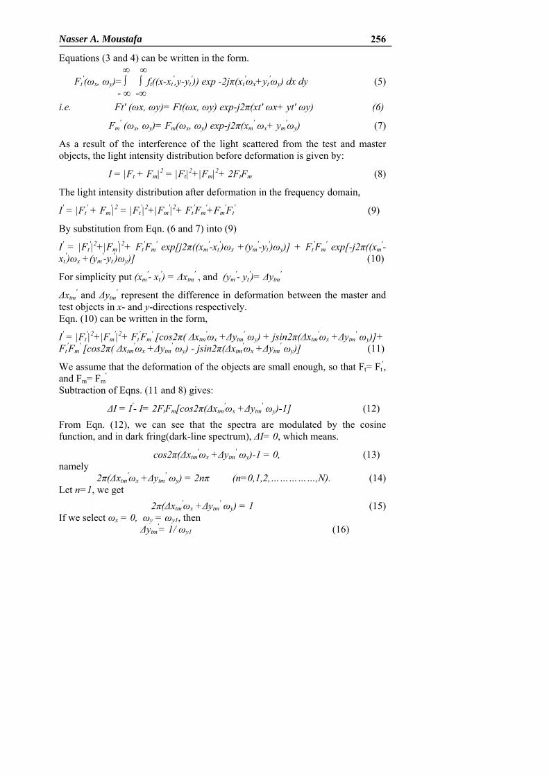
The optical system is presented schematically in Fig. (1). The incoming laser beam is divided by a beam splitter and is incident upon the two specimen surfaces after being steered by a set of mirrors. The two beams are adjusted so they are incident upon the two surfaces. The light diffused by the two specimens is superimposed by means of a beam splitter positioned between the imaging lens and the specimens. The speckle in the image plane resulted from the interference of the light diffused by the master and test specimens. The speckle interferograms are recorded by CCD camera and stored in the memory of a computer.

Fig.(1): The schematic of fringes in spectrum plane. In response to a deformation, the point Pm(x,y) on the surface of the

master specimen (before deformation) undergoes a displacement, so it moves to Pm

'(x-um, y-υm) after deformation. The companion point Pt(x,y) on the surface of the test specimen undergoes a displacement also, and moves to Pt

'(x-ut, y-υt). The displacement along x-direction being u(x,y), and the displacement along y-direction being υ(x,y).


As it is a micro-deformation, the points before and after deformation corresponds to each other. The light intensity of Pt(x,y) in the speckle image before deformation is equal to Pt

'(x-υt, y-υt) after deformation. Also the light intensity of Pm(x,y) before deformation is equal to Pm

'(x-um, y-υm) after deformation. ft(x,y), and ft

'(x,y), are used to express the light intensity functions of the speckle pattern of the surface of the test object before and after deformation respectively. fm(x,y) and fm

'(x,y), are used to express the light intensity functions of the speckle pattern of the surface of the master object before and after deformation respectively.

So, ft

'(x,y)=ft(x-ut, y- υt), and fm'(x,y)= fm(x-um, y- υm).

The Fourier transform of the two functions ft(x,y), and fm(x,y) for the test and master objects respectively before deformation are, ∞ ∞

Ft(ωx, ωy)= ∫ ∫ ft(x,y) exp -2jπ(xωx+yωy) dx dy (1) - ∞ -∞ and ∞ ∞

Fm(ωx, ωy)= ∫ ∫ fm(x,y) exp -2jπ(xωx+yωy) dx dy (2) - ∞ -∞ The Fourier transform of ft

'(x,y) and fm'(x,y).

∞ ∞ Ft

'(ωx, ωy)= ∫ ∫ ft'(x,y) exp -2jπ(xωx+yωy) dx dy

- ∞ -∞ ∞ ∞ = ∫ ∫ ft(x-ut,y-υt) exp -2jπ(xωx+yωy) dx dy (3) - ∞ -∞ ∞ ∞ and Fm

'(ωx, ωy)= ∫ ∫ fm'(x,y) exp -2jπ(xωx+yωy) dx dy

- ∞ -∞ ∞ ∞

= ∫ ∫ fm(x-um,y-υm) exp -2jπ(xωx+yωy) dx d (4) - ∞ -∞ when ut= xt

',υt= yt', um= xm

', and υm= ym' are constants along with the

displacement of the surface of the bodies, the light intensity function will change to ft(x-xt

', y-yt') and fm(x-xm

', y-ym'). (xt

', yt', and xm

', ym') indicates the

displacement along the x-axis and y-axis for the test and master objects, respectively.


Equations (3 and 4) can be written in the form. ∞ ∞

Ft'(ωx, ωy)= ∫ ∫ ft((x-xt

',y-yt')) exp -2jπ(xt

'ωx+yt'ωy) dx dy (5)

- ∞ -∞

i.e. Ft' (ωx, ωy)= Ft(ωx, ωy) exp-j2π(xt' ωx+ yt' ωy) (6)

Fm' (ωx, ωy)= Fm(ωx, ωy) exp-j2π(xm

' ωx+ ym'ωy) (7)

As a result of the interference of the light scattered from the test and master objects, the light intensity distribution before deformation is given by:

I = |Ft + Fm|2 = |Ft|2+|Fm|2+ 2FtFm (8)

The light intensity distribution after deformation in the frequency domain,

I' = |Ft' + Fm

'|2 = |Ft'|2+|Fm

'|2+ Ft'Fm

'+Fm'Ft

' (9)

By substitution from Eqn. (6 and 7) into (9)

I' = |Ft'|2+|Fm

'|2+ Ft'Fm

' exp[j2π((xm'-xt

')ωx +(ym'-yt

')ωy)] + Ft'Fm

' exp[-j2π((xm'-

xt')ωx +(ym

'-yt')ωy)] (10)

For simplicity put (xm'- xt

') = Δxtm' , and (ym

'- yt')= Δytm

'

Δxtm' and Δytm

' represent the difference in deformation between the master and test objects in x- and y-directions respectively. Eqn. (10) can be written in the form,

I' = |Ft'|2+|Fm

'|2+ Ft'Fm

' [cos2π( Δxtm'ωx +Δytm

' ωy) + jsin2π(Δxtm'ωx +Δytm

' ωy)]+ Ft

'Fm' [cos2π( Δxtm

'ωx +Δytm' ωy) - jsin2π(Δxtm

'ωx +Δytm' ωy)] (11)

We assume that the deformation of the objects are small enough, so that Ft= Ft',

and Fm= Fm'

Subtraction of Eqns. (11 and 8) gives:

ΔI = I'- I= 2FtFm[cos2π(Δxtm'ωx +Δytm

' ωy)-1] (12)

From Eqn. (12), we can see that the spectra are modulated by the cosine function, and in dark fring(dark-line spectrum), ΔI= 0, which means.

cos2π(Δxtm'ωx +Δytm

' ωy)-1 = 0, (13) namely

2π(Δxtm'ωx +Δytm

' ωy) = 2nπ (n=0,1,2,……………,N). (14) Let n=1, we get

2π(Δxtm'ωx +Δytm

' ωy) = 1 (15) If we select ωx = 0, ωy = ωy1, then Δytm

'= 1/ ωy1 (16)


If we select ωy = 0, ωx= ωx1, then

Δxtm'= 1/ ωy1 (17)

where ωx1 and ωy1 stands for the distances between the original points of coordinate and the crossing points, that is the first dark fringe intersects the coordinate axis (Fig. (2)).

Fig.(2): Setup for experimental speckle interferometry used to obtain fringes that contour the difference in displacements.

3. Experimental Validation.

To check the predictions of the discrete Fourier transform (DFT), the following experimental work was performed using the experimental arrangement in Fig. (1).

At first, the wave field scattered by the test object in its initial state and

the wave field scattered by the master object (undeformed) are superposed and recorded by CCD camera. Secondly the wave fields of the scattered wave of the master and test objects after deformation recorded also. The interferometric speckle pattern was stored as before. The two speckle patterns were subtracted from each other and the difference was displayed on the monitor as correlation fringes representing the difference in deformation. Discrete Fourier transform (DFT) made for the resulting image, and we get the fringe image in the spectral field.


The unit to be measured on the monitor is the pixel. So we must calibrate the magnification before the test. In this experiment, a distance of 2 μm of displacement along the x-direction in the space domain corresponds to 14 pixels on frequency axis.

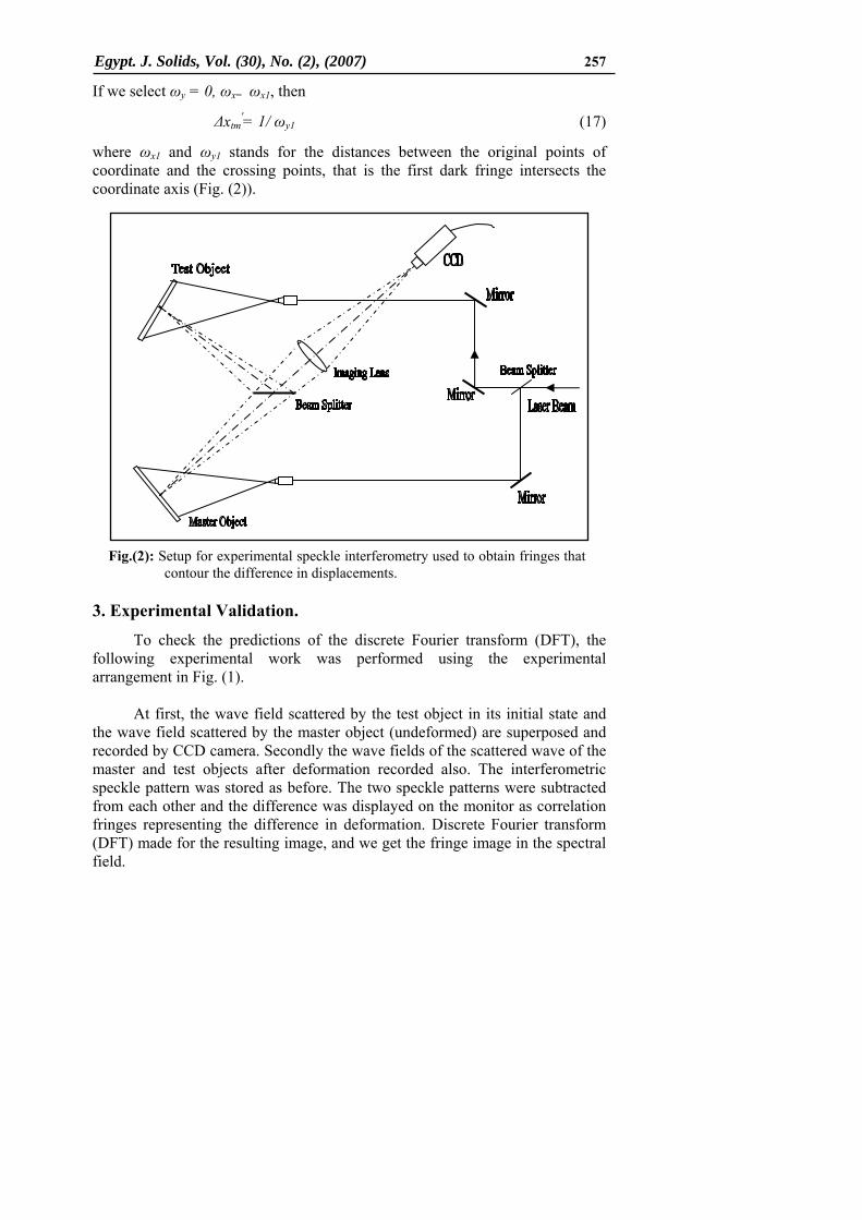
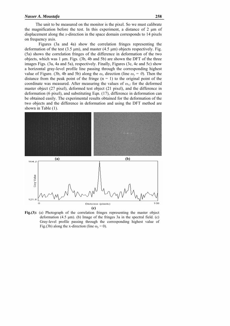
Figures (3a and 4a) show the correlation fringes representing the deformation of the test (3.5 μm), and master (4.5 μm) objects respectively. Fig. (5a) shows the correlation fringes of the difference in deformation of the two objects, which was 1 μm. Figs. (3b, 4b and 5b) are shown the DFT of the three images Figs. (3a, 4a and 5a), respectively. Finally, Figures (3c, 4c and 5c) show a horizontal gray-level profile line passing through the corresponding highest value of Figure. (3b, 4b and 5b) along the ωx direction (line ωy = 0). Then the distance from the peak point of the fringe (n = 1) to the original point of the coordinate was measured. After measuring the values of ωx1 for the deformed master object (27 pixel), deformed test object (21 pixel), and the difference in deformation (6 pixel), and substituting Eqn. (17), difference in deformation can be obtained easily. The experimental results obtained for the deformation of the two objects and the difference in deformation and using the DFT method are shown in Table (1).

(b) (a)

(c) Fig.(3): (a) Photograph of the correlation fringes representing the master object

deformation (4.5 μm). (b) Image of the fringes 3a in the spectral field. (c) Gray-level profile passing through the corresponding highest value of Fig.(3b) along the x-direction (line ωy = 0).


(b) (a)

(c)

Fig.(4): (a) Photograph of the correlation fringes representing the test object deformation (3.5 μm). (b) Image of the fringes 4a in the spectral field. (c) Gray-level profile passing through the corresponding highest value of Fig.4b along the x-direction (line ωy=0).

Table (1): Results of Experiment.

ent by micrometer (μm)

Relative error

DisplacemDisplacement by DFT (μm)

0.048 4.5 4.29 Master 0.047 3.5 3.34 Test 0.052 1 0.95 Difference


(b) (a)

(c)

Fig.(5): (a) Photograph of the correlation fringes representing the difference correlation fringes (1 μm). (b) Image of the fringes 5a in the spectral field. (c) Gray-level profile passing through the corresponding highest of value Fig.5b along the x-direction (line ωy=0).

From the Table (1) we can see, the good agreement achieved between the experimental results and the results obtained by the DFT method.

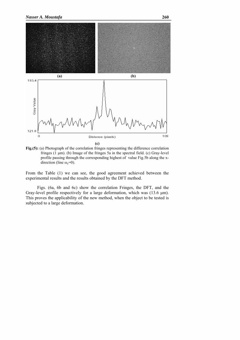
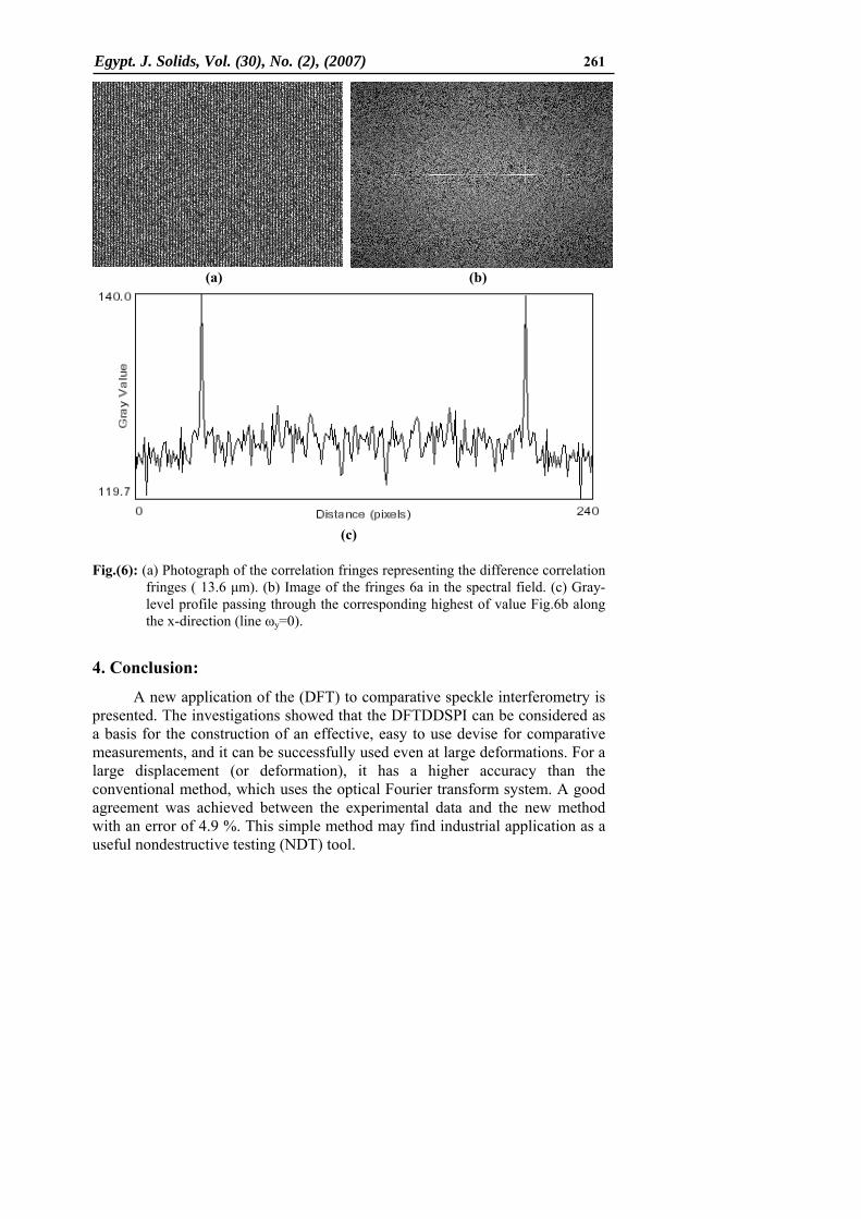
Figs. (6a, 6b and 6c) show the correlation Fringes, the DFT, and the Gray-level profile respectively for a large deformation, which was (13.6 μm). This proves the applicability of the new method, when the object to be tested is subjected to a large deformation.


(b) (a)

(c)

Fig.(6): (a) Photograph of the correlation fringes representing the difference correlation

fringes ( 13.6 μm). (b) Image of the fringes 6a in the spectral field. (c) Gray-level profile passing through the corresponding highest of value Fig.6b along the x-direction (line ωy=0).

4. Conclusion:

A new application of the (DFT) to comparative speckle interferometry is presented. The investigations showed that the DFTDDSPI can be considered as a basis for the construction of an effective, easy to use devise for comparative measurements, and it can be successfully used even at large deformations. For a large displacement (or deformation), it has a higher accuracy than the conventional method, which uses the optical Fourier transform system. A good agreement was achieved between the experimental data and the new method with an error of 4.9 %. This simple method may find industrial application as a useful nondestructive testing (NDT) tool.


5. References:

1. M. Takeda, H.Ina and K. Kobayashy, J. Opt. Soc. Am.72 (1), 1566 (1982). 2. M. Takeda, Indust. Metr. 1 (2), 79 (1990). 3. M. Takeda and M. Mutoh, Appl. Opt. 22 (23), 3977 (1983). 4. M. Takeda and Z. Tung, J. Opt. 16 (1), 127 (1985). 5. M. Takeda and K. Kabayashy, Appl. Opt. 23 (11), 1760 (1984). 6. M. Suemastu and M. Takeda, Appl. Opt. 30 (28), 1760 (1991). 7. T. Kreis, J. Opt. Soc. Am, 3 (6), 847 (1986). 8. Zhang Yuanpeng, Exp. Mech., 42 (1), 18 (2002). 9. Nasser A. Moustafa, János Kornis, Opt. Commu., 172, 9 (1999). 10. Nasser A. Moustafa, János Kornis, Zöltan Füzessy, Opt. Eng. 38(7), 1241

(July 1999). 11. A. R. Ganesan, C. Joenathan and R. S. Sirohi, Opt. Commu., 64 (6), 501

(1987).

comparative measurement in speckle interferometry using ...egmrs.powweb.com/ejs/pdf/vol302/8.pdf ·...

Documents