comparative analysis of the hydraulic parameters of … · abstract—the present paper presents...
TRANSCRIPT

Abstract— The present paper presents the comparative analysis of the hydraulic parameters, respectively flow rate and pressure, determined on a physical model and also calculated by the use of the automatic program for steady flow, RIMIS. The physical model was developed by the authors for the study of motion in a water distribution looped network. The comparative analysis aims the validation of the RIMIS program created by the authors. The experimental results are destined for the analysis of the steady motion, as a reference for transitory motion in a ring type pipe network, for possible operating situations.
Keywords— physical modeling, ring type pipe network, steady water motion.
I. INTRODUCTION
HE complexity of the water motion phenomenon in distribution networks, the assumptions and restrictions
from diverse equations governing the motion sometimes reveal uncertainties on the sphere of applicability or on the limits of these equations [3, 5].
The goal of our research was the analyze of the physical phenomenon of water motion in looped networks using special conceived software packs and furthermore, the validation of the software on the basis of experimental measurements on a laboratory stand that models the physical phenomenon [4].
Steps in research conducting: � design of an automatic calculation program for modeling
the water motion phenomenon in steady flows in a distribution network.
� design and construction of an experimental stand for physical modeling of a loop in a water distribution network.
M. Stănescu is with is with “Ovidius” University from Constanta,
Romania; Faculty of Civil Engineering, Department of Hydraulic Structures (e-mail: [email protected]).
A. Constantin is with “Ovidius” University from Constanta, Romania; Faculty of Civil Engineering, Department of Hydraulic Structures, (e-mail: [email protected]).
C. St. Nitescu is with “Ovidius” University from Constanta, Romania; Faculty of Civil Engineering, Department of Hydraulic Structures (e-mail: [email protected]).
L. Roşu is with “Ovidius” University from Constanta, Romania; Faculty of Civil Engineering, Department of Hydraulic Structures (e-mail: [email protected]).
A. M. Dobre is student at Constanta Maritime University, Romania; Faculty of Navigation and Naval Transport (e-mail: [email protected]).
� simulation of possible situations that can occur while operating looped water distribution networks.
� comparison of the results obtained by automatic calculation to the results from experimental measurements.
II. PROBLEM FORMULATION
A. Theoretical basis of the analyzed problem
For looped pipe networks: � the following elements are assumed known: land
configuration; flow supply in nodes; pressure in the supply nodes.
� the following are determined: flow rates in sides of the looped network; pressures in the network nodes.
If the network has [8]: � b independent loops; � n nodes; � s sides,
Euler’s equation is valid:
1−+= bns (1) For the 2s variables (pressures and flows) the following
equations can be written: � the continuity equation in nodes (representing n-1
equations):
0=∑n
nQ (2)
where the flow rate sum, Qn, is performed algebraically considering, by convention:
� positive, the ingoing flows in the analyzed node; � negative, the outgoing flows from the analyzed node.
� hydraulic pressure loss equations for loops (b equations):
0=∑s
rsh (3)
where the pressure loss sum, hrs, is performed algebraically considering, by convention:
� positive, the hydraulic pressure loss on the pipe sections in which the flow direction is the same as the
Comparative analysis of the hydraulic parameters of steady water flow in a looped
pipe network
Mădălina Stănescu, Anca Constantin, Claudiu Şt. NiŃescu, Lucica Roşu and Adrian Mihai Dobre
T
INTERNATIONAL JOURNAL OF MATHEMATICAL MODELS AND METHODS IN APPLIED SCIENCES
Issue 8, Volume 5, 2011 1301

chosen theoretical direction (clockwise); � negative, the hydraulic pressure loss on the pipe
sections in which the flow direction is opposite to the chosen theoretical direction (counterclockwise).
Pressure loss (hr) [1]:
rlocrlin hh +=rh (4)
Linear pressure loss (hrlin) according to the Darcy equation:
2g
v
D
lλh
2
intlinr ⋅⋅= (5)
where:
λλλλ – Darcy hydraulic resistance coefficient; l – length of the pipe section, [m]; Dint – inner diameter of the pipe section, [m]; v – water velocity in pipes, [m/s]; g – gravitational acceleration, [m/s2]; k – absolute roughness, [m]. Local pressure loss (hrloc) is generated by flow disturbances,
flow control parts, elbows, tees, reducers, characterized by the local pressure loss coefficient, ζζζζ.
2g
vζh
2
locr ⋅= (6)
Local pressure loss, hrloc, can be equated with linear loss on
additional sections of equivalent length, ∆lv [8]. The following condition is fulfilled:
λζ
∆ intDlv
⋅= (7)
It is known that the pressure loss (hr) can also be determined
from:
2rh QM ⋅= (8)
where:
M – the hydraulic resistance modulus, [s2/m5]; Q – flow rate in pipe section, [m3/s]. The hydraulic resistance modulus, M, calculation formula
taking into consideration the linear pressure loss (5), and the local pressure loss (6) is:
⋅+⋅⋅
⋅⋅=
4int
5int
2
1
D
lλ
2
16M
Dgζ
π (9)
The Reynolds number, Re, calculation formula is:
υintDv
Re⋅
= (10)
where υ – cinematic water viscosity, [m2/s].
According to the Reynolds criterion there is a critical value, Recr, depending on which the flow regimes are divided in:
2300ReRe =< cr - laminar flow regime;
2300ReRe => cr - turbulent flow regime.
The calculation of the Darcy hydraulic resistance coefficient
depends on the flow regime, as follows: - for laminar flow, Poiseuille equation is recommended:
Re
64λ = (11)
- for turbulent flow regime, the differentiation is made using
the Moody criterion.
0int
λD
kReM ⋅⋅=o (12)
a) smooth regime, 14<Mo ⇒
6-0,35 103Re,Re61,000071, ⋅<+=λ (13)
b) transition regime, 00214 ≤≤ Mo ⇒
+−=
λ
ε
λ Re
51,2
7,3ln86,0
1
intD (14)
c) fully rough regime, 002>Mo ⇒
85int 10Re10 1.138,k
Dlg2
λ
1<<+⋅= (15)
Returning to the set of equations (1), (2) and (3), used in the
calculation of the looped networks, it is found that a number of s equations with 2n variables is obtained. A practical method of solving the problem, which is undetermined from mathematical and hydraulic points of view, is the Hardy-Cross method (1946) [6]. The method consists of the following steps:
a) Rational flow directions are chosen in the pipe sections of the network and their size is estimated so that the continuity equations in nodes are satisfied. A general procedure of achieving this consists of choosing the loop flow rates by analogy with the electrical contour currents.
b) In order to satisfy the hydraulic pressure loss equations in
INTERNATIONAL JOURNAL OF MATHEMATICAL MODELS AND METHODS IN APPLIED SCIENCES
Issue 8, Volume 5, 2011 1302
loops, a flow correction equation, ∆Q, is introduced on each contour.
Admitting that the practical hydraulic pressure loss equation for a certain section is
n
r QMh ⋅= (16)
and the chosen flow rate is Q0, for which
∑ ≠⋅ 00nQM (17)
The following condition is required:
0)( 0 =+=⋅= ∑∑∑ nnr QQMQMh ∆ (18)
If the correction flows ∆Q are considered small, from the
previous condition, through linearization, it is deduced that:
∑∑
−⋅⋅
⋅=
10
0
n
n
QMn
QMQ∆ (19)
for the considered loop. The sign of a correction ∆Q is kept the same for all the sides of the loop, and it algebraically summed with the flow rate in each side (this is the reason why the absolute value is introduced on the denominator).
c) the corrected flows are calculated for all the contour sections and the method is repeated until the desired precision is achieved. Usually, it is required that:
� mhr 0005.0<∆ in any loop and
� mhr 0005.0)( max <∆ on the entire network.
B. Physical model description
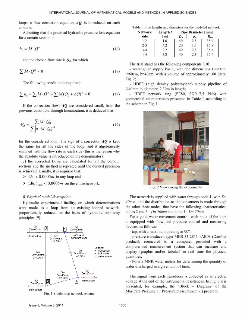
Hydraulic experimental facility, on which determinations were made, is a loop from an existing looped network, proportionally reduced on the basis of hydraulic similarity principles [9].
Fig. 1 Single loop network scheme
Table I. Pipe lengths and diameters for the modeled network
Network side
Length l [m]
Pipe Diameter [mm]
Dn en Dint 1-2 1,0 40 2,3 35,4 2-3 4,2 20 1,6 16,8 3-4 2,2 40 2,3 35,4 1-4 3,8 40 2,3 35,4
The trial stand has the following components [10]: - rectangular supply basin, with the dimensions L=90cm,
l=60cm, h=40cm, with a volume of approximately 160 liters, Fig. 2;
- HDPE (high density polyethylene) supply pipeline of Ø40mm in diameter, 2.30m in length;
- HDPE network ring (PE80, SDR17,5 PN6) with geometrical characteristics presented in Table I, according to the scheme in Fig. 1.
Fig. 2 View during the experiments
The network is supplied with water through node 1, with Dn
40mm, and the distribution to the consumers is made through the other three nodes, that have the following characteristics: nodes 2 and 3 - Dn 40mm and node 4 - Dn 20mm.
For a good water movement control, each node of the loop is equipped with flow and pressure control and measuring devices, as follows:
- tap, with a maximum opening at 90º; - pressure transducer, type MBS 33-2811-1AB08 (Danfoss
product), connected to a computer provided with a computerized measurement system that can measure and display (graphic and/or tabular) in real time the physical quantities;
- Polaris MNK water meters for determining the quantity of water discharged in a given unit of time.
The signal from each transducer is collected as an electric
voltage at the end of the instrumental resistances. In Fig. 3 it is presented, for example, the “Block – Diagram” of the Măsurare Presiune.vi (Pressure measurement.vi) program.
INTERNATIONAL JOURNAL OF MATHEMATICAL MODELS AND METHODS IN APPLIED SCIENCES
Issue 8, Volume 5, 2011 1303

Fig. 3 Block – Diagram of the Pressure Measurement.vi program
For the 7 maneuvering methods of the three water delivery
valves, with the 4 opening situations, 30°, 45°, 60° and 90°, the hydraulic characteristics of the pipe sections are determined.
In order to establish the flow on each section, the Darcy hydraulic resistance coefficient, λ, is determined through successive approximations, as a calculation refinement: � The first approximation step, in which, for each section of
the analyzed looped network, the hydraulic resistance modulus, flow rate, water velocity and the Reynolds number are calculated as a function of the average value of
the Darcy hydraulic resistance coefficient, 02,0λ 0 =
(Table II); � The second approximation step, in which the hydraulic
resistance modulus, flow, water velocity and the Reynolds number on each pipe section are calculated as a function of the Darcy hydraulic resistance coefficient, λ, calculated on the basis of the Reynolds number from the first approximation step (Table III).
The hydraulic resistance modulus, water velocity, Reynolds
number, Moody number and Darcy hydraulic resistance coefficient are determined on the basis of the calculation equations previously presented.
According to the obtained results, the flow regime is defined on each pipe section, for all the analyzed cases, whatever would be the opening angle of the maneuvered valves.
For example, the flow regime calculation is presented in
Table II and Table III, for all valves opened, N2+N3+N4.
C. Steady water motion automatic calculation program for
looped pipe networks – “RIMIS”
The looped pipe network dimensioning problems solving demanded the development of an automatic calculation program that meets the following requirements:
- easy management of several types of projects; - input, edit and easy modification of the input data. - obtaining reports, used in graphic representation and in
interpreting the results. The automatic calculation program- RIMIS, Turbo Pascal
language designed, allows the modeling of the steady water motion phenomenon in a distribution network, supplied by constant level reservoirs or by pumping stations [8].
INTERNATIONAL JOURNAL OF MATHEMATICAL MODELS AND METHODS IN APPLIED SCIENCES
Issue 8, Volume 5, 2011 1304

Table II Reynolds number and flow regime determination – valves in nodes N2+N3+N4 opened (first approximation)
Opening angle,
α [°°°°]
Ring section
L [m]
D [m]
ζζζζ
First approximation
Observation λ
M [s2/m5]
Q [l/s]
v [m/s]
Re Mo
30
1-2 1 0,0354 0,6 0,020 92.833,51 0,469 0,477 20.842,40 0,83 Smooth flow 2-3 4,2 0,0168 1,04 0,020 7.092.494,74 0,049 0,223 4.620,40 0,39 Smooth flow 3-4 2,2 0,0354 0,7 0,020 181.090,71 0,271 0,275 12.016,54 0,48 Smooth flow 1-4 3,8 0,0354 1 0,020 191.818,27 0,357 0,363 15.864,88 0,63 Smooth flow
45
1-2 1 0,0354 0,6 0,020 92.833,51 0,822 0,835 36.514,31 1,46 Smooth flow 2-3 4,2 0,0168 1,04 0,020 7.092.494,74 0,097 0,439 9.105,87 0,77 Smooth flow 3-4 2,2 0,0354 0,7 0,020 181.090,71 0,509 0,518 22.616,98 0,90 Smooth flow 1-4 3,8 0,0354 1 0,020 191.818,27 0,658 0,668 29.203,57 1,17 Smooth flow
60
1-2 1 0,0354 0,6 0,020 92.833,51 1,059 1,076 47.013,42 1,88 Smooth flow 2-3 4,2 0,0168 1,04 0,020 7.092.494,74 0,120 0,540 11.205,97 0,94 Smooth flow 3-4 2,2 0,0354 0,7 0,020 181.090,71 0,640 0,650 28.402,29 1,13 Smooth flow 1-4 3,8 0,0354 1 0,020 191.818,27 0,829 0,842 36.794,64 1,47 Smooth flow
90
1-2 1 0,0354 0,6 0,020 92.833,51 1,220 1,239 54.160,95 2,16 Smooth flow 2-3 4,2 0,0168 1,04 0,020 7.092.494,74 0,120 0,540 11.202,78 0,94 Smooth flow 3-4 2,2 0,0354 0,7 0,020 181.090,71 0,688 0,699 30.547,03 1,22 Smooth flow 1-4 3,8 0,0354 1 0,020 191.818,27 0,896 0,911 39.797,86 1,59 Smooth flow
Tabel III Reynolds number and flow regime determination – valves in nodes N2+N3+N4 opened (second approximation)
Opening angle,
α [°°°°]
Ring section
L [m]
D [m]
ζζζζ
Second approximation
Observation λ
M [s2/m5]
Q [l/s]
v [m/s]
Re Mo
30
1-2 1 0,0354 0,6 0,019 92.075,91 0,465 0,472 20.641,21 0,81 Smooth flow 2-3 4,2 0,0168 1,04 0,033 10.340.474,75 0,045 0,202 4.196,47 0,45 Smooth flow 3-4 2,2 0,0354 0,7 0,023 192.473,63 0,275 0,280 12.217,73 0,53 Smooth flow 1-4 3,8 0,0354 1 0,021 199.565,93 0,362 0,368 16.066,07 0,66 Smooth flow
45
1-2 1 0,0354 0,6 0,016 87.103,65 0,814 0,827 36.152,78 1,30 Smooth flow 2-3 4,2 0,0168 1,04 0,026 8.597.020,23 0,089 0,402 8.344,07 0,80 Smooth flow 3-4 2,2 0,0354 0,7 0,019 177.693,22 0,517 0,526 22.978,51 0,89 Smooth flow 1-4 3,8 0,0354 1 0,017 177.132,14 0,666 0,676 29.565,10 1,10 Smooth flow
60
1-2 1 0,0354 0,6 0,015 85.162,37 1,049 1,066 46.582,46 1,60 Smooth flow 2-3 4,2 0,0168 1,04 0,024 8.141.280,36 0,110 0,497 10.297,87 0,95 Smooth flow 3-4 2,2 0,0354 0,7 0,018 173.122,01 0,649 0,660 28.833,25 1,08 Smooth flow 1-4 3,8 0,0354 1 0,016 169.811,87 0,838 0,852 37.225,60 1,33 Smooth flow
90
1-2 1 0,0354 0,6 0,014 84.147,97 1,210 1,229 53.717,05 1,81 Smooth flow 2-3 4,2 0,0168 1,04 0,024 8.141.881,81 0,110 0,495 10.267,42 0,95 Smooth flow 3-4 2,2 0,0354 0,7 0,017 171.736,19 0,698 0,709 30.990,94 1,15 Smooth flow 1-4 3,8 0,0354 1 0,016 167.457,78 0,906 0,921 40.241,76 1,42 Smooth flow
The operating mode is described on an application on a
single loop network (Fig. 4), which has the geometrical characteristics of the physical model.
The program does not require a special rule for node and side numbering.
For achieving the above presented objectives, the RIMIS
program was designed in three main modules.
Fig. 4 Scheme of the looped network used as an application for the
RIMIS program
INTERNATIONAL JOURNAL OF MATHEMATICAL MODELS AND METHODS IN APPLIED SCIENCES
Issue 8, Volume 5, 2011 1305

a. “Input” module Initially, preliminary flow estimation is made for the
network sides in order to meet the continuity conditions in nodes and to assure the imposed discharge flows in some nodes. For the determination of the initial flow on each pipe section of the looped network of the physical model, each case is analyzed taking into account the chosen flow direction, the chosen theoretical direction (clockwise) and the diameter of the pipe sections.
The initial section flow is tabular presented. The values of the initial flow rate on each section are presented in Table IV, for the case: all valves opened, N2+N3+N4.
Table IV Initial flow on each section, all valves opened, N2+N3+N4
Opening angle, α
[°°°°]
Initial flow, Q [l/s]
Tr. 1-2 Tr. 2-3 Tr. 3-4 Tr. 1-4
30 0,484 0,064 0,256 0,343 45 0,846 0,121 0,485 0,634 60 1,091 0,152 0,608 0,797 90 1,262 0,162 0,646 0,854
The automatic calculation program will determine the pressures in the network nodes as a function of the water pressure from the supply source (constant level water tank), situated in the node N1, and the delivered flow rates in the network nodes in the simulated opening versions of the valves.
Input data for the calculation of the analyzed network are
saved in a file having the extension ***.inp. A screenshot of the file hrdcrs25.inp for one of the analyzed cases, all valves opened at an angle α = 30º, is presented in Fig. 5.
All the other analyzed versions correspond to different valve
maneuvering cases: - as a function of the valve opening angle, α (respectively
30º, 45º, 60º and 90º) - as a function of the number of opened valves.
Fig. 5 RIMIS program input data file
b. “Calculation Program” module This module is composed of the following steps for solving
the dimensioning problems of networks operating in steady flow [2]:
- correction of the initial flow rate using successive iterations alongside the network loops until the value of the maximum imposed flow rate error is achieved, using the Hardy-Cross method;
- flow rate calculation on each pipeline section of the network;
- analysis of the chosen routes for the calculation of the piezometric load;
- calculation of the piezometric load in each node. c. “Result Presentation” module Upon running the program, based on the input data from the
***.inp file, reports are edited with output data in a file with the extension ***.out. A screenshot of the file hrdcrs25.out for the analyzed case, is presented in Fig. 6.
The result file contains: � the display of the initial data from the input file; � flow corrections evolution in calculation iterations; � final values of the flow rate in the loop sides; � pressure values in the component nodes of the selected
piezometric lines. The obtained values in the case: all valves opened,
N2+N3+N4, are provided in Table V.
Tabel V Calculated parameters, all valves opened, N2+N3+N4
Opening angle, α
[°°°°]
Calculated flow, Q [l/s] Piezometric load, p [mCA]
Tr. 1-2 Tr. 2-3 Tr. 3-4 Tr. 1-4 Node 1 Node 2 Node 3 Node 4
30 0,464 0,044 0,276 0,363 1,756 1,736 1,713 1,729 45 0,811 0,086 0,520 0,669 1,756 1,706 1,636 1,682 60 1,046 0,107 0,653 0,842 1,756 1,680 1,579 1,647 90 1,208 0,108 0,700 0,908 1,756 1,660 1,557 1,632
INTERNATIONAL JOURNAL OF MATHEMATICAL MODELS AND METHODS IN APPLIED SCIENCES
Issue 8, Volume 5, 2011 1306

Fig. 6 RIMIS program output data file
III. COMPARATIVE ANALYSIS OF THE CALCULATED AND
EXPERIMENTAL RESULTS
Different valve operating modes were analyzed, each representing a possible operating case of the distribution network, for example, the simultaneous opening of all the taps, N2+N3+N4.
In all simulated cases, the taps were operated at different opening angles α, respectively 30º, 45º, 60º and 90º.
Simultaneously, in all cases, pressure and flow rate readings were made.
The research was done in two main directions: - determination of flow rate on each pipeline section of the
analyzed network, in steady operating conditions. - pressure determination in each node, as an average of the
pressures measured during the steady flow.
A. Comparative flow rate analysis
In Table VI there are presented the flow rate values obtained either on the physical model or using the RIMIS program, in the case: all taps opened, N2+N3+N4.
Table VI The flow rate for each side of the loop, as a function of the
opening angle of the taps. All taps opened N2+N3+N4.
α
[°]
Flow rate [l/s] Tr. 1-2 Tr. 2-3 Tr. 3-4 Tr. 1-4
Model RIMIS Model RIMIS Model RIMIS Model RIMIS
30 0,465 0,464 0,045 0,044 0,275 0,276 0,362 0,363
45 0,814 0,811 0,089 0,086 0,517 0,520 0,666 0,669
60 1,049 1,046 0,110 0,107 0,649 0,653 0,838 0,842
90 1,210 1,208 0,110 0,108 0,698 0,700 0,906 0,908
A more intuitive representation of these data is graphically made, in Fig. 7 ÷ Fig. 10, for each section of the loop.
Fig. 7 Comparative analysis of the flow rate on 1-2 section as a
function of the opening angle of the taps
Fig. 8 Comparative analysis of the flow rate on 2-3 section as a
function of the opening angle of the taps
INTERNATIONAL JOURNAL OF MATHEMATICAL MODELS AND METHODS IN APPLIED SCIENCES
Issue 8, Volume 5, 2011 1307
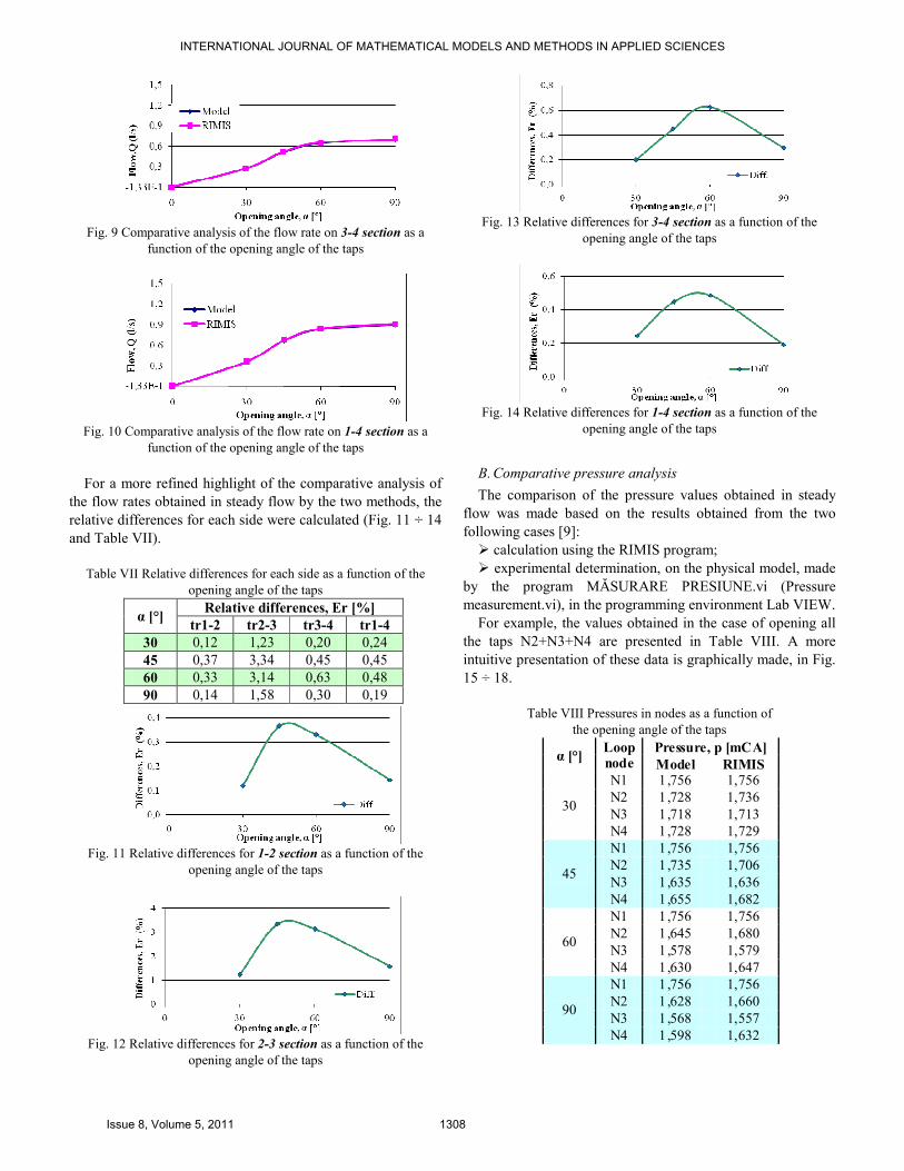
Fig. 9 Comparative analysis of the flow rate on 3-4 section as a
function of the opening angle of the taps
Fig. 10 Comparative analysis of the flow rate on 1-4 section as a
function of the opening angle of the taps For a more refined highlight of the comparative analysis of
the flow rates obtained in steady flow by the two methods, the relative differences for each side were calculated (Fig. 11 ÷ 14 and Table VII).
Table VII Relative differences for each side as a function of the
opening angle of the taps
α [°] Relative differences, Er [%]
tr1-2 tr2-3 tr3-4 tr1-4
30 0,12 1,23 0,20 0,24 45 0,37 3,34 0,45 0,45 60 0,33 3,14 0,63 0,48 90 0,14 1,58 0,30 0,19
Fig. 11 Relative differences for 1-2 section as a function of the
opening angle of the taps
Fig. 12 Relative differences for 2-3 section as a function of the
opening angle of the taps
Fig. 13 Relative differences for 3-4 section as a function of the
opening angle of the taps
Fig. 14 Relative differences for 1-4 section as a function of the
opening angle of the taps
B. Comparative pressure analysis
The comparison of the pressure values obtained in steady flow was made based on the results obtained from the two following cases [9]:
� calculation using the RIMIS program; � experimental determination, on the physical model, made
by the program MĂSURARE PRESIUNE.vi (Pressure measurement.vi), in the programming environment Lab VIEW.
For example, the values obtained in the case of opening all the taps N2+N3+N4 are presented in Table VIII. A more intuitive presentation of these data is graphically made, in Fig. 15 ÷ 18.
Table VIII Pressures in nodes as a function of
the opening angle of the taps
α [°] Loop node
Pressure, p [mCA]
Model RIMIS
30
N1 1,756 1,756 N2 1,728 1,736 N3 1,718 1,713 N4 1,728 1,729
45
N1 1,756 1,756 N2 1,735 1,706 N3 1,635 1,636 N4 1,655 1,682
60
N1 1,756 1,756 N2 1,645 1,680 N3 1,578 1,579 N4 1,630 1,647
90
N1 1,756 1,756 N2 1,628 1,660 N3 1,568 1,557 N4 1,598 1,632
INTERNATIONAL JOURNAL OF MATHEMATICAL MODELS AND METHODS IN APPLIED SCIENCES
Issue 8, Volume 5, 2011 1308

Fig. 15 Comparative analysis of pressures in nodes, α=30°
Fig. 16 Comparative analysis of pressures in nodes, α=45°
Fig. 17 Comparative analysis of pressures in nodes, α=60°
Fig. 18 Comparative analysis of pressures in nodes, α=90°
IV. CONCLUSION
The study focused on looped networks, frequently used in water distribution systems and also in industrial or irrigation installations. The experimental measurements validated the results obtained by the use of the RIMIS program.
� The RIMIS program, written in a TURBO PASCAL language, designed for modeling the steady water motion in a distribution network, provides reports on flow rate and pressure values in an entire loop; it allows an easy comparison of these values of pressure and flow rate to the ones obtained on the experimental stand.
� The program models with good accuracy the water flow through the sides of the loop whether the flow is laminar or turbulent. The regime of flow is determined on the basis of the Reynolds criterion and the Moody criterion.
� The small values of the relative errors allow us to validate the automate program RIMIS, with respect to the flow rates on the sides of the single loop network and the pressures in the network nodes.
In conclusion, the program is useful for a single loop in a distribution network and it can be extended to a network with multiple loops.
The precision pointed out by the comparison of theoretical and experimental results reveals that the RIMIS program is a useful instrument for experts interested in the simulation of water flow in a network to be designed.
REFERENCES
[1] D.I. Arsenie, “Hydraulics, hydrology, hydrogeology” - vol.1, Constanta, 1977.
[2] I. Bartha, V. Javgureanu, “Hydraulics”, vol, 1, Editura Tehnică, Chişinău, 1998.
[3] A. Bărbulescu, V. Marza, Electrical effect induced at the boundary of an acoustic cavitation zone, Acta Physica Polonica B, vol.37, no. 2, 2006, pp. 507 – 518
[4] S. Hâncu, G. Marin, “Theoretical and applied hydraulics”, vol. I şi II, Editura Cartea Universitară, Bucureşti, 2007.
[5] C. Koncsag, A. Bărbulescu, Modeling the removal of mercaptans from liquid hydrocarbon streams in structured packing columns, Chemical Engineering and Processing, 47, Issues 9-10, 2008, pp.1717 - 1725
[6] A. Mănescu, “Water supply. Examples of calculation”, Ed. HGA, Bucureşti, 1998.
[7] M. Popescu, D.I. Arsenie, P. Vlase, “Applied hydraulic transients for hydropower plants and pumping stations”, Balkema Publishers, Lisse, Abington, Tokyo, 2004.
[8] I. Seteanu, V. Rădulescu, N. Vasiliu, D. Vasiliu, “Fluid mechanics and hydraulics. Fundamentals and applications”, Editura Tehnică, Bucureşti, 1998.
[9] M. Stănescu, A. Constantin, C. Bucur, A. Stănescu, L. Roşu, “Experimental stand for the study of unsteady water flow through pipelines and pile networks”, Scientific Bulletin of the „Politehnica” University of Timişoara, Transactions on Hydrotechnics, Vol. 55 (69), No. 1-2, Timişoara, Romania, 2010, pp. 211–219.
[10] M. Stănescu, A. Constantin, C.Şt. NiŃescu, L. Roşu, A.M. Dobre “Research on the steady motion in water distribution looped pipe networks”, Recent researches in computational techniques, non-linear systems and control, Published by WSEAS Press, ISBN: 978-1-61804-011-4, Iasi, Romania, July 1-3, 2011, pp. 243–246.
Mădălina Stănescu was born in Constanta, Romania, in 1979. She graduated in civil engineering at “Ovidius” University of Constanta, Romania, in 2003 and took her PhD degree in civil engineering at The Faculty of Civil Engineering, “Ovidius” University Constanta , in 2010. She worked as a designer engineer, and since 2004 she has been teaching at “Ovidius” University, Constanta, The Faculty of Civil Engineering. She published over 12 scientific articles. Her research field is fluid mechanics and applied hydraulics.
INTERNATIONAL JOURNAL OF MATHEMATICAL MODELS AND METHODS IN APPLIED SCIENCES
Issue 8, Volume 5, 2011 1309