cmb observations and results dmitry pogosyan university of alberta lake louise, february, 2003...
TRANSCRIPT

CMB observations and results
Dmitry Pogosyan
University of Alberta
Lake Louise, February, 2003
•Lecture 1: What can Cosmic Microwave Background tell us about the Universe ? A theoretical introduction.
•Lecture 2: Recent successes in the mapping of CMB anisotropy: what pre-WMAP and WMAP data reveals.

É T=T(nê) =P
`a`mY?`m(nê)
∆T/T ~ 10-5
C` = hja2`mji

Sachs-WolfeEffect
Acoustic Oscillations
Drag
Damping
Curvature`pk ø R ?=rs(ñ?)
Òbh2
ø eà (`=̀D)mD
Doppler
Tensors
Reionizationø eà2üc
Phenomenology of the Angular Power Spectrum
Òbh2;Òdmh2
large <-- scales --> small

Error origins – noise and ‘cosmic variance’
Cosmic Variance ~ Cl / √fsky Noise

Relikt, 1983 (USSR)
• First CMB anisotropy data actively used to restrict cosmological models
• Quadrupole dT/T < 4 x 10⁻⁵
• Many models where dismissed for failing this limit – hot (massive neutrino) dark matter, late
decaying neutrinos ….

COBE-DMR, 1992 First detection of anisotropy large angular scale l < 20 growing initial slope ns=1.20.2 Low quadrupole power

Search for the first acoustic peak:• TOCO 1998• Boomerang NAmerica, 1997

Mapping acoustic oscillations:• Boomerang 2000-2002• Maxima 2000-2001• DASI 2001

2002CBI – damping tailArcheops – low l link to COBEACBAR - medium-high lDASI – detection of polarization

Pre WMAP parameters (Jan 2003)


Deficiencies
• Covering only part of the sky leads to high cosmic variance uncertainties. (Noise is not an issue at l < 1000)
• Patched coverage of the angular scales enhances role of systematics (e.g., calibration and beam uncertainties) which dominates analysis.
• As the result – limited success of breaking some degeneracies c – 8 as predicted from CMB
c – ns
c – gravitational waves


Wilkinson Microwave Probe (WMAP) – launch June 2001, first year data release – Feb 11, 2003
•75-85% of full sky•5 frequency channels at 23-94 Ghz• First 1year data – sky is covered twice•Each pixel observed ~3000 times. Cosmic variance limited up to l~600 •0.5% calibration uncertainty

WMAP high S/N, high resolution CMB map of the full sky

Joint pre-WMAPk= -0.05 0.05
b = 0.022 0.002cdm = 0.12 0.02ns = 0.95 0.04
c < 0.3-0.4
WMAPextk= -0.02 0.02
b = 0.0224 0.0009 cdm = 0.135 0.009
h = 0.71 0.04
ns = runs 1.2-0.93 c = 0.17 0.04
WMAP alonek= -0.03 0.05
b = 0.024 0.001 cdm = 0.14 0.02
h = 0.72 0.05
ns = 0.99 0.04 c= 0.15 0.07
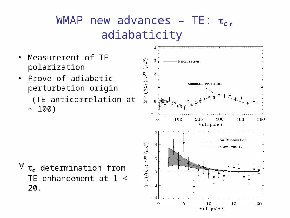
• Measurement of TE polarization
• Prove of adiabatic perturbation origin
(TE anticorrelation at ~ 100)
c determination from TE enhancement at l < 20.
WMAP new advances – TE: c, adiabaticity

CMB Polarization
• Full description of radiation is by polarization matrix, not just intensity – Stockes parameters, I,Q,U,V
• Why would black-body radiation be polarized ? Well, it is not in equilibrium, it is frozen with Plankian spectrum, after last Thompson scattering, which is a polarizing process.
• But only, because there is local quadrupole anisotropy of the photon flux scattered of electron. Thus, P and dT/T are intimately related, second sources first (there is back-reaction as well).
• There is no circular polarization generated, just linear – Q,U. Level of polarization ~10% for scalar perturbations, factor of 10 less for
tensors. Thus needed measurements are at dT/T~10-6 – 10-8 level.
• As field on the sky – B, E modes (think vectors, but in application to second rank tensor), distinguished by parity.


WMAP new advances – extending the parameter list
• Do we need ever precise determination of the parameters ? Yes, if we want to explore larger parameter space.,
• WMAP:– Running ns – positive slope
at low l, negative at higher l Recall COBE-DMR, it also preferred n~1.2 ! Also, low quadrupole – hint to new physics ?
– Gravitational wave (tensor) contribution to dT/T is small < 0.72 of scalar component


“The Seven Pillars” of the CMB(of inflationary adiabatic fluctuations)
Large Scale Anisotropies
Acoustic Peaks/Dips
Gaussianity
Polarization, TE correlation
Damping Tail
•Secondary Anisotropies
•Gravity Waves, B-type polarization pattern
Minimal Inflationary parameter set
Quintessesnce
Tensor fluc.
Broken Scale Invariance

BOOMERANG
Cosmic Background Imager (CBI)
ACBAR