climate: observations, projections and impacts: russia
TRANSCRIPT
Climate: Observations, projections and impacts: Russia Met Office Simon N. Gosling, University of Nottingham Robert Dunn, Met Office Fiona Carrol, Met Office Nikos Christidis, Met Office John Fullwood, Met Office Diogo de Gusmao, Met Office Nicola Golding, Met Office Lizzie Good, Met Office Trish Hall, Met Office Lizzie Kendon, Met Office John Kennedy, Met Office Kirsty Lewis, Met Office Rachel McCarthy, Met Office Carol McSweeney, Met Office Colin Morice, Met Office David Parker, Met Office Matthew Perry, Met Office Peter Stott, Met Office Kate Willett, Met Office Myles Allen, University of Oxford Nigel Arnell, Walker Institute, University of Reading Dan Bernie, Met Office Richard Betts, Met Office Niel Bowerman, Centre for Ecology and Hydrology Bastiaan Brak, University of Leeds John Caesar, Met Office Andy Challinor, University of Leeds Rutger Dankers, Met Office Fiona Hewer, Fiona's Red Kite Chris Huntingford, Centre for Ecology and Hydrology Alan Jenkins, Centre for Ecology and Hydrology Nick Klingaman, Walker Institute, University of Reading Kirsty Lewis, Met Office Ben Lloyd-Hughes, Walker Institute, University of Reading Jason Lowe, Met Office Rachel McCarthy, Met Office James Miller, Centre for Ecology and Hydrology Robert Nicholls, University of Southampton Maria Noguer, Walker Institute, University of Reading Friedreike Otto, Centre for Ecology and Hydrology Paul van der Linden, Met Office Rachel Warren, University of East Anglia The country reports were written by a range of climate researchers, chosen for their subject expertise, who were drawn from institutes across the UK. Authors from the Met Office and the University of Nottingham collated the contributions in to a coherent narrative which was then reviewed. The authors and contributors of the reports are as above.
Developed at the request of:
Research conducted by:
Russia
Climate: Observations, projections and impacts

We have reached a critical year in our response to climate change. The decisions that we made in Cancún put the UNFCCC process back on track, saw us agree to limit temperature rise to 2 °C and set us in the right direction for reaching a climate change deal to achieve this. However, we still have considerable work to do and I believe that key economies and major emitters have a leadership role in ensuring a successful outcome in Durban and beyond. To help us articulate a meaningful response to climate change, I believe that it is important to have a robust scientific assessment of the likely impacts on individual countries across the globe. This report demonstrates that the risks of a changing climate are wide-ranging and that no country will be left untouched by climate change. I thank the UK’s Met Office Hadley Centre for their hard work in putting together such a comprehensive piece of work. I also thank the scientists and officials from the countries included in this project for their interest and valuable advice in putting it together. I hope this report will inform this key debate on one of the greatest threats to humanity.
The Rt Hon. Chris Huhne MP, Secretary of State for Energy and Climate Change
There is already strong scientific evidence that the climate has changed and will continue to change in future in response to human activities. Across the world, this is already being felt as changes to the local weather that people experience every day.
Our ability to provide useful information to help everyone understand how their environment has changed, and plan for future, is improving all the time. But there is still a long way to go. These reports – led by the Met Office Hadley Centre in collaboration with many institutes and scientists around the world – aim to provide useful, up to date and impartial information, based on the best climate science now available. This new scientific material will also contribute to the next assessment from the Intergovernmental Panel on Climate Change.
However, we must also remember that while we can provide a lot of useful information, a great many uncertainties remain. That’s why I have put in place a long-term strategy at the Met Office to work ever more closely with scientists across the world. Together, we’ll look for ways to combine more and better observations of the real world with improved computer models of the weather and climate; which, over time, will lead to even more detailed and confident advice being issued.
Julia Slingo, Met Office Chief Scientist

IntroductionUnderstanding the potential impacts of climate change is essential for informing both adaptation
strategies and actions to avoid dangerous levels of climate change. A range of valuable national
studies have been carried out and published, and the Intergovernmental Panel on Climate Change
(IPCC) has collated and reported impacts at the global and regional scales. But assessing the
LPSDFWV�LV�VFLHQWL¿FDOO\�FKDOOHQJLQJ�DQG�KDV��XQWLO�QRZ��EHHQ�IUDJPHQWHG��7R�GDWH��RQO\�D�OLPLWHG�amount of information about past climate change and its future impacts has been available at
QDWLRQDO�OHYHO��ZKLOH�DSSURDFKHV�WR�WKH�VFLHQFH�LWVHOI�KDYH�YDULHG�EHWZHHQ�FRXQWULHV��
,Q�$SULO�������WKH�0HW�2I¿FH�+DGOH\�&HQWUH�ZDV�DVNHG�E\�WKH�8QLWHG�.LQJGRP¶V�6HFUHWDU\�RI�6WDWH�IRU�(QHUJ\�DQG�&OLPDWH�&KDQJH�WR�FRPSLOH�VFLHQWL¿FDOO\�UREXVW�DQG�LPSDUWLDO�LQIRUPDWLRQ�RQ�WKH�SK\VLFDO�LPSDFWV�RI�FOLPDWH�FKDQJH�IRU�PRUH�WKDQ����FRXQWULHV��7KLV�ZDV�GRQH�XVLQJ�D�FRQVLVWHQW�VHW�RI�VFHQDULRV�DQG�DV�D�SLORW�WR�D�PRUH�FRPSUHKHQVLYH�VWXG\�RI�FOLPDWH�LPSDFWV��$�UHSRUW�RQ�WKH�REVHUYDWLRQV��SURMHFWLRQV�DQG�LPSDFWV�RI�FOLPDWH�FKDQJH�KDV�EHHQ�SUHSDUHG�IRU�HDFK�FRXQWU\��7KHVH�SURYLGH�XS�WR�GDWH�VFLHQFH�RQ�KRZ�WKH�FOLPDWH�KDV�DOUHDG\�FKDQJHG�DQG�WKH�SRWHQWLDO�FRQVHTXHQFHV�RI�IXWXUH�FKDQJHV��7KHVH�UHSRUWV�FRPSOHPHQW�WKRVH�SXEOLVKHG�E\�WKH�,3&&�DV�ZHOO�DV�WKH�PRUH�GHWDLOHG�FOLPDWH�FKDQJH�DQG�LPSDFW�VWXGLHV�SXEOLVKHG�QDWLRQDOO\��
Each report contains:
���$�GHVFULSWLRQ�RI�NH\�IHDWXUHV�RI�QDWLRQDO�ZHDWKHU�DQG�FOLPDWH��LQFOXGLQJ�DQ�DQDO\VLV�RI�QHZ� data on extreme events.
���$Q�DVVHVVPHQW�RI�WKH�H[WHQW�WR�ZKLFK�LQFUHDVHV�LQ�JUHHQKRXVH�JDVHV�DQG�DHURVROV�LQ�WKH�DWPRVSKHUH�KDYH�DOWHUHG�WKH�SUREDELOLW\�RI�SDUWLFXODU�VHDVRQDO�WHPSHUDWXUHV�FRPSDUHG�WR� SUH�LQGXVWULDO�WLPHV��XVLQJ�D�WHFKQLTXH�FDOOHG�µIUDFWLRQ�RI�DWWULEXWDEOH�ULVN�
���$�SUHGLFWLRQ�RI�IXWXUH�FOLPDWH�FRQGLWLRQV��EDVHG�RQ�WKH�FOLPDWH�PRGHO�SURMHFWLRQV�XVHG�LQ�WKH� Fourth Assessment Report from the IPCC.
���7KH�SRWHQWLDO�LPSDFWV�RI�FOLPDWH�FKDQJH��EDVHG�RQ�UHVXOWV�IURP�WKH�8.¶V�$YRLGLQJ� Dangerous Climate Change programme (AVOID) and supporting literature.
)RU�GHWDLOV�YLVLW��KWWS���ZZZ�DYRLG�XN�QHW
7KH�DVVHVVPHQW�RI�LPSDFWV�DW�WKH�QDWLRQDO�OHYHO��ERWK�IRU�WKH�$92,'�SURJUDPPH�UHVXOWV�DQG�WKH�FLWHG�VXSSRUWLQJ�OLWHUDWXUH��ZHUH�PRVWO\�EDVHG�RQ�JOREDO�VWXGLHV��7KLV�ZDV�WR�HQVXUH�FRQVLVWHQF\��ZKLOVW�UHFRJQLVLQJ�WKDW�WKLV�PLJKW�QRW�DOZD\V�SURYLGH�HQRXJK�IRFXV�RQ�LPSDFWV�RI�PRVW�UHOHYDQFH�WR�D�SDUWLFXODU�FRXQWU\��$OWKRXJK�WLPH�DYDLODEOH�IRU�WKH�SURMHFW�ZDV�VKRUW��JHQHUDOO\�DOO�WKH�PDWHULDO�DYDLODEOH�WR�WKH�UHVHDUFKHUV�LQ�WKH�SURMHFW�ZDV�XVHG��XQOHVV�WKHUH�ZHUH�JRRG�VFLHQWL¿F�UHDVRQV�IRU�QRW�GRLQJ�VR��)RU�H[DPSOH��VRPH�LPSDFWV�DUHDV�ZHUH�RPLWWHG��VXFK�DV�PDQ\�RI�WKRVH�DVVRFLDWHG�ZLWK�KXPDQ�KHDOWK��,Q�WKLV�FDVH��WKHVH�LPSDFWV�DUH�VWURQJO\�GHSHQGDQW�RQ�ORFDO�IDFWRUV�DQG�GR�QRW�HDVLO\�OHQG�WKHPVHOYHV�WR�WKH�JOREDOO\�FRQVLVWHQW�IUDPHZRUN�XVHG��1R�DWWHPSW�ZDV�PDGH�WR�LQFOXGH�WKH�HIIHFW�RI�IXWXUH�DGDSWDWLRQ�DFWLRQV�LQ�WKH�DVVHVVPHQW�RI�SRWHQWLDO�LPSDFWV��7\SLFDOO\��VRPH��EXW�QRW�DOO��RI�WKH�LPSDFWV�DUH�DYRLGHG�E\�OLPLWLQJ�JOREDO�DYHUDJH�ZDUPLQJ�WR�QR�PRUH�WKDQ����&��
7KH�0HW�2I¿FH�+DGOH\�&HQWUH�JUDWHIXOO\�DFNQRZOHGJHV�WKH�LQSXW�WKDW�RUJDQLVDWLRQV�DQG�LQGLYLGXDOV�IURP�WKHVH�FRXQWULHV�KDYH�FRQWULEXWHG�WR�WKLV�VWXG\���0DQ\�QDWLRQV�FRQWULEXWHG�UHIHUHQFHV�WR�WKH�OLWHUDWXUH�DQDO\VLV�FRPSRQHQW�RI�WKH�SURMHFW�DQG�KHOSHG�WR�UHYLHZ�HDUOLHU�YHUVLRQV�RI�WKHVH�UHSRUWV��
:H�ZHOFRPH�IHHGEDFN�DQG�H[SHFW�WKHVH�UHSRUWV�WR�HYROYH�RYHU�WLPH��)RU�WKH�ODWHVW�YHUVLRQ�RI�WKLV�UHSRUW��GHWDLOV�RI�KRZ�WR�UHIHUHQFH�LW��DQG�WR�SURYLGH�IHHGEDFN�WR�WKH�SURMHFW�WHDP��SOHDVH�VHH�WKH�ZHEVLWH�DW�ZZZ�PHWRI¿FH�JRY�XN�FOLPDWH�FKDQJH�SROLF\�UHOHYDQW�REV�SURMHFWLRQV�LPSDFWV
,Q�WKH�ORQJHU�WHUP��ZH�ZRXOG�ZHOFRPH�WKH�RSSRUWXQLW\�WR�H[SORUH�ZLWK�RWKHU�FRXQWULHV�DQG�RUJDQLVDWLRQV�RSWLRQV�IRU�WDNLQJ�IRUZDUG�DVVHVVPHQWV�RI�QDWLRQDO�OHYHO�FOLPDWH�FKDQJH�LPSDFWV�through international cooperation.


1
Summary
Climate observations
x There has been widespread warming over Russia since 1960 with increases in the
frequency of warm days and nights and decreases in the frequency of cool days and
nights.
x There is evidence for a general increase in seasonal temperatures averaged over the
country as a result of human influence on climate, making the occurrence of warm
seasonal temperatures more frequent and cold seasonal temperatures less frequent.
x Between 1960 and 2003, over western Russia there has been a widespread increase
in annual total precipitation.
Climate change projections
x For the A1B emissions scenario projected changes in temperature are higher over
northern parts of the country, with increases of above 5.5°C in the Arctic regions. In
central parts of the country, increases range between around 4.5-5.5°C, and in
southern and western regions, increases lie in the range of 3.5-4°C. There is
moderate agreement between the CMIP3 models over most of Russia.
x The CMIP3 models project that precipitation will increase over almost the entire
country. Increases of above 20% are projected in the north of the country, with most
other regions projected to experience increases of between 10% and 20%. In the
Caucasus region, projected precipitation change ranges from an increase of 5% to a
decrease of 5%. Agreement between the CMIP3 model is high over most of the
country, but more moderate in parts of the southwest.
Climate change impacts projections
Crop yields
x Whilst a definitive conclusion on the impact of climate change on crop yields in
Russia cannot be drawn, the majority of global- and regional-scale studies included in
this report project a decrease in the yield of wheat, Russia’s major crop, as a
consequence of climate change.

2
x Studies from the AVOID programme suggest a mixed outcome, with some areas of
cultivated land becoming more suitable for agriculture, and other areas becoming less
suitable, as a result of climate change.
Food security
x Russia is currently a country with extremely low levels of undernourishment. The
majority of global- and regional-scale studies included here project that although
negatively affected, the country is unlikely to face severe food security issues over
the next 40 years as a consequence of climate change.
x National-scale assessments are consistent in showing that climate change could
have a negative impact on food security in Russia.
Water stress and drought
x Global-scale studies included here show that the west of Russia is the most
vulnerable region of the country to water stress. For the rest of the country and
particularly the east, vulnerability is presently low.
x The majority of global-scale studies included here project an increase in water stress
across the country as a whole with climate change, although there is regional
variation.
x However, recent simulations from the AVOID programme show consensus across
models for little change in the population exposed to increased or decreased water
stress with climate change.
Pluvial flooding and rainfall
x Recent studies suggest that winter precipitation could increase for Russia under
climate change, and there is consistency across different climate models in this
change.
x Increases in precipitation from extreme storm events are also possible with climate
change, although it is not possible to directly translate these into detailed pluvial flood
projections.

3
Fluvial flooding
x Recent studies have suggested that flood magnitudes for Central and Eastern Siberia
and the Russian Far East may increase with climate change, but decrease in
European Russia and West Siberia, due to smaller maximum rates of snowmelt
runoff.
x Results from simulations by the AVOID programme, show, a high level of agreement
among climate models, that flood risk across Russia as a whole could decrease with
climate change throughout the 21st century.
x Although most studies present a useful indicator of exposure to flood risk with climate
change, none of them account for the effect that hydropower reservoirs, present in
most large rivers, can have on the height of the annual flood peak, which can be
substantial. Also, few studies have investigated the occurrence of ice dams and the
potential resultant flooding with climate change.
Coastal regions
x There is very little work on the impact of climate change on Russia’s coastal regions,
however one study estimates that the population exposure to sea level rise (SLR)
could increase from 189,000 in present to 226,000 under un-mitigated A1B emissions
in 2070. Relative to A1B an aggressive mitigation policy could avoid an exposure of
around 28,000 people by 2070.

4

5
Table of contents Chapter 1 – Climate Observations ........................................................................ 7��Rationale ................................................................................................................................. 8�Climate overview .................................................................................................................. 10�
Analysis of long-term features in the mean temperature .................................................... 11�Temperature extremes ........................................................................................................ 13�
Recent extreme temperature events .................................................................................. 14�Extreme Siberian winter, December 2000-February 2001 ............................................. 14�Cold spell, January 2006 ................................................................................................ 15�Heat wave, July-August 2010 ........................................................................................ 15�
Analysis of long-term features in moderate temperature extremes .................................... 15�Attribution of changes in likelihood of occurrence of seasonal mean temperatures ........... 21�
Winter 2000/01 ............................................................................................................... 21�Winter 2005/06 ............................................................................................................... 21�Summer 2010................................................................................................................. 22�
Precipitation extremes ........................................................................................................ 24�Recent extreme precipitation events .................................................................................. 26�
Flooding, June 2002....................................................................................................... 26�Drought, August 2008 .................................................................................................... 26�
Analysis of precipitation extremes from 1960 ..................................................................... 26�Summary ............................................................................................................................... 31�Methodology annex ............................................................................................................. 32�
Recent, notable extremes ................................................................................................... 32�Observational record .......................................................................................................... 33�
Analysis of seasonal mean temperature ........................................................................ 33�Analysis of temperature and precipitation extremes using indices ................................ 34�Presentation of extremes of temperature and precipitation ........................................... 43�
Attribution ............................................................................................................................ 46�References ............................................................................................................................ 49�Acknowledgements ............................................................................................................. 53�Chapter 2 – Climate Change Projections ........................................................ 55�Introduction .......................................................................................................................... 56�Climate projections .............................................................................................................. 58�
Summary of temperature change in Russia ....................................................................... 59�Summary of precipitation change in Russia ....................................................................... 59�
Chapter 3 – Climate Change Impact Projections ........................................ 61�Introduction .......................................................................................................................... 62�
Aims and approach ............................................................................................................. 62�Impact sectors considered and methods ............................................................................ 62�Supporting literature ........................................................................................................... 63�AVOID programme results .................................................................................................. 63�Uncertainty in climate change impact assessment ............................................................. 64�
Summary of findings for each sector ................................................................................ 69�Crop yields ........................................................................................................................... 72�
Headline .............................................................................................................................. 72�Supporting literature ........................................................................................................... 72�
Introduction .................................................................................................................... 72�Assessments that include a global or regional perspective ........................................... 73�National-scale or sub-national scale assessments ........................................................ 77�
AVOID programme results .................................................................................................. 79�

6
Methodology................................................................................................................... 79�Results ........................................................................................................................... 80�
Food security ....................................................................................................................... 82�Headline .............................................................................................................................. 82�Supporting literature ........................................................................................................... 82�
Introduction .................................................................................................................... 82�Assessments that include a global or regional perspective ........................................... 83�National-scale or sub-national scale assessments ........................................................ 93�
Water stress and drought ................................................................................................... 97�Headline .............................................................................................................................. 97�Supporting literature ........................................................................................................... 97�
Introduction .................................................................................................................... 97�Assessments that include a global or regional perspective ........................................... 98�National-scale or sub-national scale assessments ...................................................... 107�
AVOID Programme Results .............................................................................................. 109�Methodology................................................................................................................. 109�
Pluvial flooding and rainfall .............................................................................................. 111�Headline ............................................................................................................................ 111�Supporting literature ......................................................................................................... 111�
Introduction .................................................................................................................. 111�Assessments that include a global or regional perspective ......................................... 111�National-scale or sub-national scale assessments ...................................................... 112�
Fluvial flooding .................................................................................................................. 114�Headline ............................................................................................................................ 114�Supporting literature ......................................................................................................... 114�
Introduction .................................................................................................................. 114�Assessments that include a global or regional perspective ......................................... 115�National-scale or sub-national scale assessments ...................................................... 117�
AVOID programme results ................................................................................................ 117�Methodology................................................................................................................. 117�Results ......................................................................................................................... 118�
Tropical cyclones ............................................................................................................... 120�Coastal regions .................................................................................................................. 121�
Headline ............................................................................................................................ 121�Assessments that include a global or regional perspective ......................................... 121�National-scale or sub-national scale assessments ...................................................... 127�
References .......................................................................................................................... 128�

7
Chapter 1 – Climate Observations �
�
�
�
�

8
Rationale
Present day weather and
climate play a fundamental
role in the day to day running
of society. Seasonal
phenomena may be
advantageous and depended
upon for sectors such as
farming or tourism. Other
events, especially extreme
ones, can sometimes have
serious negative impacts posing risks to life and infrastructure, and significant cost to the
economy. Understanding the frequency and magnitude of these phenomena, when they
pose risks or when they can be advantageous and for which sectors of society, can
significantly improve societal resilience. In a changing climate it is highly valuable to
understand possible future changes in both potentially hazardous events and those
reoccurring seasonal events that are depended upon by sectors such as agriculture and
tourism. However, in order to put potential future changes in context, the present day must
first be well understood both in terms of common seasonal phenomena and extremes.
The purpose of this chapter is to summarise the weather and climate from 1960 to present
day. This begins with a general climate overview including an up to date analysis of changes
in surface mean temperature. These changes may be the result of a number of factors
including climate change, natural variability and changes in land use. There is then a focus
on extremes of temperature and precipitation selected from 2000 onwards, reported in the
World Meteorological Organization (WMO) Annual Statement on the Status of the Global
Climate and/or the Bulletin of the American Meteorological Society (BAMS) State of the
Climate reports. This is followed by a discussion of changes in moderate extremes from
1960 onwards using an updated version of the HadEX extremes database (Alexander et al.,
2006) which categorises extremes of temperature and precipitation. These are core climate
variables which have received significant effort from the climate research community in
terms of data acquisition and processing and for which it is possible to produce long high
quality records for monitoring. For seasonal temperature extremes, an attribution analysis
then puts the seasons with highlighted extreme events into context of the recent climate
versus a hypothetical climate in the absence of anthropogenic emissions (Christidis et al.,
Figure 1. Location of boxes for the regional average time series (red dashed box) in Figures 2 and 3 and the attribution region (grey box) in Figures 4, 5 and 6.

9
2011). It is important to note that we carry out our attribution analyses on seasonal mean
temperatures over the entire country. Therefore these analyses do not attempt to attribute
the changed likelihood of individual extreme events. The relationship between extreme
events and the large scale mean temperature is likely to be complex, potentially being
influenced by inter alia circulation changes, a greater expression of natural internal variability
at smaller scales, and local processes and feedbacks. Attribution of individual extreme
events is an area of developing science. The work presented here is the foundation of future
plans to systematically address the region’s present and projected future weather and
climate and the associated impacts.
The methodology section that follows provides details of the data shown here and of the
scientific analyses underlying the discussions of changes in the mean temperature and in
temperature and precipitation extremes. It also explains the methods used to attribute the
likelihood of occurrence of seasonal mean temperatures.

10
Climate overview
The most well known feature of the Russian climate is its very cold winter, brought about by
the country’s high latitudes (40-75°N), vast land mass and lack of any topographic
obstructions to protect it from arctic winds sweeping across its long, north-facing and often
frozen coastline. The country is bounded by high mountains along its southern and eastern
flank but the west is exposed to occasional winter incursions of milder Atlantic air, so that
winters become progressively more severe eastwards. Average daily maximum
temperatures along, approximately, the 55°N line of latitude in January are -6°C in Moscow
(longitude 38°E), -11°C at Chelyabinsk (61°E), -12°C at Novosibirsk (84°E) and -14°C at
Irkutsk (105°E), with even lower values further north. During the winter, an intense area of
high pressure develops over particularly the Asian part of Russia, with intensely cold air
spiralling out from it to affect countries well beyond Russia’s boundaries.
However, the extreme continental nature of the Russian climate means that the difference
between mid-winter and mid-summer monthly mean temperature is large and typically at
least 30°C, so that summers are warm even, for a short time, within the Arctic Circle. For
instance coastal Archangel’sk at 64.5°N has typical July daily maxima of 21°C. In southern
Russia, and in some years elsewhere, summer is hot – e.g. Astrakhan, at 46°N near the
Caspian Sea, has typical July daily maxima of 31-32°C. Annual mean temperatures are,
nonetheless, quite low, for instance (in a north-south line from 65°N to 46°N) 1°C at
Archangelsk, 5°C at Moscow and 10°C at Astrakhan. The transition from winter to summer
and from summer back to winter is very quick so that effectively there are only 2 seasons
over most of Russia.
Annual precipitation is mostly not particularly high and is spread throughout the year with a
summer convective peak. Examples of annual average precipitation are 690mm at Moscow
but only 400-500 mm further east at Chelybinsk, Novosibirsk and Irkutsk. Annual average
precipitation typically becomes very low towards the most southerly parts of Russia, for
instance only 213 mm at Astrakhan. A small portion of Russia along its eastern (Pacific)
seaboard, characterised by Vladivostock, has rather more rainfall in summer, brought about
by the Asian summer monsoon in which low pressure develops over the heated land mass
of Asia and causes moist winds to blow onshore. Most winter precipitation in Russia falls as
snow but this, though frequent, is rarely very heavy and strong winds often sweep the
ground bare of snow.

11
In the north and east of Siberia (Asiatic Russia) a phenomenon known as permafrost occurs
in which the subsoil remains frozen all year, causing special issues to the construction
industry, even though the topsoil thaws in summer. Other weather hazards in Russia include
floods and extremes of heat and cold.
Analysis of long-term features in the mean temperature
CRUTEM3 data (Brohan et al., 2006) have been used to provide an analysis of mean
temperatures from 1960 to 2010 over Russia using the median of pairwise slopes method to
fit the trend (Sen, 1968; Lanzante, 1996). The methods are fully described in the
methodology section. In agreement with increasing global average temperatures (Sánchez-
Lugo et al., 2011), over the period 1960 to 2010 there is a geographically widespread
warming signal over Russia as shown in Figure 2, consistent with previous research
(UNFCCC, 2010). Grid boxes in which the 5th to 95th percentiles of the slopes are of the
same sign can be more confidently regarded as showing a signal different to zero trend.
There is higher confidence in this warming signal for a number of grid boxes in summer
(June to August), mostly towards the south. For winter (December to February) confidence
in the grid box signals is lower for the majority of grid boxes. There are few data over the
northern and eastern regions. Here, cooling is shown in winter but there is lower confidence
in this signal. Regionally averaged trends (over grid boxes included in the red dashed box in
Figure 1) calculated by the median of pairwise slopes show warming signals but with lower
confidence. For winter this is 0.35 oC per decade (5th to 95th percentile of slopes: -0.08 to
0.71 oC per decade) and for summer this is 0.11 oC per decade (5th to 95th percentile of
slopes: -0.01 to 0.23 oC per decade).
12
Figu
re 2
. Dec
adal
tren
ds in
sea
sona
lly a
vera
ged
tem
pera
ture
s fo
r Rus
sia
and
the
surr
ound
ing
regi
ons
over
the
perio
d 19
60 to
201
0. M
onth
ly m
ean
anom
alie
s fro
m C
RU
TEM
3 (B
roha
n et
al.,
200
6) a
re a
vera
ged
over
eac
h 3
mon
th s
easo
n (J
une-
July
-Aug
ust –
JJA
and
Dec
embe
r-Ja
nuar
y-Fe
brua
ry –
DJF
). Tr
ends
are
fitte
d us
ing
the
med
ian
of p
airw
ise
slop
es m
etho
d (S
en, 1
968;
Lan
zant
e, 1
996)
. The
re is
hig
h co
nfid
ence
in th
e tre
nds
show
n if
the
5th to
95th
pe
rcen
tiles
of t
he p
airw
ise
slop
es d
o no
t enc
ompa
ss z
ero
beca
use
here
the
trend
is c
onsi
dere
d to
be
sign
ifica
ntly
diff
eren
t fro
m a
zer
o tre
nd (n
o ch
ange
). Th
is is
sho
wn
by a
bla
ck d
ot in
the
cent
re o
f the
resp
ectiv
e gr
id-b
ox.

13
Temperature extremes
Both hot and cold temperature extremes can place many demands on society. While
seasonal changes in temperature are normal and indeed important for a number of societal
sectors (e.g. tourism, farming etc.), extreme heat or cold can have serious negative impacts.
Importantly, what is ‘normal’ for one region may be extreme for another region that is less
well adapted to such temperatures.
Table 1 shows extreme events since 2000 that are reported in WMO Statements on Status
of the Global Climate and/or BAMS State of the Climate reports. Two periods of extreme
cold, the winters of 2001 and 2006, and one of extreme heat, summer 2010, are highlighted
below as examples of recent extreme temperature events that have affected Russia.
Year Month Event Details Source
2000 May Cold Western regions experienced temperatures 4-5 °C colder than normal. WMO (2001)
2001 Dec ‘00-Feb ‘01 Cold
Siberia/Mongolia/E Russia had a severe winter, with temperatures dropping to -60 °C in January. WMO (2002)
2002 Jan-Feb Warm
In S. Siberia temperatures were up to 10 °C higher than normal in January. Across SE Siberia warm records were broken in February.
BAMS (Bulygina et al., 2003)
2002 Dec Cold Central and southern European Russia experienced the coldest mean monthly temperature in 70 years.
BAMS (Bulygina et al., 2003)
2003 Jan Cold In NW Russia temperatures dropped to -45 °C. WMO (2004)
2003 Jun Cold
European Russia experienced one of coldest Junes in 100 years. Lowest ever June temperatures recorded at some stations, with June temperatures typically 3-4 °C lower than normal.
BAMS (Bulygina, 2004)
2005 Feb Cold Republic of Tuva had the most severe frosts in 20 years. Temperatures dropped to -48 °C.
BAMS (Bulygina et al., 2006)
2005 Mar Cold European Russia experienced record cold monthly means in some places.
BAMS (Bulygina et al., 2006)
2005 May Heat Ural Federal District had the warmest May in 105 years.
BAMS (Bulygina et al., 2006)

14
(Table 1 continued)
Year Month Event Details Source
2005 Jul Heat wave
Western and southern-central regions of Siberia recorded temperatures reaching 39 °C.
BAMS (Bulygina et al., 2006)
2006 Jan Cold
Western Russian Federation experienced the coldest Moscow temperatures for 30 years. Western Siberia had record-breaking low monthly mean temperatures. Lowest temperatures across Russia reached -58.5 °C.
WMO (2007), BAMS (Bulygina et al., 2007)
2006 Aug Heat wave
Southern Federal District recorded temperatures reaching 37–43 °C.
BAMS (Bulygina et al., 2007)
2007 May Heat wave
The highest temperatures recorded in Moscow since 1891. Temperatures reached 38-39 °C in the Volgograd Region and north of the Astrakhan Region.
WMO (2008), BAMS (Bulgina et al., 2008)
2008 Aug Heat wave
Southern European Russia recorded maximum temperatures exceeding 30 °C for 24-25 days. Highest temperatures reached 36-40 °C.
BAMS (Bulgina et al., 2009)
2009 Feb Cold Russian Federation recorded temperatures 3-6 °C colder than normal. WMO (2009)
2009 Jul Heat wave
European Russia recorded air temperatures of 40-42 °C in Volgograd and Astrakhan regions.
BAMS (Bulgina et al., 2010)
2010 Jun-Aug Heat wave
Hottest summer on record. Most extreme in western Russia. Moscow had record high temperature of 38.2 °C. WMO (2011)
Table 1. Extreme temperature events reported in WMO Statements on Status of the Global Climate and/or BAMS State of the Climate reports since 2000.
Recent extreme temperature events
Extreme Siberian winter, December 2000-February 2001
Siberia, the far east of Russia, and Mongolia experienced a particularly severe winter
season. The anomalously cold conditions began in November and, for Siberia, this was the
coldest November-January period for 30 years (Waple et al., 2002). In January, Some areas
in central and southern Siberia experienced minimum temperatures of -60 °C (WMO, 2002).
High energy demand and fuel prices led to power cuts, and cold-related illnesses, such as
frostbite and hypothermia, were more common than usual (Waple et al., 2002). The cold
conditions were not confined to Siberia and temperatures were reported to be more than

15
3 °C colder than normal across much of Russia; in Moscow, hypothermia resulted in more
than 100 deaths (WMO, 2002).
Cold spell, January 2006
During the early part of 2006, much of Russia experienced very cold temperatures and
severe frosts. Monthly mean low temperature records were broken in parts of western
Siberia. Nationwide, the lowest temperature recorded was -58.5 °C on 30th January in the
Evenki Autonomous Area (Bulygina et al., 2007). January 2006 also saw Moscow
experience its coldest temperatures in 30 years (WMO, 2007).
Heat wave, July-August 2010
From early July through to the first half of August western Russia experienced an intense
heat wave, having already been subject to significantly above average temperature in the
previous 2 months. In Moscow, temperatures were 7.6 °C above average for July, making it
the hottest July on record by 2 °C. On 29th July, Moscow recorded its hottest ever
temperature of 38.2 °C. There were also 33 consecutive days above 30 °C in the city (WMO,
2011). Around 14,000 deaths resulted from the summer heat, with half of them in and
around Moscow alone (Maier et al., 2011).
The heat was accompanied by destructive forest fires, leaving thousands of people
homeless. The wildfires combined with the severe drought conditions, particularly in the
Volga region, led to widespread crop failures, where over 20% of Russian crops were
destroyed. Economic losses amounted to US$15 billion (WMO, 2011; Maier et al., 2011).
Analysis of long-term features in moderate temperature extremes
ECA&D data (Klein Tank et al., 2002) have been used to update the HadEX extremes
analysis for Russia from 1960 to 2010 using daily maximum and minimum temperatures.
Here we discuss changes in the frequency of cool days and nights and warm days and
nights which are moderate extremes. Cool days/nights are defined as being below the 10th
percentile of daily maximum/minimum temperature and warm days/nights are defined as
being above the 90th percentile of the daily maximum/minimum temperature. The methods
are fully described in the methodology section.
Between 1960 and 2009, there have been widespread increases in the frequency of warm
days/nights and decreases in the frequency of cool days/nights, in agreement with warming

16
mean temperature (Figure 3) and previous research (UNFCCC, 2010). There is high
confidence that this signal is different to zero for a high proportion of grid boxes, especially
for the nights. The data presented here are annual totals, averaged across all seasons, and
so direct interpretation in terms of summer heat waves and winter cold snaps is not possible.
Night-time temperatures (daily minima) show spatially consistent decreasing cool night
frequency and increasing warm night frequency (Figure 3 a,b,c,d). Higher confidence in
these signals is widespread although limited to central and eastern regions for decreasing
cool nights. Regional averages, both for eastern and western Russia, concur with higher
confidence in these signals.
Daytime temperatures (daily maxima) show spatially consistent decreasing cool day
frequency and increasing warm day frequency (Figure 3 e,f,g,h). Higher confidence in these
signals is widespread although not ubiquitous. Regional averages, both for eastern and
western Russia, concur with higher confidence in these signals.

17

18

19

20
Figu
re 3
. Cha
nge
in c
ool n
ight
s (a
,b),
war
m n
ight
s (c
,d),
cool
day
s (e
,f) a
nd w
arm
day
s (g
,h) f
or R
ussi
a (s
plit
into
eas
tern
and
wes
tern
hal
ves
for c
larit
y) o
ver
the
perio
d 19
60 to
201
0 re
lativ
e to
196
1-19
90 fr
om th
e E
CA
&D
dat
aset
(Kle
in T
ank
et a
l., 2
002)
. a,c
,e,g
) Grid
-box
dec
adal
tren
ds. G
rid-b
oxes
out
lined
in
solid
bla
ck c
onta
in a
t lea
st 3
sta
tions
and
so
are
likel
y to
be
mor
e re
pres
enta
tive
of th
e w
ider
grid
box
. Tre
nds
are
fitte
d us
ing
the
med
ian
of p
airw
ise
slop
es
met
hod
(Sen
, 196
8; L
anza
nte,
199
6). H
ighe
r con
fiden
ce in
a lo
ng-te
rm tr
end
is s
how
n by
a b
lack
dot
if th
e 5t
h to
95t
h pe
rcen
tile
slop
es a
re o
f the
sam
e si
gn.
Diff
eren
ces
in s
patia
l cov
erag
e oc
cur b
ecau
se e
ach
inde
x ha
s its
ow
n de
corr
elat
ion
leng
th s
cale
(see
met
hodo
logy
sec
tion)
. b,d
,f,h)
Are
a av
erag
ed a
nnua
l tim
e se
ries
for W
est:
28.1
25 o to
106
.875
o E
43.
75 o to
78.
75 o N
, Eas
t: 10
3.12
5 o to
189
.375
o E
and
43.
75 o to
78.
75 o N
as
show
n by
the
gree
n bo
xes
on th
e m
ap a
nd re
d bo
xes
in F
igur
e 1.
Thi
n an
d th
ick
blac
k lin
es s
how
the
mon
thly
and
ann
ual v
aria
tions
resp
ectiv
ely.
Mon
thly
(ora
nge)
and
ann
ual (
blue
) tre
nds
are
fitte
d as
des
crib
ed a
bove
. The
dec
adal
tren
d an
d its
5th
to 9
5th
perc
entil
e co
nfid
ence
inte
rval
s ar
e st
ated
alo
ng w
ith th
e ch
ange
ove
r the
per
iod
for w
hich
th
ere
are
data
ava
ilabl
e. A
ll th
e tre
nds
have
hig
her c
onfid
ence
that
they
are
diff
eren
t fro
m z
ero
as th
eir 5
th to
95t
h pe
rcen
tile
slop
es a
re o
f the
sam
e si
gn. T
he
gree
n ve
rtica
l lin
es s
how
the
date
s of
the
heat
wav
e in
201
0 an
d th
e co
ld s
pell
in 2
006
for w
este
rn R
ussi
a, a
nd th
e co
ld s
nap
in 2
000/
01 fo
r eas
tern
Rus
sia.

21
Attribution of changes in likelihood of occurrence of seasonal mean temperatures
Today’s climate covers a range of likely extremes. Recent research has shown that the
temperature distribution of seasonal means would likely be different in the absence of
anthropogenic emissions (Christidis et al., 2011). Here we discuss the seasonal means,
within which the highlighted extreme temperature events occur, in the context of recent
climate and the influence of anthropogenic emissions on that climate. The methods are fully
described in the methodology section.
Winter 2000/01
The distributions of the December-January-February (DJF) mean regional temperature in
recent years in the presence and absence of anthropogenic forcings are shown in Figure 4.
Analyses with both models suggest that human influences on the climate have shifted the
distribution to higher temperatures. Considering the average over the entire region, the
2000/01 winter is cold, as it lies in the cold tail of the temperature distributions for the climate
influenced by anthropogenic forcings (distributions plotted in red). In the absence of human
influences on the climate (green distributions) the season would be less extreme, as it lies in
the central sector of the temperature distribution. The winter of 2000/01 is also considerably
warmer than the one in 1968/69, the coldest in the CRUTEM3 dataset. The attribution
results shown here refer to temperature anomalies over the entire region and over an entire
season, and do not rule out the occurrence of a cold extreme event that has a shorter
duration and affects a smaller region.
Winter 2005/06
The observed anomaly in winter 2005/06 is also shown in Figure 4. Considering the average
over the entire region, the 2005/06 winter is cold, as it lies in the cold tail of the temperature
distributions for the climate influenced by anthropogenic forcings (distributions plotted in red).
In the absence of human influences on the climate (green distributions) the season would be
less extreme, as it lies in the central sector of the temperature distribution. The winter of
2005/06 is also considerably warmer than the winter of 1968/69, the coldest in the
CRUTEM3 dataset.
�

22
Figure 4. Distributions of the December-January-February mean temperature anomalies (relative to 1961-1990) averaged over the Russian region (30-185E, 45-78N – as shown in Figure 1) including (red lines) and excluding (green lines) the influence of anthropogenic forcings. The distributions describe the seasonal mean temperatures expected in recent years (2000-2009) and are based on analyses with the HadGEM1 (solid lines) and MIROC (dotted lines) models. The vertical black lines mark the observed anomalies in 2000/01 and 2005/06. The vertical orange and blue lines correspond to the maximum and minimum anomaly in the CRUTEM3 dataset since 1900 respectively.
Summer 2010
The distributions of the summer mean regional temperature in recent years in the presence
and absence of anthropogenic forcings are shown in Figure 5. Analyses with both models
suggest that human influences on the climate have shifted the distribution to higher
temperatures. Considering the average over the entire region, the 2010 summer is hot, as it
lies in the warm tail of the temperature distributions for the climate influenced by
anthropogenic forcings (red distributions) and is also the hottest in the CRUTEM3 dataset. In
the absence of human influences on the climate (green distributions), the season would be
even more extreme. It should be noted that the attribution results shown here refer to
temperature anomalies over the entire region and over an entire season, whereas the actual
extreme event had a shorter duration and affected a smaller region.

23
Figure 5. Distributions of the June-July-August mean temperature anomalies (relative to 1961-1990) averaged over the Russian region (30-185E, 45-78N) including (red lines) and excluding (green lines) the influence of anthropogenic forcings. The distributions describe the seasonal mean temperatures expected in recent years (2000-2009) and are based on analyses with the HadGEM1 (solid lines) and MIROC (dotted lines) models. The vertical orange and blue lines correspond to the maximum and minimum anomaly in the CRUTEM3 dataset since 1900 respectively.
�
�

24
Precipitation extremes
Precipitation extremes, either excess or deficit, can be hazardous to human health, societal
infrastructure, and livestock and agriculture. While seasonal fluctuations in precipitation are
normal and indeed important for a number of societal sectors (e.g. tourism, farming etc.),
flooding or drought can have serious negative impacts. These are complex phenomena and
often the result of accumulated excesses or deficits or other compounding factors such as
spring snow-melt, high tides/storm surges or changes in land use. The analysis section
below deals purely with precipitation amounts.
Table 2 shows selected extreme events since 2000 that are reported in WMO Statements on
Status of the Global Climate and/or BAMS State of the Climate reports. The flooding in June
2002 and the drought in August 2008 are highlighted below as examples of recent extreme
precipitation events that have affected Russia.
25
Year Month Event Details Source
2001 May Flooding
In Siberia a warm May leads to rapid snow melt following very cold winter resulting in severe flooding. 300,000 homes damaged/destroyed in Yakutia. WMO (2002)
2002 Jan Flooding Western North Caucasus experiences devastating floods WMO (2003)
2002 Apr-Aug Drought Severe drought across central European Russia. WMO (2003)
2002 Jun Flooding North Caucasian region experience flooding causing more than 100 fatalities.
BAMS (Bulygina et al., 2003)
2004 Apr Flooding
Flooding in western Siberia. Northern Caucasus experiences severe damage to infrastructure and crops. WMO (2005)
2005 Apr-May Flooding
Southern parts of Russian Federation suffer from widespread floods and landslides, affecting 4000 people. WMO (2006)
2005 Jun Flooding 2-day 100-mm rainfall event leads to record June flood level for the Arkhara River, Amur.
BAMS (Bulygina et al., 2006)
2006 Apr Flooding Severe flooding in southwestern Siberia, caused 500 houses to be impounded, and many evacuated.
BAMS (Bulygina et al., 2007)
2006 Jun-Aug Drought
Drought in the Rostov region, steppe zone of the Kabardino-Balkaria Republic, southern and Volga areas of the Volgograd region, republics of Mordovia, Chuvashia, and Udmurtia.
BAMS (Bulygina et al., 2007)
2007 May-Jul Drought
Drought conditions prevailed in the Republic of North Ossetia-Alaniya in May, and Republic of North Ossetia-Alaniya in June/July.
BAMS (Bulygina et al., 2008)
2008 Aug Drought Southern European Russia suffered from a 31 day drought event.
BAMS (Bulygina et al., 2009)
2009 Jun Flooding
Record high early season precipitation amounts in southern Sakhalin and the Ternei area of the Maritime Territory. Flooding in Dagestan, Northern Caucasia.
BAMS (Bulygina et al., 2010)
2010 Jun-Aug Drought Worst drought since 1972, exacerbated by intense summer heat wave. WMO (2011)
Table 2. Extreme precipitation events reported in WMO Statements on Status of the Global Climate and/or BAMS State of the Climate reports since 2000.

26
Recent extreme precipitation events
Flooding, June 2002
The north Caucasian region experienced heavy rains from 20th to 23rd June which led to
severe flooding. Almost all rivers of the Kuban and Terek basin flooded causing mud flows in
mountain regions. The regions economy suffered damage due to this disaster which caused
the deaths of over 100 people (Bulygina et al., 2003).
Drought, August 2008
Over most of Russia August was warm, with hot winds in the Altai Territory in early August.
In southern European Russia the very hot and dry conditions continued through the second
half of August. Some regions experienced maximum air temperatures above 30 °C for up to
25 days. The period was very dry, with less than 5 mm of precipitation for 31 days, resulting
in prolonged drought conditions (Bulygina et al., 2009).
Analysis of precipitation extremes from 1960
ECA&D data (Klein Tank et al., 2002) have been used to update the HadEX extremes
analysis for Russia from 1960 to 2010 for daily precipitation totals. Here we discuss changes
in the annual total precipitation, and in the frequency of prolonged (greater than 6 days) wet
and dry spells. The methods are fully described in the methodology section.
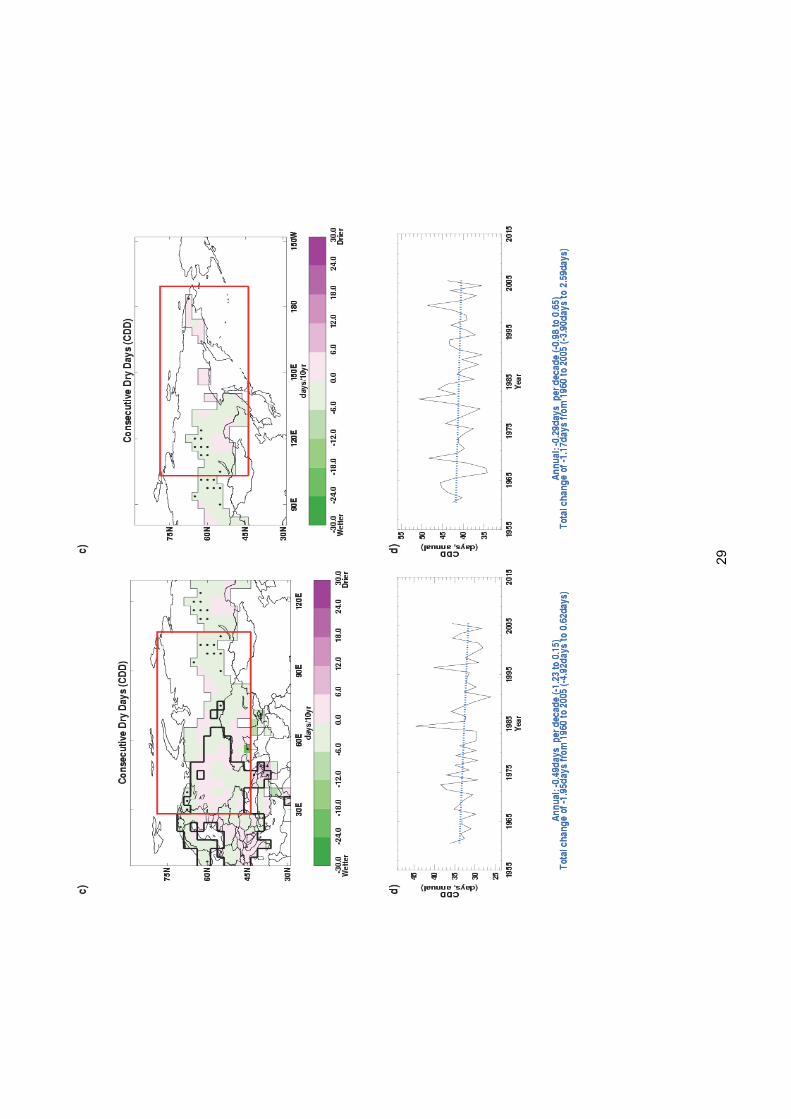
Between 1960 and 2003, over western Russia there has been a widespread increase in
annual total precipitation. Confidence is higher in this change for some grid boxes than
others, and also when regionally averaged (Figure 6). This is consistent with previous
research that found increasing precipitation between 1978 and 2005 (UNFCCC, 2010)
although with some seasonal differences. The signal shown here is more mixed for dry spell
length and especially wet spell length where data-coverage is sparser. There are spatially
consistent regions of both increasing and decreasing dry spell lengths but with low
confidence that these trends are different from zero throughout. Over eastern Russia there
have been spatially consistent increases and decreases in annual total precipitation although
confidence is lower for the vast majority of grid boxes and when regionally averaged (Figure
6b). There is very poor coverage for wet spell length, but there is a more coherent signal,
albeit weak, for dry spell length. Increasing dry spell length concurs with decreasing annual
precipitation over the easternmost regions. Conversely, decreasing dry spell length concurs

27
with increasing annual precipitation further west – there is higher confidence in these signals
for a number of grid boxes.

28
29

30
Figu
re 6
. Th
e ch
ange
in th
e an
nual
tota
l rai
nfal
l (a,
b), t
he a
nnua
l num
ber o
f con
tinuo
us d
ry d
ays
(c,d
) and
the
annu
al n
umbe
r of c
ontin
uous
wet
day
s (e
,f) o
ver t
he p
erio
d 19
60-2
010.
The
map
s an
d tim
e se
ries
have
bee
n cr
eate
d in
exa
ctly
the
sam
e w
ay a
s Fi
gure
3.
Onl
y an
nual
regi
onal
ave
rage
s ar
e sh
ow in
b,d
,f).
Hig
her c
onfid
ence
in th
e tre
nd, a
s de
fined
abo
ve u
sing
the
5th a
nd 9
th p
erce
ntile
s, is
sho
wn
as a
sol
id li
ne in
b,d
,f), l
ower
con
fiden
ce is
sho
wn
with
a d
otte
d lin
e.

31
Summary
The main features seen in observed climate over Russia from this analysis are:
x There has been widespread warming over Russia since 1960.
x Since 1960 there have been widespread increases in the frequency of warm days
and nights and decreases in the frequency of cool days and nights.
x Model results indicate a general increase in seasonal temperatures averaged over
the country as a result of human influence on climate, making the occurrence of
warm seasonal temperatures more frequent and cold seasonal temperatures less
frequent.
x Between 1960 and 2003, over western Russia there has been a widespread increase
in annual total precipitation.

32
Methodology annex
Recent, notable extremes
In order to identify what is meant by ‘recent’ events the authors have used the period since
1994, when WMO Status of the Global Climate statements were available to the authors.
However, where possible, the most notable events during the last 10 years have been
chosen as these are most widely reported in the media, remain closest to the forefront of the
memory of the country affected, and provide an example likely to be most relevant to today’s
society. By ‘notable’ the authors mean any event which has had significant impact either in
terms of cost to the economy, loss of life, or displacement and long term impact on the
population. In most cases the events of largest impact on the population have been chosen,
however this is not always the case.
Tables of recent, notable extreme events have been provided for each country. These have
been compiled using data from the World Meteorological Organisation (WMO) Annual
Statements on the Status of the Global Climate. This is a yearly report which includes
contributions from all the member countries, and therefore represents a global overview of
events that have had importance on a national scale. The report does not claim to capture all
events of significance, and consistency across the years of records available is variable.
However, this database provides a concise yet broad account of extreme events per country.
This data is then supplemented with accounts from the monthly National Oceanic and
Atmospheric Administration (NOAA) State of the Climate reports which outline global
extreme events of meteorological significance.
We give detailed examples of heat, precipitation and storm extremes for each country where
these have had significant impact. Where a country is primarily affected by precipitation or
heat extremes this is where our focus has remained. An account of the impact on human life,
property and the economy has been given, based largely on media reporting of events, and
official reports from aid agencies, governments and meteorological organisations. Some
data has also been acquired from the Centre for Research on Epidemiological Disasters
(CRED) database on global extreme events. Although media reports are unlikely to be
completely accurate, they do give an indication as to the perceived impact of an extreme
event, and so are useful in highlighting the events which remain in the national psyche.
Our search for data has not been exhaustive given the number of countries and events
included. Although there are a wide variety of sources available, for many events, an official

33
account is not available. Therefore figures given are illustrative of the magnitude of impact
only (references are included for further information on sources). It is also apparent that the
reporting of extreme events varies widely by region, and we have, where possible, engaged
with local scientists to better understand the impact of such events.
The aim of the narrative for each country is to provide a picture of the social and economic
vulnerability to the current climate. Examples given may illustrate the impact that any given
extreme event may have and the recovery of a country from such an event. This will be
important when considering the current trends in climate extremes, and also when
examining projected trends in climate over the next century.
Observational record
In this section we outline the data sources which were incorporated into the analysis, the
quality control procedure used, and the choices made in the data presentation. As this report
is global in scope, including 23 countries, it is important to maintain consistency of
methodological approach across the board. For this reason, although detailed datasets of
extreme temperatures, precipitation and storm events exist for various countries, it was not
possible to obtain and incorporate such a varied mix of data within the timeframe of this
project. Attempts were made to obtain regional daily temperature and precipitation data from
known contacts within various countries with which to update existing global extremes
databases. No analysis of changes in storminess is included as there is no robust historical
analysis of global land surface winds or storminess currently available.
Analysis of seasonal mean temperature
Mean temperatures analysed are obtained from the CRUTEM3 global land-based surface-
temperature data-product (Brohan et al. 2006), jointly created by the Met Office Hadley
Centre and Climatic Research Unit at the University of East Anglia. CRUTEM3 comprises of
more than 4000 weather station records from around the world. These have been averaged
together to create 5° by 5° gridded fields with no interpolation over grid boxes that do not
contain stations. Seasonal averages were calculated for each grid box for the 1960 to 2010
period and linear trends fitted using the median of pairwise slopes (Sen 1968; Lanzante
1996). This method finds the slopes for all possible pairs of points in the data, and takes
their median. This is a robust estimator of the slope which is not sensitive to outlying points.
High confidence is assigned to any trend value for which the 5th to 95th percentiles of the
pairwise slopes are of the same sign as the trend value and thus inconsistent with a zero
trend.

34
Analysis of temperature and precipitation extremes using indices
In order to study extremes of climate a number of indices have been created to highlight
different aspects of severe weather. The set of indices used are those from the World
Climate Research Programme (WCRP) Climate Variability and Predictability (CLIVAR)
Expert Team on Climate Change Detection and Indices (ETCCDI). These 27 indices use
daily rainfall and maximum and minimum temperature data to find the annual (and for a
subset of the indices, monthly) values for, e.g., the ‘warm’ days where daily maximum
temperature exceeds the 90th percentile maximum temperature as defined over a 1961 to
1990 base period. For a full list of the indices we refer to the website of the ETCCDI
(http://cccma.seos.uvic.ca/ETCCDI/index.shtml).
Index Description Shortname Notes
Cool night frequency
Daily minimum temperatures lower than the 10th percentile daily minimum temperature using the base reference
period 1961-1990
TN10p ---
Warm night frequency
Daily minimum temperatures higher than the 90th
percentile daily minimum temperature using the base reference period 1961-1990
TN90p ---
Cool day frequency
Daily maximum temperatures lower than the 10th percentile daily maximum temperature
using the base reference period 1961-1990
TX10p ---
Warm day frequency
Daily maximum temperatures higher than the 90th
percentile daily maximum temperature using the base reference period 1961-1990
TX90p ---
Dry spell duration Maximum duration of
continuous days within a year with rainfall <1mm
CDD
Lower data coverage due to the requirement for a
‘dry spell’ to be at least 6 days long resulting in intermittent temporal
coverage
Wet spell duration
Maximum duration of continuous days with
rainfall >1mm for a given year
CWD
Lower data coverage due to the requirement for a
‘wet spell’ to be at least 6 days long resulting in intermittent temporal
coverage Total annual precipitation Total rainfall per year PRCPTOT ---
Table 3. Description of ETCCDI indices used in this document.
A previous global study of the change in these indices, containing data from 1951-2003 can
be found in Alexander et al. 2006, (HadEX; see http://www.metoffice.gov.uk/hadobs/hadex/).

35
In this work we aimed to update this analysis to the present day where possible, using the
most recently available data. A subset of the indices is used here because they are most
easily related to extreme climate events (Table 3).
Use of HadEX for analysis of extremes
The HadEX dataset comprises all 27 ETCCDI indices calculated from station data and then
smoothed and gridded onto a 2.5° x 3.75° grid, chosen to match the output from the Hadley
Centre suite of climate models. To update the dataset to the present day, indices are
calculated from the individual station data using the RClimDex/FClimDex software;
developed and maintained on behalf of the ETCCDI by the Climate Research Branch of the
Meteorological Service of Canada. Given the timeframe of this project it was not possible to
obtain sufficient station data to create updated HadEX indices to present day for a number of
countries: Brazil; Egypt; Indonesia; Japan (precipitation only); South Africa; Saudi Arabia;
Peru; Turkey; and Kenya. Indices from the original HadEX data-product are used here to
show changes in extremes of temperature and precipitation from 1960 to 2003. In some
cases the data end prior to 2003. Table 4 summarises the data used for each country.
Below, we give a short summary of the methods used to create the HadEX dataset (for a full
description see Alexander et al. 2006).
To account for the uneven spatial coverage when creating the HadEX dataset, the indices
for each station were gridded, and a land-sea mask from the HadCM3 model applied. The
interpolation method used in the gridding process uses a decorrelation length scale (DLS) to
determine which stations can influence the value of a given grid box. This DLS is calculated
from the e-folding distance of the individual station correlations. The DLS is calculated
separately for five latitude bands, and then linearly interpolated between the bands. There is
a noticeable difference in spatial coverage between the indices due to these differences in
decorrelation length scales. This means that there will be some grid-box data where in fact
there are no stations underlying it. Here we apply black borders to grid-boxes where at least
3 stations are present to denote greater confidence in representation of the wider grid-box
area there. The land-sea mask enables the dataset to be used directly for model comparison
with output from HadCM3. It does mean, however, that some coastal regions and islands
over which one may expect to find a grid-box are in fact empty because they have been
treated as sea
36
Data sources used for updates to the HadEX analysis of extremes
We use a number of different data sources to provide sufficient coverage to update as many
countries as possible to present day. These are summarised in Table 4. In building the new
datasets we have tried to use exactly the same methodology as was used to create the
original HadEX to retain consistency with a product that was created through substantial
international effort and widely used, but there are some differences, which are described in
the next section.
Wherever new data have been used, the geographical distributions of the trends were
compared to those obtained from HadEX, using the same grid size, time span and fitting
method. If the pattern of the trends in the temperature or precipitation indices did not match
that from HadEX, we used the HadEX data despite its generally shorter time span.
Differences in the patterns of the trends in the indices can arise because the individual
stations used to create the gridded results are different from those in HadEX, and the quality
control procedures used are also very likely to be different. Countries where we decided to
use HadEX data despite the existence of more recent data are Egypt and Turkey.
GHCND:
The Global Historical Climate Network Daily data has near-global coverage. However, to
ensure consistency with the HadEX database, the GHCND stations were compared to those
stations in HadEX. We selected those stations which are within 1500m of the stations used
in the HadEX database and have a high correlation with the HadEX stations. We only took
the precipitation data if its r>0.9 and the temperature data if one of its r-values >0.9. In
addition, we required at least 5 years of data beyond 2000. These daily data were then
converted to the indices using the fclimdex software
ECA&D and SACA&D:
The European Climate Assessment and Dataset and the Southeast Asian Climate
Assessment and Dataset data are pre-calculated indices comprising the core 27 indices
from the ETCCDI as well as some extra ones. We kindly acknowledge the help of Albert
Klein Tank, the KNMI1 and the BMKG2 for their assistance in obtaining these data.
1 Koninklijk Nederlands Meteorologisch Instituut – The Royal Netherlands Meteorological Institute
2 Badan Meteorologi, Klimatologi dan Geofisika – The Indonesian Meteorological, Climatological and Geophysical Agency

37
Mexico:
The station data from Mexico has been kindly supplied by the SMN3 and Jorge Vazquez.
These daily data were then converted to the required indices using the Fclimdex software.
There are a total of 5298 Mexican stations in the database. In order to select those which
have sufficiently long data records and are likely to be the most reliable ones we performed
a cross correlation between all stations. We selected those which had at least 20 years of
data post 1960 and have a correlation with at least one other station with an r-value >0.95.
This resulted in 237 stations being selected for further processing and analysis.
Indian Gridded:
The India Meteorological Department provided daily gridded data (precipitation 1951-2007,
temperature 1969-2009) on a 1° x 1° grid. These are the only gridded daily data in our
analysis. In order to process these in as similar a way as possible the values for each grid
were assumed to be analogous to a station located at the centre of the grid. We keep these
data separate from the rest of the study, which is particularly important when calculating the
decorrelation length scale, which is on the whole larger for these gridded data.
3 Servicio Meteorológico Nacional de México – The Mexican National Meteorological Service

38
Cou
ntry
Reg
ion
box
(r
ed d
ashe
d
boxe
s in
Fig
. 1
and
on e
ach
map
at
beg
inni
ng o
f ch
apte
r)
Dat
a so
urce
(T
=
tem
pera
ture
, P
=
prec
ipita
tion)
Perio
d of
dat
a co
vera
ge
(T =
te
mpe
ratu
re, P
=
prec
ipita
tion)
Indi
ces
incl
uded
(s
ee T
able
3 fo
r de
tails
)
Tem
pora
l re
solu
tion
avai
labl
e N
otes
Arg
entin
a 73
.125
to 5
4.37
5 o W
, 21
.25
to 5
6.25
o S
Mat
ilde
Rus
ticuc
ci (T
,P)
1960
-201
0 (T
,P)
TN10
p, T
N90
p,
TX10
p, T
X90p
, P
RC
PTO
T, C
DD
, C
WD
annu
al
Aus
tralia
11
4.37
5 to
155
.625
o E
, 11.
25 to
43.
75 o S
G
HC
ND
(T,P
) 19
60-2
010
(T,P
)
TN10
p, T
N90
p,
TX10
p, T
X90p
, P
RC
PTO
T, C
DD
, C
WD
mon
thly
, se
ason
al a
nd
annu
al
Land
-sea
mas
k ha
s be
en a
dapt
ed to
incl
ude
Tasm
ania
and
the
area
aro
und
Bris
bane
Bang
lade
sh
88.1
25 to
91.
875
o E,
21.2
5 to
26.
25 o N
In
dian
Grid
ded
data
(T,P
) 19
60-2
007
(P),
1970
-200
9 (T
)
TN10
p, T
N90
p,
TX10
p, T
X90p
, P
RC
PTO
T, C
DD
, C
WD
mon
thly
, se
ason
al a
nd
annu
al
Inte
rpol
ated
from
Indi
an G
ridde
d da
ta
Bra
zil
73.1
25 to
31.
875
o W,
6.25
o N to
33.
75 o S
H
adE
X (T
,P)
1960
-200
0 (P
) 20
02 (T
)
TN10
p, T
N90
p,
TX10
p, T
X90p
, P
RC
PTO
T, C
DD
, C
WD
annu
al
Spat
ial c
over
age
is p
oor
Chi
na
73.1
25 to
133
.125
o E
, 21.
25 to
53.
75 o N
G
HC
ND
(T,P
) 19
60-1
997
(P)
1960
-200
3 (T
min)
1960
-201
0 (T
max
)
TN10
p, T
N90
p,
TX10
p, T
X90p
, P
RC
PTO
T, C
DD
, C
WD
mon
thly
, se
ason
al a
nd
annu
al
Prec
ipita
tion
has
very
poo
r cov
erag
e be
yond
19
97 e
xcep
t in
2003
-04,
and
no
data
at a
ll in
20
00-0
2, 2
005-
11
Egy
pt
24.3
75 to
35.
625
o E,
21.2
5 to
31.
25 o N
H
adE
X (T
,P)
No
data
TN
10p,
TN
90p,
TX
10p,
TX9
0p,
PR
CP
TOT,
an
nual
Th
ere
are
no d
ata
for E
gypt
so
all g
rid-b
ox
valu
es h
ave
been
inte
rpol
ated
from
sta
tions
in
Jor
dan,
Isra
el, L
ibya
and
Sud
an

39
Fran
ce
5.62
5 o W
to 9
.375
o E
, 41.
25 to
51.
25 o N
EC
A&D
(T,P
) 19
60-2
010
(T,P
)
TN10
p, T
N90
p,
TX10
p, T
X90p
, P
RC
PTO
T, C
DD
, C
WD
mon
thly
, se
ason
al a
nd
annu
al
Ger
man
y 5.
625
to 1
6.87
5 o E
, 46
.25
to 5
6.25
o N
ECA&
D (T
,P)
1960
-201
0 (T
,P)
TN10
p, T
N90
p,
TX10
p, T
X90p
, P
RC
PTO
T, C
DD
, C
WD
mon
thly
, se
ason
al a
nd
annu
al
Indi
a 69
.375
to 9
9.37
5 o E
, 6.
25 to
36.
25 o N
In
dian
Grid
ded
data
(T,P
) 19
60-2
003
(P),
1970
-200
9 (T
)
TN10
p, T
N90
p,
TX10
p, T
X90p
, P
RC
PTO
T, C
DD
, C
WD
mon
thly
, se
ason
al a
nd
annu
al
Indo
nesi
a 95
.625
to 1
40.6
25 o
E, 6
.25
o N to
11.
25 o
S
Had
EX
(T,P
) 19
68-2
003
(T,P
) TN
10p,
TN
90p,
TX
10p,
TX9
0p,
PR
CP
TOT,
an
nual
Sp
atia
l cov
erag
e is
poo
r
Italy
5.
625
to 1
6.87
5 o E
, 36
.25
to 4
6.25
o N
ECA&
D (T
,P)
1960
-201
0 (T
,P)
TN10
p, T
N90
p,
TX10
p, T
X90p
, P
RC
PTO
T, C
DD
, C
WD
mon
thly
, se
ason
al a
nd
annu
al
Land
-sea
mas
k ha
s be
en a
dapt
ed to
im
prov
e co
vera
ge o
f Ita
ly
Japa
n 12
9.37
5 to
144
.375
o E
, 31.
25 to
46.
25 o N
H
adE
X (P
) G
HC
ND
(T)
1960
-200
3 (P
) 19
60-2
000
(Tm
in)
1960
-201
0 (T
max
)
TN10
p, T
N90
p,
TX10
p, T
X90p
, P
RC
PTO
T,
mon
thly
, se
ason
al a
nd
annu
al (T
), an
nual
(P)
Ken
ya
31.8
75 to
43.
125
o E,
6.25
o N to
6.2
5 o S
H
adE
X (T
,P)
1960
-199
9 (P
) TN
10p,
TN
90p,
TX
10p,
TX9
0p,
PR
CP
TOT
an
nual
Ther
e ar
e no
tem
pera
ture
dat
a fo
r Ken
ya
and
so g
rid-b
ox v
alue
s ha
ve b
een
inte
rpol
ated
from
nei
ghbo
urin
g U
gand
a an
d th
e U
nite
d R
epub
lic o
f Tan
zani
a. R
egio
nal
aver
ages
incl
ude
grid
-box
es fr
om o
utsi
de
Ken
ya th
at e
nabl
e co
ntin
uatio
n to
200
3
Mex
ico
118.
125
to 8
8.12
5 o
W, 1
3.75
to 3
3.75
o N
Raw
sta
tion
data
fro
m th
e S
ervi
cio
Met
eoro
lógi
co
Nac
iona
l (S
MN
) (T
,P)
1960
-200
9 (T
,P)
TN10
p, T
N90
p,
TX10
p, T
X90p
, P
RC
PTO
T, C
DD
, C
WD
mon
thly
, se
ason
al a
nd
annu
al
237/
5298
sta
tions
sel
ecte
d. N
on u
nifo
rm
spat
ial c
over
age.
Dro
p in
T a
nd P
cov
erag
e in
200
9.
40
Per
u 84
.735
to 6
5.62
5 o W
, 1.
25 o
N t
o 18
.75
o S
Had
EX
(T,P
) 19
60-2
002
(T,P
)
TN10
p, T
N90
p,
TX10
p, T
X90p
, P
RC
PTO
T, C
DD
, C
WD
annu
al
Inte
rmitt
ent c
over
age
in T
X90p
, CD
D a
nd
CW
D
Rus
sia
Wes
t Rus
sia
28
.125
to 1
06.8
75 o
E, 4
3.75
to 7
8.75
o N,
Eas
t Rus
sia
10
3.12
5 to
189
.375
o E
, 43.
75 to
78.
75 o N
ECA&
D (T
,P)
1960
-201
0 (T
,P)
TN10
p, T
N90
p,
TX10
p, T
X90p
, P
RC
PTO
T, C
DD
, C
WD
mon
thly
, se
ason
al a
nd
annu
al
Cou
ntry
spl
it fo
r pre
sent
atio
n pu
rpos
es o
nly.
Saud
i Ara
bia
31.8
75 to
54.
375
o E,
16.2
5 to
33.
75 o N
H
adE
X (T
,P)
1960
-200
0 (T
,P)
TN10
p, T
N90
p,
TX10
p, T
X90p
, P
RC
PTO
T an
nual
Sp
atia
l cov
erag
e is
poo
r
Sou
th A
frica
13
.125
to 3
5.62
5 o W
, 21
.25
to 3
6.25
o S
Had
EX
(T,P
) 19
60-2
000
(T,P
)
TN10
p, T
N90
p,
TX10
p, T
X90p
, P
RC
PTO
T, C
DD
, C
WD
annu
al
---
Rep
ublic
of
Kor
ea
125.
625
to 1
29.3
75 o
E, 3
3.75
to 3
8.75
o N
Had
EX
(T,P
) 19
60-2
003
(T,P
) TN
10p,
TN
90p,
TX
10p,
TX9
0p,
PR
CP
TOT,
CD
D
annu
al
Ther
e ar
e to
o fe
w d
ata
poin
ts fo
r CW
D to
ca
lcul
ate
trend
s or
regi
onal
tim
eser
ies
Spai
n 9.
375
o W to
1.8
75 o
E, 3
6.25
to 4
3.75
o N
ECA&
D (T
,P)
1960
-201
0 (T
,P)
TN10
p, T
N90
p,
TX10
p, T
X90p
, P
RC
PTO
T, C
DD
, C
WD
mon
thly
, se
ason
al a
nd
annu
al
Turk
ey
24.3
75 to
46.
875
o E,
36.2
5 to
43.
75 o N
H
adE
X (T
,P)
1960
-200
3 (T
,P)
TN10
p, T
N90
p,
TX10
p, T
X90p
, P
RC
PTO
T, C
DD
, C
WD
annu
al
Inte
rmitt
ent c
over
age
in C
WD
and
CD
D w
ith
no re
gion
al a
vera
ge b
eyon
d 20
00
Uni
ted
King
dom
9.
375
o W to
1.8
75 o
E, 5
1.25
to 5
8.75
o N
ECA&
D (T
,P)
1960
-201
0 (T
,P)
TN10
p, T
N90
p,
TX10
p, T
X90p
, P
RC
PTO
T, C
DD
, C
WD
mon
thly
, se
ason
al a
nd
annu
al
Uni
ted
Sta
tes
of A
mer
ica
125.
625
to 6
5.62
5 o
W, 2
3.75
to 4
8.75
o N
GH
CN
D (T
,P)
1960
-201
0 (T
,P)
TN10
p, T
N90
p,
TX10
p, T
X90p
, P
RC
PTO
T, C
DD
, C
WD
mon
thly
, se
ason
al a
nd
annu
al
Tabl
e 4.
Sum
mar
y of
dat
a us
ed fo
r eac
h co
untry
.

41
Quality control and gridding procedure used for updates to the HadEX analysis of extremes
In order to perform some basic quality control checks on the index data, we used a two-step
process on the indices. Firstly, internal checks were carried out, to remove cases where the
5 day rainfall value is less than the 1 day rainfall value, the minimum T_min is greater than
the minimum T_max and the maximum T_min is greater than the maximum T_max.
Although these are physically impossible, they could arise from transcription errors when
creating the daily dataset, for example, a misplaced minus sign, an extra digit appearing in
the record or a column transposition during digitisation. During these tests we also require
that there are at least 20 years of data in the period of record for the index for that station,
and that some data is found in each decade between 1961 and 1990, to allow a reasonable
estimation of the climatology over that period.
Weather conditions are often similar over many tens of kilometres and the indices calculated
in this work are even more coherent. The correlation coefficient between each station-pair
combination in all the data obtained is calculated for each index (and month where
appropriate), and plotted as a function of the separation. An exponential decay curve is fitted
to the data, and the distance at which this curve has fallen by a factor 1/e is taken as the
decorrelation length scale (DLS). A DLS is calculated for each dataset separately. For the
GHCND, a separate DLS is calculated for each hemisphere. We do not force the fitted
decay curve to show perfect correlation at zero distance, which is different to the method
employed when creating HadEX. For some of the indices in some countries, no clear decay
pattern was observed in some data sets or the decay was so slow that no value for the DLS
could be determined. In these cases a default value of 200km was used.
We then perform external checks on the index data by comparing the value for each station
with that of its neighbours. As the station values are correlated, it is therefore likely that if
one station measures a high value for an index for a given month, its neighbours will also be
measuring high. We exploit this coherence to find further bad values or stations as follows.
Although raw precipitation data shows a high degree of localisation, using indices which have
monthly or annual resolution improves the coherence across wider areas and so this
neighbour checking technique is a valid method of finding anomalous stations.
We calculate a climatology for each station (and month if appropriate) using the mean value
for each index over the period 1961-1990. The values for each station are then anomalised
using this climatology by subtracting this mean value from the true values, so that it is clear if
the station values are higher or lower than normal. This means that we do not need to take

42
differences in elevation or topography into account when comparing neighbours, as we are
not comparing actual values, but rather deviations from the mean value.
All stations which are within the DLS distance are investigated and their anomalised values
noted. We then calculate the weighted median value from these stations to take into account
the decay in the correlation with increasing distance. We use the median to reduce the
sensitivity to outliers.
If the station value is greater than 7.5 median-absolute-deviations away from the weighted
median value (this corresponds to about 5 standard deviations if the distribution is Gaussian,
but is a robust measure of the spread of the distribution), then there is low confidence in the
veracity of this value and so it is removed from the data.
To present the data, the individual stations are gridded on a 3.75o x 2.5o grid, matching the
output from HadCM3. To determine the value of each grid box, the DLS is used to calculate
which stations can reasonably contribute to the value. The value of each station is then
weighted using the DLS to obtain a final grid box value. At least three stations need to have
valid data and be near enough (within 1 DLS of the gridbox centre) to contribute in order for a
value to be calculated for the grid point. As for the original HadEX, the HadCM3 land-sea
mask is used. However, in three cases the mask has been adjusted as there are data over
Tasmania, eastern Australia and Italy that would not be included otherwise (Figure 7).
Figure 7. Land Sea mask used for gridding the station data and regional areas allocated to each country as described in Table 2.
43
Presentation of extremes of temperature and precipitation
Indices are displayed as regional gridded maps of decadal trends and regional average time-
series with decadal trends where appropriate. Trends are fitted using the median of pairwise
slopes method (Sen 1968, Lanzante 1996). Trends are considered to be significantly
different from a zero trend if the 5th to 95th percentiles of the pairwise slopes do not
encompass zero. This is shown by a black dot in the centre of the grid-box or by a solid line
on time-series plots. This infers that there is high confidence in the sign (positive or negative)
of the sign. Confidence in the trend magnitude can be inferred by the spread of the 5th to 95th
percentiles of the pairwise slopes which is given for the regional average decadal trends.
Trends are only calculated when there are data present for at least 50% of years in the
period of record and for the updated data (not HadEX) there must be at least one year in
each decade.
Due to the practice of data-interpolation during the gridding stage (using the DLS) there are
values for some grid boxes when no actually station lies within the grid box. There is more
confidence in grid boxes for which there are underlying data. For this reason, we identify
those grid boxes which contain at least 3 stations by a black contour line on the maps. The
DLS differs with region, season and index which leads to large differences in the spatial
coverage. The indices, by their nature of being largely threshold driven, can be intermittent
over time which also affects spatial and temporal coverage (see Table 3).
Each index (and each month for the indices for which there is monthly data) has a different
DLS, and so the coverage between different indices and datasets can be different. The
restrictions on having at least 20 years of data present for each input station, at least 50% of
years in the period of record and at least one year in each decade for the trending calculation,
combined with the DLS, can restrict the coverage to only those regions with a dense station
network reporting reliably.
Each country has a rectangular region assigned as shown by the red dashed box on the map
in Figure 7 and listed in Table 4, which is used for the creation of the regional average. This
is sometimes identical to the attribution region shown in grey on the map in Figure 7. This
region is again shown on the maps accompanying the time series of the regional averages
as a reminder of the region and grid boxes used in the calculation. Regional averages are
created by weighting grid box values by the cosine of their grid box centre latitude. To ensure
consistency over time a regional average is only calculated when there are a sufficient
number of grid boxes present. The full-period median number of grid-boxes present is
calculated. For regions with a median of more than six grid-boxes there must be at least 80%

44
of the median number of grid boxes present for any one year to calculate a regional average.
For regions with six or fewer median grid boxes this is relaxed to 50%. These limitations
ensure that a single station or grid box which has a longer period of record than its
neighbours cannot skew the timeseries trend. So sometimes there may be grid-boxes
present but no regional average time series. The trends for the regional averages are
calculated in the same way as for the individual grid boxes, using the median of pairwise
slopes method (Sen 1968, Lanzante 1996). Confidence in the trend is also determined if the
5th to 95th percentiles of the pairwise slopes are of the same sign and thus inconsistent with a
zero trend. As well as the trend in quantity per decade, we also show the full change in the
quantity from 1960 to 2010 that this fitted linear trend implies.

45
Fi
gure
8.
Exa
mpl
es o
f the
plo
ts s
how
n in
the
data
sec
tion.
Lef
t: Fr
om E
CA
&D
dat
a be
twee
n 19
60-2
010
for t
he n
umbe
r of w
arm
nig
hts,
and
Rig
ht: f
rom
H
adE
X d
ata
(196
0-20
03) f
or th
e to
tal p
reci
pita
tion.
A fu
ll ex
plan
atio
n of
the
plot
s is
giv
en in
the
text
bel
ow.

46
The results are presented in the form of a map and a time series for each country and index.
The map shows the grid box decadal trend in the index over the period for which there are
data. High confidence, as determined above, is shown by a black dot in the grid box centre.
To show the variation over time, the values for each year (and month if available) are shown
in a time series for a regional average. The values of the indices have been normalised to a
base period of 1961-1990 (except the Indian gridded data which use a 1971 to 1990 period),
both in HadEX and in the new data acquired for this project. Therefore, for example, the
percentage of nights exceeding the 90th percentile for a temperature is 10% for that period.
There are two influences on whether a grid box contains a value or not – the land-sea mask,
and the decorrelation length scale. The land-sea mask is shown in Figure 7. There are grid
boxes which contain some land but are mostly sea and so are not considered. The
decorrelation length scale sets the maximum distance a grid box can be from stations before
no value is assigned to it. Grid boxes containing three or more stations are highlighted by a
thick border. This indicates regions where the value shown is likely to be more representative
of the grid box area mean as opposed to a single station location.
On the maps for the new data there is a box indicating which grid boxes have been extracted
to calculate the area average for the time series. This box is the same as shown in Figure 7
at the beginning of each country’s document. These selected grid boxes are combined using
area (cosine) weighting to calculate the regional average (both annual [thick lines] and
monthly [thin lines] where available). Monthly (orange) and annual (blue) trends are fitted to
these time series using the method described above. The decadal trend and total change
over the period where there are data are shown with 5th to 95th percentile confidence
intervals in parentheses. High confidence, as determined above, is shown by a solid line as
opposed to a dotted one. The green vertical lines on the time series show the dates of some
of the notable events outlined in each section.
Attribution
Regional distributions of seasonal mean temperatures in the 2000s are computed with and
without the effect of anthropogenic influences on the climate. The analysis considers
temperatures averaged over the regions shown in Figure 3. These are also identified as grey
boxes on the maps in Figure 7. The coordinates of the regions are given in Table 5. The
methodology combines information from observations and model simulations using the
approach originally introduced in Christidis et al., 2010 and later extended in Christidis et al.,

47
2011, where more details can be found. The analysis requires spatial scales greater than
about 2,500 km and for that reason the selected regions (Fig.9 and Table 5) are often larger
than individual countries, or include several smaller countries in a single region (for example
UK, Germany and France are grouped in one region).
Observations of land temperature come from the CRUTEM3 gridded dataset (Brohan et al.,
2006) and model simulations from two coupled GCMs, namely the Hadley Centre HadGEM1
model (Martin et al., 2006) and version 3.2 of the MIROC model (K-1 Developers, 2004). The
use of two GCMs helps investigate the sensitivity of the results to the model used in the
analysis. Ensembles of model simulations from two types of experiments are used to
partition the temperature response to external forcings between its anthropogenic and
natural components. The first experiment (ALL) simulates the combined effect of natural and
anthropogenic forcings on the climate system and the second (ANTHRO) includes
anthropogenic forcings only. The difference of the two gives an estimate of the effect of the
natural forcings (NAT). Estimates of the effect of internal climate variability are derived from
long control simulations of the unforced climate. Distributions of the regional summer mean
temperature are computed as follows:
a) A global optimal fingerprinting analysis (Allen and Tett, 1999; Allen and Stott, 2003) is
first carried out that scales the global simulated patterns (fingerprints) of climate
change attributed to different combinations of external forcings to best match them to
the observations. The uncertainty in the scaling that originates from internal variability
leads to samples of the scaled fingerprints, i.e. several realisations that are plausibly
consistent with the observations. The 2000-2009 decade is then extracted from the
scaled patterns and two samples of the decadal mean temperature averaged over the
reference region are then computed with and without human influences, which
provide the Probability Density Functions (PDFs) of the decadal mean temperature
attributable to ALL and NAT forcings.
b) Model-derived estimates of noise are added to the distributions to take into account
the uncertainty in the simulated fingerprints.
c) In the same way, additional noise from control model simulations is introduced to the
distributions to represent the effect of internal variability in the annual values of the
seasonal mean temperatures. The result is a pair of estimated distributions of the
annual values of the seasonal mean temperature in the region with and without the
effect of human activity on the climate. The temperatures throughout the analysis are
expressed as anomalies relative to period 1961-1990.
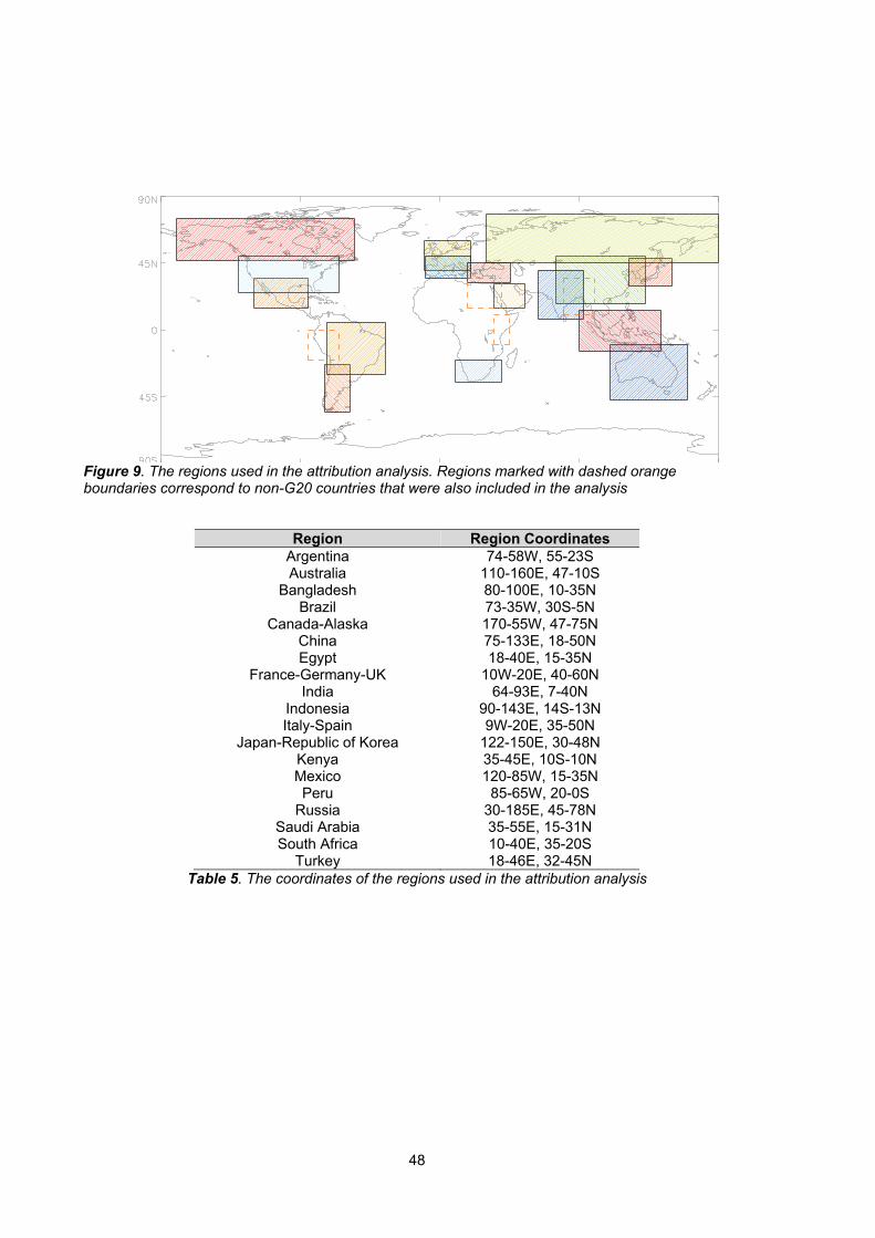
48
Figure 9. The regions used in the attribution analysis. Regions marked with dashed orange boundaries correspond to non-G20 countries that were also included in the analysis
Region Region Coordinates
Argentina Australia
Bangladesh Brazil
Canada-Alaska China Egypt
France-Germany-UK India
Indonesia Italy-Spain
Japan-Republic of Korea Kenya Mexico Peru
Russia Saudi Arabia South Africa
Turkey
74-58W, 55-23S 110-160E, 47-10S 80-100E, 10-35N 73-35W, 30S-5N 170-55W, 47-75N 75-133E, 18-50N 18-40E, 15-35N
10W-20E, 40-60N 64-93E, 7-40N
90-143E, 14S-13N 9W-20E, 35-50N
122-150E, 30-48N 35-45E, 10S-10N 120-85W, 15-35N
85-65W, 20-0S 30-185E, 45-78N 35-55E, 15-31N 10-40E, 35-20S 18-46E, 32-45N
Table 5. The coordinates of the regions used in the attribution analysis

49
References
ALEXANDER, L. V., ZHANG. X., PETERSON, T. C., CAESAR, J., GLEASON, B., KLEIN
TANK, A. M. G., HAYLOCK, M., COLLINS, D., TREWIN, B., RAHIMZADEH, F., TAGIPOUR,
A., RUPA KUMAR, K., REVADEKAR, J., GRIFFITHS, G., VINCENT, L., STEPHENSON, D.
B., BURN, J., AGUILAR, E., BRUNET, M., TAYLOR, M., NEW, M., ZHAI, P., RUSTICUCCI,
M. and VAZQUEZ-AGUIRRE, J. L. 2006. Global observed changes in daily climate extremes
of temperature and precipitation. J. Geophys. Res. 111, D05109. doi:10.1029/2005JD006290.
ALLEN, M. R., TETT S. F. B. 1999. Checking for model consistency in optimal fingerprinting.
Clim Dyn 15: 419-434
ALLEN M. R., STOTT P. A. 2003. Estimating signal amplitudes in optimal fingerprinting, part
I: theory. Clim Dyn 21: 477-491
BROHAN, P., KENNEDY, J.J., HARRIS, I., TETT, S.F.B. and JONES, P.D. 2006.
Uncertainty estimates in regional and global observed temperature changes: a new dataset
from 1850. J. Geophys. Res. 111, D12106. doi:10.1029/2005JD006548.
BULYGINA, O., N. N. KORSHUNOVA, AND V. N. RAZUVAEV. 2003. Regional Climates
Asia, Russia, in State of the Climate in 2002. Bulletin of the American Meteorological Society
S48–S50.
BULYGINA, O. 2004. Regional Climate Asia, Russia, in State of the Climate in 2003. Bulletin
of the American Meteorological Society S55–S57.
BULYGINA, O. N., N. N. KORSHUNOVA, and V. N. RAZUVAEV. 2006. Regional Climates
Asia, Russia, in State of the Climate in 2005. Bulletin of the American Meteorological Society
S71-S73.
BULYGINA, O. N., N. N. KORSHUNOVA, and V. N. RAZUVAEV. 2007. Regional Climates
Asia, west and central Asia, in State of the Climate in 2006. Bulletin of the American
Meteorological Society S94-S97.
BULYGINA, O. N., N. N. KORSHUNOVA, and V. N. RAZUVAEV. 2008. Regional Climates
Asia, Russia, in State of the Climate in 2007. Bulletin of the American Meteorological Society
89 (7), S131-S133.

50
BULYGINA, O. N., N. N. KORSHUNOVA, and N. RAZUVAEV. 2009. Regional Climates Asia,
Russia, in State of the Climate in 2008. Bulletin of the American Meteorological Society 90
(8), S153-S155.
BULYGINA, O. N., N. N. KORSHUNOVA, and N. RAZUVAEV. 2010. Regional Climates Asia,
Russia, in State of the Climate in 2009. Bulletin of the American Meteorological Society 91
(7), S170-S174.
CHRISTIDIS N., STOTT. P A., ZWIERS, F. W., SHIOGAMA, H., NOZAWA, T. 2010.
Probabilistic estimates of recent changes in temperature: a multi-scale attribution analysis.
Clim Dyn 34: 1139-1156
CHRISTIDIS, N., STOTT, P. A., ZWIERS, F. W., SHIOGAMA, H., NOZAWA, T. 2011. The
contribution of anthropogenic forcings to regional changes in temperature during the last
decade. Climate Dynamics in press.
DURRE, I, MENNE, MJ, GLEASON, BE, HOUSTON, TG, VOSE, RS, 2010. Comprehensive
Automated Quality Assurance of Daily Surface Observations, Journal of Applied Meteorology
and Climatology, 49, 8, 1615-1633
K-1 MODEL DEVELOPERS (2004) K-1 coupled GCM (MIROC) description, K-1 Tech Rep,
H Hasumi and S Emori (eds), Centre for Clim Sys Res, Univ of Tokyo
KLEIN TANK, A.M.G. et al. 2002. Daily dataset of 20th-century surface air temperature and
precipitation series for the European Climate Assessment. Int. J. of Clim. 22, 1441-1453.
LANZANTE, J. R. 1996. Resistant, robust and non-parametric techniques for the analysis of
climate data: theory and examples, including applications to historical radiosonde station
data. Int. J. Clim. 16, 1197–226.
MAIER, F., A. OBREGÓN, P. BISSOLLI, C. ACHBERGER , J. J. KENNEDY, D. E. PARKER ,
O. BULYGINA, and N. KORSHUNOVA. 2011. Summer heat waves in Eastern Europe and
western Russia in State of the Climate in 2010. Bulletin of the American Meteorological
Society 92, S210.
MARTIN G.M., RINGER. M. A., POPE V. D., JONES, A., DEARDEN, C., HINTON, T. 2006.
The physical properties of the atmosphere in the new Hadley Centre Global Environmental
Model (HadGEM1). Part I: Model description and global climatology. J Clim 19: 1274-1301

51
SANCHEZ-LUGO, A., KENNEDY, J.J. and BERRISFORD, P. 2011. Global Climate, Surface
Temperatures in State of the Climate 2010. Bulletin of the American Meteorological Society
92 (6), S36-S37.
SEN, P. K. 1968. Estimates of the regression coefficient based on Kendall’s tau. J. Am. Stat.
Assoc. 63, 1379–89.
UNFCCC – ɉəɌɈȿ ɇȺɐɂɈɇȺɅɖɇɈȿ ɋɈɈȻɓȿɇɂȿ ɊɈɋɋɂɃɋɄɈɃ ɎȿȾȿɊȺɐɂɂ –
Ɇɨɫɤɜɚ 2010 ɝ. – Fifth national communication by the government of the Russian Federation
to the United Nations Framework Convention on Climate Change – Russian Federation
http://unfccc.int/resource/docs/natc/rus_nc5_resubmit.pdf direct translation – DdG 27 June
2011.
WAPLE, A. M., J. H. LAWRIMORE, M. S. HALPERT, G. D. BELL, W. HIGGINS, B. LYON, M.
J. MENNE, K. L. GLEASON, R. C. SCHNELL, J. R. CHRISTY, W. THIAW, W. J. WRIGHT, M.
J. SALINGER, L. ALEXANDER, R. S. STONE, and S. J. CAMARGO. 2002. Regional
Climate Asia, Harsh Siberian Winter, in Climate Assessment for 2001. Bulletin of the
American Meteorological Society S49–S50.
WMO WORLD METEOROLOGICAL ORGANIZATION. 2001. Statement on Status of the
Global Climate in 2000, WMO-No. 920.
http://www.wmo.int/pages/prog/wcp/wcdmp/statement/wmostatement_en.html
WMO WORLD METEOROLOGICAL ORGANIZATION. 2002. Statement on Status of the
Global Climate in 2001, WMO-No. 940.
http://www.wmo.int/pages/prog/wcp/wcdmp/statement/wmostatement_en.html
WMO WORLD METEOROLOGICAL ORGANIZATION. 2003. Statement on Status of the
Global Climate in 2002, WMO-No. 949.
http://www.wmo.int/pages/prog/wcp/wcdmp/statement/wmostatement_en.html
WMO WORLD METEOROLOGICAL ORGANIZATION. 2004. Statement on Status of the
Global Climate in 2003, WMO-No. 966.
http://www.wmo.int/pages/prog/wcp/wcdmp/statement/wmostatement_en.html
WMO WORLD METEOROLOGICAL ORGANIZATION. 2005. Statement on Status of the
Global Climate in 2004, WMO-No. 983.
http://www.wmo.int/pages/prog/wcp/wcdmp/statement/wmostatement_en.html

52
WMO WORLD METEOROLOGICAL ORGANIZATION. 2006. Statement on Status of the
Global Climate in 2005, WMO-No. 998.
http://www.wmo.int/pages/prog/wcp/wcdmp/statement/wmostatement_en.html
WMO WORLD METEOROLOGICAL ORGANIZATION. 2007. Statement on Status of the
Global Climate in 2006, WMO-No. 1016.
http://www.wmo.int/pages/prog/wcp/wcdmp/statement/wmostatement_en.html
WMO WORLD METEOROLOGICAL ORGANIZATION. 2008. Statement on Status of the
Global Climate in 2007, WMO-No. 1031.
http://www.wmo.int/pages/prog/wcp/wcdmp/statement/wmostatement_en.html
WMO WORLD METEOROLOGICAL ORGANIZATION. 2009. Statement on Status of the
Global Climate in 2008, WMO-No. 1039.
http://www.wmo.int/pages/prog/wcp/wcdmp/statement/wmostatement_en.html
WMO WORLD METEOROLOGICAL ORGANIZATION. 2011. Statement on Status of the
Global Climate in 2010, WMO-No. 1074.
http://www.wmo.int/pages/prog/wcp/wcdmp/statement/wmostatement_en.html

53
Acknowledgements
Data for this work were taken from the GHCND database (Durre et al. 2010). We thank Lisa
Alexander and Markus Donat (University of New South Wales) for their help and advice.

54

55
�
�
�
Chapter 2 – Climate Change Projections
�

56
Introduction
Climate models are used to understand how the climate will evolve over time and typically
represent the atmosphere, ocean, land surface, cryosphere, and biogeochemical processes,
and solve the equations governing their evolution on a geographical grid covering the globe.
Some processes are represented explicitly within climate models, large-scale circulations for
instance, while others are represented by simplified parameterisations. The use of these
parameterisations is sometimes due to processes taking place on scales smaller than the
typical grid size of a climate model (a Global Climate Model (GCM) has a typical horizontal
resolution of between 250 and 600km) or sometimes to the current limited understanding of
these processes. Different climate modelling institutions use different plausible
representations of the climate system, which is why climate projections for a single
greenhouse gas emissions scenario differ between modelling institutes. This gives rise to
“climate model structural uncertainty”.
In response to a proposed activity of the World Climate Research Programme's (WCRP's;
http://www.wcrp-climate.org/) Working Group on Coupled Modelling (WGCM), the Program
for Climate Model Diagnosis and Intercomparison (PCMDI; http://www-pcmdi.llnl.gov/)
volunteered to collect model output contributed by leading climate modelling centres around
the world. Climate model output from simulations of the past, present and future climate was
collected by PCMDI mostly during the years 2005 and 2006, and this archived data
constitutes phase 3 of the Coupled Model Intercomparison Project (CMIP3). In part, the
WGCM organised this activity to enable those outside the major modelling centres to
perform research of relevance to climate scientists preparing the IPCC Fourth Assessment
Report (AR4). This unprecedented collection of recent model output is commonly known as
the “CMIP3 multi-model dataset". The GCMs included in this dataset are referred to
regularly throughout this review, although not exclusively.
The CMIP3 multi-model ensemble has been widely used in studies of regional climate
change and associated impacts. Each of the constituent models was subject to extensive
testing by the contributing institute, and the ensemble has the advantage of having been
constructed from a large pool of alternative model components, therefore sampling
alternative structural assumptions in how best to represent the physical climate system.
Being assembled on an opportunity basis, however, the CMIP3 ensemble was not designed
to represent model uncertainties in a systematic manner, so it does not, in isolation, support

57
robust estimates of the risk of different levels of future climate change, especially at a
regional level.
Since CMIP3, a new (CMIP5) generation of coupled ocean-atmosphere models has been
developed, which is only just beginning to be available and is being used for new projections
for the IPCC Fifth Assessment Report (AR5).
These newer models typically feature higher spatial resolution than their CMIP3 counterparts,
including in some models a more realistic representation of stratosphere-troposphere
interactions. The CMIP5 models also benefit from several years of development in their
parameterisations of small scale processes, which, together with resolution increases, are
expected to result in a general improvement in the accuracy of their simulations of historical
climate, and in the credibility of their projections of future changes. The CMIP5 programme
also includes a number of comprehensive Earth System Models (ESMs) which explicitly
simulate the earth's carbon cycle and key aspects of atmospheric chemistry, and also
contain more sophisticated representations of aerosols compared to CMIP3 models.
The CMIP3 results should be interpreted as a useful interim set of plausible outcomes.
However, their neglect of uncertainties, for instance in carbon cycle feedbacks, implies that
higher levels of warming outside the CMIP3 envelope cannot be ruled out. In future, CMIP5
coupled model and ESM projections can be expected to produce improved advice on future
regional changes. In particular, ensembles of ESM projections will be needed to provide a
more comprehensive survey of possible future changes and their relative likelihoods of
occurrence. This is likely to require analysis of the CMIP5 multi-model ESM projections,
augmented by larger ensembles of ESM simulations in which uncertainties in physical and
biogeochemical feedback processes can be explored more systematically, for example via
ensembles of model runs in which key aspects of the climate model are slightly adjusted.
Note that such an exercise might lead to the specification of wider rather than narrower
uncertainties compared to CMIP3 results, if the effects of representing a wider range of earth
system processes outweigh the effects of refinements in the simulation of physical
atmosphere-ocean processes already included in the CMIP3 models.

58
Climate projections
The Met Office Hadley Centre is currently producing perturbed parameter ensembles of a
single model configuration known as HadCM3C, to explore uncertainties in physical and
biogeochemical feedback processes. The results of this analysis will become available in the
next year and will supplement the CMIP5 multi-model ESM projections, providing a more
comprehensive set of data to help progress understanding of future climate change.
However, many of the studies covered in the chapter on climate impacts have used CMIP3
model output. For this reason, and because it is still the most widely used set of projections
available, the CMIP3 ensemble output for temperature and precipitation, for the A1B
emission scenario, for Russia and the surrounding region is shown below.
���� �Figure 1. Percentage change in average annual temperature by 2100 from 1960-1990 baseline climate, averaged over 21 CMIP3 models. The size of each pixel represents the level of agreement between models on the magnitude of the change.

59
����� �Figure 2. Percentage change in average annual precipitation by 2100 from 1960-1990 baseline climate, averaged over 21 CMIP3 models. The size of each pixel represents the level of agreement between models on the sign of the change.
Summary of temperature change in Russia
Figure 1 shows the percentage change in average annual temperature by 2100 from 1960-
1990 baseline climate, averaged over 21 CMIP3 models. All of the models in the CMIP3
ensemble project increased temperatures in the future, but the size of each pixel indicates
how well the models agree over the magnitude of the increase.
Projected changes in temperature are higher over northern parts of the country, with
increases of above 5.5°C in the Arctic regions. In central parts of the country, increases
range between around 4.5-5.5°C, and in southern and western regions, increases lie in the
range of 3.5-4°C. There is moderate agreement between the models over most of Russia.
Summary of precipitation change in Russia
Figure 2 shows the percentage change in average annual precipitation by 2100 from 1960-
1990 baseline climate, averaged over 21 CMIP3 models. Unlike for temperature, the models
sometimes disagree over whether precipitation is increasing or decreasing over a region, so
in this case the size of each pixel indicates the percentage of the models in the ensemble
that agree on the sign of the change in precipitation.
Precipitation is projected to increase over almost the entire country. Increases of above
20% are projected in the north of the country, with most other regions projected to
experience increases of between 10% and 20%. In the Caucasus region, projected

60
precipitation change ranges from an increase of 5% to a decrease of 5%. Ensemble
agreement over the changes is high over most of the country, but more moderate in parts of
the southwest.

61
Chapter 3 – Climate Change Impact Projections

62
Introduction
Aims and approach
This chapter looks at research on a range of projected climate change impacts, with focus
on results for Russia. It includes projections taken from the AVOID programme, for some of
the impact sectors.
The aim of this work is to take a ‘top down’ approach to assessing global impacts studies,
both from the literature and from new research undertaken by the AVOID programme. This
project covers 23 countries, with summaries from global studies provided for each of these.
This global approach allows some level of comparison between countries, whilst presenting
information on a scale most meaningful to inform international policy.
The literature covered in this chapter focuses on research published since the Fourth
Assessment Report (AR4) of the Intergovernmental Panel on Climate Change (IPCC) and
should be read in conjunction with IPCC AR4 WG1 and WG2 reports. For some sectors
considered, an absence of research developments since the IPCC AR4, means earlier work
is cited as this helps describe the current level of scientific understanding. This report
focuses on assessing scientific research about climate change impacts within sectors; it
does not present an integrated analysis of climate change adaptation policies.
Some national and sub-national scale literature is reported to a limited extent to provide
some regional context.
Impact sectors considered and methods
This report reviews the evidence for the impact of climate change on a number of sectors,
for Russia. The following sectors are considered in turn in this report:
x Crop yields
x Food security
x Water stress and drought
x Pluvial flooding and rainfall
x Fluvial flooding
x Tropical cyclones (where applicable)

63
x Coastal regions
Supporting literature
Literature searches were conducted for each sector with the Thomson Reuters Web of
Science (WoS., 2011) and Google Scholar academic search engines respectively.
Furthermore, climate change impact experts from each of the 23 countries reviewed were
contacted. These experts were selected through a combination of government nomination
and from experts known to the Met Office. They were asked to provide literature that they
felt would be of relevance to this review. Where appropriate, such evidence has been
included. A wide range of evidence was considered, including; research from international
peer-reviewed journal papers; reports from governments, non-governmental organisations,
and private businesses (e.g. reinsurance companies), and research papers published in
national journals.
For each impact sector, results from assessments that include a global- or regional-scale
perspective are considered separately from research that has been conducted at the
national- or sub-national-scale. The consideration of global- and regional-scale studies
facilitates a comparison of impacts across different countries, because such studies apply a
consistent methodology for each country. While results from national- and sub-national-scale
studies are not easily comparable between countries, they can provide a level of detail that
is not always possible with larger-scale studies. However, the national- and sub-national
scale literature included in this project does not represent a comprehensive coverage of
regional-based research and cannot, and should not, replace individual, detailed impacts
studies in countries. The review aims to present an up-to-date assessment of the impact of
climate change on each of the sectors considered.
AVOID programme results
Much of the work in this report is drawn from modelling results and analyses coming out of
the AVOID programme. The AVOID programme is a research consortium funded by DECC
and Defra and led by the UK Met Office and also comprises the Walker Institute at the
University of Reading, the Tyndall Centre represented through the University of East Anglia,
and the Grantham Institute for Climate Change at Imperial College. The expertise in the
AVOID programme includes climate change research and modelling, climate change
impacts in natural and human systems, socio-economic sciences, mitigation and technology.

64
The unique expertise of the programme is in bringing these research areas together to
produce integrated and policy-relevant results. The experts who work within the programme
were also well suited to review the literature assessment part of this report. In this report the
modelling of sea level rise impacts was carried out for the AVOID programme by the
University of Southampton.
The AVOID programme uses the same emissions scenarios across the different impact
sectors studied. These are a business as usual (IPCC SRES A1B) and an aggressive
mitigation (the AVOID A1B-2016-5-L) scenario. Model output for both scenarios was taken
from more than 20 GCMs and averaged for use in the impact models. The impact models
are sector specific, and frequently employ further analytical techniques such as pattern
scaling and downscaling in the crop yield models.
Data and analysis from AVOID programme research is provided for the following impact
sectors:
x Crop yields
x Water stress and drought
x Fluvial flooding
x Coastal regions
Uncertainty in climate change impact assessment
There are many uncertainties in future projections of climate change and its impacts. Several
of these are well-recognised, but some are not. One category of uncertainty arises because
we don’t yet know how mankind will alter the climate in the future. For instance, uncertainties
in future greenhouse gas emissions depends on the future socio-economic pathway, which,
in turn, depends on factors such as population, economic growth, technology development,
energy demand and methods of supply, and land use. The usual approach to dealing with
this is to consider a range of possible future scenarios.
Another category of uncertainties relate to our incomplete understanding of the climate
system, or an inability to adequately model some aspects of the system. This includes:
x Uncertainties in translating emissions of greenhouse gases into atmospheric
concentrations and radiative forcing. Atmospheric CO2 concentrations are currently
rising at approximately 50% of the rate of anthropogenic emissions, with the
remaining 50% being offset by a net uptake of CO2 into the oceans and land

65
biosphere. However, this rate of uptake itself probably depends on climate, and
evidence suggests it may weaken under a warming climate, causing more CO2 to
remain in the atmosphere, warming climate further. The extent of this feedback is
highly uncertain, but it not considered in most studies. The phase 3 of the Coupled
Model Intercomparison Project (CMIP3), which provided the future climate
projections for the IPCC Fourth Assessment Report (AR4), used a single estimate of
CO2 concentration rise for each emissions scenario, so the CMIP3 projections (which
were used in most studies presented here, including AVOID) do not account for this
uncertainty.
x Uncertainty in climate response to the forcing by greenhouse gases and aerosols.
One aspect of this is the response of global mean temperature (“climate sensitivity”),
but a more relevant aspect for impacts studies is the response of regional climates,
including temperature, precipitation and other meteorological variables. Different
climate models can give very different results in some regions, while giving similar
results in other regions. Confidence in regional projections requires more than just
agreement between models: physical understanding of the relevant atmospheric,
ocean and land surface processes is also important, to establish whether the models
are likely to be realistic.
x Additional forcings of regional climate. Greenhouse gas changes are not the only
anthropogenic driver of climate change; atmospheric aerosols and land cover change
are also important, and unlike greenhouse gases, the strength of their influence
varies significantly from place to place. The CMIP3 models used in most impacts
studies generally account for aerosols but not land cover change.
x Uncertainty in impacts processes. The consequences of a given changes in weather
or climatic conditions for biophysical impacts such as river flows, drought, flooding,
crop yield or ecosystem distribution and functioning depend on many other
processes which are often poorly-understood, especially at large scales. In particular,
the extent to which different biophysical impacts interact with each other has been
hardly studied, but may be crucial; for example, impacts of climate change on crop
yield may depend not only on local climate changes affecting rain-fed crops, but also
remote climate changes affecting river flows providing water for irrigation.
x Uncertainties in non-climate effects of some greenhouse gases. As well as being a
greenhouse gas, CO2 exerts physiological influences on plants, affecting
photosynthesis and transpiration. Under higher CO2 concentrations, and with no

66
other limiting factors, photosynthesis can increase, while the requirements of water
for transpiration can decrease. However, while this has been extensively studied
under experimental conditions, including in some cases in the free atmosphere, the
extent to which the ongoing rise in ambient CO2 affects crop yields and natural
vegetation functioning remains uncertain and controversial. Many impacts
projections assume CO2 physiological effects to be significant, while others assume it
to be non-existent. Studies of climate change impacts on crops and ecosystems
should therefore be examined with care to establish which assumptions have been
made.
In addition to these uncertainties, the climate varies significantly through natural processes
from year-to-year and also decade-to-decade, and this variability can be significant in
comparison to anthropogenic forcings on shorter timescales (the next few decades)
particularly at regional scales. Whilst we can characterise the natural variability it will not be
possible to give a precise forecast for a particular year decades into the future.
A further category of uncertainty in projections arises as a result of using different methods
to correct for uncertainties and limitations in climate models. Despite being painstakingly
developed in order to represent current climate as closely as possible, current climate
models are nevertheless subject to systematic errors such as simulating too little or too
much rainfall in some regions. In order to reduce the impact of these, ‘bias correction’
techniques are often employed, in which the climate model is a source of information on the
change in climate which is then applied to the observed present-day climate state (rather
than using the model’s own simulation of the present-day state). However, these bias-
corrections typically introduce their own uncertainties and errors, and can lead to
inconsistencies between the projected impacts and the driving climate change (such as river
flows changing by an amount which is not matched by the original change in precipitation).
Currently, this source of uncertainty is rarely considered
When climate change projections from climate models are applied to climate change impact
models (e.g. a global hydrological model), the climate model structural uncertainty carries
through to the impact estimates. Additional uncertainties include changes in future emissions
and population, as well as parameterisations within the impact models (this is rarely
considered). Figure 1 highlights the importance of considering climate model structural
uncertainty in climate change impacts assessment. Figure 1 shows that for 2°C prescribed
global-mean warming, the magnitude of, and sign of change in average annual runoff from
present, simulated by an impacts model, can differ depending upon the GCM that provides
the climate change projections that drive the impact model. This example also shows that

67
the choice of impact model, in this case a global hydrological model (GHM) or catchment-
scale hydrological model (CHM), can affect the magnitude of impact and sign of change from
present (e.g. see IPSL CM4 and MPI ECHAM5 simulations for the Xiangxi). To this end,
throughout this review, the number of climate models applied in each study reviewed, and
the other sources of uncertainty (e.g. emissions scenarios) are noted. Very few studies
consider the application of multiple impacts models and it is recommended that future
studies address this.
�Figure 1. Change in average annual runoff relative to present (vertical axis; %), when a global hydrological model (GHM) and a catchment-scale hydrological model (CHM) are driven with climate change projections from 7 GCMs (horizontal axis), under a 2°C prescribed global-mean warming scenario, for six river catchments. The figure is from Gosling et al. (2011). �
A key uncertainty in climate projections for Russia includes the extent of the Arctic sea ice
retreat. Following a record minima in 2007, Arctic summer sea ice extent recovered back to
the long-term trend line in 2009 (Fetterer et al., 2009), although estimates of thickness
suggest that it is significantly thinner as a result of being largely composed of thin first year
ice. It has been argued that the decline in 2007 was not particularly unusual in the context of
the observational record (Notz, 2009), especially given that variability might be expected to
increase as the sea ice thins (Goosse et al., 2009, Notz, 2009). However, abrupt reductions
in future Arctic summer sea ice extent are seen in projections from several GCMs included in
the CMIP3 multi-model dataset (Holland et al., 2006). Although there remains uncertainty, it
is still considered likely that sea ice decline could be reversible (Notz, 2009), although some
consequences of a temporary, but complete, seasonal loss of sea ice (e.g. for biodiversity)
might be irreversible.
Methods combining observational constraints with model projections suggest that summer
sea ice may disappear earlier than simulated by many (but not all) CMIP3 multi-model
dataset models reported in the IPCC AR4, probably before the end of the century under a
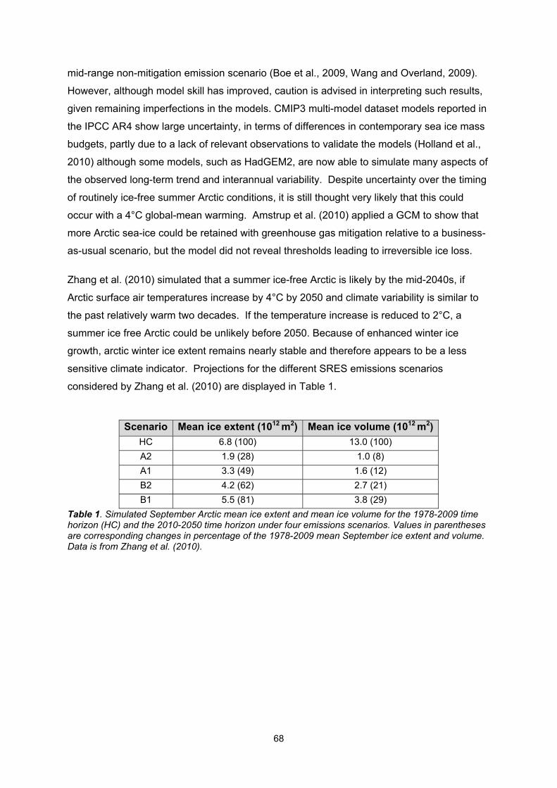
68
mid-range non-mitigation emission scenario (Boe et al., 2009, Wang and Overland, 2009).
However, although model skill has improved, caution is advised in interpreting such results,
given remaining imperfections in the models. CMIP3 multi-model dataset models reported in
the IPCC AR4 show large uncertainty, in terms of differences in contemporary sea ice mass
budgets, partly due to a lack of relevant observations to validate the models (Holland et al.,
2010) although some models, such as HadGEM2, are now able to simulate many aspects of
the observed long-term trend and interannual variability. Despite uncertainty over the timing
of routinely ice-free summer Arctic conditions, it is still thought very likely that this could
occur with a 4°C global-mean warming. Amstrup et al. (2010) applied a GCM to show that
more Arctic sea-ice could be retained with greenhouse gas mitigation relative to a business-
as-usual scenario, but the model did not reveal thresholds leading to irreversible ice loss.
Zhang et al. (2010) simulated that a summer ice-free Arctic is likely by the mid-2040s, if
Arctic surface air temperatures increase by 4°C by 2050 and climate variability is similar to
the past relatively warm two decades. If the temperature increase is reduced to 2°C, a
summer ice free Arctic could be unlikely before 2050. Because of enhanced winter ice
growth, arctic winter ice extent remains nearly stable and therefore appears to be a less
sensitive climate indicator. Projections for the different SRES emissions scenarios
considered by Zhang et al. (2010) are displayed in Table 1.
Scenario Mean ice extent (1012 m2) Mean ice volume (1012 m2)
HC 6.8 (100) 13.0 (100) A2 1.9 (28) 1.0 (8) A1 3.3 (49) 1.6 (12) B2 4.2 (62) 2.7 (21) B1 5.5 (81) 3.8 (29)
Table 1. Simulated September Arctic mean ice extent and mean ice volume for the 1978-2009 time horizon (HC) and the 2010-2050 time horizon under four emissions scenarios. Values in parentheses are corresponding changes in percentage of the 1978-2009 mean September ice extent and volume. Data is from Zhang et al. (2010).�
69
Summary of findings for each sector
Crop yields
x Quantitative crop yield projections under climate change scenarios for Russia vary
greatly across studies due to the application of different models, assumptions and
emissions scenarios.
x Whilst a definitive conclusion on the impact of climate change on crop yields in
Russia cannot be drawn, the majority of global- and regional-scale studies included
in this report project a decrease in the yield of wheat, Russia’s major crop, as a
consequence of climate change.
x Studies from the AVOID programme suggest a mixed outcome, with some areas of
cultivated land becoming more suitable for agriculture, and other areas becoming
less suitable, as a result of climate change.
x Important knowledge gaps and key uncertainties include the quantification of yield
increases due to CO2 fertilisation, the quantification of yield reductions due to ozone
damage and the extent to which crop diseases might affect crop yields with climate
change.
Food security
x Russia is currently a country with extremely low levels of undernourishment. The
majority of global- and regional-scale studies included here project that although
negatively affected, the country is unlikely to face severe food security issues over
the next 40 years as a consequence of climate change.
x National-scale assessments are consistent in showing that climate change could
have a negative impact on food security in Russia.
x One study concluded that Russia’s economy could present a high vulnerability to the
impact of climate change on fisheries by the 2050s. Another projected that the 10-
year averaged maximum catch potential from 2005 to 2055 could see around a 20%
increase under the A1B emission scenario.

70
Water stress and drought
x Global-scale studies included here show that the west of Russia is the most
vulnerable region of the country to water stress. For the rest of the country and
particularly the east, vulnerability is presently low.
x A number of global-scale studies included here project an increase in water
availability across Russia as a whole with climate change, although there is regional
variation, with an increase in water stress possible for the west of the country.
x However, recent simulations from the AVOID programme show consensus across
models for little change in the population exposed to increased or decreased water
stress with climate change.
Pluvial flooding and rainfall
x Recent studies suggest that winter precipitation could increase for Russia under
climate change, and there is consistency across different climate models in this
change.
x There is less agreement across climate models for precipitation changes in summer,
however.
x Increases in precipitation from extreme storm events are also possible with climate
change, although such projections cannot be translated directly into flood projections
without detailed local-scale impact models, incorporating topography and hydrology.
Fluvial flooding
x Recent studies have suggested that flood magnitudes for Central and Eastern
Siberia and the Russian Far East may increase with climate change, but decrease in
European Russia and West Siberia, due to smaller maximum rates of snowmelt
runoff.
x Results from simulations by the AVOID programme, that applied climate change
projections from 21 climate models, show a high level of agreement among models
that flood risk for Russia as a whole could decrease with climate change throughout
the 21st century.

71
x Although most studies present a useful indicator of exposure to flood risk with climate
change, none of them account for the effect that hydropower reservoirs, present in
most large rivers, can have on the height of the annual flood peak, which can be
substantial. Also, few studies have investigated the occurrence of ice dams and the
potential resultant flooding with climate change.
Tropical cyclones
x Russia is not impacted by tropical cyclones.
Coastal regions
x There is very little work on the impact of climate change on Russia’s coastal regions.
x However one study estimates that the population exposure to sea level rise (SLR)
could increase from 189,000 in present to 226,000 under un-mitigated A1B
emissions in 2070. Relative to A1B an aggressive mitigation policy could avoid an
exposure of around 28,000 people by 2070. The study estimated that population
exposure to sea level rise (SLR) could increase from 189,000 in present to 226,000
under un-mitigated A1B emissions in 2070; an aggressive mitigation scenario could
avoid an exposure of around 28,000 people, relative to un-mitigated climate change
in 2070.
x Nevertheless, further studies on the impact of climate change on Russia’s coastal
regions could improve understanding.

72
Crop yields
Headline
Crop yield projections under climate change scenarios for Russia vary greatly across studies
due to the application of different models, assumptions and emissions scenarios. The
majority of studies focus on wheat and potatoes but the wide range in impact estimates
precludes a robust conclusion on the impact of climate change on crop yields in Russia.
Results from the AVOID programme for Russia indicate that the balance of impacts is more
towards increasing rather than decreasing suitability in 2030 in both scenarios. However, as
the 21st century progresses, the balance shifts more towards decreasing suitability, with this
shift being small under the mitigation scenario but larger under A1B, partly because of
smaller areas showing increasing suitability but mainly because larger areas undergo
declining suitability.
Supporting literature
Introduction
The impacts of climate change on crop productivity are highly uncertain due to the
complexity of the processes involved. Most current studies are limited in their ability to
capture the uncertainty in regional climate projections, and often omit potentially important
aspects such as extreme events and changes in pests and diseases. Importantly, there is a
lack of clarity on how climate change impacts on drought are best quantified from an
agricultural perspective, with different metrics giving very different impressions of future risk.
The dependence of some regional agriculture on remote rainfall, snowmelt and glaciers adds
to the complexity - these factors are rarely taken into account, and most studies focus solely
on the impacts of local climate change on rain-fed agriculture. However, irrigated agricultural
land produces approximately 40-45 % of the world’s food (Doll and Siebert 2002), and the
water for irrigation is often extracted from rivers which can depend on climatic conditions far
from the point of extraction. Hence, impacts of climate change on crop productivity often
need to take account of remote as well as local climate changes. Indirect impacts via sea-
level rise, storms and diseases have also not been quantified. Perhaps most seriously, there
is high uncertainty in the extent to which the direct effects of CO2 rise on plant physiology will
interact with climate change in affecting productivity. Therefore, at present, the aggregate
impacts of climate change on large-scale agricultural productivity cannot be reliably

73
quantified (Gornall et al, 2010). This section summarises findings from a range of post IPCC
AR4 assessments to inform and contextualise the analysis performed by AVOID programme
for this project. The results from the AVOID work are discussed in the next section.
Wheat, sugar beet, potatoes and cereals (maize, barley, oats and rye) are Russia’s most
important crops (see Table 2) (FAO, 2008).
Harvested area (ha) Quantity (Metric ton) Value ($1000) Wheat 26000000 Wheat 63700000 Wheat 6670000 Barley 9420000 Sugar beet 28900000 Potatoes 2820000
Sunflower seed 5980000 Potatoes 28800000 Sunflower seed 1540000 Oats 3400000 Barley 23100000 Sugar beet 1310000 Rye 2130000 Sunflower seed 7350000 Tomatoes 459000
Potatoes 2100000 Maize 6680000 Apples 421000 Maize 1730000 Oats 5830000 Vegetables fresh (nes) 1 416000
1 nes = not elsewhere specified or included Table 2. The top 7 crops by harvested area, quantity and value according to the FAO (2008) in Russia. Crops that feature in all lists are shaded green; crops that feature in two top 7 lists are shaded amber. Data is from FAO (2008) and has been rounded down to three significant figures.
A number of global impact model studies looking at crop yield which include results for some
of the main crops in Russia have been conducted. They apply a variety of methodological
approaches, including using different climate model inputs and treatment of other factors that
might affect yield, such as impact of increased CO2 in the atmosphere on plant growth and
adaption of agricultural practises to changing climate conditions. These different models,
assumptions and emissions scenarios mean that there are a range of crop yield projections
for Russia.
Important knowledge gaps and key uncertainties which are applicable to Russia as well as at
the global scale, include: the quantification of yield increases due to CO2 fertilisation and
yield reductions due to ozone damage (Ainsworth and McGrath, 2010, Iglesias et al., 2009),
and the extent crop diseases could affect crop yields with climate change (Luck et al., 2011).
Most crop simulation models do not include the direct effect of extreme temperatures on
crop development and growth, thus only changes in mean climate conditions are considered
to affect crop yields for the studies included here.
Assessments that include a global or regional perspective
Recent Past Crop yield changes could be due to a variety of factors, which might include, but not be
confined to, a changing climate. In order to assess the impact of recent climate change

74
(1980-2008) on wheat, maize, rice and soybean, Lobell et al. (2011) looked at how the
overall yield trend in these crops changed in response to changes in climate over the period
studied. The study was conducted at the global-scale but national estimates for Russia were
also calculated. Lobell et all. (2011) divided the climate-induced yield trend by the overall
yield trend for 1980–2008, to produce a simple metric of the importance of climate relative to
all other factors. The ratio produced indicates the influence of climate on the productivity
trend. So for example a value of –0.1 represents a 10% reduction in yield gain due to
climate change, compared to the increase that could have been achieved without climate
change, but with technology and other gains. This can also be expressed as 10 years of
climate trend being equivalent to the loss of roughly 1 year of technology gains. For Russia,
maize, soybean and wheat yield were impacted adversely, relative to what would have been
achieved without the climate trends (see Table 3).
Crop TrendMaize -0.2 to -0.1 Rice 0.0 to 0.1
Wheat -0.3 to -0.2 Soybean -0.2 to -0.1
Table 3. The estimated net impact of climate trends for 1980-2008 on crop yields in Russia. Climate-induced yield trend divided by overall yield trend. Data is from Lobell et al. (2011). �
Climate change studies
Several recent studies have applied climate projections from Global Climate Models (GCMs)
to crop models to assess the global-scale impact of climate change on crop yields (Iglesias
and Rosenzweig, 2009, Tatsumi et al., 2011, Fischer, 2009). Most of these studies include
impact estimates at the national-scale for Russia, which are presented in this section. The
process of CO2 fertilisation of some crops is usually included in most climate impact studies
of yields. However, other gases can influence crop yield and are not always included in
impacts models. An example of this is ozone (O3) and so a study which attempts to quantify
the potential impact on crop yield of changes in ozone in the atmosphere is also included
(Avnery et al. 2011). In addition to these studies, the AVOID programme analysed the
patterns of climate change for 21 GCMs, to establish an index of ‘climate suitability’ of
agricultural land. Climate suitability is not directly equivalent to crop yields, but is a means of
looking at a standard metric across all the countries including in this project, and of
assessing the level of agreement on variables that affect crop production, between all 21
GCMs.
Iglesias and Rosenzweig (2009) repeated an earlier study presented by Parry et al. (2004)
by applying climate projections from the HadCM3 GCM (instead of HadCM2, which was

75
applied by Parry et al. (2004)), under seven SRES emissions scenarios and for three future
time periods. This study used a globally consistent crop simulation methodologies and
climate change scenarios, and weighted the model site results by their contribution to
regional and national, and rain-fed and irrigated production. The study also applied a
quantitative estimation of physiological CO2 effects on crop yields and considered the effect
of adaptation by assessing the country or regional potential for reaching optimal crop yield.
The results from the study for Russia are presented in Table 4 and Table 5. The simulations
showed that relative to the baseline (1970-2000) yield levels, crop yield losses were
projected for each of the crops with climate change for all time horizons. Under all emissions
scenarios (except A1FI) and B1a, wheat yield was estimated to increase between 2050 and
2080; the declining yield trend for maize on the other hand was not reversed.
Scenario Year Wheat Maize
A1FI
2020 -3.19 -6.19 2050 -4.56 -11.56 2080 -5.07 -15.07
A2a
2020 -3.16 -6.16 2050 -3.38 -10.38 2080 -0.41 -11.41
A2b
2020 -2.89 -5.89 2050 -4.37 -11.37 2080 -2.70 -13.70
A2c
2020 -1.89 -4.89 2050 -3.92 -10.92 2080 -1.04 -12.04
B1a
2020 -5.57 -8.57 2050 -3.29 -8.29 2080 -5.82 -11.82
B2a
2020 -5.85 -8.85 2050 -4.33 -9.33 2080 -2.99 -9.99
B2b
2020 -4.09 -7.09 2050 -7.48 -12.48 2080 -4.71 -11.71
Table 4. Wheat and maize yield changes (%) in Russia relative to baseline scenario (1970-2000) for different emission scenarios and future time periods. Some emissions scenarios were run in an ensemble simulation (e.g. A2a, A2b, A2c). Data is from Iglesias and Rosenzweig (2009).

76
Wheat Maize
Up Down Up DownBaseline to 2020 0 7 0 7 Baseline to 2050 0 7 0 7 Baseline to 2080 0 7 0 7 2020 to 2050 2 5 1 6 2050 to 2080 5 2 1 6
Table 5. The number of emission scenarios that predict yield gains (“Up”) or yield losses (“Down”) for wheat and maize in Russia between two points in time. Data is from Iglesias and Rosenzweig (2009).�
Tatsumi et al. (2011) applied an improved version of the GAEZ crop model (iGAEZ) to
simulate crop yields on a global scale for wheat, potato, cassava, soybean, rice, sweet
potato, maize, green beans. The impact of global warming on crop yields from the 1990s to
2090s was assessed by projecting five GCM outputs under the SRES A1B scenario and
comparing the results for crop yields as calculated using the iGAEZ model for the period of
1990-1999. The results for Russia are displayed in Table 6 and suggest a general decline in
yields of all crops modelled, except for rice.
Wheat Potato Cassava Soybean Rice Sweet
potato Maize Green
beans
-8.28 -9.24 - -10.73 11.45 - -11.5 -
Table 6. Average change in yield (%), during 1990s-2090s in Russia. Data is from Tatsumi et al. (2011).
Fischer (2009) projected global ‘production potential’ changes for 2050 using the GAEZ
(Global Agro-Ecological Zones) crops model with climate change scenarios from the
HadCM3 and CSIRO GCMs respectively, under SRES A2 emissions. The impacts of future
climate on crop yields of rain-fed cereals in Russia (relative to yield realised under current
climate) are presented in Table 7. Contrary to the previous studies these results suggest an
increase in the crop yield potential, especially for maize and sorghum.

77
CO2 fert.
2020s 2050s 2080s
CSIRO HADCM3 CSIRO HADCM3 CSIRO HADCM3
Rain-fed wheat
Yes 4 3 4 5 -15 -1 No 1 n/a -2 n/a -23 n/a
Rain-fed maize
Yes 64 54 79 67 69 63 No 61 n/a 73 n/a 62 n/a
Rain-fed cereals
Yes n/a 5 n/a 9 n/a 6 No n/a n/a n/a n/a n/a n/a
Rain-fed sorghum
Yes 60 n/a 75 n/a 70 n/a No 57 n/a 68 n/a 62 n/a
Table 7. Impacts of climate change on the production potential in Russia of rain-fed cereals in current cultivated land (% change with respect to yield realised under current climate), with two GCMs and with and without CO2 fertilisation (“CO2 fert.”) under SRES A2 emissions. Data is from Fischer (2009).
In addition to the studies looking at the effect of changes in climate and CO2 concentrations
on crop yield, Avnery et al. (2011) investigated the effects of ozone surface exposure on
crop yield losses for soybeans, maize and wheat under the SRES A2 and B1 scenarios
respectively. Two metrics of ozone exposure were investigated; seasonal daytime (08:00-
19:59) mean O3 (“M12”) and accumulated O3 above a threshold of 40 ppbv (“AOT40”). The
effect of the ozone exposure was considered in isolation from climate and other changes.
The results for Russia are presented in Table 8.
A2 B1 M12 AOT40 M12 AOT40
Soybeans - - - - Maize 6-8 2-4 4-6 0-2 Wheat 2-4 15-20 0-2 8-10
Table 8. National relative crop yield losses (%) for 2030 under A2 and B1 emission scenarios according to the M12 (seasonal daytime (08:00–19:59) mean) and AOT40 (accumulated O3 above a threshold of 40 ppbv) metrics of O3 exposure. Data is from Avnery et al. (2011).
National-scale or sub-national scale assessments
Climate change studies
In this section we present results from recent studies that have produced national or sub-
national scale projections of future crop yields in Russia.
Alcamo et al. (2007a) assessed the impact of climate change on Russian agriculture by
applying climate projections from two GCMs under SRES A2 and B2 emissions scenarios.
The authors also accounted for the frequency (and spatial heterogeneity) of extreme climate
events. The simulations suggested that decreased crop production in some Russian regions

78
could be compensated by increased production in others, thus resulting in relatively small
average changes (see Table 9). However, the frequency of food production shortfall years (a
year in which potential production of the most important crops in a region is below 50% of its
average climate normal production) doubled in many of the main crop growing areas in the
2020s, and tripled in the 2070s.
2020 2070 A2 B2 A2 B2
Grain Potato Grain Potato Grain Potato Grain Potato ECHAM4 112 96 101 105 95 96 95 97 HadCM3 94 106 91 122 90 104 88 104
Table 9. Climate-related potential crop production (calculated from crop yield) in Russia, expressed as percentage of current mean potential crop production (average annual production from 1961 to 1990 = 100%). Grain included wheat and rye. Data is from Alcamo et al. (2007a). Dronin and Kirilenko (2008) also assessed the impact of climate change on Russian crop
production. The authors applied the same GCMs and emissions scenarios as Alcamo et al.
(2007a) and showed that crop production declined in the 2020s and 2070s from baseline
levels (see Figure 2). However, the authors did not consider the potential yield increases in
regions that currently do not produce wheat or the CO2 fertilisation effect.
Figure 2. Russian wheat production change (as a proportion of current (1961-1990) production) under HADCM3 and ECHAM4 runs (the range across GCMs is included in the errorbars), employing SRES A2 and B2 emission scenarios and the GAEZ-R crop model. Minimum, first quartile, mean, third quartile, and maximum annual yield are shown. ‘Current actual’ represents observed production as reported by the Russian National Statistics Committee (GosComStat) whereas ‘Current GCM’ represents wheat production as estimated by GAEZ-R simulations. Figure is from Dronin and Kirilenko (2008). No need to pay for copyright, if we register with RightsLink for this figure.

79
AVOID programme results
To further quantify the impact of climate change on crops, the AVOID programme simulated
the effect of climate change on the suitability of land for crop cultivation for all countries
reviewed in this literature assessment based upon the patterns of climate change from 21
GCMs (Warren et al., 2010). This ensures a consistent methodological approach across all
countries and takes consideration of climate modelling uncertainties.
Methodology
The effect of climate change on the suitability of land for crop cultivation is characterised
here by an index which defines the percentage of cropland in a region with 1) a decrease in
suitability or 2) an increase in suitability. A threshold change of 5% is applied here to
characterise decrease or increase in suitability. The crop suitability index is calculated at a
spatial resolution of 0.5°x0.5°, and is based on climate and soil properties (Ramankutty et al.,
2002). The baseline crop suitability index, against which the future changes are measured, is
representative conditions circa 2000. The key features of the climate for the crop suitability
index are temperature and the availability of water for plants, and changes in these were
derived from climate model projections of future changes in temperature and precipitation,
with some further calculations then being used to estimate actual and potential
evapotranspiration as an indicator of water availability. It should be noted that changes in
atmospheric CO2 concentrations can decrease evapotranspiration by increasing the
efficiency of water use by plants (Ramankutty et al., 2002), but that aspect of the index was
not included in the analysis here. Increased CO2 can also increase photosynthesis and
improve yield to a small extent, but again these effects are not included. Exclusion of these
effects may lead to an overestimate of decreases in suitability.
The index here is calculated only for grid cells which contain cropland circa 2000, as defined
in the global crop extent data set described by Ramankutty et al. (2008) which was derived
from satellite measurements. It is assumed that crop extent does not change over time. The
crop suitability index varies significantly for current croplands across the world (Ramankutty
et al., 2002), with the suitability being low in some current cropland areas according to this
index. Therefore, while climate change clearly has the potential to decrease suitability for
cultivation if temperature and precipitation regimes become less favourable, there is also
scope for climate change to increase suitability in some existing cropland areas if conditions
become more favourable in areas where the suitability index is not at its maximum value of 1.
It should be noted that some areas which are not currently croplands may already be
suitable for cultivation or may become suitable as a result of future climate change, and may

80
become used a croplands in the future either as part of climate change adaptation or
changes in land use arising for other reasons. Such areas are not included in this analysis.
Results
Crop suitability was estimated under the pattern of climate change from 21 GCMs with two
emissions scenarios; 1) SRES A1B and 2) an aggressive mitigation scenario where
emissions follow A1B up to 2016 but then decline at a rate of 5% per year thereafter to a low
emissions floor (denoted A1B-2016-5-L). The application of 21 GCMs is an attempt to
quantify the uncertainty due to climate modelling, although it is acknowledged that only one
crop suitability impacts model is applied. Simulations were performed for the years 2030,
2050, 2080 and 2100. The results for Russia are presented in Figure 3.
Under all the climate projections, some existing cropland areas become less suitable for
cultivation while other existing cropland areas become more suitable. The areas of
increased and decreased suitability differ considerably according to the climate model used,
and these differences between models increase into the future, especially in the A1B
scenario.
In both scenarios, between 39% and 62% of current Russian croplands become more
suitable for cultivation by 2030. In the mitigation scenario, the range of projected areas
undergoing increased suitability becomes larger through the 21st century, with the lowest
projection falling slightly to 37% while the highest projection rises to 69% - however, the
mean of all model projections remains similar over time. However, for the A1B scenario, the
difference between model projections of areas of increased suitability becomes rather larger,
ranging from 22% to 73% by 2100 with the mean projection falling from 47% in 2030 to 40%
in 2100. For both scenarios, between 3% and 43% of current Russian croplands are
projected to undergo declining suitability by 2030. By 2100 this rises to 10%-50% under the
mitigation scenario and 15%-75% under A1B.
So, for Russia, the balance of impacts is more towards increasing rather than declining
suitability in 2030 in both scenarios. However, as the 21st century progresses, the balance
shifts more towards declining suitability, with this shift being small under the mitigation
scenario but larger under A1B, partly because of smaller areas showing increasing suitability
but mainly because larger areas undergo declining suitability.

81
Figure 3. Box and whisker plots for the impact of climate change on increased crop suitability (top panel) and decreased crop suitability (bottom panel) for Russia, from 21 GCMs under two emissions scenarios (A1B and A1B-2016-5-L), for four time horizons. The plots show the 25th, 50th, and 75th percentiles (represented by the boxes), and the maximum and minimum values (shown by the extent of the whiskers).

82
Food security
Headline
There is no consensus across studies regarding the impact of climate change on food
security for Russia. A number of global-scale assessments suggest that food security may
not be an issue with climate change and that Russia might be able to export food due to
surplus. A different global-scale assessment suggests that Russia may need to limit food
exports to avoid major food insecurity under climate change, however. National-scale
assessments are consistent in showing that climate change could have a negative impact on
food security in Russia.
Supporting literature
Introduction
Food security is a concept that encompasses more than just crop production, but is a
complex interaction between food availability and socio-economic, policy and health factors
that influence access to food, utilisation and stability of food supplies. In 1996 the World
Food Summit defined food security as existing ‘when all people, at all times, have physical
and economic access to sufficient, safe and nutritious food to meet their dietary needs, and
their food preferences are met for an active and healthy life’. As such this section cannot be
a comprehensive analysis of all the factors that are important in determining food security,
but does attempt to assess a selection of the available literature on how climate change,
combined with projections of global and regional population and policy responses, may
influence food security.
With regards to food security Russia is presently a country of very low concern, relative to
other countries across the globe. According to FAO statistics (FAO, 2010) Russia has
extremely low rates of undernourishment (less than 5% of the population). However, a
number of global studies disagree about the effect of climate change on food security in
Russia in the future. These differences are in part, due to the application of different climate
models, crops models and food security models. Additional uncertainties concern the
response of capture fisheries to climate change. These uncertainties call for a
comprehensive assessment of the impact of climate change on food security in Russia.

83
Assessments that include a global or regional perspective
Several recent studies have analysed food security under climate change across the globe.
Wu et al. (2011) simulated crop yields with the GIS-based Environmental Policy Integrated
Climate (EPIC) model. This was combined with crop areas simulated by a crop choice
decision model to calculate total food production and per capita food availability across the
globe, which was used to represent the status of food availability and stability. The study
focussed on the SRES A1 scenario and applied climate change simulations for the 2000s
(1991–2000) and 2020s (2011–2020). The climate simulations were performed by MIROC
(Model for Interdisciplinary Research on Climate) version 3.2., which means the effects of
climate model uncertainty were not considered. Downscaled population and GDP data from
the International Institute for Applied Systems Analysis (IIASA) were applied in the
simulations. Wu et al. (2011) concluded that Russia is not likely to face severe food
insecurity in the next 20 years
However, the results presented by Wu et al. (2011) are in stark contrast to the results of a
study presented by Arnell et al. (2010) who demonstrated how important adaptation
measures could be for Russia, if major food security issues are to be avoided under climate
change. The study considered the impacts of global climate change and mitigation policy on
food security for eleven countries. The study applied climate change patterns from the
HadCM3 GCM and explored food security under two emissions scenarios; a business as
usual scenario (SRES A1B) and four mitigations scenarios where emissions peak in 2030
and subsequently reduce at 2% per year to a high emissions floor (referred to as 2030-2-H)
or 5% per year to a low emissions floor (2030-5-L), or where they peak in 2016 and
subsequently reduce at 2% per year to a high emissions floor (referred to as 2016-2-H) or
5% per year to a low emissions floor (2016-5-L). The study also considered a series of
structural adjustments that could be made in the future to adapt to food security issues,
including that 1) if there is a shortfall of any per-capita food availability due to crop yield
and/or population changes, then original (baseline) food amounts are made up by reducing
or removing export amounts; and 2) if, after the above adjustments, there is still a shortfall,
then the amount of crops going to animal feed is reduced or removed to try to make up to
the original (baseline) food amounts. The model simulations presented by Arnell et al. (2010)
characterise the numbers of people exposed to undernourishment in the absence of
increased crop production and imports, not actual numbers of undernourished people. The
results are presented in Figure 4. Arnell et al. (2010) estimated that exposure to
undernourishment could increase in Russia by 2050 as the population increases by 15%
under A1B and crop yields fall by up to 44%. Without structural adjustments, over 95% of the
population in Russia could be exposed to undernourishment under any given emissions

84
scenarios from 2050 onwards. However, with structural adjustments incorporated into the
simulations, this is reduced to around 8-10% for any given scenario. Moreover, this
highlights that structural adjustments within Russia are comparatively more effective at
improving food security than the global climate change mitigation considered here.
Figure 4. Total projected population exposed to undernourishment in Russia. The left panel shows total exposure under the A1B emissions scenario (“A1b REF”), plus the A1B scenario with exports reduced or removed (“A1b–EXP”) and the A1B scenario with exports removed and allocation to feed reduced or removed (“A1b–EXP–FEED”). The right panel shows the total exposure under the A1b–EXP–FEED and three mitigation scenarios. The figure is from Arnell et al. (2010).
A more optimistic outlook for Russia is suggested by Falkenmark et al. (2009), which
supports the conclusions of Wu et al. (2011). The study presents an analysis of water
constraints and opportunities for global food production on current croplands and assesses
five main factors:
1) how far improved land and water management might go towards achieving global
food security,
2) the water deficits that would remain in regions currently experiencing water scarcity
and which are aiming at food self-sufficiency,
3) how the water deficits above may be met by importing food,
4) the cropland expansion required in low income countries without the needed
purchasing power for such imports, and
5) the proportion of that expansion pressure which will remain unresolved due to
potential lack of accessible land.

85
Similar to the study presented by Wu et al. (2011), there is no major treatment of modelling
uncertainty; simulations were generated by only the LPJml dynamic global vegetation and
water balance model (Gerten et al. 2004) with population growth and climate change under
the SRES A2 emission scenario. Falkenmark et al. (2009) summarise the impacts of future
improvements (or lack thereof) in water productivity for each country across the globe and
show that this generates either a deficit or a surplus of water in relation to food water
requirements in each country. These can be met either by trade or by horizontal expansion
(by converting other terrestrial ecosystems to crop land). The study estimated that in 2050
around one third of the world’s population will live in each of three regions: those that export
food, those that import food, and those that have to expand their croplands at the expense of
other ecosystems because they do not have enough purchasing power to import their food.
The simulations demonstrated that Russia was a food exporting country in 2050.
The International Food Policy Research Institute (IFPRI) have produced a report and online
tool that describes the possible impact of climate change on two major indicators of food
security; 1) the number of children aged 0-5 malnourished, and 2) the average daily
kilocalorie availability (Nelson et al., 2010, IFPRI, 2010). The study considered three broad
socio-economic scenarios; 1) a ‘pessimistic’ scenario, which is representative of the lowest
of the four GDP growth rate scenarios from the Millennium Ecosystem Assessment GDP
scenarios and equivalent to the UN high variant of future population change, 2) a ‘baseline’
scenario, which is based on future GDP rates estimated by the World Bank and a population
change scenario equivalent to the UN medium variant, and 3) an ‘optimistic’ scenario that is
representative of the highest of the four GDP growth rate scenarios from the Millennium
Ecosystem Assessment GDP scenarios and equivalent to the UN low variant of future
population change. Nelson et al. (2010) also considered climate modelling and emission
uncertainty and included a factor to account for CO2 fertilisation in their work. The study
applied two GCMs, the CSIRO GCM and the MIROC GCM, and forced each GCM with two
SRES emissions scenarios (A1B and B1). They also considered a no climate change
emissions scenario, which they called ‘perfect mitigation’ (note that in most other climate
change impact studies that this is referred to as the baseline). The perfect mitigation
scenario is useful to compare the effect of climate change against what might have
happened without, but is not a realistic scenario itself. Estimates for both indicators of food
security from 2010 to 2050, for Russia, are presented in Table 10 and Table 11. Figure 5
displays the effect of climate change, calculated by comparing the ‘perfect mitigation’
scenario with each baseline, optimistic and pessimistic scenario. The results indicate that
during 2010-2050, average daily kilocalorie availability increases under the optimistic and
baseline scenarios. However, climate change has the effect of mitigating this improvement;

86
by 2050 climate change is attributable for up to around a 9% decline in kilocalorie availability
(Figure 5). Child malnourishment increases by at least around 100,000 during 2010-2050.
Whilst this increase is partly attributable to socioeconomic conditions, climate change is
attributable for up to a 28% increase in malnourishment in 2050 (Figure 5). This implies that
Russia could face food security issues with climate change and serves to support the
findings presented by Arnell et al. (2010), in this respect, although it should be noted that
kilocalorie availability remains high in 2050. Figure 6 and Figure 7 show how the changes
projected for Russia compare with the projections for the rest of the globe (IFPRI, 2010).�
Scenario 2010 2050Baseline CSI A1B 2959 3131Baseline CSI B1 2963 3154Baseline MIR A1B 2944 3054Baseline MIR B1 2955 3114Baseline Perfect Mitigation 3002 3350Pessimistic CSI A1B 2885 2699Pessimistic CSI B1 2889 2717Pessimistic MIR A1B 2871 2633Pessimistic MIR B1 2878 2667Pessimistic Perfect Mitigation 2927 2876Optimistic CSI A1B 2956 3254Optimistic CSI B1 2960 3272Optimistic MIR A1B 2941 3169Optimistic MIR B1 2948 3207Optimistic Perfect Mitigation 2999 3476
Table 10. Average daily kilocalorie availability simulated under different climate and socioeconomic scenarios, for Russia (IFPRI, 2010).

87
Scenario 2010 2050Baseline CSI A1B 0.41 0.66 Baseline CSI B1 0.41 0.65 Baseline MIR A1B 0.42 0.7 Baseline MIR B1 0.41 0.67 Baseline Perfect Mitigation 0.38 0.55 Pessimistic CSI A1B 0.46 1.02 Pessimistic CSI B1 0.46 1.01 Pessimistic MIR A1B 0.47 1.07 Pessimistic MIR B1 0.47 1.04 Pessimistic Perfect Mitigation 0.43 0.91 Optimistic CSI A1B 0.41 0.52 Optimistic CSI B1 0.41 0.51 Optimistic MIR A1B 0.42 0.55 Optimistic MIR B1 0.42 0.54 Optimistic Perfect Mitigation 0.39 0.43
Table 11. Number of malnourished children (aged 0-5; millions) simulated under different climate and socioeconomic scenarios, for Russia (IFPRI, 2010).

88
Figure 5. The impact of climate change on average daily kilocalorie availability (top panel) and number of malnourished children (bottom) in Russia (IFPRI, 2010).

89
�
�
�Figure 6. Average daily kilocalorie availability simulated by the CSIRO GCM (CSI) under an A1B emissions scenario and the baseline socioeconomic scenario, for 2010 (top panel), 2030 (middle panel) and 2050 (bottom panel). The figure is from IFPRI (IFPRI, 2010). The changes show the combination of both climate change and socio-economic changes.

90
Figure 7. Number of malnourished children (aged 0-5; millions) simulated by the CSIRO GCM (CSI) under an A1B emissions scenario and the baseline socioeconomic scenario, for 2010 (top panel), 2030 (middle panel) and 2050 (bottom panel). The figure is from IFPRI (IFPRI, 2010). The changes show the combination of both climate change and socio-economic changes.

91
It is important to note that up until recently, projections of climate change impacts on global
food supply have tended to focus solely on production from terrestrial biomes, with the large
contribution of animal protein from marine capture fisheries often ignored. However, recent
studies have attempted to address this knowledge gap (Allison et al., 2009, Cheung et al.,
2010). In addition to the direct affects of climate change, changes in the acidity of the oceans,
due to increases in CO2 levels, could also have an impact of marine ecosystems, which
could also affect fish stocks. However, this relationship is complex and not well understood,
and studies today have not been able to begin to quantify the impact of ocean acidification
on fish stocks.
Allison et al. (2009) conducted a global analysis that compares the vulnerability of 132
national economies to potential climate change impacts on their capture fisheries. The study
considered a country’s vulnerability to be a function of the combined effect of projected
climate change, the relative importance of fisheries to national economies and diets, and the
national societal capacity to adapt to potential impacts and opportunities. Climate change
projections from a single GCM under two emissions scenarios (SRES A1FI and B2) were
used in the analysis. It should be noted, however, that results from studies that have applied
only a single climate model or climate change scenario should be interpreted with caution.
This is because they do not consider other possible climate change scenarios which could
result in a different impact outcome, in terms of magnitude and in some cases sign of
change. Allison et al. (2009) concluded that Russia’s fisheries presented a high vulnerability
to climate change, which reflects its relatively important fishing fleets, high level of exposure
to predicted climate change and relatively low adaptive capacity. Other countries that
presented high vulnerability included some in Central and Western Africa (e.g. Malawi,
Guinea, Senegal, and Uganda), Peru and Colombia in north-western South America, and
four tropical Asian countries (Bangladesh, Cambodia, Pakistan, and Yemen) (see Figure 8).

92
Figure 8. Vulnerability of national economies to potential climate change impacts on fisheries under SRES B2 (Allison et al., 2009). Colours represent quartiles with dark brown for the upper quartile (highest index value), yellow for the lowest quartile, and grey where no data were available.
Cheung et al. (2010) considered marine capture fisheries at the global scale for several
countries. The study projected changes in global catch potential for 1066 species of
exploited marine fish and invertebrates from 2005 to 2055 under climate change scenarios.
Cheung et al. (2010) found that climate change may lead to large-scale redistribution of
global catch potential, with an average of 30–70% increase in high-latitude regions and a
decline of up to 40% in the tropics. The simulations were based climate simulations from a
single GCM (GFDL CM2.1) under a SRES A1B emissions scenario (CO2 concentration at
720ppm in 2100) and a stable-2000 level scenario (CO2 concentration maintains at year
2000 level of 365 ppm). The limitations of applying a single climate model have been noted
previously. The results presented by Cheung et al. (2010) for Russia are in stark contrast to
those presented for Russian marine fisheries by Allison et al. (2009). The projected change
in the 10-year averaged maximum catch potential from 2005 to 2055 was around a 20%
increase under A1B, whereas under the stabilisation scenario the increase was around 2%,
based upon 75 exploited species included in the analysis. Figure 9 demonstrates how this
compares with projected changes for other countries across the globe.

93
Figure 9. Projected changes in the 10-year averaged maximum catch potential from 2005 to 2055. The numbers in parentheses represent the numbers of exploited species included in the analysis. Adapted from Cheung et al. (2010). �
National-scale or sub-national scale assessments
Climate change studies
Recent national-scale studies, presented by Dronin and Kirilenko (2008, 2011) support the
more pessimistic outlooks for food security in Russia under climate change, which are
presented by some global studies (Allison et al., 2009, Arnell et al., 2010, IFPRI, 2010,
Nelson et al., 2010). Dronin and Kirilenko (2008, 2011) analysed the impact of climate
change on cereal production in Russia and found that the general perception of a beneficiary
effect of a warmer climate is unlikely to be true, primarily due to increasing risk of droughts in
the most important agricultural areas of Russia. The studies applied two GCMs and the
average of two emissions scenarios (SRES A2 and B2) in 2020 and 2070, and they
considered to main market forces; 1) the ‘Fortress Market’ scenario, which assumes that a
number of production regions tend to restrict their sales, holding a considerable amount of
grain surplus for their internal consumption; and 2) an ‘Open Market’ scenario that assumes

94
that the production regions are able to sell the available harvested grain without
administrative restrictions. The study assessed how climate change affected national food
stress, where food stress was taken as number of events when the amount of available grain
(i.e. the grain locally grown or purchased from other regions) in an administrative region
drops to 70% of the present-day level, per century. The analyses of Dronin and Kirilenko
(2008, 2011) highlights that an increase in area under agriculture (referred to as a shift in
agriculture) and/or an adoption of an ‘Open Market’ over a “Fortress Market” can only
partially alleviate the negative consequences of climate change. For example, Table 12
shows food stresses (events per century) for the ‘Fortress Market’ and ‘Open Market’
scenarios, for 17 geographic regions in Russia, for the baseline (no climate change) and the
2020s and 2070s (average of A2 and B2 scenarios). Dronin and Kirilenko (2011) explain
these negative impacts of climate change by arguing that in crop producing regions, there is
little land suitable for agriculture which is not already converted into arable. In consuming
regions of the north, land reserve is also not very significant, as large areas are unsuitable
for agriculture due to inferior soils, existing land use or prohibitive terrain. They also note that
current trends render these optimistic projections of land use shift unrealistic. Moreover,
Dronin and Kirilenko (2011) note that the territories newly becoming available for grain
production due to increasing temperatures are subject to rural depopulation and widespread
abandonment of agricultural lands; up to 40% of agriculture lands in the 1980s are now
vacant.

95
Region
Fortress Market Open Market
Baseline No shift in agriculture
Shift in agriculture Baseline 2020 2070
2020 2070 2020 2070
C. Black 3 2 5 0 5 3 3 10 N. 0 0 2 0 0 0 0 7 Lower 10 20 32 20 28 10 13 17 S–W 3 0 5 0 3 10 20 20 Middle 3 8 17 7 13 0 0 5 Volga- 10 15 23 12 15 10 28 38 S–E Siberia 13 7 0 5 0 10 7 12 Baikal 20 47 55 38 48 20 40 53 N. 3 3 17 2 13 17 38 50 North 10 13 27 10 18 0 0 0 North–West 10 33 53 25 50 10 5 12 Central 3 10 20 5 8 7 3 12 Western 0 2 0 0 0 0 0 0 Eastern 13 38 55 28 50 10 7 12 Far East 10 30 53 23 45 10 7 12 North East 10 33 53 27 50 3 3 10 Urals 7 5 12 3 10 3 3 10 Mean 7 13 22 10 17 6 8 14 Table 12. Food stresses (events per century) for the ‘Fortress Market’ and ‘Open Market’ scenarios, for 17 geographic regions in Russia, for the baseline (no climate change) and the 2020s and 2070s (mean of A2 and B2 scenarios). Adapted from Dronin and Kirilenko (2008, 2011).
Similarly, Alcamo et al. (2007a) simulated adverse impacts of climate change on Russian
food security, which further add support to global studies that suggest the same (Allison et
al., 2009, Arnell et al., 2010, IFPRI, 2010, Nelson et al., 2010). This study applied two
climate models (ECHAM4 and HadCM3), driven by two emissions scenarios (SRES A2 and
B2) to investigate how food production shortfalls occurred under climate change. Food
production shortfalls were taken as a year in which potential production of the most
important crops in a region were below 50% of its average climate normal production, taking
into account production in food-exporting regions. Table 13 shows that the frequency of
shortfalls in five or more of the main crop growing regions in the same year is around 2 years
per decade under climate normal conditions but could increase up to 5–6 years per decade
in the 2070s, depending on the scenario and climate model. Alcamo et al. (2007a) estimate
that there are currently around 50 million people living in regions that experience one or
more shortfalls per decade and that this number could increase up to 82–139 million in the
2070s (with the range due to different climate scenarios, climate models, and population
projections).

96
Number of years per decade with shortfalls in 5 or more regions Climate normal (1961-1990)
2020s A2 2070s A2 2020s B2 2070s B2
2 3-4 6 3 5-6 Number of years per decade with shortfalls in 8 or more regions Climate normal (1961-1990)
2020s A2 2070s A2 2020s B2 2070s B2
0 1-2 3-4 1 2-3 Table 13. The number of years per decade in which food production shortfalls occur in several of the main crop growing regions of Russia simultaneously. The ranges are due to differences in climate scenarios from HADCM3 and ECHAM climate models. Adapted from Alcamo et al. (2007a).

97
Water stress and drought
Headline
Numerous studies that have applied rigorous methods and made some account for
emissions and climate modelling uncertainty indicate that water availability could increase
with climate change for Russia as a whole. There is regional variation in these projections,
however. The west of Russia is vulnerable to water stress in the present climate, and here,
water stress could increase with climate change. However, for the rest of the country and
particularly the east, vulnerability is presently low and water availability could increase in
these regions with climate change.
Results from the AVOID programme for Russia show consensus across GCMs towards little
change in the population exposed to increased or decreased water stress with climate
change.
Supporting literature
Introduction
For the purposes of this report droughts are considered to be extreme events at the lower
bound of climate variability; episodes of prolonged absence or marked deficiency of
precipitation. Water stress is considered as the situation where water stores and fluxes (e.g.
groundwater and river discharge) are not replenished at a sufficient rate to adequately meet
water demand and consumption.
A number of impact model studies looking at water stress and drought for the present
(recent past) and future (climate change scenario) have been conducted. These studies are
conducted at global or national scale and include the application of global water ‘availability’
or ‘stress’ models driven by one or more climate change scenario from one or more GCM.
The approaches variously include other factors and assumptions that might affect water
availability, such as the impact of changing demographics and infrastructure investment, etc.
These different models (hydrological and climate), assumptions and emissions scenarios
mean that there are a range of water stress projections Russia. This section summarises
findings from these studies to inform and contextualise the analysis performed by the AVOID
programme for this project. The results from the AVOID work and discussed in the next
section.

98
Important knowledge gaps and key uncertainties which are applicable to Russia as well as at
the global-scale, include; the appropriate coupling of surface water and groundwater in
hydrological models, including the recharge process, improved soil moisture and evaporation
dynamics, inclusion of water quality, inclusion of water management (Wood et al. 2011) and
further refinement of the down-scaling methodologies used for the climate driving variables
(Harding et al. 2011).
Assessments that include a global or regional perspective
Recent Past
Recent research presented by Vörösmarty et al. (2010) describes the calculation of an
‘Adjusted Human Water Security Threat’ (HWS) indicator. The indicator is a function of the
cumulative impacts of 23 biophysical and chemical drivers simulated globally across 46,517
grid cells representing 99.2 million km2. With a digital terrain model at its base, the
calculations in each of the grid boxes of this model take account of the multiple pressures on
the environment, and the way these combine with each other, as water flows in river basins.
The level of investment in water infrastructure is also considered. This infrastructure
measure (the investment benefits factor) is based on actual existing built infrastructure,
rather than on the financial value of investments made in the water sector, which is a very
unreliable and incomplete dataset. The analysis described by Vörösmarty et al. (2010)
represents the current state-of-the-art in applied policy-focussed water resource assessment.
In this measure of water security, the method reveals those areas where this is lacking,
which is a representation of human water stress. One drawback of this method is that no
analysis is provided in places where there is ‘no appreciable flow’, where rivers do not flow,
or only do so for such short periods that they cannot be reliably measured. This method also
does not address places where water supplies depend wholly on groundwater or
desalination, being piped in, or based on wastewater reuse. It is based on what is known
from all verified peer reviewed sources about surface water resources as generated by
natural ecosystem processes and modified by river and other hydraulic infrastructure
(Vorosmarty et al., 2010).
Here, the present day HWS is mapped for Russia. The model applied operates at 50km
resolution, so, larger countries appear to have smoother coverage than smaller countries,
but all are mapped and calculated on the same scale, with the same data and model, and
thus comparisons between places are legitimate. It is important to note that this analysis is a
comparative one, where each place is assessed relative to the rest of the globe. In this way,
this presents a realistic comparison of conditions across the globe. As a result of this,

99
however, some places may seem to be less stressed than may be originally considered.
One example is Australia, which is noted for its droughts and long dry spells, and while there
are some densely populated cities in that country where water stress is a real issue, for most
of the country, relative to the rest of the world, the measure suggests water stress (as
measured by HWS defined by Vörösmarty et al. (2010)), is not a serious problem.
Figure 10 presents the results of this analysis for Russia. Russia has vast resources of water
in the north and east, largely unused to any major degree. This results in a low threat to
human water security, and a low level of water stress. In the west and south, on the other
hand, many areas face extreme threats to their water security, and water stress is
particularly high in areas with an industrial or agricultural legacy.
Figure 10. Present Adjusted Human Water Security Threat (HWS) for Russia, calculated following the method described by Vörösmarty et al. (2010).
Smakhtin et al. (2004) present a first attempt to estimate the volume of water required for the
maintenance of freshwater-dependent ecosystems at the global scale. This total
environmental water requirement (EWR) consists of ecologically relevant low-flow and high-
flow components. The authors argue that the relationship between water availability, total
use and the EWR may be described by the water stress indicator (WSI). If WSI exceeds 1.0,

100
the basin is classified as “environmentally water scarce”. In such a basin, the discharge has
already been reduced by total withdrawals to such levels that the amount of water left in the
basin is less than EWR. Smaller index values indicate progressively lower water resources
exploitation and lower risk of “environmental water scarcity.” Basins where WSI is greater
than 0.6 but less than 1.0 are arbitrarily defined as heavily exploited or “environmentally
water stressed” and basins where WSI is greater than 0.3 but less than 0.6 are defined as
moderately exploited. In these basins, 0-40% and 40-70% of the utilizable water respectively
is still available before water withdrawals come in conflict with the EWR. Environmentally
“safe” basins are defined as those where WSI is less than 0.3. The global distribution of WSI
for the 1961-1990 time horizon is shown in Figure 11. The results show that for the basins
considered, parts of western Russia present a medium to high vulnerability to water stress,
whereas the east presents very low vulnerability. The pattern is similar to that presented in
Figure 10 and is further supported by a study presented by Shiklomanov et al. (2011) that
showed despite large water resources, the distribution relative to demand in Russia is
uneven; the annual per capita availability ranges from 3,440m³ in central regions to
278,000m³ in the far east of the country, implying that no region is under particular water
stress when assessed at this scale. To this end, the authors argue that supply demand
problems are not expected to increase as per capita water availability increases by 12-14%
through the 21st century.
Figure 11. A map of the major river basins across the globe and the water stress indicator (WSI) for the 1961-1990 time horizon. The figure is from Smakhtin et al. (2004).

101
Climate Change Studies
Rockstrom et al. (2009) applied the LPJml vegetation and water balance model (Gerten et al.
2004) to assess green-blue water (irrigation and infiltrated water) availability and
requirements. The authors applied observed climate data from the CRU TS2.1 gridded
dataset for a present-day simulation, and climate change projections from the HadCM2 GCM
under the SRES A2 scenario to represent the climate change scenario for the year 2050.
The study assumed that if water availability was less than 1,300m3/capita/year, then the
country was considered to present insufficient water for food self-sufficiency. The simulations
presented by Rockstrom et al. (2009) should not be considered as definitive, however,
because the study only applied one climate model, which means climate modelling
uncertainty was overlooked. The results from the two simulations are presented in Figure 12.
Rockstrom et al. (2009) found that globally in 2050 and under the SRES A2 scenario, around
59% of the world’s population could be exposed to “blue water shortage” (i.e. irrigation water
shortage), and 36% exposed to “green water shortages” (i.e. infiltrated rain shortage). For
Russia, Rockstrom et al. (2009) found that blue-green water availability was well above the
1,300m3/capita/year threshold in present and under climate change. This is largely
supportive of the conclusions of Shiklomanov et al. (2011) for Russia.

102
Figure 12. Simulated blue-green water availability (m3/capita/year) for present climate (top panel) and including both demographic and climate change under the SRES A2 scenario in 2050 (bottom panel). The study assumed that if water availability was less than 1,300m3/capita/year, then the country was considered to present insufficient water for food self-sufficiency. The figure is from Rockstrom et al. (2009).
Doll (2009) presents updated estimates of the impact of climate change on groundwater
resources by applying a new version of the WaterGAP hydrological model. The study
accounted for the number of people affected by changes in groundwater resources under
climate change relative to present (1961-1990). To this end, the study provides an
assessment of the vulnerability of humans to decreases in available groundwater resources
(GWR). This indicator was termed the “Vulnerability Index” (VI), defined as; VI = -% change
GWR * Sensitivity Index (SI). The SI component was a function of three more specific
sensitivity indicators that include an indicator of water scarcity (calculated from the ratio
between consumptive water use to low flows), an indicator for the dependence upon
groundwater supplies, and an indicator for the adaptive capacity of the human system. Doll
(2009) applied climate projections from two GCMs (ECHAM4 and HadCM3) to WaterGAP,

103
for two scenarios (SRES A2 and B2), for the 2050s. Figure 13 presents each of these four
simulations respectively. There is variation across scenarios and GCMs. However, for
Russia, all simulations are generally consistent in showing no GWR decrease with climate
change, implying no changing vulnerability to decreases in groundwater resources as a
result of climate change.
Figure 13. Vulnerability index (VI) showing human vulnerability to climate change induced decreases of renewable groundwater resources (GWR) by the 2050s under two emissions scenarios for two GCMs. VI is only defined for areas with a GWR decrease of at least 10% relative to present (1961-1990). The figure is from Doll (2009).
Fung et al. (2011) applied climate change scenarios for prescribed global-mean warming of
2°C and 4°C respectively, from two ensembles; 1) an ensemble of 1518 (2°C world) and 399
(4°C) members from the ClimatePrediction.net (CPDN) experiments, and 2) an ensemble of
climate projections from 22 GCMs included in the CMIP3 multi-model dataset. The climate
projections were applied to the MacPDM global hydrological model (Gosling and Arnell,
2011) and population projections followed the UNPOP60 population scenario. Fung et al.
(2011) calculated a water stress index (WSI) based upon resources per capita, similar to the
method applied by Rockstrom et al. (2009). Results from the simulations are presented in
Figure 14. There was consensus across models that water stress decreases with climate
change across much of eastern Russia, whilst it increases in parts of western Russia.
It should be noted that the estimates of drying across the globe that are presented by Fung
et al. (2011) could be over-estimated slightly. This is because the MacPDM hydrological
model is an offline model; i.e. it is not coupled to an ocean-atmosphere GCM. Therefore the

104
dynamical effects of vegetation changes in response to water availability are not simulated.
Recent work has highlighted that increased plant water use efficiency under higher CO2 may
ameliorate future increased drought to some extent, but not completely (Betts et al., 2007).

105
Fi
gure
14.
For
a 2
°C a
nd 4
°C ri
se in
tem
pera
ture
and
UN
POP
60 p
opul
atio
n sc
enar
io c
ompa
red
with
the
base
line
perio
d (1
961-
1990
); (a
) spa
tial p
atte
rn o
f en
sem
ble-
aver
age
chan
ges
in m
ean
annu
al ru
n-of
f (D
MA
R),
(b) m
odel
con
sens
us o
n di
rect
ion
of c
hang
e in
run-
off,
(c) e
nsem
ble-
aver
age
chan
ge in
wat
er
stre
ss (D
WS
I) an
d (d
) mod
el c
onse
nsus
on
the
dire
ctio
n of
cha
nge
in w
ater
stre
ss. F
or th
e m
odel
con
sens
us, r
ed a
nd th
eref
ore
nega
tive
valu
es re
pres
ent t
he
perc
enta
ge o
f mod
els
show
ing
a ne
gativ
e ch
ange
in th
e re
spec
tive
para
met
er a
nd fo
r blu
e, p
ositi
ve v
alue
s, re
pres
ent t
he p
erce
ntag
e of
mod
els
show
ing
a po
sitiv
e ch
ange
. For
DM
AR
and
DW
SI,
colo
ur c
lass
ifica
tion
span
s fro
m í
100%
to g
reat
er th
an 1
00%
(thi
s m
eans
that
hig
h po
sitiv
e va
lues
of D
MAR
and
D
WS
I are
effe
ctiv
ely
filte
red
out i
n th
ese
plot
s), w
here
as fo
r con
sens
us, c
olou
r cla
ssifi
catio
n sp
ans
from
í10
0% to
100
%. F
or p
lots
of D
MA
R a
nd c
onse
nsus
fo
r the
dire
ctio
n of
cha
nge
in ru
n-of
f, gr
ey la
nd a
reas
repr
esen
t whe
re D
MAR
is le
ss th
an n
atur
al v
aria
bilit
y. F
or D
WS
I and
con
sens
us fo
r dire
ctio
n of
cha
nge
in w
ater
stre
ss, o
nly
112
maj
or ri
ver b
asin
s ar
e pl
otte
d (G
reen
land
has
bee
n ex
clud
ed fr
om th
e an
alys
is).
The
figur
e is
from
Fun
g et
al.
(201
1).

106
The IPCC AR4 (2007a) noted that decreasing rain and increasing temperatures have
caused droughts in recent decades, and they reported that 27 major droughts in the 20th
century have been observed.
A report compiled by the World Bank (2009) applied climate change projections from 8
GCMs under the A1B emissions scenario to investigate precipitation changes under climate
change. The report showed that the number of consecutive dry days could increase relative
to present in western Russia by the 2050s, but decrease across much of the rest of the
country (see Figure 15).
Figure 15. Ensemble-mean changes in consecutive dry days (a), runoff (b), daily rainfall intensity (c), and daily maximum 5-day rainfall (d), from 8GCMs under the A1B emissions scenario, for the time horizons noted in each panel. The figure is from World Bank (2009) and (Westphal, 2008).

107
National-scale or sub-national scale assessments
Climate change studies
The Report of the centralized in-depth review of the fourth national communication of the
Russian Federation (UNFCCC, 2009) highlights an observed increasing aridity in some
central and eastern regions and an increase in the frequency of droughts. Moreover, a
comprehensive report presented by Roshydromet (2008) applied climate projections for
Russia for the 21st century and showed that in terms of annual river runoff, further decreases
in regions which currently suffer from water shortages could occur. In general, Roshydromet
(2008) found that southern rivers could see decreases in runoff as a result of decreases in
precipitation and increases in evaporation.
A national-scale assessment of water stress in present climate and under climate change
scenarios presented by Alcamo et al. (2007b) supports several global-scale assessments
that include information for Russia, which show that present day vulnerability to water stress
is located in the west of the country and that under climate change Russia could experience
an increase in water availability (Doll, 2009, Rockstrom et al., 2009). Alcamo et al. (2007b)
applied climate change projections from two GCMs (HadCM3 and ECHAM) to the
WaterGAP hydrological model under the SRES A2 scenario for the 2070s (see Figure 16).
Increases in water availability were greatest in the east under climate change. Small
decreases in water availbility were simulated for parts of far-western Russia but overall,
water availabiluty increased over the country with climate change.

108
Figure 16. The top panel displays the current water stress in Russia as indicated by the withdrawals-to-availability ratio (w.t.a.) computed by the WaterGAP hydrological model (water withdrawals data from 1995 and water availability based on average during climate normal period (1961–1990)). The other two panels show changes in water availability between the current climate and 2070s, computed by WaterGAP for the A2 scenario, with the HadCM3 GCM (middle panel) and ECHAM GCM (bottom panel). The figure is from Alcamo et al. (2007b).

109
AVOID Programme Results
To further quantify the impact of climate change on water stress and the inherent
uncertainties, the AVOID programme calculated water stress indices for all countries
reviewed in this literature assessment based upon the patterns of climate change from 21
GCMs (Warren et al., 2010), following the method described by Gosling et al. (2010) and
Arnell (2004). This ensures a consistent methodological approach across all countries and
takes consideration of climate modelling uncertainties.
Methodology
The indicator of the effect of climate change on exposure to water resources stress has two
components. The first is the number of people within a region with an increase in exposure
to stress, calculated as the sum of 1) people living in water-stressed watersheds with a
significant reduction in runoff due to climate change and 2) people living in watersheds which
become water-stressed due to a reduction in runoff. The second is the number of people
within a region with a decrease in exposure to stress, calculated as the sum of 1) people
living in water-stressed watersheds with a significant increase in runoff due to climate
change and 2) people living in watersheds which cease to be water-stressed due to an
increase in runoff. It is not appropriate to calculate the net effect of “increase in exposure”
and “decrease in exposure”, because the consequences of the two are not equivalent. A
water-stressed watershed has an average annual runoff less than 1000m3/capita/year, a
widely used indicator of water scarcity. This indicator may underestimate water stress in
watersheds where per capita withdrawals are high, such as in watersheds with large
withdrawals for irrigation.
Average annual runoff (30-year mean) is simulated at a spatial resolution of 0.5x0.5o using a
global hydrological model, MacPDM (Gosling and Arnell, 2011), and summed to the
watershed scale. Climate change has a “significant” effect on average annual runoff when
the change from the baseline is greater than the estimated standard deviation of 30-year
mean annual runoff: this varies between 5 and 10%, with higher values in drier areas.
The pattern of climate change from 21 GCMs was applied to MacPDM, under two emissions
scenarios; 1) SRES A1B and 2) an aggressive mitigation scenario where emissions follow
A1B up to 2016 but then decline at a rate of 5% per year thereafter to a low emissions floor
(denoted A1B-2016-5-L). Both scenarios assume that population changes through the 21st
century following the SRES A1 scenario as implemented in IMAGE 2.3 (van Vuuren et al.,
2007). The application of 21 GCMs is an attempt to quantify the uncertainty due to climate

110
modelling, although it is acknowledged that only one impacts model is applied (MacPDM).
Simulations were performed for the years 2030, 2050, 2080 and 2100. Following Warren et
al. (2010), changes in the population affected by increasing or decreasing water stress
represent the additional percentage of population affected due to climate change, not the
absolute change in the percentage of the affected population relative to present day.
The results for Russia are presented in Figure 17 and they show consensus across GCMs
towards little change in the population exposed to increased or decreased water stress with
climate change.
Figure 17. Box and whisker plots for the impact of climate change on increased water stress (top panel) and decreased water stress (bottom panel) in Russia, from 21 GCMs under two emissions scenarios (A1B and A1B-2016-5-L), for four time horizons. The plots show the 25th, 50th, and 75th percentiles (represented by the boxes), and the maximum and minimum values (shown by the extent of the whiskers).

111
Pluvial flooding and rainfall
Headline
Recent studies suggest that winter precipitation could increase for Russia, under climate
change, and there is consistency across different GCMs in this change. There is less
agreement across GCMs for precipitation changes in summer, however. Increases in
precipitation from extreme storm events are also possible with climate change, although
such projections cannot be translated directly into flood projections; detailed local-scale
impact models, incorporating topography and specifics of hydrology, are needed here.
Supporting literature
Introduction
Pluvial flooding can be defined as flooding derived directly from heavy rainfall, which results
in overland flow if it is either not able to soak into the ground or exceeds the capacity of
artificial drainage systems. This is in contrast to fluvial flooding, which involves flow in rivers
either exceeding the capacity of the river channel or breaking through the river banks, and
so inundating the floodplain. Pluvial flooding can occur far from river channels, and is usually
caused by high intensity, short-duration rainfall events, although it can be caused by lower
intensity, longer-duration events, or sometimes by snowmelt. Changes in mean annual or
seasonal rainfall are unlikely to be good indicators of change in pluvial flooding; changes in
extreme rainfall are of much greater significance. However, even increases in daily rainfall
extremes will not necessarily result in increases in pluvial flooding, as this is likely to be
dependent on the sub-daily distribution of the rainfall as well as local factors such as soil
type, antecedent soil moisture, land cover (especially urbanisation), capacity and
maintenance of artificial drainage systems etc. It should be noted that both pluvial and fluvial
flooding can potentially result from the same rainfall event.
Assessments that include a global or regional perspective
Climate change studies
The IPCC AR4 (2007b) noted an increase in annual precipitation with climate change for the
North Asia region, with a high consistency amongst CMIP3 multi-model dataset models. The

112
IPCC AR4 (2007a) also noted an observed increase in heavy rains in western Russia and
decrease in Siberia, and an increase in number of days with over 10mm rain. The report also
stated that surface runoff could increase by 50-70% in Siberia.
Washington et al. (2009) investigated climate change projections from an aggressive
mitigation scenario (CO2 stabilisation in 2100 at around 450ppm) compared with a non-
mitigation scenario (CO2 concentrations around 740ppm in 2100) at the global-scale. The
authors found that both scenarios simulated increases in precipitation with climate change,
but the increases were greater with the non-mitigation scenario. Increases in precipitation of
10-20% due to climate change could be avoided by 2080-2099 in eastern regions of Russia
under the mitigation scenario, relative to the non-mitigation scenario. Avoided changes in
precipitation over the majority of the country were in the region of 0-10%, however.
A report compiled by the World Bank (2009) notes that there has been a significant
increasing trend in annual precipitation for most of Russia, with the exception of the Central
and Volga sub-regions and Baltic Russia. The study applied climate change projections from
8 GCMs under the A1B emissions scenario to investigate precipitation changes under
climate change. The report showed that throughout the entire Europe and Central Asia
Region, the GCMs projected that precipitation intensity could increase, ranging from 2–6%
(see Figure 15). This may not seem a large change, but these are mean values and
depending on local hydrology and topography, this increase in precipitation intensity could
have implications for flood management. Most GCMs simulated an increase in precipitation
from extreme storm events (2–9% increase in the maximum amount of precipitation over a
5-day period). The projections for extreme precipitation cannot be translated directly into
flood projections however; detailed local-scale impact models, incorporating topography and
specifics of hydrology, are needed for this.
National-scale or sub-national scale assessments
Climate change studies
A number of recent studies support the conclusions from the IPCC AR4 (2007b, 2007a). The
report of the centralized in-depth review of the fourth national communication of the Russian
Federation, (UNFCCC, 2009) highlights projected vulnerability from an increase in runoff in
winter and summer for Russia, excluding the south-western regions, and an overall increase
in flood risk. A comprehensive report by Roshydromet (2008) showed that observed annual
precipitation in Russia increased by 7.2mm per decade over the period 1976-2006, but with
considerable regional variations, with increases in spring precipitation in western and north-

113
eastern parts of Siberia, and the European parts of Russia. Indices of extreme precipitation
change suggested a weak increase in the number of days with heavy precipitation, and also
a decrease in the duration of dry periods (Roshydromet, 2008). The authors analysed
climate change projections from the ensemble mean of 16 GCMs under the SRES A2
emissions scenario. They found that for the 2041-2060 time horizon, winter precipitation
could increase for most of Russia and there was high agreement across the 16 GCMs here,
whilst in summer the sign of the change depended on the region (see Figure 18).
Roshydromet (2008) noted that during the summer, convective precipitation could increase
over most regions, but against a background of large inter-model variability. Likewise,
Sillmann and Roeckner (2008) show increases across northern parts of Russia in heavy
precipitation indices during the 21st century, with larger changes under A1B than under the
B2 scenario.
Figure 18. Changes (%) in precipitation for Russia and adjoining regions from the ensemble mean of 16 GCMs under the A2 emissions scenario for winter (left panel) and summer (right panel), for the 2041-2060 time horizon, relative to 1980-1999. Dots denote the areas where two thirds of the GCMs show changes of the same sign. The figure is from Roshydromet (2008).

114
Fluvial flooding
Headline
Recent studies have suggested that flood magnitudes in Central and Eastern Siberia and the
Russian Far East may increase with climate change, but decrease in European Russia and
West Siberia, due to smaller maximum rates of snowmelt runoff. Results from simulations by
the AVOID programme, that applied climate change projections from 21 climate models,
show a high level of agreement among models that flood risk for Russia as a whole could
decrease with climate change throughout the 21st century. It is important to note that whilst
the studies reviewed here present a useful indicator of exposure to flood risk with climate
change, none of them took into account the effect that hydropower reservoirs, present in
most large rivers, can have on the height of the annual flood peak, which can be substantial.
Also, few studies have investigated the occurrence of ice dams and the resultant flooding
with climate change.
Supporting literature
Introduction
This section summarises findings from a number of post IPCC AR4 assessments on river
flooding in Russia to inform and contextualise the analysis performed by the AVOID
programme for this project. The results from the AVOID work are discussed in the next
section.
Fluvial flooding involves flow in rivers either exceeding the capacity of the river channel or
breaking through the river banks, and so inundating the floodplain. A complex set of
processes is involved in the translation of precipitation into runoff and subsequently river flow
(routing of runoff along river channels). Some of the factors involved are; the partitioning of
precipitation into rainfall and snowfall, soil type, antecedent soil moisture, infiltration, land
cover, evaporation and plant transpiration, topography, groundwater storage. Determining
whether a given river flow exceeds the channel capacity, and where any excess flow will go,
is also not straightforward, and is complicated by the presence of artificial river
embankments and other man-made structures for example. Hydrological models attempt to
simplify and conceptualise these factors and processes, to allow the simulation of runoff

115
and/or river flow under different conditions. However, the results from global-scale
hydrological modelling need to be interpreted with caution, especially for smaller regions,
due to the necessarily coarse resolution of such modelling and the assumptions and
simplifications this entails (e.g. a 0.5o grid corresponds to landscape features spatially
averaged to around 50-55km for mid- to low-latitudes). Such results provide a consistent,
high-level picture, but will not show any finer resolution detail or variability. Smaller-scale or
catchment-scale hydrological modelling can allow for more local factors affecting the
hydrology, but will also involve further sources of uncertainty, such as in the downscaling of
global climate model data to the necessary scale for the hydrological models. Furthermore,
the application of different hydrological models and analysis techniques often makes it
difficult to compare results for different catchments.
Annual discharge from Eurasian rivers to the Arctic Ocean has been showing a rapid
increase over the past few decades, with an unprecedented river flow volume in 2007
(Shiklomanov and Lammers, 2009). However, Shiklomanov et al. (2007) found no evidence
of widespread ongoing trends in extreme discharge. The most consistent changes were a
decrease in spring maximum discharge across southern Central Siberia, and increases in
extreme discharge in the Lena river basin. In slight contrast, Semenov (2011) reported an
increase in flooding events in the first decade of the 21st century in several Russian river
basins, including the Volga and Ob. Shiklomanov et al. (2007) also found a significant shift to
an earlier spring snowmelt runoff peak, which has been confirmed by other studies (Tan et
al., 2011).
Assessments that include a global or regional perspective
Climate change studies
With climate change, a general increase in river discharge towards the Arctic Ocean is
possible (Kattsov et al., 2007). However, very few studies have specifically assessed
potential changes in flood risk across the Russian Federation under climate change
scenarios.
A global modelling study presented by Hirabayashi et al. (2008), which analysed climate
change simulations from a single GCM under the A1B emissions scenario, projected little
change in flood frequency in the next few decades (2001-2030) in the western part of Russia.
In parts of Central Siberia on the other hand, the return period of what was a 100-year flood
event in the 20th century was projected to decrease to less than 40 years. By the end of the
century (2071-2100) this trend was reinforced. In Central and Eastern Siberia and the

116
Russian Far East (with the exception of Kamchatka) a widespread decrease in the return
period of a 100-year flood was projected, to less than 40 years, suggesting a strong increase
in the occurrence of extreme discharge levels. In European Russia and West Siberia on the
other hand, a widespread increase in the return period was found, suggesting fewer large
flood events. For Northern European Russia these findings were confirmed by Dankers and
Feyen (2008) and Dankers and Feyen (2009); both studies found a general decrease in the
100-year flood level in this area of 20-40% with climate change towards the end of the 21st
century.
The decrease in extreme discharges for these regions of Russia can be attributed to a
reduction in the length of the snow season and consequently a lower runoff peak during the
spring snowmelt season. Further to the east, however, the increase in precipitation during
the winter months is large enough to compensate for the shorter snow season, leading to
higher snow accumulation and consequently higher peak runoff in spring in major Eurasian
rivers such as the Yenisey and Lena. With the simulations presented by Hirabayashi et al.
(2008), the return period of a 20th century 100-year flood reduced to 33 years in the Yenisey,
20 years in the Amur, 6 years in the Kolyma and less than 6 years in the Lena. The latter
number would mean that by the end of the century extreme and currently rare floods could
occur 18 times more frequently than in the past. In West Siberia and European Russia
however, the return period of the 100-year flood level was projected to increase to 162 years
in the Ob, 671 years in the Volga and over 2000 years in the Dniepr rivers, suggesting a
strong decrease in flood hazard. In all rivers except the Amur the annual runoff peak was
also expected to occur earlier, by between about half and one month. It should be noted,
however, that results from studies that have applied only a single climate model or climate
change scenario should be interpreted with caution. This is because they do not consider
other possible climate change scenarios which could result in a different impact outcome, in
terms of magnitude and in some cases sign of change. Nevertheless, similar patterns were
also reported by Nohara et al. (2006), who applied 19 GCMs under the A1B emission
scenario for the end of the 21st century (2081-2100). They found a wide spread of responses
in some rivers, such as the Volga and Amur, suggesting large modelling uncertainty.
It is important to note that whilst the studies reviewed here present a useful indicator of
exposure to flood risk with climate change, none of the studies took into account the effect
that hydropower reservoirs, present in most large rivers, can have on the height of the
annual flood peak, which can be substantial (Shiklomanov and Lammers, 2009). Also, few
studies have investigated the occurrence of ice dams and the resultant flooding with climate
change.

117
National-scale or sub-national scale assessments
Literature searches yielded no results for other national-scale or sub-national scale studies
for this impact sector.
AVOID programme results
To quantify the impact of climate change on fluvial flooding and the inherent uncertainties,
the AVOID programme calculated an indicator of flood risk for all countries reviewed in this
literature assessment based upon the patterns of climate change from 21 GCMs (Warren et
al., 2010). This ensures a consistent methodological approach across all countries and takes
consideration of climate modelling uncertainties.
Methodology
The effect of climate change on fluvial flooding is shown here using an indicator representing
the percentage change in average annual flood risk within a country, calculated by assuming
a standardised relationship between flood magnitude and loss. The indicator is based on the
estimated present-day (1961-1990) and future flood frequency curve, derived from the time
series of runoff simulated at a spatial resolution of 0.5°x0.5° using a global hydrological
model, MacPDM (Gosling and Arnell, 2011). The flood frequency curve was combined with a
generic flood magnitude–damage curve to estimate the average annual flood damage in
each grid cell. This was then multiplied by grid cell population and summed across a region,
producing in effect a population-weighted average annual damage. Flood damage is thus
assumed to be proportional to population in each grid cell, not the value of exposed assets,
and the proportion of people exposed to flood is assumed to be constant across each grid
cell (Warren et al., 2010).
The national values are calculated across major floodplains, based on the UN PREVIEW
Global Risk Data Platform (preview.grid.unep.ch). This database contains gridded estimates,
at a spatial resolution of 30 arc-seconds (0.00833°x0.00833°), of the estimated frequency of
flooding. From this database the proportion of each 0.5°x0.5° grid cell defined as floodplain
was determined, along with the numbers of people living in each 0.5°x0.5° grid cell in flood-
prone areas. The floodplain data set does not include “small” floodplains, so underestimates
actual exposure to flooding. The pattern of climate change from 21 GCMs was applied to
MacPDM, under two emissions scenarios; 1) SRES A1B and 2) an aggressive mitigation
scenario where emissions follow A1B up to 2016 but then decline at a rate of 5% per year
thereafter to a low emissions floor (denoted A1B-2016-5-L). Both scenarios assume that

118
population changes through the 21st century following the SRES A1 scenario as
implemented in IMAGE 2.3 (van Vuuren et al., 2007). The application of 21 GCMs is an
attempt to quantify the uncertainty due to climate modelling, although it is acknowledged that
only one impacts model is applied (MacPDM). Simulations were performed for the years
2030, 2050, 2080 and 2100. The result represents the change in flood risk due to climate
change, not the change in flood risk relative to present day (Warren et al., 2010).
Results
The results for Russia are presented in Figure 19. By the 2030s, the models project a range
of changes in mean fluvial flooding risk over Russia in both scenarios, with some models
projecting increases, but the vast majority projecting decreases. The largest decrease
projected for the 2030s is í45%, and the largest increase is nearly +15%. The mean
projected change is about a 25% decrease in the average annual flood risk.
By 2100 differences in projections from the different models becomes greater, and this is
more pronounced for the A1B scenario than the mitigation scenario. Under the mitigation
scenario, a large majority of the models still project a lower flood risk (down to nearly -55%),
but a few models project an increase. The mean of all projections is a decrease of about
í25%, while the upper projection is approximately a +25% increase. Under the A1B scenario,
more than three quarters of the models project a lower flood risk (down to í55%). The
largest projected increase is approximately +30%, with the mean of all projections being a
decrease in average annual flood risk of í25%.
So for Russia, the models show a greater tendency towards decreasing flood risk throughout
the 21st century under both emissions scenarios, but the differences between the model
projections are greater later in the century and particularly for A1B.

119
Figure 19. Box and whisker plots for the percentage change in average annual flood risk within Russia, from 21 GCMs under two emissions scenarios (A1B and A1B-2016-5-L), for four time horizons. The plots show the 25th, 50th, and 75th percentiles (represented by the boxes), and the maximum and minimum values (shown by the extent of the whiskers).

120
Tropical cyclones
This country is not impacted by tropical cyclones.
121
Coastal regions
Headline
There is very little work on the impact of climate change on Russia’s coastal regions.
However, one recently published study adds considerable knowledge to coverage in the
IPCC AR4 and includes an estimate of the potential benefit of climate change mitigation. The
study estimated that population exposure to sea level rise (SLR) could increase from
189,000 in present to 226,000 under un-mitigated A1B emissions in 2070; an aggressive
mitigation scenario could avoid an exposure of around 28,000 people, relative to un-
mitigated climate change in 2070. Nevertheless, further studies on the impact of climate
change on Russia’s coastal regions could improve understanding.
Assessments that include a global or regional perspective
The IPCC AR4 concluded that at the time, understanding was too limited to provide a best
estimate or an upper bound for global SLR in the twenty-first century (IPCC, 2007b).
However, a range of SLR, excluding accelerated ice loss effects was published, ranging
from 0.19m to 0.59m by the 2090s (relative to 1980-2000), for a range of scenarios (SRES
A1FI to B1). The IPCC AR4 also provided an illustrative estimate of an additional SLR term
of up to 17cm from acceleration of ice sheet outlet glaciers and ice streams, but did not
suggest this is the upper value that could occur. Although there are published projections of
SLR in excess of IPCC AR4 values (Nicholls et al., 2011), many of these typically use semi-
empirical methods that suffer from limited physical validity and further research is required to
produce a more robust estimate. Linking sea level rise projections to temperature must also
be done with caution because of the different response times of these two climate variables
to a given radiative forcing change.
Nicholls and Lowe (2004) previously showed that mitigation alone would not avoid all of the
impacts due to rising sea levels, adaptation would likely be needed too. Recent work by van
Vuuren et al. (2011) estimated that, for a world where global mean near surface
temperatures reach around 2°C by 2100, global mean SLR could be 0.49m above present
levels by the end of the century. Their sea level rise estimate for a world with global mean
temperatures reaching 4°C by 2100 was 0.71m, suggesting around 40% of the future
increase in sea level to the end of the 21st century could be avoided by mitigation. A
qualitatively similar conclusion was reached in a study by Pardaens et al. (2011), which

122
examined climate change projections from two GCMs. They found that around a third of
global-mean SLR over the 21st century could potentially be avoided by a mitigation scenario
under which global-mean surface air temperature is near-stabilised at around 2°C relative to
pre-industrial times. Under their baseline business-as-usual scenario the projected increase
in temperature over the 21st century is around 4°C, and the sea level rise range is 0.29-
0.51m (by 2090-2099 relative to 1980-1999; 5% to 95% uncertainties arising from treatment
of land-based ice melt and following the methodology used by the IPCC AR4). Under the
mitigation scenario, global mean SLR in this study is projected to be 0.17-0.34m.
The IPCC 4th assessment (IPCCa) followed Nicholls and Lowe (2004) for estimates of the
numbers of people affected by coastal flooding due to sea level rise. Nicholls and Lowe
(2004) projected for the Former U.S.S.R. region that less than 100 thousand additional
people per year could be flooded due to sea level rise by the 2080s relative to the 1990s for
the SRES A2 Scenario (note this region also includes other countries, such as Ukraine and
Bulgaria). However, it is important to note that this calculation assumed that protection
standards increased as GDP increased, although there is no additional adaptation for sea
level rise. More recently, Nicholls et al. (2011) also examined the potential impacts of sea
level rise in a scenario that gave around 4°C of warming by 2100. Readings from Figure 3
from Nicholls et al. (2011) for the Commonwealth of Independent States region suggest that
less an approximate 2 million additional people could be flooded for a 0.5 m SLR (assuming
no additional protection). Nicholls et al. (2011) also looked at the consequence of a 2m SLR
by 2100, however as we consider this rate of SLR to have a low probability we don’t report
these figures here.
There is little published on the impact of SLR on Russia’s coast, although the issue is
highlighted by a recent US government report, which notes that a combination of increased
flooding from SLR and permafrost melting associated with climate change, threatens to
undermine urban, industrial, and transportation infrastructure (National Intelligence Council,
2009). No quantitative impact estimates are provided, however.
Given this knowledge gap, the results from a study presented by Hanson et al. (2010) are
highly informative, because they provide quantitative estimates of the impact of SLR for the
Russian population, based upon a global-scale assessment. Hanson et al. (2010)
investigated population exposure to global SLR, natural and human subsidence/uplift, and
more intense storms and higher storm surges, for 136 port cities across the globe. Future
city populations were calculated using global population and economic projections, based on
the SRES A1 scenario up to 2030. The study accounted for uncertainty on future

123
urbanization rates, but estimates of population exposure were only presented for a rapid
urbanisation scenario, which involved the direct extrapolation of population from 2030 to
2080. All scenarios assumed that new inhabitants of cities in the future will have the same
relative exposure to flood risk as current inhabitants. The study is similar to a later study
presented by Hanson et al. (2011) except here, different climate change scenarios were
considered, and published estimates of exposure are available for more countries, including
Russia. Future water levels were generated from temperature and thermal expansion data
related to greenhouse gas emissions with SRES A1B (un-mitigated climate change) and
under a mitigation scenario where emissions peak in 2016 and decrease subsequently at
5% per year to a low emissions floor (2016-5-L). Table 14 shows the aspects of SLR that
were considered for various scenarios and Table 15 displays regional population exposure
for each scenario in the 2030s, 2050s and 2070s. The result show that Russia is within the
bottom third of counties most impacted by SLR.
Scenario Water levels
Code Description
Climate Subsidence More
intense storms
Sea- level
change Higher storm
surges Natural Anthropogenic
FNC Future city V x x X x
FRSLC Future City Sea-Level Change
V V x V x
FCC Future City Climate Change
V V V V x
FAC Future City All Changes V V V V V
Table 14. Summary of the aspects of SLR considered by Hanson et al. (2010). ‘V’ denotes that the aspect was considered in the scenario and ‘x’ that it was not.

124
R
apid
urb
anis
atio
n pr
ojec
tion
2030
20
50
2070
Cou
ntry
P
orts
Wat
er le
vel p
roje
ctio
n C
ount
ry
Por
tsW
ater
leve
l pro
ject
ion
Cou
ntry
P
orts
Wat
er le
vel p
roje
ctio
n
FAC
FC
C
FRS
LC
FN
C
FAC
FC
C
FRS
LC
FNC
FA
C
FCC
FR
SL
C
FNC
CH
INA
15
17
,100
15
,500
15
,400
14
,600
C
HIN
A
15
23,0
00
19,7
00
18,7
00
17,4
00
CH
INA
15
27
,700
22
,600
20
,800
18
,600
IN
DIA
6
11,6
00
10,8
00
10,3
00
9,97
0 IN
DIA
6
16,4
00
14,6
00
13,6
00
12,5
00
IND
IA
6 20
,600
17
,900
15
,600
13
,900
U
S
17
8,99
0 8,
960
8,83
0 8,
460
US
17
11
,300
11
,200
10
,800
9,
970
US
17
12
,800
12
,700
12
,100
10
,700
JA
PA
N
6 5,
260
4,61
0 4,
430
4,39
0 JA
PA
N
6 6,
440
5,28
0 5,
000
4,76
0 JA
PA
N
6 7,
800
5,97
0 5,
580
5,07
0 IN
DO
NE
SIA
4
1,42
0 1,
200
1,20
0 1,
170
IND
ON
ES
IA
4 2,
110
1,61
0 1,
610
1,50
0 IN
DO
NE
SIA
4
2,68
0 1,
830
1,83
0 1,
530
BR
AZI
L 10
83
3 83
3 83
3 80
2 B
RA
ZIL
10
929
929
929
879
BR
AZI
L 10
94
0 94
0 94
0 86
4 U
K
2 49
7 49
7 47
8 45
9 U
K
2 60
9 60
9 56
4 52
1 U
K
2 71
6 71
6 64
0 56
9 C
AN
AD
A
2 45
9 43
3 42
2 40
5 C
AN
AD
A
2 54
9 51
2 48
6 45
7 C
AN
AD
A
2 61
4 58
5 54
5 48
9 R
EP
OF
KO
RE
A
3 34
4 34
4 33
1 44
1 R
EP
OF
KO
RE
A
3 36
1 36
1 34
1 31
8 R
EP
OF
KO
RE
A3
377
377
325
303
GE
RM
AN
Y
1 25
7 25
7 25
3 24
8 G
ER
MA
NY
1
287
287
273
269
GE
RM
AN
Y
1 30
9 30
9 29
0 28
0 R
US
SIA
1
177
177
177
177
RU
SS
IA
1 20
2 20
2 17
3 17
3 R
US
SIA
1
226
226
197
169
AU
STR
ALI
A5
162
162
157
157
AU
STR
ALI
A
5 19
7 19
7 19
1 18
1 A
US
TRA
LIA
5
196
196
186
175
SAU
DI
AR
AB
IA
1 24
24
24
22
SA
UD
I AR
AB
IA1
33
33
33
27
SAU
DI A
RA
BIA
1 38
38
38
29
SOU
TH
AFR
ICA
2
30
30
30
29
SOU
TH A
FRIC
A2
28
28
28
27
SOU
TH A
FRIC
A2
30
30
30
27
FRA
NC
E
1 15
15
15
15
FR
AN
CE
1
19
19
19
17
FRA
NC
E
1 23
23
23
18
IT
ALY
1
2 2
2 2
ITA
LY
1 4
4 4
3 IT
ALY
1
6 6
6 4
ME
XIC
O
0 0
0 0
0 M
EX
ICO
0
0 0
0 0
ME
XIC
O
0 0
0 0
0
Ta
ble
15. N
atio
nal e
stim
ates
of p
opul
atio
n ex
posu
re (1
,000
s) fo
r eac
h w
ater
leve
l pro
ject
ion
(ran
ked
acco
rdin
g to
exp
osur
e w
ith th
e FA
C (F
utur
e C
ity A
ll C
hang
es) s
cena
rio) u
nder
a ra
pid
urba
nisa
tion
proj
ectio
n fo
r the
203
0s, 2
050s
and
207
0s. E
stim
ates
for p
rese
nt d
ay e
xpos
ure
and
in th
e ab
senc
e of
cl
imat
e ch
ange
(for
207
0 on
ly) f
or c
ompa
rison
are
pre
sent
ed in
Tab
le 1
6. D
ata
is fr
om H
anso
n et
al.
(201
0) a
nd h
as b
een
roun
ded
dow
n to
thre
e si
gnifi
cant
fig
ures
.

125
By comparing the projections in Table 15 with the estimates for exposure in the absence of
climate change that are presented in Table 16, the vulnerability of Russia to SLR is clear.
For example, in present day there are around 189,000 people in Russia exposed to SLR and
in the absence of climate change in the 2070s this decreases to around 169,000. With
climate change in the 2070s, and under the FAC (Future City All Changes) scenario the
exposed population is 226,000 under un-mitigated A1B emissions. This implies an
incremental climate change impact of around 57,000 people. Hanson et al. (2010) also
demonstrated that aggressive mitigation scenario could avoid an exposure of around 28,000
people in Russia, relative to un-mitigated climate change (see Table 16) in 2070.

126
Cou
ntry
Po
rts
Popu
latio
n ex
posu
re
Expo
sure
avo
ided
Cur
rent
20
70. R
apid
urb
anis
atio
n, F
AC
wat
er le
vel s
cena
rio
No
clim
ate
chan
ge
A1B
un-
miti
gate
d M
itiga
ted
(201
6-5-
L)
CH
INA
15
8,
740
18,6
00
27,7
00
26,5
00
1,14
0 U
NIT
ED
STA
TES
17
6,68
0 10
,700
12
,800
12
,300
50
5
RU
SS
IA
1 18
9 16
9 22
6 19
7 28
JA
PAN
6
3,68
0 5,
070
7,80
0 7,
290
515
SOU
TH
AFR
ICA
2
24
27
30
29
0
IND
IA
6 5,
540
13,9
00
20,6
00
18,9
00
1,67
0 B
RA
ZIL
10
555
864
940
926
14
ME
XIC
O
0 0
0 0
0 0
CA
NA
DA
2
308
489
614
599
15
AU
STR
ALI
A
5 99
17
5 19
6 19
0 6
IND
ON
ESIA
4
602
1,53
0 2,
680
2,52
0 15
6 R
EP
OF
KO
REA
3
294
303
377
343
34
UK
2
414
569
716
665
51
FRA
NC
E 1
13
18
23
20
2 IT
ALY
1
2 4
6 6
0 G
ERM
AN
Y 1
261
280
309
295
15
SAU
DI
AR
AB
IA
1 15
29
38
35
3
Tabl
e 16
. Exp
osed
pop
ulat
ion
(1,0
00s)
in p
rese
nt (c
urre
nt),
and
in th
e 20
70s
in th
e ab
senc
e of
clim
ate
chan
ge (n
o cl
imat
e ch
ange
), w
ith u
nmiti
gate
d cl
imat
e ch
ange
(A1B
un-
miti
gate
d), a
nd m
itiga
ted
clim
ate
chan
ge (m
itiga
ted
2016
-5-L
), un
der t
he ra
pid
urba
nisa
tion
and
FAC
(Fut
ure
City
All
Cha
nges
) wat
er le
vel
scen
ario
s. T
he fi
nal c
olum
n sh
ows
the
pote
ntia
l avo
ided
exp
osur
e, a
s a
resu
lt of
miti
gatio
n. D
ata
is fr
om H
anso
n et
al.
(201
0) a
nd h
as b
een
roun
ded
dow
n to
thre
e si
gnifi
cant
figu
res.

127
To further quantify the impact of SLR and some of the inherent uncertainties, the DIVA
model was used to calculate the number of people flooded per year for global mean sea
level increases (Brown et al., 2011). The DIVA model (DINAS-COAST, 2006) is an
integrated model of coastal systems that combines scenarios of water level changes with
socio-economic information, such as increases in population. The study uses two climate
scenarios; 1) the SRES A1B scenario and 2) a mitigation scenario, RCP2.6. In both cases
an SRES A1B population scenario was used. The results are shown in Table 17.
A1B� � RCP� �
Low� High� Low� High�
Additional people flooded (1000s) 90.44 359.74 60.49 215.21
Loss of wetlands area (% of country’s total wetland) 30.01% 41.56% 24.72% 37.29%
Table 17. Number of additional people flooded (1000s), and percentage of total wetlands lost by the 2080s under the high and low SRES A1B and mitigation (RCP 2.6) scenarios (Brown et al., 2011).
National-scale or sub-national scale assessments Literature searches yielded no results for national-scale or sub-national scale studies for this
impact sector.

128
References
AINSWORTH, E. A. & MCGRATH, J. M. 2010. Direct Effects of Rising Atmospheric Carbon
Dioxide and Ozone on Crop Yields. In: LOBELL, D. & BURKE, M. (eds.) Climate Change
and Food Security. Springer Netherlands.
ALCAMO, J., DRONIN, N., ENDEJAN, M., GOLUBEV, G. & KIRILENKO, A. 2007a. A new
assessment of climate change impacts on food production shortfalls and water availability in
Russia. Global Environmental Change, 17, 429-444.
ALCAMO, J., DRONIN, N., ENDEJAN, M., GOLUBEV, G. & KIRILENKOC, A. 2007b. A new
assessment of climate change impacts on food production shortfalls and water availability in
Russia. Global Environmental Change-Human and Policy Dimensions, 17, 429-444.
ALCAMO, J., MORENO, J., NOVÁKY, B., BINDI, M., COROBOV, R., DEVOY, R.,
GIANNAKOPOULOS, C., MARTIN, E., OLESEN, J. & SHVIDENKO, A. 2007c. Europe. In:
PARRY, M. L., CANZIANI, O. F., PALUTIKOF, J. P., VAN DER LINDEN, P. J. & HANSON,
C. E. (eds.) Climate Change 2007: Impacts, Adaptation and Vulnerability. Contribution of
Working Group II to the Fourth Assessment Report of the Intergovernmental Panel on
Climate Change. Cambridge, UK: Cambridge University Press.
ALLISON, E. H., PERRY, A. L., BADJECK, M.-C., NEIL ADGER, W., BROWN, K.,
CONWAY, D., HALLS, A. S., PILLING, G. M., REYNOLDS, J. D., ANDREW, N. L. & DULVY,
N. K. 2009. Vulnerability of national economies to the impacts of climate change on fisheries.
Fish and Fisheries, 10, 173-196.
AMSTRUP, S. C., DEWEAVER, E. T., DOUGLAS, D. C., MARCOT, B. G., DURNER, G. M.,
BITZ, C. M. & BAILEY, D. A. 2010. Greenhouse gas mitigation can reduce sea-ice loss and
increase polar bear persistence. Nature, 468, 955-U351.
ARNELL, N., WHEELER, T., OSBORNE, T., ROSE, G., GOSLING, S., DAWSON, T., PENN,
A. & PERRYMAN, A. 2010. The implications of climate policy for avoided impacts on water
and food security. Work stream 2, Report 6 of the AVOID programme (AV/WS2/D1/R06).
London: Department for Energy and Climate Change (DECC).
ARNELL, N. W. 2004. Climate change and global water resources: SRES emissions and
socio-economic scenarios. Global Environmental Change, 14, 31-52.

129
AVNERY, S., MAUZERALL, D. L., LIU, J. F. & HOROWITZ, L. W. 2011. Global crop yield
reductions due to surface ozone exposure: 2. Year 2030 potential crop production losses
and economic damage under two scenarios of O3 pollution. Atmospheric Environment, 45, 2297-2309.
BETTS, R. A., BOUCHER, O., COLLINS, M., COX, P. M., FALLOON, P. D., GEDNEY, N.,
HEMMING, D. L., HUNTINGFORD, C., JONES, C. D., SEXTON, D. M. H. & WEBB, M. J.
2007. Projected increase in continental runoff due to plant responses to increasing carbon
dioxide. Nature, 448, 1037-1041.
BLOOM, A. A., PALMER, P. I., FRASER, A., REAY, D. S. & FRANKENBERG, C. 2010.
Large-Scale Controls of Methanogenesis Inferred from Methane and Gravity Spaceborne
Data. Science, 327, 322-325.
BOE, J. L., HALL, A. & QU, X. 2009. September sea-ice cover in the Arctic Ocean projected
to vanish by 2100. Nature Geoscience, 2, 341-343.
BONAZZA, A., MESSINA, P., SABBIONI, C., GROSSI, C. M. & BRIMBLECOMBE, P. 2009a.
Mapping the impact of climate change on surface recession of carbonate buildings in Europe.
Science of The Total Environment, 407, 2039-2050.
BONAZZA, A., SABBIONI, C., MESSINA, P., GUARALDI, C. & DE NUNTIIS, P. 2009b.
Climate change impact: Mapping thermal stress on Carrara marble in Europe. Science of
The Total Environment, 407, 4506-4512.
BROWN, S., NICHOLLS, R., LOWE, J.A. and PARDAENS, A. (2011), Sea level rise impacts
in 24 countries. Faculty of Engineering and the Environment and Tyndall Centre for Climate
Change Research, University of Southampton.
CHAKRABORTY, S. & NEWTON, A. C. 2011. Climate change, plant diseases and food
security: an overview. Plant Pathology, 60, 2-14.
CHEUNG, W. W. L., LAM, V. W. Y., SARMIENTO, J. L., KEARNEY, K., WATSON, R. E. G.,
ZELLER, D. & PAULY, D. 2010. Large-scale redistribution of maximum fisheries catch
potential in the global ocean under climate change. Global Change Biology, 16, 24-35.
CIA 2011. World Factbook. US Central Intelligence Agency.
DANKERS, R., ANISIMOV, O., KOKOREV, V. & ET AL. 2010. Permafrost, soil-carbon
balance and sustainability under climate change Research Programme, Final Report. UK-
Russia Climate Change Science Collaboration Project.

130
DANKERS, R. & FEYEN, L. 2008. Climate change impact on flood hazard in Europe: An
assessment based on high-resolution climate simulations. Journal of Geophysical Research-
Atmospheres, 113.
DANKERS, R. & FEYEN, L. 2009. Flood hazard in Europe in an ensemble of regional
climate scenarios. Journal of Geophysical Research-Atmospheres, 114.
DENMAN, K. E. A. 2007. Couplings between changes in the climate system and
biogeochemistry. In: SOLOMON, S. E. A. (ed.) Climate Change 2007: The Physical Science
Basis. Contribution of Working Group I to the Fourth Assessment Report of the
Intergovernmental Panel on Climate Change. Cambridge, UK: Cambridge University Press.
DINAS-COAST Consortium. 2006 DIVA 1.5.5. Potsdam, Germany: Potsdam Institute for
Climate Impact Research (on CD-ROM)
DLUGOKENCKY, E. J., BRUHWILER, L., WHITE, J. W. C., EMMONS, L. K., NOVELLI, P.
C., MONTZKA, S. A., MASARIE, K. A., LANG, P. M., CROTWELL, A. M., MILLER, J. B. &
GATTI, L. V. 2009. Observational constraints on recent increases in the atmospheric CH4
burden. Geophysical Research Letters, 36, -.
DOLL, P. 2009. Vulnerability to the impact of climate change on renewable groundwater
resources: a global-scale assessment. Environmental Research Letters, 4.
DOLL, P. & SIEBERT, S. 2002. Global modeling of irrigation water requirements. Water
Resources Research. Vol: 38 Issue: 4. Doi: 10.1029/2001WR000355
DRONIN, N. & KIRILENKO, A. 2008. Climate change and food stress in Russia: what if the
market transforms as it did during the past century? Climatic Change, 86, 123-150.
DRONIN, N. & KIRILENKO, A. 2011. Climate change, food stress, and security in Russia.
Regional Environmental Change, 11, 167-178.
ELISEEV, A. V., MOKHOV, I. I., ARZHANOV, M. M., DEMCHENKO, P. F. & DENISOV, S. N.
2008. Interaction of the methane cycle and processes in wetland ecosystems in a climate
model of intermediate complexity. Izvestiya Atmospheric and Oceanic Physics, 44, 139-152.
FALKENMARK, M., ROCKSTRÖM, J. & KARLBERG, L. 2009. Present and future water
requirements for feeding humanity. Food Security, 1, 59-69.
FAO. 2008. Food and Agricultural commodities production [Online]. Available:
http://faostat.fao.org/site/339/default.aspx [Accessed 1 June 2011].

131
FAO. 2010. Food Security country profiles [Online]. Available:
http://www.fao.org/economic/ess/ess-fs/ess-fs-country/en/ [Accessed 1 Sept 2011].
FETTERER, F., KNOWLES, K., MEIER, W. & SAVOIE, M. 2009. Sea Ice Index. Boulder,
Colorado USA: National Snow and Ice Data Center.
FISCHER, G. 2009. World Food and Agriculture to 2030/50: How do climate change and
bioenergy alter the long-term outlook for food, agriculture and resource availability? Expert
Meeting on How to Feed the World in 2050. Food and Agriculture Organization of the United
Nations, Economic and Social Development Department.
FISCHER, H., BEHRENS, M., BOCK, M., RICHTER, U., SCHMITT, J., LOULERGUE, L.,
CHAPPELLAZ, J., SPAHNI, R., BLUNIER, T., LEUENBERGER, M. & STOCKER, T. F. 2008.
Changing boreal methane sources and constant biomass burning during the last termination.
Nature, 452, 864-867.
FSF 2010. Financial Standards Report Russia: Insurance Core Principles. Financial
Standards Foundation.
FUNG, F., LOPEZ, A. & NEW, M. 2011. Water availability in +2°C and +4°C worlds.
Philosophical Transactions of the Royal Society A: Mathematical, Physical and Engineering
Sciences, 369, 99-116.
GEDNEY, N., COX, P. M. & HUNTINGFORD, C. 2004. Climate feedback from wetland
methane emissions. Geophysical Research Letters, 31, -.
GERTEN D., SCHAPHOFF S., HABERLANDT U., LUCHT W., SITCH S. 2004 . Terrestrial
vegetation and water balance: hydrological evaluation of a dynamic global vegetation model
International Journal Water Resource Development 286:249–270.
GOOD, P., CAESAR, J., BERNIE, D., LOWE, J. A., VAN DER LINDEN, P., GOSLING, S. N.,
WARREN, R., ARNELL, N. W., SMITH, S., BAMBER, J., PAYNE, T., LAXON, S.,
SROKOSZ, M., SITCH, S., GEDNEY, N., HARRIS, G., HEWITT, H., JACKSON, L., JONES,
C. D., O'CONNOR, F., RIDLEY, J., VELLINGA, M., HALLORAN, P. & MCNEALL, D. 2011. A
review of recent developments in climate change science. Part I: Understanding of future
change in the large-scale climate system. Progress in Physical Geography, 35, 281-296.
GOOSSE, H., ARZEL, O., BITZ, C. M., DE MONTETY, A. & VANCOPPENOLLE, M. 2009.
Increased variability of the Arctic summer ice extent in a warmer climate. Geophysical
Research Letters, 36, -.

132
GORNALL, J., BETTS, R., BURKE, E., CLARK, R., CAMP, J., WILLETT, K., WILTSHIRE, A.
2010. Implications of climate change for agricultural productivity in the early twenty-first
century. Phil. Trans. R. Soc. B, DOI: 10.1098/rstb.2010.0158
GOSLING, S., TAYLOR, R., ARNELL, N. & TODD, M. 2011. A comparative analysis of
projected impacts of climate change on river runoff from global and catchment-scale
hydrological models. Hydrology and Earth System Sciences, 15, 279–294.
GOSLING, S. N. & ARNELL, N. W. 2011. Simulating current global river runoff with a global
hydrological model: model revisions, validation, and sensitivity analysis. Hydrological
Processes, 25, 1129-1145.
GOSLING, S. N., BRETHERTON, D., HAINES, K. & ARNELL, N. W. 2010. Global hydrology
modelling and uncertainty: running multiple ensembles with a campus grid. Philosophical
Transactions of the Royal Society A: Mathematical, Physical and Engineering Sciences, 368, 4005-4021.
HANSON, S., NICHOLLS, R., RANGER, N., HALLEGATTE, S., CORFEE-MORLOT, J.,
HERWEIJER, C. & CHATEAU, J. 2011. A global ranking of port cities with high exposure to
climate extremes. Climatic Change, 104, 89-111.
HANSON, S., NICHOLLS, R., S, H. & CORFEE-MORLOT, J. 2010. The effects of climate
mitigation on the exposure of worlds large port cities to extreme coastal water levels. London,
UK.
HARDING, R., BEST, M., BLYTH, E., HAGEMANN, D., KABAT, P., TALLAKSEN, L.M.,
WARNAARS, T., WIBERG, D., WEEDON, G.P., van LANEN, H., LUDWIG, F.,
HADDELAND, I. 2011. Preface to the “Water and Global Change (WATCH)” special
collection: Current knowledge of the terrestrial global water cycle. Journal of
Hydrometeorology, DOI: 10.1175/JHM-D-11-024.1
HIRABAYASHI, Y., KANAE, S., EMORI, S., OKI, T. & KIMOTO, M. 2008. Global projections
of changing risks of floods and droughts in a changing climate. Hydrological Sciences
Journal-Journal Des Sciences Hydrologiques, 53, 754-772.
HOLLAND, M. M., BITZ, C. M. & TREMBLAY, B. 2006. Future abrupt reductions in the
summer Arctic sea ice. Geophysical Research Letters, 33, -.

133
HOLLAND, M. M., SERREZE, M. C. & STROEVE, J. 2010. The sea ice mass budget of the
Arctic and its future change as simulated by coupled climate models. Climate Dynamics, 34, 185-200.
HUGELIUS, G. & KUHRY, P. 2009. Landscape partitioning and environmental gradient
analyses of soil organic carbon in a permafrost environment. Global Biogeochemical Cycles,
23, -.
IFPRI. 2010. International Food Policy Research Institute (IFPRI) Food Security CASE maps.
Generated by IFPRI in collaboration with StatPlanet. [Online]. Available:
www.ifpri.org/climatechange/casemaps.html [Accessed 21 June 2010].
IGLESIAS, A., GARROTE, L., QUIROGA, S. & MONEO, M. 2009. Impacts of climate
change in agriculture in Europe. PESETA-Agriculture study. JRC Scientific and Technical
Reports.
IGLESIAS, A. & ROSENZWEIG, C. 2009. Effects of Climate Change on Global Food
Production under Special Report on Emissions Scenarios (SRES) Emissions and
Socioeconomic Scenarios: Data from a Crop Modeling Study. Palisades, NY:
Socioeconomic Data and Applications Center (SEDAC), Columbia University.
IPCC 2007a. Climate Change 2007: Impacts, Adaptation and Vulnerability. Contribution of
Working Group II to the Fourth Assessment Report of the Intergovernmental Panel on
Climate Change. In: PARRY, M. L., CANZIANI, O. F., PALUTIKOF, J. P., VAN DER LINDEN,
P. J. & HANSON, C. E. (eds.). Cambridge, UK.
IPCC 2007b. Climate Change 2007: The Physical Science Basis. Contribution of Working
Group I to the Fourth Assessment Report of the Intergovernmental Panel on Climate
Change In: SOLOMON, S., QIN, D., MANNING, M., CHEN, Z., MARQUIS, M., AVERYT, K.
B., TIGNOR, M. & MILLER, H. L. (eds.). Cambridge, United Kingdom and New York, NY,
USA.
IPCC 2007c. Summary for Policymakers. In: PARRY, M. L., CANZIANI, O. F., PALUTIKOF,
J. P., VAN DER LINDEN, P. J. & HANSON, C. E. (eds.) Climate Change 2007: Impacts,
Adaptation and Vulnerability. Contribution of Working Group II to the Fourth Assessment
Report of the Intergovernmental Panel on Climate Change. Cambridge: Cambridge
University Press.

134
ISE, T., DUNN, A. L., WOFSY, S. C. & MOORCROFT, P. R. 2008. High sensitivity of peat
decomposition to climate change through water-table feedback. Nature Geoscience, 1, 763-
766.
JORGENSON, M. T., SHUR, Y. L. & PULLMAN, E. R. 2006. Abrupt increase in permafrost
degradation in Arctic Alaska. Geophysical Research Letters, 33, -.
KATTSOV, V. M., WALSH, J. E., CHAPMAN, W. L., GOVORKOVA, V. A., PAVLOVA, T. V.
& ZHANG, X. 2007. Simulation and projection of Arctic freshwater budget components by
the IPCC AR4 global climate models. Journal of Hydrometeorology, 8, 571-589.
KHVOROSTYANOV, D. V., KRINNER, G., CIAIS, P., HEIMANN, M. & ZIMOV, S. A. 2008.
Vulnerability of permafrost carbon to global warming. Part I: model description and role of
heat generated by organic matter decomposition. Tellus Series B-Chemical and Physical
Meteorology, 60, 250-264.
KIRKINEN, J., MATRIKAINEN, A., HOLTTINEN, H., SAVOLAINEN, I., AUVINEN, O. & SYRI,
S. 2005. Impacts on the Energy Sector and Adaptation of the Electricity Network under a
Changing Climate in Finland. FINADAPT, working paper 10. Finnish Environment Institute
Mimeographs. Helsinki, Finland: Finnish Environment Institute.
LAWRENCE, D., SLATER, A. & SWENSON, S. 2011. Simulation of Present-day and Future
Permafrost and Seasonally Frozen Ground Conditions in CCSM4. Submiited to Journal of
Climate.
LAWRENCE, D. M., SLATER, A. G., TOMAS, R. A., HOLLAND, M. M. & DESER, C. 2008.
Accelerated Arctic land warming and permafrost degradation during rapid sea ice loss.
Geophysical Research Letters, 35, -.
LEHNER, B., CZISCH, G. & VASSOLO, S. 2005. The impact of global change on the
hydropower potential of Europe: a model-based analysis. Energy Policy, 33, 839-855.
LOBELL, D. B., BANZIGER, M., MAGOROKOSHO, C. & VIVEK, B. 2011. Nonlinear heat
effects on African maize as evidenced by historical yield trials. Nature Clim. Change, 1, 42-
45.
LUCK, J., SPACKMAN, M., FREEMAN, A., TRE˛BICKI, P., GRIFFITHS, W., FINLAY, K. &
CHAKRABORTY, S. 2011. Climate change and diseases of food crops. Plant Pathology, 60, 113-121.

135
NATIONAL INTELLIGENCE COUNCIL, N. I. C. Year. Russia: The Impact of Climate
Change to 2030 - Geopolitical Implications. In, 16 September 2009 2009. 1-39.
NICHOLLS, R. J. and LOWE, J. A. (2004). "Benefits of mitigation of climate change for
coastal areas." Global Environmental Change 14(3): 229-244.
NICHOLLS, R. J., MARINOVA, N., LOWE, J. A., BROWN, S., VELLINGA, P., DE GUSMÃO,
G., HINKEL, J. and TOL, R. S. J. (2011). "Sea-level rise and its possible impacts given a
‘beyond 4ƕC world’ in the twenty-first century." Philosophical Transactions of the Royal
Society A 369: 1-21.
NELSON, G. C., ROSEGRANT, M. W., PALAZZO, A., GRAY, I., INGERSOLL, C.,
ROBERTSON, R., TOKGOZ, S., ZHU, T., SULSER, T. & RINGLER, C. 2010. Food Security,
Farming and Climate Change to 2050. Research Monograph, International Food Policy
Research Institute. Washington, DC.
NOHARA, D., KITOH, A., HOSAKA, M. & OKI, T. 2006. Impact of climate change on river
discharge projected by multimodel ensemble. Journal of Hydrometeorology, 7, 1076-1089.
NOTZ, D. 2009. The future of ice sheets and sea ice: Between reversible retreat and
unstoppable loss. Proceedings of the National Academy of Sciences of the United States of
America, 106, 20590-20595.
O'CONNOR, F. M., BOUCHER, O., GEDNEY, N., JONES, C. D., FOLBERTH, G. A.,
COPPELL, R., FRIEDLINGSTEIN, P., COLLINS, W. J., CHAPPELLAZ, J., RIDLEY, J. &
JOHNSON, C. E. 2010. Possible Role of Wetlands, Permafrost, and Methane Hydrates in
the Methane Cycle under Future Climate Change: A Review. Reviews of Geophysics, 48, -.
PARDAENS, A. K., LOWE, J., S, B., NICHOLLS, R. & DE GUSMÃO, D. 2011. Sea-level rise
and impacts projections under a future scenario with large greenhouse gas emission
reductions. Geophysical Research Letters, 38, L12604.
PARRY, M. L., ROSENZWEIG, C., IGLESIAS, A., LIVERMORE, M. & FISCHER, G. 2004.
Effects of climate change on global food production under SRES emissions and socio-
economic scenarios. Global Environmental Change-Human and Policy Dimensions, 14, 53-
67.
RAHMSTORF, S. 2010. A new view on sea level rise. Nature Reports Climate Change, 4, 44-45.

136
RAMANKUTTY, N., EVAN, A. T., MONFREDA, C. & FOLEY, J. A. 2008. Farming the planet:
1. Geographic distribution of global agricultural lands in the year 2000. Global
Biogeochemical Cycles, 22, GB1003.
RAMANKUTTY, N., FOLEY, J. A., NORMAN, J. & MCSWEENEY, K. 2002. The global
distribution of cultivable lands: current patterns and sensitivity to possible climate change.
Global Ecology and Biogeography, 11, 377-392.
ROCKSTROM, J., FALKENMARK, M., KARLBERG, L., HOFF, H., ROST, S. & GERTEN, D.
2009. Future water availability for global food production: The potential of green water for
increasing resilience to global change. Water Resources Research, 45.
ROSHYDROMET 2008. Assessment Report on Climate Change and its Consequences.
SCHUUR, E. A. G., BOCKHEIM, J., CANADELL, J. G., EUSKIRCHEN, E., FIELD, C. B.,
GORYACHKIN, S. V., HAGEMANN, S., KUHRY, P., LAFLEUR, P. M., LEE, H.,
MAZHITOVA, G., NELSON, F. E., RINKE, A., ROMANOVSKY, V. E., SHIKLOMANOV, N.,
TARNOCAI, C., VENEVSKY, S., VOGEL, J. G. & ZIMOV, S. A. 2008. Vulnerability of
permafrost carbon to climate change: Implications for the global carbon cycle. Bioscience,
58, 701-714.
SEMENOV, V. A. 2011. Climate-related changes in hazardous and adverse hydrological
events in the Russian rivers. Russian Meteorology and Hydrology, 36, 124-129.
SHAKHOVA, N., SEMILETOV, I. & PANTELEEV, G. 2005. The distribution of methane on
the Siberian Arctic shelves: Implications for the marine methane cycle. Geophysical
Research Letters, 32, -.
SHIKLOMANOV, A. I. & LAMMERS, R. B. 2009. Record Russian river discharge in 2007
and the limits of analysis. Environmental Research Letters, 4.
SHIKLOMANOV, A. I., LAMMERS, R. B., RAWLINS, M. A., SMITH, L. C. & PAVELSKY, T.
M. 2007. Temporal and spatial variations in maximum river discharge from a new Russian
data set. J. Geophys. Res., 112, G04S53.
SHIKLOMANOV, I. A., BABKIN, V. I. & BALONISHNIKOV, Z. A. 2011. Water resources,
their use, and water availability in Russia: Current estimates and forecasts. Water
Resources, 38, 139-148.

137
SILLMANN, J. & ROECKNER, E. 2008. Indices for extreme events in projections of
anthropogenic climate change. Climatic Change, 86, 83-104.
SMAKHTIN, V., REVENGA, C. & DOLL, P. 2004. A pilot global assessment of
environmental water requirements and scarcity. Water International, 29, 307-317.
TAN, A., ADAM, J. C. & LETTENMAIER, D. P. 2011. Change in spring snowmelt timing in
Eurasian Arctic rivers. Journal of Geophysical Research-Atmospheres, 116.
TATSUMI, K., YAMASHIKI, Y., VALMIR DA SILVA, R., TAKARA, K., MATSUOKA, Y.,
TAKAHASHI, K., MARUYAMA, K. & KAWAHARA, N. 2011. Estimation of potential changes
in cereals production under climate change scenarios. Hydrological Processes, Special
Issue: Japan Society of Hydrology and water resources, 25 (17), 2715-2725.
UNFCCC 2009. Report of the centralized in-depth review of the fourth national
communication of the Russian Federation. Document code: FCCC/IDR.4/RUS. United
Nations Office at Geneva, Switzerland. .
VAN VUUREN, D., DEN ELZEN, M., LUCAS, P., EICKHOUT, B., STRENGERS, B., VAN
RUIJVEN, B., WONINK, S. & VAN HOUDT, R. 2007. Stabilizing greenhouse gas
concentrations at low levels: an assessment of reduction strategies and costs. Climatic
Change, 81, 119-159.
VAN VUUREN, D. P., ISAAC, M., KUNDZEWICZ, Z. W., ARNELL, N., BARKER, T., CRIQUI,
P., BERKHOUT, F., HILDERINK, H., HINKEL, J., HOF, A., KITOUS, A., KRAM, T.,
MECHLER, R. & SCRIECIU, S. 2011. The use of scenarios as the basis for combined
assessment of climate change mitigation and adaptation. Global Environmental Change, 21, 575-591.
VOLODIN, E. M. 2008. Methane cycle in the INM RAS climate model. Izvestiya Atmospheric
and Oceanic Physics, 44, 153-159.
VOROSMARTY, C. J., MCINTYRE, P. B., GESSNER, M. O., DUDGEON, D., PRUSEVICH,
A., GREEN, P., GLIDDEN, S., BUNN, S. E., SULLIVAN, C. A., LIERMANN, C. R. & DAVIES,
P. M. 2010. Global threats to human water security and river biodiversity. Nature, 467, 555-
561.
WANG, M. Y. & OVERLAND, J. E. 2009. A sea ice free summer Arctic within 30 years?
Geophysical Research Letters, 36, -.

138
WARREN, R., ARNELL, N., BERRY, P., BROWN, S., DICKS, L., GOSLING, S., HANKIN, R.,
HOPE, C., LOWE, J., MATSUMOTO, K., MASUI, T., NICHOLLS, R., O’HANLEY, J.,
OSBORN, T., SCRIECRU, S. (2010) The Economics and Climate Change Impacts of
Various Greenhouse Gas Emissions Pathways: A comparison between baseline and policy
emissions scenarios, AVOID Report, AV/WS1/D3/R01.
http://www.metoffice.gov.uk/avoid/files/resources-researchers/AVOID_
WS1_D3_01_20100122.pdf
WASHINGTON, W. M., KNUTTI, R., MEEHL, G. A., TENG, H. Y., TEBALDI, C.,
LAWRENCE, D., BUJA, L. & STRAND, W. G. 2009. How much climate change can be
avoided by mitigation? Geophysical Research Letters, 36, -.
WESTPHAL, M. 2008. Summary of the Climate Science in the Europe and Central Asia
Region: Historical Trends and Future Projections. Background paper prepared for World
Bank report. . Washington D.C., USA.
WOOD, E.F., ROUNDY, J.K., TROY, T.J., van BEEK, L.P.H., BIERKENS, M.F.P., BLYTH,
E., de ROO, A., DOLL, P., EK, M., FAMIGLIETTI, J., GOCHIS, D., van de GIESEN, N.,
HOUSER, P., JAFFE, P.R., KOLLET, S., LEHNER, B., LETTENMAIER, D.P., PETERS-
LIDARD, C., SIVAPALAN, M., SHEFFIELD, J., WADE, A. & WHITEHEAD, P. 2011.
Hyperresolution global land surface modelling: Meeting a grand challenge for monitoring
Earth's terrestrial water. Water Resources Research, 47, W05301.
WORLD BANK 2009. Adapting to Climate Change in Europe and Central Asia.
WOS. 2011. Web of Science [Online]. Available:
http://thomsonreuters.com/products_services/science/science_products/a-z/web_of_science
[Accessed August 2011].
WU, W., TANG, H., YANG, P., YOU, L., ZHOU, Q., CHEN, Z. & SHIBASAKI, R. 2011.
Scenario-based assessment of future food security. Journal of Geographical Sciences, 21, 3-17.
ZHANG, J. L., STEELE, M. & SCHWEIGER, A. 2010. Arctic sea ice response to
atmospheric forcings with varying levels of anthropogenic warming and climate variability.
Geophysical Research Letters, 37, -.
ZHUANG, Q., MELACK, J. M., ZIMOV, S., WALTER, K. M., BUTENHOFF, C. L. & KHALIL, M. A. K. 2009. Global Methane Emissions From Wetlands, Rice Paddies, and Lakes. Eos Trans. AGU, 90.

Acknowledgements Funding for this work was provided by the UK Government Department of Energy and Climate Change, along with information on the policy relevance of the results. The research was led by the UK Met Office in collaboration with experts from the University of Nottingham, Walker Institute at the University of Reading, Centre for Ecology and Hydrology, University of Leeds, Tyndall Centre — University of East Anglia, and Tyndall Centre — University of Southampton. Some of the results described in this report are from work done in the AVOID programme by the UK Met Office, Walker Institute at the University of Reading, Tyndall Centre — University of East Anglia, and Tyndall Centre — University of Southampton. The AVOID results are built on a wider body of research conducted by experts in climate and impact models at these institutions, and in supporting techniques such as statistical downscaling and pattern scaling. The help provided by experts in each country is gratefully acknowledged — for the climate information they suggested and the reviews they provided, which enhanced the content and scientific integrity of the reports. The work of the independent expert reviewers at the Centre for Ecology and Hydrology, University of Oxford, and Fiona’s Red Kite Climate Consultancy is gratefully acknowledged. Finally, thanks go to the designers, copy editors and project managers who worked on the reports.

Met OfficeFitzRoy Road, ExeterDevon, EX1 3PBUnited Kingdom
Tel: 0870 900 0100Fax: 0870 900 [email protected] www.metoffice.gov.uk
Produced by the Met Office. © Crown copyright 2011 11/0209pMet Office and the Met Office logo are registered trademarks