click here full article catchments as simple dynamical...

Catchments as simple dynamical systems: Catchment

characterization, rainfall-runoff modeling, and doing hydrology

backward

James W. Kirchner1,2,3

Received 10 February 2008; revised 9 October 2008; accepted 22 October 2008; published 25 February 2009.

[1] Water fluxes in catchments are controlled by physical processes and materialproperties that are complex, heterogeneous, and poorly characterized by directmeasurement. As a result, parsimonious theories of catchment hydrology remain elusive.Here I describe how one class of catchments (those in which discharge is determined bythe volume of water in storage) can be characterized as simple first-order nonlineardynamical systems, and I show that the form of their governing equations can be inferreddirectly from measurements of streamflow fluctuations. I illustrate this approach usingdata from the headwaters of the Severn and Wye rivers at Plynlimon in mid-Wales. Thisapproach leads to quantitative estimates of catchment dynamic storage, recession timescales, and sensitivity to antecedent moisture, suggesting that it is useful for catchmentcharacterization. It also yields a first-order nonlinear differential equation that can beused to directly simulate the streamflow hydrograph from precipitation andevapotranspiration time series. This single-equation rainfall-runoff model predictsstreamflow at Plynlimon as accurately as other models that are much more highlyparameterized. It can also be analytically inverted; thus, it can be used to ‘‘do hydrologybackward,’’ that is, to infer time series of whole-catchment precipitation directly fromfluctuations in streamflow. At Plynlimon, precipitation rates inferred from streamflowfluctuations agree with rain gauge measurements as closely as two rain gauges in eachcatchment agree with each other. These inferred precipitation rates are not calibrated toprecipitation measurements in any way, making them a strong test of the underlyingtheory. The same approach can be used to estimate whole-catchment evapotranspirationrates during rainless periods. At Plynlimon, evapotranspiration rates inferred fromstreamflow fluctuations exhibit seasonal and diurnal cycles that agree semiquantitativelywith Penman-Monteith estimates. Thus, streamflow hydrographs may be useful forreconstructing precipitation and evapotranspiration records where direct measurements areunavailable, unreliable, or unrepresentative at the scale of the landscape.

Citation: Kirchner, J. W. (2009), Catchments as simple dynamical systems: Catchment characterization, rainfall-runoff modeling,

and doing hydrology backward, Water Resour. Res., 45, W02429, doi:10.1029/2008WR006912.

1. Introduction

[2] The spatial heterogeneity and process complexity ofsubsurface flow imply that any feasible hydrological modelwill necessarily involve substantial simplifications andgeneralizations. The essential question for hydrologists iswhich simplifications and generalizations are the right ones.Physically based rainfall-runoff models (see Beven [2001] foran overview) attempt to link catchment behavior with mea-surable properties of the landscape, but many propertiescontrolling subsurface flow are only measurable at scales

that are many orders of magnitude smaller than the catchmentitself. Thus, although it seems obvious that catchment modelsshould be ‘‘physically based,’’ it seems less obvious howthose models should be based on physics. Many hydrologicmodels are based on an implicit premise that the microphys-ics in the subsurface will ‘‘scale up’’ such that the behavior atlarger scales will be described by the same governingequations (e.g., Darcy’s law, Richards’ equation), with ‘‘ef-fective’’ parameters that somehow subsume the heterogene-ity of the subsurface [Beven, 1989]. It is currently unclearwhether this upscaling premise is correct, or whether theeffective large-scale governing equations for these heteroge-neous systems are different in form, not just different in theparameters, from the equations that describe the small-scalephysics [Kirchner, 2006].[3] This observation raises the question of how we can

identify the right constitutive equations to describe themacroscopic behavior of these complex heterogeneoussystems. For decades, hydrologists have used characteristic

1Department of Earth and Planetary Science, University of California,Berkeley, California, USA.

2Swiss Federal Institute for Forest, Snow, and Landscape Research WSL,Birmensdorf, Switzerland.

3Department of Environmental Sciences, Swiss Federal Institute ofTechnology, ETH Zurich, Zurich, Switzerland.

Copyright 2009 by the American Geophysical Union.0043-1397/09/2008WR006912$09.00

W02429

WATER RESOURCES RESEARCH, VOL. 45, W02429, doi:10.1029/2008WR006912, 2009ClickHere

for

FullArticle

1 of 34

http://dx.doi.org/10.1029/2008WR006912

curves to describe the macroscopic behavior of blocks ofsoil, recognizing that these empirical functions integrateacross the complex and heterogeneous processes that gov-ern water movement at the pore scale. Likewise, one canpose the question of whether there are ‘‘characteristiccurves’’ at the scale of small catchments, that can usefullyintegrate over the complexity and heterogeneity of thelandscape at all scales below, say, a few square kilometers.And if such ‘‘characteristic curves’’ are meaningful anduseful at the scale of small catchments, can they also bemeasured at that scale?[4] Since at least the time of Horton [1936, 1937, 1941], a

major theme in catchment hydrology has been the interpre-tation of streamflow variations in terms of the drainagebehavior of hillslope or channel storage elements [e.g., Nash,1957; Laurenson, 1964; Lambert, 1969, 1972; Mein et al.,1974; Brutsaert and Nieber, 1977; Rodriguez-Iturbe andValdes, 1979; van der Tak and Bras, 1990; Rinaldo et al.,1991], whose parameter values are typically calibrated to theobserved hydrograph (see Beven [2001] and Brutsaert [2005]for an overview). In some cases, these parameters can beinterpreted as reflecting basin-scale hydraulic properties[e.g., Brutsaert and Nieber, 1977; Brutsaert and Lopez,1998], and in others they can be correlated with catchmentgeomorphic characteristics [e.g., Nash, 1959], facilitatinghydrologic prediction in ungauged catchments. However,the form of the constitutive relationship (the storage-discharge function) must normally be known in advance.[5] Here I show that, if the catchment can be represented

by a single storage element in which discharge is a function ofstorage alone, the form of this storage-discharge function canbe estimated from analysis of streamflow fluctuations. In

contrast to conventional methods of recession analysis (seereviews by Hall [1968], Tallaksen [1995], and Smakhtin[2001], and references therein), this approach does notspecify the functional form of the storage-discharge relation-ship a priori, instead determining it directly from data. (Forfurther comparisons between previous work and the presentapproach, see section 15.1 below.) Using this approach, onecan construct a first-order nonlinear differential equationlinking precipitation, evapotranspiration, and discharge, withno need to account explicitly for changes in storage; these areinstead inferred from the resulting changes in discharge. Thissingle equation allows one to predict streamflow hydrographsfrom precipitation and evapotranspiration time series. It canalso be inverted, allowing one to use streamflow fluctuationsto infer precipitation and evapotranspiration rates at whole-catchment scale.

2. Field Site and Data

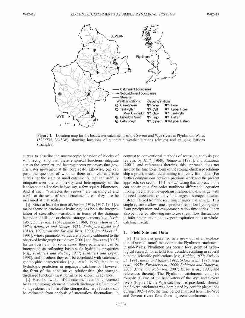
[6] The analysis presented here grew out of an explora-tion of rainfall-runoff behavior at the Plynlimon catchmentsin mid-Wales. Plynlimon has been a focal point of hydro-logical research for at least four decades, resulting in severalhundred scientific publications [e.g., Calder, 1977; Kirby etal., 1991; Beven and Binley, 1992; Sklash et al., 1996; Nealet al., 1997b; Kirchner et al., 2000; Robinson and Dupeyrat,2005; Marc and Robinson, 2007; Kirby et al., 1997, andreferences therein]. The Plynlimon catchments compriseroughly 20 km2 of the headwaters of the Wye and Severnrivers (Figure 1); the Wye catchment is grassland, whereasthe Severn catchment was dominated by conifer plantationsduring 1992–1996, the time period analyzed here. The Wyeand Severn rivers flow from adjacent catchments on the

Figure 1. Location map for the headwater catchments of the Severn and Wye rivers at Plynlimon, Wales(52�270N, 3�430W), showing locations of automatic weather stations (circles) and gauging stations(triangles).

2 of 34

W02429 KIRCHNER: CATCHMENTS AS SIMPLE DYNAMICAL SYSTEMS W02429

same upland massif, predominantly composed of Ordovi-cian and Silurian mudstones, sandstones, shales, and slates,and generally considered to be watertight [Kirby et al.,1991]. Although borehole observations have shown clearevidence for extensive groundwater circulation throughfractures down to depths of tens of meters [Neal et al.,1997a; Shand et al., 2005], no evidence of substantialintercatchment groundwater flow has been reported. Thesoil mantles at both catchments are dominated by blanketpeats >40 cm thick at higher altitudes, podzols at loweraltitudes, and valley bottom alluvium, peat, and stagnohu-mic gleys along the stream channels [Kirby et al., 1991].[7] The climate of Plynlimon is cool and humid; monthly

mean temperatures are typically 2–3�C in winter and 11�–13�C in summer, and annual precipitation is roughly 2500–2600 mm/a, of which approximately 500 mm/a is lost toevapotranspiration and 2000–2100 mm/a runs off as streamdischarge (Table 1). Precipitation varies seasonally, averag-ing 280–300 mm/month during the winter (December/January/February) but only 135–155 mm/month duringthe summer (June/July/August). Rainfall is frequent; morethan 1 mm of rainfall occurs on about 45% of summer daysand over 60% of winter days. Frost can occur in any monthof the year, but snow accounts for only about 5% of totalannual precipitation, and persistent snow cover is rare[Kirby et al., 1991].[8] Precipitation and streamflow have been measured

continuously at Plynlimon since the 1970s by the Centrefor Ecology and Hydrology (formerly the Institute ofHydrology). In addition to a network of ground-levelstorage rain gauges that are read monthly, the Severn andWye catchments are each outfitted with a pair of automaticweather stations, one near the bottom of each catchment andone near the top (circles, Figure 1). These weather stationsprovide hourly records of precipitation, as well as incomingsolar and net radiation, wet and dry bulb temperature, andwind speed and direction, allowing estimation of potentialevapotranspiration via the Penman-Monteith method.Streamflow is measured at 15-min intervals by a trapezoidalcritical depth flume on the Severn and a Crump weir onthe Wye, as well as by flumes on eight tributary streams(triangles, Figure 1).[9] This paper uses data from the four automatic weather

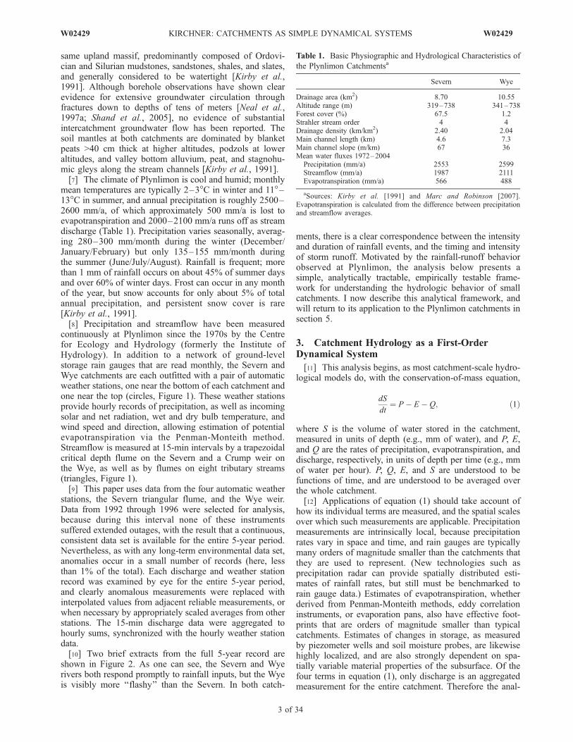
stations, the Severn triangular flume, and the Wye weir.Data from 1992 through 1996 were selected for analysis,because during this interval none of these instrumentssuffered extended outages, with the result that a continuous,consistent data set is available for the entire 5-year period.Nevertheless, as with any long-term environmental data set,anomalies occur in a small number of records (here, lessthan 1% of the total). Each discharge and weather stationrecord was examined by eye for the entire 5-year period,and clearly anomalous measurements were replaced withinterpolated values from adjacent reliable measurements, orwhen necessary by appropriately scaled averages from otherstations. The 15-min discharge data were aggregated tohourly sums, synchronized with the hourly weather stationdata.[10] Two brief extracts from the full 5-year record are

shown in Figure 2. As one can see, the Severn and Wyerivers both respond promptly to rainfall inputs, but the Wyeis visibly more ‘‘flashy’’ than the Severn. In both catch-

ments, there is a clear correspondence between the intensityand duration of rainfall events, and the timing and intensityof storm runoff. Motivated by the rainfall-runoff behaviorobserved at Plynlimon, the analysis below presents asimple, analytically tractable, empirically testable frame-work for understanding the hydrologic behavior of smallcatchments. I now describe this analytical framework, andwill return to its application to the Plynlimon catchments insection 5.

3. Catchment Hydrology as a First-OrderDynamical System

[11] This analysis begins, as most catchment-scale hydro-logical models do, with the conservation-of-mass equation,

dS

dt¼ P � E � Q; ð1Þ

where S is the volume of water stored in the catchment,measured in units of depth (e.g., mm of water), and P, E,and Q are the rates of precipitation, evapotranspiration, anddischarge, respectively, in units of depth per time (e.g., mmof water per hour). P, Q, E, and S are understood to befunctions of time, and are understood to be averaged overthe whole catchment.[12] Applications of equation (1) should take account of

how its individual terms are measured, and the spatial scalesover which such measurements are applicable. Precipitationmeasurements are intrinsically local, because precipitationrates vary in space and time, and rain gauges are typicallymany orders of magnitude smaller than the catchments thatthey are used to represent. (New technologies such asprecipitation radar can provide spatially distributed esti-mates of rainfall rates, but still must be benchmarked torain gauge data.) Estimates of evapotranspiration, whetherderived from Penman-Monteith methods, eddy correlationinstruments, or evaporation pans, also have effective foot-prints that are orders of magnitude smaller than typicalcatchments. Estimates of changes in storage, as measuredby piezometer wells and soil moisture probes, are likewisehighly localized, and are also strongly dependent on spa-tially variable material properties of the subsurface. Of thefour terms in equation (1), only discharge is an aggregatedmeasurement for the entire catchment. Therefore the anal-

Table 1. Basic Physiographic and Hydrological Characteristics of

the Plynlimon Catchmentsa

Severn Wye

Drainage area (km2) 8.70 10.55Altitude range (m) 319–738 341–738Forest cover (%) 67.5 1.2Strahler stream order 4 4Drainage density (km/km2) 2.40 2.04Main channel length (km) 4.6 7.3Main channel slope (m/km) 67 36Mean water fluxes 1972–2004

Precipitation (mm/a) 2553 2599Streamflow (mm/a) 1987 2111Evapotranspiration (mm/a) 566 488

aSources: Kirby et al. [1991] and Marc and Robinson [2007].Evapotranspiration is calculated from the difference between precipitationand streamflow averages.

W02429 KIRCHNER: CATCHMENTS AS SIMPLE DYNAMICAL SYSTEMS

3 of 34

W02429

ysis presented here explores what one can learn aboutcatchment processes from fluctuations in streamflow, with-out assuming that measurements of precipitation or evapo-transpiration are spatially representative. The analysis alsomakes no use of direct measurements of changes in storage,because they are often unavailable.[13] This analysis makes the fundamental assumption that

the discharge in the stream, Q, depends solely on theamount of water stored in the catchment, S. That is, theanalysis assumes that there is some storage-discharge func-tion f(S) such that

Q ¼ f Sð Þ: ð2Þ

This premise is not valid in every catchment, but in manycases it can be a useful approximation, and it is an essentialassumption in the analysis that follows. Of course, in anycatchment some fraction of stream discharge may becontrolled by processes other than the release of waterfrom storage. Two obvious examples are direct precipitationonto the stream surface itself, and precipitation onto areas

that are impermeable or saturated and are directly connectedto the stream. These processes will route precipitationdirectly to discharge as bypassing flow, rather than adding itto subsurface storage. The analysis presented here does notrequire that bypassing flow is entirely absent, but assumesthat it is not a dominant component of discharge. If, instead,discharge is dominated by bypassing flow, the approachpresented here may fail, because processes such as channelrouting (which are not treated in detail here) may dominatethe runoff response. A method for assessing the quantitativesignificance of bypassing flow is presented in section 15.4.[14] The premise that discharge depends on storage is

broadly consistent with the smaller-scale governing equa-tions that drive subsurface transport. For example, the flowof water downward through the unsaturated zone is con-trolled by its matric potential and hydraulic conductivity,which are both steep nonlinear functions of water content.Flow in the saturated zone depends on the slope of the watertable, which varies with storage in the saturated zone, andon the saturated hydraulic conductivity, which varies as afunction of depth; thus transmissivity also depends on the

Figure 2. Time series of hourly rainfall (gray) and discharge (solid black curves) for headwaters of theSevern and Wye rivers during 20-day periods in (a, b) December 1993 and (c, d) March 1994. Rainfalltime series recorded in the two catchments are similar but not identical. Wye flows are more responsive tostorm events than Severn flows. Flows in both rivers generally increase when the catchment mass balanceis positive (rainfall flux is higher than discharge) and decrease when the mass balance is negative (rainfallflux is lower than discharge). As a result, flow peaks in both streams occur at the end of rainfall events, asrainfall fluxes drop below runoff fluxes and the catchment mass balance turns negative. This behavior isconsistent with the simple first-order dynamical system described in equations (1) and (2).

4 of 34


total storage in the saturated zone. As a result, streamdischarge is often a steep nonlinear function of groundwaterlevels in the surrounding catchment [e.g., Laudon et al.,2004, Figure 6]. Many of the processes and rate coefficientsthat control water flow in the subsurface are strongly, andnonlinearly, dependent on storage.[15] Nonetheless it is not clear how these nonlinear

relationships, which may differ from point to point acrossthe landscape, will combine to create a storage-dischargerelationship for the catchment as a whole. For this reason,my approach assumes no particular functional form for thestorage-discharge relationship f(S), instead allowing boththe form of f(S) and its coefficients to be estimated directlyfrom runoff time series data. I assume only that Q is anincreasing single-valued function of S (dQ/dS > 0 for all Qand S), and thus that the storage-discharge function isinvertible. Thus the discharge in the stream provides animplicit measure of the volume of water stored in thecatchment:

S ¼ f �1 Qð Þ: ð3Þ

Equations (1) and (2) form a first-order dynamical system,in which P, Q, E, and S are all understood to be functions oftime. This dynamical system would be particularly simple ifQ were a linear function of S. The properties of such linearsystems have been extensively studied in hydrology, but ingeneral Q will be a nonlinear function of S, resulting in aricher spectrum of possible behaviors. This more generalnonlinear case is the focus of the analysis presented here.[16] Regardless of the form that f(S) takes, the structure of

the dynamical system directly yields an important inferenceconcerning catchment storm response. Because Q is a func-tion of S alone, storage (and thus discharge) will be ris-ing whenever P � E > Q, and falling whenever Q > P � E.The peak discharge (dQ/dt = 0) will coincide with thepeak storage (dS/dt = 0), which will occur when Q = P � E.During storm events, the time of peak rainfall will gener-ally occur during the rising limb of the hydrograph (whenP � E > Q and thus dS/dt > 0 and dQ/dt > 0). Because thepeak rainfall corresponds to rising flow, which by definitionwill occur before the peak discharge, the peak flow will lagthe peak rainfall, even in the absence of any travel time delaysfor pulses of stormflow to reach the weir. Furthermore, thepeak flow will occur as the rainfall rate falls below discharge,and thus the mass balance (equation (1)) turns negative.[17] The Severn and Wye rivers exhibit this pattern of

behavior, as Figure 2 shows. The Wye is somewhat moreresponsive than the Severn to rainfall inputs, but both catch-ments behave as the dynamical system of equations (1) and(2) would predict: when rainfall fluxes exceed streamflowfluxes (and thus the catchment mass balance is positive),discharge increases, and when streamflow exceeds rainfall(and thus the mass balance is negative), discharge decreases.Peak flows occur as rainfall events are ending, when rainfallfluxes drop below streamflow fluxes (and thus the massbalance changes sign). Thus the lag to peak is determinedprimarily by the duration of storm events; it is not a fixedcharacteristic time scale of the catchment.[18] This behavior is inherent in the structure of the

dynamical system described by equations (1) and (2),

because the derivative in equation (1) creates a dynamicalphase lag between fluctuations in precipitation and fluctua-tions in streamflow. If storm runoff were dominated bybypassing flow, and thus changes in catchment storage wereunimportant in the storm response, this phase lag would benegligible. Figure 2 shows that this is not the case atPlynlimon. In addition to this dynamical lag, there mayalso be a travel time lag for stormflows to move down-stream through the channel network. As shown in section 7below, in the Severn and Wye catchments this travel timelag is roughly 1 h, which is less than the width of the blacklines shown in Figure 2.

4. Estimating Catchment Sensitivity to Changesin Storage: Theory

[19] Differentiating equation (2) with respect to time andsubstituting equation (1) directly yields the following dif-ferential equation for the rate of change of dischargethrough time:

dQ

dt¼ dQ

dS

dS

dt¼ dQ

dSP � E � Qð Þ: ð4Þ

The term dQ/dS will be crucial in the analysis that follows;it is the derivative of the storage-discharge relationship f(S),and represents the sensitivity of discharge to changes instorage. Normally, derivatives like dQ/dSwould be expressedin terms of S, but S cannot be directly measured at thecatchment scale for the reasons described in section 3.However, because S is assumed to be a single-valuedfunction of Q, dQ/dS can also be expressed as a function ofQ, here defined as g(Q):

dQ

dS¼ f 0 Sð Þ ¼ f 0 f �1 Qð Þ

� �¼ g Qð Þ: ð5Þ

The function g(Q) will be called the ‘‘sensitivity function’’because it expresses the sensitivity of discharge to changesin storage. Mathematically, it is the implicit differential formof the storage-discharge relationship; it measures howchanges in discharge are related to changes in storage, butit does so as a function of Q (which is directly measurable)rather than S (which is not). This makes it more useful thanthe conventional form f 0(S) for the analysis that follows.Figure 3 illustrates the relationship between the sensitivityfunction g(Q) and the storage-discharge relationship f(S).The function g(Q) can be estimated from observational databy combining equations (5) and (4) to yield

g Qð Þ ¼ dQ

dS¼

dQ=dtdS=dt

¼dQ=dt

P � E � Q; ð6Þ

which implies that the slope of the storage-dischargefunction f(S) can be determined from instantaneousmeasurements of precipitation (P), evapotranspiration (E),discharge (Q), and the rate of change of discharge (dQ/dt).Of the three fluxes (P, E, and Q), discharge can be measuredmore reliably than precipitation or evapotranspiration at thewhole-catchment scale, for the reasons described in section 3above. Therefore equation (6) can be most accuratelyestimated when precipitation and evapotranspiration fluxes


5 of 34

W02429

are small compared to discharge (P � Q and E � Q).Under these conditions, equation (6) is approximated by

g Qð Þ ¼ dQ

dS� � dQ=dt

Q

��P�Q;E�Q

: ð7Þ

Equation (7) implies that one can estimate the sensitivityfunction g(Q) from the time series of Q alone. To do this,one must identify intervals of time when precipitation andevapotranspiration are small compared to discharge, but it isnot necessary to measure either P or E accurately as long astheir rough magnitude compared to Q is known. From thesensitivity function g(Q), one can derive the storage-discharge relationship f(S) by first inverting equation (5),

ZdS ¼

ZdQ

g Qð Þ ; ð8Þ

thus obtaining S as a function of Q, and then by invertingthis function to obtain Q as a function of S.[20] Apart from the requirement that Q = f(S) must be an

increasing function of S (and thus that g(Q) must always bepositive), nothing in the approach outlined here requires f(S)or g(Q) to have any particular mathematical form. Inpractice, g(Q) will be an empirical function that is estimatedfrom streamflow time series data, and it could potentiallyexhibit different functional forms in different catchments. Afew simple functional forms of g(Q) can be integrated andinverted analytically to yield closed-form solutions for f(S).For other functional forms, equation (8) can be solved by

numerical integration in order to construct an empiricalstorage-discharge relationship.

5. Estimating Catchment Sensitivity to Changesin Storage: Practical Details

[21] Implementing this approach in practice requiresidentifying times when precipitation and evapotranspirationfluxes are small enough that equation (6) will be wellapproximated by equation (7). I used two different methodsto identify these low-precipitation, low-ET periods at Plyn-limon, and both yielded similar results. The first approachused the automatic weather station data to estimate potentialevapotranspiration via the Penman-Monteith method. Theestimated potential evapotranspiration does not need toaccurately reflect actual evapotranspiration, but only itsgeneral magnitude, because equation (7) does not requireestimating a mass balance for the catchment, but onlyidentifying times when the mass balance is dominated bydischarge. To implement this approach at Plynlimon, Iselected the hourly records for which discharge was at least10 times larger than both potential evapotranspiration andprecipitation (as measured by the weather station raingauges).[22] The second approach assumes that potential evapo-

transpiration fluxes in humid catchments should be relativelysmall at night, because relative humidity is typically near100% (and thus the vapor pressure deficit is small), andthere is no solar radiation to drive transpiration fluxes (seeFigure 4). To implement this approach at Plynlimon, Iselected the hourly records for nighttime (defined as timesfor which solar flux was less than 1 W/m2 averaged overthe hour in question, the previous hour, and the followinghour), and during which there was also no recorded rainfallwithin the previous 6 h or the following 2 h. Selecting eitherthese rainless night hours, or hours with negligible precipi-tation and potential evapotranspiration (as described above),yields roughly 1600 to 2000 h/a at Plynlimon. Althoughthese two methods for identifying low-precipitation, low-evapotranspiration conditions do not result in exactly thesame records being analyzed (only about half of the recordsoverlap between the two approaches), they both yield sim-ilar results in the analysis that follows. The analysis shownbelow is based on the rainless night hours at the Severn andWye catchments. Figure 5 shows an example of these rain-less nighttime periods, for a short segment of the SevernRiver time series.[23] From hourly streamflow records during periods

when P � Q and E � Q, we can estimate g(Q) in equation(7) by plotting the flow recession rate (�dQ/dt) as afunction of discharge (Q), as shown in Figure 6. Graphslike Figure 6, here termed ‘‘recession plots,’’ were proposedby Brutsaert and Nieber [1977] as an alternative to con-ventional recession curves, in which discharge is plotted asa function of time. Recession plots are particularly appro-priate in the present case, because equation (7) requires low-precipitation, low-evaporation conditions, which usuallyform a highly discontinuous time series (as in Figure 5).Such a discontinuous time series would be ill suited toconventional recession analysis (although others have dealtwith this problem by splicing short intervals together intopseudocontinuous recession curves; see Lamb and Beven[1997] for one such analysis). Recession plots such as

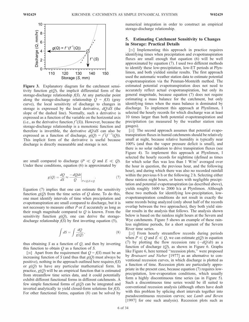
Figure 3. Explanatory diagram for the catchment sensi-tivity function g(Q), the implicit differential form of thestorage-discharge relationship f(S). At any particular pointalong the storage-discharge relationship Q = f(S) (graycurve), the local sensitivity of discharge to changes instorage is expressed by the local derivative, dQ/dS (theslope of the dashed line). Normally, such a derivative isexpressed as a function of the variable on the horizontal axis(i.e., as the derivative function f 0(S)). However, because thestorage-discharge relationship is a monotonic function andtherefore is invertible, the derivative dQ/dS can also beexpressed as a function of discharge, g(Q) = f 0(f �1(Q)).This implicit form of the derivative is useful becausedischarge is directly measurable and storage is not.

6 of 34


Figure 6 provide a general way to display and analyzerecession behavior, without presupposing that the underly-ing data are continuous in time.[24] Following Brutsaert and Nieber [1977], I estimate

the rate of flow recession as the difference in dischargebetween two successive hours, �dQ/dt = (Qt�Dt � Qt)/Dt,and plot this as a function of the average discharge over thetwo hours, (Qt�Dt + Qt)/2. Estimating the terms in this wayavoids any artifactual correlation between Q and �dQ/dt.Because Q and �dQ/dt will both typically span severalorders of magnitude, their relationship to one another canbe best viewed on log-log plots. Figures 6a and 6b showthe relationship between discharge and flow recession forhourly measurements from the Severn and Wye rivers (graydots, Figure 6). In both streams, the rate of flow recessionis roughly a power law function of discharge. Brutsaert and

Nieber [1977] used plots like Figure 6 to define the lowerenvelope of �dQ/dt as a function of Q, under the assump-tion that these points would be least affected by evapotrans-piration, but in practice, much of the spread in �dQ/dt atany particular value of Qmay be due to stochastic variabilityand measurement noise [Rupp and Selker, 2006a], partic-ularly over the short intervals between individual hourlymeasurements. The present approach instead seeks the bestestimate of g(Q) as an average description of the behavior ofthe catchment. This requires estimating the central tendencyof �dQ/dt rather than its lower bound.[25] Accurately estimating g(Q) requires careful attention

to several details. The function g(Q) must correctly describethe relationship between Q and �dQ/dt when they are bothsmall, and log-log plots like Figure 6 expand this domain.The individual hourly data exhibit significant scatter on log

Figure 4. Solar flux, Penman-Monteith potential evapotranspiration, and relative humidity as a functionof time of day for (left) June and (right) December, calculated from hourly measurements at the CefnBrwyn automated weather station in the Wye catchment, 1992–1996. Black dots and lines indicatemeans and standard deviations. During hours of darkness, potential evapotranspiration is nearly zero, andrelative humidity is close to 100%.


7 of 34

W02429

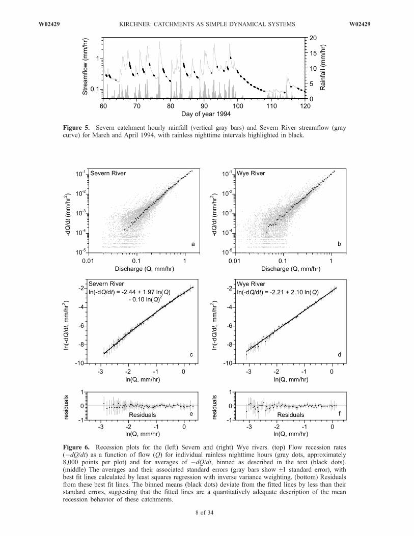
Figure 5. Severn catchment hourly rainfall (vertical gray bars) and Severn River streamflow (graycurve) for March and April 1994, with rainless nighttime intervals highlighted in black.

Figure 6. Recession plots for the (left) Severn and (right) Wye rivers. (top) Flow recession rates(�dQ/dt) as a function of flow (Q) for individual rainless nighttime hours (gray dots, approximately8,000 points per plot) and for averages of �dQ/dt, binned as described in the text (black dots).(middle) The averages and their associated standard errors (gray bars show ±1 standard error), withbest fit lines calculated by least squares regression with inverse variance weighting. (bottom) Residualsfrom these best fit lines. The binned means (black dots) deviate from the fitted lines by less than theirstandard errors, suggesting that the fitted lines are a quantitatively adequate description of the meanrecession behavior of these catchments.

8 of 34


axes, particularly at discharges below about 0.1 mm/h. Thisscatter could arise from at least four sources: (1) randommeasurement noise, (2) coarse graining due to the finitediscretization of discharge measurements, and thus of cal-culated flow recession rates (as is visually evident from thehorizontal stripes in Figures 6a and 6b), (3) effects of anyprecipitation or evapotranspiration that may occur but betoo small to be directly measurable, and (4) differencesbetween the structure of the real-world catchment and theidealized dynamical system hypothesized here. Noise aris-ing from any of these sources should introduce more scatterin the log of �dQ/dt at times when Q and �dQ/dt are small,as Figures 6a and 6b show.[26] On a log scale, this scatter can introduce a bias, since

fluctuations toward zero are larger in log units than equivalentfluctuations away from zero. Indeed, at lowQ, there are manypoints for which discharge is constant or increasing, and thus�dQ/dt for these points cannot be plotted on a log axis at all.It might seem logical to simply exclude such points from theanalysis, under the assumption that any such points cannotcorrespond to flow recession. However, many such pointsmay represent random fluctuations around an average reces-sion trend. Therefore they should not be excluded, becausepreferentially excluding random deviations in one directionbut not the other would lead to biased estimates of the averagerecession rate �dQ/dt at any given Q.[27] Instead, the scatter at low Q must be properly taken

into account in order to estimate the functional relationshipbetween �dQ/dt and Q. In Figure 6, I do this by binning theindividual hourly data points into ranges of Q, and thencalculating the mean and standard error for �dQ/dt and Qwithin each bin (including values of �dQ/dt � 0, whichcannot be displayed on log axes). These means are the blackdots in Figure 6. Working from the highest values of Q tothe lowest, I delimit bins that span at least 1% of thelogarithmic range in Q, and that include enough points thatthe standard error of �dQ/dt within the bin is less than halfof its mean. The criterion std.err.(�dQ/dt) � mean(dQ/dt)/2is a first-order Taylor approximation to the criterionstd.err.(ln(�dQ/dt)) � 0.5, which cannot be directly evalu-ated when dQ/dt has both positive and negative values. Thebinned averages reflect the average recession rate �dQ/dt ateach flow rate Q, without being unduly influenced by thestochastic scatter in �dQ/dt when Q is small.[28] I then fit smooth curves to the binned means (black

dots) using least squares regression, weighted by inversevariance (that is, by the reciprocal of the square of the standarderrors of each binned average). This approach keeps highlyuncertain points from exerting too much influence on theregression. This approach also yields the maximum-likelihoodestimator for the best fit curve, if the deviations of the blackdots from the true relationship are approximately normal. Thisis likely to be the case, because according to the central limittheorem, the errors in the binned means (black dots) should bedistributed almost normally even if the individual measure-ments (gray dots) are not, since each black dot is typicallycalculated by averaging many individual points. As theresidual plots at the bottom of Figure 6 show, the best fitcurves fall within one standard error of nearly all of the binnedmeans, implying that they capture nearly all of the systematicrelationship between ln(�dQ/dt) and ln(Q). If, on the otherhand, the best fit curves fell outside the error bars of many of

the binned means, this would indicate that the curves wereincorrectly estimated or were not flexible enough to follow thestructural relationship between ln(�dQ/dt) and ln(Q).[29] In the absence of a strong theoretical expectation for

the storage-discharge relationship to have a particular func-tional form, one must choose an empirical function to fit tothe binned means in Figure 6. To fit the black dots inFigure 6, I chose a quadratic curve because it is both flexibleenough to follow the major features of the data and smoothenough to permit modest extrapolation beyond the range ofthe black dots. This quadratic function leads directly to anexpression for g(Q) as a quadratic in logs,

ln g Qð Þð Þ ¼ ln� dQ=dt

Q

��P�Q;E�Q

!� c1 þ c2 ln Qð Þ þ c3 ln Qð Þð Þ2;

ð9Þ

with parameter values of c1 = �2.439 ± 0.017, c2 = 0.966 ±0.035, and c3 = �0.100 ± 0.016 for the Severn River, andparameter values of c1 = �2.207 ± 0.028, c2 = 1.099 ±0.048, and c3 = �0.002 ± 0.018 for the Wye River, obtainedby polynomial least squares regression. The coefficient c2 isone less than the slope of the log-log plots in Figure 6,owing to the factor of Q in the denominator of equation (9).[30] The fitted curves for the Severn and Wye rivers look

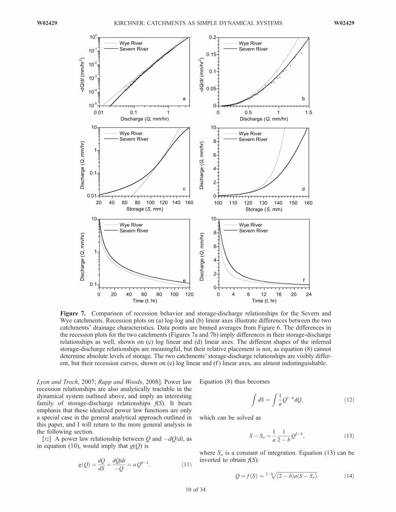
similar in Figure 6, although when they are overlain on oneanother, small differences are visually apparent (Figures 7aand 7b). Nonetheless, when these fitted curves are trans-formed to storage-discharge relationships, they are visuallyquite distinct (Figures 7c and 7d). Notably, the Wye River’sstorage-discharge relationship is more sharply curved thanthe Severn’s, which is broadly consistent with the Wye’smore abrupt response to precipitation, as shown in Figure 2.Integrating these storage-discharge relationships yields the-oretical recession curves (discharge as a function of time);as Figures 7e and 7f show, the recession curves for the twocatchments are visually similar, despite the obvious differ-ences between their storage-discharge relationships. Thisobservation suggests that conventional analyses of recessioncurves may not detect important differences in storage-discharge relationships between catchments. These differ-ences are, however, apparent from the analysis outlinedabove.

6. PowerLawRelationshipsBetweenQand�dQ/dt:An Idealized Approximation

[31] Log-log recession plots such as Figure 6 are oftenapproximately linear, suggesting a power law relationshipbetween discharge Q and the recession rate �dQ/dt,

� dQ

dt¼ aQb; ð10Þ

where b is the log-log slope of the best fit line. Followingthe fundamental contributions of Horton [1941] andBrutsaert and Nieber [1977], this power law recessionbehavior has been used to characterize catchments in anumber of ways, usually based on a nonlinear reservoirmodel or a Boussinesq representation of flow in thesubsurface [e.g., Troch et al., 1993; Brutsaert and Lopez,1998; Tague and Grant, 2004; Rupp and Selker, 2006b;


9 of 34

W02429

Lyon and Troch, 2007; Rupp and Woods, 2008]. Power lawrecession relationships are also analytically tractable in thedynamical system outlined above, and imply an interestingfamily of storage-discharge relationships f(S). It bearsemphasis that these idealized power law functions are onlya special case in the general analytical approach outlined inthis paper, and I will return to the more general analysis inthe following section.[32] A power law relationship between Q and �dQ/dt, as

in equation (10), would imply that g(Q) is

g Qð Þ ¼ dQ

dS¼ dQ=dt

�Q¼ aQb�1: ð11Þ

Equation (8) thus becomes

ZdS ¼

Z1

aQ1�bdQ; ð12Þ

which can be solved as

S � So ¼1

a

1

2� bQ2�b; ð13Þ

where So is a constant of integration. Equation (13) can beinverted to obtain f(S):

Q ¼ f Sð Þ ¼ 2�bffiffiffiffiffiffiffiffiffiffiffiffiffiffiffiffiffiffiffiffiffiffiffiffiffiffiffiffiffiffiffiffiffiffi2� bð Þa S � Soð Þ

p: ð14Þ

Figure 7. Comparison of recession behavior and storage-discharge relationships for the Severn andWye catchments. Recession plots on (a) log-log and (b) linear axes illustrate differences between the twocatchments’ drainage characteristics. Data points are binned averages from Figure 6. The differences inthe recession plots for the two catchments (Figures 7a and 7b) imply differences in their storage-dischargerelationships as well, shown on (c) log linear and (d) linear axes. The different shapes of the inferredstorage-discharge relationships are meaningful, but their relative placement is not, as equation (8) cannotdetermine absolute levels of storage. The two catchments’ storage-discharge relationships are visibly differ-ent, but their recession curves, shown on (e) log linear and (f ) linear axes, are almost indistinguishable.

10 of 34


In equation (10) and thus also in equation (14), thedimensions of the constant a will vary with b, aslength(b�1)/(2�b)time1/(2�b), for dimensional consistency.Equation (14) can also be rewritten in a more dimensionallystraightforward form as

Q ¼ f Sð Þ ¼ Qref S � Soð Þ=k1ð Þ1= 2�bð Þ; ð15Þ

where Qref is an arbitrary reference discharge, and thescaling constant k1 = (Qref

2�b)/[(2 � b)a] has the samedimensions as storage.[33] Equations (14) and (15) have three classes of solu-

tions, and in each case the constant of integration So meanssomething different. If b < 2, equation (14) yields Q as apower function of S, with So representing the residualstorage remaining in the catchment when discharge dropsto zero. In the special case where b = 1, f(S) is linear and theconventional results for linear reservoirs (such as log linearrecession curves) are obtained. As b increases from 1toward 2, f(S) becomes an increasingly steep power func-tion, with the exponent 1/(2 � b) in equation (15) approach-ing infinity as b approaches 2.[34] When b = 2, the solution to equation (8) is an

exponential function,

Q ¼ f Sð Þ ¼ Qref ea S�Soð Þ; ð16Þ

where So now represents the value of storage when Q = Qref.Note that in equation (16), there will be some finitedischarge at all values of S, allowing storage to declineindefinitely.[35] When b is greater than 2, equations (14) and (15)

become hyperbolic, and the meaning of So changes signif-icantly. Values of b > 2 imply that 2 � b is negative, soequations (14) and (15) will yield imaginary values of Qunless S is less than So. Thus when b > 2, So is no longer thelower bound to storage (at which discharge would decreaseto zero); instead, So is the upper limit to storage, unreach-able in practice, at which discharge would become infinite(for a different but mathematically equivalent interpretation,see Rupp and Woods [2008]). When b > 2, the behavior ofequation (15) can be seen more clearly if it is rewritten as

Q ¼ f Sð Þ ¼ Qref

So � Sð Þ=k2ð Þ1= b�2ð Þ ; ð17Þ

where Qref is again an arbitrary reference discharge, andk2 = �k1 = (Qref

2�b)/[a(b � 2)] again has the samedimensions as storage. Equation (17) is equivalent to (15),but is easier to understand in this form because the scalingconstant k2 and the exponent 1/(b � 2) are both positivewhen b > 2, whereas in equation (15) the scaling constant k1and the exponent 1/(2 � b) would both be negative.[36] The best fit values of b, obtained from Figure 6 by

linear regression, are b = 2.168 ± 0.017 for the Severn Riverand b = 2.103 ± 0.015 for the Wye River. (These valuesdiffer somewhat from the linear terms in the polynomialregressions reported above, because of collinearity betweenthe linear and quadratic terms in those polynomial expres-sions). These best fit values of b both exceed b = 2 by morethan six standard errors. Thus, to the extent that the Severn

and Wye catchments could both be approximated by powerlaw recession plots, they would both appear to exhibit thehyperbolic behavior described by equation (17). Thus thehyperbolic solution represented by equation (17) may bemore than just a mathematical oddity, and may be useful forunderstanding the behavior of flashy hydrologic systems.[37] Figure 8 shows log-log recession plots (similar to

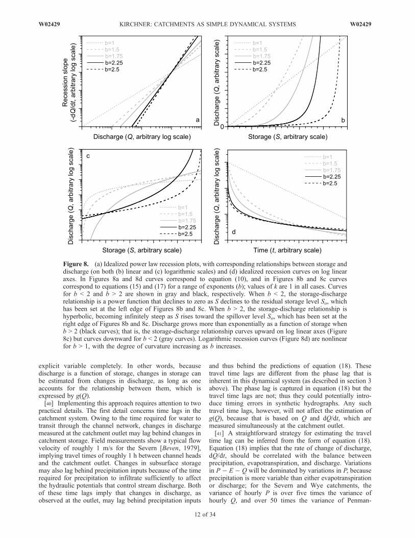
Figure 6) for a range of exponents b, along with thecorresponding storage-discharge relationships, and theresulting recession curves as functions of time. AsFigure 8b illustrates, the storage-discharge relationshipbecomes dramatically more nonlinear as b increases. Whenb is greater than 2, discharge increases more than exponen-tially as a function of storage; that is, the log of Q curvesupward as a function of S (Figure 8c). Figure 8d showshypothetical recession curves of log(Q) as a function oftime, derived by integrating equations (1) and (2), or,alternatively, equations (4) and (11). As Figure 8d shows,these logarithmic recession curves become increasinglynonlinear as b increases, and are very sharply curved whenb is greater than 2.

7. Simulating HydrographsFrom Storage-Discharge Relationships

[38] From the preceding discussion, one can devise astraightforward strategy for rainfall-runoff modeling usingthe methods outlined above. The discharge sensitivityfunction g(Q) could be numerically integrated (or analyti-cally integrated if its functional form is simple enough),yielding the storage-discharge relationship f(S). One couldthen iteratively simulate the simple dynamical systemformed by Q = f(S) and dS/dt = P � E � Q, initializingthis system at some beginning time step using S = f �1(Q).From time series of P and E, one could then simulate thetime series of Q.[39] However, because Q is a differentiable and invertible

function of S, the dynamical system of equations (1) and (2)can be solved in a more elegant way that does not requireexplicitly accounting for storage at all. Combining equa-tions (4) and (5), one directly obtains

dQ

dt¼ dQ

dS

dS

dt¼ g Qð Þ P � E � Qð Þ; ð18Þ

which is a first-order nonlinear differential equation for Qthat depends only on the values of P and E over time.Therefore one can simulate the streamflow hydrographdirectly from time series of P and E by integrating equation(18) through time, given only a single value of Q to initializethe integration. This approach is more direct than explicitlysolving equations (1) and (2), for two reasons. First, it avoidsthe need to know the antecedent moisture conditions at thebeginning of a simulation. Second, and more significantly, itavoids the potentially difficult process of inferring thestorage-discharge relationship f(S) from the sensitivityfunction g(Q). Where, one might ask, has the storagevariable gone? Note that in the conservation of massequation, storage appears only as its time derivative; thatis, one never needs to know the value of storage, but only itsrate of change through time. Thus one can use a differentialform of the storage-discharge function. If one uses theimplicit differential form, g(Q), one can eliminate S as an


11 of 34

W02429

explicit variable completely. In other words, becausedischarge is a function of storage, changes in storage canbe estimated from changes in discharge, as long as oneaccounts for the relationship between them, which isexpressed by g(Q).[40] Implementing this approach requires attention to two

practical details. The first detail concerns time lags in thecatchment system. Owing to the time required for water totransit through the channel network, changes in dischargemeasured at the catchment outlet may lag behind changes incatchment storage. Field measurements show a typical flowvelocity of roughly 1 m/s for the Severn [Beven, 1979],implying travel times of roughly 1 h between channel headsand the catchment outlet. Changes in subsurface storagemay also lag behind precipitation inputs because of the timerequired for precipitation to infiltrate sufficiently to affectthe hydraulic potentials that control stream discharge. Bothof these time lags imply that changes in discharge, asobserved at the outlet, may lag behind precipitation inputs

and thus behind the predictions of equation (18). Thesetravel time lags are different from the phase lag that isinherent in this dynamical system (as described in section 3above). The phase lag is captured in equation (18) but thetravel time lags are not; thus they could potentially intro-duce timing errors in synthetic hydrographs. Any suchtravel time lags, however, will not affect the estimation ofg(Q), because that is based on Q and dQ/dt, which aremeasured simultaneously at the catchment outlet.[41] A straightforward strategy for estimating the travel

time lag can be inferred from the form of equation (18).Equation (18) implies that the rate of change of discharge,dQ/dt, should be correlated with the balance betweenprecipitation, evapotranspiration, and discharge. Variationsin P � E � Q will be dominated by variations in P, becauseprecipitation is more variable than either evapotranspirationor discharge; for the Severn and Wye catchments, thevariance of hourly P is over five times the variance ofhourly Q, and over 50 times the variance of Penman-

Figure 8. (a) Idealized power law recession plots, with corresponding relationships between storage anddischarge (on both (b) linear and (c) logarithmic scales) and (d) idealized recession curves on log linearaxes. In Figures 8a and 8d curves correspond to equation (10), and in Figures 8b and 8c curvescorrespond to equations (15) and (17) for a range of exponents (b); values of k are 1 in all cases. Curvesfor b < 2 and b > 2 are shown in gray and black, respectively. When b < 2, the storage-dischargerelationship is a power function that declines to zero as S declines to the residual storage level So, whichhas been set at the left edge of Figures 8b and 8c. When b > 2, the storage-discharge relationship ishyperbolic, becoming infinitely steep as S rises toward the spillover level So, which has been set at theright edge of Figures 8b and 8c. Discharge grows more than exponentially as a function of storage whenb > 2 (black curves); that is, the storage-discharge relationship curves upward on log linear axes (Figure8c) but curves downward for b < 2 (gray curves). Logarithmic recession curves (Figure 8d) are nonlinearfor b > 1, with the degree of curvature increasing as b increases.

12 of 34


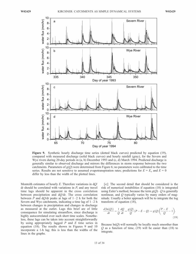
Monteith estimates of hourly E. Therefore variations in dQ/dt should be correlated with variations in P, and any traveltime lags should be apparent in the cross correlationbetween precipitation and dQ/dt. The cross correlationbetween P and dQ/dt peaks at lags of 1–2 h for both theSevern and Wye catchments, indicating a time lag of 1–2 hbetween changes in precipitation and changes in dischargeas measured at the outlet. Lags this brief are of littleconsequence for simulating streamflow, since discharge ishighly autocorrelated over such short time scales. Nonethe-less, these lags can be taken into account straightforwardlyby using appropriately lagged P and E time series inequation (18). The results shown in Figures 9 and 10incorporate a 1-h lag; this is less than the widths of thelines in the graphs.

[42] The second detail that should be considered is therisk of numerical instabilities if equation (18) is integratedusing Euler’s method, because the term g(Q) Q is generallynonlinear, and Q typically varies by many orders of mag-nitude. Usually a better approach will be to integrate the logtransform of equation (18),

d ln Qð Þð Þdt

¼ 1

Q

dQ

dt¼ g Qð Þ

QP � E � Qð Þ ¼ g Qð Þ P � E

Q� 1

:

ð19Þ

Because ln(Q) will normally be locally much smoother thanQ as a function of time, (19) will be easier than (18) tointegrate.

Figure 9. Synthetic hourly discharge time series (dotted black curves) predicted by equation (19),compared with measured discharge (solid black curves) and hourly rainfall (gray), for the Severn andWye rivers during 20-day periods in (a, b) December 1993 and (c, d) March 1994. Predicted discharge isgenerally similar to observed discharge and mirrors the differences in storm response between the twocatchments. Parameters of g(Q) were determined from Figure 6; no parameters were calibrated to the timeseries. Results are not sensitive to assumed evapotranspiration rates; predictions for E = Eo and E = 0differ by less than the width of the plotted lines.


13 of 34

W02429

[43] As Figures 9 and 10 show, this approach producessynthetic hydrographs that closely resemble the streamflowtime series at Plynlimon. The hydrographs shown inFigures 9 and 10 were synthesized by iterating (19) on anhourly time step, using fourth-order Runge-Kutta integra-tion. The g(Q) functions for the two catchments wereobtained directly from Figure 6, and were not calibratedto the time series. The only calibration consisted of rescal-ing the Penman-Monteith potential evapotranspiration esti-mates Eo by an adjustable coefficient kE to obtain theevapotranspiration time series E = kE Eo; a single value ofkE was fitted for the entire 5-year period 1992–1996. Theanalysis contains no other adjustable coefficients.[44] As Figure 9 shows, the synthetic hydrographs cor-

rectly predict the general magnitude and timing of stormresponse at the two catchments, and generally reproduce theshape of the stormflow recessions. The synthetic hydro-graphs even reproduce the subtle differences in stormresponse between the two catchments; stormflow peaks inthe Wye River are higher and narrower, with somewhatmore rapid recessions. Note in particular that no parameterswere adjusted to fit the stormflow periods shown in Figure 9.The two periods shown in Figure 9 correspond to relativelywet conditions, when the synthetic hydrographs (dashedlines) are insensitive to kE and are therefore effectively freeof any direct calibration. Nonetheless the results shown inFigure 9 compare well with much more complex modelsthat have been applied to the Plynlimon catchments, withextensive parameter calibration [e.g., Rogers et al., 1985;Bathurst, 1986].[45] Catchment hydrologic models often perform rela-

tively well in wet conditions, but break down during drierconditions. A model’s low-flow characteristics are con-cealed when hydrographs are plotted on linear axes as inFigure 9, because flow variations spanning orders of mag-nitude (i.e., all except the highest flows) will appear asnearly horizontal lines close to the bottom of the plot. Forthis reason it is diagnostic to also compare synthetic and

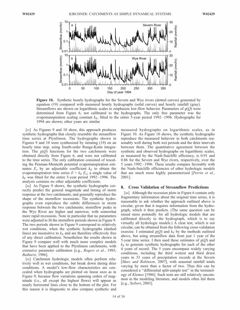
measured hydrographs on logarithmic scales, as inFigure 10. As Figure 10 shows, the synthetic hydrographsreproduce the measured behavior in both catchments rea-sonably well during both wet periods and the drier intervalsbetween them. The quantitative agreement between thesynthetic and observed hydrographs on logarithmic scales,as measured by the Nash-Sutcliffe efficiency, is 0.91 and0.86 for the Severn and Wye rivers, respectively, over the5 years 1992–1996. These results compare favorably withthe Nash-Sutcliffe efficiencies of other hydrologic modelsthat are much more highly parameterized [Perrin et al.,2001].

8. Cross Validation of Streamflow Predictions

[46] Although the recession plots in Figure 6 contain onlyfragmentary information about the original time series, it isreasonable to ask whether the approach outlined above iscircular, given that it requires information from the hydro-graph, which it then predicts. (The same question can beraised more pointedly for all hydrologic models that arecalibrated directly to the hydrograph, which is to sayvirtually all hydrologic models.) A clear test, which is notcircular, can be obtained from the following cross-validationexercise. I estimated g(Q) and kE by the methods outlinedabove, but using streamflow data from just 1 year of the5-year time series. I then used these estimates of g(Q) andkE to generate synthetic hydrographs for each of the other4 years of record. The 5 years encompass widely varyingconditions, including the third wettest and third driestyears in 33 years of precipitation records at the Severn[Marc and Robinson, 2007], with seasonal rainfall totalsvarying by more than a factor of two. Thus this can beconsidered a ‘‘differential split-sample test’’ in the terminol-ogy of Klemes [1986]. Such tests are still relatively uncom-mon in the modeling literature, and models often fail them[e.g., Seibert, 2003].

Figure 10. Synthetic hourly hydrographs for the Severn and Wye rivers (dotted curves) generated byequation (19) compared with measured hourly hydrographs (solid curves) and hourly rainfall (gray).Streamflows are shown on logarithmic scales to emphasize low-flow behavior. Parameters of g(Q) weredetermined from Figure 6, not calibrated to the hydrographs. The only free parameter was theevapotranspiration scaling constant kE, fitted to the entire 5-year period 1992–1996. Hydrographs for1994 are shown; other years are similar.

14 of 34


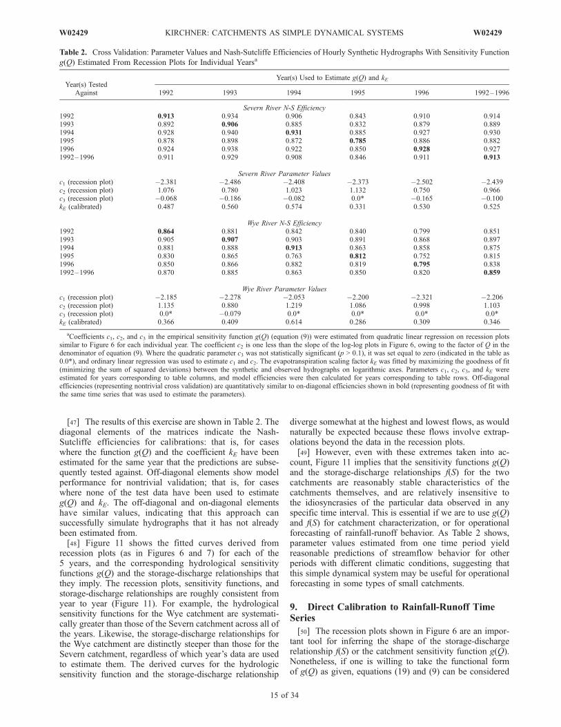
[47] The results of this exercise are shown in Table 2. Thediagonal elements of the matrices indicate the Nash-Sutcliffe efficiencies for calibrations: that is, for caseswhere the function g(Q) and the coefficient kE have beenestimated for the same year that the predictions are subse-quently tested against. Off-diagonal elements show modelperformance for nontrivial validation; that is, for caseswhere none of the test data have been used to estimateg(Q) and kE. The off-diagonal and on-diagonal elementshave similar values, indicating that this approach cansuccessfully simulate hydrographs that it has not alreadybeen estimated from.[48] Figure 11 shows the fitted curves derived from

recession plots (as in Figures 6 and 7) for each of the5 years, and the corresponding hydrological sensitivityfunctions g(Q) and the storage-discharge relationships thatthey imply. The recession plots, sensitivity functions, andstorage-discharge relationships are roughly consistent fromyear to year (Figure 11). For example, the hydrologicalsensitivity functions for the Wye catchment are systemati-cally greater than those of the Severn catchment across all ofthe years. Likewise, the storage-discharge relationships forthe Wye catchment are distinctly steeper than those for theSevern catchment, regardless of which year’s data are usedto estimate them. The derived curves for the hydrologicsensitivity function and the storage-discharge relationship

diverge somewhat at the highest and lowest flows, as wouldnaturally be expected because these flows involve extrap-olations beyond the data in the recession plots.[49] However, even with these extremes taken into ac-

count, Figure 11 implies that the sensitivity functions g(Q)and the storage-discharge relationships f(S) for the twocatchments are reasonably stable characteristics of thecatchments themselves, and are relatively insensitive tothe idiosyncrasies of the particular data observed in anyspecific time interval. This is essential if we are to use g(Q)and f(S) for catchment characterization, or for operationalforecasting of rainfall-runoff behavior. As Table 2 shows,parameter values estimated from one time period yieldreasonable predictions of streamflow behavior for otherperiods with different climatic conditions, suggesting thatthis simple dynamical system may be useful for operationalforecasting in some types of small catchments.

9. Direct Calibration to Rainfall-Runoff TimeSeries

[50] The recession plots shown in Figure 6 are an impor-tant tool for inferring the shape of the storage-dischargerelationship f(S) or the catchment sensitivity function g(Q).Nonetheless, if one is willing to take the functional formof g(Q) as given, equations (19) and (9) can be considered

Table 2. Cross Validation: Parameter Values and Nash-Sutcliffe Efficiencies of Hourly Synthetic Hydrographs With Sensitivity Function

g(Q) Estimated From Recession Plots for Individual Yearsa

Year(s) TestedAgainst

Year(s) Used to Estimate g(Q) and kE

1992 1993 1994 1995 1996 1992–1996

Severn River N-S Efficiency1992 0.913 0.934 0.906 0.843 0.910 0.9141993 0.892 0.906 0.885 0.832 0.879 0.8891994 0.928 0.940 0.931 0.885 0.927 0.9301995 0.878 0.898 0.872 0.785 0.886 0.8821996 0.924 0.938 0.922 0.850 0.928 0.9271992–1996 0.911 0.929 0.908 0.846 0.911 0.913

Severn River Parameter Valuesc1 (recession plot) �2.381 �2.486 �2.408 �2.373 �2.502 �2.439c2 (recession plot) 1.076 0.780 1.023 1.132 0.750 0.966c3 (recession plot) �0.068 �0.186 �0.082 0.0* �0.165 �0.100kE (calibrated) 0.487 0.560 0.574 0.331 0.530 0.525

Wye River N-S Efficiency1992 0.864 0.881 0.842 0.840 0.799 0.8511993 0.905 0.907 0.903 0.891 0.868 0.8971994 0.881 0.888 0.913 0.863 0.858 0.8751995 0.830 0.865 0.763 0.812 0.752 0.8151996 0.850 0.866 0.882 0.819 0.795 0.8381992–1996 0.870 0.885 0.863 0.850 0.820 0.859

Wye River Parameter Valuesc1 (recession plot) �2.185 �2.278 �2.053 �2.200 �2.321 �2.206c2 (recession plot) 1.135 0.880 1.219 1.086 0.998 1.103c3 (recession plot) 0.0* �0.079 0.0* 0.0* 0.0* 0.0*kE (calibrated) 0.366 0.409 0.614 0.286 0.309 0.346

aCoefficients c1, c2, and c3 in the empirical sensitivity function g(Q) (equation (9)) were estimated from quadratic linear regression on recession plotssimilar to Figure 6 for each individual year. The coefficient c2 is one less than the slope of the log-log plots in Figure 6, owing to the factor of Q in thedenominator of equation (9). Where the quadratic parameter c3 was not statistically significant (p > 0.1), it was set equal to zero (indicated in the table as0.0*), and ordinary linear regression was used to estimate c1 and c2. The evapotranspiration scaling factor kE was fitted by maximizing the goodness of fit(minimizing the sum of squared deviations) between the synthetic and observed hydrographs on logarithmic axes. Parameters c1, c2, c3, and kE wereestimated for years corresponding to table columns, and model efficiencies were then calculated for years corresponding to table rows. Off-diagonalefficiencies (representing nontrivial cross validation) are quantitatively similar to on-diagonal efficiencies shown in bold (representing goodness of fit withthe same time series that was used to estimate the parameters).


15 of 34

W02429

as a simple four-parameter rainfall-runoff model that canbe directly calibrated to time series of precipitation, evapo-transpiration, and discharge. To test the utility of thisapproach, I jointly calibrated the three coefficients c1, c2,and c3 in equation (9), along with the evapotranspirationscaling factor kE, by minimizing the sum of squared devia-tions between the predicted and observed stream dischargeon logarithmic axes. I calibrated a parameter set for eachyear individually, then used each parameter set to generatestreamflow predictions for the other four years of record.This is the same cross-validation exercise conducted insection 8, except that here all of the parameters were deter-mined by direct calibration against the time series of catch-ment discharge.[51] The results of this cross-validation exercise show

that this simple model performs almost equally well, both inverification tests against the same years that it was calibrat-

ed with (the on-diagonal elements of Table 3) and innontrivial validation tests against different years (the off-diagonal elements of Table 3). These results demonstratethat the model is reasonably robust.[52] A comparison of Tables 2 and 3 shows that, unsur-

prisingly, the model fits the observed streamflow somewhatbetter when all four parameters are calibrated (Table 3) thanwhen just one parameter (kE) is fitted to the streamflow timeseries (Table 2). What is perhaps surprising, however, is thatthe values of all four parameters in Table 3 are consistentacross the different years of calibration. In many hydrolog-ical models, the parameters introduce more degrees offreedom than the data can adequately constrain, with theresult that different combinations of parameters often giveequally good fits to the calibration data (the equifinalityproblem [Beven and Binley, 1992]), and thus the parametervalues are often sensitive to the idiosyncrasies of the

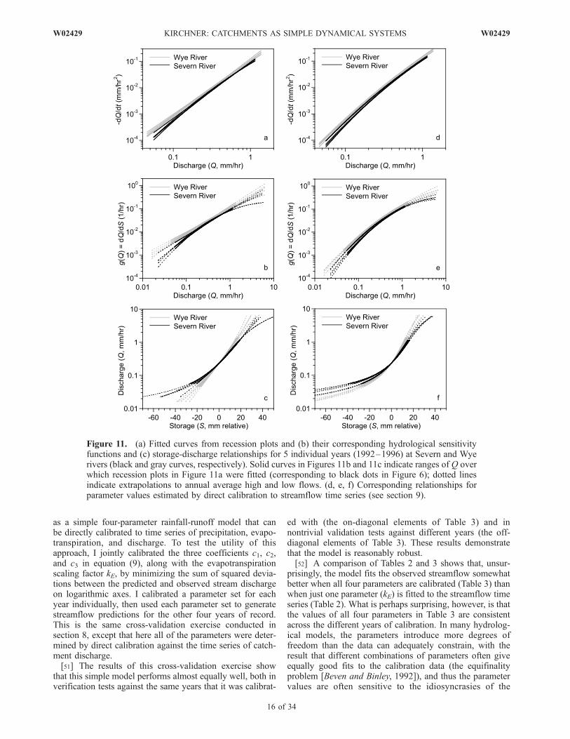
Figure 11. (a) Fitted curves from recession plots and (b) their corresponding hydrological sensitivityfunctions and (c) storage-discharge relationships for 5 individual years (1992–1996) at Severn and Wyerivers (black and gray curves, respectively). Solid curves in Figures 11b and 11c indicate ranges of Q overwhich recession plots in Figure 11a were fitted (corresponding to black dots in Figure 6); dotted linesindicate extrapolations to annual average high and low flows. (d, e, f) Corresponding relationships forparameter values estimated by direct calibration to streamflow time series (see section 9).

16 of 34


calibration data. The values shown in Table 3 indicate thatthis is not the case, suggesting that the model is notoverparameterized.[53] The parameter values obtained by direct calibration

(Table 3) are broadly consistent with those obtained fromthe recession plots (Table 2). Both sets of parametersindicate that the Wye catchment has higher g(Q) valuesand thus is more sensitive to changes in storage than theSevern (Figure 11). Both sets of parameters also indicatethat g(Q) is more strongly curved in the Severn than theWye, implying a somewhat shallower storage-dischargerelationship f(S). However, compared to the coefficientsobtained from the recession plots, the parameter valuesobtained by time series calibration imply greater downwardcurvature (consistently more negative values of c3) in thesensitivity function g(Q) (compare Figures 11b and 11e).This in turn implies that the lower range of the storage-discharge relationship f(S) is flatter (compare Figures 11cand 11f), with the result that long-term streamflow recessionwill be slower under these parameter values.

10. Catchment Characterization: EstimatingCatchment Dynamic Storage

[54] Catchments can be usefully characterized by theirdynamic storage, that is, their variation in storage betweendry and wet periods [e.g., Kirby et al., 1991; Uchida et al.,2006; Spence, 2007]. The size of a catchment’s dynamic

storage provides important insight into both vulnerability toflooding and sustainability of low flows. In principle, itshould be straightforward to estimate dynamic storage bytaking a running integral of the catchment mass balance(equation (1)). In practice, however, this integral willnormally be subject to large errors, as small measurementbiases and uncertainties in P, Q, and E accumulate throughtime.[55] If the catchment is characterized by a robust storage-

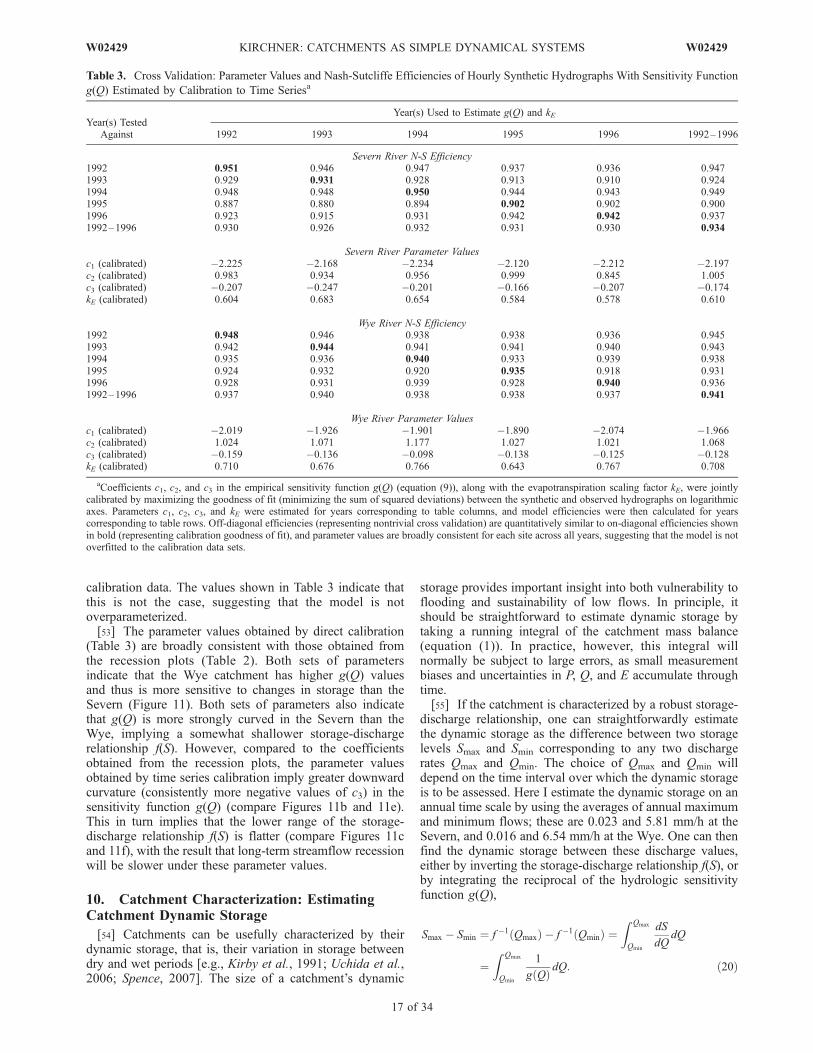
discharge relationship, one can straightforwardly estimatethe dynamic storage as the difference between two storagelevels Smax and Smin corresponding to any two dischargerates Qmax and Qmin. The choice of Qmax and Qmin willdepend on the time interval over which the dynamic storageis to be assessed. Here I estimate the dynamic storage on anannual time scale by using the averages of annual maximumand minimum flows; these are 0.023 and 5.81 mm/h at theSevern, and 0.016 and 6.54 mm/h at the Wye. One can thenfind the dynamic storage between these discharge values,either by inverting the storage-discharge relationship f(S), orby integrating the reciprocal of the hydrologic sensitivityfunction g(Q),

Smax � Smin ¼ f �1 Qmaxð Þ � f �1 Qminð Þ ¼Z Qmax

Qmin

dS

dQdQ

¼Z Qmax

Qmin

1

g Qð Þ dQ: ð20Þ

Table 3. Cross Validation: Parameter Values and Nash-Sutcliffe Efficiencies of Hourly Synthetic Hydrographs With Sensitivity Function

g(Q) Estimated by Calibration to Time Seriesa

Year(s) TestedAgainst

Year(s) Used to Estimate g(Q) and kE

1992 1993 1994 1995 1996 1992–1996

Severn River N-S Efficiency1992 0.951 0.946 0.947 0.937 0.936 0.9471993 0.929 0.931 0.928 0.913 0.910 0.9241994 0.948 0.948 0.950 0.944 0.943 0.9491995 0.887 0.880 0.894 0.902 0.902 0.9001996 0.923 0.915 0.931 0.942 0.942 0.9371992–1996 0.930 0.926 0.932 0.931 0.930 0.934

Severn River Parameter Valuesc1 (calibrated) �2.225 �2.168 �2.234 �2.120 �2.212 �2.197c2 (calibrated) 0.983 0.934 0.956 0.999 0.845 1.005c3 (calibrated) �0.207 �0.247 �0.201 �0.166 �0.207 �0.174kE (calibrated) 0.604 0.683 0.654 0.584 0.578 0.610

Wye River N-S Efficiency1992 0.948 0.946 0.938 0.938 0.936 0.9451993 0.942 0.944 0.941 0.941 0.940 0.9431994 0.935 0.936 0.940 0.933 0.939 0.9381995 0.924 0.932 0.920 0.935 0.918 0.9311996 0.928 0.931 0.939 0.928 0.940 0.9361992–1996 0.937 0.940 0.938 0.938 0.937 0.941

Wye River Parameter Valuesc1 (calibrated) �2.019 �1.926 �1.901 �1.890 �2.074 �1.966c2 (calibrated) 1.024 1.071 1.177 1.027 1.021 1.068c3 (calibrated) �0.159 �0.136 �0.098 �0.138 �0.125 �0.128kE (calibrated) 0.710 0.676 0.766 0.643 0.767 0.708

aCoefficients c1, c2, and c3 in the empirical sensitivity function g(Q) (equation (9)), along with the evapotranspiration scaling factor kE, were jointlycalibrated by maximizing the goodness of fit (minimizing the sum of squared deviations) between the synthetic and observed hydrographs on logarithmicaxes. Parameters c1, c2, c3, and kE were estimated for years corresponding to table columns, and model efficiencies were then calculated for yearscorresponding to table rows. Off-diagonal efficiencies (representing nontrivial cross validation) are quantitatively similar to on-diagonal efficiencies shownin bold (representing calibration goodness of fit), and parameter values are broadly consistent for each site across all years, suggesting that the model is notoverfitted to the calibration data sets.


17 of 34

W02429

As Figure 12 shows, this procedure yields an annualdynamic storage of approximately 98 mm at the Severn and62 mm at the Wye, if the parameters of g(Q) are estimatedfrom the recession plots (Figure 6). If the parameter valuesare estimated by direct calibration to the streamflow timeseries as in section 9 above, the annual dynamic storageestimates are somewhat greater (124 mm at the Severn and107 mm at the Wye), because the inferred storage-dischargerelationship is somewhat flatter.[56] These estimates of dynamic storage roughly agree

with estimates from field measurements made at Plynlimonduring the 1970s and 1980s. Annual ranges of soil moisture,as measured by neutron probe methods, averaged 58 ±30 mm (mean ± standard deviation) over the 8 years from1974 through 1981; over the same time period, annualchanges in geological storage, estimated by a running massbalance, averaged 70 ± 28 mm (data extracted from Kirby etal. [1991, Figure 23, p. 55]). These field measurementsargue for the general plausibility of the dynamic storageestimates derived above, but close quantitative agreementshould not be expected, because the neutron probe measure-ments may not be representative of the whole catchment

[Kirby et al., 1991], and running mass balances are vulner-able to accumulating errors, as described above.[57] Over longer spans of time, wider ranges of climatic

conditions may be encountered, leading to correspondinglywider ranges of storage levels and streamflows than wouldbe encountered for any given year. For example, over the27-year record from 1974 through 2000, flows at the Severnvaried from 0.008 to 11.3 mm/h and flows at the Wye variedfrom 0.008 to 9.3 mm/h. Using these discharge ranges,equation (20) yields dynamic storage estimates of approx-imately 190 mm at the Severn and 95 mm at the Wye,roughly 1.5–2 times the range in storage that was calculatedfor an average year.[58] Equation (20) can also be used to account for

changes in catchment storage when estimating evapotrans-piration by mass balance methods. In such applicationsQmax and Qmin would be replaced by the discharges at thebeginning and end of the interval over which cumulativeprecipitation and discharge have been measured, and forwhich cumulative evapotranspiration is to be estimated.[59] The dynamic storage, as estimated here, will be less

than the total storage because catchments can retain signif-icant volumes of residual water, even under drought con-ditions. If this residual storage does not have a measurableeffect on streamflow, it cannot be estimated from hydro-metric methods like those outlined here, but can only beestimated from conservative chemical or isotopic tracers.The strong damping of tracer fluctuations observed instreamflow relative to precipitation at Plynlimon implieseither large volumes of residual storage or strong dispersivemixing in the subsurface [Neal and Rosier, 1990; Kirchneret al., 2000, 2001].

11. Catchment Characterization: EstimatingSensitivity to Antecedent Moisture

[60] Hydrologists have long recognized that the anteced-ent moisture status of a catchment has a strong effect on itsstorm runoff response. Antecedent moisture has been amajor challenge for hydrological prediction, for two rea-sons: (1) it has been difficult to accurately estimate themoisture status of a catchment through time, by eithermeasurement or modeling, and (2) it has been difficult toquantify the functional relationship between this antecedentmoisture and storm runoff.[61] In catchments where discharge is a function of

storage, the approach outlined above directly solves bothof these problems. If discharge is a function of storage, thenthe catchment’s antecedent moisture (i.e., storage) will beimplicitly measured by stream discharge, and the catch-ment’s response to a unit increase in storage will be directlyquantified by g(Q). The hydrologic sensitivity function g(Q)= dQ/dS directly expresses the effects of antecedent mois-ture, by quantifying the change in discharge (dQ) thataccompanies a given change in storage (dS), at a givenlevel of storage and its accompanying discharge (Q).[62] Because both discharge and g(Q) will change as a

storm progresses, accurately estimating storm runoff willrequire integrating equation (18) or equation (19) throughtime. Figure 13 shows simulated hydrographs for a hypo-thetical 2-h, 20 mm/h storm, indicated by the gray shadedregion in Figures 13a and 13c. Each trace in the ‘‘fan’’ ofhydrographs corresponds to a different level of antecedent

Figure 12. Dynamic catchment storage, estimated as thedifference between storage levels corresponding to max-imum and minimum discharges. Here the means of annualmaximum and minimum flows are used and yield dynamicstorage of approximately (a) 98 mm at the Severn and(b) 62 mm at the Wye. Solid black curves show storage-discharge relationships estimated from recession plots(Figure 6). Storage measures are relative rather thanabsolute; axes here show storage relative to storage at meandischarge.

18 of 34


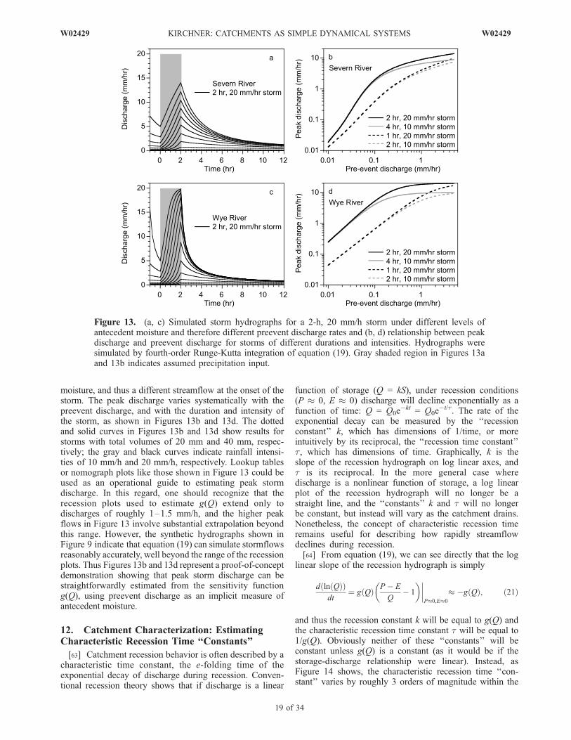
moisture, and thus a different streamflow at the onset of thestorm. The peak discharge varies systematically with thepreevent discharge, and with the duration and intensity ofthe storm, as shown in Figures 13b and 13d. The dottedand solid curves in Figures 13b and 13d show results forstorms with total volumes of 20 mm and 40 mm, respec-tively; the gray and black curves indicate rainfall intensi-ties of 10 mm/h and 20 mm/h, respectively. Lookup tablesor nomograph plots like those shown in Figure 13 could beused as an operational guide to estimating peak stormdischarge. In this regard, one should recognize that therecession plots used to estimate g(Q) extend only todischarges of roughly 1–1.5 mm/h, and the higher peakflows in Figure 13 involve substantial extrapolation beyondthis range. However, the synthetic hydrographs shown inFigure 9 indicate that equation (19) can simulate stormflowsreasonably accurately, well beyond the range of the recessionplots. Thus Figures 13b and 13d represent a proof-of-conceptdemonstration showing that peak storm discharge can bestraightforwardly estimated from the sensitivity functiong(Q), using preevent discharge as an implicit measure ofantecedent moisture.

12. Catchment Characterization: EstimatingCharacteristic Recession Time ‘‘Constants’’

[63] Catchment recession behavior is often described by acharacteristic time constant, the e-folding time of theexponential decay of discharge during recession. Conven-tional recession theory shows that if discharge is a linear

function of storage (Q = kS), under recession conditions(P � 0, E � 0) discharge will decline exponentially as afunction of time: Q = Q0e

�kt = Q0e�t/t. The rate of the

exponential decay can be measured by the ‘‘recessionconstant’’ k, which has dimensions of 1/time, or moreintuitively by its reciprocal, the ‘‘recession time constant’’t, which has dimensions of time. Graphically, k is theslope of the recession hydrograph on log linear axes, andt is its reciprocal. In the more general case wheredischarge is a nonlinear function of storage, a log linearplot of the recession hydrograph will no longer be astraight line, and the ‘‘constants’’ k and t will no longerbe constant, but instead will vary as the catchment drains.Nonetheless, the concept of characteristic recession timeremains useful for describing how rapidly streamflowdeclines during recession.[64] From equation (19), we can see directly that the log

linear slope of the recession hydrograph is simply

d ln Qð Þð Þdt

¼ g Qð Þ P � E

Q� 1

��P�0;E�0

� �g Qð Þ; ð21Þ

and thus the recession constant k will be equal to g(Q) andthe characteristic recession time constant t will be equal to1/g(Q). Obviously neither of these ‘‘constants’’ will beconstant unless g(Q) is a constant (as it would be if thestorage-discharge relationship were linear). Instead, asFigure 14 shows, the characteristic recession time ‘‘con-stant’’ varies by roughly 3 orders of magnitude within the

Figure 13. (a, c) Simulated storm hydrographs for a 2-h, 20 mm/h storm under different levels ofantecedent moisture and therefore different preevent discharge rates and (b, d) relationship between peakdischarge and preevent discharge for storms of different durations and intensities. Hydrographs weresimulated by fourth-order Runge-Kutta integration of equation (19). Gray shaded region in Figures 13aand 13b indicates assumed precipitation input.


19 of 34

W02429

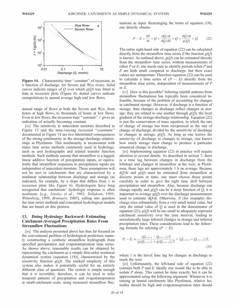
annual range of flows at both the Severn and Wye, fromhours at high flows, to thousands of hours at low flows.Even at low flows, the recession time ‘‘constant’’ t gives noindication of actually becoming constant.[65] The sensitivity to antecedent moisture described in

Figure 13 and the time-varying recession ‘‘constants’’documented in Figure 14 are two interrelated consequencesof the strong nonlinearity in the storage-discharge relation-ships at Plynlimon. This nonlinearity is inconsistent withmany time series methods commonly used in hydrology,such as unit hydrographs and related transfer functionmethods. Such methods assume that streamflow is a lagged,linear additive function of precipitation inputs, or equiva-lently that streamflow responses to precipitation inputs areindependent of antecedent moisture. These assumptions willnot be met in catchments that are characterized by anonlinear relationship between discharge and storage (asindicated, for example, by a slope that differs from 1 inrecession plots like Figure 6). Hydrologists have longrecognized that catchments’ hydrologic response is oftennonlinear, [e.g., Linsley et al., 1982; Tallaksen, 1995;Wittenberg, 1999; Brutsaert, 2005], calling into questionthe time series methods and conceptual hydrological modelsthat are based on this premise.

13. Doing Hydrology Backward: EstimatingCatchment-Averaged Precipitation Rates FromStreamflow Fluctuations

[66] The analysis presented above has thus far focused onthe conventional problem of hydrological prediction, name-ly constructing a synthetic streamflow hydrograph fromspecified precipitation and evapotranspiration time series.As shown above, reasonable results can be obtained byrepresenting the catchment as a simple first-order nonlineardynamical system (equation (18)), characterized by thesensitivity function g(Q). The marked simplicity of thissystem also makes it potentially useful for an entirelydifferent class of questions. The system is simple enoughthat it is invertible; therefore, it can be used to infertemporal patterns of precipitation and evapotranspirationat small-catchment scale, using measured streamflow fluc-

tuations as input. Rearranging the terms of equation (18),one directly obtains

P � E ¼ dS

dtþ Q ¼ dQ=dt

dQ=dSþ Q ¼ dQ=dt

g Qð Þ þ Q: ð22Þ

The entire right-hand side of equation (22) can be calculateddirectly from the streamflow time series if the function g(Q)is known. As outlined above, g(Q) can be estimated directlyfrom the streamflow time series, without measurements ofeither P or E; one needs only to identify periods when P andE are both small compared to discharge, but their exactvalues are unimportant. Therefore equation (22) can be usedto calculate a time series of (P � E) directly from thestreamflow time series, independent of measurements of Por E.[67] How is this possible? Inferring rainfall patterns from

streamflow fluctuations has typically been considered in-feasible, because of the problem of accounting for changesin catchment storage. However, if discharge is a function ofstorage, then changes in discharge reflect changes in stor-age; they are related to one another through g(Q), the localgradient of the storage-discharge relationship. Equation (22)is just the conservation of mass equation, in which the rateof change of storage has been reexpressed as the rate ofchange of discharge, divided by the sensitivity of dischargeto changes in storage, g(Q). As long as one knows thesensitivity of discharge to changes in storage, one knowshow much storage must change to produce a particularmeasured change in discharge.[68] Implementing equation (22) in practice will require

attention to several details. As described in section 7, thereis a time lag between changes in discharge from thehillslope and changes in streamflow at the weir; at Plynli-mon, these lags are approximately 1 h on average. BecausedQ/dt and g(Q) must be estimated from streamflow atdiscrete points in time, one must choose those pointscarefully in order to give the right time shift betweenprecipitation and streamflow. Also, because discharge canchange rapidly and g(Q) can be a steep function of Q, it isimportant to average g(Q) over the discharge measurementsused to estimate dQ/dt. Otherwise, if (for example) dis-charge rises substantially from a very small initial value, butonly the initial value of Q is used in the denominator ofequation (22), g(Q) will be too small to adequately representcatchment sensitivity over the time interval, leading tounrealistically large inferred changes in storage and inferredprecipitation rates. These considerations lead to the follow-ing formula for inferring (P � E):

Pt � Et �Qtþ‘þ1 � Qtþ‘�1ð Þ=2

g Qtþ‘þ1ð Þ þ g Qtþ‘�1ð Þ½ �=2þ Qtþ‘þ1 þ Qtþ‘�1ð Þ=2;

ð23Þ

where ‘ is the travel time lag for changes in discharge toreach the weir.[69] Unfortunately, the left-hand side of equation (22)

contains both P and E. Ideally one would like to be able toisolate P alone. This cannot be done exactly, but it can beapproximated using the following argument. Whenever it israining at humid catchments like Plynlimon, relative hu-midity should be high and evapotranspiration rates should

Figure 14. Characteristic time ‘‘constant’’ of recession, asa function of discharge, for Severn and Wye rivers. Solidcurves indicate ranges of Q over which g(Q) was fitted todata in recession plots (Figure 6); dotted curves indicateextrapolations to annual average high and low flows.

20 of 34


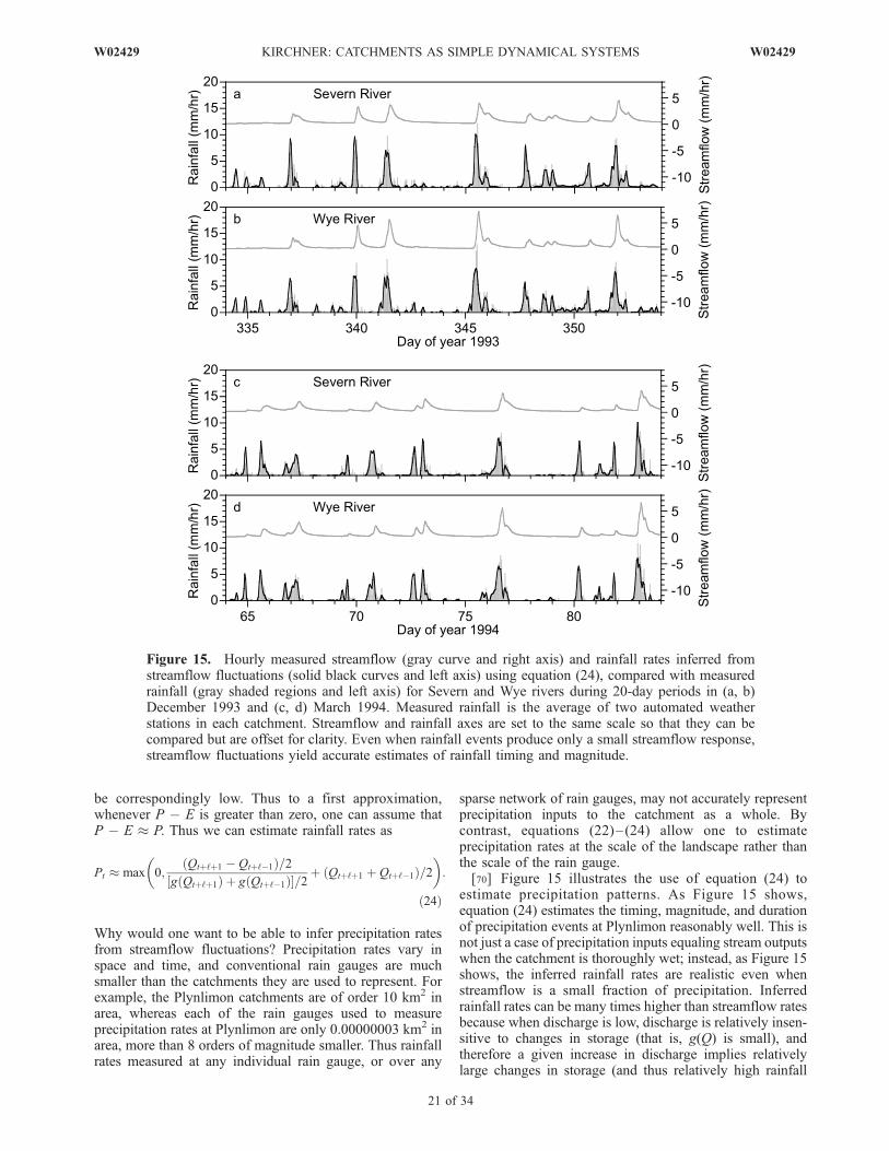
be correspondingly low. Thus to a first approximation,whenever P � E is greater than zero, one can assume thatP � E � P. Thus we can estimate rainfall rates as

Pt � max 0;Qtþ‘þ1 � Qtþ‘�1ð Þ=2

g Qtþ‘þ1ð Þ þ g Qtþ‘�1ð Þ½ �=2þ Qtþ‘þ1 þ Qtþ‘�1ð Þ=2

:

ð24Þ

Why would one want to be able to infer precipitation ratesfrom streamflow fluctuations? Precipitation rates vary inspace and time, and conventional rain gauges are muchsmaller than the catchments they are used to represent. Forexample, the Plynlimon catchments are of order 10 km2 inarea, whereas each of the rain gauges used to measureprecipitation rates at Plynlimon are only 0.00000003 km2 inarea, more than 8 orders of magnitude smaller. Thus rainfallrates measured at any individual rain gauge, or over any

sparse network of rain gauges, may not accurately representprecipitation inputs to the catchment as a whole. Bycontrast, equations (22)– (24) allow one to estimateprecipitation rates at the scale of the landscape rather thanthe scale of the rain gauge.[70] Figure 15 illustrates the use of equation (24) to

estimate precipitation patterns. As Figure 15 shows,equation (24) estimates the timing, magnitude, and durationof precipitation events at Plynlimon reasonably well. This isnot just a case of precipitation inputs equaling stream outputswhen the catchment is thoroughly wet; instead, as Figure 15shows, the inferred rainfall rates are realistic even whenstreamflow is a small fraction of precipitation. Inferredrainfall rates can be many times higher than streamflow ratesbecause when discharge is low, discharge is relatively insen-sitive to changes in storage (that is, g(Q) is small), andtherefore a given increase in discharge implies relativelylarge changes in storage (and thus relatively high rainfall

Figure 15. Hourly measured streamflow (gray curve and right axis) and rainfall rates inferred fromstreamflow fluctuations (solid black curves and left axis) using equation (24), compared with measuredrainfall (gray shaded regions and left axis) for Severn and Wye rivers during 20-day periods in (a, b)December 1993 and (c, d) March 1994. Measured rainfall is the average of two automated weatherstations in each catchment. Streamflow and rainfall axes are set to the same scale so that they can becompared but are offset for clarity. Even when rainfall events produce only a small streamflow response,streamflow fluctuations yield accurate estimates of rainfall timing and magnitude.


21 of 34

W02429

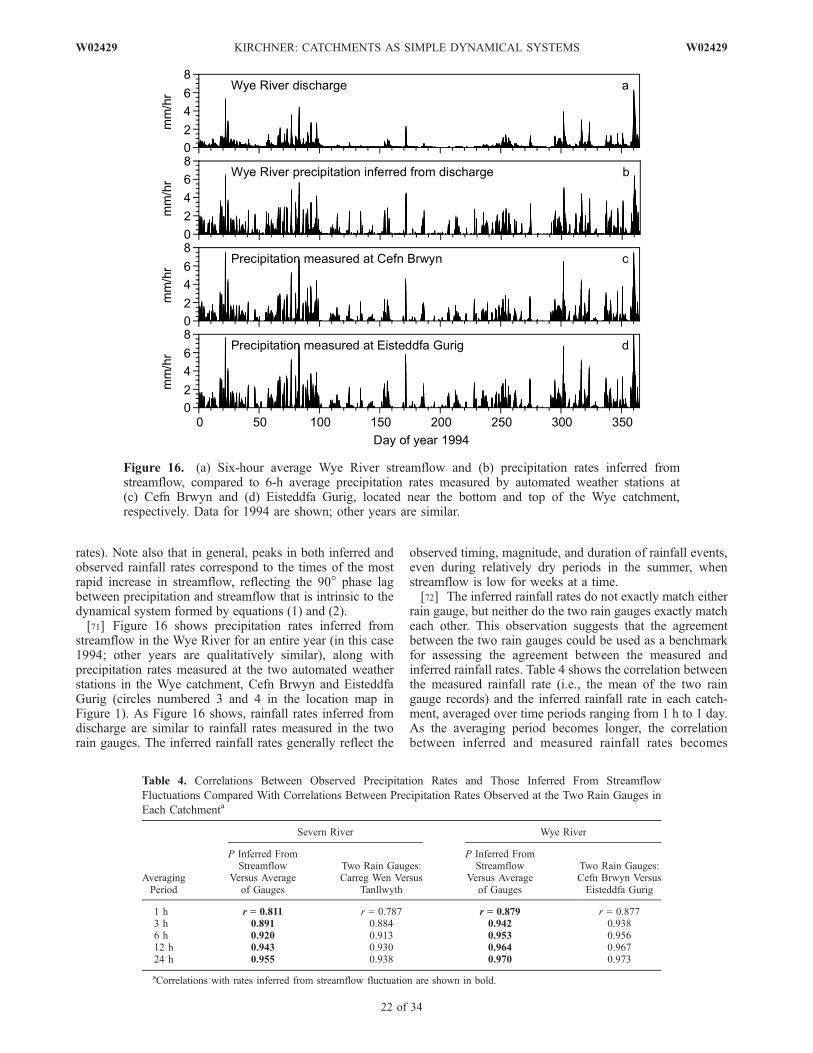
rates). Note also that in general, peaks in both inferred andobserved rainfall rates correspond to the times of the mostrapid increase in streamflow, reflecting the 90� phase lagbetween precipitation and streamflow that is intrinsic to thedynamical system formed by equations (1) and (2).[71] Figure 16 shows precipitation rates inferred from

streamflow in the Wye River for an entire year (in this case1994; other years are qualitatively similar), along withprecipitation rates measured at the two automated weatherstations in the Wye catchment, Cefn Brwyn and EisteddfaGurig (circles numbered 3 and 4 in the location map inFigure 1). As Figure 16 shows, rainfall rates inferred fromdischarge are similar to rainfall rates measured in the tworain gauges. The inferred rainfall rates generally reflect the

observed timing, magnitude, and duration of rainfall events,even during relatively dry periods in the summer, whenstreamflow is low for weeks at a time.[72] The inferred rainfall rates do not exactly match either

rain gauge, but neither do the two rain gauges exactly matcheach other. This observation suggests that the agreementbetween the two rain gauges could be used as a benchmarkfor assessing the agreement between the measured andinferred rainfall rates. Table 4 shows the correlation betweenthe measured rainfall rate (i.e., the mean of the two raingauge records) and the inferred rainfall rate in each catch-ment, averaged over time periods ranging from 1 h to 1 day.As the averaging period becomes longer, the correlationbetween inferred and measured rainfall rates becomes

Figure 16. (a) Six-hour average Wye River streamflow and (b) precipitation rates inferred fromstreamflow, compared to 6-h average precipitation rates measured by automated weather stations at(c) Cefn Brwyn and (d) Eisteddfa Gurig, located near the bottom and top of the Wye catchment,respectively. Data for 1994 are shown; other years are similar.

Table 4. Correlations Between Observed Precipitation Rates and Those Inferred From Streamflow

Fluctuations Compared With Correlations Between Precipitation Rates Observed at the Two Rain Gauges in

Each Catchmenta

AveragingPeriod

Severn River Wye River

P Inferred FromStreamflow

Versus Averageof Gauges

Two Rain Gauges:Carreg Wen Versus

Tanllwyth

P Inferred FromStreamflow

Versus Averageof Gauges

Two Rain Gauges:Cefn Brwyn VersusEisteddfa Gurig

1 h r = 0.811 r = 0.787 r = 0.879 r = 0.8773 h 0.891 0.884 0.942 0.9386 h 0.920 0.913 0.953 0.95612 h 0.943 0.930 0.964 0.96724 h 0.955 0.938 0.970 0.973

aCorrelations with rates inferred from streamflow fluctuation are shown in bold.

22 of 34


stronger, because small discrepancies in timing become lessconsequential. As a benchmark for comparison, Table 4 alsoshows the correlation between the precipitation rates mea-sured at the two rain gauges in each catchment. In general,the correlations between the measured and inferred rainfallrates are similar to the correlations between the two raingauges. In other words, the inferred rainfall rates agree withthe rain gauges roughly as well as the two rain gauges agreewith each other.[73] The comparison between inferred and measured

precipitation rates is a strong test of the underlying theory.Equations (22)–(24) are not calibrated in any way to theprecipitation data that they are tested against, because thesensitivity function g(Q) is estimated from the streamflowtime series alone. Thus Figures 15 and 16 and Table 4 are acompletely independent test of the theory. Furthermore, inan information-theoretic sense, precipitation is a moreinformation-rich time series than streamflow, which issmoother and thus more redundant with itself through time.Therefore the precipitation time series provides a morerichly detailed set of observations for the theory to be testedagainst. The history of hydrology shows that many differentrainfall-runoff models can successfully take an information-rich precipitation time series and smooth it out to make arealistic-looking, information-poor streamflow time series.It is less obvious that this process should be reversible, suchthat subtle fluctuations in the streamflow time series yieldrealistic estimates of precipitation rates through time. It iseven less obvious that this should be possible without anycalibration to the precipitation time series, yet this is whatequations (22)–(24) do.

[74] Because precipitation at Plynlimon is relatively uni-form in space (as indicated by the strong correlationsbetween the pairs of rain gauges), the size of the effective‘‘footprint’’ of the inferred precipitation estimate is unclear;does it encompass the entire catchment, or a more limitedarea adjacent to the stream network? In either case, theeffective footprint of the precipitation estimates is orders ofmagnitude larger than conventional rain gauges, and morewidely distributed across the landscape. Such spatiallyintegrated precipitation estimates are potentially useful for‘‘scaling up’’ individual rain gauge records to the scale ofsmall catchments. Likewise, precipitation time series in-ferred from streamflow may provide useful ‘‘ground truth’’for radar-based precipitation estimates, which have a typicalpixel size on the same order as small catchments (but manyorders of magnitude larger than conventional rain gauges).Precipitation estimates from streamflow may also be usefulin estimating catchment inputs that are difficult to measuredirectly, such as snowmelt, canopy interception, or fog drip.[75] Precipitation estimates derived from streamflow fluc-

tuations may also be useful in reconstructing past precipi-tation, in cases where streamflow records are available butprecipitation records are not. To explore this possibility, Iused hourly streamflow records from 1974 through 2000 toreconstruct hourly precipitation estimates for the two catch-ments over those years, using equation (24). I then aggre-gated these precipitation estimates to annual totals, andcompared them against annual precipitation totals from adense network of monthly read storage rain gauges in thetwo catchments [Marc and Robinson, 2007]. The sensitivityfunctions g(Q) for the two catchments were the same ones

Figure 17. Annual precipitation totals inferred from streamflow fluctuations (black dots) for Severn andWye catchments, compared to annual precipitation captured in a dense network of storage gauges [Marcand Robinson, 2007].


23 of 34

W02429

estimated earlier from the recession plots (Figure 6). AsFigure 17 shows, the inferred precipitation totals agreealmost exactly with the rain gauge measurements in theWye catchment. In the Severn catchment, the inferredprecipitation totals are strongly correlated with the raingauge measurements, but are 150–200 mm/a higher, onaverage. As before, the inferred precipitation estimates arenot calibrated in any way to the rain gauge measurements.Thus the results shown in Figure 17 provide strong supportfor the underlying theory, and suggest that these methodsmay be useful for inferring precipitation rates where directmeasurements are not available.

14. Doing Hydrology Backward: InferringEvapotranspiration Patterns From StreamflowFluctuations

[76] Because streamflow fluctuations quantitatively re-flect precipitation inputs to the catchment, as shown above,it is natural to ask whether streamflow fluctuations alsoreflect evapotranspiration losses. Hydrologists have devel-oped several strategies over the past few decades for usingdischargemeasurements during streamflow recession to infercatchment-scale evapotranspiration rates [e.g., Tschinkel,1963; Daniel, 1976; Brutsaert, 1982; Boronina et al.,2005; Szilagyi et al., 2007]. In the dynamical system de-scribed by equations (1) and (2), precipitation and evapo-transpiration have comparable but opposite effects oncatchment storage and thus on streamflow. This raises thepossibility that streamflow fluctuations can be used to infertemporal patterns of landscape-scale evapotranspiration aswell as precipitation. It is therefore interesting to test how

well streamflow reflects evapotranspiration rates, even atPlynlimon, where evapotranspiration is a relatively smallfraction of the water balance (Table 1).[77] The catchment mass balance can be rewritten to

express the rate of evapotranspiration as

E ¼ P � Q� dS

dt¼ P � Q� dQ=dt

g Qð Þ : ð25Þ

It would appear logical to use equation (25) to estimateevapotranspiration rates directly from measured rainfallrates and streamflow fluctuations. In practice, however, theuncertainty in P during rainfall events will be many timesbigger than E (which is on the order of 0.1 mm/h), makingthe direct application of equation (25) impractical.[78] Instead, the approach adopted here is to restrict the

analysis to rainless periods (defined for Plynlimon asperiods when no precipitation is recorded in any of the fourrain gauges during the previous 6 h or the following 2 h, asin section 5 above). Under those conditions, one can assumethat P, and thus the uncertainty in P, must be small. Then thesame considerations used to derive equation (24) lead to thefollowing expression for inferring evapotranspiration ratesfrom streamflow fluctuations:

EtjP¼0¼ � dQ=dt

g Qð Þ � Q � � Qtþ‘þ1 � Qtþ‘�1ð Þ=2g Qtþ‘þ1ð Þ þ g Qtþ‘�1ð Þ½ �=2

� Qtþ‘þ1 þ Qtþ‘�1ð Þ=2; ð26Þ

where, as in equation (23), ‘ is the travel time lag forchanges in discharge to reach the weir.

Figure 18. (a, c) Fluctuations in Severn and Wye River discharge during an extended rainless interval inJune 1992. (b, d) Evapotranspiration rates inferred from these streamflow fluctuations (black curves) andPenman-Monteith evapotranspiration estimates calculated from automatic weather station data (graycurves). The discharge fluctuations are extremely small; the axes of Figures 18a and 18c are enlarged by afactor of 50 relative to Figures 18b and 18d. Dotted gray lines in Figures 18b and 18d show streamdischarge drawn to scale. Vertical bars mark midnight.

24 of 34


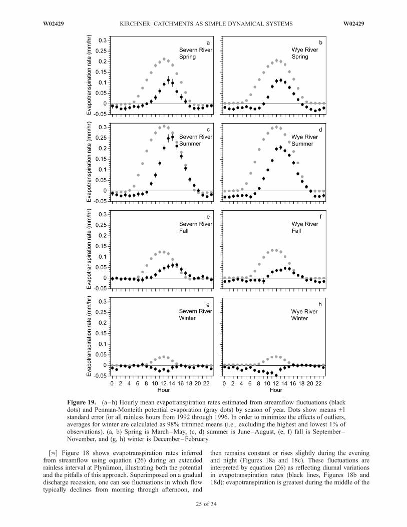
[79] Figure 18 shows evapotranspiration rates inferredfrom streamflow using equation (26) during an extendedrainless interval at Plynlimon, illustrating both the potentialand the pitfalls of this approach. Superimposed on a gradualdischarge recession, one can see fluctuations in which flowtypically declines from morning through afternoon, and

then remains constant or rises slightly during the eveningand night (Figures 18a and 18c). These fluctuations areinterpreted by equation (26) as reflecting diurnal variationsin evapotranspiration rates (black lines, Figures 18b and18d): evapotranspiration is greatest during the middle of the

Figure 19. (a–h) Hourly mean evapotranspiration rates estimated from streamflow fluctuations (blackdots) and Penman-Monteith potential evaporation (gray dots) by season of year. Dots show means ±1standard error for all rainless hours from 1992 through 1996. In order to minimize the effects of outliers,averages for winter are calculated as 98% trimmed means (i.e., excluding the highest and lowest 1% ofobservations). (a, b) Spring is March–May, (c, d) summer is June–August, (e, f) fall is September–November, and (g, h) winter is December–February.


25 of 34

W02429

day, leading to a decline in catchment storage and acorresponding reduction in streamflow.[80] However, the discharge measurements must be very

precise or else the discharge fluctuations will be obscuredby measurement noise, because the fluctuations in dischargeare tiny. In fact, to make the discharge fluctuations visible inFigure 18, the discharge axes have been expanded byfiftyfold relative to the evapotranspiration plots. The dis-charge time series are shown to scale as the gray dotted linesin Figure 18b and 18d; on that scale, the discharge fluctua-tions are invisible. Because discharge is low, the catchmentsensitivity function g(Q) is small as well, reflecting the factthat when the catchment is dry, discharge is relativelyinsensitive to changes in storage. Thus small changes indischarge imply large changes in storage; in equation (26),this has the effect of amplifying the real fluctuations indischarge, but also amplifying the measurement noise. As aresult, the inferred diurnal cycles of evapotranspiration arenoisy. Nonetheless, they roughly agree with the magnitudeand timing of the diurnal cycles in Penman-Monteith poten-tial evaporation, shown as the gray lines in Figures 18b and18d.[81] Reducing the noise in the inferred evapotranspiration

rates would require measuring subtle streamflow fluctua-tions very accurately, which the Plynlimon stream gaugingstations were not designed to do. Given the noisy data thatare available, however, one can still clarify the diurnalpatterns in evapotranspiration by averaging over many dailycycles. Figure 19 shows the inferred evapotranspirationrates for each hour of the day in each season, averagedover all rainless hours from 1992 through 1996. Thecorresponding cycles in Penman-Monteith potential evapo-ration are shown in gray for comparison. As Figure 19shows, the evapotranspiration cycles inferred from stream-flow fluctuations are broadly consistent with the Penman-Monteith estimates, although both the timing and amplitudediffer somewhat. It should be kept in mind that the Penman-Monteith estimates of potential evaporation are not them-selves a ‘‘gold standard,’’ because it is not clear how theyshould be extrapolated to the scale of the landscape.Nonetheless, both the Penman-Monteith estimates and theinferred evapotranspiration rates reach their peak near themiddle of the day and fall to near zero at night. Predictedand observed diurnal cycles vary similarly from one seasonto the next, with the exception of the winter, when theinferred evapotranspiration cycle is weak but appears to beinverted from the Penman-Monteith estimates. That is, onaverage there appears to be a small input of water to thecatchment near noon; this could potentially reflect meltingof frost or snow during the middle of the day.[82] The strongest conclusion one can draw from

Figures 18 and 19 is that equation (26) provides at leastsemiquantitative estimates of evapotranspiration rates.Nonetheless, the fact that this works at all, even at Plynli-mon where evapotranspiration rates are relatively low anddischarge fluctuations are correspondingly tiny, represents astrong test of the dynamical systems approach developedhere. It is important to remember that the only parameters inequation (26) are those embedded in the sensitivity functiong(Q), and that g(Q) is estimated from recession plots thatcontain no information about evapotranspiration rates.Therefore evapotranspiration estimates like those shown in

Figure 18 and 19 are not calibrated to observed evapotrans-piration rates in any way, and thus represent a completelyindependent test of the theory.[83] Even in the most general qualitative sense, one sees

the signature of the dynamical system in temporal patternsshown in Figure 18. One can see that in general, there is a90� phase lag between the variations in evapotranspirationrates and the fluctuations in streamflow. Because evapo-transpiration depletes catchment storage, which in turnregulates discharge to the stream, the midday peak inevapotranspiration rates corresponds to the fastest declinein streamflow (not the minimum streamflow, as it would ifevapotranspiration were removing water directly from thestream). This is the same dynamical phase lag that wasnoted in sections 3 and 13 between precipitation andstreamflow.[84] Estimated evapotranspiration rates are determined by

the balance between the two terms of equation (26), whichhave opposite signs during streamflow recession. Becausethe sensitivity function g(Q) determines the balance be-tween the two terms in equation (26), inaccuracies inestimating g(Q) could have large effects on evapotranspi-ration rates inferred from streamflow. However, even incases where equation (26) does not give quantitativelyaccurate estimates of absolute rates, it may still be usefulin estimating relative changes in evapotranspiration ratesthrough time. Estimates of changes in evapotranspiration

Figure 20. Difference between annual evapotranspirationrates in the Severn and Wye catchments, inferred fromstreamflow fluctuations (black dots with standard errors), andfrom mass balances (gray curve). Mass balances werecalculated from precipitation recorded in an extensivenetwork of monthly read storage rain gauges and fromstreamflows at the Severn flume and Wye weir (data fromMarc and Robinson [2007]). Black dots are trimmed meansof hourly evapotranspiration rates (upper and lower 1% ofdata excluded to minimize the effect of outliers), calculatedfrom streamflow fluctuations using equation (26) duringrainless periods (defined as zero rainfall recorded at allautomated weather stations from the previous 6 h through thefollowing 2 h; periods with fewer than two operationalweather stations were excluded). Inferred evapotranspirationrates were averaged for each season and thenwere aggregatedto annual time scales; standard errors were calculated by first-order, second-moment error propagation.

26 of 34


rates over time may be useful for assessing the effects ofchanges in climate or land use on the water cycle. Forexample, concerns over the hydrologic effects of changes invegetation (particularly afforestation of moorland areas)were the original motivation for long-term research atPlynlimon. Painstaking water balance studies, based onnetworks of dozens of storage-type rain gauges that wereread monthly, have shown that during the 1970s and 1980s,transpiration rates in the forested catchment (Severn) weresomewhat higher than in the moorland catchment (Wye).However, over time the difference in evapotranspirationrates between the two catchments has decreased becauseof both the increasing age of the forest stand and the gradualreduction of the forested area through timber harvesting[Robinson and Dupeyrat, 2005; Marc and Robinson, 2007].[85] To test whether this change in evapotranspiration

rates could also be detected from streamflow fluctuations, Iapplied equation (26) to the hourly discharge records fromthe Severn and Wye rivers over the 26 years from 1975through 2000. This analysis used the same g(Q) functionsused elsewhere in this paper, estimated from the recessionplots in Figure 6. As Figure 20 shows, the fluctuations instreamflow in the two catchments indicate a gradual declinein evapotranspiration rates in the Severn relative to the Wyethrough the 1970s and 1980s, reproducing the general trendobserved in the mass balance studies at Plynlimon over thesame period (gray line, Figure 20). It bears emphasis thatthe inferred evapotranspiration rates shown in Figure 20 arenot calibrated in any way to either Penman-Monteithestimates or to catchment mass balances. Indeed, the aver-age evapotranspiration rates inferred from streamflow fluc-tuations in both of the catchments are low, on average,compared to either Penman-Monteith or mass balanceestimates. This could arise because equation (26) omitsinterception losses, which are included in evapotranspira-tion rates inferred from catchment mass balances. It couldalso arise if g(Q) is somewhat too high at low flows, leadingto a persistent bias in the relative sizes of the two terms ofequation (26). Nonetheless, equation (26) reproduces thedifference in evapotranspiration rates between the twocatchments, and the trend in that difference through time(Figure 20), suggesting that this approach may be useful fordetecting how landscape-scale evapotranspiration rates re-spond to changes in vegetation or climate.

15. Discussion

15.1. Comparison With Previous Analyses

[86] In the long history of recession analysis in hydrolo-gy, there have been many attempts to relate the recessionbehavior of streams to a catchment-scale drainage function;see reviews by Hall [1968], Tallaksen [1995], and Smakhtin[2001], and references therein, as well as more recent workby Lamb and Beven [1997], Wittenberg and Sivapalan[1999], Wittenberg [1999, 2003], Szilagyi et al. [2007],and Rupp and Woods [2008]. The approach presented herediffers from each of these previous efforts in one or more ofthe following four ways. First, in the present approach thestorage-discharge relationship is expressed in its implicitdifferential form, the sensitivity function g(Q). This isadvantageous because g(Q) can be estimated directly fromrecession plots such as Figure 6, and because it allows the

dynamical system to be expressed as a single first-orderdifferential equation. This equation is invertible, allowingone to estimate precipitation or evapotranspiration from thestreamflow time series, as well as to predict the hydrographfrom precipitation and evapotranspiration time series.[87] Second, the present approach does not specify the

form of the relationship between storage and discharge, orthe corresponding sensitivity function g(Q), instead allow-ing it to be determined directly from streamflow data. Thismakes the analysis more general and portable than one thatassumes that the storage-discharge relationship must have aparticular functional form. In this respect the approach is anot a ‘‘black box’’ model, but rather a ‘‘gray box’’ systemsanalysis tool (in the sense of Kirchner [2006]) because ituses the catchment’s behavior to reveal what its governingequations are. Because the sensitivity function is determineddirectly from streamflow data and encapsulates the drainagebehavior of the catchment in concise form, it may also be auseful tool for catchment characterization.[88] Third, the present approach attempts, as much as

possible, to take account of the uncertainties and confound-ing factors that typically affect catchment data. As Tallaksen[1995] points out, many recession analyses (but see Lamband Beven [1997] for an exception) pay too little attention tothe confounding effects of evapotranspiration, even thoughits potential to significantly steepen recession curves hasbeen known for decades [e.g., Federer, 1973]. The reces-sion plots used to estimate g(Q), by contrast, do not requirecontinuous recession curves, so one can filter out data thatare significantly affected by evapotranspiration. Similarly,the bounding lines that are typically fitted to recession plotsof the Brutsaert-Nieber type [Brutsaert and Nieber, 1977]are susceptible to biases and artifacts [Rupp and Selker,2006a], which the curve-fitting procedure in Figure 6 isdesigned to avoid.[89] Fourth, the present approach makes no distinction

between base flow and quick flow. Instead, it treats catch-ment drainage, from base flow to peak stormflow and backagain, as a single continuum of hydrological behavior. Thiseliminates the need to separate the hydrograph into differentcomponents, and makes the analysis simple, general andportable.

15.2. Model Simplicity and Real-World Complexity

[90] The analysis presented here is based on a very simplemodel structure, but the flow paths and processes control-ling runoff in real-world catchments are complex andspatially heterogeneous. Decades of field observations tes-tify to the complexity of Plynlimon’s flow systems [e.g.,Neal, 2004; Shand et al., 2005]. For example, abundantephemeral springs and soil pipes at Plynlimon indicate aspatially heterogeneous and temporally dynamic flow sys-tem in the subsurface [e.g., Sklash et al., 1996]. Boreholemeasurements on a hillslope in the Severn catchment havealso identified multiple subsurface flow paths and complexinteractions between them, with stormflows creatingdownwelling and upwelling hydraulic gradients in adjacentborehole nests separated by only a few meters [Haria andShand, 2004, 2006]. Thus the Plynlimon catchments arecharacterized by both spatial complexity and process het-erogeneity. Yet at the scale of several square kilometers,these complexities and heterogeneities aggregate to a simple(albeit nonlinear) catchment-scale storage-discharge rela-


27 of 34

W02429

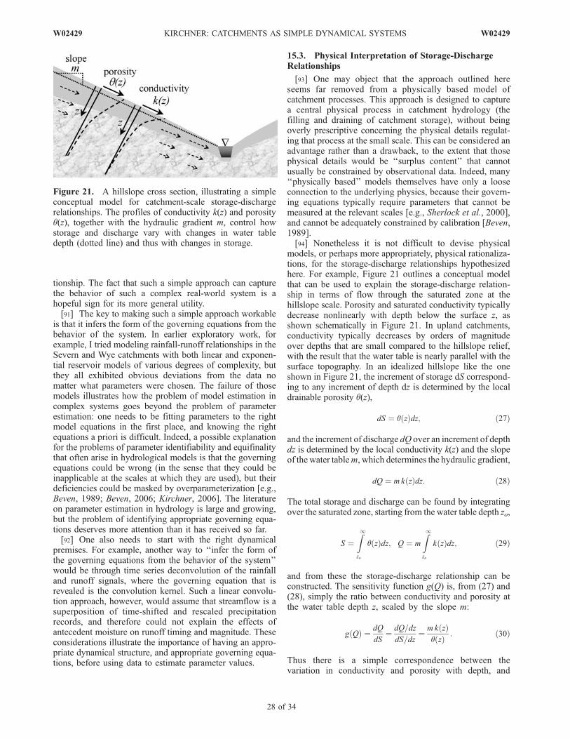
tionship. The fact that such a simple approach can capturethe behavior of such a complex real-world system is ahopeful sign for its more general utility.[91] The key to making such a simple approach workable

is that it infers the form of the governing equations from thebehavior of the system. In earlier exploratory work, forexample, I tried modeling rainfall-runoff relationships in theSevern and Wye catchments with both linear and exponen-tial reservoir models of various degrees of complexity, butthey all exhibited obvious deviations from the data nomatter what parameters were chosen. The failure of thosemodels illustrates how the problem of model estimation incomplex systems goes beyond the problem of parameterestimation: one needs to be fitting parameters to the rightmodel equations in the first place, and knowing the rightequations a priori is difficult. Indeed, a possible explanationfor the problems of parameter identifiability and equifinalitythat often arise in hydrological models is that the governingequations could be wrong (in the sense that they could beinapplicable at the scales at which they are used), but theirdeficiencies could be masked by overparameterization [e.g.,Beven, 1989; Beven, 2006; Kirchner, 2006]. The literatureon parameter estimation in hydrology is large and growing,but the problem of identifying appropriate governing equa-tions deserves more attention than it has received so far.[92] One also needs to start with the right dynamical

premises. For example, another way to ‘‘infer the form ofthe governing equations from the behavior of the system’’would be through time series deconvolution of the rainfalland runoff signals, where the governing equation that isrevealed is the convolution kernel. Such a linear convolu-tion approach, however, would assume that streamflow is asuperposition of time-shifted and rescaled precipitationrecords, and therefore could not explain the effects ofantecedent moisture on runoff timing and magnitude. Theseconsiderations illustrate the importance of having an appro-priate dynamical structure, and appropriate governing equa-tions, before using data to estimate parameter values.

15.3. Physical Interpretation of Storage-DischargeRelationships

[93] One may object that the approach outlined hereseems far removed from a physically based model ofcatchment processes. This approach is designed to capturea central physical process in catchment hydrology (thefilling and draining of catchment storage), without beingoverly prescriptive concerning the physical details regulat-ing that process at the small scale. This can be considered anadvantage rather than a drawback, to the extent that thosephysical details would be ‘‘surplus content’’ that cannotusually be constrained by observational data. Indeed, many‘‘physically based’’ models themselves have only a looseconnection to the underlying physics, because their govern-ing equations typically require parameters that cannot bemeasured at the relevant scales [e.g., Sherlock et al., 2000],and cannot be adequately constrained by calibration [Beven,1989].[94] Nonetheless it is not difficult to devise physical

models, or perhaps more appropriately, physical rationaliza-tions, for the storage-discharge relationships hypothesizedhere. For example, Figure 21 outlines a conceptual modelthat can be used to explain the storage-discharge relation-ship in terms of flow through the saturated zone at thehillslope scale. Porosity and saturated conductivity typicallydecrease nonlinearly with depth below the surface z, asshown schematically in Figure 21. In upland catchments,conductivity typically decreases by orders of magnitudeover depths that are small compared to the hillslope relief,with the result that the water table is nearly parallel with thesurface topography. In an idealized hillslope like the oneshown in Figure 21, the increment of storage dS correspond-ing to any increment of depth dz is determined by the localdrainable porosity q(z),

dS ¼ q zð Þdz; ð27Þ

and the increment of discharge dQ over an increment of depthdz is determined by the local conductivity k(z) and the slopeof the water tablem, which determines the hydraulic gradient,

dQ ¼ mk zð Þdz: ð28Þ

The total storage and discharge can be found by integratingover the saturated zone, starting from the water table depth zo,

S ¼Z1zo

q zð Þdz; Q ¼ m

Z1zo

k zð Þdz; ð29Þ

and from these the storage-discharge relationship can beconstructed. The sensitivity function g(Q) is, from (27) and(28), simply the ratio between conductivity and porosity atthe water table depth z, scaled by the slope m:

g Qð Þ ¼ dQ

dS¼ dQ=dz

dS=dz¼ mk zð Þ

q zð Þ : ð30Þ

Thus there is a simple correspondence between thevariation in conductivity and porosity with depth, and

Figure 21. A hillslope cross section, illustrating a simpleconceptual model for catchment-scale storage-dischargerelationships. The profiles of conductivity k(z) and porosityq(z), together with the hydraulic gradient m, control howstorage and discharge vary with changes in water tabledepth (dotted line) and thus with changes in storage.

28 of 34


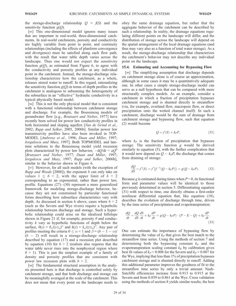
the storage-discharge relationship Q = f(S) and thesensitivity function g(Q).[95] This one-dimensional model ignores many issues

that are important in real-world, three-dimensional catch-ments. In real-world catchments, porosity and conductivityare highly variable from point to point, and continuityrelationships (including the effects of planform convergenceand divergence) must be satisfied along each flow path,with the result that water table depth varies across thelandscape. Thus one would not expect the sensitivityfunction g(Q), as estimated from Figure 6, to agree withthe conductivity and porosity profiles at any individualpoint in the catchment. Instead, the storage-discharge rela-tionship characterizes how the catchment, as a whole,releases stored water to runoff. In this regard, rationalizingthe sensitivity function g(Q) in terms of depth profiles in thecatchment is analogous to subsuming the heterogeneity ofthe subsurface in an ‘‘effective’’ hydraulic conductivity in atypical physically based model.[96] This is not the only physical model that is consistent

with a functional relationship between catchment storageand discharge. For example, the Boussinesq models ofgroundwater flow [e.g., Brutsaert and Nieber, 1977] haverecently been solved for power law conductivity profiles inboth horizontal and sloping aquifers [Van de Grind et al.,2002; Rupp and Selker, 2005, 2006b]. Similar power lawtransmissivity profiles have also been invoked in TOP-MODEL [Ambrose et al., 1996; Duan and Miller, 1997;Iorgulescu and Musy, 1997]. Both TOPMODEL and late-time solutions to the Boussinesq model yield recessionplots characterized by power law behavior, �dQ/dt = aQb

[Brutsaert and Nieber, 1977; Duan and Miller, 1997;Iorgulescu and Musy, 1997; Rupp and Selker, 2006b],similar to the behavior shown in Figure 6.[97] However, for all such models (with the exception of

Rupp and Woods [2008]), the exponent b can only take onvalues 1 � b < 2, with the upper limit of b = 2corresponding to an exponential, rather than power law,profile. Equations (27)–(30) represent a more generalizedframework for modeling storage-discharge behavior, be-cause they are not constrained by particular functionalforms describing how subsurface characteristics vary withdepth. As discussed in section 6 above, cases where b > 2(such as the Severn and Wye rivers) require a hyperbolicrelationship between discharge and storage. Such a hyper-bolic relationship could arise on the idealized hillslopeshown in Figure 21 if, for example, porosity q and conduc-tivity k vary as hyperbolic functions of depth below thesurface, q(z) = qo/(z/zo)

a and k(z) = ko/(z/zo)b. Any pair of

profiles meeting the criteria 0 � a < 1 and b = (b � 1 � a)/(b � 2) will result in a storage-discharge relationshipdescribed by equation (17) and a recession plot describedby equation (10) for b > 2 (realism also requires that thewater table never rises into the nonphysical region whereq > 1). This is just the simplest example of a family ofdensity and porosity profiles that are consistent withpower law recession plots with b > 2.[98] The fundamental structural assumption in the analy-

sis presented here is that discharge is controlled solely bycatchment storage, and that both discharge and storage canbe meaningfully averaged at the scale of the catchment. Thisdoes not mean that every point on the landscape needs to

obey the same drainage equation, but rather that theaggregate behavior of the catchment can be described bysuch a relationship. In reality, the drainage equations regu-lating different points on the landscape will differ, and thedistribution of storage across the landscape will depend onthe spatial arrangement of the local drainage equations (andthus may vary also as a function of total water storage). As aresult, the storage-discharge relationship that characterizesthe catchment’s behavior may not describe any individualpoint on the landscape.

15.4. Estimating and Accounting for Bypassing Flow

[99] The simplifying assumption that discharge dependson catchment storage alone is of course an approximation,although in some cases it may be a quantitatively adequateone. In other cases a simple storage-discharge model canserve as a null hypothesis that can be compared with morestructurally complex models. As an example, consider acatchment in which a fraction of precipitation bypassescatchment storage and is shunted directly to streamflow(via, for example, overland flow, macropore flow, or directprecipitation onto the wetted channel itself). In such acatchment, discharge would be the sum of drainage fromcatchment storage and bypassing flow, such that equation(2) would become

Q ¼ f Sð Þ þ kPP; ð31Þ

where kP is the fraction of precipitation that bypassesstorage. The sensitivity function g would be derivedsimilarly to equation (5), with the further complication thatit would now depend on Q � kPP, the discharge that comesfrom draining of storage:

dQ

dS¼ f 0 Sð Þ ¼ f 0 f �1 Q� kPPð Þ

� �¼ g Q� kPPð Þ: ð32Þ

Because g is estimated during times whenP= 0, its functionalform and parameter values will be identical to thosepreviously determined in section 5. Differentiating equation(31) with respect to time, one directly obtains a first-ordernonlinear differential equation that, like equation (18),describes the evolution of discharge through time, drivenby the time series of precipitation and evapotranspiration:

dQ

dt¼ dQ

dS

dS

dtþ kP

dP

dt¼ g Q� kPPð Þ P � E � Qð Þ þ kP

dP

dt:

ð33Þ

One can estimate the importance of bypassing flow bydetermining the value of kP that gives the best match to thestreamflow time series. Using the methods of section 7 anddetermining both the bypassing constant kP and theevapotranspiration scaling constant kE by calibration givesbest fit values of kP = 0.008 for the Severn and kP = 0.007 fortheWye, implying that less than 1% of precipitation bypassescatchment storage and is shunted directly to runoff. Addingthis additional parameter improves the goodness of fit to thestreamflow time series by only a trivial amount: Nash-Sutcliffe efficiencies increase from 0.913 to 0.915 at theSevern and from 0.859 to 0.861 at the Wye. Cross validationusing the methods of section 8 yields similar results; the best


29 of 34

W02429

fit values of kP are small across all individual years, rangingfrom 0.006 to 0.010 at the Severn and from 0.005 to 0.016 atthe Wye. If the parameters that describe g(Q � kPP) are alsoestimated by calibration, as in section 9, the best fit values ofkP are similarly small (ranging from 0.003 to 0.008 at theSevern and from 0.009 to 0.014 at the Wye), and adding thebypassing term alters the other parameter values by only afew percent or less.[100] These results imply that bypassing flow makes only

a small contribution to streamflow at Plynlimon, and thataccounting for bypassing flow improves streamflow pre-dictions only marginally. Adding this second runoff mech-anism, however, substantially complicates the process ofinferring precipitation patterns from the streamflow timeseries. Because equation (33) depends on both precipitationand its derivative, the simple methods of section 13 do notapply. However, adding this runoff mechanism does notcomplicate efforts to infer evapotranspiration rates fromstreamflow fluctuations, because (as outlined in section 14)those inferences are drawn when precipitation rates (and thusalso their derivatives) are zero.

15.5. Data Requirements

[101] Any analysis is only as good as the data it is based on.It would therefore be useful to systematically assess howbiases and uncertainties in discharge and weather measure-ments might affect the results of this approach, using syn-thetic data. Such a detailed assessment must await a futurepaper, however, as it is beyond the scope of this one.[102] The analysis presented above has used hourly dis-

charge measurements to estimate the sensitivity functiong(Q) for the Severn and Wye rivers, excluding periods thatwere likely to be affected by rainfall or evapotranspiration.One can naturally ask whether the approach developed herecan be used with the daily discharge data that are widelyavailable online. At Plynlimon, hourly discharge and weatherdata have been used primarily because they permit relativelystrict tests of the theory, but nothing in themathematics of thisapproach fundamentally requires the use of any particulartime step. As a test, I reestimated g(Q), following the methodsof section 5, with daily average discharges for the Severn andWye rivers. I included only days for which precipitation andpotential evapotranspiration were less than 10% of discharge,consistent with the criteria outlined in section 5. At Plynli-mon, these criteria are met for only about 60 days in the5 years of record. Nonetheless, the resulting g(Q) functionsyield predictions of (hourly) discharge, and inferences ofhourly precipitation from discharge fluctuations, that aresimilar to those presented in sections 8 and 13, with Nash-Sutcliffe efficiencies typically differing by less than 0.02from those reported in the last column of Table 2, andcorrelations differing by less than 0.02 from those reportedin the bold columns of Table 4.[103] It is important, however, to exclude the effects of

precipitation and evapotranspiration as much as possiblefrom the discharge data used to estimate g(Q). To test whatcould happen if this is not done, I reestimated g(Q) from thehourly discharge data without excluding periods with highpotential evapotranspiration, excluding only periods withrecent rainfall. High evapotranspiration can be expected tolead to steeper streamflow recessions, and thus highervalues of �dQ/dt in recession plots such as Figure 6; thisdistortion will be largest at small values of Q and �dQ/dt.

As a result, the recession plots for the Severn and Wye areless steep, and more upward curving, if periods of highpotential evapotranspiration are not excluded. The predictedstreamflow time series and inferred precipitation rates aredistorted as well, with Nash-Sutcliffe efficiencies that aretypically about 0.1 lower than those shown in Table 2, andcorrelations with observed rainfall up to 0.06 lower thanthose shown in Table 4. These distortions would likely belarger at less humid catchments, where evapotranspiration isa bigger part of the water balance.

15.6. Limitations

[104] The structural simplicity of the approach outlinedhere obviously limits its generality. For example, it cannotbe expected to give reasonable results in a catchment whereHortonian overland flow is a dominant runoff mechanism,without the addition of a bypassing mechanism like the oneproposed above. Nonetheless, the methods outlined abovecan be used to test whether bypassing flow is important, andit is likely that there are many catchments where bypassingflow is only a small component of runoff.[105] In snowmelt-dominated catchments, liquid water

storage (and thus discharge) will respond to the rate ofsnowmelt rather than the rate of precipitation (i.e., snowfall)per se. Thus the ‘‘precipitation’’ rate inferred from stream-flow fluctuations using the methods of section 13 willrepresent the rate of snowmelt and liquid precipitationreaching the ground surface. The fact that streamflowfluctuations reflect snowmelt rather than snowfall shouldperhaps be considered an advantage rather than a drawback,because this is one of the only methods by which spatiallyaveraged snowmelt rates can be estimated.[106] A bigger challenge is presented by catchments in

which runoff is controlled by interconnected subsurfacereservoirs with different storage-discharge relationships. Insome catchments, for example, streamflow rises and falls ina daily oscillation driven by diurnal evapotranspirationcycles [Lundquist and Cayan, 2002; Czikowsky andFitzjarrald, 2004]. Such behavior cannot be explainedby a single reservoir with a single storage-dischargerelationship, in which evapotranspiration losses shouldproduce daily reductions in streamflow and discharge,but no rebound at night. Instead, a daily oscillation instreamflow would seem to imply a riparian zone that iscontinually recharged by drainage from upslope, withevapotranspiration losses leading to net declines in stor-age (and thus streamflow) during the day, and rechargefrom upslope leading to net increases in storage (and thusstreamflow) at night. The challenge in any such multi-component system is that one cannot easily infer theproperties of any individual component from the behaviorof the system as a whole (as with the simple methodsdeveloped here).[107] The methods outlined here also cannot be applied to

ephemeral streams, because when discharge goes to zero,different levels of storage will correspond to the same (i.e.,zero) discharge. Thus f(S) will be noninvertible and g(Q)will be ill defined. This sets a practical lower limit to thesize of catchments where these methods can be applied,since they must be large enough to support permanentstreams.[108] It is equally clear that these methods must break

down for catchments that are too large, but it is not yet clear

30 of 34


how big is too big. The catchments studied here are roughly10 km2 in area. One can speculate that in significantly largercatchments (say, 1000 km2 in area), the lag times requiredfor changes in discharge to propagate through the channelnetwork would be so long, and so variable with distancefrom the outlet, that the methods presented here would notwork. Also, if storage-discharge relationships are spatiallyheterogeneous at all scales, the methods presented herecannot be expected to work in catchments that are muchlarger than individual storm systems. In such a catchment,the runoff response to an individual storm will depend onthe storage-discharge relationship and antecedent moisturein whatever part of the catchment the storm lands. Thus theapparent storage-discharge relationship, as viewed from thecatchment outlet, could vary significantly from one storm tothe next.[109] By contrast, in catchments that are smaller than the

scale of individual storms, each storm will typically cover thewhole catchment area. For the reasons outlined earlier in thissection, one would expect the aggregation of spatial hetero-geneity in such a catchment to be repeatable from one stormto the next, yielding a catchment-scale storage-dischargerelationship that is stable through time. Similar results wouldbe obtained even in catchments that are larger than individualstorms, if the local storage-discharge relationships are spa-tially heterogeneous on small scales, but relatively uniform,on average, at the scale of individual storms.[110] In large river basins, rainfall-runoff behavior is

determined more by the spatial distribution of precipitationand the routing of flood flows through the channel network,and less by the storage-discharge dynamics considered here.However, the approach presented here may still be helpfulin large basins, by providing a small-catchment runoff‘‘kernel’’ that can be aggregated through the channel net-work. Linking this dynamical systems approach with chan-nel routing via a geomorphic instantaneous unit hydrograph(or similar approach) could help in understanding both thenonlinear response and travel time delays that characterizethe hydrologic behavior of large basins.[111] These considerations highlight the importance of

understanding how storage-discharge relationships varyacross the landscape. Much could be learned by using themethods outlined here to measure g(Q) across nested net-works of small gauged catchments. Work on this is currentlyunderway.[112] Because g(Q) captures the integrated drainage be-

havior of catchments (at least those that are well approximat-ed by the simple structural assumptions envisioned here), itmay provide a useful framework for catchment characteriza-tion. Little is known yet about how consistent g(Q) is fromone catchment to the next, or how much (and how system-atically) it varies with a catchment’s near-surface geology, itssoil characteristics, its geomorphic properties, its climaticsetting, and so forth. Tague and Grant [2004], however, haveshown that the log-log slope and intercept of recession plots forstreams in the Cascade Mountains of Oregon are correlatedwith the fraction of highly conductive Plio-Pleistocene vol-canic bedrock in their catchments. If g(Q) can be estimatedfrom some combination of catchment characteristics, thenit may help in solving the problem of hydrologic predictionin ungauged basins. If, on the other hand, g(Q) cannot beestimated reliably from catchment characteristics, it may

imply that catchments’ storage-discharge behavior dependson catchment properties that cannot be readily measured(such as, for example, the variation in hydraulic conductivitywith depth) and thus that the ungauged basins problem cannotbe solved. In that case, the most efficient way forward may beto simply gauge catchments long enough to estimate theirsensitivity functions g(Q), as an implicit measure of thehidden catchment properties that control their fundamentalhydrologic behavior.

16. Summary and Conclusions

[113] In catchments where discharge Q is a function ofstorage S, the storage-discharge relationship Q = f(S) can becombined with the conservation-of-mass equation to form anonlinear first-order dynamical system (equations (1) and(2)). This dynamical system becomes particularly simple ifthe storage-discharge relationship is expressed in its implicitdifferential form, the hydrologic sensitivity function g(Q) =dQ/dS (equation (5)). Both the mathematical form and theparameters of this sensitivity function can be estimateddirectly from recession plots (Figure 6) showing how therate of streamflow recession �dQ/dt varies with dischargeQ, under conditions where precipitation and evapotranspi-ration rates are negligible compared to discharge.[114] Using the sensitivity function g(Q), the relationship

between precipitation, evapotranspiration, and runoffthrough time can be encapsulated in a single first-ordernonlinear ordinary differential equation (equation (18)).This equation can be numerically integrated to straightfor-wardly model rainfall-runoff behavior through time (Figures9 and 10). The performance of this single-equation rainfall-runoff model, as measured by its Nash-Sutcliffe efficiency,is similar to models that are much more complex and muchmore highly parameterized. Estimating the model parame-ters using different years of data, whether via recession plotsor via direct parameter calibration, yields consistent param-eter values and consistently high model performance(Tables 2 and 3). The consistency of parameter values andmodel performance across different years with differentweather conditions indicates that this approach meets acrucial criterion of mathematical modeling: the constantsstay constant while the variables vary. Cross-validation testsshow that model performance is similar when tested againstyears that were used for parameter estimation, and years thatwere not (Tables 2 and 3), indicating that the model is morethan just a mathematical marionette that can only ‘‘dance’’to the tune of its own calibration data.[115] The sensitivity function g(Q) is a useful tool for

catchment characterization. From g(Q), one can directlyestimate a catchment’s dynamic storage (section 10), itssensitivity to antecedent moisture (section 11), and itsrecession time constants (section 12). More generally,because g(Q) compactly summarizes how catchments storeand release water, it may provide a tool for linking hydro-logic behavior to measurable catchment characteristics.[116] Because the dynamical system that links precipita-

tion, evapotranspiration, runoff, and storage can beexpressed in a single ordinary differential equation, it canalso be inverted, to express the balance between precipita-tion and evapotranspiration as a function only of dischargeand its time derivative (equation (22)). Thus one can usestreamflow fluctuations to estimate time series of spatially


31 of 34

W02429

averaged precipitation and evapotranspiration. Precipitationtime series inferred from streamflow accurately reproducethe timing, duration, and intensity of rainfall events ob-served at Plynlimon (Figures 15 and 16), as well as long-term variations in annual rainfall totals (Figure 17). Precip-itation rates inferred from streamflow at the Plynlimoncatchments agree with direct rain gauge measurementsroughly as well as the two rain gauges in each catchmentagree with each other (Table 4).[117] Streamflow fluctuations yield noisy, semiquantita-

tive estimates of evapotranspiration rates (Figure 18) be-cause of the strong sensitivity of the evapotranspirationestimates to small measurement errors in discharge. None-theless, evapotranspiration rates inferred from streamflowshow diurnal cycles that resemble those in Penman-Mon-teith estimates of potential evaporation (Figure 19), andlong-term estimates of the difference in evapotranspirationrates between the Severn and Wye catchments generallyagree with independent estimates from mass balance studies(Figure 20). Considered together, Figures 15–20 suggestthat streamflow fluctuations can yield useful estimates ofprecipitation and evapotranspiration rates at the scale ofsmall catchments, particularly where direct measurementsare unavailable, unreliable, or unrepresentative at the catch-ment scale. ‘‘Doing hydrology backward’’ also provides animportant test of the underlying theoretical framework,because its only parameters are those embedded in g(Q),which are derived from streamflow data alone. Thus pre-cipitation and evapotranspiration rates inferred from stream-flow fluctuations are not calibrated to the observedprecipitation or evapotranspiration data, making them aparticularly strong test of the underlying theory.[118] Characterizing a catchment by a single nonlinear

storage-discharge relationship, or its implicit differentialcounterpart, the sensitivity function g(Q), involves dramat-ically simplifying (and possibly oversimplifying) the com-plex and spatially heterogeneous processes and propertiesthat control water fluxes at the catchment scale. Thus therange of applicability of the approach presented here is notyet clear. Nonetheless, the analyses presented above dem-onstrate that, at least for some catchments, this approachprovides a useful quantitative tool for predicting runoff fromrainfall, and also for inferring rainfall and evapotranspirationfrom runoff.[119] More broadly, however, this approach can be

viewed as a way to characterize and diagnose the function-ing of hydrologic systems at small-catchment scale. Asshown above, it is demonstrably useful for both hydrologicprediction and hydrologic inversion. It also provides directinformation about three important catchment characteristics:the size of the dynamic moisture store, the sensitivity ofstorm runoff to antecedent moisture, and the characteristictime scales of catchment drainage. Perhaps more impor-tantly from a scientific standpoint, the approach is alsofalsifiable in multiple ways, because the theory is not‘‘tuned’’ to match the data in any of the comparisonspresented above, except Table 3.[120] Finally, the approach outlined here is also mathe-

matically straightforward, involving nothing more complexthan a single first-order nonlinear differential equation, andis not difficult to apply in practice. The calculations can allbe done on spreadsheets, and most importantly, they are

based on widely available hydrologic data (i.e., predomi-nantly streamflow data, with rain gauge measurements andweather data as ancillary inputs). The approach does notrequire data that are hard to get (such as, for example,measurements of subsurface material properties or moisturestatus). As an inferential tool for understanding catchmentbehavior, and as a predictive tool for rainfall-runoff model-ing, the approach outlined here performs at least as well asother methods that are considerably more complex, andcorrespondingly more difficult to apply. With its simplemathematics and minimal data requirements, this approachwas developed specifically so that it could be readilyapplied in practice, and readily extended to new fieldsituations. The next key task is to assess its applicabilityto diverse hydrologic settings.

[121] Acknowledgments. I thank Christina Tague, Sarah Godsey,Bob Moore, Keith Beven, and Colin Neal for helpful discussionsconcerning this work, Andrea Rinaldo for his suggestions, and fouranonymous reviewers for their comments. I particularly thank the Plynli-mon field staff and Ken Blyth, Jim Hudson, and Mark Robinson of theCentre for Ecology and Hydrology, Wallingford, for providing the field dataanalyzed here. This work was supported by the National Science Founda-tion (EAR-0125550), the Berkeley Water Center, and the Miller Institute forBasic Research.

ReferencesAmbrose, B., K. Beven, and J. Freer (1996), Toward a generalization of theTOPMODEL concepts: Topographic indices of hydrological similarity,Water Resour. Res., 32, 2135–2145, doi:10.1029/95WR03716.

Bathurst, J. C. (1986), Sensitivity analysis of the Systeme HydrologiqueEuropeen for an upland catchment, J. Hydrol., 87, 103 – 123,doi:10.1016/0022-1694(86)90117-4.

Beven, K. (1979), Generalized kinematic routing method, Water Resour.Res., 15, 1238–1242, doi:10.1029/WR015i005p01238.

Beven, K. (1989), Changing ideas in hydrology—The case of physicallybased models, J. Hydrol., 105, 157 – 172, doi:10.1016/0022-1694(89)90101-7.

Beven, K. J. (2001), Rainfall-Runoff Modelling: The Primer, 360 pp., JohnWiley, Chichester, U. K.

Beven, K. (2006), Searching for the Holy Grail of scientific hydrology: Qt =H(S, R, Dt)A as closure, Hydrol. Earth Syst. Sci., 10, 609–618.

Beven, K. J., and A. M. Binley (1992), The future of distributed models:Model calibration and predictive uncertainty, Hydrol. Processes, 6, 279–298, doi:10.1002/hyp.3360060305.

Boronina, A., S. Golubev, and W. Balderer (2005), Estimation of actualevapotranspiration from an alluvial aquifer of the Kouris catchment(Cyprus) using continuous streamflow records, Hydrol. Processes, 19,4055–4068, doi:10.1002/hyp.5871.

Brutsaert, W. H. (1982), Evaporation Into the Atmosphere: Theory, History,and Applications, 299 pp., D. Reidel, Dordrecht, Netherlands.

Brutsaert, W. (2005), Hydrology: An Introduction, 605 pp., CambridgeUniv. Press, Cambridge, U.K.

Brutsaert, W., and J. P. Lopez (1998), Basin-scale geohydrologic droughtflow features of riparian aquifers in the southern Great Plains, WaterResour. Res., 34, 233–240, doi:10.1029/97WR03068.

Brutsaert, W., and J. L. Nieber (1977), Regionalized drought flow hydro-graphs from a mature glaciated plateau, Water Resour. Res., 13, 637–643, doi:10.1029/WR013i003p00637.

Calder, I. R. (1977), Model of transpiration and interception loss from aspruce forest in Plynlimon, central Wales, J. Hydrol., 33, 247–265,doi:10.1016/0022-1694(77)90038-5.

Czikowsky, M. J., and D. R. Fitzjarrald (2004), Evidence of seasonalchanges in evapotranspiration in eastern U.S. hydrological records,J. Hydrometeorol., 5, 974 –988, doi:10.1175/1525-7541(2004)005<0974:EOSCIE>2.0.CO;2.

Daniel, J. F. (1976), Estimating groundwater evapotranspiration fromstreamflow records, Water Resour. Res., 12, 360–364, doi:10.1029/WR012i003p00360.

Duan, J., and N. L. Miller (1997), A generalized power function for thesubsurface transmissivity profile in TOPMODEL, Water Resour. Res.,33, 2559–2562, doi:10.1029/97WR02186.

32 of 34


Federer, C. A. (1973), Forest transpiration greatly speeds streamflow recession,Water Resour. Res., 9, 1599–1604, doi:10.1029/WR009i006p01599.

Hall, F. R. (1968), Base flow recessions—A review, Water Resour. Res., 4,973–983, doi:10.1029/WR004i005p00973.

Haria, A. H., and P. Shand (2004), Evidence for deep sub-surface flowrouting in forested upland Wales: Implications for contaminant transportand stream flow generation, Hydrol. Earth Syst. Sci., 8, 334–344.

Haria, A. H., and P. Shand (2006), Near-stream soil water-groundwatercoupling in the headwaters of the Afon Hafren, Wales: Implications forsurface water quality, J. Hydrol., 331, 567–579, doi:10.1016/j.jhydrol.2006.06.004.

Horton,R.E. (1936),Natural stream channel-storage,EosTrans.AGU,17, 406.Horton, R. E. (1937), Natural stream channel-storage (second paper), EosTrans. AGU, 18, 440.

Horton, R. E. (1941), Virtual channel-inflow graphs, Eos Trans. AGU, 22,811.

Iorgulescu, I., andA.Musy (1997),Generalization of TOPMODEL for a powerlaw transmissivity profile,Hydrol. Processes, 11, 1353–1355, doi:10.1002/(SICI)1099-1085(199707)11:9<1353::AID-HYP585>3.0.CO;2-U.

Kirby, C., M. D. Newson, and K. Gilman (Eds.) (1991), PlynlimonResearch: The First Two Decades, Inst. of Hydrol., Wallingford, U.K.

Kirby, C., C. Neal, H. Turner, and P. Moorhouse (1997), A bibliography ofhydrological, geomorphological, sedimentological, biological, andhydrochemical references to the Institute of Hydrology experimentalcatchment studies in Plynlimon, Hydrol. Earth Syst. Sci., 1, 755–763.

Kirchner, J.W. (2006),Getting the right answers for the right reasons: Linkingmeasurements, analyses, and models to advance the science of hydrology,Water Resour. Res., 42, W03S04, doi:10.1029/2005WR004362.

Kirchner, J. W., X. Feng, and C. Neal (2000), Fractal stream chemistry andits implications for contaminant transport in catchments, Nature, 403,524–527, doi:10.1038/35000537.

Kirchner, J. W., X. Feng, and C. Neal (2001), Catchment-scale advection anddispersion as a mechanism for fractal scaling in stream tracer concentra-tions, J. Hydrol., 254, 82–100, doi:10.1016/S0022-1694(01)00487-5.

Klemes, V. (1986), Operational testing of hydrological simulation models,Hydrol. Sci. J., 31, 13–24.

Lamb, R., and K. Beven (1997), Using interactive recession curve analysis tospecify a general catchment storage model, Hydrol. Earth Syst. Sci., 1,101–113.

Lambert, A. O. (1969), A comprehensive rainfall-runoff model for anupland catchment, J. Inst. Water Eng., 23, 231–238.

Lambert, A. O. (1972), Catchment models based on ISO functions, J. Inst.Water Eng., 26, 413–422.

Laudon, H., J. Seibert, S. Kohler, and K. Bishop (2004), Hydrological flowpaths during snowmelt: Congruence between hydrometric measurementsand oxygen 18 in meltwater, soil water, and runoff, Water Resour. Res.,40, W03102, doi:10.1029/2003WR002455.

Laurenson, E. M. (1964), A catchment storage model for runoff routing,J. Hydrol., 2, 141–163, doi:10.1016/0022-1694(64)90025-3.

Linsley, R. K., M. A. Kohler, and J. L. H. Paulhus (1982), Hydrology forEngineers, 508 pp., McGraw-Hill, Toronto, Ont., Canada.

Lundquist, J. D., and D. R. Cayan (2002), Seasonal and spatial patterns indiurnal cycles in streamflow in the western United States, J. Hydrome-teorol., 3, 591–603, doi:10.1175/1525-7541(2002)003<0591:SASPID>2.0.CO;2.

Lyon, S. W., and P. A. Troch (2007), Hillslope subsurface flow similarity:Real-world tests of the hillslope Peclet number, Water Resour. Res., 43,W07450, doi:10.1029/2006WR005323.

Marc, V., and M. Robinson (2007), The long-term water balance (1972–2004) of upland forestry and grassland at Plynlimon, mid-Wales, Hydrol.Earth Syst. Sci., 11, 44–60.

Mein, R. G., E. M. Laurenson, and T. A. McMahon (1974), Simple non-linear model for flood estimation, J. Hydraul. Div. Am. Soc. Civ. Eng.,100, 1507–1518.

Nash, J. E. (1957), The form of the instantaneous unit hydrograph, IASHPubl., 45, 114–121.

Nash, J. E. (1959), Systematic determination of unit hydrograph parameters,J. Geophys. Res., 64, 111–115, doi:10.1029/JZ064i001p00111.

Neal, C. (2004), The water quality functioning of the upper River Severn,Plynlimon, mid-Wales: Issues of monitoring, process understanding andforestry, Hydrol. Earth Syst. Sci., 8, 521–532.

Neal, C., and P. T. W. Rosier (1990), Chemical studies of chloride andstable oxygen isotopes in two conifer afforested and moorland sites inthe British uplands, J. Hydrol., 115, 269 – 283, doi:10.1016/0022-1694(90)90209-G.

Neal, C., et al. (1997a), The occurrence of groundwater in the lowerPalaeozoic rocks of upland Wales, Hydrol. Earth Syst. Sci., 1, 3–18.

Neal, C., J. Wilkinson, M. Neal, M. Harrow, H. Wickham, L. Hill, andC. Morfitt (1997b), The hydrochemistry of the River Severn, Plynlimon,Hydrol. Earth Syst. Sci., 1, 583–617.

Perrin, C., C. Michel, and V. Andreassian (2001), Does a large number ofparameters enhance model performance? Comparative assessment ofcommon catchment model structures on 429 catchments, J. Hydrol.,242, 275–301, doi:10.1016/S0022-1694(00)00393-0.

Rinaldo, A., A. Marani, and R. Rigon (1991), Geomorphological disper-sion, Water Resour. Res., 27, 513–525, doi:10.1029/90WR02501.

Robinson, M., and A. Dupeyrat (2005), Effects of commercial timberharvesting on streamflow regimes in the Plynlimon catchments, mid-Wales, Hydrol. Processes, 19, 1213–1226, doi:10.1002/hyp.5561.

Rodriguez-Iturbe, I., and J. B. Valdes (1979), The geomorphologic structureof hydrologic processes, Water Resour. Res., 15, 1409 – 1420,doi:10.1029/WR015i006p01409.

Rogers, C. C. M., K. J. Beven, E. M. Morris, and M. G. Anderson (1985),Sensitivity analysis, calibration and predictive uncertainty of the Instituteof Hydrology distributed model, J. Hydrol., 81, 179–191, doi:10.1016/0022-1694(85)90175-1.

Rupp, D. E., and J. S. Selker (2005), Drainage of a horizontal Boussinesqaquifer with a power law hydraulic conductivity profile, Water Resour.Res., 41, W11422, doi:10.1029/2005WR004241.

Rupp, D. E., and J. S. Selker (2006a), Information, artifacts, and noise indQ/dt � Q recession analysis, Adv. Water Resour., 29, 154 – 160,doi:10.1016/j.advwatres.2005.03.019.

Rupp, D. E., and J. S. Selker (2006b), On the use of the Boussinesqequation for interpreting recession hydrographs from sloping aquifers,Water Resour. Res., 42, W12421, doi:10.1029/2006WR005080.

Rupp, D. E., and R. A. Woods (2008), Increased flexibility in base flowmodelling using a power law transmissivity profile, Hydrol. Processes,22, 2667–2671, doi:10.1002/hyp.6863.

Seibert, J. (2003), Reliability of model predictions outside calibrationconditions, Nord. Hydrol., 34, 477–492.

Shand, P., A. H. Haria, C. Neal, K. J. Griffiths, D. C. Gooddy, A. J. Dixon,T. Hill, D. K. Buckley, and J. E. Cunningham (2005), Hydrochemicalheterogeneity in an upland catchment: Further characterisation of thespatial, temporal, and depth variations in soils, streams, and ground-waters of the Plynlimon forested catchment, Wales, Hydrol. Earth Syst.Sci., 9, 621–644.

Sherlock, M. D., N. A. Chappell, and J. J. McDonnell (2000), Effects ofexperimental uncertainty on the calculation of hillslope flow paths,Hydrol.Processes, 14, 2457–2471, doi:10.1002/1099-1085(20001015)14:14<2457::AID-HYP106>3.0.CO;2-I.

Sklash,M.G.,K. J.Beven,K.Gilman, andW.G.Darling (1996), Isotopestudiesof pipeflow at Plynlimon, Wales, UK, Hydrol. Processes, 10, 921–944,doi:10.1002/(SICI)1099-1085(199607)10:7<921::AID-HYP347>3.0.CO;2-B.

Smakhtin, V. U. (2001), Low flow hydrology: A review, J. Hydrol., 240,147–186, doi:10.1016/S0022-1694(00)00340-1.

Spence, C. (2007), On the relation between dynamic storage and runoff: Adiscussion on thresholds, efficiency, and function, Water Resour. Res.,43, W12416, doi:10.1029/2006WR005645.

Szilagyi, J., Z. Gribovszki, and P. Kalicz (2007), Estimation of catchment-scale evapotranspiration from baseflow recession data: Numerical modeland practical application results, J. Hydrol., 336, 206–217, doi:10.1016/j.jhydrol.2007.01.004.

Tague, C., and G. E. Grant (2004), A geological framework for interpretingthe low-flow regimes of Cascade streams,Willamette River Basin,Oregon,Water Resour. Res., 40, W04303, doi:10.1029/2003WR002629.

Tallaksen, L. M. (1995), A review of baseflow recession analysis, J. Hydrol.,165, 349–370, doi:10.1016/0022-1694(94)02540-R.

Troch, P. A., F. P. De Troch, and W. Brutsaert (1993), Effective water tabledepth to describe initial conditions prior to storm rainfall in humidregions, Water Resour. Res., 29, 427–434, doi:10.1029/92WR02087.

Tschinkel, H. M. (1963), Short-term fluctuation in streamflow as related toevaporation and transpiration, J. Geophys. Res., 68, 6459–6469.

Uchida, T., J. J. McDonnell, and Y. Asano (2006), Functional intercomparisonof hillslopes and small catchments by examining water source, flowpath andmean residence time, J. Hydrol., 327, 627–642, doi:10.1016/j.jhydrol.2006.02.037.

Van de Grind, A. A., J. J. De Vries, and E. Seyhan (2002), Groundwaterdischarge from areas with variable specific drainage resistance, J. Hydrol.,259, 203–220, doi:10.1016/S0022-1694(01)00583-2.

van der Tak, L. D., and R. L. Bras (1990), Incorporating hillslope effectsinto the geomorphologic instantaneous unit hydrograph, Water Resour.Res., 21, 743–754.


33 of 34

W02429

Wittenberg, H. (1999), Baseflow recession and recharge as nonlinearstorage processes, Hydrol. Processes, 13, 715–726, doi:10.1002/(SICI)1099-1085(19990415)13:5<715::AID-HYP775>3.0.CO;2-N.

Wittenberg, H. (2003), Effects of season and man-made changes on base-flow and flow recession: Case studies, Hydrol. Processes, 17, 2113–2123, doi:10.1002/hyp.1324.

Wittenberg, H., and M. Sivapalan (1999), Watershed groundwater balanceestimation using streamflow recession analysis and baseflow separation,J. Hydrol., 219, 20–33, doi:10.1016/S0022-1694(99)00040-2.

��J. W. Kirchner, Department of Earth and Planetary Science, University of

California, Berkeley, CA 94720-4767, USA. ([email protected])

34 of 34


click here full article catchments as simple dynamical...

Documents