1

CHAPTER 8

ON THE ELECTRODYNAMICS OF MOVING BODIES

1. Introduction

First, I have shamelessly plagiarized the title of this chapter. I have stolen the title from that of one of the most famous physics research papers of the twentieth century – Zur Elektrodynamik

Bewegter Körper, the paper in which Einstein described the Special Theory of Relativity in 1905. I shall be describing the motion of charged particles in electric and magnetic fields, but, unlike Einstein, I shall (unless I state otherwise – which will happen from time to time) be restricting the considerations of this chapter mostly to nonrelativistic speeds – that is to say speeds such that v2/c2 is much smaller than the level of precision one is interested in or can conveniently measure. Some relativistic aspects of electrodynamics are touched upon briefly in Chapter 15 of the Classical Mechanics notes in this series, but, apart from the fact that this chapter and Einstein's paper both deal with the motions of charged bodies in electric and magnetic fields, there will be little else in common. Section 8.2 will deal with the motion of a charged particle in an electric field alone, and Section 8.3 will deal with the motion of a charged particle in a magnetic field alone. Section 8.4 will deal with the motion of a charged particle where both an electric and a magnetic field are present. That section may be a little more difficult than the others and may be omitted on a first reading by less experienced readers. Section 8.5 deals with the motion of a charged particle in a nonuniform magnetic field and is more difficult again. 8.2 Charged Particle in an Electric Field

There is really very little that can be said about a charged particle moving at nonrelativistic speeds in an electric field E. The particle, of charge q and mass m, experiences a force qE, and consequently it accelerates at a rate qE/m. If it starts from rest, you can calculate how fast it is moving in time t, what distance it has travelled in time t, and how fast it is moving after it has covered a distance x, by all the usual first-year equations for uniformly accelerated motion in a straight line. If the charge is accelerated through a potential difference V, its loss of potential energy qV will equal its gain in kinetic energy 1

22mv . Thus v = 2qV m/ .

Let us calculate, using this nonrelativistic formula, the speed gained by an electron that is accelerated through 1, 10, 100, 1000, 10000, 100,000 and 1,000,000 volts, given that, for an electron, e/m = 1.7588 % 1011 C kg−1. (The symbol for the electronic charge is usually written e. You might note here that that's a lot of coulombs per kilogram!). We'll also calculate v/c and v2/c2. V volts v m s−1

v/c v2/c2

1 5.931 % 105 1.978 % 10−3 3.914 % 10−6

10 1.876 % 106 6.256 % 10−3 3.914 % 10−5 100 5.931 % 106 1.978 % 10−2 3.914 % 10−4

2

1000 1.876 % 107 6.256 % 10−2 3.914 % 10−3

10000 5.931 % 107 1.978 % 10−1 3.914 % 10−2 100000 1.876 % 108 6.256 % 10−1 3.914 % 10−1

1000000 5.931 % 108 1.978 3.914 We can see that, even working to a modest precision of four significant figures, an electron accelerated through only a few hundred volts is reaching speeds at which v2/c2 is not quite negligible, and for less than a million volts, the electron is already apparently moving faster than light! Therefore for large voltages the formulas of special relativity should be used. Those who are familiar with special relativity (i.e. those who have read Chapter 15 of Classical Mechanics!), will understand that the relativistically correct relation between potential and kinetic energy is qV = (γ − 1)m0c

2, and will be able to calculate the speeds correctly as in the following table. Those who are not familiar with relativity may be a bit lost here, but just take it as a warning that particles such as electrons with a very large charge-to-mass ratio rapidly reach speeds at which relativistic formulas need to be used. These figures are given here merely to give some idea of the magnitude of the potential differences that will accelerate an electron up to speeds where the relativistic formulas must be used.

V volts v m s−1 v/c v2/c2

1 5.931 % 105 1.978 % 10−3 3.914 % 10−6

10 1.875 % 106 6.256 % 10−3 3.914 % 10−5 100 5.930 % 106 1.978 % 10−2 3.912 % 10−4 1000 1.873 % 107 6.247 % 10−2 3.903 % 10−3

10000 5.845 % 107 1.950 % 10−1 3.803 % 10−2

100000 1.644 % 108 5.482 % 10−1 3.005 % 10−1

1000000 2.821 % 108 0.941 0.855 If a charged particle is moving at constant speed in the x-direction, and it encounters a region in which there is an electric field in the y-direction (as in the Thomson e/m experiment, for example) it will accelerate in the y-direction while maintaining its constant speed in the x-direction. Consequently it will move in a parabolic trajectory just like a ball thrown in a uniform gravitational field, and all the familiar analysis of a parabolic trajectory will apply, except that instead of an acceleration g, the acceleration will be q/m. 8.3 Charged Particle in a Magnetic Field

We already know that an electric current I flowing in a region of space where there exists a magnetic field B will experience a force that is at right angles to both I and B, and the force per unit length, F', is given by F' = I %%%% B , 8.3.1

3

and indeed we used this equation to define what we mean by B. Equation 8.3.1 is illustrated in figure VIII.1. The large cross in a circle is intended to indicate a magnetic field directed into the plane of the paper, and I and F' show the directions of the current and the force. Now we might consider the current to comprise a stream of particles, n of them per unit length, each bearing a charge q, and moving with velocity v (speed v). The current is then nqv, and equation 8.3.1 then shows that the force on each particle is F = q v %%%% B . 8.3.2 This, then, is the equation that gives the force on a charged particle moving in a magnetic field, and the force is known as the Lorentz force. It will be noted that there is a force on a charged particle in a magnetic field only if the particle is

moving, and the force is at right angles to both v and B.

As to the question: "Who's to say if the particle is moving?" or "moving relative to what?" – that takes us into very deep waters indeed. For an answer, I refer you to the following paper: Einstein, A., Zur Elektrodynamik Bewegter Körper, Annalen der Physik 17, 891 (1905). Let us suppose that we have a particle, of charge q and mass m, moving with speed v in the plane of the paper, and that there is a magnetic field B directed at right angles to the plane of the paper. (If you are reading this straight off the screen, then read "plane of the screen"!) The particle will experience a force of magnitude qv B (because v and B are at right angles to each other), and this force is at right angles to the instantaneous velocity of the particle. Because the force is at right angles to the instantaneous velocity vector, the speed of the particle is unaffected. Its acceleration is constant in magnitude and therefore the particle moves in a circle, whose radius is determined by equating the force qv B to the mass times the centripetal acceleration. That is q B m rv v= 2/ , or

rm

qB=

v . 8.3.3

If we are looking at the motion of some subatomic particle in a magnetic field, and we have reason to believe that the charge is equal to the electronic charge (or perhaps some small multiple of it), we see that the radius of the circular path tells us the momentum of the particle; that is, the product

F'

B

I

FIGURE VIII.1

4

of its mass and speed. Equation 8.3.3 is quite valid for relativistic speeds, except that the mass that appears in the equation is then the relativistic mass, not the rest mass, so that the radius is a slightly more complicated function of speed and rest mass. If v and B are not perpendicular to each other, we may resolve v into a component v1 perpendicular to B and a component v2 parallel to B. The particle will then move in a helical path, the radius of the helix being mv2/(qB), and the centre of the circle moving at speed v2 in the direction of B. The angular speed ω of the particle in its circular path is ω = v / r, which, in concert with equation 8.3.3, gives

ω =q B

m. 8.3.4

This is called the cyclotron angular speed or the cyclotron angular frequency. You should verify that its dimensions are T−1. A magnetron is an evacuated cylindrical glass tube with two electrodes inside. One, the negative electrode (cathode) is a wire along the axis of the cylinder. This is surrounded by a hollow cylindrical anode of radius a. A uniform magnetic field is directed parallel to the axis of the cylinder. The cathode is heated (and emits electrons, of charge e and mass m) and a potential difference V is established across the electrodes. The electrons consequently reach a speed given by eV m= 1

22v . 8.3.5

Because of the magnetic field, they move in arcs of circles. As the magnetic field is increased, the radius of the circles become smaller, and, when the diameter of the circle is equal to the radius a of the anode, no electrons can reach the anode, and the current through the magnetron suddenly drops. This happens when

12 a

m

eB=

v . 8.3.6

Elimination of v from equations 8.3.5 and 8.3.6 shows that the current drops to zero when

.82

ea

mVB = 8.3.7

Those who are skilled in special relativity should try and do this with the relativistic formulas. In equation 8.3.5 the right hand side will have to be (γ − 1)m0c

2, and in equation 8.3.6 m will have to be replaced with γm0. I make the result

.22 222

0

eac

VeeVcmB

+= 8.3.8

5

For small potential differences, eV is very much less than m0c

2, and equation 8.3.8 reduces to equation 8.3.5. 8.4 Charged Particle in an Electric and a Magnetic Field

The force on a charged particle in an electric and a magnetic field is

F = q(E + v %%%% B). 8.4.1

As an example, let us investigate the motion of a charged particle in uniform electric and magnetic fields that are at right angles to each other. Specifically, let us choose axes so that the magnetic field B is directed along the positive z-axis and the electric field is directed along the positive y-axis. (Draw this on a large diagram!) Try and imagine what the motion would be like. Suppose, for example, the motion is all in the yz-plane. Perhaps the particle will move round and round in a circle around an axis parallel to the magnetic field, but the centre of this circle will accelerate in the direction of the electric field. Well, you are right in that the particle does move in a circle around an axis parallel to B, and also that the centre of the circle does indeed move. But the rest of it isn't quite right. Before embarking on a mathematical analysis, see if you can imagine the motion a bit more accurately.

We'll suppose that at some instant the x, y and z components of the velocity of the particle are u , v and w. We'll suppose that these velocity components are all nonrelativistic, which means that m is constant and not a function of the speed. The three components of the equation of motion (equation 8.4.1) are then

, vBqum =& 8.4.2

EqBuqm +−=v& 8.4.3

and .0=wm & 8.4.4

For short, I shall write q B/m = ω (the cyclotron angular speed) and, noting that the dimensions of E/B are the dimensions of speed (verify this!), I shall write E/B = VD, where the significance of the subscript D will become apparent in due course. The equations of motion then become

,vω== ux &&& 8.4.5

)( DVu=y −ω−=v&&& 8.4.6

and .0== wz &&& 8.4.7

To find the general solutions to these, we can, for example, let X = u − VD. Then equations 8.4.5 and 8.4.6 become X.vv ω−=ω= && andX From these, we obtain .2 XX ω−=&& The

6

general solution of this is X A t= +sin( ) ,ω α and so u A t= + +sin( ) .ω α VD By integration and differentiation with respect to time we can find x and x&& respectively. Thus we obtain:

,)cos( D DtVtA

x ++α+ωω

−= 8.4.8

D)sin( VtAxu +α+ω== & 8.4.9

and .)cos( α+ωω= tAx&& 8.4.10

Similarly we can solve for y and z as follows:

,)sin( FtA

y +α+ωω

= 8.4.11

,)cos( α+ω== tAy&v 8.4.12

,)sin( α+ωω−= tAy&& 8.4.13

z w t z= +0 0 , 8.4.14

0wzw == & 8.4.15

and .0=z&& 8.4.16

There are six arbitrary constants of integration, namely A , D , F , α , z0 and w0, whose values depend on the initial conditions (position and velocity at t = 0). Of these, z0 and w0 are just the initial values of z and w. Let us suppose that these are both zero and that all the motion takes place in the xy-plane.

In these equations A and α always occur in the combinations A sin α and A cos α, and therefore for convenience I am going to let A sin α = S and A cos α = C, and I am going to re-write equations 8.4.8, 8.4.9, 8.4.11 and 8.4.12 as

,)sincos(1

D DtVtStCx ++ω−ωω

−= 8.4.17

,cossin DVtStCu +ω+ω= 8.4.18

,)cossin(1

FtStCy +ω+ωω

= 8.4.19

and .sincos tStC ω−ω=v 8.4.20

7

Let is suppose that the initial conditions are: at t = 0, x = y = u = v = 0. That is, the particle starts from rest at the origin. If the put these initial conditions in equations 8.4.17-20, we find that C = 0, S = −VD, D = 0 and F = VD/ω. Equations 8.4.17 and 8.4.19, which give the equation to the path described by the particle, become

tVtV

x DD sin +ω

ω−= 8.4.21

and .)cos1(D tV

y ω−ω

= 8.4.22

It is worth reminding ourselves here that the cyclotron angular speed is ω = qB/m and that VD =

E/B, and therefore .2

D

qB

mEV=

ω These equations are the parametric equations of a cycloid. (For

more on the cycloid, see Chapter 19 of the Classical Mechanics notes in this series.) The motion is a circular motion in which the centre of the circle drifts (hence the subscript D) in the x-direction at

speed VD. The path is shown in figure VIII.2, drawn for distances in units of 2

D

qB

mEV=

ω.

0 2 4 6 8 10 120

1

2

3

x

y

FIGURE VIII.2

8

I leave it to the reader to try different initial conditions, such as one of u or v not initially zero. You can try with u0 or v0 equal to some multiple of fraction of VD, and you can make the u0 or v0 positive or negative. Calculate the values of the constants D, F, C and S and draw the resulting path. You will always get some sort of cycloid. It may not be a simple cycloid as in our example, but it might be an expanded cycloid (i.e. small loops instead of cusps) or a contracted

cycloid, which has neither loops nor cusps, but looks more or less sinusoidal. I’ll try just one. I’ll let u0 = 0 and v0 = +VD. If I do that, I get

tVttV

x DD)sincos1( +ω−ω−

ω= 8.4.23

and .)sincos1( ttV

y D ω+ω−ω

= 8.4.24

This looks like this:

0 2 4 6 8 10 12-1

0

1

2

3

x

y

FIGURE VIII.3

9

8.5 Motion in a Nonuniform Magnetic Field

I give this as a rather more difficult example, not suitable for beginners, just to illustrate how one might calculate the motion of a charged particle in a magnetic field that is not uniform. I am going to suppose that we have an electric current I flowing (in a wire) in the positive z-direction up the z-axis. An electron of mass m and charge of magnitude e (i.e., its charge is −e) is wandering around in the vicinity of the current. The current produces a magnetic field, and consequently the electron, when it moves, experiences a Lorenz force. In the following table I write, in cylindrical coordinates, the components of the magnetic field produced by the current, the components of the Lorentz force on the electron, and the expressions in cylindrical coordinates for acceleration component. Some facility in classical mechanics will be needed to follow this.

Field Force Acceleration

ρ 0=ρB φBze& 2φρ−ρ &&&

φ πρ

µ=φ 2

0IB 0 φρ+φρ &&&& 2

z 0=zB φρ− Be& z&&

From this table we can write down the equations of motion, as follows, in which CS is short for

.2

0

m

eI

π

µ This quantity has the dimensions of speed (verify!) and I am going to call it the

characteristic speed. It has the numerical value 3.5176 × 104 I m s−1, where I is in A. The equations of motion, then, are

Radial: zS &&&& C2 )( =φρ−ρρ 8.5.1

Transverse (Azimuthal): 02 =φρ+φρ &&&& 8.5.2

Longitudinal: .Cρ−=ρ &&& Sz 8.5.3

It will be convenient to define dimensionless velocity components:

./,/,/ CCC SzwSSu &&& =φρ=ρ= v 8.5.4a,b,c

Suppose that initially, at time t = 0, their values are u0, v0 and w0, and also that the initial distance of the particle from the current is ρ0. Further, introduce the dimensionless distance

,/ 0ρρ=x 8.5.5

10

so that the initial value of x is 1. The initial values of φ and z may be taken to be zero by suitable choice of axes.

Integration of equations 8.5.2 and 3, with these initial conditions, yields

( ))/ln( 00 ρρ−= wSz C& 8.5.6

and ;C002

Svρ=φρ & 8.5.7

or, in terms of the dimensionless variables,

xww ln0 −= 8.5.8

and ./0 xvv = 8.5.9

We may write ρρ

ρρ &&

&& for

d

d in equation 8.5.1, and substitution for z& and φ& from equations 8.5.6 and

8.5.7 yields

.)(lnln2)/11( 20

220

20

2xxwxuu −+−+= v 8.5.10

Equations 8.5.8,9 and 10 give the velocity components of the electron as a function of its distance from the wire.

Equation 8.5.2 expresses the fact that there is no transverse (azimuthal) force. Its time integral (equation 8.5.7) expresses the consequence that the z-component of its angular momentum is conserved. Further, from equations 8.5.8,9 and 10, we find that

,say,220

20

20

222swuwu =++=++ vv 8.5.11

so that the speed of the electron is constant. This is as expected, since the force on the electron is always perpendicular to its velocity; the point of applicat6ion of the force does not move in the direction of the force, which therefore does no work, so that kinetic energy, and hence speed, is conserved.

The distance of the electron from the wire is bounded below and above. The lower and upper bounds, x1 and x2 are found from equation 8.5.10 by putting u = 0 and solving for x. Examples of these bounds are shown in the Table VIII.I for a variety of initial conditions.

11

TABLE VIII.1

BOUNDS OF THE MOTION

|u0| |v0| |w0| x1 x2 0 0 −2 0.018 1.000 0 0 −1 0.135 1.000 0 0 0 1.000 1.000 0 0 1 1.000 7.389 0 0 2 1.000 54.598 0 1 −2 0.599 1.000 0 1 −1 1.000 1.000 0 1 0 1.000 2.501 0 1 1 1.000 11.149 0 1 2 1.000 69.132 0 2 −2 1.000 1.845 0 2 −1 1.000 3.137 0 2 0 1.000 7.249 0 2 1 1.000 25.398 0 2 2 1.000 125.009 1 0 −2 0.014 1.266 1 0 −1 0.089 1.513 1 0 0 0.368 2.718 1 0 1 0.661 11.181 1 0 2 0.790 69.135 1 1 −2 0.476 1.412 1 1 −1 0.602 1.919 1 1 0 0.726 4.024 1 1 1 0.809 15.345 1 1 2 0.857 85.581 1 2 −2 0.840 2.420 1 2 −1 0.873 4.052 1 2 0 0.896 9.259 1 2 1 0.912 31.458 1 2 2 0.925 148.409 2 0 −2 0.008 2.290 2 0 −1 0.039 3.442 2 0 0 0.135 7.389 2 0 1 0.291 25.433 2 0 2 0.437 125.014 2 1 −2 0.352 2.654 2 1 −1 0.409 4.212 2 1 0 0.474 9.332 2 1 1 0.542 31.478

12

|u0| |v0| |w0| x1 x2 2 1 2 0.605 148.412 2 2 −2 0.647 4.183 2 2 −1 0.681 7.297 2 2 0 0.712 16.877 2 2 1 0.740 54.486 2 2 2 0.764 236.061

In analysing the motion in more detail, we can start with some particular initial conditions. One easy case is if u0 = v0 = w0 = 0 – i.e. the electron starts at rest. In that case there will be no forces on it, and it remains at rest for all time. A less trivial initial condition is for v0 = 0, but the other components not zero. In that case, equation 8.5.7 shows that φ is constant for all time. What this means is that the motion all takes place in a plane φ = constant, and there is no motion “around” the wire. This is just to be expected, because the ρ-component of the velocity gives rise to a z-component of the Lorenz force, and the z-component of the velocity gives rise to a Lorentz force towards the wire, and there is no component of force “around” (increasing φ) the wire. The electron, then, is going to move in the plane φ = constant at a constant speed ,CsSS = where

.20

20 wus += (Recall that u and w are dimensionless quantities, being the velocity components in

units of the characteristic speed SC.) I am going to coin the words perineme and aponeme to describe the least and greatest distances of the electrons from the wire – i.e. the bounds of the motion. These bounds can be found by setting u = 0 and v0 = 0 in equation 8.5.10 (where we recall that 0/ρρ=x - i.e. the ratio of the radial distance of the electron at some time to its initial radial distance). We obtain sw

e±ρ=ρ 0

0 8.5.12 for the aponeme (upper sign) and perineme (lower sign) distances. From equation 8.5.8 we can deduce that the electron is moving at right angles to the wire (i.e. w = 0) when it is at a distance .0

0w

eρ=ρ 8.5.13 The form of the trajectory with v0 = 0 is found by integrating equations 8.5.8 and 8.5.10. It is convenient to start the integration at perineme so that u0 = 0 and s = w0, and the initial value of x

)/( 0ρρ= is 1. For any other initial conditions, the perineme values of x and ρ can be found from equations 8.5.10 and 8.5.12 respectively. Equations 8.5.10 and 8.5.8 may them be written

2/12C

0

])(lnln2[1 xxs

dx

St

x

−

ρ= ∫ 8.5.14

13

and .])(lnln2[

ln2/120

1 xxs

dxxStz

x

−ρ−= ∫ 8.5.15

There are singularities in the integrands at x = 1 and ln x = 2s, and, in order to circumvent this difficulty it is convenient to introduce a variable θ defined by ).sin1(ln θ−= sx 8.5.16 Equations 8.5.14 and 15 then become

θρ

= ∫θ

π

θ−de

S

et

ss

2/

sin

C

0 8.5.17

and .sin2/

sin0 θθρ= ∫

θ

π

θ−desez

ss 8.5.18

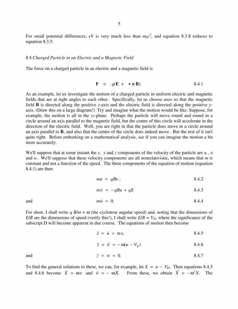
Examples of these trajectories are shown in figure VIII.4, though I’m afraid you will have to turn your monitor on its side to view it properly. They are drawn for s = 0.25, 0.50, 1.00 and 2.00, where s is the ratio of the constant electron speed to the characteristic speed SC. The wire is supposed to be situated along the z-axis (ρ = 0) with the current flowing in the direction of positive z. The electron drifts in the opposite direction to the current. (A positively charged particle would drift in the same direction as the current.) Distances in the figure are expressed in terms of the perineme distance ρ0. The shape of the path depends only on s (and not on ρ). For no speed does the path have a cusp. The radius of curvature R at any point is given by R = ρ/s. Minima of ρ occur at ρ = ρ0 and θ = (4n + 1)π/2 , where n is an integer; Maxima of z occur at s

e0ρ=ρ and θ = (4n + 2)π/2 ; Maxima of ρ occur at s

e2

0ρ=ρ and θ = (4n + 3)π/2 ; Minima of z occur at s

e0ρ=ρ and θ = (4n + 4)π/2 . The distance between successive loops and the period of each loop vary rapidly with electron speed, as is illustrated in Table VIII.2. In this table, s is the electron speed in units of the characteristic speed SC, A1 is the ratio of aponeme to perineme distance, A2 is the ratio of interloop distance to perineme distance, A3 is the ratio of period per loop to ρ0/SC, and A4 is the drift speed in units of the characteristic speed SC .

14

FIGURE VIII.4

For example, for a current of 1 A, the characteristic speed is 3.5176 × 104 m s−1. If an electron is accelerated through 8.7940 V, it will gain a speed of 1.7588 m s−1, which is 50 times the characteristic speed. If the electron starts off at this speed moving in the same direction as the current and 1 Å (10−10 m) from it, it will reach a maximum distance of 8.72 × 1010 megaparsecs ( 1 Mpc = 3.09 × 1022 m) from it, provided the Universe is euclidean. The distance between the loops will be 1.53 × 1012 Mpc, and the period will be 8.60 × 1020 years, after which the electron will have covered, at constant speed, a total distance of 1.55 × 1012 Mpc. The drift speed will be 1.741 × 106

m s−1.

15

TABLE VIII.2

s A1 A2 A3 A4

0.1 1.22 3.47 × 10−2 6.96 4.99 × 10−3

0.2 1.49 1.54 × 10−1 7.75 1.99 × 10−2

0.5 2.72 1.34 11.0 0.122

1.0 7.39 9.65 21.6 0.447

2.0 54.6 1.48 × 102 1.06 × 102 1.40

5.0 2.20 × 104 1.13 × 105 2.54 × 104 4.49

10.0 4.85 × 108 3.70 × 109 3.90 × 108 9.49

20.0 2.35 × 1017 2.59 × 1018 1.33 × 1017 19.5

50.0 2.69 × 1043 4.73 × 1044 9.55 × 1042 49.5

Let us now turn to consideration of cases where ,00 ≠v so that the motion of the electron is not restricted to a plane. At first glance is might be thought that since an azimuthal velocity component gives rise to no additional Lorenz force on the electron, the motion will hardly be affected by a nonzero v0, other than perhaps by a revolution around the wire. In particular, for given initial velocity components u0 and w0, the perineme and aponeme distances x1 and x2 might seem to be independent of v0 . Reference to Table VIII.1, however, shows that this is by no means so. The reason is that as the electron moves closer to or further from the wire, the changes in v made necessary by conservation of the z-component of the angular momentum are compensated for by corresponding changes in u and w made necessary by conservation of kinetic energy. Since the motion is bounded above and below, there will always be some time when .0=ρ& There is no loss of generality if we shift the time origin so as to choose 0=ρ& when t = 0 and x = 1. From this point, therefore, we shall consider only those trajectories for which u0 = 0. In other words we shall follow the motion from a time t = 0 when the electron is at an apsis ( 0=ρ& ). [The plural of apsis is apsides. The word apse (plural apses) is often used in this connection, but it seems useful to maintain a distinction between the architectural term apse and the mathematical term apsis.] Whether this apsis is perineme (so that 10101 ,, ww ==ρ=ρ vv& ) or aponeme (so that

20202 ,, ww ==ρ=ρ vv& ) depends on the subsequent motion. The electron starts, then, at a distance from the wire defined by x = 1. It is of interest to find the value of x at the next apsis, in terms of the initial velocity components v0 and w0. This is found

16

from equation 8.5.10 with u = 0 and u0 = 0. The results are shown in figure VIII.4. This figure shows loci of constant next apsis distance, for values of x (going from bottom left to top right of the figure) of 0.05, 0.10, 0.20, 0.50, 1, 2, 5, 10, 20, 50, 100. The heavy curve is for x = 1. It will immediately be seen that, if ,2

00 v−>w (above the heavy curve) the value of x at the second apsis

is greater than 1. (Recall that v and w are dimensionless ratios, so there is no problem of dimensional imbalance in the inequality.) The electron was therefore initially at perineme and subsequently moves away from the wire. If on the other hand ,2

00 v−<w (below the heavy curve) the value of x at the second apsis is less than 1. The electron was therefore initially at aponeme and subsequently moves closer to the wire.

0 0.5 1 1.5 2-2

-1.5

-1

-0.5

0

0.5

1

1.5

2

|v0|

w0

FIGURE VIII.4

The case where 200 v−=w is of special interest, for then perineme and aponeme distances are equal

and indeed the electron stays at a constant distance from the wire at all times. It moves in a helical trajectory drifting in the opposite direction to the direction of the conventional current I. (A positively charged particle would drift in the same direction as I.) The pitch angle α of the helix (i.e. the angle between the instantaneous velocity and a plane normal to the wire) is given by

,/tan vw−=α 8.5.19

where w and v are constrained by the equations

5

17

200 v−=w 8.5.20

and .222 sw =+v 8.5.21

This implies that the pitch angle is determined solely by s, the ratio of the speed S of the electron to the characteristic speed SC. On other words, the pitch angle is determined by the ratio of the electron speed S to the current I. The variation of pitch angle α with speed s is shown in figure VIII.6. This relation is entirely independent of the radius of the helix.

0 2 4 6 8 10 12 14 16 18 200

10

20

30

40

50

60

70

80

90

Pitch a

ngle

α

Speed s

FIGURE VIII.5

If ,200 v−≠w the electron no longer moves in a simple helix, and the motion must be calculated

numerically for each case. It is convenient to start the calculation at perineme with initial

conditions .1,,0 02000 =−>= xwu v For other initial conditions, the perineme (and aponeme)

values of u, v, w and ρ can easily be found from equations 8.5.10 (with u0 = 0), 8.5.8 and 8.5.9. Starting, then, from perineme, integrations of these equations take the respective forms

∫−−+−

ρ=

x

dxxxwxS

t1

2/120

220

C

0 ,])(lnln2)/11([v 8.5.22

6

18

∫−−+−ρ−=

x

dxxxxwxtSwz1

2/120

2200C0 ln])(lnln2)/11([v 8.5.23

and ∫−−−+−=φ

x

dxxxxwx1

22/120

2200 .])(lnln2)/11([vv 8.5.24

The integration of these equations is not quite trivial and is discussed in the Appendix (Section 8A).

In general the motion of the electron can be described qualitatively roughly as follows. The motion is bounded between two cylinders of radii equal to the perineme and aponeme distances, and the speed is constant. The electron moves around the wire in either a clockwise or a counterclockwise direction, but, once started, the sense of this motion does not change. The angular speed around the wire is greatest at perineme and least at aponeme, being inversely proportional to the square of the distance from the wire. Superimposed on the motion around the wire is a general drift in the opposite direction to that of the conventional current. However, for a brief moment near perineme the electron is temporarily moving in the same direction as the current.

An example of the motion is given in figures VIII.7 and 8 for initial velocity components u0 = 0, v0 = w0 = 1. The aponeme distance is 11.15 times the perineme distance. The time interval between two perineme passages is 26.47 ρ0/SC . The time interval for a complete revolution around the wire (φ = 360o) is 68.05 ρ0/SC . In figure VIII.8, the conventional electric current is supposed to be flowing into the plane of the “paper” (computer screen), away from the reader. The portions of the electron trajectory where the electron is moving towards from the reader are drawn as a continuous line, and the brief portions near perineme where the electron is moving away from the reader are indicated by a dotted line. Time marks on the figure are at intervals of 5ρ0/SC .

19

FIGURE VIII.7

FIGURE VIII.8

20

8A Appendix. Integration of the Equations

Numerical integration of equations 8.5.22-24 is straightforward (by Simpson’s rule, for example) except near perineme (x = 1) and aponeme (x = x2), where the integrands become infinite. Near perineme, however, we can substitute

ξ+= 1x and near aponeme we can substitute ),ξ−= 1(2xx and we can expand the integrands as power series in

ξ and integrate term by term. I gather here the following results for the intervals x = 1 to x = 1 + ε and x = x2 − ε to x = x2, where ε must be chosen to be sufficiently small that ε4 is smaller than the precision required.

)1(])(lnln2)/11([ 317

121

1

1 51

1312/12

022

01 K+ε+ε+ε+=−+−= ∫ε+

−CBAMdxxxwxI v 8A.1

)(ln])(lnln2)/11([ 317

121

1

1 51

312/12

022

02 K+ε+ε+ε=−+−= ∫ε+

−EDMxdxxxwxI v 8A.2

)1(])(lnln2)/11([ 317

121

1

1 51

13122/12

022

03 K+ε+ε+ε+=−+−= ∫ε+

−−HGFMdxxxxwxI v 8A.3

))/()/(/1[])(lnln2)/11([ 3227

12225

1223

12/120

2204

2

2

K+ε+ε+ε+=−+−= ∫ ε−

− xCxBxANdxxxwxIx

xv

8A.4

∫ ε−

−−+−=2

2

ln])(lnln2)/11([ 2/120

2205

x

xxdxxxwxI v

])/()/(/[ln 3227

12225

123

124 K+ε+ε+ε−= xExDxNxI 8A.5

∫ ε−

−−−+−=2

2

22/120

2206 ])(lnln2)/11([

x

xdxxxxwxI v

22

3227

12225

1223

1 /])/()/(/1[ xxHxGxFN K+ε+ε+ε+= 8A.6

The constants are defined as follows.

2/1

020

2

+

ε=

wM

v 8A.7

2/1

02

202

2

)/(ln2

−−

ε=

wxx

xN

v 8A.8

)(213

020

020

1w

wa

+

++−=

v

v 8A.9

)(2

14

020

0322

01

w

wb

+

++=

v

v 8A.10

21

)(2

5

020

1211

0212

01

w

wc

+

++−=

v

v 8A.11

( )202

20

202

202 ln)/(2

1ln)/(3xwx

xwxa

−+

+−+=

v

v 8A.12

( )202

20

20322

202 ln)/(2

1ln)/(4

xwx

xwxb

−+

+−+=

v

v 8A.13

( )202

20

1211

221

0212

202 ln)/(2

ln)/(5

xwx

xwxc

−+

+−+=

v

v 8A.14

nn aA 21−= 8A.15

283

21

nnn abB +−= 8A.16

3165

43

21

nnnnn abacC −+−= 8A.17

n

nn AD )1(21 −+= 8A.18

31

21 )1( +−+= n

n

nn ABE 8A.19

n

nn AF )1(2 −+= 8A.20

3)1(2 +−+= n

n

nn ABG 8A.21

n

nn

n

nn ABCH )1(43)1(2 −++−+= 8A.22

2,1=n