on the differential equations of the electrodynamics for ... fileon the differential equations of...

C:\German\Wien_5d.doc 01-11-12

W. Wien — Annalen der Physik [4te Folge], 13(4) — 8 März, 1904 Translation & type-setting © R.R.Traill (2008) 5d

On the differential equations of the electrodynamics for moving bodies;

by W.Wien — 1904

From the two-part German narrative (here also republished as parallel text): Über die Differentialgleichungen der Elektrodynamik für bewegte Körper

Translated, typeset, and edited

by Robert R. Traill

published online by: Ondwelle Publications, 29 Arkaringa Cres., Black Rock 3193, Vic., Australia and by the General Science Journal — www.wbabin.net

10 August 2008

Translation and typesetting : © Copyright R.R.Traill, 2008. Users are permitted to use this translation for single-copy non-commercial purposes provided that the original authorship is properly and fully attributed to both author and publisher. If an article is subsequently reproduced or disseminate not in its entirety but only in part or as a derivative work, this must be clearly indicated. For commercial or multi-copy permissions, please contact Copyright Agency Limited: [email protected]

ÜBERSETZERS EINLEITUNG

Von 1851 bis 1905, es gab eine Reihen interessante „Vorrel-atiität“ Entwicklungen in der Theorie der Lichtfortpflanzung. Diese Verhandlungen wurde durch Einsteins 1905 Schrift gekürzt — und dann im Chaos von zwei Weltkriegen vergessen. Das Einstein-Minkowski Bericht selbst als Technologie sehr groß erfolgreich gewesen ist;— aber setzt Besorgnis fort daß diese Formulierung fehlerhaftig als reine Wissenschaft ist und bleibt. So kann es etwas Wert geben, wenn man die früheren Arbeiten wieder studiert, — teils um von ihren mathematischen Techniken zu profitieren — und besonders wann immer jede mögliche Art „des Äthers“ oder „des kumulativen Resident-feldes“ berücksichtigt ist.

Hier stelle ich ein zweiteiliges Bericht von W.Wien dar, aber ich gebe gleichzeitig eine ähnliche Übersetzung des E.Cohn Bericht heraus (zusammen mit seinem späteren Antwort auf Wiens Kritik). — Sehe die „Consolidated References“ an der letzten Seite beider Übersetzungen. (Die gleiche Liste für beide, aber anders sortiert). Andere hervorgehobene Namen auch merken, die Aufmerksamkeit verdienen.

Das Ende jeder Originalseite (z.B. S.650), wird durch „<650>“ bedeutet; (u.s.w.). Zusätze zum ursprünglichen Bericht werden durch (i) Fußnoten mit Buchstaben, z.B. F markiert; und/oder (ii) eckige Klammern: […] und/oder (iii) offensichtliche neuere Anachronismen. Es gibt ein kurtzer Inhalt am Seite 22.

RRT, Melbourne, 10. August 2008

TRANSLATOR’S PREFACE

From 1851 to 1905, there were a series of interesting “pre-relativity” developments in the theory of light transmission. This approach was cut short by Einstein’s 1905 paper, and then forgotten in the chaos of two world wars. The Einstein-Minkow-ski account itself has been hugely successful as technology ;— but there is continuing disquiet that somehow this formulation doesn’t make sense as pure science. Thus there may be some value in re-examining the earlier works, — partly to benefit from their mathematical techniques — and especially whenever any sort of “aether” or “resident cumulative field” is under consider-ation.

Here I present a two-part account by W.Wien, but I am simultaneously issuing a similar translation of E.Cohn’s account (together with his later reply to Wien’s criticism). — See the “Consolidated References” on the last page of both translations. (The same list for both, but sorted differently). Also note other highlighted names which deserve attention.

The end of each original page (e.g. p.650), is indicated by “<650>” etc. Additions to the original account are marked by (i) foot-notes using capital letters, e.g. F ; and/or (ii) square brackets : […], and/or (iii) obvious later anachronisms. There is a brief “Contents” table on page 22.

RRT, Melbourne, 10. August 2008

The 2008 version used “ParkAvenue BT” font as more readable than Wien’s

“Fraktur/Old English” font: E, H, S...(=E, H, S,…) for special cases. Although the replacement symbols appeared on the screen, it seems that they usually vanished during printing! Hence I have now restored Wien’s original font.

With apologies; RRT, 30-10-2012.

Die Version 2008 verwendet „ParkAvenue BT“ Schriftart als besser lesbar als Wiens „Fraktur / Old English“ Schriftart: E, H, S, ...(=E,H,S,...) für besondere Fälle. Obwohl die Ersatz-Symbolen auf dem Bildschirm erschien, scheint es, dass sie in der Regel verschwand während des Druckens! Daher habe ich jetzt die ursprüngliche Schriftart wiederhergestellt. — Mit Entschuldigungen; RRT, 30-10-2012

W.Wien (1904) differential equations 2 of 23 of electrodynamics for moving bodies


Über die Differentialgleichungen der Elektrodynamik für bewegte Körper;

von W.Wien I

Von den bisher Aufgestellten Differentialgleichungen, welche die Maxwellsche Theorie für den Fall der Bewegung verallgemein-ern, hat sich die von H.A.Lorentz1 am besten bewährt. Die Theorie von H.Hertz2, wonach der Träger der elektromagnet-ischen Wirkungen sich mit derselben Geschwindigkeit bewegen soll, wie die Materie, wird durch den von Michelson und Morley3 wiederholten FizeauschenA Versuch widerlegt, der zeigt, daß ein Lichtstrahl von bewegtem Wasser nur in mit einem bestimmten Bruchteil der Geschwindigkeit mitgezogen wird. Da bisher alle Versuche eine Bewegung des Lichtäthers in dem von Materie freien Raum nachzuweisen gescheitert sind, liegt für die Theorie keine Veranlassung vor, sich mit der Komplikation einer derartigen Möglichkeit zu befassen.

Neuerdings ist von E.Cohn4 ein System von Gleichungen für bewegte Körper aufgestellt, das in der Tat zunächst geeignet erscheint, den beobachteten Tatsachen gerecht zu werden. So hat er vor dem Lorentzschen sogar den Vorzug, das negative Ergebnis des Michelsonschen Interferenzversuches ohne Zuhilfe-nahme einer weiteren Hypothese zu erklären, während Lorentz die Annahme machen muß, daß die Dimensionen der festen Körper von der Geschwindigkeit abhängig sind.

Dagegen enthält die Theorie von Cohn wieder in anderer Hinsicht Schwierigkeiten. <641>

Bezeichnen wir den elektrischen Vektor mit E, den magnet-ischen mit H, die Lichtgeschwindigkeit mit c, die Translations-geschwindigkeit mit v, so lauten die Differentialgleichungen von Cohn in bekannten Vektorsymbolen für den freien Äther, bezogen auf relative Koordinaten

.

Bei stationärer Bewegung eines geladenen Körpers würden daher die Differentialgleichungen direkt in die eines ruhenden Körpers übergehen und nur eine magnetische Wirkung, dem Biot-Savartschen Gesetz entsprechend, übrig bleiben. Diese Folgerung steht mit der Heavisideschen Lösung der Feld-gleichungen bewegter Ladungen im Widerspruch und da diese

1 H.A.Lorentz, Versuch einer Theorie der elektrischen und optischen Erscheinungen in bewegten Körpern. Leiden 1895. [Also in his Collected Papers,

vol. 5, pp.1-138. Martinus Nijhoff: The Hague. (1935)].

2 H.Hertz, Wied. Ann. 41. p.369. 1890. [= Annalen der Physik (series 2); “Ueber die Grundgleichungen der Elektrodynamik für bewegte Körper”] 3 W.A.Michelson u. E.W.Morley, Amer. Journ. of Science (3) 31. p.377. 1886. [“Influence of Motion of the Medium on the Velocity of Light”; 377-

386] A Fizeau (1859 Sep). Ann. Chim. Phys. (3), 57, 385-. — more recently discussed by (e.g.) I.Lerche (1977 Dec), “The Fizeau Effect: Theory, experiment,

and Zeeman’s measurements”. Amer. J. Phys., 45(12), 1154-1163. 4 E.Cohn, Ann d. Phys. 7. p29. 1902. [Series 4; “Ueber die Gleichungen des elektromagnetischen Feldes für bewegte Körper”; 29-56; — follow link

from www.weltderphysik.de/de/3001.php?bd=318 for a facsimile of the original. An English+German text is at www.ondwelle.com/cohn ].

On the differential equations of the electrodynamics for moving bodies;

by W.Wien I

Of the hitherto established differential-equations which generalize the Maxwellian theory for the case of motion, those of H.A.Lorentz1 are best verified. The theory of H.Hertz2, for which the carrier of the electro-magnetic effects should move with the same speed as the matter, is refuted by the FizeauA investigation, repeated by Michelson and Morley3. This shows, that a light-ray will be dragged along by moving water only up to a certain fraction its velocity. As hitherto all investigations have failed to prove any motion of light-aether in matter-free space, no suggestion has been offered to deal with the complication of such a possibility.

Recently E.Cohn4 established a system of equations for moving bodies, which actually appears closest to being suitable to accord with the observed facts. Thus he had the advantage, even over Lorentz, of explaining the negative result of Michelson’s interference experiment without the help of a further Hypothesis — while Lorentz must make the assumption that the dimensions of solid bodies are dependent on the velocity.

Against that, Cohn’s theory contains further difficulties in another respect. <641>

We designate the electrical vector with E, the magnetic with H, the light-speed with c, the speed of matter-translation with v. Thus we can state Cohn’s differential equations in well-known vector-symbols for the free aether, expressed with respect to relative coordinates

For unaccelerated motion of a charged body, the differential-equations would thus turn directly into those of a resting body, and the only remaining magnetic effect would be that corresponding to the Biot-Savart law. This conclusion contradicts Heaviside’s solution of the field-equat-ions for moving charges; and since this latter has received compre-

∂D ∂B ∂t ∂t D = E – H , B = E + H .

= c rot H , = – c rot E ,

v v c c [ ] [ ]

0a Note: rot ... ≡ curl ... ≡ ∇∇∇∇× ...

RRT (2008)

and in modern notation, […] would be: “ (v/c) × H” i.e., a vestor “cross product” RRT (2012)



durch die Versuche von KaufmannB eine weitgehende Bestätigung erfahren hat, so scheint mir die Theorie von Cohn nicht mit den Tatsachen in Übereinstimmung zu stehen, wenn nicht eine Verschiedenheit der elektromagnetischen Energie, je nachdem die Erregung von bewegten oder von ruhenden Körpern ausgeht, angenommen wird. Dies würde wieder zu neue prinzipiellen Schwierigkeiten führen.

Eine andere Schwierigkeit erwächst der Cohnschen Theorie aus der Fortpflanzungsgeschwindigkeit eines von einer bewegten Quelle ausgehenden Lichtstrahles.

Nehmen wir als Richtung des Strahles die x-Achse und den, in derselben Richtung sich bewegenden, leuchtenden Punkt unendlich entfernt, so daß wir nur ebene Wellen zu betrachten haben. Die y-Achse soll dem elektrischen Vektor parallel sein. Dann sind nur Ey und Hz von Null verschieden und wir haben die Gleichungen

.

Durch Elimination von Hz ergibt sich

.

oder wenn wir 1–v2/c2 = κκκκ2 setzenC

.

<642>

Setzen wir einer ebenen Welle entsprechend

so wird

.

woraus die Fortpflanzungsgeschwindigkeit

.

folgt.

Dies ist die auf relative Koordinaten bezogene Geschwindigkeit.

Bringt man den betrachteten Punkt durch Hinzufügen einer Geschwindigkeit –v in absolute Ruhe, so ist die absolute Geschwindigkeit des Strahles

.

Es würde sich daher ein Lichtstrahl, der von einem bewegten leuchtenden Punkt kommt, schneller fortpflanzen als wenn er von einem ruhenden ausgegangen wäre und zwar in ersten Näherung unabhängig von der Bewegungsrichtung des leuchtenden Punktes, ein Resultat, das die Konstanz der Lichtgeschwindigkeit und damit die Grundlagen der Maxwellschen Theorie angreifen würde.

B Presumably: W.Kaufmann, Physikalische Zeitung, 4, p.54-57 (1902) “Die elektromagnetische Masse des Elektrons” [as a function of velocity] &/or Gött.Nachrichtungen Math. phys. Kl., (1903). — Results of both were cited and used in: H.A.Lorentz (1904) Proc.Acad.Sciences Amsterdam, 6. A subsequent Kaufmann paper of potential interest is: Annalen der Physik (series 4), 19, 487, (1906).

C Wien here follows Heaviside (1900 June 8: The Electrician, 45, p245) in using kappa (κκκκ), though Wien’s original text actually uses a different font (κ) which is unhelpfully similar to “x”. In contrast, Lorentz (1904: Proc.Acad.Sci.Amsterdam, 6) uses “1/β”. Einstein (1905 Sep) later does likewise.

hensive confirmation through the investigations by KaufmannB, it thus seems to me that Cohn’s theory is not in accord with the facts, — given that not one difference of the electromagnetic energy will be accepted to distinguish between the emissions of moving or resting bodies. This would again lead to new principal difficulties.

Another difficulty arises in Cohn’s theory from the speed-of-propagation of an emitted light ray from a moving source .

Let us take the x-axis as the direction of the ray, and the same direction for the light-emitting point, which we also take as infinite-ly far away, so that we only have to consider plane wavefronts. Thus the y-axis will be parallel to the electrical vector. Then only Ey and Hz are different from zero and we have the equations

Through the elimination of Hz we get

or if we setC 1–v2/c2 = κκκκ2 then

<642>

If we set up a plane wave corresponding to

then from which follows the propagation-speed:

This is the velocity based on relative coordinates.

If one imposes on the point a speed of –v in absolute-rest-coordinates, then the ray’s absolute velocity is

This would therefore be a light ray coming from a moving luminous point, and hence travelling faster than if it were emitted from a resting source. Of course, as a first approximation, it would be independent of the luminous point’s direction-of-motion —

∂Ey v ∂Hz ∂Hz ∂t c ∂t ∂t ∂Hz v ∂Ey ∂Ey ∂t c ∂t ∂t

– = – c ,

– = – c .

∂2Ey ∂2

Ey ∂2Ey

∂t2 ∂x∂t ∂x2

κκκκ2 + 2 v = c2 ,

Ey = A e i ( n t – b z) ,

κκκκ2 n2 – 2 n b v = c2 b2

n v + √(v2 + c2 κκκκ2) c + v

b κκκκ2 κκκκ2

= =

c + v v2 v3 κκκκ2 c2 c3

– v = c 1 + + + . . . . ( )

∂2Ey ∂2

Ey v2 ∂2Ey ∂2

Ey ∂t2 ∂x∂t c2 ∂t2 ∂x2

+ 2 v – = c2 ,

0b

0c

0d

0e

0f

0g

0h



Denn es muß für die Fortpflanzungsgeschwindigkeit einer einmal von der Strahlungsquelle losgelösten Strahlung gleichgültig sein, ob sich diese bewegt hat oder nicht.

Der größte Teil der Schwierigkeiten für die Theorie der Elektrodynamik bewegter Körper rührt davon her, daß man einerseits die Bewegungsmöglichkeit des Äthers in die Theorie aufnehmen wollte, anderseits eine Trennung von Äther und Materie für nötig hielt. Stellt man sich dagegen auf den zuerst von Lorentz eingenommen Standpunkt, daß alle Wechselwirkung zwischen Äther und Materie nur durch die Elementarladungen der Atome hervorgerufen werden, so fallen fast alle jene Schwierigkeiten von selbst fort und das Maxwellsche System für ruhende Körper genügt völlig, um auch die Elektrodynamik bewegte Körper ohne Zuhilfenahme irgend einer Hypothese zu umspannen. Da von anderen Seite die<643> chemischen Eigenschaften der Körper notwendig fordern, die Kontinuität der Materie aufzugeben und die Materie als aus Elementarquanten in unstetiger Weise bestehend anzunehmen, so scheint mir um so mehr die Annahme dieses Systems geboten.

Hiernach ist ein Bewegungsvorgang für die Elektrodynamik die Bewegung einer Elementarladung durch den Raum. Es ist dies ein Vorgang, der noch vollständig in die Theorie ruhender Körper gehört. Denn daß sich ein Quantum Elektrizität bewege, und welche elektromagnetischen Wirkungen dadurch hervorgerufen werden, das vermag die Maxwellsche Theorie ohne weiteres zu behandeln. Solange es sich um geordnete Bewegung handelt, d.h. die Kom-plikationen der Wärmelehre nicht mitspielen, ist es im allgemeinen vollständig ausreichend, die Bewegung einer einzigen Elementar-ladung zu verfolgen. Jedenfalls gehören die Erscheinungen, die auf der Wechselwirkung vieler Atome beruhen, zu denen, die eine genauere Behandlung vorläufig ausschließen.

Aus diesem Grunde ist auch das allgemeine Integral, das Lorentz5 als Lösung seiner Gleichungen für die Wirkung der Bewegung beliebig vieler Atome benutzt, zwar für prinzipielle Untersuchungen von großem Werte, für die Behandlung des Problems der Bewegung eines einzelnen Elementarquantums, eines „Elektrons“ weniger geeignet, weil es für diesen Spezial-fall zu kompliziert ist. Infolgedessen ist auch die Theorie bewegter Elektronen über den bereits von HeavisideD erledigten Fall, der Bewegung mit konstanter Geschwindigkeit, nicht erheblich hinausgekommen.

5 H.A.Lorentz, Théorie électrique de Maxwell et son application aux corps mouvants p.119. Leiden 1892.

Der erste Beweis dieses Satzes ist von Lorenz gegeben [=The first demonstration of this proposition is given by L.Lorenz]: Pogg. Ann. 131. p.243-263. 1867. [=Annalen der Physik (series 1)]

D Oliver Heaviside •(1900-1902): “Electromagnetic Theory — CXII-CXXVI” The Electrician, 44 (#18: 23 Feb 1900), 615- , continuing in episodes to 48 (Jan 1902?), -221; republished (with added subheadings) as Chapter 9 “Waves from moving sources” in his Electromagnetic Theory , vol. III (1912). •(1902 Feb 14 - June 6). Sequel :“... CXXVII-CXXVIII” ibid; then continued in Nature (Oct 30 (p6), Nov 6 (p32); 1903 Jan 1 (p202), 1904 Jan 28 (p293), 1904 Feb 11 (p342), 1903 Jan 29 (p297)... republished in that order, as Chapter 10 “Waves in the Ether” in his EMT III (1912). RRT.

a result that would clash with the constancy of light-speed and hence with the foundations of the Maxwellian theory.

In that case each ray emitted from the source must have the same propagation-velocity, nomatter whether or not that source is in motion.

The greatest part of the difficulties for the theory of the electrodynamics of moving bodies comes from this: that on the one hand one wants to assume within the theory that the aether can move, but on the other hand one expects a necessary separation between aether and matter. If against that, one adopts the standpoint first taken by Lorentz, that all interaction between aether and matter occurs only through the elementary charges of the atoms, then nearly all the difficulties fall away automatically — and the Maxwellian system for station-ary bodies suffices fully to also include the electrodynamics of moving bodies, without the assistance of any further hypothesis. Then on the other hand, the<643> chemical properties of the body necessarily require one to give up the continuity of matter and to assume that matter exists in transformable elementary quanta; so the assumption of this system seems to me to be so much the more imperative.

Next there is a motion-scenario for the electrodynamics of the progress of an elementary charge through space. It is this single scenario which still completely falls within the theory of stationary bodies. Unless a quantum of electricity moves, and thereby stimulates some electromagnetic activity, the Maxwellian theory is unable to process anything. As long as it is concerned with orderly motion, i.e. the complic-ations of heat-theory do not play a part, it is generally quite feasible to trace a single elementary charge. In any case, phenomena which are based on the interaction of many atoms, are cases for which exact treatment is provisionally excluded.

For this reason Lorentz’s5 general integral is poorly suited because it is too complicated for this special case. (This integral is the solution to the random motion-activity of many atoms — indeed a major investigation of great value for the treatment of the motion of a simple elementary quantum of an “electron”.) Consequently the theory of moving electrons is not assisted appreciably — except for the special case already developed by Heaviside,D of motion with constant velocity.



Von Wichtigkeit ist die zuerst ebenfalls von Lorentz eingeführte, dann von Abraham6 auf Grund der Poincaréschen7 „elektromagnetischen Bewegungsgröße“ abgeleiteten Unterscheidung zwischen „longitudinaler“ und „transversaler“ Masse, deren quantitative Messung indessen auf Anwendung der Maxwellschen ponderomotorischen Wirkungen und demnach auf einer sehr wahrscheinlichen, aber nicht ganz hypothesenfreien Grundlage beruht. <644>

Es soll im folgenden zunächst gezeigt werden, daß man zu einem mit dem Lorentzschen System der Elektrodynamik überein-stimmenden gelangt entweder wenn man ein Elektron als ruhend annimmt und den Äther mit der entgegengesetzten Geschwindig-keit strömen läßt, wobei dann der Einfluß der Bewegung nach Analogie der EulerschenE hydrodynamischen Geschwindigkeit in der Weise einzuführen ist, daß man [→] setzt, oder indem man die gewöhnlichen Maxwellschen Gleichungen be-nutzt und die Ladung mit ihrer Geschwindigkeit sich bewegen läßt. Wir werden damit gleichzeitig ein Integral erhalten, das die Verallgemeinerung eines für die Ruhe bekannten elektromagnet-ischen Vorganges für eine beliebige Bewegung mit konstanter Geschwindigkeit enthält.

1. Beziehung der Lorentzschen Gleichungen zu denen für ruhende Körper.

Wir legen die x-Achse in die augenblickliche Bewegungsricht-ung und nehmen im übrigen an, daß die Geschwindigkeit eine beliebige kontinuierliche und differenzierbare Funktion der Zeit ist, und setzen - - - -

dann erhalten wir das Gleichungssystem für diese Bewegung, wenn wir in das für ruhende Körper anstatt d/dt jetzt ∂/∂t – v ∂/∂x setzen

(1)

Elimination von E und H gibt die allgemeine Gleichung

(2) <645>

Wir führen nun zwei neue Variabele ξ und η anstatt t und x ein mit Hilfe der Gleichungen (3)

Anstatt der Gleichung (2) erhalten wir dann die neue

6 M.Abraham, Ann. d. Phys. 10. p.105. 1903. [(series 4); “Prinzipien der Dynamik des Elektrons”, pp.105-179.

Follow link from www.weltderphysik.de/de/3001.php?bd315 for a facsimile of the original. RRT]

7 H.Poincaré, Festschrift für H.A.Lorentz, p.252. Leiden 1900. E [Euler, L., (1766/1808). “Reserches sur l’intégration de l’équation (ddz/dt2) = aa(ddz/dx2) + b/x •(dz/dx) + (c/xx).z ” — Opera Omnia (ser.1), 23, 42-73.]

Of importance is the distinction between “longitudinal” and “transverse” mass, also first introduced by Lorentz and then derived by Abraham6 from the “electromagnetic” motion-magnitude” of Poincaré.7 Meanwhile the quantitative measurement of this distinction is based on the use of the Maxwellian ponderomotor effect, and accordingly on an apparently hypothesis-free basis — though that is not as true as it seems. <644>

In the following account it will be shown that electrodynamics does agree with the Lorentz system, either (i) if we assume the electron is at rest, and that the aether is allowed to flow in the opposite direction, whereby the influence of motion is introduced as an analogy to the EulerianE hydrodynamic velocity, so that one sets: or (ii) if we use the usual Maxwell equations and let the charge move with its own velocity. We will thereby simultaneously obtain an integral, which formulates the generalization (from the known rest-state), of any electromagnetic event now travelling at any given constant velocity.

1. Relationship between the Lorentz equations and those for resting bodies.

We let the x-axis lie in the instantaneous direction of motion, and for remaining instants we assume that the velocity is an arbitrary continuous-and-differentiable function of time, and set ←

then we get the equation-system for motion if, instead of d/dt we now use ∂/∂t – v ∂/∂x to set

Elimination of E and H gives us the generalized equation

<645>

We now introduce two new variables ξ and η instead of t and x, with help from the equations ←

Instead of equation (2) we get the new one:

∂E ∂E ∂ t ∂ x ∂H ∂H ∂ t ∂ x

– vx = c rot H ,

– vx = – c rot E ,

Again: rot ... ≡ curl ... ≡ ∇∇∇∇× ...

RRT (2008)

∂2 φ ∂2 φ ∂2 φ df ∂ φ ∂2 φ ∂2 φ ∂t2 ∂x∂t ∂x2 dt ∂ x ∂ y2 ∂ z2

– 2f + (f2 – c2) – = c2 + . .

( )

ξ = α t + β φ(t) + γ x φ(t) = ∫ f(t) dt .

η = α1 t + β1 φ(t) + γ1 x

∂ ∂ t RRT

ie = – v • ∇∇∇∇ d ∂ ∂ ∂ ∂ d t ∂ t ∂ x ∂ y ∂ z

= – vx – vx – vx

vx = f(t) = v ,

0i

0j



(4)

Wir können diese Differentialgleichung auf die zurückführen, die aus (2) entsteht, wenn vx = 0 gesetzt wird. Zu dem Zweck verlangen wir, daß die Faktoren von

verschwinden sollen.

Nun ist

(5)

wenn die Faktoren von ∂φ/∂ξ und ∂φ/∂η verschwinden sollen. Der Faktor von ∂2φ/∂ξ∂η verschwindet, wenn außerdem noch α α1 = c2γ γ1 ist. Wir behalten dann die Gleichung

die von derselben Form, wie die gewöhnlicheF

<646>

ist, wenn wir in dieser anstatt x die Größe η c/√(α1

2 –c2γ12)

anstatt c die Größe c/√(α2 –c2γ2) setzen. Das Integral F(ct – r)/r, r2 = x2 + y2 + z2 der gewöhnlichen Gleichung geht daher für unsere in das

über.

Bestimmt nun der Punkt r = 0 die Lage des Elektrons, so darf, da wir von der Vorstellung ausgegangen sind, daß das Elektron ruht und der Äther sich an ihm vorbeibewegt, r die Zeit nicht enthalten, d.h. η muß von der Zeit unabhängig sein. Wenn wir das erreichen wollen, müssen wir in (3) γ1 = ∞ setzen. Aus (5) folgt aber β1 = γ1 = ∞, so daß wir die gewünschte Unabhängigkeit überhaupt nicht erreichen können. Vielmehr ist für γ1 = ∞

F Here Wien’s original text uses “ ∆” instead of “∇2” for this standard wave-equation! — Much earlier, L.Lorenz (1867: Pogg.Ann., 131, p251)

had used “ ∆2” for this purpose, so Wien’s “ ∆” is probably a corrupted version of that notation. — RRT (2008)

We can refer this differential equation back to the one which arose out of (2) when vx = 0 . For this purpose, we need the factors

←

to vanish.

Now we have ←

if the factors ∂φ/∂ξ and ∂φ/∂η are to vanish. Additionally the factor ∂2φ/∂ξ∂η disappears whenever α α1 = c2γ γ1 . We then get the equation

which is in the usual [wave-equation] formF

← <646>

if we here put: the value η c/√(α1

2 –c2γ12) instead of x — and

the value c/√(α2 –c2γ2) instead of c. The integral F(ct – r)/r, r2 = x2 + y2 + z2 of the usual equation, transforms for ours into:

Now set the point r = 0 as the position of the electron. Since we envisage that the electron is at rest, and that the aether is moving past it, [the formula for] r cannot contain time; i.e. η must be independent of time. If we want to achieve that, we must set γ1 = ∞ in (3). However it follows from (5) that β1 = γ1 = ∞, so that the desired independence is absolutely unobtainable. Indeed, for γ1 = ∞

∂2 φ ∂ ξ ∂ ξ ∂ ξ ∂ ξ ∂ ξ ∂ t ∂ t ∂ x ∂ x ∂2 φ ∂ η ∂ η ∂ η ∂η ∂ η2 ∂ t ∂ t ∂ x ∂x ∂2 φ ∂ ξ ∂ η ∂ ξ ∂ η ∂ η ∂ξ ∂ ξ ∂ η ∂ξ ∂η ∂ t ∂ t ∂ t ∂ x ∂ t ∂x ∂ x ∂ x ∂ φ ∂2 ξ df ∂ ξ ∂ φ ∂2η df ∂ η ∂ ξ ∂ t2 dt ∂x ∂ η ∂ t2 dt ∂ x ∂2 φ ∂2 φ ∂y2 ∂z2

– 2f + (f2 – c2)

+ – 2f + (f2 – c2)

+ 2 – f + + (f2 – c2)

+ – + –

= c2 + .

( )2

( )2

( )2

( )

( )

( )

{ }

{ }

{ }

{ } { }

∂2 φ ∂ φ ∂ φ ∂ξ ∂η , ∂ξ , ∂η

∂2 ξ df ∂2 η df ∂ ξ ∂ η ∂ t2 dt ∂ t dt ∂ x ∂ x β = γ , β1 = γ1 ,

= β , = β1 , = γ , = γ1 ,

∂2 φ ∂2 φ ∂2 φ ∂2 φ ∂ξ2 ∂ η2 ∂y2 ∂z2

(α2 – c2γ2) + (α12 – c2γ1

2) = c2 + , ( ) 1 ∂2 φ c2 ∂ t2

= ∇2 φ

1 c η2 c2 r √(α2 – c2γ2) √(α1

2 – c2γ12)

F ξ – r , r2 = y2 + z2 – ( )

η2 γ1

2

η = γ1(φ(t) + x) , r2 = y2 + z2 – = y2 + z2 + (φ(t) + x)2

4a

5a

5b

5c

5d



Es ist daher r nicht unabhängig von der Zeit und der Punkt r = 0 bewegt sich mit der Geschwindigkeit dφ/ d t in der Richtung -x, d.h. er ruht in bezug auf den Äther. Setzen wir dann noch ξ = t, also α = 1, γ = 0, so haben wir das gewöhnliche Integral für einen ruhenden Punkt r = 0. Unsere Transformation ergibt im allgemeinen kein Integral, das sich auf einen gegenüber dem Äther bewegten Punkt bezieht, sondern nur die Einsicht, daß wir in den Gleichungen (1) vx = 0 setzen und die Bewegung des Punktes r = 0 dadurch einführen können, daß wir r von der Zeit in der Weise abhängen lassen, daß die vorgeschriebene Bewegung dargestellt wird.

Nur in dem speziellen Fall, daß vx Konstant ist, führt die benutzte Transformation auch zur allgemeinen Integration. In diesem Fall ist nämlich df / dt = 0 und die Beziehungen (5) fallen infolgedessen fort. Die Konstanten α können ohne die Allgemeinheit zu beeinträcht-igen gleich 1 gesetzt werden. Setzen wir in diesem Fall

(6) <647>

so geht (4) über in

(7)

mit der einigen Vorschrift, daß

(8)

sein soll.

Hier ist das Integral

wo

Es ist dies die Lösung, die für v = 0 und ξ = t, η = x auch hier der bekannten Funktion eines strahlenden Punktes entspricht.

Unsere Lösung ist jedoch allgemeiner, als sie durch die Bewegung vorgeschrieben ist, weil eine der beiden Konstanten β oder δ willkürlich ist.

Soll sich der Punkt r = 0 gegenüber dem Medium mit der Geschwindigkeit v verschieben und ist das Koordinatensystem fest mit ihm verbunden, so darf r die Zeit nicht enthalten, dann muß δ = ∞ sein. Jetzt läßt sich dieser Vorschrift genügen.

Aus (8) ergibt sich nämlich

und

so daß unsere Lösung wird. <648>

Thus r is not independent of time, and the point r = 0 moves with the velocity dφ/ d t in the –x direction; i.e. it is at rest with respect to the aether. Alternatively if we then set ξ = t, and hence α = 1, γ = 0, then we have the usual integral for a resting point r = 0. In general our transformation yields no integral which describes the moving point in relation to the aether , but only this insight: That we can set vx = 0 in equation (1), and thereby introduce the movement of the point r = 0 — that we thus let r be time-dependent — and that the abovementioned motion is represented.

Only in the special case of vx being constant, does the used transformation lead to a general integral-form. That is to say, in this case df / dt = 0 and the (5)-relationships consequently fail. The constants α can be set equal to 1, without loss of generality. In this case, let us set ← <647>

so then (4) transforms into

←

with the single precondition that

←

Here the integral is

where

←

This is the solution which corresponds to v = 0 und ξ = t, η = x and also the known function of a radiating point-source.

However our solution is more general when it fits the prescrib-ed motion, because one of the two constants β or δ can be left unspecified.

Now suppose that the point r = 0 is being displaced, relative to the medium, with the velocity v — and suppose the coordinate system is securely bound to this point, so r is independent of time, and then it must be that δ = ∞. This precondition is now sufficient.

That is to say, (8) yields ← and

← so that our solution will be

← ` <648>

ξ = t + (β/κκκκ) x

v2 η = t + (δ/κκκκ) x c

2

vx = v , κκκκ2 = 1 – ,

∂2 φ 2 v β ∂2 φ 2 v δ ∂ ξ2 κκκκ ∂ η2 κκκκ ∂2 φ v ∂ξ ∂η κκκκ ∂2 φ ∂2 φ ∂ y2 ∂ z2

1 – – c2 β2 + 1 – – c2δ2

( ) = c2 + , ( )

+ 2 1 – (δ + β) – c2 β δ

( ) ( )

1 – (v/κκκκ)(δ + β) – c2 β δ = 0

1 c ξ r √(1 – 2v/κκκκ – c2β2)

F – r , ( ) c2 η2 1 – 2vδ/κκκκ – c2δ2 r2 = y2 + z2 – .

F(c t– r) r

v x2 κκκκ κκκκ2

2 v β 1 κκκκ κκκκ2

– = c2 β , r2 = y2 + z2 +

1 – – c2 β2 = ,

1 v r c κκκκ

F c κκκκ t – x – r ( )

8d

8a

8b

8e

F(c t– r) r



Wir können zu dieser Lösung aber nach unseren obigen Ergebnissen auch gelangen, wenn wir v = 0 setzen, also von der Gleichungen für ruhende Körper ausgehen, dafür aber die Abhängigkeit von r von der Zeit so vorschreiben, daß der Wert r = 0 mit einer Geschwindigkeit, die wir jetzt v0 nennen wollen, sich im Raume verschiebt.

Wenn v = 0 ist, so ist κκκκ = 1.

Die Gleichung (8) ergibt 1 – c2 β δ = 0

Soll sich r = 0 mit der Geschwindigkeit v0 verschieben, so muß d. h. sein.

Dann ist also

und die allgemeine Lösung

Setzen wir nun v0 t – x = –x', so bezieht sich x' auf ein mit dem Punkt r = 0 fest verbundenes Koordinatensystem.

Dann haben wir

und

Die beiden Lösungen stimmen also überein und wir haben das bemerkenswerte Resultat, daß wir für unsere Lösung die Form der Gleichungen für bewegte Körper gar nicht brauchen, sondern von den Gleichungen für ruhende Körper ausgehen können. <649>

2. Geschwindigkeit der Ausbreitung der Störungen

Aus der Lösung

für die wir auch setzen können

(9)

wo jetzt r2 = x2 + κκκκ2(y2 + z2) ist, folgt, daß gleiche Phasen der im Punkte r = 0 erregten Störungen mit der Geschwindigkeit

in der Richtung x laufen.

But we can also get to this solution in accordance with our above results if we set v = 0 , and so deal with stationary bodies. For that, however, the time-dependence of r must also be pre-set such that the value r = 0 (with a velocity which we will now label as v0 ) is displaced in space.

Whenever v = 0, then κκκκ = 1 .

Equation (8) yields 1 – c2 β δ = 0

If r = 0 is to be displaced with the velocity of v0 , then ← ← i.e.

And so then ←

and the general solution is

←

If we now set v0 t – x = –x', then x' relates to a coordinate-system, securely bound to the r = 0 point.

Then we have

←

and ←

And so the two solutions agree and we have the remarkable result that, for our solution, we do not need the form of equations for moving bodies at all, but rather we can end up with the equations for stationary bodies. <649>

2. Speed for the dissemination of a disturbance

From the solution

←

which we can also write as

←

where now r2 = x2 + κκκκ2(y2 + z2) . Concerning the disturbances excited at the point r = 0 , it follows that their equal phases run in the x-direction, with the speed: ←

t + δx/κκκκ = t + δx = t – x/v0 ,

δ = – 1/v0

v0 c2

2 v β v02

κκκκ c2 1 1 1 – v0

2/c2 κκκκ02

r2 = y2 + z2 + (v0t – x)2 = y2 + z2 + (v0t – x)2

1 – – c2 β2 = 1 – c2 β2 = 1 – = κκκκ02 ,

β = – ,

1 c t v0 r κκκκ0 κκκκ0 c

F – x – r . ( )

x' 2 κκκκ0

2 r2 = y2 + z2 +

1 c v0 1 v0 r κκκκ0 κκκκ0 c r κκκκ0 c

F t – (v0 t + x') – r = F c κκκκ0 t – x' – r . ( ) ( )

1 v r c κκκκ

F c κκκκ t – x – r , ( ) 1 1 v r κκκκ c F κκκκ2 c t – x – r , ( )

x c κκκκ t v/(cκκκκ) + 1/κκκκ

=

8g

8h

8i

8j

8k

8m

10

8f



Da diese Geschwindigkeit relative zum Koordinatensystem ist, so muß in bezug auf einen ruhenden Punkt die Geschwindigkeit v addiert werden. Dann ergibt sich

Die absolute Ausbreitungsgeschwindigkeit ist demnach konstant. Für die senkrecht zur Bewegungrichtung sich ausbreitende Strahl-ung ist √(y2 + z2) / t = c κκκκ, oder in erster Näherung

Diese Ausbreitungsgeschwindigkeit ist ebenfalls relativ.

Denken wir uns von dem leuchtenden Punkt einen Strahl ausgeh-end, der von einem der Bewegungsrichtung parallelen Spiegel zum Ausgangspunkt zurückreflektiert wird, so würde dieser Strahl dem betrachteten entsprechen. In Wirklichkeit hat sich aber der Ausgangspunkt während des Hin- und Rückganges verschoben und es kehrt nicht der genau senkrecht vom strahlenden Punkte ausgehende Strahl zurück, sondern einer, der mit diesem den Winkel bildet, dessen Kosinus 1/κκκκ ist.

Ein solcher Strahl legt daher einen längeren Weg zurück, wodurch die scheinbare Verkleinerung der Geschwindigkeit erklärt ist.8 <650>

3. Einfluss der Bewegung auf die Strahlung Das Integral der Gleichung (2), das wir gewonnen haben,

erlaubt uns die Theorie der Strahlung, soweit sie für ein ruhendes Strahlungszentrum bekannt ist, für den Fall der Bewegung zu ver-allgemeinern. So läßt sich die von Hertz9 gegebene Theorie der elektromagnet-ischen Strahlung eines schwingenden Dipol streng für den Fall der Bewegung mit konstanter Geschwindigkeit ableiten. Zu den Grundlagen der Hertzschen Theorie gehört die Annahme, daß bei der Schwingung ein Alternieren der Ladung des elektrisch-en Dipols stattfindet. Unter der Voraussetzung, daß die Amplitude eines einzelnen hin und her pendelnden Elektrons unendlich klein gegen die Wellen-länge der ausgesandten Wellen ist, kommt man zu denselben Aus-drücken, die Hertz für den schwingenden Dipol gefunden hat.10 Man hat also in dieser Theorie auch Beschleunigungen eines Elek-trons. Ob aber die Voraussetzung, unter der die Wirkung der schwing-enden Bewegung eines einzelnen Elektrons mit der der Schwing-ungen eines Dipols übereinstimmt, auch für den Fall gilt, daß die Schwingung sich mit konstanter Geschwindigkeit bewegt, bedarf einer besonderen Untersuchung.

Wir betrachten die beiden Fälle, in denen das Elektron in der-selben Richtung schwingt, in der die Bewegung stattfindet oder in einer dazu senkrechten.

8 Vgl. H.A.Lorentz, Versuch einer Theorie ... etc. p.121. [See above 1 — (also in his Collected Papers, 5)]. 9 H.Hertz, Wied. Ann. 36. p.1. 1889. [=Annalen der Physik (series 2), “Die Kräfte electrischer Schwingungen, behandelt nach der Maxwell’schen

Theorie”; pp.1-22, + Tafel I: Figs.1-6.) ]

10 Vgl. H.A.Lorentz, loc. cit. p.54. [See above 1 — (also in his Collected Papers, 5)].

Because this speed is relative to the coordinate-system, the velocity v must be added with respect to a resting point. Then we get

Accordingly the absolute dissemination-speed is constant. For radiation emitted perpendicular to the travel-direction, it is √(y2 + z2) / t = c κκκκ, or, as a first approximation

← This transmission velocity is likewise relative.

Let us imagine as emitted from a point-lamp, a ray which is reflected back by a mirror placed parallel to the travel-path, and that the ray returns back to the emitting lamp — so this ray would correspond to that just considered. But in reality, during the to-and-fro travelling, the emitting lamp will have been displaced, and its returned ray will not be exactly perpendicular to its path, but rather at an angle whose cosine is 1/κκκκ.

Such a ray thus extends back a long way, and this explains the apparent decrease in velocity.8 <650>

3. Influence of motion on the radiation The integral of equation (2) which we have derived, allows us

to take the theory of radiation (insofar as it is known for a static emitter) and generalize it for the case of motion. Thus the Herzian9 theory of electromagnetic radiation of an oscillating dipole is rigorously derived for the case of motion with constant velocity. To the foundation of Herzian theory belongs the assumption that an alternation of the charge of the electric dipole takes place due to the oscillation. Under the presupposition that the amplitude of a single to-and-fro vibrating electron is infinitely small compared with the wavelength of the emitted waves, one comes to the same impression that Hertz had found10 for the oscillating dipole. Thus in this theory one also has the acceleration of an electron [to consider]. But whether the presupposition — that the effect of oscillatory motion for a single electron corresponds to the effect of a dipole’s oscillation, and that this also applies to the case where the oscillat-ing-system travels with constant velocity — this all needs further investigation.

We consider the two cases for which the electron oscillates in the same direction, while its system-as-a-whole travels (i) in this direction, or (ii) in a direction perpendicular to it.

v2 c2 = c 1 – ½ . ( )

11

12

x c κκκκ c2 κκκκ2 c2κκκκ2 + v2 + vc t v/(cκκκκ) + 1/κκκκ v + c v + c v + = + v = + v = = c .



Wir nennen ξx die Verschiebung der Ladung e des Elektrons aus der Ruhelage und setzen

Die Funktion F(ct – r) / r ist in diesem Fall für eine ruhende Strahlungsquelle

<651>

und für den Fall der Bewegung nach Gleichung (9)

Setzen wir die Translationsgeschwindigkeit gleich v0 , so kann man in der Gleichung für longitudinale Schwingung

und in den entsprechenden Gleichungen vx gegen v0 vernachläss-igen, wenn a b κκκκ c klein gegen v0 ist. Dies ist nun zwar immer zulässig, wenn a genügend klein ist.

Für die Theorie der Strahlung ist aber ein anderer Umstand zu be-rücksichtigen. Wenn nämlich das Glied v0(∂Ex/∂x) auf der linken Seite allein vorhanden ist, so ergibt sich keine Energiestrahlung, vielmehr nur zyklische Energieströmung. Wenn es sich also um Berechnung ausgestrahlter Energie handelt, so muß vx(∂E/∂x) beibehalten werden, wenn es nicht gegen ∂E/∂t vernachlässigt werden kann. Dies ist nur der Fall, wenn

1 groß gegen b a + und ist.

Nähert sich v0 der Lichtgeschwindigkeit, so nähert sich κκκκ dem Werte Null. Die Vernachlässigung ist also nur erlaubt, wenn b a/κκκκ klein bleibt, also b mit κκκκ verschwindet.

Für longitudinale Schwingungen eines Elektrons, deren Erreg-ungsstelle sich mit einer Geschwindigkeit bewegt, die der Licht-geschwindigkeit nahe kommt, ist daher unsere Lösung nicht mehr gültig.

Die Schwingungszahl ist für die bewegte Strahlungsquelle

n = b κκκκ c.

Soll n konstant sein, so muß . . . klein gegen 1 sein, wenn unsere Lösung gelten soll. <652>

Ist demnach n nicht zu groß, so kann man, da a sehr klein sein wird, sehr nahe an die Lichtgeschwindigkeit herangehen. Für die Lichtgeschwindigkeit selbst bleibt indessen die Lösung ungültig.

We use ξx to label the displacement of the electron-charge e from its rest position, and set ← ∴ ←

The function F(ct – r) /r is, in this case for a stationary radiation- source

<651>

and for the case of motion according to equation (9)

If we set the translational velocity equal to v0 , then in the equation for longitudinal oscillation ← and in the corresponding equations, one can neglect vx against v0 , whenever a b κκκκ c is small compared with v0 . This is now indeed always permissible, when a is small enough.

For the theory of radiation however another circumstance should be considered: Namely when the term v0(∂Ex/∂x) on the left side is the only effective one, then no energy-radiation is produced, but rather a cyclical flow of energy. So whenever it is concerned with the calculation of emitted energy radiation, then vx(∂E/∂x) must be retained if it cannot be neglected in comparison with ∂E/∂t . This is only the case when

Whenever v0 approaches the speed of light, then κκκκ approaches zero. Thus the approximation is only allowed while b a/κκκκ remains small, so that b vanishes with κκκκ.

For longitudinal oscillations of an electron, whose excitation-site travels with a velocity approaching the speed of light, our solution is therefore no-longer valid.

For the moving source, the wave-number is

n = b κκκκ c.

If n is to be constant, then this requires that if our solution is to be valid. <652>

Accordingly, if n is not too large, one can then approach very close to the speed of light because a will be very small. Meanwhile, for the speed of light itself, the solution remains invalid.

b a n a κκκκ c κκκκ2

= b a n a κκκκ c κκκκ2 = << 1

v 1 x 1 a x c κκκκ r κκκκ r2

( )

∂ E ∂ E ∂ t ∂ x

+ (v0 + vx) = c rot H ,

v 1 x 1 a x c κκκκ r κκκκ r2 1 >> b a + and 1 >> . ( )

13

14

15

16

17

18 19

ξx = a cos n t , d ξx d t

vx = = – a n sin n t .

a e r

cos b(c t – r), b c = n ,

e a b v x r κκκκ c ξx = a cos bκκκκ ct , r2 = x2 + κκκκ2 (y2 + z2) , vx = – abκκκκ c sin bκκκκ ct .

cos κκκκ2c t – – r , ( )



Ist die Schwingung transversal in der Richtung z, so muß

d.h. es muß

Dies wird selbst dann zutreffen, wenn b κκκκ endlich bleibt, also b für v = c unendlich groß wird.

Unter dieser Voraussetzung gilt für transversale Schwingung-en unsere Lösung auch, wenn die Lichtgeschwindigkeit erreicht wird.

Durch die Integration der Gleichung (2) ist indessen das Problem der Strahlung nicht erledigt, vielmehr müssen auch die Differentialgleichungen (1) durch die Werte der Vektoren E und H erfüllt werden.

Die Systeme dieser Werte sind verschieden, je nachdem man eine longitudinale oder transversale Schwingung betrachtet.

Für eine longitudinale Schwingung setzen wir

Dann ist div E = 0 und div H = 0 identisch erfüllt und die Gleichungen (1) sind zum Teil identisch, zum Teil dann erfüllt, wenn die Funktion φ der Gleichung (2) Genüge leistet.

Das letztere ist nach (9) der Fall, wenn wir

setzen. <653>

In der Nähe des Punktes r = 0 ist

Hier genügt φ der Gleichung

so daß

ist. Für v = 0 entspricht die Lösung der HertzschenG für eine in der Richtung x schwingenden Dipol, für b = 0 entspricht sie der HeavisideschenH Lösung einer bewegten Ladung mit dem Unter-schied, daß anstatt φ hier ∂ φ/∂ x auftritt.

G — [Hertz, H.R. (1889 Jan) — his most famous paper (about dipole oscillation which led to “radio”) — see footnote 9, or Consolidated References.] H — [He is presumably referring to: Heaviside, O. (1900-1902) — see footnote D, or the Consolidated References (on the last page of this text).]

∂ E ∂ E ∂ z ∂ t vz gegen vernachlässigt werden dürfen,

b a z x a κκκκ2 z r r2

1 gross gegen und sein.

If the transverse oscillation is in the z-direction, then

i.e. we must have

This is then correct in itself when we are eventually left with b κκκκ , and so b will be infinitely large when v = c .

Under this presupposition, our solution also applies to trans-verse oscillations when the speed of light is reached.

Meanwhile the problem of radiation is not resolved through the integration of equation (2) — but rather the differential equation (1) must also be fulfilled through the values of the vectors E und H .

The systems of these values are diverse, depending on whether one is considering a longitudinal or transverse oscillation.

For a longitudinal oscillation, we set

Then div E = 0 und div H = 0 are identically fulfilled, and the equations (1) are partly identical, so partly fulfilled whenever the function φ of equation (2) brings satisfaction.

The last is, according to (9), the case when we set: <653>

In the neighbourhood of the point r = 0 we have ←

Here φ satisfies the equation ←

so that

←

For v = 0 we get the HertzianG solution for dipole oscillating in the x-direction, while b = 0 corresponds to the HeavisideH solut-ion of a moving charge — with the difference that here we intro-duce ∂ φ/∂ x instead of φ.

A b v x r κκκκ c φ = cos κκκκ c t – – v , r2 = x2 + (y2 + z2) κκκκ2 , A = a e ( )

φ = (A/r) cos b κκκκ c t .

∂2 φ ∂2 φ ∂2 φ ∂ y2 ∂ x2 ∂ x2

+ = – κκκκ2 ,

∂ ∂ φ ∂ x ∂ x , ∂ ∂ φ ∂ y ∂ x , ∂ ∂ φ ∂ z ∂ x

Ex = – κκκκ2 Ey = – Ez = – ( )

∂ E ∂ E ∂ z ∂ t vz will have to be much smaller than ,

b a z x a κκκκ2 z r r2 1 >> and 1 >> .

20

21

∂2 φ ∂2 φ ∂ y2 ∂ z2 ∂2 φ 1 ∂2 φ ∂2 φ ∂x ∂y c ∂z ∂t ∂z ∂x ∂2 φ 1 ∂2 φ ∂2 φ ∂x ∂z c ∂y ∂t ∂y ∂x

Ex = + , Hx = 0 ,

Ey = – , Hy = – – v ,

Ez = – , Hz = – v .

( ) ( )

22

23

24

25

26 ( )

( )



Durch Superposition der Wirkung zweier im Abstand dx vonein-ander befindlichen entgegengesetzt gleicher Ladungen muß in der Tat anstatt φ die Größe (∂ φ/∂x) dx auftreten, so daß A das elektrische Moment des Dipols bezeichnet. Wir haben daher in unserer Lösung die Schwingungen eines longitudinal bewegten Dipol vor uns.

Von besonderem Physikalischen Interesse ist nun nicht das Feld, das durch die Schwingung hervorgerufen wird, sondern die ausgestrahlte Energie. Diese erhält man am einfachsten, wenn man den Poyntingschen Vektor über eine in großer Entfernung befindliche geschlossene Fläche integriert. Als diese Fläche wählen wir am zweckmäßigsten ein Ellipsoid mit der Gleichung

mit der Vorschrift, daß r gegen alle anderen in Betracht kommen-den Längen unendlich groß ist. Es ist dies ein Rotationsellipsoid, das in der Richtung der Beweg-ung um so mehr abgeplattet ist, je schneller die Bewegung erfolgt.

Da nach der Voraussetzung r groß gegen 1/b ist, so braucht man nur nach den im Argument des Kosinus enthalten Variabeln zu differenzieren. Dann ergibt sich, wenn wir

setzen,

Ferner, wenn wir mit S den Poyntingschen Vektor bezeichnen

Die mittlere ausgestrahlte Energie während einer Schwingung ist für die Zeiteinheit

da die Schwingungsdauer 2 π / b κκκκ c ist.

Das Integral - - - -

ist über die Fläche des Ellipsoids zu erstrecken.

By superimposing the effect of the two existing equal-but-opposite charges separated by the dx distance, we must actually get (∂ φ/∂x) dx instead of φ, so that A represents the electric-moment of the dipole. In our solution therefore, we have before us the oscillation of a longitudinal moving dipole.

Of especial physical interest is now, not the field which is caused by the oscillation, but rather the emitted radiant energy. At the simplest, one gets this when one integrates the Poynting vector over a closed far-distant surrounding-surface. As the most suitable, let us choose an ellipsoid with the equation: with the precondition that r is infinitely larger than all other distances under consideration. It is this ellipsoid-of-revolution for which, the faster the motion, the more flattened it is in the direction of that motion. <654>

Since, according to the presupposition r is large compared to 1/b , one thus needs only to differentiate the variables within the argument of the cosine. So, if we set:

←

we then get:

Furthermore, if we use S to represent the Poynting vector:

The average energy-emission during one wave-cycle is, for that time interval

←

since the cycle period is 2 π / b κκκκ c .

← The integration is to extend over the whole of the ellipsoid surface.

b r x κκκκ c

κκκκ2 c t – – r = α , ρ2 = y2 + z2 ( )

A b2 ρ2 κκκκ2 r

3 A v b2 y A b2 x y z x v c r2 c r3 r2 r c A v b2 A b2 x z y x v c c r3 r2 r c

Ex = – cos α ,

Ey = cos α + cos α , Hy = – A b2 1 + cos α ,

Ez = z cos α + cos α , Hz = A b2 1 + cos α .

( )

( )

A2 b4 ρ2 cos2 α c x c2 + v2 v x2 r

4 r c2 c r2 A2 b4 ρ2 cos2 α y κκκκ2 c x v r5 r c A2 b4 ρ2 cos2 α z κκκκ2 c x v r5 r c

Sx = – + 1 + ,

Sy = – 1 + ,

Sz = – 1 + .

( ) { }

{ }

{ }

b κκκκ c 2 π

S = dt S dω ,

2 π b κ c

∫ ∫ 0

S dω = dω (Sx cos Nx + Sy cos Ny + Sz cos Nz) ∫ ∫

(x2/κκκκ2) + y2 + z2 = (r2/κκκκ2) 27

29

30

31

32

<654>

28



Das Flächenelement des Ellipsoids ist dω = ρ dΘ ds ,

wo Θ den Umdrehungswinkel der Ellipse x/κκκκ2 + ρ2 = r2/κκκκ2

um die x-Achse, und ds das Linienelement dieser Ellipse ist. <655>

Nun ist

Ferner

Setzen wir auf der Oberfläche des Ellipsoids, wo r = const. ist so ist

Hieraus ergibt sich

Für v = c wird also die ausgestrahlte Energie unendlich, wenn nicht b mindestens von der Ordnung κκκκ unendlich klein wird.

Wir haben oben gesehen, daß für die Schwingungen eines Elektrons unsere Lösung nur gilt, wenn b/κκκκ endlich bleibt. In diesem Fall bleibt daher die ausgestrahlte Energie endlich. Wir können daher keine Folgerung derart ziehen, daß die Über-schreitung der Lichtgeschwindigkeit, die ja bei einem bereits mit Lichtgeschwindigkeit bewegten Elektron während der longitud-inalen Schwingung erfolgen müßte, unmöglich wäre. Aber anderseits spricht auch nichts für diese Möglichkeit, denn da sowohl b als auch κκκκ verschwinden sollen, so ist die Beschleunig-ung unendlich klein von zweiter Ordnung.

Während die Lösung für eine longitudinale Schwingung für b = 0, d.h. unendlich langsame Schwingungen der <656> Heaviside-schen Lösung für einen bewegten Dipol entspricht, ist dies bei der einfachsten Lösung einer transversalen Schwingung nicht der Fall. Das System, das die Heavisidesche Lösung ergeben würde, müßte nämlich lauten:

Denn dann hätten wir für φ = const./r, da dann die Gleichung - - -

erfüllt ist:

Dies würde einem Dipol entsprechen, dessen Achse in der z-Achse liegt, während die Bewegung in der x-Achse erfolgt.

The area-element of the ellipsoid is dω = ρ dΘ ds ,

where Θ is the rotation-angle der Ellipse x/κκκκ2 + ρ2 = r2/κκκκ2

around its x-axis, and ds is the line-element of this ellipse. <655>

Now ← Also ←

On the surface of the ellipsoid, where r = const., we set: This yields

←

so then ←

So for v = c the emitted energy-flow will be infinite unless b is infinitely small, at least in relation to κκκκ.

We have seen above that our solution will only work for the oscillations of an electron, if b/κκκκ remains finite. In this case, therefore, the radiated energy-flow remains finite. Thus this gives us no basis for concluding that superluminal speed would be impossible — a speed which of course must result for any electron which is already travelling at the speed of light, during its [additional] longitudinal oscillation. But on the other hand, there is also nothing in favour of this possibility, because then both b and κκκκ would have to disappear, so the acceleration is infinitely small at a second order of magnitude.

Whereas the solution for a longitudinal oscillation with b = 0, (i.e. infinitely slow oscillations of the <656> Heaviside solution) corresponds to a moving dipole, this is not the case with the simplest solution of a transverse oscillation. The system which the Heaviside solution would produce, must namely be stated as ←

Because then we would have for φ: φ = const./r, where then the equation ←

is fulfilled.

This would correspond to a dipole whose axis lies in the z-axis, whereas motion takes place in the x-axis.

cos Ny = cos Nρ sin Θ , cos Nz = cos Nρ cos Θ .

ρ = (r/κκκκ) sin θ , dρ = (r/κκκκ) cos θ dθ , x = r cos θ , dx = – r sin θ dθ ,

r2 r2 r2 κκκκ2 κκκκ κκκκ

S dω = dΘ dθ cos θ sin θ Sx + sin2 θ sin Θ Sy + sin2 θ cos Θ Sz .

2π π

∫ ∫ ∫ { }

0 0

π b4 A2 c v2 15 κκκκ2 c2 S = – 20 – 12 . { }

∂2 φ ∂2 φ ∂2 φ ∂ x2 ∂ y2 ∂ z2

κκκκ2 + = –

∂ ∂ φ ∂ ∂ φ ∂ ∂ φ ∂ x ∂ x ∂ y ∂ x ∂ z ∂ x Ex = – κκκκ2 , Ey = – , Ez = – . ( ) ( ) ( )

d ρ d x d s d s

cos Nx = , y = ρ sin Θ , cos Ny = – , z = ρ cos Θ . 33

34

35

36

37

∂2φ ∂x ∂z ∂

2φ ∂y ∂z ∂

2φ ∂2φ ∂ x2 ∂ y2

Ex = – κκκκ2 , Ey = – , Ez = κκκκ2 + .

38

40

39



Wenn aber φ von der Zeit abhängt, so lassen sich mit diesem System die allgemeinen Maxwellschen Gleichungen (1) nicht ohne Zusatzglieder erfüllen.

Dieses leistet dagegen das folgende System:

φ hat der Gleichung (2) zu genügen. Dann sind die Gleichungen (1) erfüllt. Wir nehmen wieder - - - - <657>

Gegenüber dem ersten System haben wir hier noch ein zweites elektrisches Feld mit Komponenten - - - -

Diese Kraftlinien sind sämtlich parallel der x z-Ebene. Sie werden durch die Gleichungen - - - -

dargestellt.

In der Nähe von r = 0 ist - - - - Die Gleichung ∂ φ / ∂ x = const. ist dort für t = const. - - - -

also - - - -

Die Linien gehen also sämtlich durch den Punkt r = 0.

Da die Gleichung nur x2 und ρ2 enthält, so folgt, daß die Linien symmetrich sowohl zur x-Achse wie zur z-Achse sind.

Schreiben wir die Gleichung

so folgt zunächst, daß für x = 0 auch ρ = 0 ist. Für einen anderen Wert von ρ kann x nicht verschwinden.

Außerdem ist

<658>

Für x = 0 wird demnach dρ/dx = ∞. Im Punkte r = 0 geht also die Linie senkrecht durch die x-Achse. Die ρ-Achse wird demnach überhaupt nicht, die x-Achse im Punkte ρ = 0 und im Punkte x = 1/√C geschnitten und zwar, wie schon aus der Symmetrie folgt, senkrecht. In der Tat ist auch für x = 1/√C der Wert von dρ/dx unendlich.

dρ/dx verschwindet für x = 1/ 4√(27 C2).

Dies ist also der größe Wert von ρ.

Wir haben es also mit einem System zyklischer elektrischer Kraftlinien zu tun, die nicht an den Ladungen des Dipols endigen.

However when φ depends on time, then this system makes it possible to generalize the Maxwell equations (1), though not without adding extra terms.

These offer instead the following system:

φ has to satisfy equation (2). Then the equations (1) are fulfilled. We again take ← <657>

Opposite the first system we have here a second electrical field with components ←

These lines-of-force are all parallel to the x-z plane. They will be represented by the equations ← In the neighbourhood of r = 0 , we have ← The equation ∂ φ / ∂ x = const. applies for t = const. ← and so ←

So the lines all go through the point r = 0.

Because the equations contain only the variables x2 and ρ2, it follows that the lines are symmetric about both x and z axes.

If we write the equation ←

it follows next, that for x = 0 , then ρ = 0 also. And x cannot vanish for any other value of ρ.

In addition to that, we have

← <658>

Accordingly for x = 0 we will have dρ/dx = ∞. So at point r = 0 the lines go perpendicularly through the x-axis. Accordingly the ρ-axis will not-at-all cut the x-axis at the point ρ = 0 (nor at the point x = 1/√C ) and indeed they will be perpendicular, as already concluded from symmetry. In fact the value of dρ/dx is infinite once again at x = 1/√C.

But that dρ/dx gradient drops to zero at x = 1/ 4√(27 C2).

Hence this must give us the maximum value for ρ.

Thus we have to deal with a system of cyclic electric-force lines, which do not terminate at the charges on dipoles.

∂2 φ v2 ∂2 φ ∂2 φ 1 ∂2 φ ∂2 φ ∂x ∂z c2 ∂x ∂z ∂x ∂z c ∂y ∂t ∂y ∂x ∂2 φ 1 ∂2 φ ∂2 φ ∂y ∂z c ∂x ∂t ∂x2 ∂2 φ ∂2 φ v2 ∂2 φ ∂2 φ ∂2 φ ∂ x2 ∂ y2 c2 ∂ x2 ∂ x2 ∂ y2

Ex = – κκκκ2 – = – , Hx = – – v ,

Ey = – , Hy = – – v ,

Ez = κκκκ2 + + = + , Hz = 0 .

( ) ( )

Ex = – v ∂ ∂ φ c ∂κκκκ ∂ x , Ez = v ∂ ∂ φ c ∂y ∂ x , Ey = 0 .

( )

( )

A b v r κκκκ c ( ) φ = cos κκκκ2 c t – x – r ,

∂ φ ∂ x = const.

A r φ = cos b κκκκ c t .

x2 = C2(x2 + κκκκ2 ρ2)3 .

x⅔ – C⅔ x2 κκκκ2 C⅔ √ = ρ ,

dρ ⅓ x–⅓ – C⅔ x dx κκκκ √C3 √x⅔ – C⅔ x2 =

41

42

44

45

x √(x2 + κκκκ2 ρ2)3

= const. = C , 46

47

48

49

43



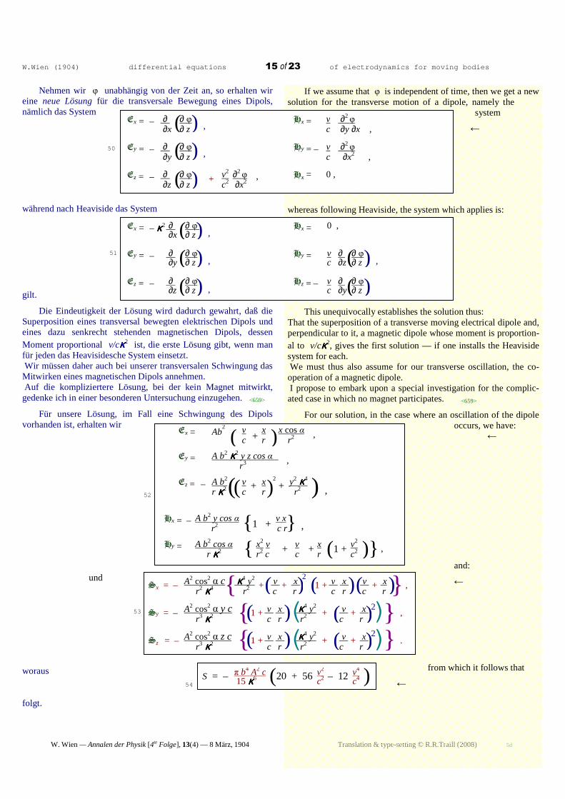
Nehmen wir φ unabhängig von der Zeit an, so erhalten wir eine neue Lösung für die transversale Bewegung eines Dipols, nämlich das System

während nach Heaviside das System

gilt.

Die Eindeutigkeit der Lösung wird dadurch gewahrt, daß die Superposition eines transversal bewegten elektrischen Dipols und eines dazu senkrecht stehenden magnetischen Dipols, dessen Moment proportional v/cκκκκ2 ist, die erste Lösung gibt, wenn man für jeden das Heavisidesche System einsetzt. Wir müssen daher auch bei unserer transversalen Schwingung das Mitwirken eines magnetischen Dipols annehmen. Auf die kompliziertere Lösung, bei der kein Magnet mitwirkt, gedenke ich in einer besonderen Untersuchung einzugehen. <659>

Für unsere Lösung, im Fall eine Schwingung des Dipols vorhanden ist, erhalten wir

und

woraus

folgt.

If we assume that φ is independent of time, then we get a new solution for the transverse motion of a dipole, namely the system

←

whereas following Heaviside, the system which applies is:

This unequivocally establishes the solution thus: That the superposition of a transverse moving electrical dipole and, perpendicular to it, a magnetic dipole whose moment is proportion-al to v/cκκκκ2, gives the first solution — if one installs the Heaviside system for each. We must thus also assume for our transverse oscillation, the co-operation of a magnetic dipole. I propose to embark upon a special investigation for the complic-ated case in which no magnet participates. <659>

For our solution, in the case where an oscillation of the dipole occurs, we have: ←

and:

←

from which it follows that

←

Ex = – ∂ ∂ φ Hx = v ∂2 φ ∂x ∂ z c ∂y ∂x , Ey = – ∂ ∂ φ Hy = – v ∂2 φ ∂y ∂ z c ∂x2 , Ez = – ∂ ∂ φ v2 ∂2 φ Hx = 0 , ∂z ∂ z c2 ∂x2

,

( ) ,

( ) ,

( ) +

S = – (20 + 56 – 12 ) π b4 A2 c v2 v4 15 κκκκ6 c2 c4

( ) A2 cos2 α c κκκκ4 y2 v x v x v x r

2 κκκκ4 r2 c r c r c r

A2 cos2 α y c v x κκκκ4 y2 v x r

3 κκκκ2 c r r2 c r

A2 cos2 α z c v x κκκκ4 y2 v x r

3 κκκκ2 c r r2 c r

Sx = – + + 1 + + , Sy = – 1 + + + , Sz = – 1 + + + .

( )2

( ) ( ) { }

( )

( )

( )2 ( )

( )2 ( )

{ }

{ }

50

52

53

54

51

Ex = – ∂ ∂ φ Hx = 0 , ∂x ∂ z Ey = – ∂ ∂ φ Hy = v ∂ ∂ φ ∂y ∂ z c ∂z ∂ z Ez = – ∂ ∂ φ Hz = – v ∂ ∂ φ ∂z ∂ z c ∂y ∂ z

( ) ,

( ) ,

( ) ,

( ) ,

( )

κκκκ2

Ex = Ab2 v x x cos α

c r r2 ,

Ey = A b2 κκκκ2 y z cos α r3

,

Ez = – A b2 v x 2 y2 κκκκ4 r κκκκ2 c r r2

Hx = – A b2 y cos α v x r

2 c r

Hy = A b2 cos α x2 v v x v2 r κκκκ2 r2 c c r c2

,

( + )

(( + ) + ) ,

{ 1 + } ,

{ + + (1 + )}



Here the emitted radiation itself will thus be infinite, as long as b/κκκκ remains finite.

Although now (according to the resolution of the problems for the case of an oscillation under the accepted presuppositions, and for all other associated cases, which can be handled through Fourier-series analysis), I choose to give another value for the func-tion F, which is not associated with any periodic precursor. I set φ thus:

The frame-of-thought which we previously set up for the oscillation, may be transferred unchanged to this new case.

Instead of the periodic travelling to-and-fro, here we have a once-only change from a negative to a positive value. If ε is very large, then we get the change in the arctg, from –π/2 to +π/2 in the vicinity of the zero-value of the relevant argument, and takes an asymptotic course for larger positive or negative values. <660>

If the size of ε is linked to the same conditions as those of b/κκκκ, then with a small enough amplitude, we can understand the proceedings as a once-only transverse or longitudinal impulse.

If we take the same system for the E und H as with the oscillation, and assume r to be infinitely large — then when we set: for the longitudinal impulse, the result will be:

If we now picture S as:

←

this will give us

←

For the transverse impulse we get:

and:

Here S will be infinite for v = c — for both the longitudinal and the transverse impulse — as long as ε remains finite.

2π2 A2 ε3 3 v2 15 κκκκ2 c2 . S = – (5 – )

Hier wird die Ausstrahlung selbst dann unendlich, wenn b/κκκκ endlich bleibt.

Obwohl nun nach der Erledigung des Problems für den Fall einer Schwingung unter den gemachten Voraussetzungen auch alle anderen hierher gehörenden Fälle durch Zerlegung nach Fourier-schen Reihen behandelt werden können, gebe ich doch einen anderen Wert der Funktion F, bei dem kein periodischer Vorgang eintritt. Ich setze - - - -

Die Betrachtungen, die wir für die Schwingung angestellt haben, lassen sich ohne weiteres auf diesen Fall übertragen.

Anstatt des periodischen Hin- und Hergehens haben wir hier nur einen einmaligen Wechsel von einem negativen zu einem positiven Wert. Ist ε sehr groß, so geht der Wechsel des arctg von –π/2 bis +π/2 in der Nähe des Nullwertes des Argumentes vor sich und verläuft für größere positive oder negative Werte asymptotisch. <660>

Ist die Größe von ε an dieselben Bedingungen geknüpft, wie die von b/κκκκ, so können wir bei genügend kleiner Amplitude den Vorgang als einen einmaligen transversalen oder longitudinalen Impuls auffassen.

Nehmen wir dieselben Systeme für die E und H wie bei der Schwingung und nehmen r als unendlich groß an, so ergibt sich, wenn wir - - - - setzen, für den longitudinalen Impuls

Bilden wir nun

so ergibt sich:

Für den transversalen Impuls erhalten wir

und

Hier wird S sowohl für den longitudinalen wie für den trans-versalen Impuls für v = c unendlich, solange ε endlich bleibt.74

A v x r c φ = arctg ε κκκκ2 c t – – r . ( )

v c ε κκκκ2c t – x – r = ε β ( )

4 ε6 β2 κκκκ4 c ρ2 A2 v x v x r

4 (1 + ε2 β2)4 c r c r

4 ε6 β2 κκκκ4 c ρ2 A2 κκκκ2 y v x r

4 (1 + ε2 β2)4 r c r

4 ε6 β2 κκκκ4 c ρ2 A2 κκκκ2 z v x r

4 (1 + ε2 β2)4 r c r

( ) ( ) Sx = – + 1 + , Sy = – · 1 + , Sz = – · 1 + .

( ) ( )

S = ∫dt ∫S dω , ∞

– ∞

4 ε6 β2 c A2 κκκκ4 y2 v x v x v x r2

(1 + ε2 β2)4 r2 c r c r c r 4 ε6 β2 c κκκκ2 y A2 v x κκκκ4 y2 v x r

3 (1 + ε2 β2)4 c r r2 c r

4 ε6 β2 c κκκκ2 z A2 v x κκκκ4 y2 v x r

3 (1 + ε2 β2)4 c r r2 c r

Sx = – + + 1 + + , Sy = – 1 + + + , Sz = – 1 + + +

( )2

{ }{ }{ }

( )2

( )2

{ }{ }

{ }{ }

S = – { 5 + 14 – } 2π2 A2 ε3 v2 3 v4 15 κκκκ4 c2 c4 .

55

56

57

58

59

60

61



Bei der Beurteilung dieses Ergebnisses für die Frage der Möglich-keit der Überlichtgeschwindigkeit muß berücksichtigt werden, daß wir die Strahlung über eine unendliche Zeit integriert haben. <661>

Für die Gültigkeit der Lösung genügt es, daß εa sehr klein ist. Die Strahlung, die ausgegeben wird, um bei Lichtgeschwindigkeit noch eine sehr kleine Strecke a während sehr langer Zeit mehr zurückzulegen, als die Lichtgeschwindigkeit selbst zurücklegt, wird daher unendlich sein. Daraus würde hervor gehen, daß bei Überschreitung der Licht-geschwindigkeit unendliche Arbeitsleistung verbraucht würde.

Die große Ausstrahlung bei transversaler Bewegung des Elek-trons würde zeigen, daß in der Nähe der Lichtgeschwindigkeit ein Elektron sich nicht mehr würde ablenken lassen.

Die durch transversale Bewegung eines Elektrons allein her-vorgerufene Strahlung gewinnen wir erst durch Benutzung der all-gemeineren Lösung, bei der die Mitwirkung eines Magneten fort-fällt. Ich gedenke dann auch auf die Vergleichung unserer Ergebnisse mit denen von Abraham11 näher einzugehen.

Obwohl nun die gewonnene Integration weit entfernt ist, eine vollständige Theorie des bewegten Elektrons zu ermöglichen, scheint sie mir einen großen Teil der wichtigen Fragen beantworten zu können. Mit einer Integration für beliebige veränderliche Geschwindigkeit-en ist insofern wenig gewonnen, als dann die augenblicklichen Vorgänge immer noch von allen vorausgegangenen Geschwindig-keiten abhängen. Das eigentliche Interesse wird sich daher zunächst vorzugsweise auf die Frage beschränken, was eintritt, wenn ein mit konstanter Geschwindigkeit bewegtes Elektron kleine Änderungen seines Weges erfährt.

Würzburg, Physikalisches Institut, November 1903.

(Eingegangen 30. November 1903.)

<662>

11 M. Abraham, loc.cit. [(1903), see footnote 6 for weblink: Ann. d. Phys. (s 4), 10. p.105-179. 1903. “Prinzipien der Dynamik des Elektrons”. RRT]

In reviewing this outcome for the question of the possibility of superluminary speed, it must be born in mind that we have integrat-ed the radiation over infinite time. <661>

For the solution to be valid, it suffices that εa should be very small. Concerning the emitted [electron] radiation: In order for it to travel at about the speed of light and outdistance light itself by a very small marginal distance of a during a very long journey-time, the [amount of] this radiation would thus have to be infinite. From that one would conclude, that any outstripping of the speed of light would require infinite work-energy.

The great radiation-emission via transverse motion of electrons would show, that, close to the speed of light, an electron would no longer be subject to reflection or refraction.

Concerning the radiation evoked solely through transverse motion of an electron: We first formulate that by using the general solution, from which is omitted the participation of any magnet. I therefore also propose getting closer in our comparison of our solutions to those of Abraham.11

Although now the achieved integration still falls far short of enabling a complete theory of the moving electrons, it seems to me that a major part of the important questions can be answered. With an integration for arbitrarily varied velocities, little is gained insofar as then the immediate events still always depend on all previous velocities. The real interest will thus next be preferentially limited to the question: What happens when a moving electron with constant speed experiences small changes in its direction?

Würzburg, Physikalisches Institut, November 1903.

(Submitted 30 November 1903.)

<662>



II. [2nd paper which follows immediately in the same volume] In my last investigation concerning the differential equations

of the electrodynamics for moving bodies, I had reported a method which supplies a general integral — a formulation for the case of a signal-source travelling with constant-but-arbitrary velocity, and emitting arbitrary electromagnetic disturbances. I had applied this integration method to longitudinal and transverse oscillations of an electric dipole. While [we] had found the first complete solution, the treatment of the transverse oscillations had remained incomplete in this way: The deep discussion of the achieved solution-system showed that, within it, the cooperation of a magnetic dipole must still be pre-supposed. Hence, pending further work, one cannot apply this solution to the especially-important problems of disturbances which are caused by electrons.

It is now the aim of this investigation to fill the mentioned gaps, and to deal with that solution for transverse oscillations which are not interacting with any magnet.

We achieve this special result through the tactic of identifying the magnet-participation (which simply superimposes itself), and subtracting it from the raw solution.

One gets the overall view over these relationships most simply when one temporarily eliminates dependence on time, and compar-es my two reported solutions for a transverse-moving dipole. <663>

These two systems may be stated as:

For the II case, one also gets (via superposition) the Heaviside solution for a single moving charge.

We now form the corresponding II system for a magnetic dipole whose axis is parallel to the y-axis, and whose moment contains the factor v/c. For this we get

II. [Zweiter Aufsatz, der folgt sofort im gleichen Band]

In meiner letzten Untersuchung über die Differentialgleich-ungen der Elektrodynamik für bewegte Körper hatte ich eine Methode angegeben, die ein allgemeines Integral für den Fall liefert, daß ein, beliebige elektromagnetische Störungen aussend-endes Zentrum mit konstanter, aber beliebig großer Geschwindig-keit bewegt wird. Diese Integrationsmethode hatte ich auf die longitudinalen und transversalen Schwingungen eines elektrischen Dipols angewendet. Während die ersteren vollständige Erledigung gefunden hatten, war die Behandlung der transversalen Schwingung insofern unvoll-ständig geblieben, als die genauere Diskussion des gewonnenen Lösungssystems zeigte, daß in ihr noch die Mitwirkung eines mag-netischen Dipols vorausgesetzt werden muß, so daß eine Anwend-ung dieser Lösung auf die besonders wichtigen Probleme von Störungen, die nur durch Elektronen hervorgerufen werden, nicht ohne weiteres zulässig ist.

Es ist nun der Zweck dieser Untersuchung, die erwähnte Lücke auszufüllen, und diejenige Lösung für transversale Schwing-ungen zu behandeln, bei der keine Mitwirkung eines Magneten stattfindet.

Wir gelangen zu dieser Lösung durch die Erwägung, daß wir die Beteiligung des Magneten, die sich einfach superponiert, von der Lösung abzuziehen haben.

Die Übersicht über diese Verhältnisse erhält man am einfach-sten, wenn man vorläufig Abhängigkeit von der Zeit ausschließt und die beiden bereits von mir angegebenen Lösungen für einen transversal bewegten Dipol vergleicht. <663>

Diese beiden Systeme lauteten:

(EI)

(EII)

Das mit II bezeichnete erhält man auch der Heavisideschen Lösung für eine bewegte Einzelladung durch Superposition.

Wir bilden nun das II entsprechende System für einen magnet-ischen Dipol, dessen Achse der y-Achse parallel ist, und dessen Moment den Faktor v/c enthält. Hierfür gewinnen wir

Ex = – ∂2 φ Hx = v ∂2 φ ∂x ∂z , c ∂y ∂x , Ey = – ∂2 φ Hy = – v ∂2 φ ∂y ∂z , c ∂x2 , Ez = – ∂2 φ v2 ∂2 φ Hz = 0 . ∂ z2 c2 ∂ x2 ,

+

Ex = – ∂2 φ Hx = 0 , ∂x ∂ z , Ey = – ∂2 φ Hy = v ∂2 φ ∂y ∂z , c ∂z2 , Ez = – ∂2 φ Hz = – v ∂2 φ ∂z2 , c ∂y ∂z .

κκκκ2

62

63



If we now add (EII) and (HII v/c), then we get (EI), which appears multiplied only by the factor of κκκκ2.

We designate this relation by the equation

so we can deduce a corresponding

from which

←

follows. <664>

We can use this relationship heuristically on the general case where φ depends on time — from the known solution-system I:

and do this in order to find a formulation for those cases where the contribution of a magnet is missing. We must first set up the corresponding system (provided with the factor v/c ) for the magnetic dipole. This appears as:

The subtraction of both sets of equations must then produce the sought-for result, and in that way we get:

(v/c HII)

Addieren wir nun (EII) und (HII v/c), so gewinnen wir (EI), das nur noch mit dem Faktor κκκκ2 multipliziert erscheint.

Bezeichnen wir diese Relation durch die Gleichung

so können wir eine entsprechende herleiten

→

woraus

→

folgt. <664>

Diese Beziehung können wir heuristisch verwerten, um für den allgemeinen Fall, wo φ von der Zeit abhängt, aus dem bekannten Lösungssystem I

.

dasjenige zu ermitteln, bei dem die Mitwirkung eines Magneten fehlt. Wir müssen zunächst das entsprechende, mit dem Faktor v/c versehene System für den magnetischen Dipol aufstellen. Diese lautet:

.

Die Subtraktion beider Gleichungssysteme muß dann das gesuchte liefern und wir erhalten somit

Ex = 0 , Hx = v ∂2 φ c ∂x ∂y , Ey = v2 ∂2 φ Hy = v ∂2 φ c2 ∂z ∂y , c ∂ y2 , Ez = – v2 ∂2 φ Hz = v ∂2 φ c2 ∂ y2 , c ∂z ∂y ,

κκκκ2

Ex = – ∂2 φ Hx = – 1 ∂2 φ – ∂2 φ ∂x ∂z , c ∂y ∂t ∂y ∂x Ey = – ∂2 φ Hy = 1 ∂2 φ – ∂2 φ ∂y ∂z , c ∂x ∂t ∂x2 Ez = ∂2 φ ∂2 φ Hz = 0 . ∂ x2 ∂ y2 ,

+

( v ) , ( v ) ,

69

64

EII + (v/c) HII = κκκκ2 EI ,

(v/c) HII + (v2/c2) EII + = (v/c)κκκκ2HI ,

EII (1 – v2/c2) = κκκκ2 (EI – (v/c)HI) ,

EII = EI – (v/c) HI

65

66

67

68

Ex = – v ∂2 φ ∂2 φ Hx = v ∂2 φ c2

∂z ∂t ∂z ∂x c ∂x ∂y , Ey = 0 , Hy = – v ∂2 φ ∂2 φ c ∂x2 ∂z2 Ez = – v ∂2 φ ∂2 φ Hz = v ∂2 φ c2

∂x ∂t ∂x2 c ∂z ∂y ,

( ) ,

– ( v ) , +

– ( v ) ,

70 Hy here re- sequenced

(…)v/c to v/c(…) to aid uniformity

[RRT 2008]



Indeed this system now performs all that is required. For v = 0 , it becomes the Hertz-solution-set for an oscillating dipole. For ∂ φ/∂t = 0 , it becomes the system one gets from the Heaviside solution of a moving charge for a transversely oscillating moving electrical dipole.

We can use this solution to compute the radiation of a transverse oscillating dipole.

We set again

←

<665>

then we get:

Furthermore there arises

and

←

integrates over an infinitely large ellipsoid

←

.

Dieses System leistet nun in der Tat alles verlangte. Es geht für v = 0 in das Hertzsche Lösungssystem für einen schwingenden Dipol, für ∂ φ/∂t = 0 in das System über, das man aus der Heavisideschen Lösung einer bewegten Ladung für einen transversal bewegten elektrischen Dipol erhält.

Wir können diese Lösung benutzen, um die Strahlung eines transversal schwingenden Dipols zu berechnen.

Setzen wir wieder

<665>

dann erhalten wir

Ferner ergibt sich

und

→

über ein unendlich großes Ellipsoid integriert

→

71

Ex = – ∂2 φ v ∂2 φ Hx = – 1 ∂2 φ ∂x ∂z c2 ∂z ∂t , c ∂y ∂t , Ey = – ∂2 φ Hy = 1 ∂2 φ + v ∂2 φ ∂y ∂z , c ∂x ∂t c ∂z2 , Ez = ∂2 φ ∂2 φ v ∂2 φ Hz = – v ∂2 φ ∂ x2 ∂ y2 c2 ∂x ∂t , c ∂z ∂y .

κκκκ2 –

φ = (A/r) cos(b/κκκκ) (κκκκ2 c t – (v/c) x – r) ,

r2 = x2 + (y2 + z2) κκκκ2 κκκκ2 = 1 – v2/c2 ,

α = (b/κκκκ) (κκκκ2 c t – (v/c) x – r) ,

72

κκκκ2 + +

Ex = – ∂ ∂ φ v ∂ φ ∂z ∂ x c2 ∂ t Ex = A x z Hx = – A y r r

2 r r

Ey = A y z Hy = A x v v z2 r r

2 r r c c r2 ,

Ez = – A x v x x2 y2 Hz = A v y z r r c r r2 , r c r2 .

κκκκ2 + ( ) , b2κκκκ2 cos α ,

b2κκκκ2 cos α ,

b2 cos α + + (( ) )

b2κκκκ2 cos α ,

b2 cos α + – κκκκ2 (( ) )

b2 cos α κκκκ2

73

[ ←ambiguous!]

Sx = – A2b4c x2 y2 v x x x v v κκκκ2z2 y2 z2 v r

2 r

2 c r r r c c r2 r4 c . Sy = – A2b4c v z2 x y y κκκκ2 κκκκ2y2 v x x r

2 c r4 r r2 c r r .

Sz = – A2b4c x4 y2 z z x x v v z3 x r

2 r

3 r2 r c c r4 .

{( ( ) ) ( ) } cos2 α + + + – + κκκκ4

cos2 α – κκκκ4 + + + { ( ( ) )} cos2 α + κκκκ2 + – κκκκ4 { ( ) }

S = ∫ dt ∫ S dω

= – 20 – 4 ,

2 π b κκκκ c

b κκκκ c 2 π

π b4 A3 c v2 15κκκκ2 c2

{ }

74

75

76



and for the case that we replace the function ← , assuming instead ← <666> The emitted radiation is thus not infinite, for finite values of ε or of b/κκκκ — also for v = c . However it does become infinite if b κκκκ remains finite for v = c.

Finite values of b κκκκ mean finite values of the wave-number [and hence frequency]. For these the radiant emission is infinite on reaching the speed of light. Electrons approaching the speed of light are thus no longer divertable.

If we compare our results ← and ←

with those of Abraham,21 then a disagreement shows up in the dependency on v/c. Abraham opts for the v/c -dependent factor 1/κκκκ2 in the one, and for 1 in the other. For small values of v/c they are:

1 + v2/c2 and 1 ,

while they result in

1 + (7/5) v2/c2 and 1 + (4/5) v2/c2

on using our values.

Since Abraham did not specify his direction-vectors, it is not possible to trace the reason for this discrepancy.

Finally I would especially like to refer again to the circum-stance previously mentioned in this investigation — that the introduction of a magnetic pole was necessary to protect the integrity of the solution. Although now in the symmetrical structure of the Maxwell equat-ions, the magnetic components appear just as legitimate as the electric, there is nevertheless the especially important question of whether real magnetic elementary quanta are to be assumed. In the theory so far, there is the tendency to ascribe only the electrical elementary-components to the reciprocal effect between aether and matter, <667> and to associate the magnetic characteristics of bodies to their motion.22 According to this, magnetic quanta are only fictions — an analogy with Ampère’s double magnetic layer as an enclosing surface around a linear conductor.

und für den Fall, daß wir anstatt

→

die Funktion

→

annehmen

<666>

Die Ausstrahlung ist also für endliche Werte von ε oder von b/κκκκ auch für v = c nicht unendlich. Sie wird aber unendlich, wenn b κκκκ endlich bleibt für v = c.

Endliche Werte von b κκκκ bedeuten endliche Werte der Schwingungszahl. Für diese ist die Ausstrahlung unendlich bei Erreichung der Licht-geschwindigkeit. Elektronen in der Nähe der Lichtgeschwindigkeit sind also nicht mehr ablenkbar.

Wenn wir unsere Ergebnisse →

und →

mit den Ergebnissen von Abraham21 vergleichen, so zeigt sich in der Abhängigkeit von v/c ein Mangel an Übereinstimmung. Hr. Abraham findet für den von v/c abhängigen Faktor 1/κκκκ2 im einen, und 1 im anderen Falle. Für kleine Werte von v/c sind sie

1 + v2/c2 und 1 ,

während sie sich aus unseren Werten

1 + (7/5) v2/c2 und 1 + (4/5) v2/c2

ergeben.

Da Hr. Abraham seine Richtungen nicht mitgeteilt hat, so ist es nicht möglich, dem Grund dieser Verschiedenheit nachzuspüren.

Schließlich möchte ich noch auf den in diesen Untersuchungen hervorgetretenen Umstand besonder hinweisen, daß die Einführung magnetischer Pole notwendig war, um die Eindeutigkeit der Lös-ungen zu wahren. Obwohl nun in dem symmetrischen Bau der Maxwellschen Gleichungen die Existenz magnetischer Quanta ebenso wie die elektrischer ganz gleichberechtigt erscheint, so ist doch die Frage von besonderer Wichtigkeit, ob wirkliche magnetische Elementar-quanten anzunehmen sind. In den bisherigen Theorie tritt die Neigung hervor, die Wechsel-wirkung zwischen Äther und Materie nur den elektrischen Elem-entarquanten zuzuschreiben und die<667> magnetischen Eigen-schaften der Körper auf Bewegung dieser zurückzuführen.22 Magnetische Quanten sind hiernach nur Fiktionen nach Analogie der Ampèreschen magnetischen Doppelschicht auf einer von einem linearen Stromleiter umschlossenen Fläche.

21 M. Abraham, Ann. d. Phys. 10. p.105. 1903. [(series 4); “Prinzipien der Dynamik des Elektrons”, pp.105-179.

Follow link from www.weltderphysik.de/de/3001.php?bd315 for a facsimile of the original. RRT]

22 F. Richarz, Ber. d. Münchener Akad. 24. 1894.

S = – 5 – . 2 π2 A2 ε3 v2 15 c2

( )

cos (b/κκκκ) (κκκκ2ct – (v/c) x – r)

↓ arctg ε (κκκκ2ct – (v/c) x – r)

77

78

S = – 5 – . 2 π2 A2 ε3 v2 15 c2

( )

Se = – 20 – 12

St = – 20 – 4

( )

π b4 A2 c v2 15 κκκκ4 c2

π b4 A2 c v2 15 κκκκ2 c2

( )

79

80



This view is supported by the fact that there is no isolated positive or negative magnetism.

Now the magnetic quantum of the magnetic dipoles introduced by us is likewise zero, and we could set up the statement that these dipoles are likewise only fictitious — to represent a special arrangement of magnetic field lines which are due to the movement of the electrical dipole. Here however the arbitrariness in the alternative interpretation of electrical and magnetic dipoles (which are quite equi-valid in the theory) is risky. So too is the necessity to abandon the self-consistency of the solution; since if we regard the magnetic dipoles as only fictitious, and if the two solutions considered for a transversally-moving electric dipole are equally valid, that might be extremely awkward for the theoret-ical treatment. If on the other hand we assume the possibility of the existence of magnetic quanta (which operate directly on the aether quite analogously to electrical quanta), then both solutions are to be regarded as different, because it must naturally make a difference whether magnetic effects still really exist anywhere beyond the electric dipole.

Würzburg, Physikalisches Institut, January 1904.

(Received 7. January 1904.)

<668>

Unterstützt wird diese Auffassung durch die Tatsache, daß es isolierten positiven oder negativen Magnetismus nicht gibt.

Nun ist das magnetische Quantum der von uns eingeführten magnetischen Dipole ebenfalls Null und wir könnten die Behaupt-ung aufstellen, daß diese Dipole ebenfalls nur fingiert sind, um eine besondere Anordnung magnetischer Kraftlinien, die von der Bewegung des elektrischen Dipols herrühren, darzustellen. Bedenklich ist hierbei aber die Willkür in der verschiedenen Auf-fassung des elektrischen und magnetischen Dipols, die in der Theorie ganz gleichberechtigt auftreten, ferner die Notwendigkeit, die Eindeutigkeit der Lösungen aufzugeben. Denn wenn wir die magnetischen Dipole nur als fingiert ansehen, dann sind die beiden betrachteten Lösungen für einen transversal bewegten elektrischen Dipol gleich berichtigt, was für die theoret-ische Behandlung äußerst mißlich sein dürfte. Nehmen wir dagegen die Möglichkeit der Existenz magnetischer Quanten, die ganz analog den elektrischen direkt auf den Äther einwirken, an, so sind sie beiden Lösungen als verschieden anzu-sehen, weil es natürlich einen Unterschied machen muß, ob außer dem elektrischen Dipol noch ein wirklich existierender magnet-ischer mitwirkt oder nicht.

Würzburg, Physikalisches Institut, Januar 1904.

(Eingegangen 7. Januar 1904.)

<668>

INHALT / CONTENTS

Über die Differentialgleichungen der Elektrodynamik für bewegte Körper;..................................................................................................... 2

1. Beziehung der Lorentzschen Gleichungen zu denen für ruhende Körper................................................................................................. 5 2. Geschwindigkeit der Ausbreitung der Störungen ..................................................................................................................................... 8 3. Einfluss der Bewegung auf die Strahlung................................................................................................................................................. 9

II. [Zweiter Aufsatz, der folgt sofort im gleichen Band] .................................................................................................................................. 18 INHALT ............................................................................................................................................................................................. 22

Consolidated References (von Fussnoten)................................................................................................................................................ 23 On the differential equations of the electrodynamics for moving bodies; ......................................................................................................... 2

1. Relationship between the Lorentz equations and those for resting bodies................................................................................................ 5 2. Speed for the dissemination of a disturbance............................................................................................................................................ 8 3. Influence of motion on the radiation......................................................................................................................................................... 9

II. [2nd paper which follows immediately in the same volume]........................................................................................................................ 18 CONTENTS ............................................................................................................................................................................................22

Consolidated References (from the various footnotes)............................................................................................................................ 23



Consolidated References (from the various footnotes)

— here listed in Alphabetical order. (Note: The same list appears in Chronological order for the Cohn papers: www.ondwelle.com/Cohn.pdf ) ex foot

(Cohn) -notes: (Wien)

author date description

6, 11, I2 Abraham, M. (1903). Annalen der Physik (series/Folge 4) 10, 105-179. “Principien der Dynamik des Elektrons”.

For a facsimile of the original, follow the “Band 315” link from www.weltderphysik.de/de/3001.php 3, 6 Cohn, E. (1900a) Das elektromagnetische Feld, Leipzig 1900, — [insbesondere / especially p.279f.] — [abbrev. as „elm. Feld“ ]

4 Cohn, E. (1900b) Archives néerlandaises des scienceces exactes et naturelles (2), 5. (Lorentz-Jubelband) p.516-523. “Über die Gleichungen der Elektrodynamik für bewegte Körper”. [die Gleichungen bereits in:…]

L 4, 1(self)

Cohn, E. (1902a) Annalen der Physik (series/Folge 4) 7, 29-56. “Ueber die Gleichungen des elektromagnetischen Feldes für bewegte Körper” — The digitized and translated English+German text is at www.ondwelle.com/Cohn.pdf [↓]

K Cohn, E. (1904, May 10)

Annalen der Physik (series/Folge 4), 14(6), 208. [Brief note in reply to (Wien, 1904 March), in prev. vol.(13)] ‘Antikritisches zu Hrn. W. Wiens „Differentialgleichungen der Elektrodynamik für bewegte Körper“ ’ The digitized English+German text is at the end of www.ondwelle.com/Cohn,pdf [URL corrected 29/10/2012]

C Einstein, A. (1905 Sep 26)

Annalen der Physik (series/Folge 4), 17(10), 891-921. “Zur Elektrodynamik bewegte Körper”. [This is the landmark paper which initiated Special Relativity Theory]

E Euler, L. (1766/1808) “Reserches sur l’intégration de l’équation (ddz/dt2) = aa(ddz/dx2) + b/x •(dz/dx) + (c/xx).z ” — [Euler’s] Opera Omnia (series 1), 23, 42-73.

A Fizeau, H. (1859-Dec) Annales de Chimie et de Physique, 57, 385-404. “Sur les hypothèses relatives à l’éther lumineux”. http://gallica.bnf.fr/ark:/12148/bpt6k347981/f381.table [Originally presented to the Parisian Academy of Sciences, 29 Sep 1851]

I, G Fizeau, H. (1860-Apr) Philosophical Magazine (ser.4), 19, 245-260. “On the effect of the motion of a body upon the velocity with which it is traversed by light”. — English translation of Fizeau (1859) which also includes an editorial account of a second experiment. Facsimile available at http://wbabin.net/fizeau1.pdf

2 [v45 636, 881]

D, H Heaviside, O. (1900-1902) “Electromagnetic Theory — CXII-CXXVI” The Electrician, 44 (#18: 23 Feb 1900), 615- , continuing in episodes to 48 (Jan 1902?), -221; republished (with added subheadings) as Chapter 9 “Waves from moving sources” in his Electromagnetic Theory , vol. III (1912).

D Heaviside, O. (1902 Feb 14 – June 6). + Sequel:

“Electromagnetic Theory — CXXVII-CXXVIII” The Electrician; then continued in Nature (Oct 30 (p6), Nov 6 (p32); 1903 Jan 1 (p202), 1904 Jan 28 (p293), 1904 Feb 11 (p342), 1903 Jan 29 (p297)... — republished in that order, as Chapter 10 “Waves in the Ether” in his Elec.Mag.Theory, III (1912).

7 Helmholtz, H.v. (1882-) Wissenschaftliche Abhandlungen, vol.3. Leipzig. — p. 531 f.

9, G Hertz, H.R. (1889 Jan) Annalen der Physik (series 2 [Ed. by Wiedemann] ). 36(1), 1-22, + Tafel I: Figs.1-6.). “Die Kräfte electrischer Schwingungen, behandelt nach der Maxwell’schen Theorie” — [Dipole oscillating in the x-direction — including Hertz’s famous pre-radio experiment]

A Hertz, H.R. (1890a) Annalen der Physik und Chimie (2nd series [Ed. by Wiedemann] ), 40, 577-624. “Ueber die Grundgleichungen der Electrodynamik für ruhende Körper”. — [Aus den Gött.Nachr. vom 19. März 1890.] — On the basic equations for the electrodynamics of stationary bodies.

B, H 2 Hertz, H.R. (1890b) Annalen der Physik (series 2: [Ed. by Wiedemann) ]. 41. p.369-399. “Ueber die Grundgleichungen der Elektrodynamik für bewegte Körper”]— On the basic equations for the electrodynamics of moving bodies.

7 Hertz, H.R. (1892) Untersuchung über die Ausbreitung der elektrischen Kraft,. Joh.A.Barth: Leipzig. — p. 284-

B Kaufmann,W. (1902) Physikalische Zeitung, 4, p.54-57 “Die elektromagnetische Masse des Elektrons” [as a function of velocity] B Kaufmann,W. (1903) Gött.Nachrichtungen Math. phys. Kl. B Kaufmann,W. (1906) Annalen der Physik (series 4), 19, 487- A Lerche. I. (1977 Dec) “The Fizeau Effect: Theory, experiment, and Zeeman’s measurements”. Amer. J. Phys., 45(12), 1154-1163. 5 Lorentz, H.A. (1892) Théorie électrique de Maxwell et son application aux corps mouvants p.119. Leiden.

5 1, 8, 10 Lorentz, H.A. (1895/1935) Versuch einer Theorie der elektrischen und optischen Erscheinungen in bewegten Körpern. Leiden. / “Search for a theory of electrical and optical phenomena in moving bodies” [Also in his Collected Papers, vol. 5, pp.1-138. Martinus Nijhoff: The Hague. ].

B, C Lorentz, H.A. (1904) Proc.Acad.Sciences Amsterdam, 6. 5, F Lorenz, L. (1867) Annalen der Physik (series 1, [alias “Pogg.Ann.”: Ed. by Poggendorff] ). 131. p.243-263. G 3 Michelson, A.A.

& E.W.Morley (1886 May) American J. Science (series 3), 31, 377-386. “Influence of Motion of the Medium on the Velocity of Light”. —

repeating the famous experiment by H.Fizeau (1859).I and repeated again later by Zeeman (1914-).

C Michelson, A.A. & E.W.Morley

(1887 Nov). American Journal of Science, (series 3). 34, 333-345. — Also in: Phil. Mag. and Journal of Science, (5th series). 24, 449-463. — “On the relative motion of the Earth and the luminiferous ether”

7 Poincaré, H. (1900). Festschrift für H.A.Lorentz, p.252. Leiden.

12 Richarz, F. (1894). Sitzungsberichte der Münchener Akademie, 24.

1 Walker, G.T. (1900) Aberration and the electromagnetic field (Cambridge, 1900).

8 C, F Wien, W. (1904,

Mar 8)a Annalen der Physik (series/Folge 4), 13(4), 663-668. “Über die Differentialgleichungen der Elektrodynamik für bewegte Körper” [Part 1] — see http://www.ondwelle.com/Wien.pdf for digitized and translated English+German version. For a facsimile of the original, follow the “Band 318” link from www.weltderphysik.de/de/3001.php

8 Wien, W. (1904, Mar 8)b

Annalen der Physik (series/Folge 4), 13(4), 641-662. “Über die Differentialgleichungen der Elektrodynamik für bewegte Körper” [Part 2] — see last part of http://www.ondwelle.com/Wien.pdf for digitized and translated English+German version.

(G) (A) Zeeman, P. (1914) Proc. Kon. Acad. van Weten, 17(..), 445-451. “Fresnel’s coefficient for light of different colours. (First part)”. http://www.digitallibrary.nl/proceedings/search/detail.cfm?pubid=1708&view=image&startrow=1

(G) (A) Zeeman, P. (1915) Proc. Kon. Acad. van Weten, 18(..), 398-408. “Fresnel’s coefficient for light of different colours. (Second part)”. http://www.digitallibrary.nl/proceedings/search/detail.cfm?pubid=1847&view=image&startrow=1

�

�

In t

he

pres

ent

do

cum

ent

on the differential equations of the electrodynamics for ... fileon the differential equations of...

Documents