chapter 6 – stream hydraulics

Part 654 Stream Restoration Design National Engineering Handbook

Chapter 6 Stream Hydraulics

United StatesDepartment ofAgriculture

Natural ResourcesConservationService

(210–VI–NEH, August 2007)

Issued August 2007

The U.S. Department of Agriculture (USDA) prohibits discrimination in all its programs and activities on the basis of race, color, national origin, age, disability, and where applicable, sex, marital status, familial status, parental status, religion, sexual orientation, genetic information, political beliefs, reprisal, or because all or a part of an individual’s income is derived from any public assistance program. (Not all prohibited bases apply to all programs.) Persons with disabilities who require alternative means for communication of program information (Braille, large print, audiotape, etc.) should contact USDA’s TARGET Center at (202) 720–2600 (voice and TDD). To file a com-plaint of discrimination, write to USDA, Director, Office of Civil Rights, 1400 Independence Avenue, SW., Washing-ton, DC 20250–9410, or call (800) 795–3272 (voice) or (202) 720–6382 (TDD). USDA is an equal opportunity pro-vider and employer.

Advisory Note

Techniques and approaches contained in this handbook are not all-inclusive, nor universally applicable. Designing stream restorations requires appropriate training and experience, especially to identify conditions where various approaches, tools, and techniques are most applicable, as well as their limitations for design. Note also that prod-uct names are included only to show type and availability and do not constitute endorsement for their specific use.

Part 654National Engineering Handbook

Stream HydraulicsChapter 6

Cover photo: Stream hydraulics focus on bankfull frequencies, veloci-ties, and duration of flow, both for the current condition, as well as the condition anticipated with the project in place. Effects of vegetation are considered both in terms of protec-tion of the bank materials, as well as on changes in hydrau-lic roughness.

(210–VI–NEH, August 2007) 6–i

Contents


654.0600 Purpose 6–1

654.0601 Introduction 6–1

(a) Hydraulics as physics .....................................................................................6–1

(b) Hydraulics as empiricism ...............................................................................6–2

645.0602 Channel cross-sectional parameters 6–3

654.0603 Dimensionless ratios 6–4

(a) Froude number ................................................................................................6–4

(b) Reynolds number ............................................................................................6–4

654.0604 Continuity 6–5

624.0605 Energy 6–6

654.0606 Momentum 6–7

654.0607 Specific force 6–8

654.0608 Stream power 6–9

654.0609 Hydraulic computations 6–9

(a) Uniform flow ....................................................................................................6–9

(b) Determining normal depth ...........................................................................6–10

(c) Determining roughness coefficient (n value) ............................................6–12

(d) Friction factor ................................................................................................6–17

(e) Accounting for velocity distributions in water surface profiles ..............6–17

(f) Determining the water surface in curved channels ..................................6–18

(g) Transverse flow hydraulics and its geomorphologic effects ...................6–19

(h) Change in channel capacity .........................................................................6–24

654.0610 Water surface profile calculations 6–25

(a) Steady versus unsteady flow ........................................................................6–27

(b) Backwater computational models ..............................................................6–28

654.0611 Weir flow 6–29

654.0612 Hydraulic jumps 6–30

654.0613 Channel routing 6–32

(a) Movement of a floodwave ............................................................................6–32

(b) Hydraulic and hydrologic routing ...............................................................6–32

(c) Saint Venant equations .................................................................................6–33

(d) Simplifications to the momentum equation ...............................................6–33

654.0614 Hydraulics input into the stream design process 6–35

(a) Determining project scope and level of analysis .......................................6–35

(b) Accounting for uncertainty and risk ...........................................................6–36

6–ii (210–VI–NEH, August 2007)



Tables Table 6–1 Froude numbers for types of hydraulic jumps 6–30

Table 6–2 Project dimensions by type and stage of project 6–35

Table 6–3 Scope of hydraulic analyses by project type 6–35

Figures Figure 6–1 Channel cross-sectional parameters 6–3

Figure 6–2 Specific energy vs. depth of flow 6–6

Figure 6–3 Problem cross section 6–10

Figure 6–4 HEC–RAS screen shot for uniform flow computation 6–11

Figure 6–5 Cross-sectional dimensions 6–12

Figure 6–6 Looking upstream from left bank 6–13

Figure 6–7 Looking downstream on right overbank 6–13

Figure 6–8 Sand channel cross section 6–14

Figure 6–9 Plot of flow regimes resulting from stream power 6–15vs. median fall diameter of sediment

Figure 6–10 General bedforms for increasing stream power 6–16

Figure 6–11 Flow velocities for a typical cross section 6–18

Figure 6–12 Spiral flow characteristics for a typical reach 6–20

Figure 6–13 Flow characteristics for a typical reach 6–20

Figure 6–14 Channel centerline at centroid of flow 6–22

Figure 6–15 Point bar development 6–23

Figure 6–16 Seasonal hydrograph 6–24

Figure 6–17 Standard step method 6–25

Figure 6–18 Problem determinations for determination of log 6–26weir

6–iii(210–VI–NEH, August 2007)



Figure 6–19 Profile for crest of log weir problem 6–26

Figure 6–20 Determination of jump length based on upstream 6–31Froude number

Figure 6–21 Parameters involved with modeling a hydraulic 6–31jump

(210–VI–NEH, August 2007) 6–1


654.0600 Purpose

Human intervention in the stream environment, espe-cially with projects intended to restore a stream eco-system to some healthier state, must fully consider the stream system, stream geomorphology, stream ecol-ogy, stream hydraulics, and the science and mechanics of streamflow. This chapter provides working profes-sionals with practical information about hydraulic parameters and associated computations. It provides example calculations, as well as information about the role of hydraulic engineers in the design process.

The hydraulic parameters used to evaluate and quan-tify streamflow are described in this chapter. The applicability of the various hydraulic parameters in planning and design in the stream environment is presented. The complexity of streamflow is addressed, as well as simplifying assumptions, their validity, and consequences. Guidance is provided for determining the level of analysis commensurate with a given proj-ect’s goals and the associated hydraulic parameters. Finally, a range of analytical tools is described, the application of which depends on the complexity of the project.

Stream hydraulics is a complex subject, however, and this chapter does not provide exhaustive coverage of the topic. Readers are encouraged to supplement this information with the many good references that are available.

654.0601 Introduction

Stream hydraulics is the combination of science and engineering for determining streamflow behavior at specific locations for purposes including solving prob-lems that generally originate with human impacts. A location of interest may be spatially limited, such as at a bridge, or on a larger scale such as a series of chan-nel bends where the streambanks are eroding. Flood depth, as well as other hydraulic effects, may need to be determined over long stretches of the channel.

An understanding of flowing water forms the basis for much of the work done to restore streams. The disci-pline of hydrology involves the determination of flow rates or amounts, their origin, and their frequency. Hydraulics involves the mechanics of the flow and, given the great power of flowing water, its affect on bed, banks, and structures.

A stream is a natural system that constantly adjusts itself to its environment and participates in a cycle of action and reaction. These adjustments may be gradual, less noticeable, and long term, or they may be sudden and attention grabbing. The impacts causing a stream to react may be natural, such as a rare, intense rainfall, or human-induced, such as the straighten-ing of a channel or filling of a wetland. However, the reaction of a stream to either kind of change may be more than localized. A stream adjusts its profile, slope, sinuosity, channel shape, flow velocity, and boundary roughness over long sections of its profile in response to such impacts. After an impact, a stream may restore a state of equilibrium in as little as a week, or it may take decades.

(a) Hydraulics as physics

Stream characteristics are derived from the basic physics of flowing water. Fluid mechanics is an old science with well-established physical relationships. Typically, simple empirical equations are used that do not account for all the variability that occurs in the flow. An example is Bernoulli’s equation for balanc-ing flow depth, velocity, and pressure. In this case, the flow must be considered steady. If it is important to assess how flow depth, velocity, and/or pressure

6–2 (210–VI–NEH, August 2007)



change over time, Bernoulli’s equation by itself will not be sufficient.

The assumption that flow velocity is generally down-stream in direction is also a common simplification in the analysis of streamflow. Real streams have many eddies where the flow circulates horizontally. Streams also have areas of upwelling, roiling, and vertical circulation. While designers commonly make use of an average velocity at a given cross section, the actual velocities in the plane of a cross section vary markedly from top to bottom, side to side, and in direction, vary-ing with time and three-dimensional space.

Water surface profile analyses generally assume a con-stant flow elevation across a given cross section. Real streams, however, super-elevate their water surfaces in curved channel sections and may set up significant surface wave patterns that defy prediction. Finally, hy-draulic analyses often assume that water flows against a fixed boundary. Real streams actually readjust their bed and banks constantly, move significant amounts of sediment, and transport unpredictable amounts of natural or humanmade debris.

It is, therefore, important to understand the limitations and restrictions of any equations before using them to obtain necessary information.

(b) Hydraulics as empiricism

Although thoroughly founded in physics, many hydrau-lic relationships require empirical coefficients to ac-count for unmeasured or estimated processes. One of the parameters that has a significant influence on hy-draulic calculations is surface roughness, in the form of Manning’s n value, the Chézy C, or the Darcy-Weis-bach friction factor. While the Darcy-Weisbach friction factor is generally considered to be more theoretically based, Manning’s n is more commonly used for most stream design and restoration analysis. Roughness is a function of many stream physical properties includ-ing bed sediment size, vegetation, channel sinuosity, channel irregularity, and suspended sediment load. As a result, many of the estimates have inherent degrees of empiricism in their estimate.

Sediment transport also requires empirical input. Sedi-ment particles vary in size and properties, from tiny silt particles that adhere to large boulders, sometimes

redirecting a stream and sometimes transported down-stream. Sediment transport is influenced by velocity vectors near the water/sediment boundary, and these bed velocities may not be well predicted by an average cross-sectional velocity. Many of the analytical sedi-ment predictive techniques include many empirical estimates of specific parameters. More information on the analytical, as well as empirical approaches to sedi-ment transport, is provided in other chapters of this handbook. More information on sedimentation analy-sis is provided in NEH654.09 and NEH654.13.

6–3(210–VI–NEH, August 2007)



645.0602 Channel cross-sectional parameters

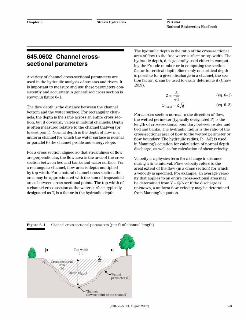
A variety of channel cross-sectional parameters are used in the hydraulic analysis of streams and rivers. It is important to measure and use these parameters con-sistently and accurately. A generalized cross section is shown in figure 6–1.

The flow depth is the distance between the channel bottom and the water surface. For rectangular chan-nels, the depth is the same across an entire cross sec-tion, but it obviously varies in natural channels. Depth is often measured relative to the channel thalweg (or lowest point). Normal depth is the depth of flow in a uniform channel for which the water surface is normal or parallel to the channel profile and energy slope.

For a cross section aligned so that streamlines of flow are perpendicular, the flow area is the area of the cross section between bed and banks and water surface. For a rectangular channel, flow area is depth multiplied by top width. For a natural channel cross section, the area may be approximated with the sum of trapezoidal areas between cross-sectional points. The top width of a channel cross section at the water surface, typically designated as T, is a factor in the hydraulic depth.

The hydraulic depth is the ratio of the cross-sectional area of flow to the free water surface or top width. The hydraulic depth, d, is generally used either in comput-ing the Froude number or in computing the section factor for critical depth. Since only one critical depth is possible for a given discharge in a channel, the sec-tion factor, Z, can be used to easily determine it (Chow 1959).

Z = A

d (eq. 6–1)

Q Z gcritical = (eq. 6–2)

For a cross section normal to the direction of flow, the wetted perimeter (typically designated P) is the length of cross-sectional boundary between water and bed and banks. The hydraulic radius is the ratio of the cross-sectional area of flow to the wetted perimeter or flow boundary. The hydraulic radius, R= A/P, is used in Manning’s equation for calculation of normal depth discharge, as well as for calculation of shear velocity.

Velocity is a physics term for a change in distance during a time interval. Flow velocity refers to the areal extent of the flow (in a cross section) for which a velocity is specified. For example, an average veloc-ity that applies to an entire cross-sectional area may be determined from V = Q/A or if the discharge is unknown, a uniform flow velocity may be determined from Manning’s equation.

Figure 6–1 Channel cross-sectional parameters (per ft of channel length)

Depth (dmax)

Thalweg(lowest point of the channel)

Wettedperimeter (P)

Top width(T)

Cross-sectionalarea(A)

6–4 (210–VI–NEH, August 2007)



Another useful formulation is critical velocity, which is average flow velocity at critical depth, and is calcu-lated from equation 6–3:

V gdcr cr= (eq. 6–3)

where:V

cr = critical velocity

g = gravitational accelerationd

cr = critical depth

Determining the state of flow is a matter of determin-ing whether the velocity is greater than critical veloc-ity V

cr (supercritical flow) or less than critical velocity

Vcr

(subcritical flow).

Conveyance is a measure of the flow-carrying capac-ity of a cross section which is directly proportional to discharge. Conveyance, typically designated K, may be expressed from Manning’s equation (without the slope term) as:

K AR n

=1 486 2

3.

(eq. 6–4a)

or

KQ

S= (eq. 6–4b)

where:A = flow area (ft2)R = hydraulic radius (ft)Q = flow rate (ft3/s)S = slope, dimensionless

In backwater calculations, change in conveyance from cross section to cross section is a useful way to de-termine the adequacy of section spacing in a stream reach. Within a cross section, conveyance may be used to compare channel and overbank flow carrying capac-ity.

654.0603 Dimensionless ratios

Dimensionless ratios (also referred to as dimension-less numbers) are used to provide information on flow condition. The units of the variables used in the equa-tion for a dimensionless ratio are such that they can-cel. The two most commonly used ratios are Froude and Reynolds numbers. Being dimensionless allows their application to be made across a variety of scales.

(a) Froude number

The Froude number is a dimensionless ratio, relat-ing inertial forces to gravitational forces. The Froude number represents the effect of gravity on the state of flow in a stream (Chow 1959). This useful number was derived by a nineteenth century English scientist, Wil-liam Froude, who studied the resistance of ships being towed in water. He observed wave patterns along the hull of a moving ship and found that the same number of waves would occur as long as the ratio of the ship’s speed to the square root of its length were the same. Applied in hydraulics, the length is replaced by hy-draulic depth, as shown in equation 6–5.

FV

gd= (eq. 6–5)

where:V = velocity (ft/s)g = acceleration due to gravity (32.2 ft/s2)d = flow depth (ft)

If the Froude number is less than one, gravitational forces dominate and the flow is subcritical, and if greater than one, inertial forces dominate and the flow is supercritical. The Froude number is used to determine the state of flow, since, for subcritical flow the boundary condition is downstream, and for super-critical flow it is upstream. When the Froude number equals one, the flow is at the critical state.

(b) Reynolds number

The Reynolds number is also a dimensionless ratio, relating the effect of viscosity to inertia, used to deter-mine whether fluid flow is laminar or turbulent (Chow 1959). The Reynolds number relates inertial forces to

6–5(210–VI–NEH, August 2007)



viscous forces and was derived by a nineteenth centu-ry English scientist, Osborne Reynolds, for use in wind tunnel experiments.

Inertia is represented in equation 6–6 by the product of velocity and hydraulic radius, divided by the kine-matic viscosity of water, with units of length squared per time. For turbulent flow Re>2000, for laminar, Re<500, and values between these limits are identified as transitional.

Re =VR

ν (eq. 6–6)

where:V = velocity (ft/s)R = hydraulic radius (ft)ν = kinematic viscosity (ft2/s)

For use in sediment transport analysis, the Reynolds number has been formulated to apply at the water-sediment boundary. In this case, the velocity is local to the boundary and termed shear velocity (V

*). Also, the

length term is not the hydraulic radius, but roughness height, or the diameter of particles (D) forming the boundary. This boundary Reynolds number has also been called the bed Reynolds number or shear Reyn-olds number.

Re *bed

V D=

ν (eq. 6–7)

where:V

* = boundary shear velocity (ft/s)

D = particle diameterν = kinematic viscosity (ft2/s)

Because streamflow is almost exclusively turbulent, the Reynolds number is not needed as a flag of turbu-lence. The Reynolds number has value for sedimenta-tion analyses in that drag coefficients have been empir-ically related to Reynolds number. Another important use in sedimentation involves incipient motion of sedi-ment particles. Studies have related the bed Reynolds number to critical shear stress (the initiation point of sediment movement). Through the Shields diagram, for example, one can determine critical shear, given a bed Reynolds number. Additional information on this topic is provided in NEH654.13.

654.0604 Continuity

Open channel flow has a liquid surface that is open to the atmosphere. This boundary is not fixed by the physical boundaries of a closed conduit. Water is es-sentially an incompressible fluid, so it must increase or decrease its velocity and depth to adjust to the chan-nel shape. If no water enters or leaves a stream (a sim-plification that can be made over short distances) the quantity of the flow will be the same from section to section. Since the flow is incompressible, the product of the velocity and cross-sectional area is a constant. This conservation of mass can be written as the conti-nuity equation as follows:

Q VA= (eq. 6–8)

While the continuity equation can be used with any consistent set of units, it is normally expressed as:

Q = quantity of flow (ft3/s)A = cross-sectional area (ft2))V = average velocity (ft/s)

6–6 (210–VI–NEH, August 2007)



624.0605 Energy

Energy, an abstract quantity basic to many areas of physics, is a property of a body or physical system that enables it to move against a force. It is an expres-sion of work, which is force applied over a distance. Energy is the amount of work required to move a mass through a distance. Or, it is the amount of work a physical system is capable of doing, in changing from its actual state to some specified reference state.

Many useful concepts of energy exist, the primary one being that, in a closed system, the total energy is constant, the concept of conservation of energy. Water energy is comprised of a number of components, often called head and expressed as a vertical distance. The potential energy of water, or pressure head, is a re-sult of its mass and the Earth’s gravitational pull. The kinetic energy of water is related to its movement and is called the velocity head.

The Bernoulli equation (eq. 6–9) is an expression of the conservation of energy.

z yV

gz y

V

ghL1 1 1

12

2 2 222

2 2+ + = + + +α α (eq. 6–9)

This expression shows the interrelationship of these energy terms, between two cross sections (1 and 2). Each term represents a form of energy, with depth y representing potential energy, the velocity term V representing kinetic energy, and z, a potential energy term relating all to a common datum in a plane perpen-dicular to the direction of gravity. The head loss or h

L

term is called a loss because any energy consumed be-tween the two cross sections must be made up for by a change in height (or head). The head loss is the energy consumed by boundary friction, turbulence, eddies, or sediment transport. The velocity term represents velocity head and the depth term the pressure head.

Although energy is a scalar quantity, without direction, the concept of energy as head has an orientation in the direction of gravity. Pressure, however, represents the magnitude of a force in the direction of whatever sur-face it impinges. So, as a channel slope steepens, the orientation of the pressure head is technically moving further from vertical. It is represented by the depth times the cosine of the slope angle. For most natural

channels, the channel slope is sufficiently gradual for this angle to be small enough to be ignored. However, in slopes that are greater than 10 percent, this may become an issue that should be addressed.

Another assumption is that flow is always perpen-dicular to the cross sections. Finally, alpha (α) in the equation is the energy coefficient, and it varies with the uniformity of velocity vectors in the cross section. For a fairly uniform velocity, alpha may be taken to be one. If velocity varies markedly over the cross sec-tion, alpha may go as high as 1.1 in sections of sudden expansion or contraction (Chow 1959).

Specific energy is a particular concept in hydraulics defined as the energy per unit weight of water at a given cross section with respect to the channel bot-tom.

As shown in figure 6–2, specific energy can be helpful in visualizing flow states of a stream. The points d

1

and d2 are alternate depths for the same energy level.

Only one depth exists at the critical state, which is the lowest possible energy level for a given discharge. In natural streams, this is an unstable state since a very

Figure 6–2 Specific energy vs. depth of flow

Specific energy

Range ofsubcriticalflow

Range ofsupercriticalflow

CriticalstateD

epth

d1

d2

Q higher than Q1

A given flow rate, Q1

Q lower than Q1

6–7(210–VI–NEH, August 2007)



small change in energy results in a relatively signifi-cant undulating change in depth. An understanding of flow energy is fundamental in hydraulic modeling.

The specific energy at any cross section for a channel of small slope (most natural channels) and α = 1 is:

E yV

g= +

2

2 (eq. 6–10)

654.0606 Momentum

In basic physics, momentum is the mass of a body times its velocity and is a vector quantity, whereas energy is scalar, lacking a direction. In hydraulics, the use of this concept is due mainly to the implication of Newton’s second law, that the resultant of all forces acting on a body causes a change in momentum. The momentum equation in hydraulics is similar in form to the energy equation and, when applied to many flow problems, can provide nearly identical results. However, knowledge of fundamental differences in the two concepts is critical to modeling certain hydraulic problems. Conceptually, the momentum approach should be thought of as involving forces on a mass of flowing water, instead of the energy state at a particu-lar location. Friction losses in momentum relate to the force resistance met by that mass with its boundary, whereas in the energy concept, losses are due to inter-nal energy dissipation (Chow 1959).

The momentum equation can have advantages in modeling flow over weirs, drops, hydraulic jumps, and junctions, where the predominate friction losses are due to external forces, rather than internal energy dis-sipation.

Interpreted for open channel, Newton’s second law states that the rate of momentum change in this short section of channel equals the sum of the momentum of flow entering and leaving the section and the sum of the forces acting on the water in the section. Since momentum is mass times velocity, the rate of change of momentum is the mass rate of change times the velocity. The momentum equation may be written con-sidering a small mass or slug of flowing water between two sections 1 and 2 and the principle of conservation of momentum.

ρ β β θQ V V P P W Ffr2 2 1 1 1 2−( ) = − + −sin (eq. 6–11)

The left side of the equation is the momentum entering and leaving, and the right side is the pressure force at each end of the mass, with Wsinθ being the weight of the mass, θ being the angle of the bottom slope of the channel, and F

fr being the resistance force of friction

on the bed and banks.

6–8 (210–VI–NEH, August 2007)



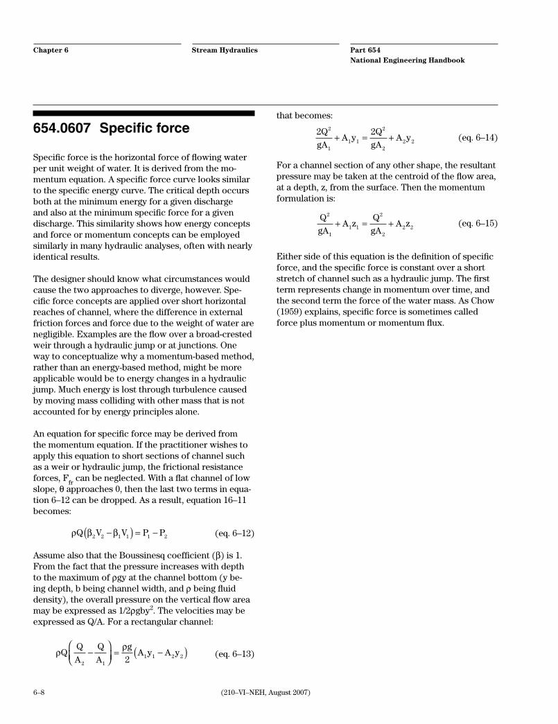
654.0607 Specific force

Specific force is the horizontal force of flowing water per unit weight of water. It is derived from the mo-mentum equation. A specific force curve looks similar to the specific energy curve. The critical depth occurs both at the minimum energy for a given discharge and also at the minimum specific force for a given discharge. This similarity shows how energy concepts and force or momentum concepts can be employed similarly in many hydraulic analyses, often with nearly identical results.

The designer should know what circumstances would cause the two approaches to diverge, however. Spe-cific force concepts are applied over short horizontal reaches of channel, where the difference in external friction forces and force due to the weight of water are negligible. Examples are the flow over a broad-crested weir through a hydraulic jump or at junctions. One way to conceptualize why a momentum-based method, rather than an energy-based method, might be more applicable would be to energy changes in a hydraulic jump. Much energy is lost through turbulence caused by moving mass colliding with other mass that is not accounted for by energy principles alone.

An equation for specific force may be derived from the momentum equation. If the practitioner wishes to apply this equation to short sections of channel such as a weir or hydraulic jump, the frictional resistance forces, F

fr can be neglected. With a flat channel of low

slope, θ approaches 0, then the last two terms in equa-tion 6–12 can be dropped. As a result, equation 16–11 becomes:

ρ β βQ V V P P2 2 1 1 1 2−( ) = − (eq. 6–12)

Assume also that the Boussinesq coefficient (β) is 1. From the fact that the pressure increases with depth to the maximum of ρgy at the channel bottom (y be-ing depth, b being channel width, and ρ being fluid density), the overall pressure on the vertical flow area may be expressed as 1/2ρgby2. The velocities may be expressed as Q/A. For a rectangular channel:

ρρ

QQ

A

Q

A

gA y A y

2 11 1 2 22

−

= −( ) (eq. 6–13)

that becomes:

2 22

11 1

2

22 2

Q

gAA y

Q

gAA y+ = + (eq. 6–14)

For a channel section of any other shape, the resultant pressure may be taken at the centroid of the flow area, at a depth, z, from the surface. Then the momentum formulation is:

Q

gAA z

Q

gAA z

2

11 1

2

22 2+ = + (eq. 6–15)

Either side of this equation is the definition of specific force, and the specific force is constant over a short stretch of channel such as a hydraulic jump. The first term represents change in momentum over time, and the second term the force of the water mass. As Chow (1959) explains, specific force is sometimes called force plus momentum or momentum flux.

6–9(210–VI–NEH, August 2007)



654.0608 Stream power

Stream power is a geomorphology concept that is a measure of the available energy a stream has for mov-ing sediment, rock, or woody material. For a cross sec-tion, the total stream power per unit length of channel may be formulated as:

Ω =

=γγQS

vwdSf

f

(eq. 6–16)

where:γ = unit weight of water (lb/ft3)Q = discharge (ft3/s)S

f = energy slope (ft/ft)

v = velocity (ft/s)w = channel width (ft)d = hydraulic depth (ft)

English units are pounds per second per foot of chan-nel length. A second formulation, unit stream power, is the stream power per unit of bed area:

Ω = τ0 v (eq. 6–17)

where:τ = bed shear stressv = average velocity

A third formulation relates stream power per unit weight of water:

Ω = S vf (eq. 6–18)

where the terms are as previously defined.

654.0609 Hydraulic computations

(a) Uniform flow

Water flowing in an open channel typically gains kinetic energy as it flows from a higher elevation to a lower elevation. It loses energy with friction and obstructions. Uniform flow occurs when the gravita-tional forces that are pushing the flow along the chan-nel are in balance with the frictional forces exerted by the wetted perimeter that are retarding the flow. For uniform flow to exist:

• Mean velocity is constant from section to section.

• Depth of flow is constant from section to section.

• Area of flow is constant from section to section.

Therefore, uniform flow can only truly occur in very long, straight, prismatic channels where the terminal velocity of the flow is achieved. In many cases, the flow only approaches uniform flow.

Since uniform flow occurs when the gravitational forces are exactly offset by the resistance forces, a resistance equation can be used to calculate a veloc-ity. The most commonly used resistance equation is Manning’s equation (eq. 6–19).

Q AR S n

=1 486 2

312

. (eq. 6–19)

given Q VA=

then V R S=1 486 2

312

.

n (eq. 6–20)

where:A = flow area (ft2)R = hydraulic radius (ft)S = channel profile slope (ft/ft)n = roughness coefficient

The 1.486 exponent is replaced by 1.0 if SI units are used. The flow area (A) and the hydraulic radius (R) relate how the flow interacts with the boundary.

6–10 (210–VI–NEH, August 2007)



A rough estimate of the flow capacity or average veloc-ity at a natural cross section may be determined with Manning’s equation. A designer may assume a roughly trapezoidal cross section, estimating bottom width, side slopes, and profile slope from topographic maps. The roughness coefficient is a significant factor, and its determination is described in NEH654.0609(c).

(b) Determining normal depth

Normal depth calculation is one of the most commonly used analyses in stream restoration assessment and design. Several spreadsheets, computer programs, and nomographs are available for use in calculating normal depth. In a natural channel, with a nonuniform cross section, reliability of the normal depth calculation is directly related to the reliability of the input data. Sound engineering judgment is required in the selec-tion of a representative cross section. The cross sec-tion should be located in a uniform reach where flow is essentially parallel to the bank line (no reverse flow or eddies). This typically occurs at a crossing or riffle.

Determination of the average energy slope can be dif-ficult. If the channel cross section and roughness are relatively uniform, surface slope can be used. Thalweg slopes and low-flow water surface slopes may not be representative of the energy slope at design flows. Slope estimates should be made over a significant length of the stream (a meander wavelength or 20 channel widths). Hydraulic roughness is estimated based on field observations and measurements.

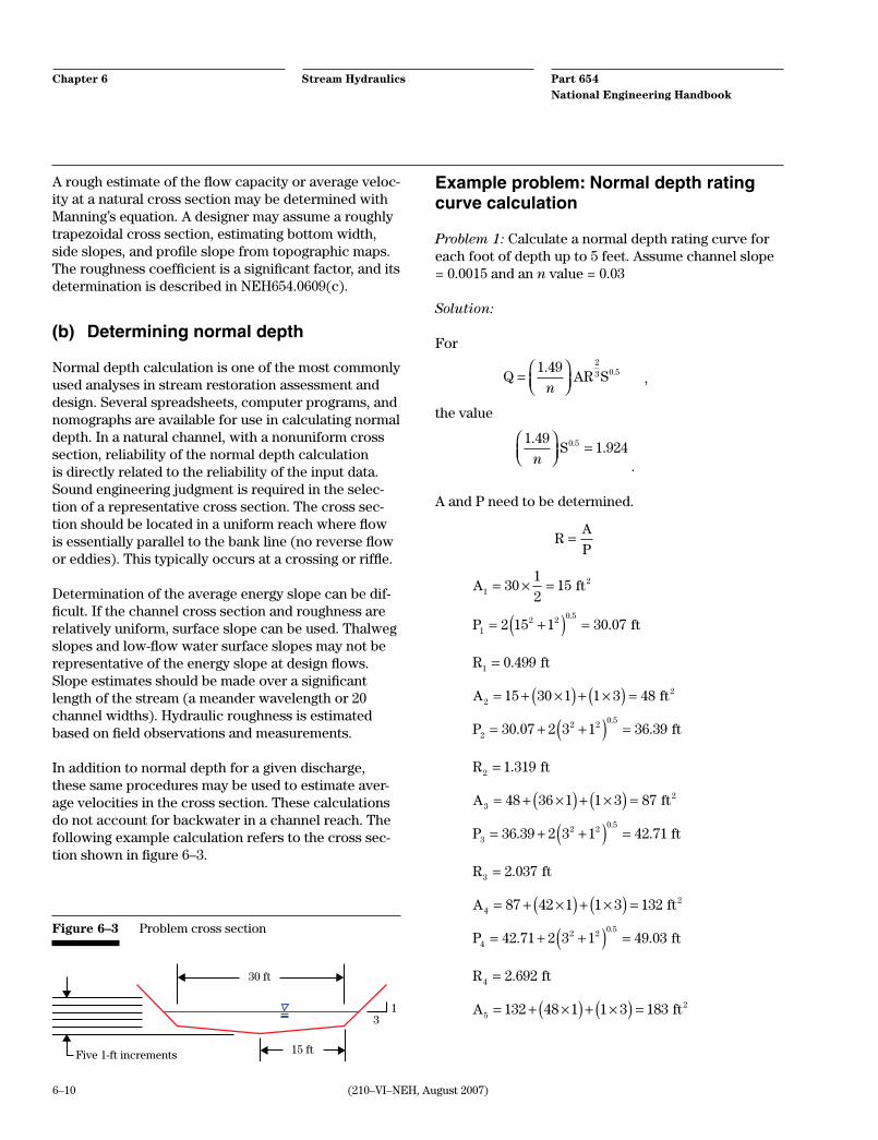
In addition to normal depth for a given discharge, these same procedures may be used to estimate aver-age velocities in the cross section. These calculations do not account for backwater in a channel reach. The following example calculation refers to the cross sec-tion shown in figure 6–3.

Example problem: Normal depth rating curve calculation

Problem 1: Calculate a normal depth rating curve for each foot of depth up to 5 feet. Assume channel slope = 0.0015 and an n value = 0.03

Solution:

For

Q AR S=

1 49 23 0 5. .

n,

the value

1 491 9240 5...

n

=S.

A and P need to be determined.

RA

P=

A1 30

1

215= × = ft2

P1

2 2 0 52 15 1 30 07= +( ) =

.. ft

R1 0 499= . ft

A2 15 30 1 1 3 48= + ×( ) + ×( ) = ft2

P2

2 2 0 530 07 2 3 1 36 39= + +( ) =. .

. ft

R2 1 319= . ft

A3 48 36 1 1 3 87= + ×( ) + ×( ) = ft2

P3

2 2 0 536 39 2 3 1 42 71= + +( ) =. .

. ft

R3 2 037= . ft

A4 87 42 1 1 3 132= + ×( ) + ×( ) = ft2

P4

2 2 0 542 71 2 3 1 49 03= + +( ) =. .

. ft

R4 2 692= . ft

A5 132 48 1 1 3 183= + ×( ) + ×( ) = ft2

Figure 6–3 Problem cross section

13

Five 1-ft increments

30 ft

15 ft

6–11(210–VI–NEH, August 2007)



Figure 6–4 HEC–RAS screen shot for uniform flow computation

P5

2 2 0 549 03 2 3 1 55 36= + +( ) =. .

. ft

R5 3 306= . ft

Solving for Q, then:

Q d1

0 6671 924 15 0 499 18 1 1= × × ( ) = =. . .

. ft /s (at ft)3

Q d2

0 6671 924 48 1 319 111 1 2= × × ( ) = =. . .

. ft /s (at ft)3

Q d3

0 6671 924 87 2 037 269 0 3= × × ( ) = =. . .

. ft /s (at ft)3

Q d4

0 6671 924 132 2 692 491 6 4= × × ( ) = =. . .

. ft /s (at ft)3

Q d5

0 6671 924 183 3 306 781 7 5= × × ( ) = =. . .

. ft /s (at ft)3

Problem 2: Determine the normal depth for a dis-charge of 350 cubic feet per second and the associated average velocity.

Solution: From the rating curve calculated above, the 350 cubic feet per second discharge in this problem will be between Q

3 and Q

4. A straight-line interpolation

gives a depth of 3.4 feet.

For velocity, since Q VA=

V =×( ) + ( ) − ( ) =

350

3 3 4 3 4 8 3 4 43 36

. . .. ft/s

Discussion:The more complicated a section becomes, the more tedious is this hand calculation. Numerous computer programs, such as HEC–RAS (USACE 2001b), can perform normal depth calculations for a cross sec-tion of many coordinate points. A typical image from HEC–RAS is shown as figure 6–4.

6–12 (210–VI–NEH, August 2007)



(c) Determining roughness coefficient (n value)

The roughness coefficient, an empirical factor in Manning’s equation, accounts for frictional resistance of the flow boundary. Estimating this flow resistance is not a simple matter. This parameter is used in com-putation of water surface profiles and estimation of normal depths and velocities.

Boundary friction factors must be chosen carefully, as hydraulic calculations are significantly influenced by the n choice. Factors affecting roughness include ground surface composition, vegetation, channel irregularity, channel alignment, aggradation or scour-ing, obstructions, size and shape of channel, stage and discharge, seasonal change, and sediment transport.

Significant guidance exists in the literature regarding roughness estimation. Chow (1959) discusses four general approaches for roughness determination. The U.S. Geological Survey (USGS) (Arcement and Schneider 1990) published an extensive step-by-step guide for determination of n values. NRCS guidance for channel n value determination is available from Faskin (1963). Finally, when observed flow data and stages are known, manual calculations or a computer program such as HEC–RAS may be used to determine n values.

With the many factors that impact roughness, and each stream combining different factors to different extents, no standard formula is available for use with measured information. As stated in Chow (1959):

...there is no exact method of selecting the n value. At the present stage of knowledge [1959], to select a value of n actually means to estimate the resistance to flow in a given channel, which is really a matter of intan-gibles. To veteran engineers, this means the exercise of sound engineering judgment and experience; for beginners, it can be no more than a guess, and different individuals will obtain different results.

While there has been considerable research on esti-mating roughness coefficients since 1959, flood plain and channel n values are still challenging to determine. In practice, to a large extent the selection of Manning’s n values remains judgement based.

Estimates of channel roughness may be made using photographs or tables provided by Chow (1959), Brat-er and King (1976), Faskin (1963), and Barnes (1967). NEH–5 supplement B, Hydraulics, can also be used to estimate roughness values. As roughness can change dramatically between surfaces within the same cross section, such as between channel and overbanks, a determination of a composite value for the cross sec-tion is necessary (Chow 1959). The choice of a channel compositing method is very important in stream res-toration design where large differences exist in bank and bed roughness. While the following example uses the Lotter method, other methods, such as the equal velocity method and the conveyance method, can also be used.

Example problem: Composite Manning’s n value

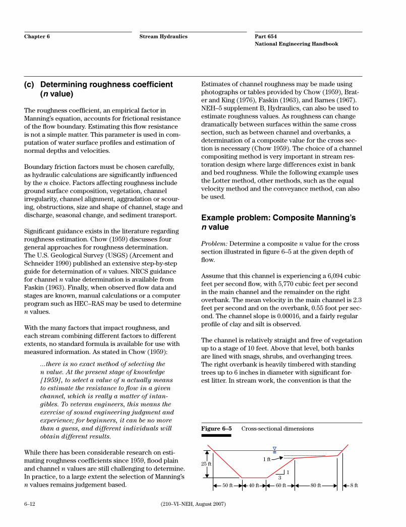
Problem: Determine a composite n value for the cross section illustrated in figure 6–5 at the given depth of flow.

Assume that this channel is experiencing a 6,094 cubic feet per second flow, with 5,770 cubic feet per second in the main channel and the remainder on the right overbank. The mean velocity in the main channel is 2.3 feet per second and on the overbank, 0.55 foot per sec-ond. The channel slope is 0.00016, and a fairly regular profile of clay and silt is observed.

The channel is relatively straight and free of vegetation up to a stage of 10 feet. Above that level, both banks are lined with snags, shrubs, and overhanging trees. The right overbank is heavily timbered with standing trees up to 6 inches in diameter with significant for-est litter. In stream work, the convention is that the

Figure 6–5 Cross-sectional dimensions

13

50 ft

25 ft

40 ft

1 ft

60 ft 80 ft 8 ft

6–13(210–VI–NEH, August 2007)



left bank is on the left when looking downstream. See figures 6–6 and 6–7 where the photos are taken at a lower stage (Barnes 1967).

Solution: To determine the composite Manning’s n value, the inchannel and overbank n values must first be determined.

The solution will first estimate n values using refer-ence materials, then this solution will compare this estimate with the value calculated from Manning’s equation. Roughness estimates can be found in NEH–5, Hydraulics, supplement B by Cowan (1956). Arcement and Schneider (1990) extended this body of work. Both methods estimate a base n value for a straight, uniform, smooth channel in natural materials, then modifying values are added for channel irregular-ity, channel cross-sectional variation, obstructions, and vegetation. After these adjustments are totaled, an adjustment for meandering is also available.

For the channel below 10 feet, the bed material is silty clay. Arcement and Schneider (1990) show base n values for sand and gravel. For firm soil, their n value ranges from 0.025 to 0.032. Cowan (1956) shows a base n of 0.020 for earth channels. Richardson, Si-mons, and Lagasse (2001) shows 0.020 for alluvial silt and 0.025 for stiff clay. A reasonable assumption could be 0.024 for the channel below 10 feet of depth. For the remainder of the channel, above 10 feet of depth to top of bank at 20 feet, the effects of vegetation must be added in. The channel is then divided into three pieces: a lower channel, an upper channel, and a right overbank. Other breakdowns of this cross section are possible.

For the lower channel a base n value of 0.024 is as-sumed. Referring to Cowan (1956) in NEH 5, supple-ment B, a 0.005 can be added for minor irregularity and a 0.005 addition for a shifting cross section. This gives a total n value for the lower channel of 0.034.

Figure 6–6 Looking upstream from left bank Figure 6–7 Looking downstream on right overbank

6–14 (210–VI–NEH, August 2007)



For the upper channel, the area above the lower 10 feet of flow depth and excluding the right overbank, the base n value is 0.024, a minor irregularity addition of 0.005, a 0.005 addition for a shifting cross section, a minor obstruction addition of 0.010, and a medium vegetation addition of 0.020 can be selected. This gives a total n value for the upper channel of 0.064.

For the overbank, a base n (from the overbank soil) is needed. Based on site-specific observations, it was found that the soil is slightly more coarse than that of the main channel, n = 0.027. Again from NEH 5, sup-plement B, Cowan (1956) a minor irregularity addition of 0.005, a shifting cross section addition of 0.005, an appreciable obstruction addition of 0.020, and a high vegetation addition of 0.030 can be selected. This gives a total n value for the overbank of 0.087.

To obtain composite roughness, use the method of Chow (1959), whereby a proportioning is done with wetted perimeter (P) and hydraulic radius (R):

n =

∑

PR

P R

nN N

N

N

53

53

1

(eq. 6–21)

As follows:

P A R nx–s part (ft) (ft2) (ft)

Lower channel 94 650 6.91 0.034

Upper channel 65 1875 28.8 0.064

Right overbank 89 376 4.22 0.087

Total channel 159 2,525 15.88 —

Total x–s 248 2,901 11.70 —

Using equation 6–21 the composite roughness is:

n =( )( )

( )( )+

( )( )+

( )248 11 70

94 6 91

0 034

65 28 8

0 064

89 4

53

53

53

.

.

.

.

.

.222

0 0870 042

53( )

=.

.n

This value can be compared to a value calculated with Manning’s equation as follows.

n =1 486 2

312

.

QAR S

nchan = ( )( ) ( ) =

1 486

57702525 15 88 00016 0 052

23

12

.. . .

Discussion:The difference in Manning’s n initially appears to be cause for concern. However, it does illustrate three important points. First, this process is subjective, and two equally capable practitioners may arrive at differ-ent results. Second, Manning’s equation is for uniform flow. Differences in measured and calculated n values should be attributed to the uncertainty in choosing appropriate values to account for various factors as-sociated with roughness. Manning’s equation by itself can provide an estimate, but it cannot precisely deter-mine roughness when the flow is not uniform. Third, an uncertainty analysis is recommended for hydraulic analysis.

As documented in Barnes (1967), the USGS backwa-ter calculations determined the channel n value to be 0.046 and the right overbank n value to be 0.097. In contrast to this example, Barnes calculated roughness using energy slope, rather than water surface slope and also included expansion and contraction losses.

Example problem: Manning’s n value for a sand-bed channel

Problem: Determine the n value for a wide, sand chan-nel with the following cross section (fig. 6–8). Assume a discharge of 4,100 cubic feet per second, a thalweg depth of 5 feet, 3:1 side slopes and a fairly straight, regular reach. Assume a slope of 0.0013 and a sandy bottom with a D

50 of 0.3 millimeter.

Figure 6–8 Sand channel cross section

125 ft

35 ft2 ft2 ft

6–15(210–VI–NEH, August 2007)



Solution: Roughness in sand channels is highly de-pendent on the channel bedforms, and bedforms are a function of stream power and the sand gradation. Ar-cement and Schneider (1990) show suggested n values for various D

50 values with the footnote that they apply

only for upper regime flows where grain roughness is predominant. For a D

50 of 0.3 millimeter, this reference

suggests a 0.017 n value. However, it is important to assess the regime of the flow. A figure from Simons and Richardson (1966) (also in Richardson, Simons, and Lagasse 2001 and Arcement and Schneider 1990) is shown as figure 6–9. Given stream power and me-dian fall diameter, the flow regime may be estimated, as well as the expected bedform and roughness range.

Stream power may be calculated from where gamma is unit weight of water, Q is discharge, and S

f is the

Figure 6–9 Plot of flow regimes resulting from stream power vs. median fall diameter of sediment

3

2

1

0.8

Upper regime

Upper flow regimePlane bed (0.010≤n≤0.013)Antidunes Standing waves (0.010≤n ≤0.013) Breaking waves (0.012≤n≤0.020)Chute and pools (0.018≤n≤0.035)

Lower flow regimeRipples (0.018≤n≤0.028)Dunes (0.020≤n≤0.040)

Lower regime

Transition

Str

eam

po

wer

, 62

RS

wV

(ft

-lb

/s/f

t2 )

0.6

0.4

0.20 0.2 0.4 0.6

Median grain size (mm)

0.8 1 1.2

energy slope. Assuming the energy slope is nearly the same as the bed slope, then:

Ω = ( )( )( )=

62 4 4100 0 0013

333

. . lb/ft ft /s

lb/s

3 3

(per ft of channel length)

For figure 6–9, stream power per cross-sectional area is needed. The flow area for the given cross section is 554 ft2, so the stream power is 0.60 pounds per second per square foot (per foot of channel length). Read-ing figure 6–9, with a D

50 of 0.3 millimeter, the flow is

in the upper regime, but close to the transition. This would support an n value of 0.017, particularly if bed-forms are present.

6–16 (210–VI–NEH, August 2007)



Figure 6–10 (Arcement and Schneider 1990) indicates the general bedforms for increasing stream power.

The anticipated bedform is a plane bed, and figure 6–9 suggests an n value between 0.010 and 0.013 for plane beds. The presence of breaking waves over antidunes would raise the roughness estimate to between 0.012 to 0.02. Finally, an estimate may be calculated with the Strickler formula (Chang 1988; Chow 1959) that relates n value to grain roughness. So, for a plane bed it should give a good estimate:

n = ( )0 0389 50

16. D with D

50 in feet (eq. 6–22)

or

n = ( )0 0474 50

16. D with D

50 in meters (eq. 6–23)

Since the D50

is 0.3 millimeter, the calculated n value is 0.012, which agrees with figure 6–9 results for plane beds. Arcement and Schneider (1990) show n = 0.012 for a D

50 of 0.2 millimeter, and this calculation is close

to the transition range. Considering all of the above, information supports a roughness selection between 0.013 to 0.017. If field observations support the plane

bed assumption, a value from the low end of this range should be selected. If antidunes are present, a value from the high end of this range would be reasonable.

Example problem: Manning’s n value for a gravel-bed channel

Problem: Determine the n value for a wide, gravel-bed channel with a D

50 of 110 millimeters. Assume a fairly

straight, regular reach. Assume minimal vegetation and bedform influence.

Solution: Since the grain roughness is predominant, the Strickler formula can be used.

n = ( )0 0474 50

16. D for D

50 in meters

This results in an estimated n value of 0.033. It should be noted that this estimate does not take into account many of the factors which influence roughness in natural channels. As a result, a estimate made with Strickler’s equation is often only used as an initial, rough estimate or as a lower bound.

Figure 6–10 General bedforms for increasing stream power

Plane bed

Watersurface

Resistance to flow(Manning’s roughnesscoefficient)

Transition

Stream power

Bedform

Upper regimeLower regime

Bed

Ripples Dunes Transition Plane bed Standing wavesand antidunes

6–17(210–VI–NEH, August 2007)



(d) Friction factor

As with Manning’s n value and the Chézy C, the fric-tion factor, f, is a roughness coefficient in a velocity equation, namely, the Darcy-Weisbach equation. Origi-nally developed for pipe flow, the equation adapted for flow in open channels is:

VgRS

f=

80 5.

with f being dimensionless. (eq. 6–24)

Alternatively, fgRS

V=

82 (eq. 6–25)

In 1963, the ASCE Task Committee on Friction Factors in Open Channels recommended the preferential use of the Darcy-Weisbach friction factor over Manning’s n (Simons and Sentürk 1992). While Manning’s equation remains the most used equation in practice, a compari-son between the two is an illustrative exercise. The equation, applicable for steady uniform flow, is a bal-ance of downstream gravitational force and upstream boundary resistance forces. The relationship between Manning’s n and Chézy C is (Hey 1979, English units):

80 5

16

0 5 0 5f

d

g

C

g

= =.

. .n (eq. 6–26)

where:d = hydraulic depth

To apply the velocity equation, the friction factor must be determined. As has often been discussed by researchers (Raudkivi 1990; Thorne, Hey, and New-son 2001), the vertical velocity profile can often be assumed to be logarithmic with distance from the bed. For sand and gravel channels, where the relative roughness (flow depth/bed-material size) exceeds 10, this relationship holds.

For use in gravel-bed streams, with width-to-depth ratios greater than about 15, Hey (1979) derived the following (see also Thorne, Hey, and Newson 2001):

1

2 033 5 84f

aR

D= . log

. (SI units) (eq. 6–27)

or

8

5 753 5

0 5

84f

aR

D

=.

. log.

(English units) (eq. 6–28)

where:R = hydraulic radiusD

84 = bed-material size for which 84 percent is small-

er

The dimensionless a is given by (Thorne, Hey, and Newson 2001):

aR

max

=

−

11 1

0 314

.

.

d (eq. 6–29)

where:d

max = maximum flow depth

The coefficient a varies from 11.1 to 13.46 and is a function of channel cross-sectional shape. For chan-nels in which the width-to-depth ratio exceeds 2, the maximum flow depth is valid in the above equation. Otherwise, the value in the denominator should be the distance perpendicular from the bed surface to the point of maximum velocity. This formula for determin-ing f may be used in gravel-bed riffle-pool streams in the riffle section, where flow is often assumed to be uniform. In general, the D

84 is calculated based on a

sample taken at the riffle section.

The Limerinos equation can also be used to determine the friction factor.

n =

( )+

0 0926

1 16 2 0

16

84

.

. . log

R

rD

(eq. 6–30)

where:R = hydraulic radius, in ftD

84 = particle diameter, in ft, that equals or exceeds

that of 84 percent of the particles

This equation was developed from samples taken from 11 large United States rivers with bed materials rang-ing from small gravel to medium size boulders. This equation has been shown to work well on sand-bed streams with plane beds.

(e) Accounting for velocity distributions in water surface profiles

Actual velocities in a cross section are distributed from highest, generally in the center at a depth that is some small proportion beneath the surface, to much

6–18 (210–VI–NEH, August 2007)



lower values in overbanks and at flow boundaries (fig. 6–11). A velocity meter measures velocities related to the vertical flow area close to the instrument.

This elementary phenomenon is responsible for the fact that an average cross-sectional velocity cannot provide a precise measure of the kinetic energy of the flow; the alpha and beta coefficients therefore are needed as modifiers.

When the flow velocity in a cross section is not uni-formly distributed, the kinetic energy of the flow, or velocity head, is generally greater than V2/2g, where V is the average velocity. The true velocity head may be approximated by multiplying the velocity head by alpha (α), the energy coefficient. Chow (1959) stated that experiments generally place alpha between 1.03 and 1.36 for fairly straight prismatic channels. The nonuniformity of velocity distribution also influences momentum calculations (as momentum is a function of velocity).

Beta (β) is the momentum coefficient that Chow indicates varies from 1.01 to 1.12 for fairly straight prismatic channels. Beta, also called the Boussinesq coefficient, is also described in Chow (1959). Both coefficients may be calculated by dividing the flow area into subareas of generally uniform velocity distri-bution. α ≈ ∑ v A

V Ai3

i

3total

(eq. 6–31)

β ≈ ∑ v A

V Ai2

i

2total

(eq. 6–32)

However, for natural channels, the calculation is better made using conveyance. HEC–RAS uses the following formulas:

α ≈

∑ K

A

K

A

i3

i2

total3

total2

(eq. 6–33)

β ≈

∑ K

A

K

A

i2

i

total2

total

(eq. 6–34)

Every cross section is only a two-dimensional slice of a three-dimensional reality. Cross sections change along the stream profile, inevitably setting up trans-verse velocity vectors, and the flow is induced into a roughly spiral motion. This flow behavior leads to point bars, pools and riffles, meandering patterns, and flood plains. Further information on the velocity and shear in the design of streambank protection in bends is given in NEH654.14, Stabilization Techniques.

(f) Determining the water surface in curved channels

Water surface profiles as computed by HEC–RAS assume a level water surface in each cross section. This is not the case in a curved channel. However, the water surface calculated by HEC–RAS is valid along the centerline of the flow. Generally, HEC–RAS can account for the friction and eddy losses caused by a bend so that the water surface computed upstream would be correct. However, the super-elevated water surface in the bend itself must be calculated separate-ly. The following formula is often used for estimating super-elevation in a water surface.

∆Z

bV

grc

=2

(eq. 6–35)

where:V = average channel velocity (ft/s)b = channel top width (ft)g = gravitational acceleration (32.2 ft/s2)r

c = radius of curvature of the channel (ft)

∆Z = super-elevation in ft from bank to bank, so the amount added to or subtracted from the cen-terline elevation would be half that. A factor of safety of 1.15 is generally applied.

Figure 6–11 Flow velocities for a typical cross section

6–19(210–VI–NEH, August 2007)



In supercritical flow, curved channels are much more complicated due to wave patterns that propagate back and forth across the channel and downstream. With the disturbances reflecting from one side to the other, higher water surfaces can occur both on the inside and outside banks of a bend. Although a methodology for determining the super-elevation is developed by Chow (1959) for a regular curved channel with a constant width, it also approximates that for a natural channel.

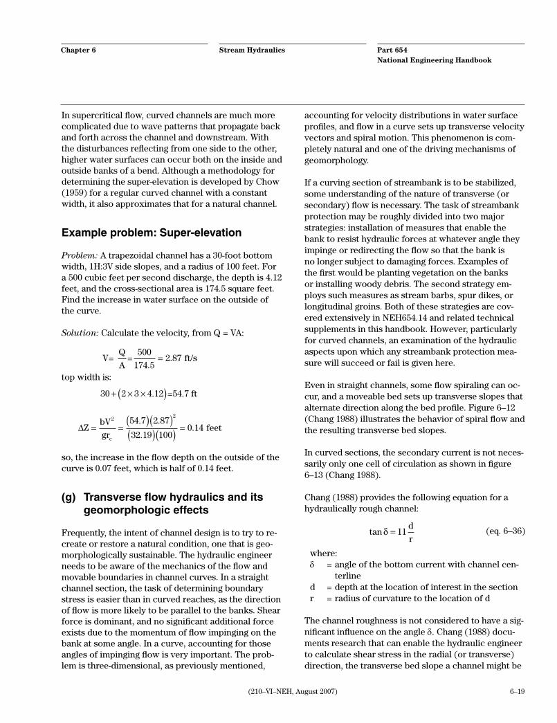
Example problem: Super-elevation

Problem: A trapezoidal channel has a 30-foot bottom width, 1H:3V side slopes, and a radius of 100 feet. For a 500 cubic feet per second discharge, the depth is 4.12 feet, and the cross-sectional area is 174.5 square feet. Find the increase in water surface on the outside of the curve.

Solution: Calculate the velocity, from Q = VA:

V= Q

A=

500

174.5 ft/s= 2 87.

top width is:

30 2 3 4 12+ × ×( ). =54.7 ft

∆Z

bV

grc

= =( )( )( )( ) =

2 254 7 2 87

32 19 1000 14

. .

.. feet

so, the increase in the flow depth on the outside of the curve is 0.07 feet, which is half of 0.14 feet.

(g) Transverse flow hydraulics and its geomorphologic effects

Frequently, the intent of channel design is to try to re-create or restore a natural condition, one that is geo-morphologically sustainable. The hydraulic engineer needs to be aware of the mechanics of the flow and movable boundaries in channel curves. In a straight channel section, the task of determining boundary stress is easier than in curved reaches, as the direction of flow is more likely to be parallel to the banks. Shear force is dominant, and no significant additional force exists due to the momentum of flow impinging on the bank at some angle. In a curve, accounting for those angles of impinging flow is very important. The prob-lem is three-dimensional, as previously mentioned,

accounting for velocity distributions in water surface profiles, and flow in a curve sets up transverse velocity vectors and spiral motion. This phenomenon is com-pletely natural and one of the driving mechanisms of geomorphology.

If a curving section of streambank is to be stabilized, some understanding of the nature of transverse (or secondary) flow is necessary. The task of streambank protection may be roughly divided into two major strategies: installation of measures that enable the bank to resist hydraulic forces at whatever angle they impinge or redirecting the flow so that the bank is no longer subject to damaging forces. Examples of the first would be planting vegetation on the banks or installing woody debris. The second strategy em-ploys such measures as stream barbs, spur dikes, or longitudinal groins. Both of these strategies are cov-ered extensively in NEH654.14 and related technical supplements in this handbook. However, particularly for curved channels, an examination of the hydraulic aspects upon which any streambank protection mea-sure will succeed or fail is given here.

Even in straight channels, some flow spiraling can oc-cur, and a moveable bed sets up transverse slopes that alternate direction along the bed profile. Figure 6–12 (Chang 1988) illustrates the behavior of spiral flow and the resulting transverse bed slopes.

In curved sections, the secondary current is not neces-sarily only one cell of circulation as shown in figure 6–13 (Chang 1988).

Chang (1988) provides the following equation for a hydraulically rough channel:

tan δ = 11d

r (eq. 6–36)

where:δ = angle of the bottom current with channel cen-

terlined = depth at the location of interest in the sectionr = radius of curvature to the location of d

The channel roughness is not considered to have a sig-nificant influence on the angle δ. Chang (1988) docu-ments research that can enable the hydraulic engineer to calculate shear stress in the radial (or transverse) direction, the transverse bed slope a channel might be

6–20 (210–VI–NEH, August 2007)



Figure 6–12 Spiral flow characteristics for a typical reach

Surface current

Innerbank

Outerbank

Bottom current

δ

Figure 6–13 Flow characteristics for a typical reach

δ

β

d

Profile slopeBottomcurrent

CL

r

6–21(210–VI–NEH, August 2007)



expected to acquire, and the sediment sorting expect-ed along that transverse slope.

Chang (1988) provides the following two equations to calculate shear stress in the radial direction (both toward the inside of the curve, due to bottom current, and toward the outside due to surface current):

τ ρκ κ0r

2U

r

g g= −

−

dC C

2 2

2 3

(eq. 6–37)

τ ρ0r2d

rU=

++

1

22

m

m m (eq. 6–38)

m

f= κ

8 (eq. 6–39)

where:ρ = density of waterg = acceleration due to gravityκ = the dimensionless von Kármán constant

(κ ≈ 0.40)U = avg. cross-sectional velocityC = Chézy resistance factor, defined belowd = depth at the location of interestr = radius of curvature to that locationf = friction factor as defined below

The Chézy resistance factor is similar to Manning’s n value in that it is an empirically derived coefficient serving as an index of boundary roughness. The fol-lowing Ganguillet and Kutter formula (1869), as pro-vided in Chow (1988), is a method of calculating Chézy C, given Kutter’s n:

C nn

=+ +

+ +

41 650 00281 1 811

1 41 650 00281

.. .

..

S

S R

(eq. 6–40)

where:S = profile bed slopeR = hydraulic radiusn = Kutter’s roughness

Chézy’s C is related to Manning’s n by the following equation in English units:

C

R

=

1 48616.

n (eq. 6–41)

R = hydraulic radius (ft)

The Darcy-Weisbach friction factor, f, is described by Chow (1959) and for uniform or near uniform flow may be calculated using:

f =8gRS

V2 (eq. 6–42)

Both Chow (1959) and Chang (1988) describe the relationship of f to boundary Reynolds number. Chang provides three formulas, dependent on hydraulic smoothness, for channels in which form roughness is not a factor as follows.

f

R k

Rbed s= +( ) <

−0 103 2

40 5

5. log log .

.R forbed

(eq. 6–43)(hydraulically smooth)

where:R = hydraulic radiusR

bed= boundary Reynolds number

ks = equivalent roughness or grain roughness,

calculated from the following, one of several similar equations, Chang (1988):

k Ds = 3 90 (eq. 6–44)

For the transition from hydraulically smooth to rough:

f AR k

R

R

kibed s

i

i s

=

+

≤

=

−

∑ log log

.

42

2

0

65

for

0.5 logRbedd s

4R

k≤ 2 0.

(eq. 6–45)

where the coefficients A0 through A

6 are 1.3376,

-4.3218, 19.454, -26.48, 16.509, -4.9407, and 0.57864, respectively.

For the hydraulically rough regime:

f

k

k= +

>−

1 74 22

2 0

5

. log .

.R

for logR

4Rs

bed s

(eq. 6–46)

6–22 (210–VI–NEH, August 2007)



For gravel-bed rivers, Chang (1988) provides the fol-lowing equation:

fD

= +

−

0 248 2 36

5

. . log

.d

50

(eq. 6–47)

where:d = max depth of flow with units same as D

50

In figure 6–13, δ is the angle between the velocity vec-tor of the bottom current and the centerline. Also of interest is the resultant angle of shear stress between the two components of shear, and longitudinal and radial. Chang (1988) gives that angle, δ , as:

tan ′ = −

δ

κ κ2

1d

C2r

g (eq. 6–48)

where all variables have been previously defined.

Longitudinal shear stress at any point in the cross sec-tion is calculated with the following equation:

τ γ0s ccS

r

r= d (eq. 6–49)

where the c subscript refers to the channel centerline.

The transverse bed slope (β) can be computed using:

β δ ϕ= ( )arctan tan tan (eq. 6–50)

where:δ = the angle shown in the above sketchϕ = the sediment angle of repose

This equation is valid when β is small compared to ϕ. This relationship is less accurate for channels with significant quantities of suspended sediment. Since ϕ is generally >30º, then β should be less than 10º. If ϕ >30º, then β becomes less valid as δ increases toward 20º or in tight curves.

Finally, Chang (1988) provides a formula for determin-ing sediment sorting on the transverse slope:

Dd

=−( )

3

2

ρρ ρ ϕ

S r

r tanc c

s

(eq. 6–51)

where:D = median grain sized = depth at that locationS

c = longitudinal profile slope along the centerline

rc = radius of curvature to centerline

r = radius of curvature to location of dρ = densities of sediment and water

Example problem: Design radius

Problem: A roughly trapezoidal curved channel is being designed with a moveable boundary in dynamic equilibrium to carry a flow of 700 cubic feet per sec-ond. The channel profile slope is 0.0013, channel bot-tom width is 30 feet, with a transverse bed slope, β, of 10 percent, and 3H:1V side slopes. The bed material is rounded gravel, with a D

50 of 0.30 inches, and n value

of 0.035. Considering uniform flow and a maximum depth of 6 feet, calculate the design radius of curva-ture to the centerline, longitudinal and radial stress vectors at the centerline, and the resultant stress angle in the curve.

Solution:Part 1—Design radius of curvature to the centerline

The angle of repose ϕ for 0.3-inch, rounded gravel is about 31 degrees. Assuming a constant transverse bed angle of 10 percent, tan β = 0.10, and the resulting angle of the bottom current would be:

tan tan β δ ϕ= tan (eq. 6–52)

or

δβϕ

=

arctantan

tan (eq. 6–53)

so, δ = 9.4 degrees

Consider the channel centerline to be horizontally located at the centroid of the flow cross section, as shown in figure 6–14.

Figure 6–14 Channel centerline at centroid of flow

3 ft6 ft

30 ft

X

D

r

6–23(210–VI–NEH, August 2007)



To find X, the flow area left of the centroid must be equated to that on the right:

18 6

23

30 3

2

30 3 0 1

2

3 309 3

2

30 3 0 1

×+ +

×−

−( ) −( )

= −( ) +×

+−( ) −( )

XX X

XX X

.

.

22

Simplifying:

54 3 45 90 3 13 5 30 3 0 1+ + = − + + −( ) −( )X X XX . .

12 94 5X 0.1X2− = .

by trial and error, X = 8.5 feet.

The depth at the centerline is

6 8 5 0 10 5 15− ( )( ) =. . . ft

given:

tan δ = 11d

r, solving for radius of curvature, r = 342 ft

Part 2—Longitudinal and radial stress vectors

The longitudinal shear stress at the centerline is calcu-lated with equation 6–49.

τ γ0s cc 2S

r

r lb/ft= = × × =d 62 4 5 15 0 0013 0 418. . . .

The total flow area is 202.5 square feet, wetted pe-rimeter = 58.6 feet, so R = 3.46 feet. From Q = VA, the average velocity is 700/202.5 = 3.46 feet per second. The friction factor is:

f = =× × ×

( )=

8 80 097

gRS

V

32.19 3.46 0.0013

3.462 2

.

The radial shear is calculated with equations 6–38 and 6–39.

τ ρ0r2d

rU=

++

1

22

m

m m

m

f= = =κ

8 80 4

0 0973 36.

..

τ0r

2

1.948 lb-s /ft ft

342 ft(3.46 = × × × ×0 242

5 153

..slugs

ft slugfft/s

lb/ft

2

2

)

.= 0 085

Part 3—Resultant stress angle in the curve

The direction of the resultant stress vector between the longitudinal and radial components is calculated using equations 6–48 and 6–40.

tan ′ = −

δ

κ κ2

1d

C2r

g

where:

C S

S R

=+ +

+ +

41 650 00281 1 811

1 41 650 00281

.. .

..

nn

C =+ +

+ +

41 650 002810 0013

1 8110 035

1 41 650 002810 0013

...

.

.

...

=0 035

52 4.

.

3.46

tan.

..′ =

×

( ) ×−

×

=

′ = °

δ

δ

2 5 151

52 40 137

8

0.4 342

32.19

0.42

Hey (1979) addresses point bar development with a sketch similar to figure 6–15, showing how secondary currents, along with bed-load supply, impact the loca-tion of aggradation and degradation in a meander.

During bankfull flows, the strongest velocity vectors follow the course of the arrows starting at A in figure 6–15, cutting across the toe of point bars with the high-est bed-load supply. At B, downstream of the bar apex, the shear stress and transport capacity drop, and ag-gradation occurs. Opposite the point bar at C, low bed load accompanies the incoming flow, and as surface

Figure 6–15 Point bar development

D

C

B

EA

6–24 (210–VI–NEH, August 2007)



currents angle into the bank and undercurrents move away from the bank, a zone of downwelling results at point D. The low bed load gives the stream a scouring tendency. Toward the inflection point of the meander, flow with a low bed-load supply enters a contracted reach at E that is steeper and shallower, and regains its scouring capacity. Riffles form and, as the highest velocity vectors cut from one point bar toe to the toe of the next downstream bar, riffles are often skewed to the banks.

(h) Change in channel capacity

Natural channels will often incise in response to hu-man impacts, such as watershed development, channel straightening, removal of vegetation, or overgrazing. The incision is a lowering of the channel bed, that in effect increases the channel size and capacity. Often, the overbank dries out due to a falling water table. This lowered water table can cause wetlands to shrink

Figure 6–16 Seasonal hydrograph

400

350

300

250

200

150

100

Flo

w (

ft3 /s

)

1-May 8-May 15-May 22-May 29-May 5-Jun 12-Jun 19-Jun 26-Jun

and adjacent productive lands to depend on irriga-tion. For projects in which overbank soil moisture is a concern, the duration of flow is often more important than the peak discharge. Inchannel flow can have a significant effect on overbank soil moisture if it is near bankfull for a sufficient duration.

Example problem: Change in overbank duration

Problem: A channel has, in the span of 10 years, in-cised by several feet and increased the bankfull flow area from 84 square feet to 107 square feet. The chan-nel slope has increased from 0.0020 to 0.0025. The wet-ted perimeter increased from 29.4 feet to 42 feet. The vegetation has suffered to the extent that composite n value has decreased from 0.045 to 0.038. Approximate the change in duration of overbank flooding, given the season-long hydrograph in figure 6–16.

6–25(210–VI–NEH, August 2007)



Solution: Using a uniform flow assumption and Man-ning’s equation, the original channel capacity was:

Q AR S=

= ( )

( )

=

1 486

1 486

0 04584

84

29 40 002

250

23

12

23 1

2

.

.

. ..

n

fft s3 /

With the changed hydraulic parameters:

Q

1.486107

107

420.0025

ft /s

23

3

= ( )

( )

=

0 038

390

12

.

Looking at the hydrograph, then, the new channel condition fully contains the hydrograph, since the peak is less than 390 cubic feet per second: no days of overbank flooding occur. The previous channel capac-ity was 250 cubic feet per second, and overbank flow would have occurred four separate times for a total of about 16 days.

654.0610 Water surface profile calculations

The calculation of water surface profiles and associat-ed hydraulic parameters is a common task of hydrau-lic engineers. In natural, gradually varied channels, velocity and depth change from cross section to cross section. However, the energy and mass are conserved. The energy and continuity equations can be used to step from a water surface elevation at one cross sec-tion to a water surface at another cross section that is a given distance upstream (subcritical) or downstream (supercritical). Programs, such as HEC–RAS, use the one dimensional energy equation, with energy losses due to friction evaluated with Manning’s equation, to compute water surface profiles. Equation 6–9 be-comes:

V

2g

V

2g

2

2

2

1

+ + =

+ + +Y Z Y Z he2 2 1 1 (eq. 6–54)

This one dimensional energy equation can be restated as:

WS WSg

V V he2 1 1 12

2 221

2= + −( ) +α α (eq. 6–55)

The water surface profile determination is accom-plished with an iterative computational procedure called the standard step method. This is graphically illustrated in figure 6–17.

Figure 6–17 Standard step method

Datum

Z

Y2

(V2/2g)2

Z

Y1

he

(V2/2g)1

Channel bottom

Water surface

Energy grade line

6–26 (210–VI–NEH, August 2007)



The energy loss includes friction losses (usually evalu-ated with Manning’s equation) and losses associated with changes in cross-sectional areas and velocities. This is represented in equation 6–56:

h LS CV

g

V

ge f= + −α α2

212

2 2 (eq. 6–56)

Friction loss is evaluated as the product of the friction slope and the discharge weighted reach length. This is shown in equation 6–57:

LL Q L Q L Q

Q Q Qlob lob ch ch rob rob

lob ch rob

=+ +

+ + (eq. 6–57)

Example problem: Backwater from a log drop

Problem: Determine the maximum crest level of a log weir set all the way across the channel that would cause no backwater, and the crest level required to cause 1 foot of backwater just upstream of the weir (fig. 6–18). Assume a discharge of 491.5 cubic feet per second, depth of 4 feet, and uniform flow conditions without the weir.

Solution: To create no backwater, the log weir would have to pass the same discharge at the same water surface. The evaluation should be between the log

crest (section 2) and a point (section 1) not very far upstream (fig. 6–19).

This can be evaluated using the energy approach with Bernoulli’s equation. An assumption can be made that there is very little friction loss between the two points. The difference in the channel bottom elevation is also negligible over this short distance. So,

z yV

z yV

hL1 112

2 222

2 2+ + = + + +α α1 2g g

where:h

L = head loss (assumed negligible) becomes:

yV

gy

V

gD1

12

222

2 2+ = + +

where: D = height of the log weir

If the flow is high enough, the log weir will be drowned out by the normal depth tail water and would not cause backwater. At lower discharges, the flow over the log will pass through critical depth (as shown in fig. 6–19).

At critical depth, the velocity head is equal to half the hydraulic depth:

Vcr2

2g

d

2

A

2T= =

Figure 6–19 Profile for crest of log weir problem

D

21

H1

3 (typ)

Crest of log weir

1 ft

15 ft 15 ft

Figure 6–18 Problem determinations for determination of log weir

6–27(210–VI–NEH, August 2007)



Substituting back into Bernoulli’s equation, since V2 is

Vcr

,

yV

y112

2+ = + +

g

A

2TDcr

To determine whether the log causes backwater, com-pare the y

1 calculated to the flow depth without the log

(4 ft). That is:

yV

cr

A

2TD

g+ + − 1

2

2 less than 4

where:V

1 = velocity upstream of the weir

Using the critical depth formula (where d is hydraulic depth and T is top width) along with the continuity equation, Q = VA, the following can be derived:

Vcr2

2g

d

2

A

2Tcr= =

AQ

crcr

=V

and Vcr2 = =

A 2g

2T

A g

Tcr cr

AQ

cr

2

cr

22

=V

so AQ T

A gcr2

2

cr

= and AQ T

gcr

2

3=

To find the maximum log crest before backwater is created, a log crest must be chosen and checked with a trial and error approach. For this example, suppose D = 1. Choose a depth and calculate the flow area by the dimensions of the cross section. Then compare with the A

cr. When the two flow areas are the same,

this is the critical depth for that Q (given as 491.5 ft3/s).

Trial # ycr T A Acr

1 1.0 36.0 33.0 64.65

2 2.0 42.0 72.0 68.06

3 1.9 41.4 67.8 67.70

However, the velocity head must still be calculated to assure that there is no backwater. Note that the veloc-ity head is negligible as long as the velocity is not too large. For example, a velocity of 5 feet per second results in a velocity head of 0.39 feet.

yV

cr1A

2TD

g+ + −

2

2 less than 4

If this velocity head term is neglected, then giveny

cr = 1.9, T = 41.4, A = 67.8, the above formula solves

as:

1 9 3 72. .+×

+ =67.8

2 41.41 ft

Since this solution is less than the clear channel depth of 4, it may be possible to raise the weir.

(a) Steady versus unsteady flow

Many hydraulic parameters of interest in typical de-signs and assessment can be calculated by assuming a normal depth. Normal depth calculations are often based on a solution to Manning’s equation. This ap-proach is relatively simple, but only applicable in uniform flow conditions where the gravitational forces are exactly offset by the resistance forces. Manning’s equation is an infinite slope model that assumes mean depth, velocity, and area are the same from cross section to cross section. It can only occur in long, straight, prismatic channels where the terminal veloc-ity of the flow is achieved. This assumption cannot account for backwater conditions nor variable chan-nel shape, roughness, and slope. Natural channels approach, but rarely achieve uniform, normal depth. Designs and assessments that depend on calculations based on normal depth must consider the affects of possible errors.

Even though flows in a stream are readily observable at any time, they are unsteady at every spatial and temporal scale. Typically, unsteady modeling results in variations in flow rate, velocity, and depth in space and time throughout the modeled reach. In most unsteady flow models, the discharges can vary within a model, and the boundary conditions are in terms of flow and stage with time. Unsteady flow calculations are often used to analyze a dam breach, inchannel storage, vari-able boundary conditions, rapidly rising hydrographs on flat slopes, irrigation withdrawals, tributary flow interaction, and locations where duration of flooding is an issue.

Unsteady flow models can be contrasted to steady flow models with no time component in the calcula-tions. Steady flow models are typically much simpler to calibrate and execute than unsteady flow models. For most steady flow models, the depth and velocity

6–28 (210–VI–NEH, August 2007)



may change from section to section, but only one flow is allowed per section per model run. Since the flow is constant with respect to time, only one discharge is calculated for each section in a given steady flow model run. In addition, boundary conditions are held constant. These assumptions are often suitable for many analyses where the reach is short or the primary interest is an assessment of the peak hydraulic param-eters for a given discharge.

In alluvial channels, the interaction of sediment with the flow can also have a profound affect since the amount and type of sediment load affects the energy balance of the flow. Equations of sediment motion (sediment continuity and sediment transport) are cov-ered in NEH654.13.

(b) Backwater computational models

Computer programs are used to calculate water sur-face profiles, lateral velocity distributions, flow re-gimes, and scour potential. For projects that are likely to involve revisions to Federal Emergency Manage-ment Agency’s (FEMA) Flood Insurance Rate Maps, selection of the hydraulic model should be coordinat-ed carefully with FEMA. Following are some standard hydraulic models.

HEC–RASHEC–RAS (USACE 2001b) is the recommended com-puter program for performing hydraulic calculations for steady and unsteady, gradually varied (over dis-tance), one-dimensional, open channel flow. HEC–RAS includes a culvert module that is consistent with HDS–5 and HY–8. The bridge hydraulics algorithms now include the WSPRO models. HEC–RAS applies conser-vation of momentum, as well as energy and mass, in its hydraulic analysis. HEC–RAS includes all the features inherent to HEC–2 and WSPRO, plus several friction slope methods, mixed flow regime support, automatic n value calibration, ice cover, quasi 2–D velocity distri-bution, and super-elevation around bends.

HEC–2HEC–2 (USACE 1990b) performs hydraulic calcula-tions for steady, gradually varied (over distance), one-dimensional, open channel flow. One of HEC–2’s technical limitations is that the normal bridge routines and standard-step backwater computations use energy conservation only. Conservation of momentum is used

only in the special bridge routines when bridge piers are involved.

WSPROThe WSPRO computer program was developed by the USGS and is comparable to HEC–2, except for the fact that WSPRO had special subroutines for analysis of water surface profiles at bridge locations. All of these WSPRO subroutines have been incorporated into HEC–RAS. The current version of WSPRO is no longer being supported by USGS.

HY–22HY–22 is a small tool kit of relatively simple computer programs for performing the hydraulic analyses de-scribed in the Urban Drainage Design Manual, Hy-draulic Engineering Circular No. 22, U.S. Department of Transportation Federal Highway Administration (FHWA) (1996). HY–22 includes pavement drainage, open channel hydraulics, critical depth computation, computation of storage volume, and simple reservoir routing.

6–29(210–VI–NEH, August 2007)



654.0611 Weir flow

Flow over a broad-crested weir is an application that can be analyzed with momentum principles. The mo-mentum principle has certain advantages in applica-tion to problems involving high internal energy chang-es (Chow 1959). The pressure force due to the weight of water and the obstruction of the weir is important. The gravitational force vector in the direction of flow may be neglected for a mild channel slope and small distance between the uncontracted upstream section and the cross section at the weir. The friction forces on the wetted boundary in the short distance between the two sections may be neglected, as well.

Weir flow is calculated using:

Q CLH=32 (eq. 6–58)

where:L = weir length (ft)C = weir discharge coefficient (usually from 3.05 to

2.67)H = approach head (ft)

The actual value of C depends on factors such as the roundedness of the upstream corner of the weir and the width and slope of the weir crest. Brater and King (1976) give C = 3.087 as a maximum value for broad-crested weirs with a vertical upstream face under any conditions, given that the upstream corner is so rounded as to prevent flow contraction and the slope of the crest is at least as great as the head loss on the weir due to friction. Under these conditions, flow over the weir occurs at critical depth. Inclining one or both faces of the broad-crested weir can also increase the C value, and Brater and King document experiments that obtain values of C as high as 3.8.

The flow velocity vectors for this equation are consid-ered to be perpendicular to the crest; that is, the flow momentum is straight into the weir. If the weir is a lateral one or the main channel flow is parallel to the crest and the weir draws flow off to the side, the weir capacity would be less.

The major use of sharp-crested weirs is for flow mea-surement. Many different crest cross-sectional shapes exist, such as a V-notch, but the weir width is always

thin and is perpendicular to the flow. The same dis-charge equation used for broad-crested weirs may be applied to horizontal, sharp-crested weirs, but the dis-charge coefficient, C, is highly dependent on the nappe conditions. The nappe is the sheet of water flowing or jetting over the weir. A fully aerated nappe has an air pocket at atmospheric pressure just downstream of the weir and below the sheet of flowing water. A weir with a fully aerated nappe has a higher discharge coefficient than one in which the nappe is partially (air pressure less than atmospheric) or fully submerged (no air pocket).

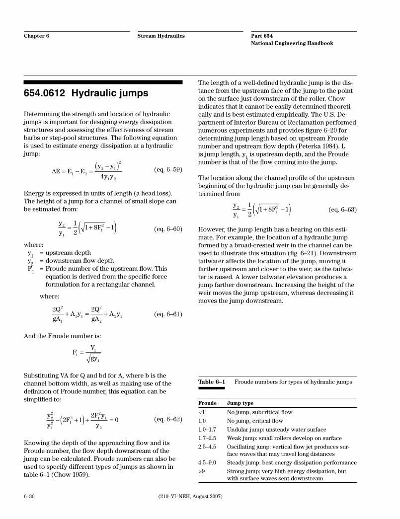
6–30 (210–VI–NEH, August 2007)



654.0612 Hydraulic jumps

Determining the strength and location of hydraulic jumps is important for designing energy dissipation structures and assessing the effectiveness of stream barbs or step-pool structures. The following equation is used to estimate energy dissipation at a hydraulic jump:

∆E E Ey y

y y= − =

−( )1 2

2 1

2

1 24 (eq. 6–59)

Energy is expressed in units of length (a head loss). The height of a jump for a channel of small slope can be estimated from:

y

yF1

22

1

1

21 8 1= + −( ) (eq. 6–60)

where:y

1 = upstream depth

y2 = downstream flow depth

F1 = Froude number of the upstream flow. This

equation is derived from the specific force formulation for a rectangular channel.

where:

2 2

11

22

Q

gAA y

Q

gAA y

2

1

2

2+ = + (eq. 6–61)

And the Froude number is:

FV

gy1

1=1

Substituting VA for Q and bd for A, where b is the channel bottom width, as well as making use of the definition of Froude number, this equation can be simplified to:

y

yF 1

F y

y22

12 1

2 12

− +( ) + =22

01

2

(eq. 6–62)

Knowing the depth of the approaching flow and its Froude number, the flow depth downstream of the jump can be calculated. Froude numbers can also be used to specify different types of jumps as shown in table 6–1 (Chow 1959).

The length of a well-defined hydraulic jump is the dis-tance from the upstream face of the jump to the point on the surface just downstream of the roller. Chow indicates that it cannot be easily determined theoreti-cally and is best estimated empirically. The U.S. De-partment of Interior Bureau of Reclamation performed numerous experiments and provides figure 6–20 for determining jump length based on upstream Froude number and upstream flow depth (Peterka 1984). L is jump length, y

1 is upstream depth, and the Froude

number is that of the flow coming into the jump.

The location along the channel profile of the upstream beginning of the hydraulic jump can be generally de-termined from

y

yF1

22

1

1

21 8 1= + −( ) (eq. 6–63)

However, the jump length has a bearing on this esti-mate. For example, the location of a hydraulic jump formed by a broad-crested weir in the channel can be used to illustrate this situation (fig. 6–21). Downstream tailwater affects the location of the jump, moving it farther upstream and closer to the weir, as the tailwa-ter is raised. A lower tailwater elevation produces a jump farther downstream. Increasing the height of the weir moves the jump upstream, whereas decreasing it moves the jump downstream.

Table 6–1 Froude numbers for types of hydraulic jumps

Froude Jump type

<1 No jump, subcritical flow

1.0 No jump, critical flow

1.0–1.7 Undular jump: unsteady water surface

1.7–2.5 Weak jump: small rollers develop on surface

2.5–4.5 Oscillating jump: vertical flow jet produces sur-face waves that may travel long distances

4.5–9.0 Steady jump: best energy dissipation performance

>9 Strong jump: very high energy dissipation, but with surface waves sent downstream

6–31(210–VI–NEH, August 2007)



Figure 6–20 Determination of jump length based on upstream Froude number

160

150

140

130

120

110

100

90

80

70

60

50

40

30

20

10

0

L/y

1

Froude number

0 2 4 6 8 10 12 14 16 18 20

Sec 2

Sec 3

P3W

θ

Q

P2

L

Figure 6–21 Parameters involved with modeling a hy-draulic jump

6–32 (210–VI–NEH, August 2007)



However, the weir will not cause an hydraulic jump if it is drowned out by downstream tailwater. The down-stream depth must be less than critical depth over the weir plus the weir height, or, using the definition of critical depth:

yy h

312

3<

+( ) (eq. 6–64)

where:y

1 = depth upstream of the weir

h = weir heighty

3 = tailwater depth downstream

654.0613 Channel routing

Channel routing is an important component of hydro-logic modeling and assessments. Designers need to be able to estimate not only flow volumes, but also hy-draulic parameters for many projects. Efforts to math-ematically model and predict channel routing started with Jean Claude Saint-Venant in 1871. However, it is only with the advent of high speed computers that many of the techniques are readily available to most designers. The practitioner should keep in mind that even the most advanced computer models simplify natural system processes. It is, therefore, important for the modeler to understand the computational pro-cedures used in the model being applied.

(a) Movement of a floodwave

Channel routing is the calculation of the hydraulic parameters of a floodwave as it moves through a chan-nel. The overall movement is typically described with the concepts of celerity and attenuation. Floodwave celerity is the speed at which the floodwave moves down the channel and is primarily a function of the channel slope. The attenuation of a floodwave is the subsidence or flattening of the wave as it moves down the channel. Floodwave attenuation is directly related to the amount of inchannel or riparian storage avail-able.

(b) Hydraulic and hydrologic routing

The movement of a floodwave is governed by the laws of fluid mechanics. The two equations for clear water flow are the conservation of mass, or the continuity equation, and the momentum equation. These two equations are referred to as the Saint-Venant equa-tions. Traditional hydraulic routing involves a numeri-cal solution to these equations as partial differential equations. Therefore, hydraulic routing is viewed as being more physically based than hydrologic routing.

Traditional hydrologic routing typically uses an alge-braic solution to the continuity equation and a rela-tionship between changes in storage in the reach and discharge at the outlet. Hydrologic routing is often based on analogies of stream channels and basins as a

6–33(210–VI–NEH, August 2007)



set of storage reservoirs with appropriate properties. In fact, hydrologic routing equations are often referred to as storage routing equations. As a result, hydrologic modeling is inherently empirically based. Typical hydrologic routing equations include the Muskingum routing and the Reservoir (Puls) routing procedures.

(c) Saint-Venant equations

Most channel routing performed by computer model-ing is based on some simplification of the Saint-Venant equations. These equations provide a very simple mod-el of very complex processes. These equations are:

Continuity

AV

x

y

x

yq

∂∂

+∂∂

+∂∂

=VB Bt

(eq. 6–65)

Momentum

S =Sy

x

V

x

yf o −

∂∂

−∂∂

−∂∂

V

g g t

1 (eq. 6–66)

where:A = cross-sectional flow areaV = average velocity of waterx = distance along channelB = water surface widthy = depth of watert = timeq = lateral inflow per unit length of channelS

f = friction slope

So = channel bed slope

g = gravitational acceleration

The solutions to the momentum and continuity equa-tions concurrently define the propagation of a flood-wave with respect to distance along the channel and time. Assumptions for these equations include:

• The momentum and continuity equations are shown for one-dimensional flow in the down-stream direction. The natural variation in veloc-ity with respect to depth is ignored. In addition, these equations do not directly address lateral or vertical stream flows that would require a more complex equation.

• Flow is gradually varied so that hydrostatic pressure prevails, and vertical accelerations can be ignored.

• The effects of boundary friction and turbulence can be treated with resistance laws, as they are in steady flow.

• Fluid is incompressible and has a constant density.

(d) Simplifications to the momentum equation

Depending on the relative importance of the various terms of the Momentum equation, it can be simplified for different applications as follow:

Steady uniform flow (kine-matic wave approximation)

S =Sf o

Steady nonuniform flow (diffusive wave approxima-tion)

S =Sy

xf o −∂∂

Steady nonuniform flow(Quasi-steady state dynam-ic wave approximation)

S =Sy

x

V

xf o −∂∂

−∂∂

V

g

Steady nonuniforn flow (full dynamic wave ap-proximation)

S =Sy

x

V

x

yf o −

∂∂

−∂∂

−∂∂

V

g g t

1

Since simplification means that some aspect is being ignored, it is important for a modeler to understand the basis of the model being applied to answer a hydraulic or hydrologic question. Further discussion on application and limitations of some of routing ap-proaches that are used in many computer programs follows.

• Kinematic wave approximation—The ki-nematic wave approximation assumes that the gravitational and frictional forces are in balance. The kinematic wave approximation works best when applied to steep (0.0019, 10 ft/mi or greater), well-defined channels, where the floodwave is gradually varied. Changes in depth and velocity with respect to time and distance are small in magnitude when com-pared to the bed slope of the channel. The approach is often applied in urban areas be-cause the routing reaches are generally short and well defined (circular pipes, concrete lined channels). However, the equations do not allow for hydrograph diffusion, but only simple trans-lation of the hydrograph in time.

6–34 (210–VI–NEH, August 2007)



The application of the kinematic wave equation is limited to flow conditions that do not demon-strate appreciable hydrograph attenuation. This may be an issue in wide channels, since attenu-ation increases with valley storage. The kine-matic wave equations cannot handle backwater effects, since with a kinematic model flow disturbances can only propagate in the down-stream direction.

• Modified Puls reservoir routing—This ap-proach accounts for the difference of inflow as storage over some defined time period. This method is appropriate if lateral storage is the primary physical mechanism that affects the flood routing. This method disregards the equa-tion of motion by focusing on continuity. It is closely related to level pool reservoir routing.

• Muskingum river routing—The Muskingum river routing method is based on two equations. The first is the continuity equation, and the second is a relationship of storage, inflow, and outflow of the reach. This method is based on a weighted function of the difference of inflow as storage over some defined time period. Typi-cally, the coefficients of the Muskingum meth-od are not directly related to physical channel properties and can only be determined from stream gage data.

• Diffusive wave approximation—The diffusion wave model is a significant improvement over the kinematic wave model because of the inclu-sion of the pressure differential term in the momentum equation. This term allows the dif-fusion model to describe the attenuation (dif-fusion effect) of the floodwave. It also allows the specification of a boundary condition at the downstream extremity of the routing reach to account for backwater effects. It also allows the specification of a boundary condition at the downstream extremity of the routing reach to account for backwater effects. Since it does not use the inertial terms (last two terms) from the full momentum equation, it is limited to slowly to moderately rising floodwaves in flat channels (Fread 1982). However, most natural flood-waves can be described with the diffusion form of the equations.

• Muskingum-Cunge—The theoretical develop-ment of the Muskingum-Cunge routing equation is based on the simplification of the convective diffusion equation. In the Muskingum-Cunge formulation, the amount of diffusion is con-trolled by forcing the numerical diffusion to match the physical diffusion represented by the convective diffusion equation. This approach accounts for hydrograph diffusion based on physical channel properties and the inflowing hydrograph. The method includes the conti-nuity equation and a relationship of storage, inflow, and outflow of the reach. The solution is independent of the user-specified computation interval. The coefficients of the Muskingum-Cunge method are based on data such as cross section and estimated Manning’s n and are more physically based than the Muskingum method. Therefore, the Muskingum-Cunge method can be applied to ungaged streams. However, it cannot account for backwater ef-fects, and the method begins to diverge from the full unsteady flow solution when very rap-idly rising hydrographs are routed through flat channel sections.

• Quasi-steady dynamic wave approxima-tion—The third simplification of the full dynamic wave equations is the quasi-steady dynamic wave approximation. In the case of flood routing, the last two terms in the momen-tum equation are often opposite in sign and tend to counteract each other. By including the convective acceleration term and not the local acceleration term, an error is introduced. This error is of greater magnitude than the error that results when both terms are excluded, as in the diffusion wave model. This approach is not often used in flood routing.

• Dynamic wave equations—The dynamic wave equations can be applied to a wide range of one-dimensional flow problems, such as dam break flood wave routing, tidal fluctuations, canal distribution, and forecasting water sur-face elevations and velocities in a river system during a flood. Solution of the full equations is normally accomplished with an explicit or implicit finite difference technique. The equa-tions are solved for incremental times (dt) and incremental distances (dx) along the waterway.

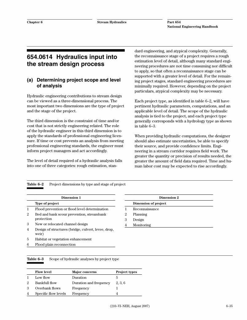
6–35(210–VI–NEH, August 2007)



654.0614 Hydraulics input into the stream design process

(a) Determining project scope and level of analysis

Hydraulic engineering contributions to stream design can be viewed as a three-dimensional process. The most important two dimensions are the type of project and the stage of the project.

The third dimension is the constraint of time and/or cost that is not strictly engineering related. The role of the hydraulic engineer in this third dimension is to apply the standards of professional engineering licen-sure. If time or cost prevents an analysis from meeting professional engineering standards, the engineer must inform project managers and act accordingly.

The level of detail required of a hydraulic analysis falls into one of three categories: rough estimation, stan-

dard engineering, and atypical complexity. Generally, the reconnaissance stage of a project requires a rough estimation level of detail, although many standard engi-neering procedures are not time consuming nor difficult to apply, so that often a reconnaissance stage can be supported with a greater level of detail. For the remain-ing project stages, standard engineering procedures are minimally required. However, depending on the project particulars, atypical complexity may be necessary.

Each project type, as identified in table 6–2, will have pertinent hydraulic parameters, computations, and an applicable level of detail. The scope of the hydraulic analysis is tied to the project, and each project type generally corresponds with a hydrology type as shown in table 6–3.

When providing hydraulic computations, the designer should also estimate uncertainties, be able to specify their source, and provide confidence limits. Engi-neering in a stream corridor requires field work. The greater the quantity or precision of results needed, the greater the amount of field data required. Time and hu-man labor cost may be expected to rise accordingly.

Table 6–2 Project dimensions by type and stage of project

Dimension 1

Type of project

1 Flood prevention or flood level determination

2 Bed and bank scour prevention, streambank protection

3 New or relocated channel design

4 Design of structures (bridge, culvert, levee, drop, weir)

5 Habitat or vegetation enhancement

6 Flood plain reconnection

Dimension 2

Dimension of project

1 Reconnaissance

2 Planning

3 Design

4 Monitoring

Table 6–3 Scope of hydraulic analyses by project type

Flow level Major concerns Project types

1 Low flow Duration 5

2 Bankfull flow Duration and frequency 2, 3, 6

3 Overbank flows Frequency 1

4 Specific flow levels Frequency 4

6–36 (210–VI–NEH, August 2007)



(b) Accounting for uncertainty and risk

The hydraulic engineer must always keep in mind the level of certainty inherent in data measurements, computational methods, and information provided by others. For example, the frequency of flows developed by a hydrologist is, at best, a statistical derivation with confidence limits. The hydraulic engineer can inspect the steepness of the frequency curve, as well as the confidence limits to determine the range of flows that should be associated with a given recurrence inter-val. If the hydrologist had no gage data from which to develop frequency information, the hydrology would probably be considered even less reliable.

As described in this chapter, numerous methods in hydraulic engineering were developed from empirical studies. The designer should know what situations are and are not applicable to a given methodology. When-ever simplified methods are employed, the designer should be aware of the sacrifice in confidence of results.

One typical response in the attempt to minimize the risk due to uncertainty is to use factors of safety and be conservative. However, it is critical that the designer apply factors of safety to the correct calcu-lations and be conservative in the correct aspect of the analysis. To be conservative from a flood control perspective is to design a larger than necessary chan-nel. However, if the goal of the project is to reconnect the flood plain, that designer’s conservatism may lead to design failure.

The designer should keep track of each computational attempt to account for uncertainty. In each case, an adjustment should be justified by a description of the source of the uncertainty and reasoning regarding the magnitude of the adjustment. In many cases, a conven-tional factor of safety will have been established by the field of hydraulic engineering. Standard freeboard heights for channel design are also conventional.

Finally, the hydraulic engineer may wish to more fully document the impact of uncertainties by modeling what-if scenarios, considering extreme values of one or more parameters.

654.0615 Conclusion

This chapter provided an overview of the hydraulic en-gineering concepts involved in stream design. A num-ber of typical hydraulic computations were provided as examples. This discussion can help all disciplines better understand the role of hydraulics in the stream design process.

chapter 6 – stream hydraulics

Documents