
34

The open-channel hydraulics is a foundation of river engineering, hydropower engineering,

irrigation and drainage, and water works (water supply), and underwater engineering. It

describes fluid mechanics related with water flows over a fixed boundary. This means the

container that conveys water is not deformed due to erosion or sediment deposition. Therefore,

no sediment transport by the flow is not considered in this chapter.

1. Introduction

1.1 Laminar and turbulent flows

Pipe flow is thought to be critical when its Reynolds number reaches 2000. The same value

can be applied to an open-channel flow by substituting the hydraulic radius for the

characteristic length in the Reynolds number. That is, the Reynolds number in open-channel is

defined as

Re hVRν

= (1)

where V = characteristic velocity, Rh = hydraulic radius and ν = kinematic viscosity. In open-

channel flows, by using 4 hD R= (here, D = pipe diameter), the flow is laminar when Re <

500, transitional when 500 < Re < 2000, and turbulent when Re > 2000. Particularly, in an

open-channel, the laminar flow is hardly observed in nature unless it is made artificially (for

example, a thin film of liquid flowing down an inclined or vertical plane).

1.2 Subcritical and supercritical flows

The Froude number defined below represents the relative magnitude of the inertia force to the

gravity force (strictly speaking, the Froude number denotes the square root of the ratio of the

inertia force to the gravity force)


35

VFrgD

= (2)

where D = hydraulic depth. This dimensionless number has generally little aerodynamic

interest, but it is of considerable importance in ship design, where gravitational (wave) force is

the primary determinant of the total forces.

(Q) What is the Froude number for large slope angle θ and for α ≠ 0 ?

𝐹𝐹𝐹𝐹 = 𝑉𝑉�𝑔𝑔𝑔𝑔cos𝜃𝜃/𝛼𝛼

In Eq.(2), V is the flow velocity and �𝑔𝑔𝑔𝑔 is the celerity (wave speed) of the longwave. Under

a critical condition, i.e., Fr = 1, the flow velocity is the same as the celerity of the long wave.

(1) Fr < 1: Subcritical Flow

Flow velocity is less than the celerity of the long wave. Any disturbance made at the

downstream point propagates at a speed of �𝑔𝑔𝑔𝑔 − 𝑉𝑉 in the upstream direction. So the

downstream influences the upstream.

(2) Fr > 1: Supercritical Flow

Flow velocity is greater than the celerity of the long wave. Any disturbance made at the

downstream cannot be transmitted in the upstream direction.

2. Basic Properties

2.1 Longitudinal profiles

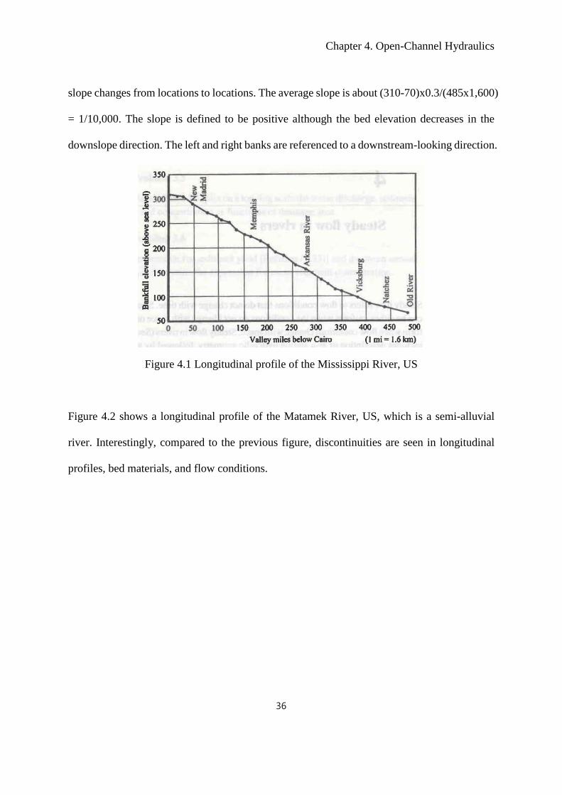
Figure 4.1 shows a longitudinal profile of the Mississippi River, US. It can be seen that the


36

slope changes from locations to locations. The average slope is about (310-70)x0.3/(485x1,600)

= 1/10,000. The slope is defined to be positive although the bed elevation decreases in the

downslope direction. The left and right banks are referenced to a downstream-looking direction.

Figure 4.1 Longitudinal profile of the Mississippi River, US

Figure 4.2 shows a longitudinal profile of the Matamek River, US, which is a semi-alluvial

river. Interestingly, compared to the previous figure, discontinuities are seen in longitudinal

profiles, bed materials, and flow conditions.


37

Figure 4.2 Longitudinal profile of the Matamek River, US


38

2.2 Cross section properties

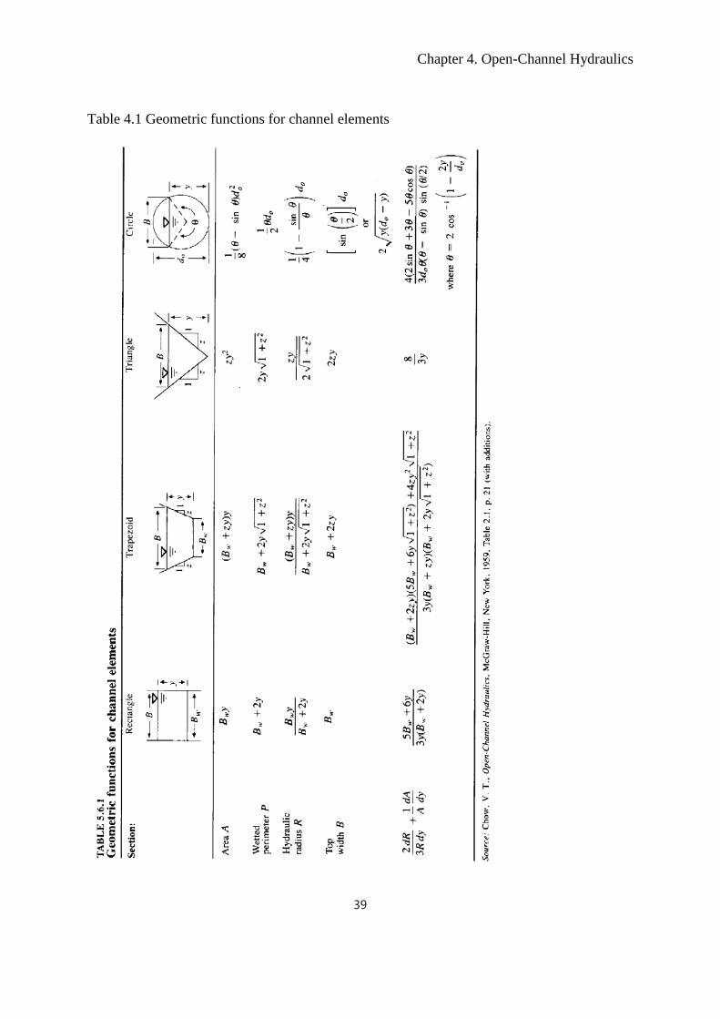
For a cross section of an open channel, the following geometric elements are defined:

▪ flow depth (y): the vertical distance of the lowest point of a channel section from the free

surface

▪ stage: the elevation of the free surface above a datum

▪ top width (T): the width of channel section at the free surface

▪ water area (A): the cross sectional area of the flow normal to the flow of direction

▪ wetted perimeter (P): the length of the line of intersection of the channel wetted surface

with a cross sectional plane normal to the flow direction. The wetted perimeter is related to

the shear stress acting in the opposite direction of the flow

▪ hydraulic radius (Rh): the ratio of the water area to its wetted perimeter

hARP

=

▪ hydraulic depth (D): the ratio of the water area to the top width

D = A ∕ T

▪ section factor for critical flow computation (Z):

Z = A√𝑔𝑔

▪ prismatic channel: a channel with unvarying cross-section and constant slope


39

Table 4.1 Geometric functions for channel elements


40

Figure 4.3 shows a cross section of a river. The top width (T) is 53.0 m, and the wetted

perimeter (P) is 53.3 m. The water area (A) is 45.9 m2. The hydraulic depth (D: mean flow

depth) is 0.87 m, and the hydraulic radius ( hR ) is 0.86 m. The cross section of the river is a

wide open channel since the width to depth ratio exceeds 10 – 15. For such wide open channels,

the hydraulic radius is very close to the mean flow depth.

Figure 4.3 Cross section of a river

2.3 Velocity distributions

Most flows in the river are hydraulically-rough flows without the viscous sublayer. Then the

logarithmic velocity law can be applied to those flows.

*

( ) 1 1ln 8.5 ln 30s s

u z z zu k kκ κ

= + =

(3)

where sk is the effective roughness height. If one integrates Eq.(3) over the depth, he can

obtain the relation such as


41

*

1 1 1ln 8.5 ln 11s

H

ks s

U z Hdzu H k kκ κ

= + =

∫ (4)

where U is the depth-averaged velocity. This relation is called Keulegan’s resistance relation

for rough flow. An approximation to Keulegan’s relation is the Manning-Strickler power form

such as

1/6

*

8.1s

U Hu k

=

(5)

Figure 4.4(a) and 4.4(b) show velocity distributions in the vertical and transverse directions,

respectively. From Figure 4.4(a), the unit discharge can be estimated by

q = 0.55 x 1.0 + 0.85 x 1.0 + 1.0 x 1.0 + 1.1 x 0.7 = 3.17 ft2/s

which is the discharge per unit width. Since the flow depth is 3.7 ft, the depth-averaged velocity

is given by

/ /U Q A q H= = = 0.86 ft/s.

Figure 4.4(b) shows the lateral distribution of the flow depth as well as the depth-averaged

velocity. The figure indicates that the velocity is faster at the middle part of the channel, where

the depth is deeper, in a relatively straight reach.


42

Figure 4.4 Velocity distributions

Example 4.1 Velocity distribution

Consider measured velocity profile in Figure 4.5(a). Measured velocities at tow heights are 1u =

0.168 m/s at 1z = 0.15 m and 2u = 0.250 m/s at 2z = 0.457 m. The river is 60 m wide.

(1) Find the shear velocity.

Using the relationship given by Eq.(3), we have

* 11 *ln 8.5

s

u zu ukκ

= +

* 22 *ln 8.5

s

u zu ukκ

= +

which leads to


43

* 2 * 1 * 22 1

1

ln ln lns s

u z u z u zu uk k zκ κ κ

− = − =

Therefore, we have

( ) ( )

( )2 1

*2 1

0.41 0.25 0.168ln( / ) ln 0.457 / 0.15

u uu

z zκ − × −

= =

= 0.03 m/s

(2) Find the bed shear stress

The bed shear stress is given by

2 2* 1,000 0.03b uτ ρ= = ×

= 0.9 Pa

2.4 Rating curve

The stage-discharge relationship is called “rating curve.” The idea of the rating curve might

come from the convenience of predicting the discharge for a given stage. This relation is unique

for the uniform flow. That is, the discharge is proportional to the power of 5/3 of the flow depth

if the Manning’s formula is used. However, except for the uniform flow, the rating curve shows

a loop. That is, during a particular flood event, the number of stages are two for a discharge.

The stage is higher for the falling limb, indicating the velocity is lower in the falling stage of

the flood than in the rising stage.

The rating curve might be unique for channels with fixed beds. However, for channels with

mobile beds, the rating curve shifts over time because bed aggradation or degradation and


44

changes in bedforms.

Figure 4.5 Rating curves


45

3. Uniform Flows

Depending on the temporal variability (at a particular distance), the open-channel flows are

divided into steady flows and unsteady flows. Similarly, depending on the spatial variability

(at a particular time), the flows can be divided into uniform flows and non-uniform flows. Thus,

we have four combinations as

▪ steady uniform flows

▪ steady non-uniform flows

▪ unsteady uniform flows

▪ unsteady non-uniform flows

Since the flows which are unsteady with time cannot be uniform with distance, the unsteady

uniform flows do not exist. We simply call steady uniform flows as uniform flows, steady non-

uniform flows as non-uniform flows, and unsteady non-uniform flows as unsteady flows.

3.1 Characteristics of uniform flows

Uniform flows in the open channel are defined by

(1) the flow depth, water area, velocity, and discharge at every section of the channel reach are

constant

(2) the slope of energy line ( eS ), the slope of water surface (Sw), and the slope of the channel

bottom (So) are the same

As stated, uniform flows are considered to be steady only because unsteady uniform flows are

practically nonexistent.

A constant velocity may be interpreted as a constant mean velocity. This should mean that the


46

flow possesses a constant velocity at every point on the channel section within the channel

reach. That is, the velocity distribution across the channel section is unaltered in the reach.

Such a stable pattern is attained when the boundary layer is fully developed.

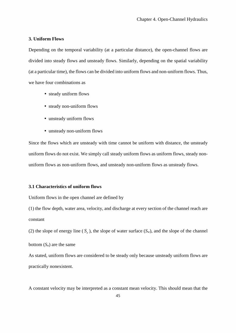
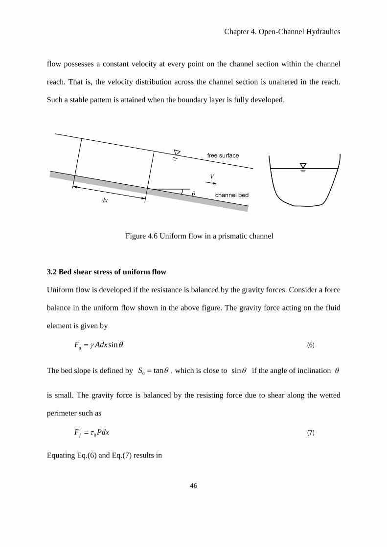
Figure 4.6 Uniform flow in a prismatic channel

3.2 Bed shear stress of uniform flow

Uniform flow is developed if the resistance is balanced by the gravity forces. Consider a force

balance in the uniform flow shown in the above figure. The gravity force acting on the fluid

element is given by

singF Adxγ θ= (6)

The bed slope is defined by 0 tanS θ= , which is close to sinθ if the angle of inclination θ

is small. The gravity force is balanced by the resisting force due to shear along the wetted

perimeter such as

0fF Pdxτ= (7)

Equating Eq.(6) and Eq.(7) results in


47

0 0hR Sτ γ= (8)

where 0S denotes the channel slope ( = sin θ). Note that 0 w eS S S= = for uniform flows.

3.3 Uniform flow formulas

3.3.1 Chezy formula

In 1769, a French engineer named Antoine de Chezy proposed the following relationship for

the velocity V in the open-channel:

h oV C R S= (9)

where C = Chezy coefficient, Rh = hydraulic radius, and So = bed slope. Eq.(9) is an empirical

formula, made using data collected in canals in Paris. According to Chezy’s formula, the mean

velocity is proportional to the square root of the hydraulic radius and bed slope.

In fluid mechanics, the bed shear stress is represented by

20

12fC Vτ ρ= (10)

where fC is the flow resistance coefficient. Using Eq.(7), the resisting force by the bed shear

stress can be expressed as

2fF KV Pdx= (11)

where K is a proportionality. Using Eqs.(6) and (11), a relationship similar to Chezy’s formula

can easily be obtained with C = �𝛾𝛾/𝐾𝐾.


48

3.3.2 Manning formula

Robert Manning was an engineer for the arterial drainage and inland navigation in Office of

Public Works in Ireland. In 1889, for estimating the discharge in the open channel easily, he

compared seven formulas with collected data and proposed the following relationship:

2/3 1/20

1hV R S

n=

where n = roughness coefficient. This relationship is different from Chezy’s in that the velocity

is proportional to 2/3hR , not to 1/2

hR . Note that both Chezy’s and Manning’s formulas are

dimensionally non-homogeneous. For this, the following remedy is used:

2/3 1/20

mh

CV R Sn

= (12)

where the value of Cm is 1 and 1.49 for SI and English units, respectively. The following Table

delivers representative Manning’s roughness coefficients for various boundary materials.

Table 4.2 Manning’s roughness coefficients


49

3.3.3 Darcy-Weisbach formula

The Darcy-Weisbach formula has a long historical background (Brown, 2003). In 1845,

Weisbach proposed the following relationship for the head loss:

2

2LL Vh fD g

=

where f is the friction factor. If the above relationship is rewritten for the velocity with the

use of hR , then we have

08

hgV R Sf

= (13)

At that time when Weisbach proposed the above relationship, the friction factor was not well

defined. In 1857, Darcy suggested that the friction factor is related not only the wall roughness

but also the pipe diameter. Later, Rouse proposed a curve for the friction factor in 1943, which

was further improved by Moody in 1944. While the formula is named after two great engineers

of 19-th century, many others have also aided in the effort.

In general, the friction factor f is

f = fn (ε ∕R, Re) (14)

in which ε is the roughness height. Values of roughness coefficient f are given in the Moody

diagram which is obtained from experiments of pipe flows. The expressions for f are

f = 24Re

Re ≤ 500 (15a)

f = 0.223Re1/4 500 < Re ≤ 25,000 (15b)

For fully-developed turbulent flows over hydraulically-smooth boundary with Re > 25,000,


50

1�𝑓𝑓

= 2logRe�𝑓𝑓 + 0.4 (16a)

and for fully-developed turbulent flows over hydraulically-rough boundary with u*k∕ν > 70 or

Re�𝑓𝑓∕(R∕k) > 50,

1�𝑓𝑓

= 2log 𝑅𝑅𝑘𝑘

+ 2.16 25,000 < Re (16b)

where k is the equivalent size of the Nikuradse type surface roughness and u* is the shear

velocity (= �𝜏𝜏0/𝜌𝜌).

Among three resistance factors, the Darcy-Weisbach f has the best theoretical background. It

is non-dimensional and its values for steady uniform flows are given in the Moody diagram.

However, it should be emphasized that the roughness coefficient f in Darcy-Weisbach formula

is a local quantity as indicated by the above relationship whereas the roughness coefficients of

the other formulas are reach-averaged quantities. The reason why Darcy-Weisbach formula is

not so popular in the practical hydraulics is that the roughness coefficient comes from the pipe

flow experiments. That is, there is no Moody diagram for the open-channel flow, and f-Re

relationship changes according to channel geometry.

3.4 Dimensional consideration

The uniform flow formulas can be expressed as

0 fS S= (17)

which states that the friction slope, defined by ( )0 /f hS Rτ γ≡ from Eq.(8), is the same as

the bed slope. In Eq.(17), the friction slope is given by


51

2

2fh

VSC R

= if Chezy’s formula is used

2 2

4/3fh

n VSR

= if Manning’s formula is used

2

8fh

fVSgR

= if Darcy-Weisbach’s formula is used

Manning’s, Chezy’s, and Darcy-Weisbach’s formulas were originally developed empirically

although theoretical numerous attempts were made later. From the three relationships, it is

clear that

1/68 m hC RC

f ng g= = (18)

The above equation reveals that

(a) The Chezy C has the dimension of �𝑔𝑔.

(b) Cm in the Manning’s formula has the dimension of �𝑔𝑔 because it is unreasonable to

assume n changes with changing g. Therefore, the Manning’s n has the dimension of [L1/6].

Although n has a dimension of [L1/6], in practice the same numerical value of n is used in

English system as in SI system, and hence the constant 1.49 absorbs not only the dimension of

g but also the conversion factor from SI system.

Example 4.2: Uniform flow

Consider a steady flow of Q = 10 𝑚𝑚3/s in a 10 m wide rectangular channel. The slope of the


52

channel is 0S = 0.26/1,000 and the friction factor is f = 0.01.

(1) Find the normal depth ny of the flow.

The mean velocity by Darcy-Weisbach formula is given by

08

hgV R Sf

=

Here, hR y for wide channels. Therefore, the unit discharge is given by

3/2 1/2

08

ngq y Sf

=

Thus, we have

3/2 1/2

08nfy q Sg

−=

=

1/210 0.01 0.2610 8 9.8 1,000

− × × ×

= 0.70

Therefore, the normal depth is

ny = 0.79 m

If we do not assume that the channel is wide, then the hydraulic radius is

2n

hn

WyRW y

=+

= 0.68 m.

which is 14% smaller than the flow depth.

(2) Find Manning’s n and Chezy’s C.

Using the relationship given by Eq.(18), we have


53

8 88gCf

= =

1/6

0.0118

hf Rn

g= =

(3) Find the bed shear stress

The bed shear stress is calculated as

0 0 9,801 0.681 0.00026hR Sτ γ= = × ×

= 1.74 Pa

4. Energy and Momentum Principles

The energy equation derived in the fluid mechanics can hardly be applied to open-channel

flows since the pressure varies vertically. Thus the energy principle, specific energy, tailored

specially for open-channel flows, is used. Similarly, the specific force is the momentum

principle simplified and devised only for open-channel flows.

4.1 Energy principle

4.1.1 Specific energy

Applying the energy equation at two points shown in the figure below leads to the following

relationship:

2 2

1 1 2 21 1 2 22 2 L

p V p Vz z hg g

α αγ γ+ + = + + + (19)

where


54

11 1 0

p z y x Sγ+ = + ∆ ⋅ ; 2

2 2p z yγ+ =

If we assume that α1 = α2 = 1 and 0 0S , then we have

2 2

1 21 22 2

V Vy yg g+ = + (20)

where the head loss is also neglected. It can be seen that the sum of velocity head and water

depth is constant and it is defined as the specific energy. The specific energy is the total energy

per unit weight with elevation datum taken as the bottom of the channel. That is,

2 2

22 2sV QE y y

g gA= + = + (21)

which is constant.

Figure 4.7 Derivation of specific energy

4.1.2 Critical depth

The specific energy has a minimum value below which the given Q cannot occur. The value of

y for minimum sE is obtained by differentiating Eq.(21), i.e.,


55

2 2

31 1sdE Q dA V dAdy gA dy gA dy

= − = − (22)

Near the free surface, it holds that dA/dy = T. Thus,

2 2

21 1 1sdE V T V Frdy gA gD

= − = − = − (23)

where D is the hydraulic depth (D = A/T). Therefore, if the specific energy is minimum for a

given discharge, then it should hold that

2

2 2V D

g= (24)

Since no approximations about the shape of the channel are made in deriving eq.(24), it should

be applied any arbitrary-shaped channel.

For rectangular channels, the critical depth is given by

( )1/32 /cy q g= (25)

Substituting cy into Eq.(21) results in the minimum value of the specific energy such as

Min(𝐸𝐸𝑆𝑆) = 32𝑦𝑦𝑐𝑐 (26)

4.1.3 Critical Slope

In a mild slope condition, the normal depth is higher than the critical depth. As the slope

increases gradually, the normal depth is lowered with the critical depth unchanged. When two

depths become identical, the slope is said to be critical. If the slope is steeper than the critical

slope, it becomes steep slope.


56

The slope of the channel that sustains a given discharge at a uniform and critical depth is called

the critical slope Sc. This slope can be obtained by substituting the velocity from Eq.(12) into

eq.(24)

2

4/3ch

n gDSR

= (27)

Notice that the critical slope is proportional to the squared roughness. That is, the more rough

channel requires the higher slope to be a critical flow for a given discharge. It is interesting to

note that the uniform flow on the mild slope is a subcritical flow but the uniform flow on the

steep slope is a supercritical flow.

4.2 Momentum principle

Consider the control volume of the open-channel flow in the figure below. The momentum

equation applied to the control volume can be written as

( )2 1F Q V Vρ= −∑ (28)

where the LHS of the above equation denotes the sum of the external forces acting on the

control volume. That is,

1 2 sin fF P P W Fθ= − + −∑ (29)

where W is the weight of water in the control volume and fF is the friction. If we ignore both

the weight of water in the control volume and friction, then we have

( )2 1 1 2Q V V P Pρ − = − (30)

or


57

2 2

1 1 2 21 2

g gQ Qh A h AgA gA

+ = + (31)

where gh is the vertical distance from the free surface to the centroid of A. The above equation

shows that the sum of two terms, defined by the specific force, is conserved at two cross

sections. That is, the specific force is defined by

2

gQM h AgA

= + (32)

where the first term represents the momentum per unit time and per unit weight of water and

the second term the hydrostatic force per unit weight of water.

Figure 4.8 Forces acting on the control volume of the open channel flow

If the specific force is differentiated with respect to h, then

( )2

2 gdM Q dA d h Ady gA dy dy

= − + (33)

From / 0dM dy = , one has


58

2

2 2V D

g= (34)

which indicates that the critical flow occurs if the specific force is minimum for a given

discharge.

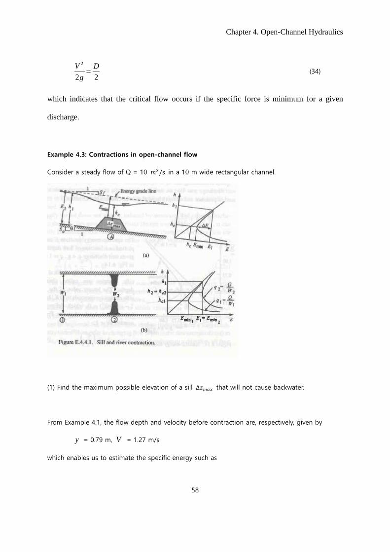
Example 4.3: Contractions in open-channel flow

Consider a steady flow of Q = 10 𝑚𝑚3/s in a 10 m wide rectangular channel.

(1) Find the maximum possible elevation of a sill ∆𝑧𝑧𝑚𝑚𝑚𝑚𝑚𝑚 that will not cause backwater.

From Example 4.1, the flow depth and velocity before contraction are, respectively, given by

y = 0.79 m, V = 1.27 m/s

which enables us to estimate the specific energy such as


59

2

2sVE y

g= + = 0.87 m

Since the unit discharge is /q Q W= = 1.0 m2/s, the critical depth is

1/32

cqyg

=

= 0.467 m

The minimum value of the specific energy is

_ min32s cE y= =0.70 m

Since

_ min maxs sE E z= + ∆

Therefore, the maximum elevation of the sill is given by

maxz∆ = 0.17 m

(2) Find the maximum lateral contraction ∆𝑊𝑊𝑚𝑚𝑚𝑚𝑚𝑚 of the channel that will not cause backwater.

Since 3 / 2s cE y= , the critical depth and velocity are, respectively, by

23c sy E= = 0.58 m

cV gy= = 2.39 m/s

The width required to deliver Q is given by

' / ( )cW Q y V= × = 7.21 m

Therefore, the maximum lateral contraction is calculated as

max 'W W W∆ = − = 2.79 m


60

5. Rapidly Varied Flows (Hydraulic Jump)

From a practical viewpoint, hydraulic jump is a useful means of dissipating excess energy of

supercritical flows. Its merit is in preventing possible erosion below overflow spillways, chutes,

and sluices, for it quickly reduces the velocity of the flow on a paved apron to a point where

the flow becomes incapable of scouring the downstream channel bed. The hydraulic jump used

for energy dissipation is usually confined partly or entirely to a channel reach that is known as

the stilling basin. The bottom of the basin is paved to resist scouring. Hydraulic jump can also

be used as mixing devices for the addition and mixing of chemicals in water and wastewater

treatment plants. In natural channels, a hydraulic jump is used to provide aeration of the water

for environmental considerations.

Hydraulic jump in a horizontal plane is considered herein. From the continuity relationship,

1 1 2 2V y V y= (35)

and, from the momentum equation

𝛾𝛾𝑦𝑦12

2− 𝛾𝛾𝑦𝑦22

2= 𝜌𝜌𝑉𝑉2(𝑦𝑦2𝑉𝑉2) + 𝜌𝜌𝑉𝑉2(−𝑦𝑦1𝑉𝑉1) (36)

Solving the above two equations together leads to

𝑦𝑦2 = −𝑦𝑦12

+ 𝑦𝑦12�1 + 8𝐹𝐹𝐹𝐹12 (37)

or

𝑦𝑦2𝑦𝑦1

= 12��1 + 8𝐹𝐹𝐹𝐹12 − 1� (38)

where the depths y1 and y2 are referred to as conjugate depths. Using eq.(38) from the

information before the jump, the water depth after the jump (after the energy dissipation) can

be obtained. Energy is not conserved before and after the jump. In order to obtain the energy


61

loss, the following energy equation should be solved:

𝑉𝑉12

2𝑔𝑔+ 𝑦𝑦1 = 𝑉𝑉22

2𝑔𝑔+ 𝑦𝑦2 + ℎ𝑙𝑙 (39)

where hl represents losses due to the jump. Eliminating V1 and V2 yields

ℎ𝑙𝑙 = (𝑦𝑦2−𝑦𝑦1)3

4𝑦𝑦1𝑦𝑦2 (40)

(Q) Derive the formula for the hydraulic jump in an inclined channel with a slope θ.

Example 4.4: Hydraulic jump

Consider a steady flow of Q = 10 𝑚𝑚3/s in a 10 m wide rectangular channel. The upstream velocity

𝑉𝑉1 = 4 m/s is rapidly reduced to form a hydraulic jump.

(1) Find the flow depth and velocity after the jump.

Since 𝑉𝑉1 = 4 m/s, the flow depth before the jump is 1y = 0.25 m. Thus, Fr before the jump is

given by

11

1

VFrgy

= = 2.56

which indicates that the flow is supercritical. Using the formula by Eq.(38), we have

( )212 11 8 1

2yy Fr= + − = 0.789 m.

which results in 2V = 1.27 m/s.

(2) Find the force after the jump.

The hydrostatic force after the jump can be calculated as

22

2 2yF Wγ

= × = 30.5 KN


62

Example 4.5: Flow under sluice gate

A sluice gate discharges 10 m3/s in a 10 m wide rectangular channel. The flow depth downstream

of the gate is 𝑦𝑦1 = 0.25 m and rapidly increases to the normal depth of 𝑦𝑦2 = 0.788 m. The hydraulic

jump is located at the toe of the sluice gate.

(1) Find the water level upstream of the sluice gate.

The velocity downstream of the gate (before the jump) can be calculated as

11

100.25 10

QVy W

= =×

= 4 m/s

Therefore, the specific energy before the jump is given by

2 2

11 1

40.252 2sVE y

g g= + = + = 1.06 m

which is the same as the specific energy upstream of the sluice gate. That is,

220

0 00

10.252 2sV QE y

g g y W

= + = +

= 1.06

which is reduced to be the third-order equations such as

3 20 0

11.06 02

y yg

− + =

the solution of which is

0y = 1.0 m

with 0V = 1 m/s.

(2) What is the force acting on the sluice gate?

The momentum equation applied to the sluice gate is written as

( )1 0F Q V Vρ= −∑


63

The LHS of the equation is given by

2 20 12 2

F y W y W Fγ γ= − −∑

where F is the force acting on the sluice gate (->). Thus, we have

( )2 20 1 1 02 2

F y W y W Q V Vγ γ ρ= − − −

( ) ( )2 29.800 10 0.25 1 1,000 10 4 12

= × × − − × × −

= 46,000 – 30,000 = 16,000 N (->)

(3) how much energy is lost in the hydraulic jump?

The velocity after the jump is given by

22

100.788 10

QVy W

= =×

= 1.27 m/s

Therefore, the specific energy after the jump is given by

2 2

22 2

1.270.7882 2sVE y

g g= + = + = 0.87 m

Therefore, the energy lost is

1 2s sE E E∆ = − = 1.06 – 0.87 = 0.19 m

6. Gradually Varied Flows

Gradually varied flow is a steady flow whose depth changes gradually along the length of the

channel. This means two assumptions are involved in the definition, namely steady flow and

hydrostatic pressure distribution. The former suggests that the flow is constant with time, and

the latter that the streamlines are practically parallel.


64

6.1 Governing Equation

Consider a control volume of water column in the next page. The total head (H) is

𝐻𝐻 = 𝛼𝛼 𝑉𝑉2

2𝑔𝑔+ 𝑑𝑑cos𝜃𝜃 + 𝑧𝑧 (41)

where α = energy correction factor, V = mean velocity, d = flow depth, and z = elevation of a

channel bottom from a certain datum. Assuming that α = 1 and the slope is very mild, then

cos 1θ ≈ and d y≈ . Differentiating Eq.(41) with respect to x yields

𝑑𝑑𝑑𝑑𝑑𝑑𝑚𝑚

= 𝑑𝑑𝑑𝑑𝑚𝑚�𝑉𝑉

2

2𝑔𝑔� + 𝑑𝑑𝑦𝑦

𝑑𝑑𝑚𝑚+ 𝑑𝑑𝑑𝑑

𝑑𝑑𝑚𝑚 (42)

Figure 4.9 Flow in a rectangular prismatic open-channel

where


= −𝑆𝑆𝑒𝑒 (43a)


= −𝑆𝑆0 (43b)


65

𝑑𝑑𝑑𝑑𝑚𝑚�𝑉𝑉

2

2𝑔𝑔� = − 𝑄𝑄2

𝑔𝑔𝐴𝐴3𝑑𝑑𝐴𝐴𝑑𝑑𝑦𝑦

𝑑𝑑𝑦𝑦𝑑𝑑𝑚𝑚

= −𝑄𝑄2𝑇𝑇𝑔𝑔𝐴𝐴3


= − 𝑉𝑉2

𝑔𝑔𝑔𝑔𝑑𝑑𝑦𝑦𝑑𝑑𝑚𝑚

(43c)

It should be noted in Eq.(39) that the loss of the total head (dH) is always negative in the flow

direction. Gradually varied flow should imply that the water depth does not change

significantly in order to satisfy dA/dy = T. Therefore, we have

021eS Sdy

dx Fr−

=−

(44)

which describes the variation of the flow depth in a channel of arbitrary shape. Eq.(44) is also

referred to as “backwater equation.”

Here, the equation for the gradually varied flow is derived using the energy approach. However,

the same equation can be obtained using the momentum approach, which may provide a better

insight of the weakness of the governing equation. For example, hydrostatic pressure

distribution, which is extremely critical in practice, cannot be seen in the derivation using the

energy approach.

6.2 Classifications of the Gradually Varied Flow

The backwater equation given in Eq.(44) is not ready for solution. Since the dependent variable

is h, eS and Fr are functions of h, the gradually varied flow equation can be re-written as


= 𝑆𝑆01−(𝑦𝑦𝑛𝑛/𝑦𝑦)10/3

1−(𝑦𝑦𝑐𝑐/𝑦𝑦)3 (45)

if the Manning formula is used, and


= 𝑆𝑆01−(𝑦𝑦𝑛𝑛/𝑦𝑦)3

1−(𝑦𝑦𝑐𝑐/𝑦𝑦)3 (46)

if the Chezy formula is used.


66

6.3 Methods of Computation

Computation of gradually varied flows is important in hydraulic engineering practice. In

general, the methods of computing the gradually varied flow can be grouped as

▪ Direct integration method

▪ Step method

▪ Numerical method

The direct integration method includes Bress method and Chow method. The direct step

method and the standard step method belong to the step method. Since the backwater equation

is nonlinear, such method as the Newton-Raphson method can be used. This approach is called

numerical method


67

Figure 4.10 Various types of non-uniform flows


68

7. Unsteady Flows

The continuity and momentum equations for unsteady flows are, respectively, given by

0y y VV yt x x

∂ ∂ ∂+ + =

∂ ∂ ∂ (47a)

( )0 0eV V yV g g S St x x

∂ ∂ ∂+ + − − =

∂ ∂ ∂ (47b)

This set of equations are called Saint Venant equations or the full-dynamic equations. The

momentum equation consists of the local acceleration (the 1st term), the convective

acceleration (the second term), the pressure force term (the third term), the gravity force term

(the fourth term), and the friction force term (the sixth term).

The set of equations, the continuity and momentum equations, are classified into a second-

order hyperbolic type of PDEs. Two characteristics exist, and they propagate in the upstream

and downstream directions for the subcritical flow. This feature of PDE enables the method of

characteristics to be most accurate and feasible for the solution of the PDE. However, the finite

difference method based on the implicit Preissmann scheme became widely used, as indicated

in Chow et al. (1988).

As stated, the set of equations is called “the full-dynamic equation” since it includes all terms

needed for unsteady flows. This is apparent when compared with such simplified approaches

as kinematic wave or diffusion wave approximations. The kinematic wave model only includes

the gravity force and friction force terms, and the diffusion wave model includes the pressure

force term together with the kinematic wave model.


69

Example 4.6

Starting with the momentum equation for unsteady flows, show that, for a discharge. stages are

different for rising and falling limbs of the flood.

If the both acceleration terms are ignored in the momentum equation, one has

( )0 0fyg g S Sx∂

− − =∂

which can be written as

0yQ K Sx∂

= −∂

where /y x∂ ∂ is positive and negative on the falling and rising stages of a flood, respectively.

For the uniform flow, 0 0Q K S=

Example 4.7

Show that the momentum equation for the unsteady flow becomes the backwater equation if

/ 0V t∂ ∂ = .

If / 0V t∂ ∂ = , then the momentum equation for the unsteady flow becomes

( )0 edV dyV g g S Sdx dx

+ = −

where


70

2 2

212

dV dV V dy dyV Frdx g dx gy dx dx

= = − = −

Therefore, we have

021eS Sdy

dx Fr−

=−

References

Brown, G.O. (2003). The history of the Darcy-Weisbach Equation for pipe flow resistance. In

Environmental and Water Resources History, edited by J.R. Rogers and A.J. Fredrich, ASCE,

pp.34-43. Reston, VA.

Chow, V.T. (1959). Open-Channel Hydraulics. McGraw Hill Book Company, New York,

NY.

Chow, V.T., Maidment, D.R., and Mays, L.W. (1988). Applied Hydrology. McGraw Hill

Book Company, New York, NY.

Julien, P.Y. (2002). River Mechanics, Cambridge University Press, Cambridge, UK.

Sabersky, R.H., Acosta, A.J., and Hauptmann, E.G. (1971). Fluid Flow. Macmillan, New

York, NY.

Problems

1. A trapezoidal channel below conveys a discharge of Q = 10 m3/s. The slope and the roughness

are 0.001 and 0.015, respectively.

(1) Make a proper assumption and obtain a normal depth without iterations.

(2) Obtain a normal depth without any assumption.

(3) Make a proper assumption and obtain a critical depth.


71

(4) Obtain a critical depth without any assumption.

2. Find the normal depth and critical depth if the discharge Q = 0.8 cms in a 0.6 m wide rectangular

channel. The slope and roughness coefficient are S = 0.015 and n = 0.015, respectively. Is the slope

of the channel mild or steep?

3. Consider a flow of unit discharge q = 6 m2/s in a wide channel whose slope is S = 0.0002. The

sediment particles on the bed has an effective roughness height of sk = 0.1 m (Use1/6 / 21.0n d=

and 2.0sk d= ). A dam is located downstream of this channel. Obtain the normal depth and critical

depth for this flow. Which type of water surface profile is expected? Explain why.

4. A rectangular sill with the height of z∆ blocks the flow whose velocity and depth are 1.5 m/s

and 2.5 m, respectively.

(1) Find the flow depth over the sill if z∆ = 0.5 m.

(2) Find the maximum value of z∆ if the sill does not affect upstream flow.


72

5. Show that the critical flow occurs if the specific force is minimum for a given discharge in a

rectangular channel.

6. The hydraulic jump occurs immediately downstream of the sluice gate as shown in the figure

below.

(1) Find the tailwater depth.

(2) Find the force on the sluice gate.

(3) What happens if the tailwater depth is higher than the depth computed in (1). Sketch the flow.

(4) What happens if the tailwater depth is lower than the depth computed in (1). Why? Explain using

the water surface profile H3.

chapter 4. open-channel hydraulics

Documents