Chapter 3Averages and Variations

3.1 Measures of Central Tendency

Mode, Median and Mean

What kind of data will we be able to compute mode, median and mean?

Quantitative data can have a mode, median and mean.

Qualitative data can have a mode.

Mode

The value that occurs most frequently is the mode. Some books describe the mode as the “hump” or local high point in a histogram, which does imply frequency of an answer.

Median

The median of a data set is the middle data value.

To find, order the data from smallest to largest, and the data set in the middle (for a data set of n, the middle position is ) is the median.

Does anyone detect a potential problem?

n 12

Mean

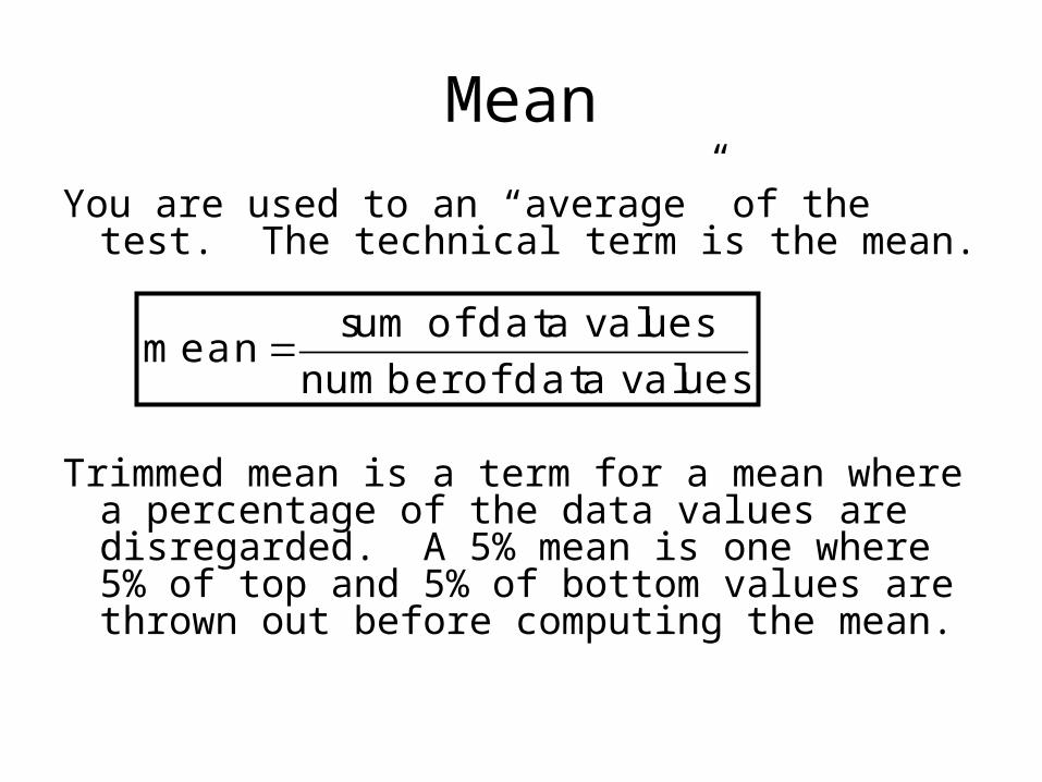
You are used to an “average” of the test. The technical term is the mean.

Mean

You are used to an “average” of the test. The technical term is the mean.

Trimmed mean is a term for a mean where a percentage of the data values are disregarded. A 5% mean is one where 5% of top and 5% of bottom values are thrown out before computing the mean.

sum of data valuesmean

number of data values

Pulse Data

Lets find the mode, the median and the mean of the pulse data from the first day of class.

We just found the population mean (μ) rather than the sample mean ().

What is the difference then between μ and ?

Weighted Averages

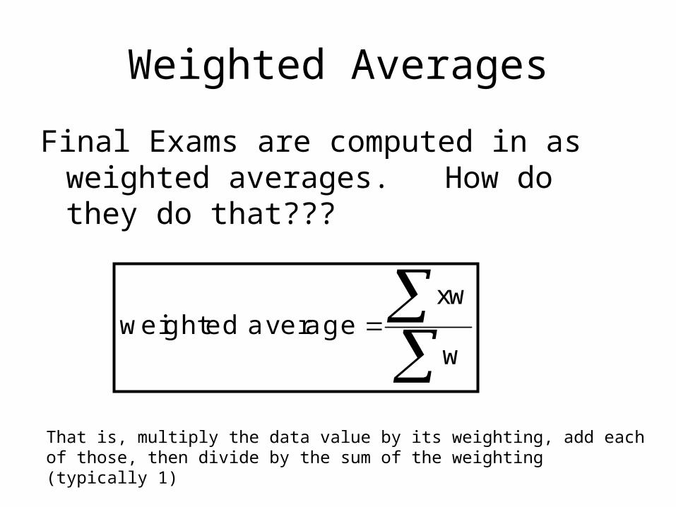
Final Exams are computed in as weighted averages. How do they do that???

Weighted Averages

Final Exams are computed in as weighted averages. How do they do that???

xwweighted average

w

That is, multiply the data value by its weighting, add each of those, then divide by the sum of the weighting (typically 1)

3.2

Measures of Variation

While knowing the mean is important

There is other information from data that you can measure.

These tell you about the spread of the data.

Range – difference between largest and smallest value of a data distribution.

Variance

Variance = measure of how data tends to spread around an expected value (the mean)

Each data point = xMean = Deviation = x – Sample size = nVariance = s2

Standard Deviation = s

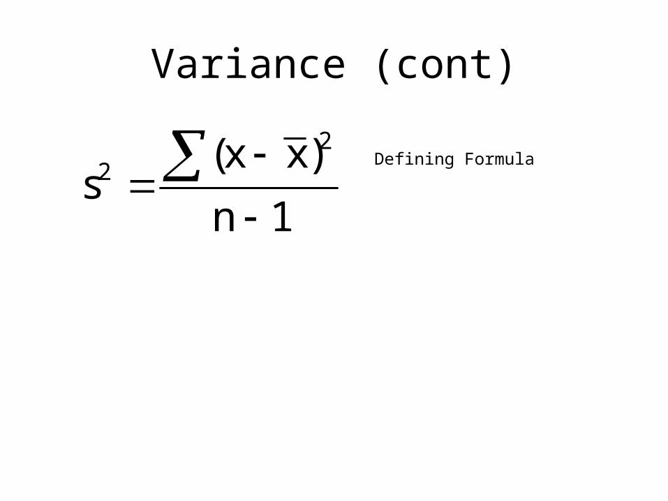
Variance (cont)

22 (x x)

sn 1

Defining Formula

Variance (cont)

22 (x x)

sn 1

Defining Formula

2

2

2

xx

nsn 1

Computation Formula

Variance (cont)

To find standard deviation, just square root the variance.

The computational formula tends to be a little easier to do by hand, but we will practice both.

These two formulas ARE the same.

Variance (cont)

Lets find the variance and the standard deviation of the pulse data, using both formulas.

Variance (cont)

If an entire population is used, instead of a sample, the notation is different but the methods are the same

Each data point = xMean = µDeviation = x – µSample size = NVariance = σ 2

Standard Deviation = σ

Variance (cont)

22 (x )

N

Defining Formula

Variance (cont)

Coefficient of Variance (CV) expresses standard deviation as a percentage of the sample/population mean.

Variance (cont)

Coefficient of Variance (CV) expresses standard deviation as a percentage of the sample/population mean.

sCV 100

x CV 100

Sample Population

Variance (cont)

Chebyshev’s TheoremFor any data set, the proportion that lies

within k standard deviations on either side of the mean is at least

So 75% lies between 2 standard deviations, 88.9% between 3 standard deviations, etc.

2

11

k

3.3 Mean/Standard Deviation

What if you use grouped data

Grouped Data

Lots of data = TEDIOUS, whether you have a calculator or not… If you generally approximate the mean and standard deviation, that sometimes is enough

To deal with this, you actually begin with a frequency table (remember Histograms?

Grouped Data (cont)

1. Make a frequency table2. Find the midpoint of each class = x3. Compute each class frequency = f4. Total number of entries = n

Grouped Data (cont)

1. Make a frequency table2. Find the midpoint of each class = x3. Compute each class frequency = f4. Total number of entries = n

xfaverage x

n

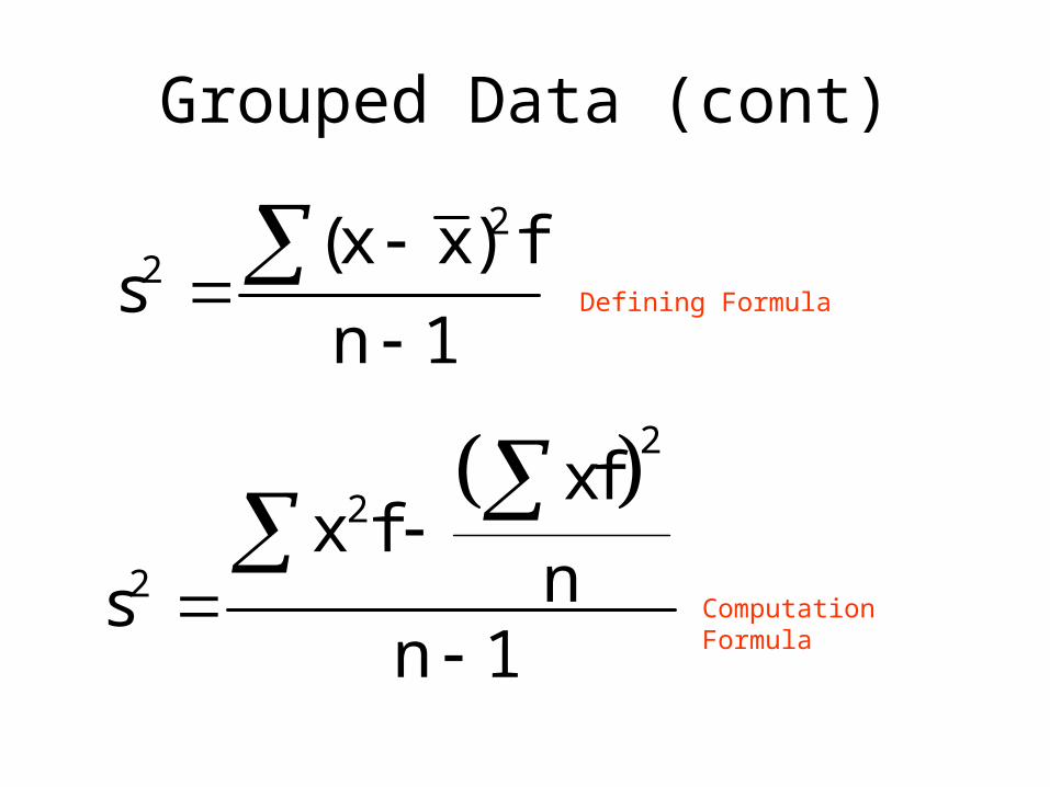
Grouped Data (cont)

22 (x x) f

sn 1

Defining Formula

2

2

2

xfx f

nsn 1

Computation Formula

Grouped Data (cont)

Essentially, by using the midpoint and the frequency, you use a representation for ALL data values in that class, without typing in every data value.

It will be a little off, but again, if the data set is huge it isn’t a bad way to approach the problem.

3.4 Percentiles

Box/Whiskers Plots

Percentiles

Baby Calculator

Children’s BMI

A percentile ranking allows one to know where the particular data value falls in relation to the entire population.

Percentiles (cont)

The Pth percentile (1 ≤ P ≤ 99) is a value so that P% of the data falls at or below it (and 100 – P % falls at/above)

60th Percentile does NOT mean 60% score – it means that 60% of scores fall at or below that position… 60th percentile could be 80%

Where have you seen percentiles?

Percentiles (cont)

Quartiles – special percentiles used frequently. The data is divided into fourths, called Quartiles.

2nd Quartile – Median1st Quartile – Median below (exclude Q2)3rd Quartile – Median above (exclude Q2)Interquartile Range (IQR) = Q3 – Q1

Percentiles (cont)

Lets find the quartiles for following Math class sizes in the 9th grade.

10, 11, 12, 12, 14, 15, 16, 17, 19, 20

Median = 14.5

1st Q = 12

3rd Q = 17

IQR = 17 – 12 = 5

Percentiles (cont)

Lets find the quartile for the pulse data

Why are these values significant? These are needed to make Box and Whiskers Plots

Box and Whiskers Plots

Box and Whiskers Plots (cont)

The five number summary is used to make a box and whisker

plot.

Lets make a box and whiskers plot for the class size data.

Lowest value, Q1, Median, Q3, Highest Value

10

12

14

16

18

20

Lowest Value

Highest Value

Q2

Median

Q1

Box and Whiskers Plots (cont)

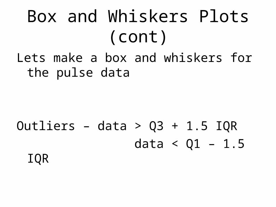
Lets make a box and whiskers for the pulse data

Outliers – data > Q3 + 1.5 IQR data < Q1 – 1.5 IQR

Resources• http://www.statcan.ca/english/edu/power/ch12/plots.htm

• http://www.statsdirect.com/help/graphics/box_whisker.htm

• http://v8doc.sas.com/sashtml/stat/chap18/sect18.htm