Speech and Language Processing. Daniel Jurafsky & James H. Martin. Copyright © 2021. All

rights reserved. Draft of December 29, 2021.

CHAPTER

18 Word Senses and WordNet

Lady Bracknell. Are your parents living?Jack. I have lost both my parents.Lady Bracknell. To lose one parent, Mr. Worthing, may be regarded as amisfortune; to lose both looks like carelessness.

Oscar Wilde, The Importance of Being Earnest

Words are ambiguous: the same word can be used to mean different things. Inambiguous

Chapter 6 we saw that the word “mouse” has (at least) two meanings: (1) a smallrodent, or (2) a hand-operated device to control a cursor. The word “bank” canmean: (1) a financial institution or (2) a sloping mound. In the quote above fromhis play The Importance of Being Earnest, Oscar Wilde plays with two meanings of“lose” (to misplace an object, and to suffer the death of a close person).

We say that the words ‘mouse’ or ‘bank’ are polysemous (from Greek ‘havingmany senses’, poly- ‘many’ + sema, ‘sign, mark’).1 A sense (or word sense) isword sense

a discrete representation of one aspect of the meaning of a word. In this chapterwe discuss word senses in more detail and introduce WordNet, a large online the-WordNet

saurus —a database that represents word senses—with versions in many languages.WordNet also represents relations between senses. For example, there is an IS-Arelation between dog and mammal (a dog is a kind of mammal) and a part-wholerelation between engine and car (an engine is a part of a car).

Knowing the relation between two senses can play an important role in tasksinvolving meaning. Consider the antonymy relation. Two words are antonyms ifthey have opposite meanings, like long and short, or up and down. Distinguishingthese is quite important; if a user asks a dialogue agent to turn up the music, itwould be unfortunate to instead turn it down. But in fact in embedding models likeword2vec, antonyms are easily confused with each other, because often one of theclosest words in embedding space to a word (e.g., up) is its antonym (e.g., down).Thesauruses that represent this relationship can help!

We also introduce word sense disambiguation (WSD), the task of determiningword sensedisambiguation

which sense of a word is being used in a particular context. We’ll give supervisedand unsupervised algorithms for deciding which sense was intended in a particularcontext. This task has a very long history in computational linguistics and many ap-plications. In question answering, we can be more helpful to a user who asks about“bat care” if we know which sense of bat is relevant. (Is the user is a vampire? orjust wants to play baseball.) And the different senses of a word often have differ-ent translations; in Spanish the animal bat is a murcielago while the baseball bat isa bate, and indeed word sense algorithms may help improve MT (Pu et al., 2018).Finally, WSD has long been used as a tool for evaluating language processing mod-els, and understanding how models represent different word senses is an important

1 The word polysemy itself is ambiguous; you may see it used in a different way, to refer only to caseswhere a word’s senses are related in some structured way, reserving the word homonymy to mean senseambiguities with no relation between the senses (Haber and Poesio, 2020). Here we will use ‘polysemy’to mean any kind of sense ambiguity, and ‘structured polysemy’ for polysemy with sense relations.

2 CHAPTER 18 • WORD SENSES AND WORDNET

analytic direction.

18.1 Word Senses

A sense (or word sense) is a discrete representation of one aspect of the meaning ofword sense

a word. Loosely following lexicographic tradition, we represent each sense with asuperscript: bank1 and bank2, mouse1 and mouse2. In context, it’s easy to see thedifferent meanings:

mouse1 : .... a mouse controlling a computer system in 1968.mouse2 : .... a quiet animal like a mousebank1 : ...a bank can hold the investments in a custodial account ...bank2 : ...as agriculture burgeons on the east bank, the river ...

18.1.1 Defining Word SensesHow can we define the meaning of a word sense? We introduced in Chapter 6 thestandard computational approach of representing a word as an embedding, a pointin semantic space. The intuition of embedding models like word2vec or GloVe isthat the meaning of a word can be defined by its co-occurrences, the counts of wordsthat often occur nearby. But that doesn’t tell us how to define the meaning of a wordsense. As we saw in Chapter 11, contextual embeddings like BERT go further byoffering an embedding that represents the meaning of a word in its textual context,and we’ll see that contextual embeddings lie at the heart of modern algorithms forword sense disambiguation.

But first, we need to consider the alternative ways that dictionaries and the-sauruses offer for defining senses. One is based on the fact that dictionaries or the-sauruses give textual definitions for each sense called glosses. Here are the glossesgloss

for two senses of bank:1. financial institution that accepts deposits and channels

the money into lending activities

2. sloping land (especially the slope beside a body of water)

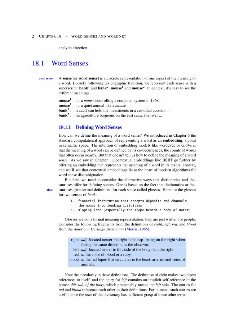
Glosses are not a formal meaning representation; they are just written for people.Consider the following fragments from the definitions of right, left, red, and bloodfrom the American Heritage Dictionary (Morris, 1985).

right adj. located nearer the right hand esp. being on the right whenfacing the same direction as the observer.

left adj. located nearer to this side of the body than the right.red n. the color of blood or a ruby.

blood n. the red liquid that circulates in the heart, arteries and veins ofanimals.

Note the circularity in these definitions. The definition of right makes two directreferences to itself, and the entry for left contains an implicit self-reference in thephrase this side of the body, which presumably means the left side. The entries forred and blood reference each other in their definitions. For humans, such entries areuseful since the user of the dictionary has sufficient grasp of these other terms.

18.1 • WORD SENSES 3

Yet despite their circularity and lack of formal representation, glosses can stillbe useful for computational modeling of senses. This is because a gloss is just a sen-tence, and from sentences we can compute sentence embeddings that tell us some-thing about the meaning of the sense. Dictionaries often give example sentencesalong with glosses, and these can again be used to help build a sense representation.

The second way that thesauruses offer for defining a sense is—like the dictionarydefinitions—defining a sense through its relationship with other senses. For exam-ple, the above definitions make it clear that right and left are similar kinds of lemmasthat stand in some kind of alternation, or opposition, to one another. Similarly, wecan glean that red is a color and that blood is a liquid. Sense relations of this sort(IS-A, or antonymy) are explicitly listed in on-line databases like WordNet. Givena sufficiently large database of such relations, many applications are quite capableof performing sophisticated semantic tasks about word senses (even if they do notreally know their right from their left).

18.1.2 How many senses do words have?Dictionaries and thesauruses give discrete lists of senses. By contrast, embeddings(whether static or contextual) offer a continuous high-dimensional model of meaningthat doesn’t divide up into discrete senses.

Therefore creating a thesaurus depends on criteria for deciding when the differ-ing uses of a word should be represented with discrete senses. We might considertwo senses discrete if they have independent truth conditions, different syntactic be-havior, and independent sense relations, or if they exhibit antagonistic meanings.

Consider the following uses of the verb serve from the WSJ corpus:

(18.1) They rarely serve red meat, preferring to prepare seafood.(18.2) He served as U.S. ambassador to Norway in 1976 and 1977.(18.3) He might have served his time, come out and led an upstanding life.

The serve of serving red meat and that of serving time clearly have different truthconditions and presuppositions; the serve of serve as ambassador has the distinctsubcategorization structure serve as NP. These heuristics suggest that these are prob-ably three distinct senses of serve. One practical technique for determining if twosenses are distinct is to conjoin two uses of a word in a single sentence; this kindof conjunction of antagonistic readings is called zeugma. Consider the followingzeugma

examples:

(18.4) Which of those flights serve breakfast?(18.5) Does Air France serve Philadelphia?(18.6) ?Does Air France serve breakfast and Philadelphia?

We use (?) to mark those examples that are semantically ill-formed. The oddness ofthe invented third example (a case of zeugma) indicates there is no sensible way tomake a single sense of serve work for both breakfast and Philadelphia. We can usethis as evidence that serve has two different senses in this case.

Dictionaries tend to use many fine-grained senses so as to capture subtle meaningdifferences, a reasonable approach given that the traditional role of dictionaries isaiding word learners. For computational purposes, we often don’t need these finedistinctions, so we often group or cluster the senses; we have already done this forsome of the examples in this chapter. Indeed, clustering examples into senses, orsenses into broader-grained categories, is an important computational task that we’lldiscuss in Section 18.7.

4 CHAPTER 18 • WORD SENSES AND WORDNET

18.2 Relations Between Senses

This section explores the relations between word senses, especially those that havereceived significant computational investigation like synonymy, antonymy, and hy-pernymy.

Synonymy

We introduced in Chapter 6 the idea that when two senses of two different words(lemmas) are identical, or nearly identical, we say the two senses are synonyms.synonym

Synonyms include such pairs as

couch/sofa vomit/throw up filbert/hazelnut car/automobile

And we mentioned that in practice, the word synonym is commonly used todescribe a relationship of approximate or rough synonymy. But furthermore, syn-onymy is actually a relationship between senses rather than words. Considering thewords big and large. These may seem to be synonyms in the following sentences,since we could swap big and large in either sentence and retain the same meaning:

(18.7) How big is that plane?(18.8) Would I be flying on a large or small plane?

But note the following sentence in which we cannot substitute large for big:

(18.9) Miss Nelson, for instance, became a kind of big sister to Benjamin.(18.10) ?Miss Nelson, for instance, became a kind of large sister to Benjamin.

This is because the word big has a sense that means being older or grown up, whilelarge lacks this sense. Thus, we say that some senses of big and large are (nearly)synonymous while other ones are not.

Antonymy

Whereas synonyms are words with identical or similar meanings, antonyms areantonym

words with an opposite meaning, like:

long/short big/little fast/slow cold/hot dark/lightrise/fall up/down in/out

Two senses can be antonyms if they define a binary opposition or are at oppositeends of some scale. This is the case for long/short, fast/slow, or big/little, which areat opposite ends of the length or size scale. Another group of antonyms, reversives,reversives

describe change or movement in opposite directions, such as rise/fall or up/down.Antonyms thus differ completely with respect to one aspect of their meaning—

their position on a scale or their direction—but are otherwise very similar, sharingalmost all other aspects of meaning. Thus, automatically distinguishing synonymsfrom antonyms can be difficult.

Taxonomic Relations

Another way word senses can be related is taxonomically. A word (or sense) is ahyponym of another word or sense if the first is more specific, denoting a subclasshyponym

of the other. For example, car is a hyponym of vehicle, dog is a hyponym of animal,and mango is a hyponym of fruit. Conversely, we say that vehicle is a hypernym ofhypernym

car, and animal is a hypernym of dog. It is unfortunate that the two words (hypernym

18.2 • RELATIONS BETWEEN SENSES 5

and hyponym) are very similar and hence easily confused; for this reason, the wordsuperordinate is often used instead of hypernym.superordinate

Superordinate vehicle fruit furniture mammalSubordinate car mango chair dog

We can define hypernymy more formally by saying that the class denoted bythe superordinate extensionally includes the class denoted by the hyponym. Thus,the class of animals includes as members all dogs, and the class of moving actionsincludes all walking actions. Hypernymy can also be defined in terms of entail-ment. Under this definition, a sense A is a hyponym of a sense B if everythingthat is A is also B, and hence being an A entails being a B, or ∀x A(x)⇒ B(x). Hy-ponymy/hypernymy is usually a transitive relation; if A is a hyponym of B and B is ahyponym of C, then A is a hyponym of C. Another name for the hypernym/hyponymstructure is the IS-A hierarchy, in which we say A IS-A B, or B subsumes A.IS-A

Hypernymy is useful for tasks like textual entailment or question answering;knowing that leukemia is a type of cancer, for example, would certainly be useful inanswering questions about leukemia.

Meronymy

Another common relation is meronymy, the part-whole relation. A leg is part of apart-whole

chair; a wheel is part of a car. We say that wheel is a meronym of car, and car is aholonym of wheel.

Structured Polysemy

The senses of a word can also be related semantically, in which case we call therelationship between them structured polysemy.Consider this sense bank:structured

polysemy

(18.11) The bank is on the corner of Nassau and Witherspoon.

This sense, perhaps bank4, means something like “the building belonging toa financial institution”. These two kinds of senses (an organization and the build-ing associated with an organization ) occur together for many other words as well(school, university, hospital, etc.). Thus, there is a systematic relationship betweensenses that we might represent as

BUILDING↔ ORGANIZATION

This particular subtype of polysemy relation is called metonymy. Metonymy ismetonymy

the use of one aspect of a concept or entity to refer to other aspects of the entity orto the entity itself. We are performing metonymy when we use the phrase the WhiteHouse to refer to the administration whose office is in the White House. Othercommon examples of metonymy include the relation between the following pairingsof senses:

AUTHOR ↔ WORKS OF AUTHOR(Jane Austen wrote Emma) (I really love Jane Austen)

FRUITTREE ↔ FRUIT(Plums have beautiful blossoms) (I ate a preserved plum yesterday)

6 CHAPTER 18 • WORD SENSES AND WORDNET

18.3 WordNet: A Database of Lexical Relations

The most commonly used resource for sense relations in English and many otherlanguages is the WordNet lexical database (Fellbaum, 1998). English WordNetWordNet

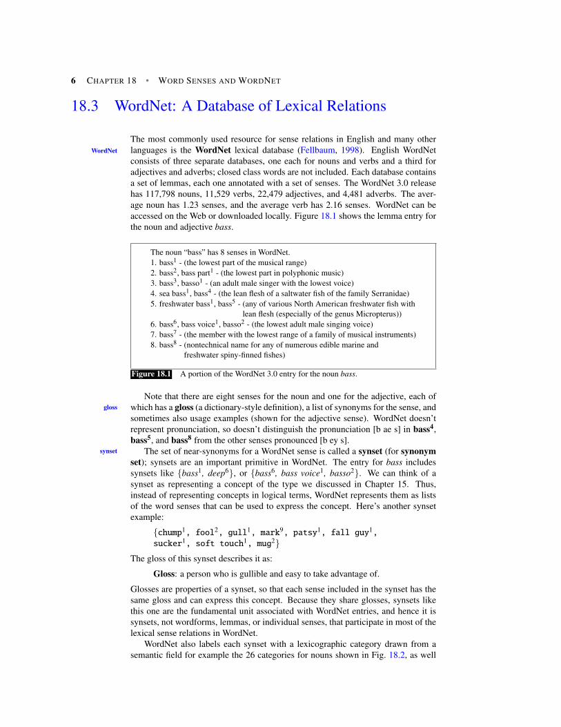
consists of three separate databases, one each for nouns and verbs and a third foradjectives and adverbs; closed class words are not included. Each database containsa set of lemmas, each one annotated with a set of senses. The WordNet 3.0 releasehas 117,798 nouns, 11,529 verbs, 22,479 adjectives, and 4,481 adverbs. The aver-age noun has 1.23 senses, and the average verb has 2.16 senses. WordNet can beaccessed on the Web or downloaded locally. Figure 18.1 shows the lemma entry forthe noun and adjective bass.

The noun “bass” has 8 senses in WordNet.1. bass1 - (the lowest part of the musical range)2. bass2, bass part1 - (the lowest part in polyphonic music)3. bass3, basso1 - (an adult male singer with the lowest voice)4. sea bass1, bass4 - (the lean flesh of a saltwater fish of the family Serranidae)5. freshwater bass1, bass5 - (any of various North American freshwater fish with

lean flesh (especially of the genus Micropterus))6. bass6, bass voice1, basso2 - (the lowest adult male singing voice)7. bass7 - (the member with the lowest range of a family of musical instruments)8. bass8 - (nontechnical name for any of numerous edible marine and

freshwater spiny-finned fishes)

Figure 18.1 A portion of the WordNet 3.0 entry for the noun bass.

Note that there are eight senses for the noun and one for the adjective, each ofwhich has a gloss (a dictionary-style definition), a list of synonyms for the sense, andgloss

sometimes also usage examples (shown for the adjective sense). WordNet doesn’trepresent pronunciation, so doesn’t distinguish the pronunciation [b ae s] in bass4,bass5, and bass8 from the other senses pronounced [b ey s].

The set of near-synonyms for a WordNet sense is called a synset (for synonymsynset

set); synsets are an important primitive in WordNet. The entry for bass includessynsets like {bass1, deep6}, or {bass6, bass voice1, basso2}. We can think of asynset as representing a concept of the type we discussed in Chapter 15. Thus,instead of representing concepts in logical terms, WordNet represents them as listsof the word senses that can be used to express the concept. Here’s another synsetexample:

{chump1, fool2, gull1, mark9, patsy1, fall guy1,

sucker1, soft touch1, mug2}The gloss of this synset describes it as:

Gloss: a person who is gullible and easy to take advantage of.

Glosses are properties of a synset, so that each sense included in the synset has thesame gloss and can express this concept. Because they share glosses, synsets likethis one are the fundamental unit associated with WordNet entries, and hence it issynsets, not wordforms, lemmas, or individual senses, that participate in most of thelexical sense relations in WordNet.

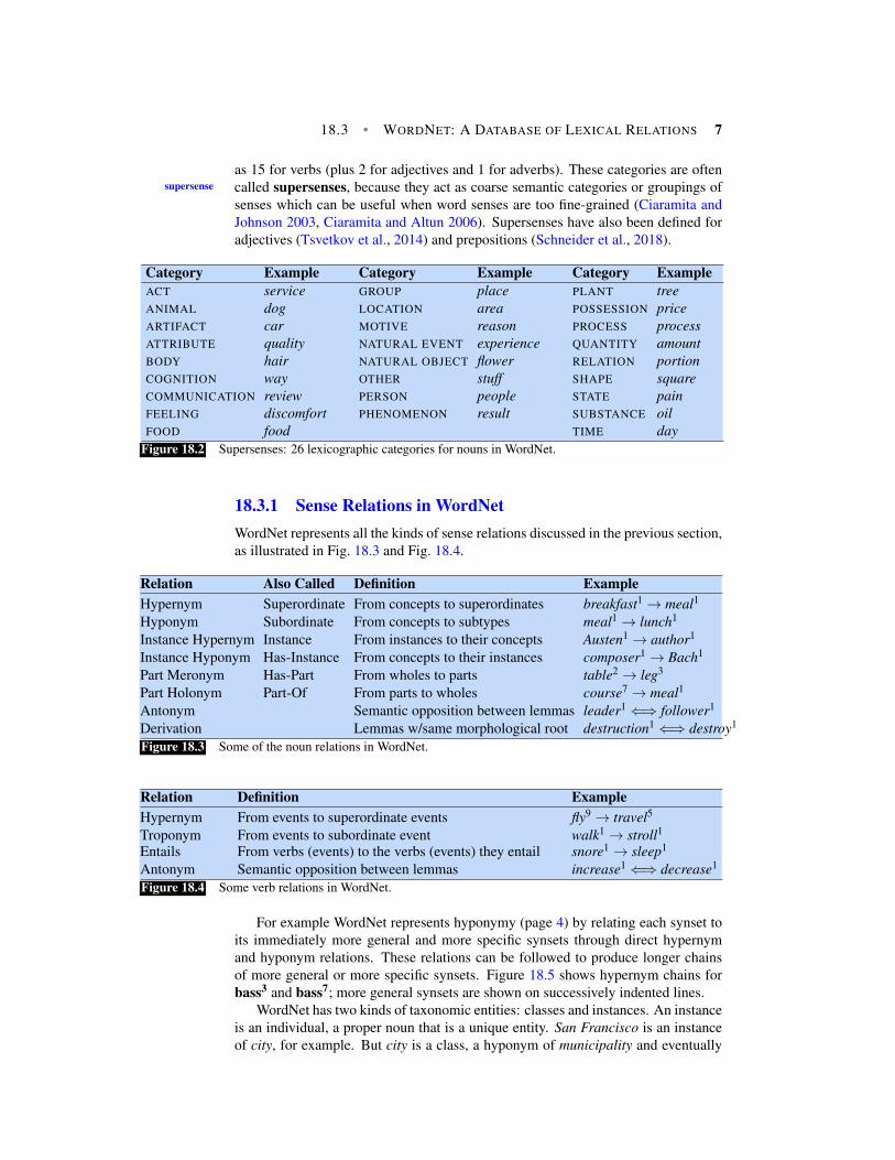
WordNet also labels each synset with a lexicographic category drawn from asemantic field for example the 26 categories for nouns shown in Fig. 18.2, as well

18.3 • WORDNET: A DATABASE OF LEXICAL RELATIONS 7

as 15 for verbs (plus 2 for adjectives and 1 for adverbs). These categories are oftencalled supersenses, because they act as coarse semantic categories or groupings ofsupersense

senses which can be useful when word senses are too fine-grained (Ciaramita andJohnson 2003, Ciaramita and Altun 2006). Supersenses have also been defined foradjectives (Tsvetkov et al., 2014) and prepositions (Schneider et al., 2018).

Category Example Category Example Category ExampleACT service GROUP place PLANT treeANIMAL dog LOCATION area POSSESSION priceARTIFACT car MOTIVE reason PROCESS processATTRIBUTE quality NATURAL EVENT experience QUANTITY amountBODY hair NATURAL OBJECT flower RELATION portionCOGNITION way OTHER stuff SHAPE squareCOMMUNICATION review PERSON people STATE painFEELING discomfort PHENOMENON result SUBSTANCE oilFOOD food TIME day

Figure 18.2 Supersenses: 26 lexicographic categories for nouns in WordNet.

18.3.1 Sense Relations in WordNetWordNet represents all the kinds of sense relations discussed in the previous section,as illustrated in Fig. 18.3 and Fig. 18.4.

Relation Also Called Definition ExampleHypernym Superordinate From concepts to superordinates breakfast1 → meal1

Hyponym Subordinate From concepts to subtypes meal1 → lunch1

Instance Hypernym Instance From instances to their concepts Austen1 → author1

Instance Hyponym Has-Instance From concepts to their instances composer1 → Bach1

Part Meronym Has-Part From wholes to parts table2 → leg3

Part Holonym Part-Of From parts to wholes course7 → meal1

Antonym Semantic opposition between lemmas leader1 ⇐⇒ follower1

Derivation Lemmas w/same morphological root destruction1 ⇐⇒ destroy1

Figure 18.3 Some of the noun relations in WordNet.

Relation Definition ExampleHypernym From events to superordinate events fly9 → travel5

Troponym From events to subordinate event walk1 → stroll1Entails From verbs (events) to the verbs (events) they entail snore1 → sleep1

Antonym Semantic opposition between lemmas increase1 ⇐⇒ decrease1

Figure 18.4 Some verb relations in WordNet.

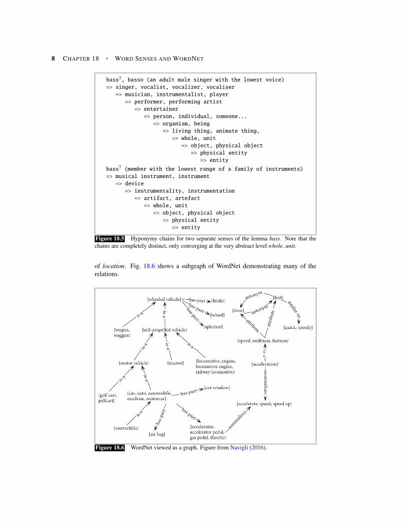
For example WordNet represents hyponymy (page 4) by relating each synset toits immediately more general and more specific synsets through direct hypernymand hyponym relations. These relations can be followed to produce longer chainsof more general or more specific synsets. Figure 18.5 shows hypernym chains forbass3 and bass7; more general synsets are shown on successively indented lines.

WordNet has two kinds of taxonomic entities: classes and instances. An instanceis an individual, a proper noun that is a unique entity. San Francisco is an instanceof city, for example. But city is a class, a hyponym of municipality and eventually

8 CHAPTER 18 • WORD SENSES AND WORDNET

bass3, basso (an adult male singer with the lowest voice)

=> singer, vocalist, vocalizer, vocaliser

=> musician, instrumentalist, player

=> performer, performing artist

=> entertainer

=> person, individual, someone...

=> organism, being

=> living thing, animate thing,

=> whole, unit

=> object, physical object

=> physical entity

=> entity

bass7 (member with the lowest range of a family of instruments)

=> musical instrument, instrument

=> device

=> instrumentality, instrumentation

=> artifact, artefact

=> whole, unit

=> object, physical object

=> physical entity

=> entity

Figure 18.5 Hyponymy chains for two separate senses of the lemma bass. Note that thechains are completely distinct, only converging at the very abstract level whole, unit.

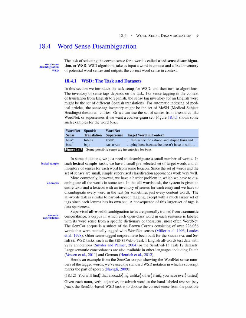
of location. Fig. 18.6 shows a subgraph of WordNet demonstrating many of therelations.

Figure 18.6 WordNet viewed as a graph. Figure from Navigli (2016).

18.4 • WORD SENSE DISAMBIGUATION 9

18.4 Word Sense Disambiguation

The task of selecting the correct sense for a word is called word sense disambigua-tion, or WSD. WSD algorithms take as input a word in context and a fixed inventoryword sense

disambiguationWSD of potential word senses and outputs the correct word sense in context.

18.4.1 WSD: The Task and DatasetsIn this section we introduce the task setup for WSD, and then turn to algorithms.The inventory of sense tags depends on the task. For sense tagging in the contextof translation from English to Spanish, the sense tag inventory for an English wordmight be the set of different Spanish translations. For automatic indexing of med-ical articles, the sense-tag inventory might be the set of MeSH (Medical SubjectHeadings) thesaurus entries. Or we can use the set of senses from a resource likeWordNet, or supersenses if we want a coarser-grain set. Figure 18.4.1 shows somesuch examples for the word bass.

WordNet Spanish WordNetSense Translation Supersense Target Word in Contextbass4 lubina FOOD . . . fish as Pacific salmon and striped bass and. . .bass7 bajo ARTIFACT . . . play bass because he doesn’t have to solo. . .

Figure 18.7 Some possibile sense tag inventories for bass.

In some situations, we just need to disambiguate a small number of words. Insuch lexical sample tasks, we have a small pre-selected set of target words and anlexical sample

inventory of senses for each word from some lexicon. Since the set of words and theset of senses are small, simple supervised classification approaches work very well.

More commonly, however, we have a harder problem in which we have to dis-ambiguate all the words in some text. In this all-words task, the system is given anall-words

entire texts and a lexicon with an inventory of senses for each entry and we have todisambiguate every word in the text (or sometimes just every content word). Theall-words task is similar to part-of-speech tagging, except with a much larger set oftags since each lemma has its own set. A consequence of this larger set of tags isdata sparseness.

Supervised all-word disambiguation tasks are generally trained from a semanticconcordance, a corpus in which each open-class word in each sentence is labeledsemantic

concordancewith its word sense from a specific dictionary or thesaurus, most often WordNet.The SemCor corpus is a subset of the Brown Corpus consisting of over 226,036words that were manually tagged with WordNet senses (Miller et al. 1993, Landeset al. 1998). Other sense-tagged corpora have been built for the SENSEVAL and Se-mEval WSD tasks, such as the SENSEVAL-3 Task 1 English all-words test data with2282 annotations (Snyder and Palmer, 2004) or the SemEval-13 Task 12 datasets.Large semantic concordances are also available in other languages including Dutch(Vossen et al., 2011) and German (Henrich et al., 2012).

Here’s an example from the SemCor corpus showing the WordNet sense num-bers of the tagged words; we’ve used the standard WSD notation in which a subscriptmarks the part of speech (Navigli, 2009):

(18.12) You will find9v that avocado1

n is1v unlike1

j other1j fruit1n you have ever1

r tasted2v

Given each noun, verb, adjective, or adverb word in the hand-labeled test set (sayfruit), the SemCor-based WSD task is to choose the correct sense from the possible

10 CHAPTER 18 • WORD SENSES AND WORDNET

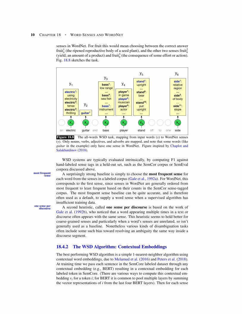
senses in WordNet. For fruit this would mean choosing between the correct answerfruit1n (the ripened reproductive body of a seed plant), and the other two senses fruit2n(yield; an amount of a product) and fruit3n (the consequence of some effort or action).Fig. 18.8 sketches the task.

an electric guitar and bass player stand off to one side

electric1: using

electricityelectric2:

tenseelectric3: thrilling guitar1

bass1: low range

…bass4: sea fish

… bass7:

instrument…

player1: in gameplayer2: musician player3:

actor…

stand1: upright

…stand5:

bear…

stand10: put

upright…

side1: relative region…

side3: of body

… side11: slope…

x1

y1

x2

y2

x3

y3y4

y5 y6

x4 x5 x6

Figure 18.8 The all-words WSD task, mapping from input words (x) to WordNet senses(y). Only nouns, verbs, adjectives, and adverbs are mapped, and note that some words (likeguitar in the example) only have one sense in WordNet. Figure inspired by Chaplot andSalakhutdinov (2018).

WSD systems are typically evaluated intrinsically, by computing F1 againsthand-labeled sense tags in a held-out set, such as the SemCor corpus or SemEvalcorpora discussed above.

A surprisingly strong baseline is simply to choose the most frequent sense formost frequentsense

each word from the senses in a labeled corpus (Gale et al., 1992a). For WordNet, thiscorresponds to the first sense, since senses in WordNet are generally ordered frommost frequent to least frequent based on their counts in the SemCor sense-taggedcorpus. The most frequent sense baseline can be quite accurate, and is thereforeoften used as a default, to supply a word sense when a supervised algorithm hasinsufficient training data.

A second heuristic, called one sense per discourse is based on the work ofone sense perdiscourse

Gale et al. (1992b), who noticed that a word appearing multiple times in a text ordiscourse often appears with the same sense. This heuristic seems to hold better forcoarse-grained senses and particularly when a word’s senses are unrelated, so isn’tgenerally used as a baseline. Nonetheless various kinds of disambiguation tasksoften include some such bias toward resolving an ambiguity the same way inside adiscourse segment.

18.4.2 The WSD Algorithm: Contextual EmbeddingsThe best performing WSD algorithm is a simple 1-nearest-neighbor algorithm usingcontextual word embeddings, due to Melamud et al. (2016) and Peters et al. (2018).At training time we pass each sentence in the SemCore labeled dataset through anycontextual embedding (e.g., BERT) resulting in a contextual embedding for eachlabeled token in SemCore. (There are various ways to compute this contextual em-bedding vi for a token i; for BERT it is common to pool multiple layers by summingthe vector representations of i from the last four BERT layers). Then for each sense

18.4 • WORD SENSE DISAMBIGUATION 11

s of any word in the corpus, for each of the n tokens of that sense, we average theirn contextual representations vi to produce a contextual sense embedding vs for s:

vs =1n

∑i

vi ∀vi ∈ tokens(s) (18.13)

At test time, given a token of a target word t in context, we compute its contextualembedding t and choose its nearest neighbor sense from the training set, i.e., thesense whose sense embedding has the highest cosine with t:

sense(t) = argmaxs∈senses(t)

cosine(t,vs) (18.14)

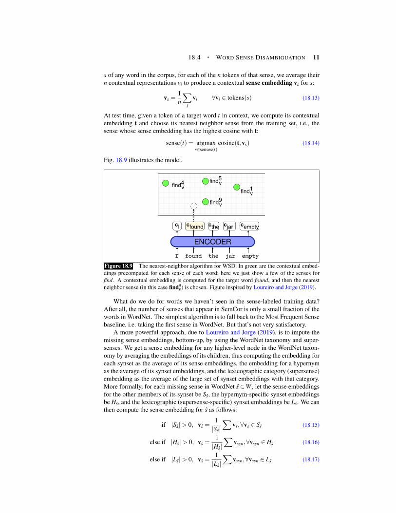
Fig. 18.9 illustrates the model.

I found the jar empty

cI cfound

find1v

cthe cjar cempty

find9v

find5vfind4v

ENCODER

Figure 18.9 The nearest-neighbor algorithm for WSD. In green are the contextual embed-dings precomputed for each sense of each word; here we just show a few of the senses forfind. A contextual embedding is computed for the target word found, and then the nearestneighbor sense (in this case find9

v) is chosen. Figure inspired by Loureiro and Jorge (2019).

What do we do for words we haven’t seen in the sense-labeled training data?After all, the number of senses that appear in SemCor is only a small fraction of thewords in WordNet. The simplest algorithm is to fall back to the Most Frequent Sensebaseline, i.e. taking the first sense in WordNet. But that’s not very satisfactory.

A more powerful approach, due to Loureiro and Jorge (2019), is to impute themissing sense embeddings, bottom-up, by using the WordNet taxonomy and super-senses. We get a sense embedding for any higher-level node in the WordNet taxon-omy by averaging the embeddings of its children, thus computing the embedding foreach synset as the average of its sense embeddings, the embedding for a hypernymas the average of its synset embeddings, and the lexicographic category (supersense)embedding as the average of the large set of synset embeddings with that category.More formally, for each missing sense in WordNet s ∈W , let the sense embeddingsfor the other members of its synset be Ss, the hypernym-specific synset embeddingsbe Hs, and the lexicographic (supersense-specific) synset embeddings be Ls. We canthen compute the sense embedding for s as follows:

if |Ss|> 0, vs =1|Ss|

∑vs,∀vs ∈ Ss (18.15)

else if |Hs|> 0, vs =1|Hs|

∑vsyn,∀vsyn ∈ Hs (18.16)

else if |Ls|> 0, vs =1|Ls|

∑vsyn,∀vsyn ∈ Ls (18.17)

12 CHAPTER 18 • WORD SENSES AND WORDNET

Since all of the supersenses have some labeled data in SemCor, the algorithm isguaranteed to have some representation for all possible senses by the time the al-gorithm backs off to the most general (supersense) information, although of coursewith a very coarse model.

18.5 Alternate WSD algorithms and Tasks

18.5.1 Feature-Based WSDFeature-based algorithms for WSD are extremely simple and function almost aswell as contextual language model algorithms. The best performing IMS algorithm(Zhong and Ng, 2010), augmented by embeddings (Iacobacci et al. 2016, Raganatoet al. 2017b), uses an SVM classifier to choose the sense for each input word withthe following simple features of the surrounding words:

• part-of-speech tags (for a window of 3 words on each side, stopping at sen-tence boundaries)

• collocation features of words or n-grams of lengths 1, 2, 3 at a particularcollocation

location in a window of 3 words on each side (i.e., exactly one word to theright, or the two words starting 3 words to the left, and so on).

• weighted average of embeddings (of all words in a window of 10 words oneach side, weighted exponentially by distance)

Consider the ambiguous word bass in the following WSJ sentence:

(18.18) An electric guitar and bass player stand off to one side,

If we used a small 2-word window, a standard feature vector might include parts-of-speech, unigram and bigram collocation features, and a weighted sum g of embed-dings, that is:

[wi−2,POSi−2,wi−1,POSi−1,wi+1,POSi+1,wi+2,POSi+2,wi−1i−2,

wi+2i+1,g(E(wi−2),E(wi−1),E(wi+1),E(wi+2)] (18.19)

would yield the following vector:

[guitar, NN, and, CC, player, NN, stand, VB, guitar and,

player stand, g(E(guitar),E(and),E(player),E(stand))]

18.5.2 The Lesk Algorithm as WSD BaselineGenerating sense labeled corpora like SemCor is quite difficult and expensive. Analternative class of WSD algorithms, knowledge-based algorithms, rely solely onknowledge-

basedWordNet or other such resources and don’t require labeled data. While supervisedalgorithms generally work better, knowledge-based methods can be used in lan-guages or domains where thesauruses or dictionaries but not sense labeled corporaare available.

The Lesk algorithm is the oldest and most powerful knowledge-based WSDLesk algorithm

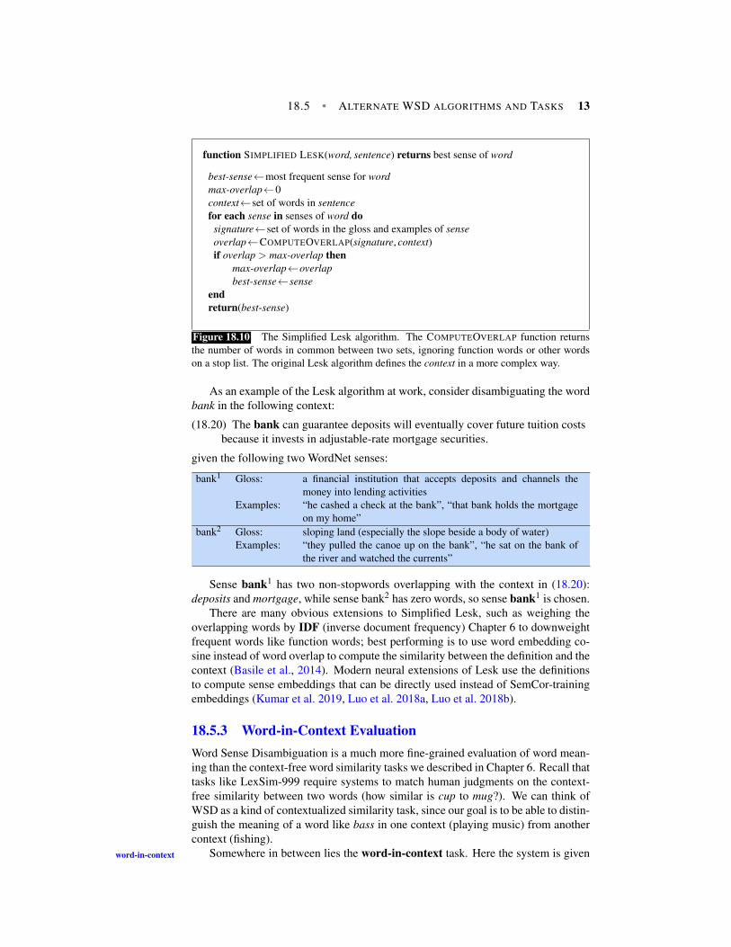
method, and is a useful baseline. Lesk is really a family of algorithms that choosethe sense whose dictionary gloss or definition shares the most words with the targetword’s neighborhood. Figure 18.10 shows the simplest version of the algorithm,often called the Simplified Lesk algorithm (Kilgarriff and Rosenzweig, 2000).Simplified Lesk

18.5 • ALTERNATE WSD ALGORITHMS AND TASKS 13

function SIMPLIFIED LESK(word, sentence) returns best sense of word

best-sense←most frequent sense for wordmax-overlap←0context←set of words in sentencefor each sense in senses of word dosignature←set of words in the gloss and examples of senseoverlap←COMPUTEOVERLAP(signature, context)if overlap > max-overlap then

max-overlap←overlapbest-sense←sense

endreturn(best-sense)

Figure 18.10 The Simplified Lesk algorithm. The COMPUTEOVERLAP function returnsthe number of words in common between two sets, ignoring function words or other wordson a stop list. The original Lesk algorithm defines the context in a more complex way.

As an example of the Lesk algorithm at work, consider disambiguating the wordbank in the following context:

(18.20) The bank can guarantee deposits will eventually cover future tuition costsbecause it invests in adjustable-rate mortgage securities.

given the following two WordNet senses:

bank1 Gloss: a financial institution that accepts deposits and channels themoney into lending activities

Examples: “he cashed a check at the bank”, “that bank holds the mortgageon my home”

bank2 Gloss: sloping land (especially the slope beside a body of water)Examples: “they pulled the canoe up on the bank”, “he sat on the bank of

the river and watched the currents”

Sense bank1 has two non-stopwords overlapping with the context in (18.20):deposits and mortgage, while sense bank2 has zero words, so sense bank1 is chosen.

There are many obvious extensions to Simplified Lesk, such as weighing theoverlapping words by IDF (inverse document frequency) Chapter 6 to downweightfrequent words like function words; best performing is to use word embedding co-sine instead of word overlap to compute the similarity between the definition and thecontext (Basile et al., 2014). Modern neural extensions of Lesk use the definitionsto compute sense embeddings that can be directly used instead of SemCor-trainingembeddings (Kumar et al. 2019, Luo et al. 2018a, Luo et al. 2018b).

18.5.3 Word-in-Context EvaluationWord Sense Disambiguation is a much more fine-grained evaluation of word mean-ing than the context-free word similarity tasks we described in Chapter 6. Recall thattasks like LexSim-999 require systems to match human judgments on the context-free similarity between two words (how similar is cup to mug?). We can think ofWSD as a kind of contextualized similarity task, since our goal is to be able to distin-guish the meaning of a word like bass in one context (playing music) from anothercontext (fishing).

Somewhere in between lies the word-in-context task. Here the system is givenword-in-context

14 CHAPTER 18 • WORD SENSES AND WORDNET

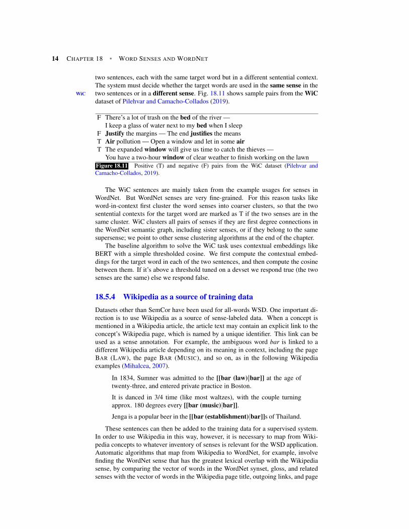
two sentences, each with the same target word but in a different sentential context.The system must decide whether the target words are used in the same sense in thetwo sentences or in a different sense. Fig. 18.11 shows sample pairs from the WiCWiC

dataset of Pilehvar and Camacho-Collados (2019).

F There’s a lot of trash on the bed of the river —I keep a glass of water next to my bed when I sleep

F Justify the margins — The end justifies the meansT Air pollution — Open a window and let in some airT The expanded window will give us time to catch the thieves —

You have a two-hour window of clear weather to finish working on the lawnFigure 18.11 Positive (T) and negative (F) pairs from the WiC dataset (Pilehvar andCamacho-Collados, 2019).

The WiC sentences are mainly taken from the example usages for senses inWordNet. But WordNet senses are very fine-grained. For this reason tasks likeword-in-context first cluster the word senses into coarser clusters, so that the twosentential contexts for the target word are marked as T if the two senses are in thesame cluster. WiC clusters all pairs of senses if they are first degree connections inthe WordNet semantic graph, including sister senses, or if they belong to the samesupersense; we point to other sense clustering algorithms at the end of the chapter.

The baseline algorithm to solve the WiC task uses contextual embeddings likeBERT with a simple thresholded cosine. We first compute the contextual embed-dings for the target word in each of the two sentences, and then compute the cosinebetween them. If it’s above a threshold tuned on a devset we respond true (the twosenses are the same) else we respond false.

18.5.4 Wikipedia as a source of training dataDatasets other than SemCor have been used for all-words WSD. One important di-rection is to use Wikipedia as a source of sense-labeled data. When a concept ismentioned in a Wikipedia article, the article text may contain an explicit link to theconcept’s Wikipedia page, which is named by a unique identifier. This link can beused as a sense annotation. For example, the ambiguous word bar is linked to adifferent Wikipedia article depending on its meaning in context, including the pageBAR (LAW), the page BAR (MUSIC), and so on, as in the following Wikipediaexamples (Mihalcea, 2007).

In 1834, Sumner was admitted to the [[bar (law)|bar]] at the age oftwenty-three, and entered private practice in Boston.

It is danced in 3/4 time (like most waltzes), with the couple turningapprox. 180 degrees every [[bar (music)|bar]].

Jenga is a popular beer in the [[bar (establishment)|bar]]s of Thailand.

These sentences can then be added to the training data for a supervised system.In order to use Wikipedia in this way, however, it is necessary to map from Wiki-pedia concepts to whatever inventory of senses is relevant for the WSD application.Automatic algorithms that map from Wikipedia to WordNet, for example, involvefinding the WordNet sense that has the greatest lexical overlap with the Wikipediasense, by comparing the vector of words in the WordNet synset, gloss, and relatedsenses with the vector of words in the Wikipedia page title, outgoing links, and page

18.6 • USING THESAURUSES TO IMPROVE EMBEDDINGS 15

category (Ponzetto and Navigli, 2010). The resulting mapping has been used tocreate BabelNet, a large sense-annotated resource (Navigli and Ponzetto, 2012).

18.6 Using Thesauruses to Improve Embeddings

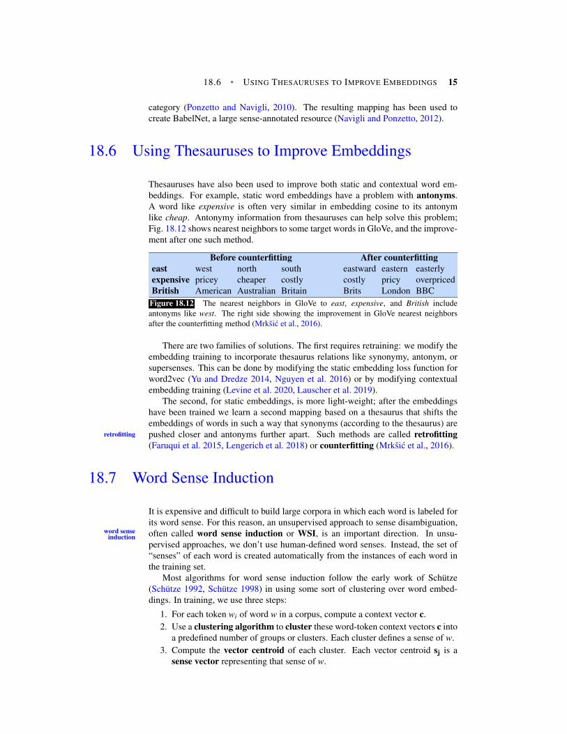
Thesauruses have also been used to improve both static and contextual word em-beddings. For example, static word embeddings have a problem with antonyms.A word like expensive is often very similar in embedding cosine to its antonymlike cheap. Antonymy information from thesauruses can help solve this problem;Fig. 18.12 shows nearest neighbors to some target words in GloVe, and the improve-ment after one such method.

Before counterfitting After counterfittingeast west north south eastward eastern easterlyexpensive pricey cheaper costly costly pricy overpricedBritish American Australian Britain Brits London BBC

Figure 18.12 The nearest neighbors in GloVe to east, expensive, and British includeantonyms like west. The right side showing the improvement in GloVe nearest neighborsafter the counterfitting method (Mrksic et al., 2016).

There are two families of solutions. The first requires retraining: we modify theembedding training to incorporate thesaurus relations like synonymy, antonym, orsupersenses. This can be done by modifying the static embedding loss function forword2vec (Yu and Dredze 2014, Nguyen et al. 2016) or by modifying contextualembedding training (Levine et al. 2020, Lauscher et al. 2019).

The second, for static embeddings, is more light-weight; after the embeddingshave been trained we learn a second mapping based on a thesaurus that shifts theembeddings of words in such a way that synonyms (according to the thesaurus) arepushed closer and antonyms further apart. Such methods are called retrofittingretrofitting

(Faruqui et al. 2015, Lengerich et al. 2018) or counterfitting (Mrksic et al., 2016).

18.7 Word Sense Induction

It is expensive and difficult to build large corpora in which each word is labeled forits word sense. For this reason, an unsupervised approach to sense disambiguation,often called word sense induction or WSI, is an important direction. In unsu-word sense

inductionpervised approaches, we don’t use human-defined word senses. Instead, the set of“senses” of each word is created automatically from the instances of each word inthe training set.

Most algorithms for word sense induction follow the early work of Schutze(Schutze 1992, Schutze 1998) in using some sort of clustering over word embed-dings. In training, we use three steps:

1. For each token wi of word w in a corpus, compute a context vector c.2. Use a clustering algorithm to cluster these word-token context vectors c into

a predefined number of groups or clusters. Each cluster defines a sense of w.3. Compute the vector centroid of each cluster. Each vector centroid sj is a

sense vector representing that sense of w.

16 CHAPTER 18 • WORD SENSES AND WORDNET

Since this is an unsupervised algorithm, we don’t have names for each of these“senses” of w; we just refer to the jth sense of w.

To disambiguate a particular token t of w we again have three steps:

1. Compute a context vector c for t.2. Retrieve all sense vectors s j for w.3. Assign t to the sense represented by the sense vector s j that is closest to t.

All we need is a clustering algorithm and a distance metric between vectors.Clustering is a well-studied problem with a wide number of standard algorithms thatcan be applied to inputs structured as vectors of numerical values (Duda and Hart,1973). A frequently used technique in language applications is known as agglom-erative clustering. In this technique, each of the N training instances is initiallyagglomerative

clusteringassigned to its own cluster. New clusters are then formed in a bottom-up fashion bythe successive merging of the two clusters that are most similar. This process con-tinues until either a specified number of clusters is reached, or some global goodnessmeasure among the clusters is achieved. In cases in which the number of traininginstances makes this method too expensive, random sampling can be used on theoriginal training set to achieve similar results.

How can we evaluate unsupervised sense disambiguation approaches? As usual,the best way is to do extrinsic evaluation embedded in some end-to-end system; oneexample used in a SemEval bakeoff is to improve search result clustering and di-versification (Navigli and Vannella, 2013). Intrinsic evaluation requires a way tomap the automatically derived sense classes into a hand-labeled gold-standard set sothat we can compare a hand-labeled test set with a set labeled by our unsupervisedclassifier. Various such metrics have been tested, for example in the SemEval tasks(Manandhar et al. 2010, Navigli and Vannella 2013, Jurgens and Klapaftis 2013),including cluster overlap metrics, or methods that map each sense cluster to a pre-defined sense by choosing the sense that (in some training set) has the most overlapwith the cluster. However it is fair to say that no evaluation metric for this task hasyet become standard.

18.8 Summary

This chapter has covered a wide range of issues concerning the meanings associatedwith lexical items. The following are among the highlights:

• A word sense is the locus of word meaning; definitions and meaning relationsare defined at the level of the word sense rather than wordforms.

• Many words are polysemous, having many senses.• Relations between senses include synonymy, antonymy, meronymy, and

taxonomic relations hyponymy and hypernymy.• WordNet is a large database of lexical relations for English, and WordNets

exist for a variety of languages.• Word-sense disambiguation (WSD) is the task of determining the correct

sense of a word in context. Supervised approaches make use of a corpusof sentences in which individual words (lexical sample task) or all words(all-words task) are hand-labeled with senses from a resource like WordNet.SemCor is the largest corpus with WordNet-labeled senses.

BIBLIOGRAPHICAL AND HISTORICAL NOTES 17

• The standard supervised algorithm for WSD is nearest neighbors with contex-tual embeddings.

• Feature-based algorithms using parts of speech and embeddings of words inthe context of the target word also work well.

• An important baseline for WSD is the most frequent sense, equivalent, inWordNet, to take the first sense.

• Another baseline is a knowledge-based WSD algorithm called the Lesk al-gorithm which chooses the sense whose dictionary definition shares the mostwords with the target word’s neighborhood.

• Word sense induction is the task of learning word senses unsupervised.

Bibliographical and Historical NotesWord sense disambiguation traces its roots to some of the earliest applications ofdigital computers. The insight that underlies modern algorithms for word sense dis-ambiguation was first articulated by Weaver (1949/1955) in the context of machinetranslation:

If one examines the words in a book, one at a time as through an opaquemask with a hole in it one word wide, then it is obviously impossibleto determine, one at a time, the meaning of the words. [. . . ] But ifone lengthens the slit in the opaque mask, until one can see not onlythe central word in question but also say N words on either side, thenif N is large enough one can unambiguously decide the meaning of thecentral word. [. . . ] The practical question is : “What minimum value ofN will, at least in a tolerable fraction of cases, lead to the correct choiceof meaning for the central word?”

Other notions first proposed in this early period include the use of a thesaurus for dis-ambiguation (Masterman, 1957), supervised training of Bayesian models for disam-biguation (Madhu and Lytel, 1965), and the use of clustering in word sense analysis(Sparck Jones, 1986).

Much disambiguation work was conducted within the context of early AI-orientednatural language processing systems. Quillian (1968) and Quillian (1969) proposeda graph-based approach to language processing, in which the definition of a wordwas represented by a network of word nodes connected by syntactic and semanticrelations, and sense disambiguation by finding the shortest path between senses inthe graph. Simmons (1973) is another influential early semantic network approach.Wilks proposed one of the earliest non-discrete models with his Preference Seman-tics (Wilks 1975c, Wilks 1975b, Wilks 1975a), and Small and Rieger (1982) andRiesbeck (1975) proposed understanding systems based on modeling rich procedu-ral information for each word. Hirst’s ABSITY system (Hirst and Charniak 1982,Hirst 1987, Hirst 1988), which used a technique called marker passing based on se-mantic networks, represents the most advanced system of this type. As with theselargely symbolic approaches, early neural network (at the time called ‘connection-ist’) approaches to word sense disambiguation relied on small lexicons with hand-coded representations (Cottrell 1985, Kawamoto 1988).

The earliest implementation of a robust empirical approach to sense disambigua-tion is due to Kelly and Stone (1975), who directed a team that hand-crafted a set

18 CHAPTER 18 • WORD SENSES AND WORDNET

of disambiguation rules for 1790 ambiguous English words. Lesk (1986) was thefirst to use a machine-readable dictionary for word sense disambiguation. Fellbaum(1998) collects early work on WordNet. Early work using dictionaries as lexicalresources include Amsler’s 1981 use of the Merriam Webster dictionary and Long-man’s Dictionary of Contemporary English (Boguraev and Briscoe, 1989).

Supervised approaches to disambiguation began with the use of decision treesby Black (1988). In addition to the IMS and contextual-embedding based methodsfor supervised WSD, recent supervised algorithms includes encoder-decoder models(Raganato et al., 2017a).

The need for large amounts of annotated text in supervised methods led earlyon to investigations into the use of bootstrapping methods (Hearst 1991, Yarowsky1995). For example the semi-supervised algorithm of Diab and Resnik (2002) isbased on aligned parallel corpora in two languages. For example, the fact that theFrench word catastrophe might be translated as English disaster in one instanceand tragedy in another instance can be used to disambiguate the senses of the twoEnglish words (i.e., to choose senses of disaster and tragedy that are similar).

The earliest use of clustering in the study of word senses was by Sparck Jones(1986); Pedersen and Bruce (1997), Schutze (1997), and Schutze (1998) applied dis-tributional methods. Clustering word senses into coarse senses has also been usedcoarse senses

to address the problem of dictionary senses being too fine-grained (Section 18.5.3)(Dolan 1994, Chen and Chang 1998, Mihalcea and Moldovan 2001, Agirre andde Lacalle 2003, Palmer et al. 2004, Navigli 2006, Snow et al. 2007, Pilehvar et al.2013). Corpora with clustered word senses for training supervised clustering algo-rithms include Palmer et al. (2006) and OntoNotes (Hovy et al., 2006).OntoNotes

See Pustejovsky (1995), Pustejovsky and Boguraev (1996), Martin (1986), andCopestake and Briscoe (1995), inter alia, for computational approaches to the rep-resentation of polysemy. Pustejovsky’s theory of the generative lexicon, and ingenerative

lexiconparticular his theory of the qualia structure of words, is a way of accounting for thequalia

structuredynamic systematic polysemy of words in context.

Historical overviews of WSD include Agirre and Edmonds (2006) and Navigli(2009).

Exercises18.1 Collect a small corpus of example sentences of varying lengths from any

newspaper or magazine. Using WordNet or any standard dictionary, deter-mine how many senses there are for each of the open-class words in each sen-tence. How many distinct combinations of senses are there for each sentence?How does this number seem to vary with sentence length?

18.2 Using WordNet or a standard reference dictionary, tag each open-class wordin your corpus with its correct tag. Was choosing the correct sense always astraightforward task? Report on any difficulties you encountered.

18.3 Using your favorite dictionary, simulate the original Lesk word overlap dis-ambiguation algorithm described on page 13 on the phrase Time flies like anarrow. Assume that the words are to be disambiguated one at a time, fromleft to right, and that the results from earlier decisions are used later in theprocess.

EXERCISES 19

18.4 Build an implementation of your solution to the previous exercise. UsingWordNet, implement the original Lesk word overlap disambiguation algo-rithm described on page 13 on the phrase Time flies like an arrow.

20 Chapter 18 • Word Senses and WordNet

Agirre, E. and O. L. de Lacalle. 2003. Clustering WordNetword senses. RANLP 2003.

Agirre, E. and P. Edmonds, editors. 2006. Word Sense Dis-ambiguation: Algorithms and Applications. Kluwer.

Amsler, R. A. 1981. A taxonomy for English nouns andverbs. ACL.

Basile, P., A. Caputo, and G. Semeraro. 2014. An enhancedLesk word sense disambiguation algorithm through a dis-tributional semantic model. COLING.

Black, E. 1988. An experiment in computational discrimi-nation of English word senses. IBM Journal of Researchand Development, 32(2):185–194.

Boguraev, B. K. and T. Briscoe, editors. 1989. Computa-tional Lexicography for Natural Language Processing.Longman.

Chaplot, D. S. and R. Salakhutdinov. 2018. Knowledge-based word sense disambiguation using topic models.AAAI.

Chen, J. N. and J. S. Chang. 1998. Topical clustering ofMRD senses based on information retrieval techniques.Computational Linguistics, 24(1):61–96.

Ciaramita, M. and Y. Altun. 2006. Broad-coverage sensedisambiguation and information extraction with a super-sense sequence tagger. EMNLP.

Ciaramita, M. and M. Johnson. 2003. Supersense tagging ofunknown nouns in WordNet. EMNLP-2003.

Copestake, A. and T. Briscoe. 1995. Semi-productivepolysemy and sense extension. Journal of Semantics,12(1):15–68.

Cottrell, G. W. 1985. A Connectionist Approach to WordSense Disambiguation. Ph.D. thesis, University ofRochester, Rochester, NY. Revised version published byPitman, 1989.

Diab, M. and P. Resnik. 2002. An unsupervised method forword sense tagging using parallel corpora. ACL.

Dolan, B. 1994. Word sense ambiguation: Clustering relatedsenses. COLING.

Duda, R. O. and P. E. Hart. 1973. Pattern Classification andScene Analysis. John Wiley and Sons.

Faruqui, M., J. Dodge, S. K. Jauhar, C. Dyer, E. Hovy, andN. A. Smith. 2015. Retrofitting word vectors to semanticlexicons. NAACL HLT.

Fellbaum, C., editor. 1998. WordNet: An Electronic LexicalDatabase. MIT Press.

Gale, W. A., K. W. Church, and D. Yarowsky. 1992a. Es-timating upper and lower bounds on the performance ofword-sense disambiguation programs. ACL.

Gale, W. A., K. W. Church, and D. Yarowsky. 1992b. Onesense per discourse. HLT.

Haber, J. and M. Poesio. 2020. Assessing polyseme sensesimilarity through co-predication acceptability and con-textualised embedding distance. *SEM.

Hearst, M. A. 1991. Noun homograph disambiguation. Pro-ceedings of the 7th Conference of the University of Wa-terloo Centre for the New OED and Text Research.

Henrich, V., E. Hinrichs, and T. Vodolazova. 2012. We-bCAGe – a web-harvested corpus annotated with Ger-maNet senses. EACL.

Hirst, G. 1987. Semantic Interpretation and the Resolutionof Ambiguity. Cambridge University Press.

Hirst, G. 1988. Resolving lexical ambiguity computationallywith spreading activation and polaroid words. In S. L.Small, G. W. Cottrell, and M. K. Tanenhaus, editors, Lex-ical Ambiguity Resolution, pages 73–108. Morgan Kauf-mann.

Hirst, G. and E. Charniak. 1982. Word sense and case slotdisambiguation. AAAI.

Hovy, E. H., M. P. Marcus, M. Palmer, L. A. Ramshaw,and R. Weischedel. 2006. OntoNotes: The 90% solution.HLT-NAACL.

Iacobacci, I., M. T. Pilehvar, and R. Navigli. 2016. Em-beddings for word sense disambiguation: An evaluationstudy. ACL.

Jurgens, D. and I. P. Klapaftis. 2013. SemEval-2013 task 13:Word sense induction for graded and non-graded senses.*SEM.

Kawamoto, A. H. 1988. Distributed representations of am-biguous words and their resolution in connectionist net-works. In S. L. Small, G. W. Cottrell, and M. Tanen-haus, editors, Lexical Ambiguity Resolution, pages 195–228. Morgan Kaufman.

Kelly, E. F. and P. J. Stone. 1975. Computer Recognition ofEnglish Word Senses. North-Holland.

Kilgarriff, A. and J. Rosenzweig. 2000. Framework and re-sults for English SENSEVAL. Computers and the Hu-manities, 34:15–48.

Kumar, S., S. Jat, K. Saxena, and P. Talukdar. 2019. Zero-shot word sense disambiguation using sense definitionembeddings. ACL.

Landes, S., C. Leacock, and R. I. Tengi. 1998. Buildingsemantic concordances. In C. Fellbaum, editor, Word-Net: An Electronic Lexical Database, pages 199–216.MIT Press.

Lauscher, A., I. Vulic, E. M. Ponti, A. Korhonen, andG. Glavas. 2019. Informing unsupervised pretrainingwith external linguistic knowledge. ArXiv preprintarXiv:1909.02339.

Lengerich, B., A. Maas, and C. Potts. 2018. Retrofitting dis-tributional embeddings to knowledge graphs with func-tional relations. COLING.

Lesk, M. E. 1986. Automatic sense disambiguation usingmachine readable dictionaries: How to tell a pine conefrom an ice cream cone. Proceedings of the 5th Interna-tional Conference on Systems Documentation.

Levine, Y., B. Lenz, O. Dagan, O. Ram, D. Pad-nos, O. Sharir, S. Shalev-Shwartz, A. Shashua, andY. Shoham. 2020. SenseBERT: Driving some sense intoBERT. ACL.

Loureiro, D. and A. Jorge. 2019. Language modelling makessense: Propagating representations through WordNet forfull-coverage word sense disambiguation. ACL.

Luo, F., T. Liu, Z. He, Q. Xia, Z. Sui, and B. Chang. 2018a.Leveraging gloss knowledge in neural word sense disam-biguation by hierarchical co-attention. EMNLP.

Luo, F., T. Liu, Q. Xia, B. Chang, and Z. Sui. 2018b. Incor-porating glosses into neural word sense disambiguation.ACL.

Exercises 21

Madhu, S. and D. Lytel. 1965. A figure of merit technique forthe resolution of non-grammatical ambiguity. MechanicalTranslation, 8(2):9–13.

Manandhar, S., I. P. Klapaftis, D. Dligach, and S. Pradhan.2010. SemEval-2010 task 14: Word sense induction &disambiguation. SemEval.

Martin, J. H. 1986. The acquisition of polysemy. ICML.Masterman, M. 1957. The thesaurus in syntax and semantics.

Mechanical Translation, 4(1):1–2.Melamud, O., J. Goldberger, and I. Dagan. 2016. con-

text2vec: Learning generic context embedding with bidi-rectional LSTM. CoNLL.

Mihalcea, R. 2007. Using Wikipedia for automatic wordsense disambiguation. NAACL-HLT.

Mihalcea, R. and D. Moldovan. 2001. Automatic genera-tion of a coarse grained WordNet. NAACL Workshop onWordNet and Other Lexical Resources.

Miller, G. A., C. Leacock, R. I. Tengi, and R. T. Bunker.1993. A semantic concordance. HLT.

Morris, W., editor. 1985. American Heritage Dictionary, 2ndcollege edition edition. Houghton Mifflin.

Mrksic, N., D. O. Seaghdha, B. Thomson, M. Gasic, L. M.Rojas-Barahona, P.-H. Su, D. Vandyke, T.-H. Wen, andS. Young. 2016. Counter-fitting word vectors to linguis-tic constraints. NAACL HLT.

Navigli, R. 2006. Meaningful clustering of senses helpsboost word sense disambiguation performance. COL-ING/ACL.

Navigli, R. 2009. Word sense disambiguation: A survey.ACM Computing Surveys, 41(2).

Navigli, R. 2016. Chapter 20. ontologies. In R. Mitkov, ed-itor, The Oxford handbook of computational linguistics.Oxford University Press.

Navigli, R. and S. P. Ponzetto. 2012. BabelNet: The auto-matic construction, evaluation and application of a wide-coverage multilingual semantic network. Artificial Intel-ligence, 193:217–250.

Navigli, R. and D. Vannella. 2013. SemEval-2013 task 11:Word sense induction and disambiguation within an end-user application. *SEM.

Nguyen, K. A., S. Schulte im Walde, and N. T. Vu. 2016.Integrating distributional lexical contrast into word em-beddings for antonym-synonym distinction. ACL.

Palmer, M., O. Babko-Malaya, and H. T. Dang. 2004. Dif-ferent sense granularities for different applications. HLT-NAACL Workshop on Scalable Natural Language Under-standing.

Palmer, M., H. T. Dang, and C. Fellbaum. 2006. Makingfine-grained and coarse-grained sense distinctions, bothmanually and automatically. Natural Language Engineer-ing, 13(2):137–163.

Pedersen, T. and R. Bruce. 1997. Distinguishing word sensesin untagged text. EMNLP.

Peters, M., M. Neumann, M. Iyyer, M. Gardner, C. Clark,K. Lee, and L. Zettlemoyer. 2018. Deep contextualizedword representations. NAACL HLT.

Pilehvar, M. T. and J. Camacho-Collados. 2019. WiC: theword-in-context dataset for evaluating context-sensitivemeaning representations. NAACL HLT.

Pilehvar, M. T., D. Jurgens, and R. Navigli. 2013. Align,disambiguate and walk: A unified approach for measur-ing semantic similarity. ACL.

Ponzetto, S. P. and R. Navigli. 2010. Knowledge-rich wordsense disambiguation rivaling supervised systems. ACL.

Pu, X., N. Pappas, J. Henderson, and A. Popescu-Belis.2018. Integrating weakly supervised word sense disam-biguation into neural machine translation. TACL, 6:635–649.

Pustejovsky, J. 1995. The Generative Lexicon. MIT Press.

Pustejovsky, J. and B. K. Boguraev, editors. 1996. LexicalSemantics: The Problem of Polysemy. Oxford UniversityPress.

Quillian, M. R. 1968. Semantic memory. In M. Minsky,editor, Semantic Information Processing, pages 227–270.MIT Press.

Quillian, M. R. 1969. The teachable language compre-hender: A simulation program and theory of language.CACM, 12(8):459–476.

Raganato, A., C. D. Bovi, and R. Navigli. 2017a. Neural se-quence learning models for word sense disambiguation.EMNLP.

Raganato, A., J. Camacho-Collados, and R. Navigli. 2017b.Word sense disambiguation: A unified evaluation frame-work and empirical comparison. EACL.

Riesbeck, C. K. 1975. Conceptual analysis. In R. C. Schank,editor, Conceptual Information Processing, pages 83–156. American Elsevier, New York.

Schneider, N., J. D. Hwang, V. Srikumar, J. Prange, A. Blod-gett, S. R. Moeller, A. Stern, A. Bitan, and O. Abend.2018. Comprehensive supersense disambiguation of En-glish prepositions and possessives. ACL.

Schutze, H. 1992. Dimensions of meaning. Proceedings ofSupercomputing ’92. IEEE Press.

Schutze, H. 1997. Ambiguity Resolution in Language Learn-ing: Computational and Cognitive Models. CSLI Publi-cations, Stanford, CA.

Schutze, H. 1998. Automatic word sense discrimination.Computational Linguistics, 24(1):97–124.

Simmons, R. F. 1973. Semantic networks: Their compu-tation and use for understanding English sentences. InR. C. Schank and K. M. Colby, editors, Computer Modelsof Thought and Language, pages 61–113. W.H. Freemanand Co.

Small, S. L. and C. Rieger. 1982. Parsing and comprehend-ing with Word Experts. In W. G. Lehnert and M. H.Ringle, editors, Strategies for Natural Language Process-ing, pages 89–147. Lawrence Erlbaum.

Snow, R., S. Prakash, D. Jurafsky, and A. Y. Ng. 2007.Learning to merge word senses. EMNLP/CoNLL.

Snyder, B. and M. Palmer. 2004. The English all-words task.SENSEVAL-3.

Sparck Jones, K. 1986. Synonymy and Semantic Classifica-tion. Edinburgh University Press, Edinburgh. Republica-tion of 1964 PhD Thesis.

Tsvetkov, Y., N. Schneider, D. Hovy, A. Bhatia, M. Faruqui,and C. Dyer. 2014. Augmenting English adjective senseswith supersenses. LREC.

22 Chapter 18 • Word Senses and WordNet

Vossen, P., A. Gorog, F. Laan, M. Van Gompel, R. Izquierdo,and A. Van Den Bosch. 2011. Dutch-semcor: building asemantically annotated corpus for dutch. Proceedings ofeLex.

Weaver, W. 1949/1955. Translation. In W. N. Lockeand A. D. Boothe, editors, Machine Translation of Lan-guages, pages 15–23. MIT Press. Reprinted from a mem-orandum written by Weaver in 1949.

Wilks, Y. 1975a. An intelligent analyzer and understander ofEnglish. CACM, 18(5):264–274.

Wilks, Y. 1975b. Preference semantics. In E. L. Keenan, ed-itor, The Formal Semantics of Natural Language, pages329–350. Cambridge Univ. Press.

Wilks, Y. 1975c. A preferential, pattern-seeking, seman-tics for natural language inference. Artificial Intelligence,6(1):53–74.

Yarowsky, D. 1995. Unsupervised word sense disambigua-tion rivaling supervised methods. ACL.

Yu, M. and M. Dredze. 2014. Improving lexical embeddingswith semantic knowledge. ACL.

Zhong, Z. and H. T. Ng. 2010. It makes sense: A wide-coverage word sense disambiguation system for free text.ACL.