Adapting the Lesk Algorithm for

Word Sense Disambiguation to WordNet

by

Satanjeev Banerjee

December 2002

Submitted in partial fulfillment of the

requirements for the degree of

Master of Science

under the instruction of Dr. Ted Pedersen

Department of Computer Science

University of Minnesota

Duluth, Minnesota 55812

U.S.A.

UNIVERSITY OF MINNESOTA

This is to certify that I have examined this copy of master’s thesis by

Satanjeev Banerjee

and have found that it is complete and satisfactory in all respects,

and that any and all revisions required by the final

examining committee have been made.

Dr. Ted Pedersen

Name of Faculty Adviser

Signature of Faculty Advisor

Date

GRADUATE SCHOOL

Acknowledgments

I very gratefully acknowledge my advisor Dr. Ted Pedersen for all his guidance at every step of the way, for

patiently listening to me for uncountable hours, for teaching me how to do research, for imparting so much

valuable knowledge and for all his encouragement and words of kindness. Any noteworthy aspects of this

thesis are entirely because of him; all faults are in spite of him.

I am also very grateful to Dr. Hudson Turner and Dr. Taek Kwon who not only agreed to serve on my

masters’ thesis committee but also spent a lot of their time to read and comment on the thesis in excruciating

detail. Thank you for your very valuable advice and for the interest you have shown.

I would like to acknowledge the help of the Department of Computer Science at University of Minnesota

Duluth. Specifically I would like to thank Dr. Carolyn Crouch, Dr. Donald Crouch, Lori Lucia, Linda Meek

and Jim Luttinen for help with infrastructure.

I would like to thank Siddharth Patwardhan for spending a lot of valuable time and energy helping me

generate my results and also for acting as a sounding board as I bounced various whacky ideas off him;

Nitin Varma, Mohammad Saif and Bridget McInnes for stress testing my programs and for proof–reading

various intermediate versions of this thesis; Krishna Kotnana for help on various mathematical formulas;

and Devdatta Kulkarni, Amit Lath, Navdeep Rai and Manjula Chandrasekharan for their timely words of

encouragement.

I very much appreciate the support provided by a National Science Foundation Faculty Early CAREER

Development award (#0092784) and by a Grant-in-Aid of Research, Artistry and Scholarship from the Office

of the Vice President for Research and the Dean of the Graduate School of the University of Minnesota.

Finally I would like to thank my parents for their support.

i

Contents

1 Introduction 2

2 About WordNet 5

2.1 Nouns in WordNet . . . . . . . . . . . . . . . . . . . . . . . . . . . . . . . . . . . . . . . 8

2.2 Verbs in WordNet . . . . . . . . . . . . . . . . . . . . . . . . . . . . . . . . . . . . . . . 11

2.3 Adjectives and Adverbs in WordNet . . . . . . . . . . . . . . . . . . . . . . . . . . . . . 12

3 Data for Experimentation 14

4 The Lesk Algorithm 18

4.1 The Algorithm . . . . . . . . . . . . . . . . . . . . . . . . . . . . . . . . . . . . . . . . . 18

4.2 Implementation of the Algorithm . . . . . . . . . . . . . . . . . . . . . . . . . . . . . . . . 19

4.3 Evaluation of the Algorithm . . . . . . . . . . . . . . . . . . . . . . . . . . . . . . . . . . 20

4.4 Comparison with Other Results . . . . . . . . . . . . . . . . . . . . . . . . . . . . . . . . 21

5 Global Disambiguation Using Glosses of Related Synsets 24

5.1 Our Modifications to the Lesk Algorithm . . . . . . . . . . . . . . . . . . . . . . . . . . . 24

5.1.1 Choice of Dictionary . . . . . . . . . . . . . . . . . . . . . . . . . . . . . . . . . 24

5.1.2 Choice of Which Glosses to Use . . . . . . . . . . . . . . . . . . . . . . . . . . . 24

5.1.3 Schemes for Choosing Gloss–Pairs to Compare . . . . . . . . . . . . . . . . . . . . 25

5.1.4 Overlap Detection between Two Glosses . . . . . . . . . . . . . . . . . . . . . . . 30

5.1.5 Using Overlaps to Measure Relatedness between Synsets . . . . . . . . . . . . . . . 32

5.1.6 Global Disambiguation Strategy . . . . . . . . . . . . . . . . . . . . . . . . . . . . 33

ii

5.2 Evaluation of The Global Disambiguation Algorithm . . . . . . . . . . . . . . . . . . . . . 39

5.2.1 Preprocessing the Data . . . . . . . . . . . . . . . . . . . . . . . . . . . . . . . . . 39

5.2.2 Selecting the Window of Context . . . . . . . . . . . . . . . . . . . . . . . . . . . 41

5.2.3 Other Issues . . . . . . . . . . . . . . . . . . . . . . . . . . . . . . . . . . . . . . . 42

5.2.4 Results . . . . . . . . . . . . . . . . . . . . . . . . . . . . . . . . . . . . . . . . . 43

6 Local Disambiguation with Heterogeneous Synset Selection 46

6.1 The Local Disambiguation Strategy . . . . . . . . . . . . . . . . . . . . . . . . . . . . . . 46

6.2 Evaluation of The Modified Algorithm . . . . . . . . . . . . . . . . . . . . . . . . . . . . . 50

6.2.1 Preprocessing of the Data and Other Issues . . . . . . . . . . . . . . . . . . . . . . 50

6.2.2 Results . . . . . . . . . . . . . . . . . . . . . . . . . . . . . . . . . . . . . . . . . 52

6.3 Analysis of Results . . . . . . . . . . . . . . . . . . . . . . . . . . . . . . . . . . . . . . . 52

7 Augmenting the Algorithm with Non–Gloss Information 57

7.1 Using Extended Information . . . . . . . . . . . . . . . . . . . . . . . . . . . . . . . . . . 57

7.1.1 Overlaps Resulting from Synonym Usage . . . . . . . . . . . . . . . . . . . . . . . 57

7.1.2 Overlaps Resulting from Topically Related Words . . . . . . . . . . . . . . . . . . 59

7.1.3 Other Possible Sources of Overlaps . . . . . . . . . . . . . . . . . . . . . . . . . . 60

7.2 Evaluation of the Augmented Algorithm . . . . . . . . . . . . . . . . . . . . . . . . . . . . 60

7.2.1 Preprocessing and Other Details . . . . . . . . . . . . . . . . . . . . . . . . . . . . 61

7.2.2 Results . . . . . . . . . . . . . . . . . . . . . . . . . . . . . . . . . . . . . . . . . 61

7.3 Analysis of Results . . . . . . . . . . . . . . . . . . . . . . . . . . . . . . . . . . . . . . . 63

8 Conclusions 65

iii

9 Related Work 68

9.1 Approaches that Simultaneously Disambiguate All Words in the Window . . . . . . . . . . 68

9.2 Approaches that Take Advantage of the Document in which the Target Word Occurs . . . . . 72

9.3 Approaches that Combine Unsupervised and Supervised Algorithms . . . . . . . . . . . . . 75

10 Future Work 79

10.1 Applying the Global Disambiguation Algorithm to I.R. . . . . . . . . . . . . . . . . . . . . 79

10.2 Using Lexical Chains . . . . . . . . . . . . . . . . . . . . . . . . . . . . . . . . . . . . . . 80

10.3 Improving the Matching with Disambiguated Glosses . . . . . . . . . . . . . . . . . . . . . 82

A Pseudo–Code of The Lesk Algorithm 84

B Pseudo–Code of The Global Matching Scheme 85

C Statistics on Compound Words in WordNet 87

iv

List of Figures

1 Plot of the number of senses of a word against its frequency of occurrence in SemCor . . . . 7

2 A pictorial view of a few noun synsets in WordNet. Synset are represented by ovals, with

synset members in bold and synset glosses within quote marks. . . . . . . . . . . . . . . . . 8

3 Heterogeneous scheme of selecting synset pairs for gloss–comparison. Ovals denote synsets,

with synset members in���

and the gloss in quotation marks. Dotted lines represent the var-

ious gloss–gloss comparisons. Overlaps are shown in bold. . . . . . . . . . . . . . . . . . . 28

4 Homogeneous scheme of selecting synset pairs for gloss–comparison. Ovals denote synsets,

with synset members in���

and the gloss in quotation marks. Dotted lines represent the

various gloss–gloss comparisons. Overlaps are shown in bold. . . . . . . . . . . . . . . . . 29

5 Comparisons involving the first two pairs of senses in the combination sentence#n#2 –

bench#2#n – offender#n#1. Ovals show synsets, with synset members in���

and the gloss in

quotation marks. Dotted lines represent the various gloss–gloss comparisons. Overlaps are

shown in bold. . . . . . . . . . . . . . . . . . . . . . . . . . . . . . . . . . . . . . . . . . . 36

6 Comparisons involving the third pair of senses in the combination sentence#n#2 – bench#2#n

– offender#n#1. Ovals show synsets, with synset members in���

and the gloss in quotation

marks. Dotted lines represent the various gloss–gloss comparisons. Overlaps are shown in

bold. . . . . . . . . . . . . . . . . . . . . . . . . . . . . . . . . . . . . . . . . . . . . . . . 37

7 The comparisons done in the local approach for bench#n#2. Ovals show synsets, with synset

members in���

and the gloss in quotation marks. Dotted lines represent the various gloss–

gloss comparisons. Overlaps are shown in bold. . . . . . . . . . . . . . . . . . . . . . . . . 48

8 Local Matching Approach with Heterogeneous Relations - Precision and Recall . . . . . . . 54

9 Local Matching Approach with Extended Information – Precision, Recall and F–measure . . 63

v

List of Tables

1 Gloss size and number of senses for each part of speech in WordNet. . . . . . . . . . . . . . 6

2 Distribution of the various relationships for each part of speech. . . . . . . . . . . . . . . . 10

3 Composition of the Lexical Sample Data . . . . . . . . . . . . . . . . . . . . . . . . . . . . 16

4 Pure Lesk Evaluation . . . . . . . . . . . . . . . . . . . . . . . . . . . . . . . . . . . . . . 21

5 Performance of Senseval–2 participants using an unsupervised approach on the English lex-

ical sample data. . . . . . . . . . . . . . . . . . . . . . . . . . . . . . . . . . . . . . . . . . 22

6 Relations Chosen For the Disambiguation Algorithm . . . . . . . . . . . . . . . . . . . . . 26

7 Computation of the Score for the Combination in Figs. 5 and 6 . . . . . . . . . . . . . . . . 35

8 Evaluation of the Global Disambiguation Algorithm . . . . . . . . . . . . . . . . . . . . . . 43

9 Pure Lesk Evaluation . . . . . . . . . . . . . . . . . . . . . . . . . . . . . . . . . . . . . . 44

10 Computation of the Score for the Combination in Fig. 7 . . . . . . . . . . . . . . . . . . . . 49

11 Relations Chosen For the Disambiguation Algorithm . . . . . . . . . . . . . . . . . . . . . 51

12 Local Matching with Heterogeneous Relations - Precision, Recall and F–measure Values . . 53

13 List of Extended Data Used for Comparisons . . . . . . . . . . . . . . . . . . . . . . . . . 60

14 Combining Glosses Used Previously with the Extended Information: Precision, Recall and

F–Measure . . . . . . . . . . . . . . . . . . . . . . . . . . . . . . . . . . . . . . . . . . . 62

15 Number of compounds having 1, 2, 3, ... number of senses. . . . . . . . . . . . . . . . . . . 88

vi

Abstract

All human languages have words that can mean different things in different contexts. Word sense

disambiguation is the process of automatically figuring out the intended meaning of such a word when

used in a sentence. One of the several approaches proposed in the past is Michael Lesk’s 1986 algorithm.

This algorithm is based on two assumptions. First, when two words are used in close proximity in a

sentence, they must be talking of a related topic and second, if one sense each of the two words can

be used to talk of the same topic, then their dictionary definitions must use some common words. For

example, when the words ”pine cone” occur together, they are talking of ”evergreen trees”, and indeed

one meaning each of these two words has the words ”evergreen” and ”tree” in their definitions. Thus

we can disambiguate neighbouring words in a sentence by comparing their definitions and picking those

senses whose definitions have the most number of common words.

The biggest drawback of this algorithm is that dictionary definitions are often very short and just

do not have enough words for this algorithm to work well. We deal with this problem by adapting this

algorithm to the semantically organized lexical database called WordNet. Besides storing words and

their meaning like a normal dictionary, WordNet also ”connects” related words together. We overcome

the problem of short definitions by looking for common words not only between the definitions of the

words being disambiguated, but also between the definitions of words that are closely related to them

in WordNet. We show that our algorithm achieves an 83% improvement in accuracy over the standard

Lesk algorithm, and that it compares favourably with other systems evaluated on the same data.

1

1 Introduction

All natural languages contain words that can mean different things in different contexts. In English, for

example, the word bark can refer to the sound made by a dog or the covering of trees. Such words with

multiple meanings are potentially ambiguous, and the process of deciding which of their several meanings

is intended in a given context is known as Word Sense Disambiguation (WSD).

Human beings are especially good at this. For example, given the sentence The bark of the dog was very

loud, it is immediately apparent to us that bark here refers to the sound made by a dog, whereas given the

line The dog scratched its back on the bark of the tree we know that bark here means the covering of trees.

Unfortunately, it is very difficult for computers to achieve this same feat. Although computers are best at

following fixed rules, it is impossible to create a set of simple rules that would accurately disambiguate any

word in any context. This difficulty stems from the fact that natural languages themselves seldom follow

hard and fast rules.

Despite this difficulty however, we are interested in automating this process. Automatic word sense dis-

ambiguation can play an important role in the field of machine translation. For example, when translating

the word bark to Spanish, it is necessary to know which of the two meanings of the word is being implied

so that it can be translated to ladrar which means the bark of a dog or corteza which refers to the bark

of a tree. Accurate word sense disambiguation can also lead to better results in information retrieval. For

example given a query that consists of the words dog bark we would like to return documents that contain

information about dogs and their call and not about trees and their surfaces.

Several approaches have been proposed to tackle this problem. One class of such approaches, called super-

vised learning, makes use of training data that typically consists of a large set of example sentences of the

ambiguous word, where each occurrence of the ambiguous word is tagged by a human with the sense in

which the word is used. A set of rules is then automatically learned from this data that specify, for example,

that if the words dog and bark both appear in a sentence and the word tree does not, then bark means a dog’s

call. Using such rules, this approach can then disambiguate words occurring in new pieces of text.

This method suffers from several problems. As mentioned previously, no set of rules can completely dis-

ambiguate any word. Moreover, one has to depend on the human tagging of the data which exercise is both

2

error prone and exceedingly tedious. Further, words for which there are no hand–tagged examples cannot

be disambiguated at all while only a partially accurate disambiguation can be done for those words that do

not have examples for all their possible senses.

Unsupervised approaches on the other hand forgo the use of such data, and thereby avoid all the problems

associated with the supervised approaches. Instead of hand–tagged data, these approaches typically make

use of other sources of information. For example, the Lesk Algorithm [11] uses the information contained in

a dictionary to perform word sense disambiguation. This algorithm is based on the intuition that words that

co–occur in a sentence are being used to refer to the same topic, and that topically related senses of words

are defined in a dictionary using the same words. For example, if the words pine and cone occur together

in a sentence, one may presume that their intended senses both refer to the same topic, and that these two

senses should be defined in a dictionary using some of the same words. Indeed, one sense each of these two

words have the words coniferous tree common to them, and these are most probably the intended

senses for these two words. Thus a word can be disambiguated by finding that sense whose definition shares

the most number of words with the definitions of the neighboring words in the same sentence.

Since this algorithm is dependent on finding common words between definitions, it suffers from the fact that

lexicographers generally aim at creating concise definitions with as few words as possible. Further, although

words that are strongly related to each other, as in the pine cone example above, will be defined in the dic-

tionary using the same words, words that have a weaker relationship may not have common words in their

definitions. For example, although the words sandwich and breakfast are somewhat related, there is no word

in common to their definitions, which are two (or more) slices of bread with a fill-

ing between them and the first meal of the day (usually in the morning) re-

spectively. This algorithm will consider these words to be totally unrelated.

We seek to address the problem of short definitions and to detect weak relations by adapting this algorithm

to the online lexical database called WordNet [6], freely distributed by Princeton University. Besides storing

words and their meanings, WordNet also defines a rich set of relationships between words. For example it

says that a dog is a canine which is a carnivore, etc. It tells us that to bark is one way to interact, and that

one sense of bark is a kind of a covering. It says that pine and cone are two kinds of coniferous trees while

sandwiches form a part of breakfast. We attempt to make use of such information for disambiguation.

We evaluate our various algorithms by comparing their accuracy to those attained by systems that partici-

3

pated at the SENSEVAL–2 word sense disambiguation exercise held in the summer of 2001. This was an

international competition where teams from across the world ran their disambiguation systems on a com-

mon set of data, submitted answers, and then compared performances with each other. The data, and the

correct answers later made available, contains thousands of sentences wherein polysemous words are tagged

with their intended meaning by human lexicographers. We disambiguate these words and then compare our

answers with the human–decided ones to see how many our algorithm has disambiguated correctly.

In this thesis we show that the Lesk algorithm can be successfully adapted to WordNet to produce an unsu-

pervised word sense disambiguation system that is reasonably accurate when compared to other such sys-

tems. We show that a local disambiguation algorithm using a heterogeneous scheme of gloss–pair selection

achieves the highest accuracy, and that this accuracy is achieved for a 9–word window centered around the

target word. We show that the relations hyponymy, hpernymy, holonymy, meronymy, troponymy, attribute,

also–see, similar–to and pertainym–of allow us to achieve disambiguation that performs with precision and

recall that is more than 83% better than the precision and recall of the plain Lesk algorithm. Further these

results are comparable to the best unsupervised results reported on our evaluation data at SENSEVAL–2.

We also show that adding more relationships do not necessarily result in substantial further improvements

in disambiguation accuracy. The terms above are defined and explained in more detail in the following

chapters.

This thesis continues with a detailed description of WordNet and the data used for evaluation. This is

followed by descriptions and evaluations of the original Lesk algorithm and our various adaptations of that

algorithm. Finally we present our conclusions, discuss some related work and provide a few pointers to

possible future work.

4

2 About WordNet

WordNet is like a dictionary in that it stores words and meanings. However it differs from traditional ones in

many ways. For instance, words in WordNet are arranged semantically instead of alphabetically. Synony-

mous words are grouped together to form synonym sets, or synsets. Each such synset therefore represents a

single distinct sense or concept. Thus, the synset�base, alkali

�represents the sense of any of various

water-soluble compounds capable of turning litmus blue and reacting with

an acid to form a salt and water.

Words with multiple senses can either be homonymous or polysemous. Two senses of a word are said to

be homonyms when they mean entirely different things but have the same spelling. For example the two

senses of the word bark – tough protective covering of trees and the sound made by

a dog are homonyms because they are not related to each other. A word is said to be polysemous when its

senses are various shades of the same basic meaning. For example, the word accident is polysemous since its

two senses – a mishap and anything that happens by chance are somewhat related to each

other. Note that WordNet does not distinguish between homonymous and polysemous words, and therefore

neither do we. Thus WordNet does not indicate that the two senses of the word accident are somewhat closer

to each other in meaning than the two senses of the word bark.

Words with only one sense are said to be monosemous. For example, the word wristwatch has only one

sense and therefore appears in only one synset. In WordNet, each word occurs in as many synsets as it has

senses. For example the word base occurs in two noun synsets,�base, alkali

�and

�basis, base, foundation,

fundament, groundwork, cornerstone�, and the verb synset

�establish, base, ground, found

�.

WordNet stores information about words that belong to four parts–of–speech: nouns, verbs, adjectives and

adverbs. WordNet version ����� has ������� ��� nouns arranged in ����������� synsets, ������� ��� verbs in �����������

synsets, ����������� adjectives in ������ ��� synsets, and ��������� adverbs in ��������� synsets. Prepositions and con-

junctions do not belong to any synset. Although our algorithm is general enough to be applied to any lexical

database that has a similar hierarchical semantic arrangement, we have done our experiments using WordNet

version ����� , and so we only disambiguate those words that occur in some synset in WordNet.

Besides single words, WordNet synsets also sometimes contain compound words which are made up of two

or more words but are treated like single words in all respects. Thus for example WordNet has two–word

5

Table 1: Gloss size and number of senses for each part of speech in WordNet.

Gloss length (in words) Number of Senses

Part of Speech Average Deviation Average Deviation

Noun 11.1 6.3 1.2 0.8

Verb 6.2 3.4 2.2 2.5

Adjective 7.0 3.9 1.4 1.1

Adverb 4.9 2.3 1.2 0.7

compounds like banking concern and banking company, three–word compounds like depository financial

institution, four–word compounds like keep one’s eyes peeled etc. ���������� of the ��� ����� � nouns in WordNet

are compounds as are ���� ��� of the ������ ��� verbs, �� of the ����������� adjectives and � �� of the ������� � adverbs.

See Appendix C for some more details and statistics on compound words in WordNet.

Each synset in WordNet has an associated definition or gloss. This consists of a short entry explaining the

meaning of the concept represented by the synset. The gloss of the synset�base, alkali

�is any of var-

ious water-soluble compounds capable of turning litmus blue and reacting

with an acid to form a salt and water, while that associated with�basis, base, founda-

tion, fundament, groundwork, cornerstone�

is lowest support of a structure.

Many (but not all) synsets also contain example sentences that show how the words in the synset may be

used in English. For example the synset�base, alkali

�has as an example the sentence bases include

oxides and hydroxides of metals and ammonia.

Table 1 shows the average lengths of glosses and number of senses defined for the four parts of speech in

WordNet. Observe that nouns have by far the longest glosses while the glosses of verbs, adjectives and

particularly adverbs are quite short. Further observe that on average verbs have almost twice the number

of senses as compared to nouns, adjectives and adverbs. We shall show later that this combination of short

glosses and large number of senses make the verbs particularly difficult to disambiguate accurately.

The average number of senses for the various parts of speech in table 1 are deceptively small in that they are

computed over all the words defined in WordNet, most of which are monosemous. However according to

6

0

5

10

15

20

25

30

35

40

45

50

0 500 1000 1500 2000 2500 3000

Nu

mb

er

of

Se

nse

s in

Wo

rdN

et

1.6

Frequency of Words in Brown Corpus

Figure 1: Plot of the number of senses of a word against its frequency of occurrence in SemCor

Zipf [18], words that occur more frequently in text are far more polysemous than words that seldom occur.

This can be observed from figure 1 which plots the average number of senses of a word against the number

of times its various senses occur in SemCor [14]. This is a large body of text where each content word is

tagged with its appropriate sense by a human tagger. To obtain the frequency of each word, we added the

frequency of its various senses as observed in SemCor. Observe from figure 1 that frequently used words

have a far larger number of senses on average than words that do not occur so often. Thus despite the

small average figures in table 1, word sense disambiguation remains a rather difficult problem for most high

frequency words.

WordNet defines a variety of semantic and lexical relations between words and synsets. Semantic relations

define a relationship between two synsets. For example, the noun synset�robin, redbreast, robin redbreast

�

is related to the noun synset�bird

�through the IS–A semantic relation since a robin is a kind of a bird.

Lexical relations on the other hand define a relationship between two words within two synsets of WordNet.

Thus whereas a semantic relation between two synsets relates all the words in one of the synsets to all the

words in the other synset, a lexical relationship exists only between particular words of two synsets. For ex-

ample the antonymy relation relates the words embarkation and disembarkation but not the rest of the words

in their respective synsets which are�boarding, embarkation, embarkment

�and

�debarkation, disembarka-

tion, disembarkment�. In WordNet version ��� � , most relations do not cross part of speech boundaries, so

7

synsets and words are only related to other synsets and words that belong to the same part of speech. In the

following sections we describe the data stored and the relationships defined for nouns, verbs, adjectives and

adverbs in WordNet.

A Note on Notation: In this thesis unless otherwise mentioned we shall denote synsets in�braces

�, partic-

ular words and compounds that occur in some synset in WordNet in italics and glosses and example strings

of synsets in text type font. Thus for example the word interest occurs in the synset�interest, in-

volvement�

and has the definitional gloss a sense of concern with and curiosity about

someone or something and the example string an interest in music.

pine, pine tree, true pine

"a coniferous tree"

conifer, coniferous tree"any gymnospermous tree" "large genus of true pines"

Pinus, genus pinus

"pine having yellow wood"yellow pine pinecone

"seed producing cone ofa pine tree"

hyponym meronym

holonymhypernym

Figure 2: A pictorial view of a few noun synsets in WordNet. Synset are represented by ovals, with synset

members in bold and synset glosses within quote marks.

2.1 Nouns in WordNet

The two most common relations for nouns are those of hyponymy and hypernymy. These are semantic

relationships that connect two synsets if the entity referred to by one is a kind of or is a specific example of

the entity referred to by the other. Specifically, if synset�

is a kind of synset � , then�

is the hyponym of

� , and � is the hypernym of�

. For example,�pyridine

�and

�midazole, iminazole, glyoxaline

�are both

hyponyms of�base, alkali

�, and

�base, alkali

�is their hypernym. Similarly,

�chloric acid

�and

�dibasic

8

acid�

are hyponyms of�acid

�which is their hypernym. Again,

�base, alkali

�and

�acid

�are hyponyms

of�compound, chemical compound

�which is their hypernym. Table 2 lists the number of hypernym and

hyponym links between synsets. Observe that as expected the number of hypernym links is equal to the

number of hyponym links since for every hypernym link there is a corresponding hyponym link. Further

observe that these two links make up the bulk of the relationships defined for nouns. It is no wonder therefore

that much of the related work using WordNet has utilized only these two links (see section 9).

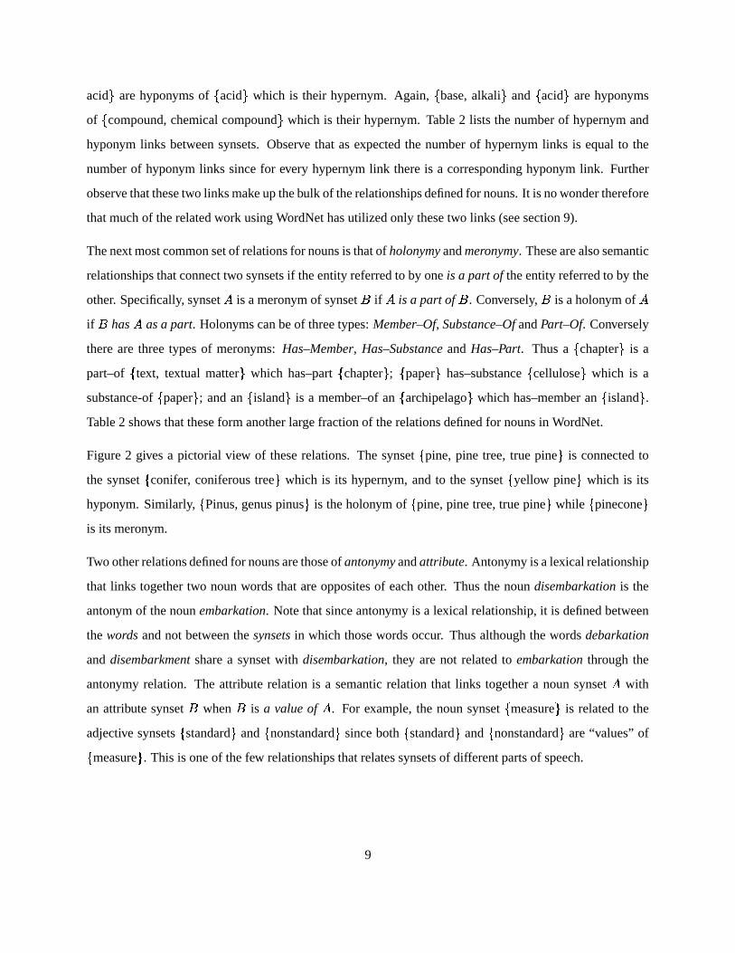
The next most common set of relations for nouns is that of holonymy and meronymy. These are also semantic

relationships that connect two synsets if the entity referred to by one is a part of the entity referred to by the

other. Specifically, synset�

is a meronym of synset � if�

is a part of � . Conversely, � is a holonym of�

if � has�

as a part. Holonyms can be of three types: Member–Of, Substance–Of and Part–Of. Conversely

there are three types of meronyms: Has–Member, Has–Substance and Has–Part. Thus a�chapter

�is a

part–of�text, textual matter

�which has–part

�chapter

�;�paper

�has–substance

�cellulose

�which is a

substance-of�paper

�; and an

�island

�is a member–of an

�archipelago

�which has–member an

�island

�.

Table 2 shows that these form another large fraction of the relations defined for nouns in WordNet.

Figure 2 gives a pictorial view of these relations. The synset�pine, pine tree, true pine

�is connected to

the synset�conifer, coniferous tree

�which is its hypernym, and to the synset

�yellow pine

�which is its

hyponym. Similarly,�Pinus, genus pinus

�is the holonym of

�pine, pine tree, true pine

�while

�pinecone

�

is its meronym.

Two other relations defined for nouns are those of antonymy and attribute. Antonymy is a lexical relationship

that links together two noun words that are opposites of each other. Thus the noun disembarkation is the

antonym of the noun embarkation. Note that since antonymy is a lexical relationship, it is defined between

the words and not between the synsets in which those words occur. Thus although the words debarkation

and disembarkment share a synset with disembarkation, they are not related to embarkation through the

antonymy relation. The attribute relation is a semantic relation that links together a noun synset�

with

an attribute synset � when � is a value of�

. For example, the noun synset�measure

�is related to the

adjective synsets�standard

�and

�nonstandard

�since both

�standard

�and

�nonstandard

�are “values” of

�measure

�. This is one of the few relationships that relates synsets of different parts of speech.

9

Table 2: Distribution of the various relationships for each part of speech.

Relationship (Type) Nouns Verbs Adjectives Adverbs

Hypernym (s) 76226 (38.7%) 12155 (45.5%) – –

Hyponym/Troponym (s) 76226 (38.7%) 12155 (45.5%) – –

Meronym (s) 20837 (10.6%) – – –

Holonym (s) 20837 (10.6%) – – –

Antonym (l) 1946 (1.0%) 1075 (4.0%) 4132 (12.0%) 720 (18.5%)

Attribute (s) 650 (0.4%) – 650 (1.9%) –

Entailment (s) – 426 (1.1%) – –

Cause (s) – 216 (1.6%) – –

Also see (l/s) – 611 (2.3%) 2714 (7.9%) –

Similar to (s) – – 22492 (65.1%) –

Participle of (l) – – 120 (0.3%) –

Pertainym of (l) – – 4433 (12.8%) 3174 (81.5%)

Totals 196722 26638 34541 3894

10

2.2 Verbs in WordNet

Two major relations defined for verbs in WordNet are hypernymy and troponymy. These are semantic re-

lations and are analogous to the noun hypernymy and hyponymy relations respectively. Synset�

is the

hypernym of � , if � is one way to�

; � is then the troponym of�

. Thus, the verb synset�station, post,

base, send, place�

is the troponym of�move, displace

�since to

�station, post, base, send, place

�is one way

to�move, displace

�. Table 2 shows that these two relationships form the lion’s share of the relations defined

for verbs in WordNet.

Like nouns, verbs are also related through the relationship of antonymy that links two verbs that are oppo-

site to each other in meaning. Thus the verb go which means to move away from a place into

another direction is the antonym of the verb come which means to move toward, travel

toward something or somebody. This is a lexical relationship, and does not apply to the other

words in the synsets that go and come belong to.

Other relations defined for verbs include those of entailment and cause, both of which are semantic relations.

A synset�

is related to synset � through the entailment relationship if�

entails doing � . Thus the verb

synset�walk

�has an entailment relationship with the take a step meaning of the verb synset

�step

�,

since walking entails stepping. A synset�

is related to synset � by the cause relationship if�

causes � .

For example,�embitter

�is related to

�resent

�because something that embitters causes one to resent.

The last relationship defined for verbs is that of also–see. We are unsure of the exact criteria for deciding

whether two synsets should have this relationship but believe that human judgment was used to make this

decision on a case–by–case basis. Also–see relationships can be either semantic or lexical in nature. For

instance the synset�enter, come in, get into, get in, go into, go in, move into

�which means to come

or go into is related to the synset�move in

�which means to occupy a place through the also–see

relation. In this case, since it is a semantic relation, every synset member of the synset�enter, come in,

get into, get in, go into, go in, move into�

is related to�move in

�through this relation. On the other hand

the verb sleep meaning to be asleep is related to the verb sleep in meaning to live in the house

where one works through a lexical also–see relationship. This is lexical since although the verb sleep

occurs in the synset�sleep, kip, slumber, log Z’s, catch some Z’s

�and sleep in occurs in the synset

�live in,

sleep in�, the rest of the members of the synsets are not related by an also–see relationship.

11

2.3 Adjectives and Adverbs in WordNet

Adjectives and adverbs in WordNet are fewer in number than nouns and verbs, and adverbs have far fewer

relations defined for them compared to the rest of the parts of speech.

The most frequent relation defined for adjectives is that of similar to. This is a semantic relationship that

links two adjective synsets that are similar in meaning, but not close enough to be put together in the same

synset. For example consider the following four synsets:�last

�with gloss immediately past,

�past

�

with gloss earlier than the present time,�last

�with gloss occurring at the time

of death and�dying

�with gloss in or associated with the process of passing

from life or ceasing to be. WordNet defines a similar to relation between the first two synsets

and another similar to relation between the third and fourth synsets. As with the also–see relationships, we

are unsure of the criteria for deciding similarity but believe that human judgment was used to decide if two

synsets should be linked through this relation. [Note that although the two synsets�last

�have exactly the

same members, they are still two distinct synsets with two distinct definitional glosses and different sets of

relationships etc.]

As mentioned previously, the attribute relationship links together noun and adjective synsets if the adjective

synset is a value of the noun synset. This is a symmetric relationship implying that for every attribute relation

that links a noun synset to an adjective synset, there is a corresponding attribute relation that connects the

adjective synset to the noun synset. Hence there are an equal number of attribute links for both nouns and

adjectives, as shown in table 2.

Adjectives also have a large number of also–see relationships defined for them in a manner similar to the

also–see relations for verbs. However unlike verbs, all also–see links between adjectives are semantic in

nature, and there are no lexical also–see relations for adjectives. For example the capable of being

reached sense of�accessible

�is connected to the suited to your comfort or purpose or

needs sense of�convenient

�through a semantic also–see relation.

The relationship of participle of is unique to adjectives, and links adjectives to verbs. This is a lexical

relationship and is defined between words and not between synsets. Thus the adjective applied is a participle

of the verb apply. As before, since this is a lexical relationship, it does not apply to the other members of

the synsets that these two words belong to. Further note that this is one of those rare relations that connects

12

words of two different parts of speech.

As with nouns and verbs, the relationship of antonymy links together words that are opposite in meaning to

each other for both adjectives and adverbs. Thus, the adjective wise is the antonym of the adjective foolish

while the adverb wisely is the antonym of the adverb foolishly. Recall that antonymy is a lexical relationship

and relates together individual words and not the synsets they belong to.

Finally the lexical relationship pertainym of relates adjectives to other adjectives and nouns, and relates

adverbs to adjectives. An adjective�

is related to another adjective or to a noun � if�

pertains to � . For

example the adjective bicentennial pertains to the adjective centennial which pertains to the noun century.

For adverbs, pertainym relations link adverbs to adjectives that they pertain to. For example, the adverb

animatedly pertains to the adjective animated. Note that this is the third relationship that crosses part of

speech boundaries to relate adjectives and adverbs to nouns.

13

3 Data for Experimentation

We evaluate the algorithms developed in this thesis using the data created as a part of the SENSEVAL-2

[9] comparative evaluation of word sense disambiguation systems. This is a large amount of high–quality

hand–tagged data where the sense–tags are taken from WordNet version ��� � . A large number of contesting

teams have evaluated their algorithms on this data, and the results of these evaluations are freely available

for us to compare our results against.

There were two separate sets of data available for English: the English lexical sample data and the English

all–words data. Although our algorithm can be applied to the all–words data too, we have only used the

lexical sample data for evaluation, and we describe this part of the data below.

The English lexical sample data consists of two sets of data: the training set and the test set. The training

data was used by to train the supervised algorithm of the participants of the SENSEVAL–2 exercise. Since

our algorithm uses an unsupervised methodology, we do not utilize the training data, and therefore describe

below only the test data.

The lexical sample test data consists of ��� tasks where each task consists of many occurrences of a single

target word that needs to be disambiguated. Except for a handful of exceptions, all the target words within

a single task are all used in the same part of speech. For example the art task consists of �� occurrences of

the target word art, all belonging to the noun part of speech. Each occurrence of the target word is called an

instance and consists of the sentence containing the target word as well as one to three surrounding sentences

that provide the context for the target word.

For example, the following is a typical instance from the art task. The symbols <head> and </head>

around the word Art specify that this occurrence of the word needs to be disambiguated.

Mr Paul, for his part, defends the Rubens price, saying a lot of the experts have never seen the

thing itself. “Most of them weren’t even born the last time the painting was displayed publicly,”

he says. <head>Art</head> prices are skyrocketing, but a good deal of legerdemain is

involved in compiling statistics on sales.

Each such instance of the target word is tagged by a human lexicographer with one or more sense–tags that

14

specify the sense(s) in which this word is being used in the given context. Note that the human tagger is

allowed to tag a word with more than one sense if she feels that the word is being used in multiple senses in

the present context. These sense–tags uniquely identify synsets in WordNet and it is the goal of Word Sense

Disambiguation systems to return these sense–tags. Each instance has a unique identifier and a separate

key file pairs these identifiers with their appropriate sense–tags. For example the above instance has the

id art art.30016, and the key file has the line art art.30016 art%1:06:00:: which implies

that the occurrence of the word art in this instance is intended to mean the WordNet sense identified by the

sense–tag art%1:06:00:: which means the products of human creativity; works of

art collectively.

Tasks are grouped according to the part of speech of their target word into three sets – nouns, verbs and

adjectives. Table 3 lists the tasks according to the part–of–speech of their target words, and the number of

instances within each task. The table also lists the number of senses defined for each target word in WordNet

within its given part of speech, and also the number of distinct sense–tags used to tag the various instances

of the task. Note that these are not the same numbers. It is possible that only a subset of the various senses

of a word defined in WordNet appear in the test data. This is because some senses of some words are very

rare, and the data does not contain examples of such usages. This is particularly true of verbs which have

a large number of senses defined in WordNet. On the other hand, it is also possible that a target word be

tagged with a sense that is not one of the senses of the word itself. This is particularly true when the target

word is tagged with the sense of one of the compound words that contain the target word. For example,

consider the following instance:

Most, if not all, of the martial <head>arts</head> are inextricably linked to the three main

East Asian religions, Buddhism, Taoism and Confucianism

arts here is tagged with a sense–tag that refers to the synset�martial art

�whose gloss is any of several

Oriental arts of weaponless self-defense. Observe that�martial art

�is a separate synset

by itself. Although art just has 4 senses, various instances of the art task are tagged with other senses such

as art collection, work of art, art dealer etc. Indeed, figuring out the candidate senses for our algorithm to

choose from is a non–trivial issue that we seek to address in section 5.

The various instances within a task are not related to each other. That is, although the sentences within a

15

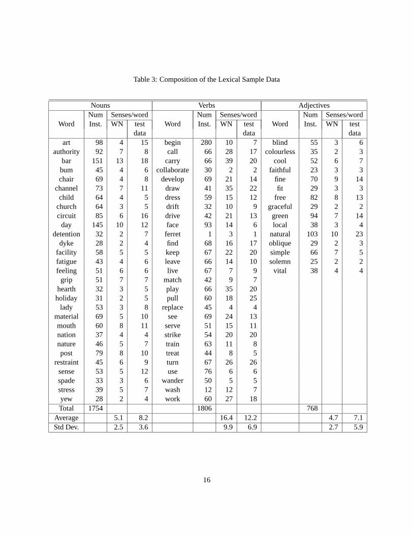
Table 3: Composition of the Lexical Sample Data

Nouns Verbs AdjectivesNum Senses/word Num Senses/word Num Senses/word

Word Inst. WN test Word Inst. WN test Word Inst. WN testdata data data

art 98 4 15 begin 280 10 7 blind 55 3 6authority 92 7 8 call 66 28 17 colourless 35 2 3

bar 151 13 18 carry 66 39 20 cool 52 6 7bum 45 4 6 collaborate 30 2 2 faithful 23 3 3chair 69 4 8 develop 69 21 14 fine 70 9 14

channel 73 7 11 draw 41 35 22 fit 29 3 3child 64 4 5 dress 59 15 12 free 82 8 13

church 64 3 5 drift 32 10 9 graceful 29 2 2circuit 85 6 16 drive 42 21 13 green 94 7 14

day 145 10 12 face 93 14 6 local 38 3 4detention 32 2 7 ferret 1 3 1 natural 103 10 23

dyke 28 2 4 find 68 16 17 oblique 29 2 3facility 58 5 5 keep 67 22 20 simple 66 7 5fatigue 43 4 6 leave 66 14 10 solemn 25 2 2feeling 51 6 6 live 67 7 9 vital 38 4 4

grip 51 7 7 match 42 9 7hearth 32 3 5 play 66 35 20

holiday 31 2 5 pull 60 18 25lady 53 3 8 replace 45 4 4

material 69 5 10 see 69 24 13mouth 60 8 11 serve 51 15 11nation 37 4 4 strike 54 20 20nature 46 5 7 train 63 11 8post 79 8 10 treat 44 8 5

restraint 45 6 9 turn 67 26 26sense 53 5 12 use 76 6 6spade 33 3 6 wander 50 5 5stress 39 5 7 wash 12 12 7yew 28 2 4 work 60 27 18Total 1754 1806 768

Average 5.1 8.2 16.4 12.2 4.7 7.1Std Dev. 2.5 3.6 9.9 6.9 2.7 5.9

16

single instance belong to the same topic and are a continuation of each other, sentences from two different

instances in general are neither continuations of each other nor do they necessarily belong to the same

topic. Note that barring a handful of instances ( ����� of the ��������� total instances), in every instance separate

sentences are on separate lines. Thus the data is mostly sentence boundary detected, that is for most of the

data the end of a sentence is marked by a new line character. We however do not make use of this piece of

information in our algorithms.

17

4 The Lesk Algorithm

4.1 The Algorithm

The original Lesk algorithm [11] disambiguates words in short phrases. Given a word to disambiguate, the

dictionary definition or gloss of each of its senses is compared to the glosses of every other word in the

phrase. A word is assigned that sense whose gloss shares the largest number of words in common with

the glosses of the other words. The algorithm begins anew for each word and does not utilize the senses it

previously assigned.

[11] demonstrates this algorithm on the words pine cone. Using the Oxford Advanced Learner’s Dictionary,

it finds that the word pine has two senses:

Sense 1: kind of evergreen tree with needle–shaped leaves

Sense 2: waste away through sorrow or illness.

The word cone has three senses:

Sense 1: solid body which narrows to a point

Sense 2: something of this shape whether solid or hollow

Sense 3: fruit of certain evergreen tree

Each of the two senses of the word pine is compared with each of the three senses of the word cone and it

is found that the words evergreen tree occurs in one sense each of the two words. These two senses are then

declared to be the most appropriate senses when the words pine and cone are used together.

Similarly the algorithm has been shown to correctly disambiguate the word flies in both time flies like an

arrow and fruit flies like a banana. Given a phrase like time flies like an arrow the algorithm compares the

glosses of all the sense of time to the glosses of all the senses of fly and arrow, and assigns to time that sense

that leads to the greatest number of overlapped words. Next it compares the glosses of fly with those of time

and arrow, and so on.

18

4.2 Implementation of the Algorithm

Two variations of the Lesk algorithm were presented at the SENSEVAL–2 exercise. The first counted the

number of words in common between the instance in which the target word occurs and its gloss. Each

word count was weighted by its inverse document frequency which was defined simply as the inverse of the

number of times the word has occurred in the instance or the gloss in which the word occurs. The gloss

with the highest number of words in common with the instance in which the target word occurs represents

the sense assigned to the target word. This approach achieved �� ��� overall accuracy. A second approach

proceeded identically, except that it added example texts that WordNet provides to the glosses. This achieved

accuracy of ��� ��� suggesting that the example strings associated with the various synsets is a potential source

of useful information.

Since low–level implementation details can significantly alter results, we however decided to re–implement

the Lesk algorithm. This gives us a uniform platform to compare the accuracy of the Lesk algorithm with

that obtained by our modified algorithms.

The original Lesk paper [11] disambiguates words in phrases or short sentences. The SENSEVAL–2 data

however consists of long sentences and using all the words in them would quickly become computationally

intensive. Hence we define a short window of context around the target word, and submit all the words in

this window as input to the disambiguation algorithm. We define a window of ������� � words around

the target word to include the target word and � words to its left and right. In doing so, we do not respect

sentence boundaries and if need be, select words that belong to sentences that surround the one containing

the target word. We do so since the words in the surrounding sentences are also related to the target word

and can help in its disambiguation.

Since our algorithm is dependent on the glosses of the words in the context window, words that do not occur

in any synset in WordNet are ignored. This rules out function words like the, of, an, etc and also most proper

nouns. If not enough words exist to the left or right of the target word, we add additional words from the

other direction. This is an attempt to provide roughly the same amount of data for every target word. For our

experiments we use a window size of � � words. Thus our window is usually made up of � words to the left

of the target word, � words to the right and the target word itself. This number is used for historical reasons

– it is the largest odd number less than or equal to the number of content words in the longest sentence

19

disambiguated in the Lesk paper [11].

As an example of how a window of 11 words may be selected around the target word, consider the following

instance of the art task:

Mr Paul, for his part, defends the Rubens price, saying a lot of the experts have never seen the

thing itself. “Most of them weren’t even born the last time the painting was displayed publicly,”

he says. <head>Art</head> prices are skyrocketing, but a good deal of legerdemain is

involved in compiling statistics on sales.

Given this instance, and that the target word is art, the window of 11 words would be the words painting

was displayed publicly says Art prices are skyrocketing but good.

Given a window of words, we compare the gloss of each sense of the target word with the concatenation of

the glosses of all the other words in the window. The number of words found to be common to these two

strings of words is declared to be the score of the sense of the target word. That sense that has the highest

score is declared the most appropriate one for the target word in the given context.

Appendix A contains the pseudo code for this algorithm.

4.3 Evaluation of the Algorithm

As mentioned before, we evaluate this algorithm and other algorithms on the SENSEVAL-2 English lexical

sample data. Recall that the lexical sample data consists of instances that are 2 to 3 sentences long and

contain exactly one target word that must be disambiguated. The human lexicographer–decided senses for

each target word in the data is available to us.

Given the senses returned by our system we compute precision � as the number of target words for which

our answer matches the human decided answer, divided by the number of instances for which answers have

been returned by our system. Note that our system does not return answers for target words that do not have

any overlaps for any of their senses since the absence of overlap implies the absence of evidence for any

particular sense. Thus the number of target words for which we have answers may be less than the total

number of target words. We compute recall � as the number of target words in which our answer matches

20

Table 4: Pure Lesk Evaluation

Part of Speech Precision Recall F–Measure

Lexical Sample 0.183 0.183 0.183

Noun 0.258 0.258 0.258

Verb 0.116 0.116 0.116

Adjective 0.170 0.170 0.170

that of the humans divided by the total number of target words in the data. Having calculated precision and

recall, we compute F–measure as � � � � ����

��� ��� . The F–measure [16] is a standard way of combining

the precision and recall values into a single figure and is in fact the harmonic mean of these two values with

equal weightage given to both precision and recall.

Table 4 shows the precision, recall and f–measure for target words belonging to the English lexical sample

data. Recall that this data is split into three groups depending on the part of speech of the target word. The

table shows the precision / recall / f–measure values for each of these groups as well as the overall values

for the whole of the lexical sample data.

We observe that our implementation of the Lesk algorithm achieves precision of about 0.183. Further, it

achieves precision of 0.258 on the noun tasks, 0.17 on the adjectives but only 0.116 on the verbs. Recall

from table 1 that in general verbs have both the shortest glosses and the largest number of senses as compared

to nouns and adjectives. We surmise that this is perhaps the reason for the relatively poor results on the verbs,

as compared to the nouns and adjectives. In the next sub–section we compare these results with other results

obtained on the same data to put these results in perspective.

4.4 Comparison with Other Results

Tables 5 show the precision, recall and f–measure values achieved by the participants of the SENSEVAL–2

competition. These values are obtained from http://www.sle.sharp.co.uk/senseval2. Recall

that for the lexical sample data, a large amount of sense–tagged data on each task (8599 instances for the

73 tasks) was available as a separate training set before the actual test data was available. This data was

21

Table 5: Performance of Senseval–2 participants using an unsupervised approach on the English lexical

sample data.

Team Name Precision Recall F–Measure

UNED - LS-U 0.402 0.401 0.401

WordNet ����

Sense 0.383 0.383 0.383

ITRI - WASPS-Workbench 0.581 0.319 0.412

CL Research - DIMAP 0.293 0.293 0.293

IIT 2 (R) 0.247 0.244 0.245

IIT 1 (R) 0.243 0.239 0.241

IIT 2 0.233 0.232 0.232

IIT 1 0.220 0.220 0.220

Our Lesk implementation 0.183 0.183 0.183

Random 0.141 0.141 0.141

used by participants taking a supervised approach to WSD. The highest precision and recall achieved by the

supervised approaches was around ��������

. Teams that took an unsupervised approach however elected to

not use this data. Since our algorithm also uses an unsupervised approach, we show in table 5 the precision,

recall and f–measure values achieved by the unsupervised participants only.

The table also shows the results of applying two other baseline algorithms – the WordNet ����

sense baseline

and the random sense baseline. These results are shown in bold–face in table 5. Recall that senses in

WordNet are stored in approximate frequency of usage as observed in SemCor [14] which is a large corpus

of manually hand–tagged text. WordNet ����

sense results are obtained by assigning to each target word the

first sense of that word as listed in WordNet. Since we were given the part of speech of the target words in

the lexical sample tasks, we assigned to a target word the first of the senses within its given part of speech.

In the random sense baseline, one of the various possible senses of the target word is picked at random and

assigned to the word.

Observe that our implementation of the baseline Lesk algorithm achieves a recall that is greater than that of

the random algorithm. Since the random algorithm is an exceedingly cheap solution, this is the minimum

22

that we could ask of an algorithm. Interestingly, several systems got worse than random recall on the all–

words data. However these systems achieved higher precision than the random algorithm implying that they

sacrifice high recall for high precision.

However the precision and recall values of the Lesk algorithm are much lower than those of the WordNet

����

sense algorithm on both sets of data. This is true of the other systems too. For example, only 1 out of

the 7 teams achieved higher recall than this baseline. We believe that the difficulty in beating this baseline

lies in the fact that these values were obtained by utilizing data from a large amount of human sense–tagged

text and hence rightfully belongs to the domain of supervised statistical disambiguation.

For the lexical sample data, although the Lesk algorithm gets a higher recall than the random algorithm, it

achieves worse results than every other participating team.

While the precision / recall values achieved by the Lesk algorithm are greater than those achieved by a

random algorithm and hence represent some degree of effectiveness, it is far from the best. We believe

that this poor showing can be partially attributed to the brevity of definitions in WordNet in particular and

dictionaries in general. The Lesk algorithm is crucially dependent on the lengths of glosses. However

lexicographers aim to create short and precise definitions which, though a desirable quality in dictionaries,

is disadvantageous to this algorithm. Table 1 shows that on average glosses are between 4 to 11 words long.

Observe further that nouns have the longest glosses, and indeed the highest precision and recall obtained

is on nouns. Further, the normal Lesk algorithm was not designed keeping the hierarchical structure of

WordNet in mind. In the next section, we augment the glosses of the words by utilizing the semantic

hierarchy of WordNet, and show that this improves the accuracy of the disambiguation system.

23

5 Global Disambiguation Using Glosses of Related Synsets

5.1 Our Modifications to the Lesk Algorithm

We modify the Lesk algorithm in several ways to create our baseline algorithm. Like our implementation

of the Lesk algorithm, the basic unit of disambiguation of our algorithm continues to be a short window of

context centered around the target word. Unlike the Lesk algorithm though where we use a window of � �

words, for our adapted algorithm we restrict ourselves to a very short window of only � words. That is, our

context window is made up of the target word together with the first words that occur to its left and right

in the instance. Our choice of such a short window is partly motivated by [4] who find that human beings

generally use the immediate context of a word for disambiguation. We are also required to choose such a

short window due to computational reasons as discussed below. Thus, although [4] report a window of 5

words as being sufficient for disambiguation, we have had to experiment with only a 3 word window. We

modify our algorithm to relax this constraint in later experiments (see section 6).

5.1.1 Choice of Dictionary

The original Lesk algorithm relies on glosses found in traditional dictionaries such as Oxford Advanced

Learner’s Dictionary of Current English, Webster’s 7th Collegiate, Oxford English Dictionary, Collins En-

glish Dictionary etc. We on the other hand choose the lexical database WordNet to take advantage of the

highly inter–connected set of relations among different words that WordNet offers.

5.1.2 Choice of Which Glosses to Use

While Lesk’s algorithm restricts its comparisons to just the dictionary meanings of the words being disam-

biguated, our choice of dictionary allows us to also compare the meanings (i.e., glosses) of words that are

connected to the words to be disambiguated through the various relationships defined in WordNet. This

provides a richer source of information and, we show, improves disambiguation accuracy.

For the various comparisons in our experiments, we utilize the glosses of the various synsets that the word

belongs to, as well as the glosses of those synsets that are related to them through the relations shown in

24

table 6. We base our choice of relations on the statistics shown in table 2. For each part–of–speech we use

a relation if links of its kind form at least 5% of the total number of links for that part of speech, with two

exceptions.

We use the attribute relation although there are not many links of its kind. Recall that this relation links

adjectives, which are not well developed in WordNet, to nouns which have a lot of data about them. This

potential to tap into the rich noun data prompted us to use this relation. The other exception is the antonymy

relationship. Although there are sufficient antonymy links for adjectives and adverbs, in our experiments we

have not utilized these relations; these relations may be included in further experiments.

Besides these relations, we choose the hypernym, hyponym/troponym links for both nouns and verbs. Recall

that these links create the is a hierarchy, which has been used by several researchers in the past for word

sense disambiguation (see chapter 10). Further these relations are quite abundant, making them a very

attractive source of information. The is a part of and has a part hierarchy built on the holonym/meronym

links is another informative and richly developed relationship for nouns, and so we use those links as well.

For verbs, we avoid the cause and entailment relations since they make up less than 2% of the total links

for verbs. We elect instead to use the also–see relation that links together related words. We are not sure if

these links overlap to a large extent with the hypernym/troponym relations thereby rendering them redundant

when used with hypernyms and troponyms. However, if indeed using the also–see links is the same as using

the hypernym links twice, we do not see this as a problem for the disambiguating algorithm except in its

computationally intensive aspect.

For adjectives, we use the attribute relation for reasons mentioned above. We also make use of the also–see

and similar–to relations which link together related words and together account for more than 80% of the

links defined for adjectives, as shown in table 2. We also utilize the pertainym–of links which form more

than 8% of adjective links.

5.1.3 Schemes for Choosing Gloss–Pairs to Compare

We shall henceforth denote word senses in the word#pos#sense format. For example, we shall denote by

sentence#n#2 the second sense of the noun sentence. The numbering of the senses is unimportant in our

discussion here, and will be used merely to distinguish between different senses of the same word within a

25

Table 6: Relations Chosen For the Disambiguation Algorithm

Noun Verb AdjectiveHypernym Hypernym AttributeHyponym Troponym Also seeHolonym Also see Similar toMeronym Pertainym ofAttribute

given part–of–speech. Note that each such word#pos#sense string belongs to exactly one synset in WordNet.

Thus, this string may be used to uniquely identify a synset in WordNet.

We shall denote by gloss(word#pos#sense) the gloss of the synset that word#pos#sense identifies. For

example:

gloss(sentence#n#2) = the final judgment of guilty in criminal cases and

the punishment that is imposed.

We shall denote by hype(word#pos#sense) all the hypernym synsets of the synset identified by word#pos#sense.

For example:

hype(sentence#n#2) =�string, string of words, word string, linguistic string

�.

Similarly, we shall denote by hypo(word#pos#sense) all the synsets that are related to the synset identified

by word#pos#sense through the hyponymy relationship. For example,

hypo(sentence#n#2) =�murder conviction

�,�rape conviction

�and

�robbery conviction

�.

To denote the gloss of the hypernym or hyponym of the synset identify by word#pos#sense, we shall use the

notation gloss(hype(word#pos#sense)) and gloss(hypo(word#pos#sense)) respectively. For example:

gloss(hype(sentence#n#2)) = a judgment disposing of the case before the

court of law.

26

If multiple hypernyms or hyponyms exist for the synset referred to by the string word#pos#sense, then

gloss(hype(word#pos#sense)) and gloss(hypo(word#pos#sense)) will be used to denote the concatenation

of the glosses of all those hypernyms and hyponyms respectively. For example:

gloss(hypo(sentence#n#2)) = conviction for murder conviction for rape

conviction for robbery.

We perform this concatenation since we do not distinguish between the various hyponym synsets of a given

synset, and wish to obtain a single string of words that represents the “hyponym gloss” of the synset under

consideration.

It is possible that the synset pointed to by word#pos#sense has no hypernyms. In that case,

hype(word#pos#sense) returns the empty set, and gloss(hype(word#pos#sense)) the empty string – and sim-

ilarly with hyponyms.

Say then that we wish to compare the ����

sense of the noun sentence, sentence#n#2 with the ����

sense of

the noun bench, bench#n#2. The original Lesk algorithm looks for overlaps between

gloss(sentence#n#2) = the final judgment of guilty in criminal cases and

the punishment that is imposed

and

gloss(bench#n#2) = persons who hear cases in a court of law.

Observe that besides function words like in and a, the only overlap here is the word cases, and so the Lesk

algorithm assigns a “score” of only � between two senses which are obviously much more strongly related

than what the overlaps show.

We consider not only the glosses of the synsets of the two words themselves, but also a large set of other

synsets related to these as listed above. For illustration purposes, consider for the moment only the hypernym

and hyponym synsets. Associated to sentence#n#2 therefore, we have three glosses: gloss(sentence#n#2),

gloss(hype(sentence#n#2)) and gloss(hypo(sentence#n#2)). Associated with bench#n#2 we have only two

27

"persons who hear

{final judgement, final decision}

before the court of law""a judgement disposing of the case

{rape conviction}, {robbery conviction}"conviction for murder; conviction for rape

{murder conviction}

conviction for robbery"

hype(sentence#n#2)

sentence#n#2

hypo(sentence#n#2)

{sentence, conviction, judgement of conviction}

the punishment that is imposed""the final judgment of guilty in criminal cases and

{administration, governance, establishment}"the persons who make up a governing body and

who administer something"

{bench, judiciary}

court of law"cases in a

hype(bench#n#2)

bench#n#2

Figure 3: Heterogeneous scheme of selecting synset pairs for gloss–comparison. Ovals denote synsets,

with synset members in���

and the gloss in quotation marks. Dotted lines represent the various gloss–gloss

comparisons. Overlaps are shown in bold.

glosses, gloss(bench#n#2) and gloss(hype(bench#n#2)), since bench#n#2 does not have a hyponym. Given

this bunch of glosses, we need to decide how to select pairs of glosses for comparison.

We experiment with two possibilities that we call the heterogeneous and the homogeneous schemes of

gloss–pair selection. In the heterogeneous scheme, we compare every gloss associated with the sense under

consideration of the first word with every gloss associated with that of the second. In our example therefore,

we perform 6 comparisons by comparing in turn each of the three glosses associated with sentence#n#2 with

each of the two associated with bench#n#2.

Fig. 3 shows this scheme diagrammatically. Observe that besides the one word overlap of the word cases

between gloss(sentence#n#2) and gloss(bench#n#2), there is a three word overlap court of law between

hype(gloss(sentence#n#2)) and gloss(sentence#n#2), confirming the fact that these two senses are indeed

strongly related to each other.

In the homogeneous scheme of synset–pair selection, to compare two senses of two words, we look for

overlaps between their glosses, and also between glosses of synsets that are related to these senses through

the same relation. In our example therefore, we perform only two comparisons: gloss(sentence#n#2) with

28

gloss(bench#n#2), and gloss(hype(sentence#n#2)) with gloss(hype(bench#n#2)).

These are shown in figure 4. Observe that unlike in the heterogeneous scheme, we now have only one

overlap cases. However, also note that in the homogeneous scheme, far fewer comparisons are performed.

In general, assume that there are ��� � synsets related to the sense of the first word and � � � to the second

word. While the heterogeneous scheme performs � � � comparisons, the homogeneous scheme performs

only ��� ��� � � � .

Observe that the homogeneous scheme is a more direct extension of the original Lesk algorithm. Recall that

the original Lesk algorithm compares only the definitions of the words being disambiguated. In a similar

vein, in the homogeneous scheme we compare the definitions of the words in the context window and the

definitions of only those words that are related to them through the same relationship. In the heterogeneous

scheme on the other hand, the definitions of every word related to a single word in the window is compared to

the definitions of every word related to another word in the window in a bid to observe all possible overlaps

and relationships between the two words.

"persons who hear

hype(bench#n#2)

bench#n#2

hype(sentence#n#2)

sentence#n#2

hypo(sentence#n#2)

{sentence, conviction, judgement of conviction}

the punishment that is imposed""the final judgment of guilty in criminal cases and

{bench, judiciary}

court of law"cases in a

{rape conviction}, {robbery conviction}"conviction for murder; conviction for rape

{murder conviction}

conviction for robbery"

{final judgement, final decision}

before the court of law""a judgement disposing of the case

{administration, governance, establishment}"the persons who make up a governing body and

who administer something"

Figure 4: Homogeneous scheme of selecting synset pairs for gloss–comparison. Ovals denote synsets, with

synset members in���

and the gloss in quotation marks. Dotted lines represent the various gloss–gloss

comparisons. Overlaps are shown in bold.

29

5.1.4 Overlap Detection between Two Glosses

When comparing the dictionary definitions or glosses of two words, the original Lesk algorithm counts up

the number of tokens that occur in both glosses and assigns a score equal to the number of words thus

matched to this gloss–pair. We introduce a novel overlap detection and scoring mechanism that looks for

longer multi–word sequences of matches, and weighs them more heavily than shorter matches.

Specifically, when comparing two glosses, we define an overlap between them to be the longest sequence

of one or more consecutive words that occurs in both glosses such that neither the first nor the last word is a

function word, that is a pronoun, preposition, article or conjunction. If two or more such overlaps have the

same longest length, then that overlap that occurs earliest in the first string being compared is reported.

Given two strings, the longest overlap between them is detected, removed and in its place a unique marker

is placed in each of the two strings. The two strings thus obtained are then again checked for overlaps, and

this process continues until there are no longer any overlaps between them. All the overlaps found in this

process are reported as the overlaps of the two strings.

For example assume our strings are the following:

First string: this is the first string we will compare

Second string: I will compare the first string with the second

Observe that there are two overlaps of size two words each: first string and will compare. Since first string

occurs earlier than will compare in the first string, we report first string as the first overlap. We remove this

overlap and replace it with markers M1 and M2 in the two strings respectively, thereby getting the following

strings:

First string: this is the M1 we will compare

Second string: I will compare the M2 with the second

We attempt to find overlaps in these two strings, and find the overlap will compare which we replace with

markers.

30

First string: this is the M1 we M3

Second string: I M4 the M2 with the second

Observe that there are no overlaps left in these two strings, and so we report first string and will compare as

the overlaps between these two strings.

Note that by replacing overlaps by unique markers we prevent spurious overlaps comprising of words on the

two sides of the previously detected and removed overlap. Further note that our decision to rule out overlaps

that start and end with function words effectively rules out all overlaps that consist entirely of function

words. Thus, overlaps like of the, on the etc. are ruled out since such overlaps do not seem to contain

any information that would help disambiguation. Further, given an overlap like the United States

of America, our definition requires us to ignore the the, and consider only United States of

America as an overlap. We do not believe that adding the function word to the front of the overlap gives it

any extra information, and hence the decision to ignore it.

Overlaps that start and end with content words, but have function words within them are retained. This is to

preserve longer sequences, as opposed to breaking them down into smaller sequences due to the presence

of function words. Thus, although of is a function word, we would still consider United States of

America as a single overlap of four words.

As mentioned above, two glosses can have more than one overlap where each overlap covers as many

words as possible. For example, the sentences he called for an end to the atrocities

and after bringing an end to the atrocities, he called it a day have the fol-

lowing overlaps: end to the atrocities and he called.

Note also that our definition requires us to look at words for matching, and prevents us from reporting partial

word matches. Thus for example, between Every dog has his day and Don’t make hasty

decisions, there exists an overlap of the letters h-a-s, which we do not report. A special case of this

problem occurs when the same word occurs in two glosses with two different inflections. For example tree

and its plural trees. We handle this case by first preprocessing the glosses and replacing each word with

its WordNet stem. Recall that WordNet stores only stems of words, and not their various inflected forms.

Through a simple rule based procedure, it defines how inflected forms of words are mapped onto their stems.

We use this procedure to replace inflected words in the glosses with their stems. However, some words can

31

have multiple stems. For example axes could be the plural form of both axe as well as axis. In such cases,

one possibility is to replace the inflected form by a regular expression that includes both the stemmed forms

such that when matching is done, exactly one of them will get matched. Since we do simple string matching

however, we avoided this approach, and chose to simply leave the inflected word unchanged. Thus if the

word axes occurs in any gloss, it remains unchanged.

5.1.5 Using Overlaps to Measure Relatedness between Synsets

Having found one or more overlaps between two glosses, we need to quantify the amount of information

that we believe they convey about the relatedness of the two synsets being compared. The original Lesk

algorithm achieves this goal by counting up the number of words that have overlapped, and reporting this

count as a “score” between the two glosses being compared. We extend this mechanism by giving a higher

weight to multi–token overlaps.

Consider the following two sentences:

Sentence 1: you are the boy

Sentence 2: you are the boy I like

The overlap between these two sentences as found by the algorithm described above is you are the boy.

Since 4 words have overlapped between these two sentences, Lesk’s scoring mechanism would have given

them a score of 4. However in this computation, the fact that the overlap consists of one four–token long

phrase is lost. That is, this scoring mechanism would have given the same score to these two sentences had

the overlapped tokens been separated from each other and not occurred in one long phrase.

We wish to modify this scoring scheme in such a way that a gloss pair having an � token overlap gets a

higher score than if the same � tokens had occurred in two or more overlaps, each of size less than � . We

achieve this objective by squaring the number of tokens in an � token overlap while counting the number of

overlapped tokens between two sentences.

For instance, consider the previous example again. Instead of counting you are the boy as an overlap of 4,

we shall count this as an overlap of � � ��� ��� . This is higher than if these four tokens had occurred in two

overlaps of 1 and 3 tokens respectively (in which case the total score would have been�� � � � � � � � � ��� ��� ,

32

two overlaps of 2 and 2 tokens each (���� � � � �

��� � � � � ), three overlaps of 1, 1 and 2 tokens each

(�� � � � � � � � � � � � � � � ��� � ), etc.

By squaring � token overlaps, we appeal to Zipf’s Law [18] which states that the frequency of an event is

inversely proportional to the rank of that event, where the ranking is based on the frequencies of all events.

This implies that most events occur only once, and only a few occur with greater frequency. The occurrence

of individual words in a corpus of text holds to this distribution, and it also applies to the occurrence of

multi-word sequences. As word sequences grow longer, it is increasingly rare to observe them multiple

times in a corpus. Thus, if we find a multi-word match between two glosses, this is a remarkable event, and

merits more than a linear increase in scoring.

By squaring the length of the match, we give a higher score to a single � token sequence than to the combined

score of those � tokens if they were to occur in shorter sequences. This is due to the fact that the square of a

sum of positive integers is strictly greater than the sum of their squares. Algebraically,� ��� � ��� � � � � � �

�� ���

��� � �

�� � � � � � �

�

�, where � is a positive integer.

5.1.6 Global Disambiguation Strategy

The original Lesk algorithm disambiguates each word separately. That is, it looks at each word in the context

window, compares the gloss of each of its senses with the glosses of all the senses of all its surrounding

words, assigns that sense for the current word that produces the most matches, and then carries on, starting

afresh with the next word in the window. Thus the sense assigned to a single word does not depend on

knowing the particular senses of its neighbouring words. We call this the local approach. In a way, the

disambiguation of the various words in a sentence are a series of independent problems and have no effect

on each other.

We propose an approach where all the words in the context window are simultaneously disambiguated in a

bid to get the best combination of senses for all the words in the window instead of only the target word. We

call this the global approach. As opposed to the local approach discussed above, the sense chosen for the

target word depends on those chosen for the words around it, and vice versa.

In this approach a score is computed for every possible combination of senses, where each such combination

contains exactly one sense for each word in the context window, and is distinct from every other combina-

33

tion. Given a combination of senses, all possible pairs of senses are chosen from the combination. Every

such pair of senses is then scored by comparing the various glosses associated with them (using either the

homogeneous or heterogeneous scheme) and squaring and adding the lengths of the overlaps thus found.

The scores computed for all the pairs of senses within one combination are then added together to arrive at

the score for the combination. The highest scoring combination is picked as the most appropriate one and

each word in the window is assigned its corresponding sense in this winning combination. This algorithm is

also described in [2].

For example assume we have the following three words in our window of context: sentence, bench and

offender. Say that there are two senses of sentence that we shall denote by sentence#n#1 and sentence#n#2

respectively, two of bench, denoted by bench#n#1 and bench#n#2 respectively and one of offender denoted

by offender#n#1. Following are the glosses of these senses.

gloss(sentence#n#1) = a string of words satisfying the grammatical rules

of a language

gloss(sentence#n#2) = the final judgment of guilty in criminal cases and

the punishment that is imposed

gloss(bench#n#1) = a long seat for more than one person

gloss(bench#n#2) = persons who hear cases in a court of law

gloss(offender#n#1) = a person who transgresses law

Given these three words with two senses for the first word, two for the second and one for the third, there

are a total of 4 distinct combinations that can be formed. Following are the combinations, numbered in no

particular order:

Combination 1: sentence#n#1 – bench#n#1 – offender#n#1

Combination 2: sentence#n#1 – bench#n#2 – offender#n#1

Combination 3: sentence#n#2 – bench#n#1 – offender#n#1

Combination 4: sentence#n#2 – bench#n#2 – offender#n#1

Note that since the last word, offender has only one sense, it will be assigned that sense at the end of the

algorithm. However, we use the gloss of this sense of the word to help disambiguate the other two words so

34

Table 7: Computation of the Score for the Combination in Figs. 5 and 6

First Gloss Second Gloss Overlap String Normalized Score

hype(sentence#n#2) bench#n#2 court of law, case 10

sentence#n#2 bench#n#2 cases 1

hype(sentence#n#2) offender#n#1 law 1

sentence#n#2 hypo(offender#n#1) criminal 1

hype(bench#n#2) hype(offender#n#1) person 1

hype(bench#n#2 offender#n#1 person 1

hype(bench#n#2) hypo(offender#n#1) person 1

bench#n#2 hype(offender#n#1) person 1

bench#n#2 offender#n#1 person, law 2

bench#n#2 hypo(offender#n#1) person 1

Total score for sentence#n#2 – bench#n#2 – offender#n#1 20

that the chosen senses for them are the most appropriate when used in conjunction with the single sense of

the word offender.

For each of the combinations above, we can form 3 pairs of senses to compare. Figures 5 and 6 show

the pairs formed for the last combination, sentence#n#2 – bench#n#2 – offender#n#1. These figures also

show by the dotted arrows the comparisons made when using a heterogeneous scheme of gloss selection.

Thus, for each pair of senses, every gloss associated with the first sense is compared to every gloss asso-

ciated with the second one. Thus in our example, the three glosses associated with sentence#n#2 (namely

gloss(sentence#n#2), gloss(hype(sentence#n#2)) and gloss(hypo(sentence#n#2)) are compared to the two

associated with bench#n#2. Note that bench#n#2 does not have any hyponyms. Similarly, the glosses asso-

ciated with sentence#n#2 are compared to those associated with offender#n#1, and those of bench#n#2 with

those of offender#n#1.

Observe that there is a three–word overlap, court of law, and a one word overlap, case, between

gloss(hype(sentence#n#2)) and gloss(bench#n#2). This gives us a score of ��� �

�� ��� for this gloss pair.

The rest of the overlaps and their scores are shown in table 7.

35

"persons who hear

{administration, governance, establishment}"the persons who make up a governing body and

who administer something"

{bench, judiciary}

court of law"cases in a

hype(bench#n#2)

bench#n#2

{rape conviction}, {robbery conviction}"conviction for murder; conviction for rape

{murder conviction}

conviction for robbery"

Comparison between sentence#n#2 and bench#n#2

hype(sentence#n#2)

sentence#n#2

hypo(sentence#n#2)

{sentence, conviction, judgement of conviction}

the punishment that is imposed""the final judgment of guilty in criminal cases and

{final judgement, final decision}

before the court of law""a judgement disposing of the case

"person who transgresses

{rape conviction}, {robbery conviction}"conviction for murder; conviction for rape

{murder conviction}

conviction for robbery"

{convict}, {felon}{attacker},

"someone who attacks; person convicted

commits a crime"offence; someone whoof a criminal

hypo(offender#n#1)

hype(sentence#n#2)

sentence#n#2{sentence, conviction, judgement of conviction}

the punishment that is imposed"

{final judgement, final decision}"a judgement disposing of the case

before the court of law"

"the final judgment of guilty in criminal cases and

{bad person}"a person who does harm to others" hype(offender#n#1)

{wrongdoer, offender}law" offender#n#1

hypo(sentence#n#2)

Comparison between sentence#n#2 and offender#n#1

Figure 5: Comparisons involving the first two pairs of senses in the combination sentence#n#2 – bench#2#n

– offender#n#1. Ovals show synsets, with synset members in���

and the gloss in quotation marks. Dotted

lines represent the various gloss–gloss comparisons. Overlaps are shown in bold.

36

who hear cases in a

who transgresses

{bad person}hype(offender#n#1)

{wrongdoer, offender}law" offender#n#1

hype(bench#n#2)

bench#n#2{bench, judiciary}

{convict}, {felon}{attacker},

commits a crime"

hypo(offender#n#1)

{administration, governance, establishment}

of a criminal offence; someone who

who make up a governing bodyand who administer something"

"personscourt of law"

"person

persons"the

who does harm toothers"

person"a

Comparison between bench#n#2 and offender#n#1

"someone who attacks; convictedperson

Figure 6: Comparisons involving the third pair of senses in the combination sentence#n#2 – bench#2#n –

offender#n#1. Ovals show synsets, with synset members in���

and the gloss in quotation marks. Dotted

lines represent the various gloss–gloss comparisons. Overlaps are shown in bold.

37

Note that when using the words of a gloss for matching, the stop words at the beginning and the end of the

gloss will never be matched according to our definition of an overlap. Further note that although the word

person occurs in its plural form in gloss(bench#n#2), it still matches the singular form in gloss(hype(offender#n#1))

since they have the same stem. Recall that the glosses are pre–processed where inflected words are replaced

by their stems as defined in WordNet. Finally observe that although words like a and in also overlap between

the glosses being compared, these do not qualify as overlaps according to our definition of an overlap above.

Overlaps found in these comparisons are scored as described in section 5.1.5 above and these scores are

added together to arrive at the score for this combination. The score from each overlap is shown in table

7. Similar scores are obtained for the other three combinations, and the highest scoring combination is

reported as the most appropriate combination of senses for the words in the context window. As it turns out,

the combination of figs. 5 and 6 is the highest scoring combination, and is therefore considered the most

appropriate assignment of senses to the three words in the context window.

This approach is motivated by a suggestion in [11] that the choice of sense for a given word should depend on

the choices of senses for the other words in the context window. We try to achieve this desirable condition

by computing the appropriateness of a certain sense of the target word when juxtaposed with particular

senses of the non–target words. Further by comparing the non–target words, we hope to find strong overlaps

between them. We hypothesize that such strong overlaps between a particular sense each of two non–target

words imply that those are the appropriate sense for those words, and then those senses become the deciding

factor in choosing between the various senses of the target word.

However this assumption is appropriate only when the words being compared are very closely related to

each other. In our example above, one sense each of the words sentence, bench and offender are closely

related to the topic of law, and so it makes sense to compare them. This is usually true of words in queries

submitted to information retrieval systems. Queries are usually made of a few words such that one sense of

each is highly related to each other. In such situations, the global mechanism above will be very useful for

disambiguation.

Our data, however, is in the form of long sentences in which only a few words are related to the target word

strongly enough for this algorithm to work well. Unfortunately, we have no automatic way of deciding

beforehand which of the words in the sentences are so related, and hence we compare every word with

every other in the window in the hope that we shall be able to detect the useful relations. (See Future Work

38

however for one possible way of detecting which words make sense to be used for comparison).

Another disadvantage of this approach of comparing every sense of every word with every sense of every

other word in the context window is that it makes the algorithm very computationally intensive. Assuming

that there are � senses per word on average, and that there are�

words in the window of context, there are

���

��� �� � �

� (1)

pairs of sets of synsets to compare. The value of this formula is exponential with�

.

5.2 Evaluation of The Global Disambiguation Algorithm

We evaluate our baseline algorithm on the SENSEVAL–2 lexical sample data. Recall that this data consists

of instances where each instance contains 2 to 3 sentences that are a continuation of each other. Exactly

one word in each instance is demarcated as the target word – the goal of our algorithm is to predict the

sense of this word. The sentences in an instance make up the context of the target word and can be used to

disambiguate it.

5.2.1 Preprocessing the Data

We subjected the context of each instance of the SENSEVAL–2 data to several pre–processing steps before

running the baseline algorithm, the first of which involved the identification of WordNet compound words.

Recall that besides individual words, WordNet also stores information on a large number of compound–

words that are multi–word sequences treated at par with single words. Often, these are proper nouns like

New York City or phrases like pull the leg of whose meanings are different from those of the component

words. WordNet treats these compounds on the same level as other individual words, with their own senses

and synsets.

We assume that if two or more consecutive words in a given text form a compound in WordNet, then these

words are indeed being used as compounds rather than individual words. Thus for example in the sentence

My friend is an art historian, we replace the two words art historian with the single compound art historian

since this is a compound recognized by WordNet. Note however that this assumption is not always correct.

For example, in the sentence This is not the kind of art historians like, the words art historians is not

39

being used as a compound. Since we have no way of automatically deciding whether a group of words

is used as a compound or as individual words, we shall, erroneously, replace the above individual words

with the compound. However we believe that this seldom happens, and in the overwhelming majority of

cases, the compound identified will indeed be appropriate. By locating and using these compound–words

instead of the individual words we improve our chances of estimating their correct meaning. Moreover,

compounds are often monosemous and this helps to cut down on the number of senses we need to consider

for disambiguation.

Recall that we also perform morphological stemming of the words in the glosses before comparing them.

This is the process by which every inflected word in the glosses are replaced by their WordNet stem or root

word. This prevents us from missing matches between words that are two forms of the same root word. For

example, consider the following two strings: I have heard stories on cats and Would you

like to hear a story on cats, we would get a match of only the word cats. However, if we

stem the strings, we would get a three word match story on cat which is a much stronger piece of evidence

in support of the relatedness of the two strings. Recall also that if a word has multiple stems, we leave it

unchanged since we have no automatic method by which to choose one stem over another. Thus, because

axes has two stems axis and axe, we leave axes unchanged when it occurs in any gloss.

We also experiment with the effect of tagging the non–target words in each instance of the SENSEVAL–

2 data with their part of speech information. Recall that the target words in the English lexical sample

data of SENSEVAL-2 are classified into tasks that belong to one of three parts–of–speech: nouns, verbs

and adjectives. Effectively therefore, we are provided with the part–of–speech information for the target

word. However, such information is not available for the non–target words of each instance. Hence when

considering the various possible senses of these words, we need to consider all senses of all possible parts

of speech for them. Thus for the non–target words, our algorithm above attempts to do both syntactic and

semantic disambiguation.

One way to reduce this burden is by doing an explicit syntactic tagging. To do so, we have used Brill’s

tagger [3] trained on the Brown corpus. The evaluation English lexical sample data that we use is sentence–

boundary detected in all but a handful of cases. We hand–detected the boundaries of the instances that were

not already so processed. We then tokenized all sentences by separating punctuation marks from the words,

and then passed them into the tagger program. Although Brill’s tagger assigns separate tags to different

40

kinds of nouns, verbs and adjectives, we require only to classify a word into the four types supported by

WordNet: noun, verb, adjective and adverb. We therefore convert Brill’s assigned tags to one of these four

types. Words that do not belong to any of these four categories are stripped of their Brill–assigned tag.

Recall that we perform a compound–detection step in which we look for sequences of two or more consecu-

tive words that form a compound in WordNet, and replace the individual words with the single underscore–

connected compound. We perform compound–detection after the part–of–speech tagging process since the

pre–trained version of Brill’s tagger program may not have the WordNet compounds in its lexicon. When

joining two or more words to form a single compound, we left the compound untagged. We could have as-

sumed the noun part of speech since the vast majority of compounds are nouns (see appendix C). However,

we decided against doing so since the vast majority of compounds are nouns and tagging them would not

have bought us much.

5.2.2 Selecting the Window of Context

Given an instance of the English lexical sample data, we select a window of three words around the target

word to use as input to the global disambiguation algorithm. Thus we select the target word and one word

each to its left and right. We select only those words whose surface forms occur in some synset in WordNet

or one of whose stems do. Recall that the WordNet database has data only on nouns, verbs, adjectives and

adverbs. Thus this step has the effect of stopping or removing from consideration non–content words.

Further we do not select a word if it belongs to the following set:

�I, a, an, as, at, by, he, his, me, or, thou, us, who

�

Each of these words has one or more highly unrelated and infrequent senses defined in WordNet. For

example I has the sense of Iodine and who has the sense of World Health Organization. The combination of

this and the fact that these words occur somewhat frequently in a given text implies that these words hinder

more than help the disambiguation process, and hence they were omitted. If a word could not be found

to the left or right of the target word, an extra word was selected from the other direction. Although this

situation did occur some number of times, we did not encounter the extreme situation of not being able to

form a three word window at all.

41

Although we would have liked to select larger windows of context, the computational intensity of the al-

gorithm prevented us from being able to do so. Recall that given a window of words, we compute a score

for every combination of senses for all the words in the window, and this results in a very large number of

comparisons even for a three word window. For a five word window, it was prohibitively expensive.

Given a three–word window therefore, the next step was to find the set of candidate senses for each word in

the window. For each such word, we use the senses of its surface form as well as of the roots of the word if

they exist. Thus for the word arts we use the single sense of the word arts as well as the four noun senses

of the word art. Recall that we are always aware of the part of speech of the target word, and so we utilize

only those senses of the target word that fall within its given part of speech. Further recall that we propose

to experiment with the effect of part of speech tagging of the non–target words of the instances. In the first

set of experiments we ignore the part of speech tags that we have inserted using the Brill tagger and for

each non–target word utilize every sense selected above. In the second set of experiments we use only those

senses for a non–target word that fall within its part of speech as decided by Brill’s tagger.

5.2.3 Other Issues

While running our algorithm, we would sometimes get a score of 0 for each combination of senses for a

particular target word. Thus there would be zero overlaps between all pairs of glosses, implying that we do

not have any evidence for any sense of the target word. In this situation, we avoided reporting any answers.

One option was to resort to the most frequent sense in WordNet for the target word. Since the WordNet–

most–frequent–sense algorithm is a fairly accurate one by itself, this may have improved results, and as

a practical disambiguation system this is probably a good choice. However, our aim was to observe the

accuracy of our algorithm when used as a stand–alone method, and so we elected to not report any answer

when this situation arose. As a result of not reporting answers, our precision and recall values diverge.

We also ran into situations where multiple senses of a target word received the same highest score. In such

a situation, evidence does exist, but in equal measure for � or more senses. Our approach has been to report

all the senses that are tied at the highest score. Although the SENSEVAL-2 scoring mechanism allows

systems to report a probability distribution over a set of senses as an answer, we report all the senses tied at

the highest score as being equally probable answers. As a possible improvement to this approach, we could

in the future define a cut–off threshold on the scores, report all senses above this threshold as answers, and

42

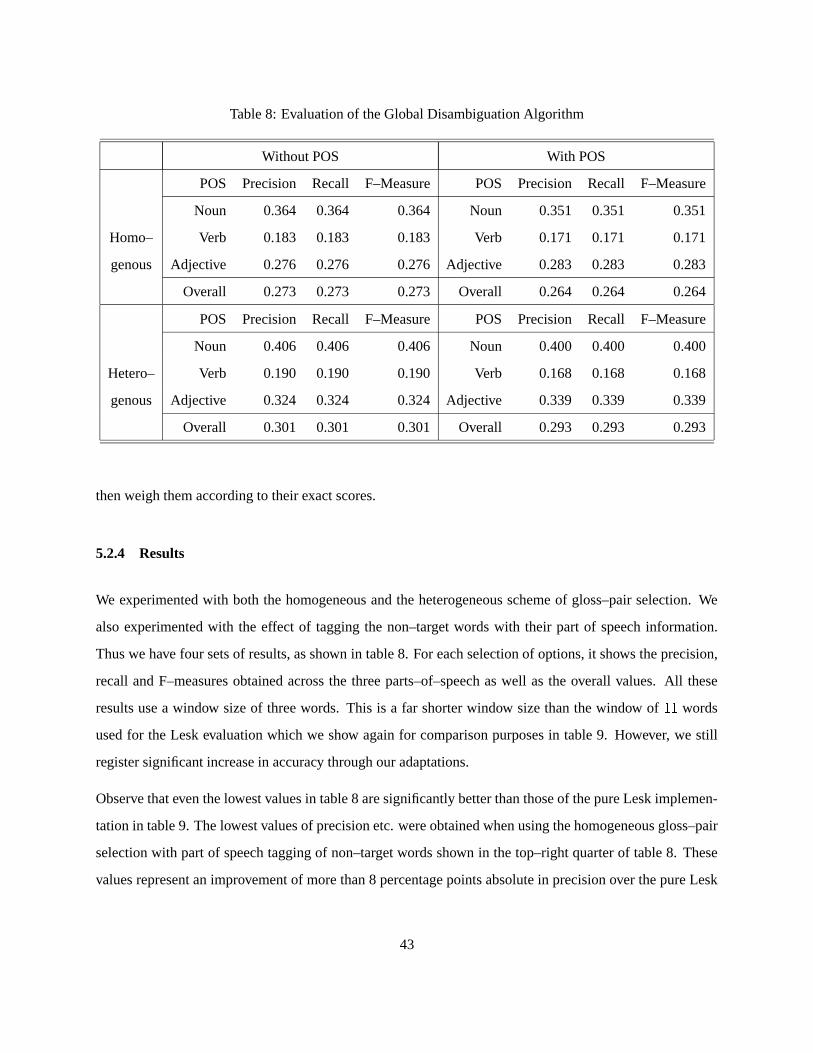
Table 8: Evaluation of the Global Disambiguation Algorithm

Without POS With POS

POS Precision Recall F–Measure POS Precision Recall F–Measure

Noun 0.364 0.364 0.364 Noun 0.351 0.351 0.351

Homo– Verb 0.183 0.183 0.183 Verb 0.171 0.171 0.171

genous Adjective 0.276 0.276 0.276 Adjective 0.283 0.283 0.283

Overall 0.273 0.273 0.273 Overall 0.264 0.264 0.264

POS Precision Recall F–Measure POS Precision Recall F–Measure

Noun 0.406 0.406 0.406 Noun 0.400 0.400 0.400

Hetero– Verb 0.190 0.190 0.190 Verb 0.168 0.168 0.168

genous Adjective 0.324 0.324 0.324 Adjective 0.339 0.339 0.339

Overall 0.301 0.301 0.301 Overall 0.293 0.293 0.293

then weigh them according to their exact scores.

5.2.4 Results

We experimented with both the homogeneous and the heterogeneous scheme of gloss–pair selection. We

also experimented with the effect of tagging the non–target words with their part of speech information.

Thus we have four sets of results, as shown in table 8. For each selection of options, it shows the precision,

recall and F–measures obtained across the three parts–of–speech as well as the overall values. All these

results use a window size of three words. This is a far shorter window size than the window of ��� words

used for the Lesk evaluation which we show again for comparison purposes in table 9. However, we still

register significant increase in accuracy through our adaptations.

Observe that even the lowest values in table 8 are significantly better than those of the pure Lesk implemen-

tation in table 9. The lowest values of precision etc. were obtained when using the homogeneous gloss–pair

selection with part of speech tagging of non–target words shown in the top–right quarter of table 8. These

values represent an improvement of more than 8 percentage points absolute in precision over the pure Lesk

43

Table 9: Pure Lesk Evaluation

Part of Speech Precision Recall F–Measure

Noun 0.258 0.258 0.258

Verb 0.116 0.116 0.116

Adjective 0.170 0.170 0.170

Overall 0.183 0.183 0.183

evaluation, which is about a � ��

relative improvement.

The best precision values are obtained for the experiments using the heterogeneous scheme of gloss–pair

selection with a very minor difference between those obtained using the part of speech information of the

non–target words and those not using. Observe from the lower left section of table 8 and from table 9 that

both the nouns and the adjectives register an improvement of close to 15 percentage points while the verbs

show a 8 percentage point increase. These increases translate to an overall increase in precision of close to

12 percentage points which is a relative improvement of nearly 67%.

These are very encouraging results when compared to our benchmark Lesk evaluations. These results also

represent a marked improvement over the near Lesk results presented at SENSEVAL–2. Two variations

of the Lesk algorithm were presented at this venue. The first counted the number of words in common

between the instance in which the target word occurs and its gloss. Each word count was weighted by its

inverse document frequency which was defined simply as the inverse of the number of times the word has

occurred in the instance or the gloss in which the word occurs. The gloss with the highest number of words

in common with the instance in which the target word occurs represents the sense assigned to the target

word. This approach achieved overall recall of 16 %.

A second approach proceeded identically, except that it added example texts that WordNet provides to

the glosses. This achieved recall of 23%. This suggests that the example strings associated with the various

synsets are a potential source of useful information. We make use of them in our later algorithms (see section

7). However, since our baseline approach does not use example texts, the most indicative comparison is with

the approach that does not use the example strings. By including an extended notion of which glosses to

compare a target word’s gloss with and by using a modified scoring scheme, our baseline algorithm improves

44

precision from 16% to 30%, which is a relative improvement of 87%.

In addition, this baseline approach compares favourably with other systems entered in SENSEVAL-2. Of

the seven unsupervised systems that did not use any of the available training examples and only processed

test data, the highest ranked achieved recall of 40%, and this was one of only two systems that achieved

more than 30% recall.

It is encouraging to note that our algorithm shows such a considerable amount of improvement over the

classic Lesk approach by the simple mechanism of augmenting the glosses of the words being disambiguated

with the glosses of other words associated with them. However we believe that depending upon the data, the

global disambiguation mechanism can be unnecessarily computationally intense. Recall that it computes

scores for every combination of senses in the window of context words. This can be very useful in a setting

where we know that the words in the window are indeed highly related to each other. This is true for short

queries in the realm of information retrieval where accurate disambiguation can help results and all the terms

in the query can be assumed to be related.

However the SENSEVAL–2 English lexical sample data consists of long sentences in which only a few

words are related to the target word. In such a situation we are unsure if we derive any real benefit from

performing the multitudes of comparisons between words that are often not related to each other at all.

Moreover, such comparisons can lead to spurious matches that can only mislead the disambiguation algo-

rithm. In the next section we propose to ignore all non–target comparisons, and observe the resulting change

in precision, recall and f–measure.

45

6 Local Disambiguation with Heterogeneous Synset Selection

In the previous section we discussed the implementation, evaluation, and drawbacks of the global disam-

biguation algorithm using the glosses of the synsets that the words in the context window belong to, as well

as those of synsets related to them through certain relationships. We observed that while the algorithm does

indeed perform better than the basic Lesk algorithm, it is more suited to situations where all the words in the

context window around the target word are closely related to each other – for example in queries submitted

to information retrieval systems. On the other hand, in text that consists of long sentences, only a few words

may be related to the target word, and the large number of comparisons performed by the global method

are probably redundant. In this section, we ignore all comparisons between non–target words and show that

when tested on the English lexical sample data of SENSEVAL–2, there is no appreciable loss of precision,

recall and f–measure.

6.1 The Local Disambiguation Strategy

Given a window of�

words, each with some number of senses defined in WordNet, the global disambigua-

tion strategy discussed in the previous chapter compares every sense of a word with every sense of every

other word in the context window. This algorithm works well when the context words are strongly related

to each other and there are chances of detecting relationships between the non–target words.

However, in situations where two words of the context window are clearly unrelated to each other, all

the comparisons involving them are redundant and potentially misleading. We hypothesize that in text

consisting of complete sentences, most words are actually unrelated to the target word and comparisons

between non–target words are therefore often not pertinent to the disambiguation of the target word. We test

this hypothesis by dropping all the comparisons between non–target words. We call this the local approach

to disambiguation as opposed to the global approach of the previous section. Further, for the purpose

of selecting synsets for gloss–comparison, we use the heterogeneous scheme which performed marginally

better than the homogeneous scheme (table 8).

Unlike the global approach where each combination of senses for the words in the window is scored, in this

approach we obtain scores for each sense of the target word. Given a particular sense of the target word,

we compare its gloss and the glosses of synsets related to it through the various relations in table 6 with

46

the glosses of all the senses of all the non–target words in the context window as well as the glosses of

other synsets related to them through the relations in table 6. In each such comparison overlaps are detected

and their normalized squared scores are computed using the scoring mechanism discussed in section 5.1.5.

These scores are all added together to obtain the score for this sense of the target word. Similarly, scores

are computed for the other senses of the target word, and the highest scoring sense is declared as the most

appropriate one.

For example, consider once again the example of section 5.1.6 where we had a window of three words

sentence, bench and offender, where bench is the target word. Further assume that we are interested only

in the hypernym and hyponym relations. Recall that sentence has two senses denoted by sentence#n#1 and

sentence#n#2, bench has two senses denoted by bench#n#1 and bench#n#2 and offender only one sense

denoted by offender#n#1. Following are the glosses of these synsets:

gloss(sentence#n#1) = a string of words satisfying the grammatical rules

of a language

gloss(sentence#n#2) = a final judgment of guilty in a criminal cases and

the punishment that is imposed

gloss(bench#n#1) = a long seat for more than one person

gloss(bench#n#2) = persons who hear cases in a court of law

gloss(offender#n#1) = a person who transgresses law

In the local approach, we obtain a score each for the two senses of the target word bench. Figure 7 shows the

comparisons done for bench#n#2. Observe that we compare gloss(bench#n#1) with gloss(sentence#n#1),

gloss(hype(sentence#n#1)), gloss(hypo(sentence#n#1)), gloss(sentence#n#2), gloss(hype(sentence#n#2)),

gloss(hypo(sentence#n#2)), gloss(offender#n#1), gloss(hype(offender#n#1)) and gloss(hypo(offender#n#1)).

Similarly, gloss(hype(bench#n#1)) is compared with all these glosses. Note that bench#n#1 has no hy-

ponym, and so comparisons involving the hyponym of bench#n#1 cannot be done. In all these comparisons,

overlaps are detected and scored using the mechanism outlined in section 5.1.5. Table 10 shows the scores

from each comparison and the resulting overall score for this sense of bench.

Similarly comparisons are performed and a score is computed for bench#n#1. That sense that gets the higher

score is declared as the most appropriate one for the target word bench.

47

who hear

who transgresses

{administration, governance, establishment}who make up a governing body

and who administer something"persons"the

hype(bench#n#2){bench, judiciary}

"persons cases in acourt of law"

bench#n#2

{rape conviction}, {robbery conviction}"conviction for murder; conviction for rape

{murder conviction}

conviction for robbery"

"a string of words satisfying the{sentence}

rules of grammar"

{sentence, conviction, judgement of conviction}

the punishment that is imposed""the final judgment of guilty in criminal cases and

a sentence composed of at least one main clause{complex sentence}, {compound sentence}

at least two coordinate independant clausesand one subordinate clause; a sentence composed of

hypo(sentence#n#1)

{bad person}who does harm to

others"person"a

{convict}, {felon}{attacker},

commits a crime"of a criminal offence; someone who

"someone who attacks; person convicted

{string, string of words}a linear sequence of words as

spoken or written

hype(sentence#n#1)

{final judgement, final decision}

before the court of law""a judgement disposing of the case

hype(sentence#n#2)

{wrongdoer, offender}law""person

offender#n#1

hypo(sentence#n#2)

sentence#n#1 sentence#n#2

hype(offender#n#1)hypo(offender#n#1)

Figure 7: The comparisons done in the local approach for bench#n#2. Ovals show synsets, with synset

members in���

and the gloss in quotation marks. Dotted lines represent the various gloss–gloss comparisons.

Overlaps are shown in bold.

48

Table 10: Computation of the Score for the Combination in Fig. 7

First Gloss Second Gloss Overlap String Normalized Score

hype(bench#n#2) hype(offender#n#1) person 0.015

hype(bench#n#2 offender#n#1 person 0.022

hype(bench#n#2) hypo(offender#n#1) person 0.006

bench#n#2 hype(sentence#n#2) court of law, case 0.111

bench#n#2 sentence#n#2 cases 0.008

bench#n#2 hype(offender#n#1) person 0.018

bench#n#2 offender#n#1 person, law 0.055

bench#n#2 hypo(offender#n#1) person 0.097

Total score for sentence#n#2 – bench#n#2 – offender#n#1 0.332

Observe that unlike in the global approach, comparisons are never made between the non–target words. Thus

we never compare the glosses associated with sentence with the glosses associated with offender. While this

is intended to avoid comparisons between completely unrelated words, observe that this also reduces the

time complexity of the algorithm. In more formal terms, assume that on average there are � senses per word

in the context window. Given a window with�

words (of which one is the target word), then there are

���� �� � � (2)

pairs of sets of synsets to be compared. The value of this formula increases linearly with�

, and that makes

this a fairly non–intensive algorithm. Recall from equation 1 that this is unlike the global mechanism in

which the number of pairs of synsets being compared rises polynomially with the value of�

.

We hope to evaluate this algorithm to see if there is an appreciable drop in accuracy from the global approach

of the previous section.

49

6.2 Evaluation of The Modified Algorithm

We have evaluated the local disambiguation algorithm on the SENSEVAL-2 lexical sample data. We first

discuss below the various ways we pre–process the lexical sample data. We follow that by presenting the

results of the evaluation, and conclude with an analysis of the results.

6.2.1 Preprocessing of the Data and Other Issues

Recall that the English lexical sample data is split into instances where each instance consists of a single

target word surrounded by a fairly large number of words that provide the context for the target word.

As in the previous section, we pre–process the contextual data by first identifying compound words. Recall

that compound words are sequences of two or more words that are treated by WordNet at par with single

words or lexemes. As mentioned previously, these may be proper nouns like New York City or phrases

like pull the leg of. Also recall that by identifying and using compounds instead of their individual words

separately, we hope to improve accuracy of the disambiguation algorithm.

Unlike the previous section, we do not tag the non–target words with their part of speech information. Recall

our observation in the previous section that the part of speech tagging of the non–target words does not seem

to affect the accuracy of the system much, and so we elect to avoid the tagging step. Thus when considering

the senses of a particular non–target word, we consider all its senses across its various possible parts of

speech. We do however continue to use the part of speech of the target word because this information

is already provided to us by the organizers of SENSEVAL–2 and is also highly accurate since it is not

obtained through automatic means.

As before, we compare two strings only after performing morphological stemming on the words contained

therein, by which inflected words are replaced by their base forms as defined by WordNet. Recall that this

ensures we do not miss words like cat and cats when matching two strings.

Recall that in the global method, we could only experiment with context windows that were three words

long. The much reduced computational complexity of the local method offers us the luxury of choosing

longer windows of context and thereby observing the effect of a growing window on the precision and recall

of the disambiguation process. In particular, we run the same algorithm with window sizes 3, 5, 7, 9, and

50

Table 11: Relations Chosen For the Disambiguation Algorithm

Noun Verb Adjective

Hypernym Hypernym Attribute

Hyponym Troponym Also see

Holonym Also see Similar to

Meronym Pertainym of

Attribute

11. We use odd numbered window sizes so that we can select an equal number of words to the left and the

right of the target word. Note however, that if the target word itself is too close to the start or the end of the

instance, then an equivalent number of words are selected from the other direction. In selecting the context

window, we once again avoid words that do not belong to any synset in WordNet. Further, when selecting

the candidate senses of each word in the context window, we select only those senses of the target word that

are consistent with its given part of speech and all the senses of the non–target words since we are neither

given nor do we compute their parts of speech for this set of experiments.

Table 11 shows the relations used to select synsets whose glosses will be compared. Observe that this is

exactly the same as the relations used in the previous section (table 6). Further, we use the heterogeneous

scheme of gloss comparison. Recall that in this method, given two synsets for comparison, every synset

related to the first one is compared to every synset related to the second one. We have shown in the previous

section that the homogeneous scheme of synset selection, in which the glosses of only those synsets that are

related to the synsets of the context words by the same relationship are compared, performs disambiguation

at a slightly lower accuracy as compared to the heterogeneous scheme. Henceforth therefore, we elect to

use the heterogeneous scheme.

As in the previous section, we continue to detect multi–word overlaps between the glosses being compared,

as opposed to the original Lesk algorithm of just counting the number of words matched. Further, we

continue to give a higher weight to multi–token overlaps by squaring the number of tokens in an overlap.

51

6.2.2 Results

Results in table 12 and fig. 8 represent the precision, recall and f–measure values obtained by using the local

disambiguation approach with the heterogeneous gloss–pair selection scheme for window sizes 3, 5, 7, 9,

and 11. The maximum overall precision of 3.24% is achieved for a window size of 11. This value represents

an increase of more than 2% absolute and 7.6% relative when compared to the global heterogeneous scheme

with a window size of 3 (table 8). This also represents an improvement of 14 percentage points over the

pure Lesk implementation which represents an improvement of 72% relative.

Precision on the nouns and the verbs improved by more than 2 and 3 percentage points respectively. We

hypothesize that this is partly due to the extra information available to the system from the larger windows

of context. Precision on the adjectives rose by a more modest 1 percentage point.

Overall, the precision and recall values seem to peak around a window size of , that is when the context

window includes the target word, four words to the left of the target word, and four words to the right. These

values begin to fall away gradually beyond this window size, which seems to suggest that words that are

distant from the target word may not help the disambiguation process much but instead might serve to add

extra and perhaps misleading information.

6.3 Analysis of Results

We continued to follow the same techniques in reporting answers that were introduced in the previous

section. Thus, target words with scores of 0 for all their possible senses were left untagged, and when

multiple senses were tied at the highest score, all of them were reported. Also, as mentioned previously, we

used the same relations as we did for the previous iteration; these are listed in table 11.

We observe from these experiments that on the data we have used for evaluation the local method not only

disambiguates faster, but also more accurately than the global method. As mentioned above, we believe

that this higher accuracy can be attributed to the fact that the global approach often performs comparisons

that are unnecessary, and worse, misleading. By avoiding comparisons between glosses associated with the

non–target words, this problem is mitigated to some extent.

Further, the limited computational intensity of the local method affords us the luxury of employing larger

52

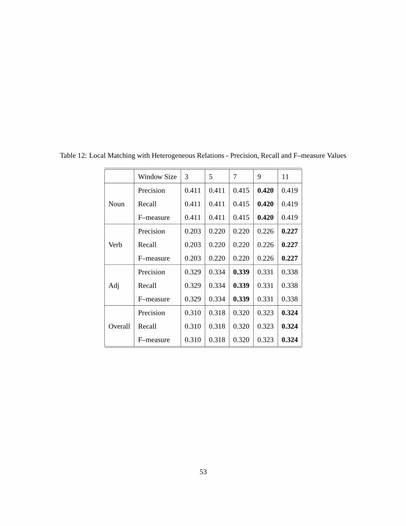
Table 12: Local Matching with Heterogeneous Relations - Precision, Recall and F–measure Values

Window Size 3 5 7 9 11

Precision 0.411 0.411 0.415 0.420 0.419

Noun Recall 0.411 0.411 0.415 0.420 0.419

F–measure 0.411 0.411 0.415 0.420 0.419

Precision 0.203 0.220 0.220 0.226 0.227

Verb Recall 0.203 0.220 0.220 0.226 0.227

F–measure 0.203 0.220 0.220 0.226 0.227

Precision 0.329 0.334 0.339 0.331 0.338

Adj Recall 0.329 0.334 0.339 0.331 0.338

F–measure 0.329 0.334 0.339 0.331 0.338

Precision 0.310 0.318 0.320 0.323 0.324

Overall Recall 0.310 0.318 0.320 0.323 0.324

F–measure 0.310 0.318 0.320 0.323 0.324

53

0

0.2

0.4

0.6

0.8

1

3 4 5 6 7 8 9 10 11

Pre

cis

ion

pe

rce

nta

ge

Window size

NounsVerbs

AdjectivesOverall

0

0.2

0.4

0.6

0.8

1

3 4 5 6 7 8 9 10 11

Re

ca

ll p

erc

en

tag

e

Window size

NounsVerbs

AdjectivesOverall

0

0.2

0.4

0.6

0.8

1

3 4 5 6 7 8 9 10 11

Fm

ea

su

re p

erc

en

tag

e

Window size

NounsVerbs

AdjectivesOverall

Figure 8: Local Matching Approach with Heterogeneous Relations - Precision and Recall

54

windows of words around the target word. Indeed we observe that a window size of around 9 words centered

around the target word appears to help achieve the best accuracy figures. We also note that longer windows

fail to do equally well, presumably because words that are that far away from the target word are not related

enough to it, and merely add noise to the process.

Another interesting observation is that the nouns continue to outperform the verbs and adjectives by quite

a margin. We believe that this difference can be attributed to the fact that in WordNet verbs are inherently

more polysemous and subject to much finer sense distinctions that nouns. In fact, the particular verbs used

in SENSEVAL-2 have on average close to three times the number of senses that the nouns have, as shown

in table 3. This makes disambiguation decisions even harder to make for verbs as compared to nouns and

adjectives.

We believe two factors combine to produce the happy results above. First, recall that the results above

are based on much longer context windows than we could use for the global algorithm in the previous

chapter. Such long windows provide greater numbers of overlapped tokens and, as it turns out, more accurate

information than the much shorter 3–word window experimented with in the previous section. A larger

window however can also introduce a larger amount of noise. Fortunately however, it appears that the useful

information more than balances out the noise up to a window size of 9. However after a point it seems that

the noise does indeed exceed the useful information, and accuracy once again drops.

Another factor that may partially explain the good results above is that we are no longer performing the

multitudes of comparisons done for the global method. In the local method experimented with here, no

comparisons are performed between non–target words. While this may deny us some pieces of useful

information that may help the disambiguation, we believe that much greater benefit is drawn from the

reduced noise that results from cutting out comparisons between non–target words.

Through the modifications in this iteration we have successfully proved our hypothesis that the large num-

bers of comparisons between the non–target words performed by the global approach of the previous section

are seldom warranted, particularly on the kind of data we are evaluating our algorithms on. In fact, we have

shown that we can achieve even greater accuracy by taking on a larger window of context, and have shown

that a window of 9 words appears to result in maximum disambiguation accuracy.

Our overall f–measure value of 32.4% ranks third when compared against the results achieved by the par-

55

ticipants of the SENSEVAL–2 exercise (table 5). Only two teams score higher than our current system on

f–measure. Observe that our results have been obtained by solely utilizing the glosses of various synsets.

Recall however that WordNet stores for each word several other pieces of information besides its defini-

tional gloss such as synonyms and example sentences. We propose to utilize these strings of words as well

as the context in which the word occurs itself to try and detect overlaps, and to observe whether this has any

positive effect on the accuracy of disambiguation.

56

7 Augmenting the Algorithm with Non–Gloss Information

In the previous sections we have proposed, implemented and evaluated a set of modifications to the basic

Lesk word sense disambiguation algorithm. We have shown that our adapted algorithm performs much

better than the original Lesk algorithm, and reasonably well when compared against the performances of the

participants of the SENSEVAL–2 word sense disambiguation exercise.

However, we have also noted that thus far we have utilized only the glosses of the various synsets for

comparisons. WordNet stores several other pieces of information for each synset. For example, many

synsets have more than one word or synonym in them that can also be used to represent the same concept –

we have not made use of these synonyms so far. Further many synsets have example sentences that illustrate

typical uses of the words in the synset. Although these sentences vary widely in length and quality, recall

that by using them it was possible to improve the accuracy of the baseline Lesk algorithm from �� ��� to ������

in the SENSEVAL–2 competition. Finally, for each target word in our test data, recall that we are provided

with a context of two to three preceding sentences. After selecting the words that form the short window of

context around the target word, we have thus far ignored the rest of the context string. We propose to use

this too in our experiments below.

7.1 Using Extended Information

7.1.1 Overlaps Resulting from Synonym Usage

In coherent speech and writing, human beings often talk of related topics. Further, when expressing the

same idea multiple number of times, they are encouraged to use a different synonym each time. Recall that

in WordNet, a synset is a group of synonyms that can be used somewhat interchangeably to mean the same

thing. Further recall that along with each target word in the SENSEVAL-2 test data, we are provided with

one or two preceding and succeeding sentences that we call the context of the target word. We hypothesize

that if we find a word in this context such that one of its senses belongs to the same synset as a certain sense

of the target word, then that provides very high evidence in favour of that particular sense of the target word.

Consider for example the context made up of the following pair of consecutive sentences: He has a great

figure. He works very hard to maintain his physique. Assume figure is the target word. Notice that the

57

word physique occurs further down the next sentence. Both the words figure and physique occur in a synset

that means alternative names for the body of a human being, and this is very strong

evidence that this is indeed the intended sense of the word figure above. Similarly, in the sentence He made

a name for himself in the world of literature, and is now an important figure, the fact that the words figure

and name occur in the same synset with meaning a well-known or notable person is almost convincing

evidence in favour of this sense of the word figure.

Observe of course that with a suitably large window size, we would be able to detect such synonyms through

our gloss–gloss comparisons as well. However we have seen that such large window sizes are impractical,

and so we do a direct search between the other words in the synsets of the target word and the context string.

Note however that even if we do detect a synonym of the target word being used elsewhere in the context

string, such an overlap will have a length of only one. Obviously this match deserves a much stronger score.

In particular, if the synonym was in the selected small window of words around the target word, then its

own gloss and the glosses of all synsets related to it would have matched completely with the gloss and the

related glosses of that sense of the target word it shares a synset with. So one approach could be to add up

the scores of all such overlaps and use this sum as the score for this particular match between the synset and

the context.

In practice though, we would like to give it a slightly lower score to penalize for the fact that the word is

not in the immediate vicinity of the target word. This is in keeping with our hypothesis that words that

are closest to the target word are most indicative of its sense, and words located further away are less so.

Hence, we divide the score computed above by the number of words that lie between the target word and its

synonym in the context string.

Thus in our He has a great figure. He works very hard to maintain his physique example above, assuming

we are using the glosses of the synsets themselves and the glosses of their hypernyms and hyponyms, we

first compute the sum of all possible overlaps between these glosses for the senses of the words figure

and physique that share a synset. The gloss of the synset�figure, physique

�is alternative names

for the body of a human being leading to a score of 81; the gloss of the hypernym of the synset�figure, physique

�is the entire physical structure of an organism which contributes a

score of 36 (recall that we drop the function word the from the overlap); and the gloss of the hyponym of�figure, physique

�is a person’s body usually including their clothing which gives

58

us a score of 36. Adding these up, we get a score of 153. Finally since physique is 8 words away from

figure, we divide this number by 8 to arrive at 19 as the score for this synset–context overlap.

7.1.2 Overlaps Resulting from Topically Related Words

Although words in WordNet are organized into IS–A, IS–A–Kind–Of, etc. hierarchies, there are no links

between words that are only topically related to each other. Thus for example, the synset�wave

�that means

one of a series of ridges that moves across the surface of a liquid

especially across a large body of water is not connected directly to the synset�body

of water, water�

which means the part of the earth’s surface covered with water

through any of the relations defined in WordNet. Further observe that the only word that overlaps be-

tween their glosses is water, which is also an overlap between the sense of�wave

�above and the sense

of�water supply

�which means facility that provides a source of water. Clearly, the

synset�body of water, water

�is more closely related to

�wave

�, and indeed this can be observed by com-

paring the synset member body of water to the gloss of the synset�wave

�.

In general when two words are topically related, we can hope to find in the gloss of one of the words

synonyms of the other word. Thus in our example above, if the words wave and water were used in the same

sentence, by looking for matches between the gloss of wave and the synset members of water we would find

a 3 word match.

Similarly, given two words that are topically related, we can hope that the example strings of one of the words

may use synonyms of the other word. For example, say we have the words interest and mortgage. The related

senses of these two words incidentally have no overlaps between them, and neither are they related through

any of the WordNet relations. However, the example string of the appropriate sense of interest is: how

much interest do you pay on your mortgage?. The occurrence of the word mortgage here

can help us spot the relationship between these two senses.

We could find overlaps between the example strings of topically related words too, and so we shall perform

comparisons between the examples strings of synsets.

59

Table 13: List of Extended Data Used for Comparisons

synset members – context

synset members – gloss

synset members – example

context – example

context – gloss

example – example

example – gloss

7.1.3 Other Possible Sources of Overlaps

Sometimes words are used in a definitional way, that is in a sentence that basically explains the meaning

of the word. For example the preceding sentence defines what definitional writing is, and uses the words

explain, meaning and word all of which are in the gloss of the word definition: a concise expla-

nation of the meaning of a word or phrase or symbol. We propose to compare the

context of the target word with its gloss to detect such cases.

Table 13 lists the comparisons made for this round of experiments. Note that there are some comparisons

we want to avoid. For instance we wish to avoid comparing two synsets for overlaps. This is because if we

indeed find a word that is common to the two synsets, then that word is being used in two different senses

in those synsets, and the overlap could actually be an indication of the fact that these two synsets are not

related to each.

7.2 Evaluation of the Augmented Algorithm

We evaluate the algorithm with the extended information on the English lexical sample data. In the next

section we discuss some of the preprocessing steps done on the data, and then present the results.

60

7.2.1 Preprocessing and Other Details

We perform for this set of experiments exactly the same preprocessing steps as in the previous section.

Thus compound words are identified and words in strings are stemmed before attempting to match them.

Continuing from the previous section, we do not tag the non–target words with their parts of speech, and

therefore consider all possible senses across all possible parts of speech for them. On the other hand we do

use the part of speech already provided to us for the target word and consider only those of its senses that

are consistent with its given part of speech.

As in the previous section, we use the local disambiguation strategy which we have shown to be highly

successful on the kind of data contained in the English lexical sample. Recall that in this approach, we

score each sense of the target word by comparing the information associated with it with all the information

associated with all the senses of all the other words in the context window. Further, we utilize window sizes

of 3, 5, 7, 9 and 11.

Note that we utilize in our algorithm two sets of data. First we perform all the combinations shown in

table 13. Second, we also perform all the comparisons performed in the previous section. Thus we do

a completely heterogeneous comparison between the relations in table 11. Recall that in heterogeneous

comparisons, the gloss of every synset related to one of the synsets of a context word is compared with

the gloss of every synset related to one of the synsets of another context word. Thus we have a total of 91

possible comparisons.

To score senses, we continue to look for multi–word overlaps, and compute scores for comparisons by

squaring the lengths of these multi–word overlaps.

7.2.2 Results

Results in table 14 and figure 9 show the precision, recall and f–measure values achieved by augmenting the

glosses used up to the previous section with some other information stored in WordNet. The highest overall

precision is recorded at around ��� ����� which is 1 percentage point higher than the highest in the previous

section.

Precision on all three parts of speech improve by between 1 and 3 percentage points each. The overall

61

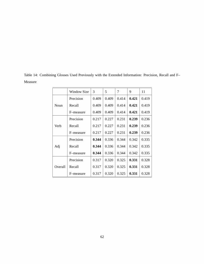
Table 14: Combining Glosses Used Previously with the Extended Information: Precision, Recall and F–

Measure

Window Size 3 5 7 9 11

Precision 0.409 0.409 0.414 0.421 0.419

Noun Recall 0.409 0.409 0.414 0.421 0.419

F–measure 0.409 0.409 0.414 0.421 0.419

Precision 0.217 0.227 0.231 0.239 0.236

Verb Recall 0.217 0.227 0.231 0.239 0.236

F–measure 0.217 0.227 0.231 0.239 0.236

Precision 0.344 0.336 0.344 0.342 0.335

Adj Recall 0.344 0.336 0.344 0.342 0.335

F–measure 0.344 0.336 0.344 0.342 0.335

Precision 0.317 0.320 0.325 0.331 0.328

Overall Recall 0.317 0.320 0.325 0.331 0.328

F–measure 0.317 0.320 0.325 0.331 0.328

62

highest recall and f–measure values are obtained once again at a window size of 9. Nouns and verbs both

perform best at a window of size 9 whereas the adjectives curiously do best at the smallest window size. We

are unsure why such should be the case.

0

0.2

0.4

0.6

0.8

1

3 4 5 6 7 8 9 10 11

Pre

cis

ion

pe

rce

nta

ge

Window size

NounsVerbs

AdjectivesOverall

0

0.2

0.4

0.6

0.8

1

3 4 5 6 7 8 9 10 11R

eca

ll p

erc

en

tag

e

Window size

NounsVerbs

AdjectivesOverall

0

0.2

0.4

0.6

0.8

1

3 4 5 6 7 8 9 10 11

Fm

ea

su

re p

erc

en

tag

e

Window size

NounsVerbs

AdjectivesOverall

Figure 9: Local Matching Approach with Extended Information – Precision, Recall and F–measure

7.3 Analysis of Results

As with the previous chapters target words are left untagged if every one of their senses get a score of 0,

and if multiple senses are tied at the same highest score, they are all reported. We observe that by utilizing

63

the example strings and the synonyms of the target words, we register a modest improvement in precision,

recall and f–measure. Further, the extra comparisons do not adversely affect the speed of computation.

As in the previous section, we get the highest precision values at a window size of 9. Beyond a window size

of 9 words, the precision and recall values taper off implying perhaps that longer windows do not necessarily

result in better results.

As before, the nouns continue to perform better than the other two parts of speech. However the added

information does not seem to have a major effect on the performance of the nouns and adjectives. This leads

us to believe that perhaps with the current formulation of the algorithm, performance of these two parts of

speech has begun to asymptote, and considerable further improvement in results will require much richer

sets of information. One possible source of such information could be to utilize synsets that are more than

on hop away from the synset that the target word belongs to. Recall that at present we utilize only synsets

that are directly connected to the synsets of the words in the window of context, and none that are indirectly

connected via a third synset. We hypothesize that only a huge increase in the information provided to the

algorithm will result in a big improvement in results, at least for the nouns and adjectives.

The less moderate improvement in performance for the verbs suggests that while performance on the nouns

and adjectives may have started to asymptote, the verbs continue to benefit from added pieces of information

and are yet to reach a ceiling in terms of performance.

Our overall f–measure value of 33.1% continues to rank third as compared to the results achieved by the

participants of the SENSEVAL–2 exercise (table 5). On the other hand our recall value ranks second when

compared to other SENSEVAL–2 systems.

64

8 Conclusions

In this thesis we have adapted Lesk’s algorithm for word sense disambiguation using dictionary definitions

[11] to the electronic lexical database WordNet. Given a target word to be disambiguated and a few sur-

rounding words that provide the context of the word, we have not only used the definitional glosses of these

words, but also those of words related to them through the various relations defined in WordNet. We have

also attempted to use other data stored by WordNet for each word, such as example sentences, synonyms

etc. We have experimented with various schemes of choosing glosses for comparison and have introduced

a novel mechanism to quantitatively express the extent of relationship between two glosses based on the

overlapped words.

In particular we have experimented with the global and the local disambiguation strategies. In the global

strategy, every possible combination of senses for the words in the context window is tested, and the best

combination is reported, thereby simultaneously disambiguating every word in the context window. In the

local strategy on the other hand, the gloss of each sense of the target word is compared at once with the

concatenation of the glosses of all the senses of the non–target words. We have observed that the global

strategy is highly computationally intensive and have been able to experiment with a window size of only

three words. We have hypothesized that it is best suited for situations where we have a group of highly

related words to disambiguate. We have demonstrated that on text made up of long sentences, it actually

performs poorly due to the noise from the large numbers of unnecessary comparisons it does. The local

method on the other hand has been shown to actually perform better than the global method on this kind of

data, although it does far fewer comparisons.

Given the glosses of a large number of related synsets to utilize in the comparisons, we have introduced and

experimented with two different schemes for choosing pairs of glosses to compare. In the heterogeneous

scheme, we compare the gloss of every synset related to the synset of one context word with that of every

synset related to the synset of another context word. In the homogeneous scheme, we compare the glosses

of two synsets only if they are related to the synsets of the context words through the same relation. We have

found that the heterogeneous scheme performs better than the homogeneous scheme by a small margin of

about 1 to 2 percentage absolute.

We have also shown that tagging the non–target words with their part of speech information is unnecessary

65

and have concluded from this that our algorithm is not adversely affected by the absence of part of speech

information of the non–target words. Thus data need not be syntactically parsed before it is disambiguated

by this algorithm.

The local method is computationally cheaper than the global method, and allows us to experiment with

various window sizes. We have experimented with window sizes 3, 5, 7, 9 and 11, and have noticed that

the best precision and recall values are achieved at a window size of 9. Beyond that size, the precision and

recall values start falling again, implying that the extra words added to the context window bring more noise

than useful information to the disambiguating algorithm.

Besides utilizing the glosses of the various synsets, we have also attempted to use other pieces of information

stored by WordNet like example sentences, synonyms of context words and the context in which the target

word appears. We have shown that this information helps improve the disambiguation of verbs much more

than nouns and adjectives.

Although the original Lesk algorithm “scored” two glosses by counting the number of words that overlap

between them, we have introduced a novel scoring scheme where the glosses are thought of as sets of words,

and the overlaps their intersection set. Given this set–up we have applied the dice–coefficient as a test of

association between these two glosses; larger overlaps will imply that the glosses have a stronger association

with each other. Further, we have been motivated by Zipf [18] to seek and weigh more heavily multi–word

overlaps since longer overlaps are exponentially rarer, and therefore deserve an exponentially increasing

weight. Given an overlap that is � tokens long, we have over–counted the tokens in this overlap � times

each. Thus the dice value computed is proportional to the square of the number of tokens in a multi–token

overlap.

We have implemented the original Lesk algorithm and have evaluated it on the English lexical sample

data of SENSEVAL–2. This algorithm achieves an overall f–measure value of ��� ����� . Using the global

disambiguation strategy along with the heterogeneous scheme of gloss–pair selection, we have been able to

improve this to an overall f–measure of ��� � ��� . We have then used the local strategy with the heterogeneous

scheme and have shown that with a window size of 9, we can further improve overall f–measure to �� ��� � .

Finally we have shown that by adding the extended information like the example sentences and synonyms,

f–measure values improve only marginally to ��� � ��� .

66

These values compare favourably with those achieved by the participants of the SENSEVAL–2 competi-

tion. Of the 7 entrants, only one system achieves higher recall than our system and only two higher precision

and f–measure. We conclude that adapting the Lesk algorithm to WordNet even in our relatively straight for-

ward manner can produce an unsupervised word sense disambiguation system that is not only substantially

more accurate that the original Lesk algorithm, but that also compares favourably with other unsupervised

algorithms on the same data.

67

9 Related Work

In this section we review six papers each of which describes research on word sense disambiguation using

WordNet. [5] and [1] represent work that is closest to this thesis. The former shows how one may combat the

combinatorial explosion when trying to simultaneously disambiguate all the words in a window of context

while the latter describes a method to get the best combination of senses for a window of words, but using a

non–Leskian approach.

[17] and [12] show how one may take advantage of the document in which the target word occurs for its

disambiguation. While [17] uses words far away from the target word for the disambiguation of the target

word, [12] reuses the senses previously assigned to other words in the document to guide the disambiguation

of new words in the same document.

Finally, [10] and [13] propose ways of augmenting the unsupervised disambiguation algorithm with some

knowledge derived from small quantities of manually sense–tagged data. Although our algorithm takes a

purely unsupervised approach, we are always interested in combining the strengths of the two approaches in

a bid to achieve better disambiguation without depending entirely on the supervised technique. These two

papers give some ideas of how this may be done.

9.1 Approaches that Simultaneously Disambiguate All Words in the Window

Several approaches to word sense disambiguation using WordNet have been proposed in the past. Of these,

the algorithm described in Lexical Disambiguation using Simulated Annealing [5] by Jim Cowie, Joe

Guthrie and Louise Guthrie is perhaps the most closely related to our algorithms. In this paper the authors

attempt to tackle a problem first posed in [11] – that of what order to follow when disambiguating all the

content words in a sentence.

Recall that when the original Lesk algorithm [11] disambiguates a word in a sentence, it does not make

use of the senses it has assigned to words prior to it in the same sentence. Another possible scheme is

to evaluate all possible combinations of senses for the content words of a given sentence, and to pick that

combination that is deemed the most appropriate. We call this the global scheme of disambiguation, and

have experimented with it in chapter 5. We have shown that indeed this leads to slightly more accurate

68

disambiguation than the method described by Lesk [11] over the same window size. However we have also

shown that due to the combinatorial explosion of candidate sense combinations, this method is too intensive

to be useful for us. This paper attempts to tackle this computationally intensive aspect through the use of an

algorithm called simulated annealing.

This algorithm searches through a huge solution space for that solution that minimizes an error function.

Some algorithms that attempt the same thing suffer from the local minima problem in which they get stuck

at a point in the solution space which has a lower error than all points in its neighbourhood, but whose error

is not the lowest global error. Simulated annealing attempts to reduce the probability of getting stuck in

a local minimum by taking random jumps towards higher error points from lower error points during its

search through the solution space. These jumps are taken more often in the initial stages of the search when

it is more likely for the algorithm to get stuck in a local minimum point, and less often in the later stages

when the algorithm is more likely to be close to the global minimum.

To adapt this algorithm to the problem of word sense disambiguation, one must define both a solution space

and an error function. Given a sentence, this paper defines a configuration of senses in exactly the same

way as we define a candidate combination of senses in chapter 5. Thus given�

words, each configuration

consists of one sense each for each of the those�

words, and is distinct from every other configuration for

the given words. The solution space is made up of all such configurations.

Given a configuration, its error value is computed by first adding up the frequencies of all the words that

occur twice or more in the definitions of the senses that make up the configuration. Say this value is rep-

resented by � . The error value is then equal to �� �� � � � . Observe that if each word just occurs once in

all the definitions, then � is equal to 0, and the value of the error function is 1. Conversely, if lots of words

co-occur among the definitions, then the value of � would be large, leading to a low error value. Thus, by

picking that configuration that has the lowest error value, this algorithm chooses that set of senses that have

the most number of word overlaps among their definitions.

The algorithm starts its search through the solution space with that configuration of senses that contains

the first sense of each of the words in the sentence. This algorithm uses the machine readable version of

the Longman’s Dictionary of Contemporary English (LDOCE) in which the senses of a word are arranged

in roughly descending order of frequency of usage. Given this starting configuration, its error value is

calculated as described above. Next, a second configuration is generated from the current configuration by

69

randomly picking one of the�

words and changing its sense from the one it has in the current configuration

to any one of its other possible senses. The error of this new configuration is computed, and if it is found to

be less than the current configuration, then it is accepted as the new current configuration. On the other hand,

if its error is greater than the current configuration, it can still be chosen as the new configuration with a

probability that decreases over time. This process is repeated as long as new configurations get accepted. If

for several iterations no new configurations get accepted, the algorithm stops, and the current configuration

is reported as the most appropriate combination of senses for the words in the sentence.

The authors evaluate this algorithm on 50 example sentences from LDOCE which were first disambiguated

by hand and then the senses reported by the algorithm compared against these human decided senses. The

authors report an accuracy of ���

. Since our algorithms are evaluated on different data, it is difficult to

compare the accuracy values directly. However, accuracy values close to ����

suggest that this is a good

algorithm. This is expected from our experiments too where we show slightly higher accuracy with the

global mechanism, as opposed to the local mechanism experimented by Lesk [11] and by us in chapters 6

and 7. However, as we argue in chapter 5, it is unclear to us if it is necessary to assess all combinations of

senses, particularly when the set of words being disambiguated do not form a closely related phrase.

Another algorithm that attempts to simultaneously assign senses to all the words in a given set is described

in Word Sense Disambiguation using Conceptual Density [1] by Eneko Agirre and German Rigau. In

this paper, the nouns in a given text are disambiguated by taking advantage of the fact that synonyms in

WordNet are grouped into synonym sets or synsets, and these synsets then form IS–A trees through the

hypernym / hyponym links. This paper concerns itself only with noun synsets which it calls noun concepts.

Since WordNet has several IS–A trees, this paper connects the topmost synsets of all the IS–A trees so that

there is always a path between any two noun synsets or concepts.

To disambiguate a noun � , a context window of nouns centered around � is marked off. For example,

say the size of this window is � ��� � and say the nouns in the window are � � , � � , ..., ��

, � , ����� , ...,

� ����� and � �

�in that order. Given that each of these � ��� � nouns has one or more senses in WordNet,

the goal of this algorithm is to select one sense for each of them such that this chosen set of senses is the

most appropriate among all the candidate sets of senses. Recall that this is very similar to our algorithm in

chapter 5 where we attempt to simultaneously assign senses to all the words in the context window.

To achieve this goal, a measure called Conceptual Density is defined for noun concepts in WordNet. Intu-

70

itively, this measure gives a higher score to that noun concept that contains more senses of the words � �

... � ����� in its sub–hierarchy, where the sub–hierarchy of a noun concept consists of all the synsets that

belong to the IS–A sub–tree rooted at it. Further, this measure is inversely proportional to the size of the

sub–hierarchy under consideration, and hence the preference for concepts that have a higher “density” of

concepts.

To find a suitable set of sense each for the � � � � nouns in the context window, the conceptual density of

each noun concept in WordNet is computed, and that concept that has the highest density is chosen. The

senses for the words � � ... � ����� that lie in the sub–hierarchy of this winning concept are assigned to the

words, and thus they are disambiguated. However, only the sense assigned to � is retained, and the rest are

discarded. To disambiguate word ����� for example, this whole process is repeated starting from selecting

the context window.

It is possible that no sense or multiple senses of � are found in the sub–hierarchy of the concept with the

highest conceptual density. In this case, no answer is reported.

The authors test their algorithm on four random files from SemCor [14] which is a collection of data where

every content word is hand–tagged with its most appropriate sense as decided by a human tagger. The sense

definitions used to sense tag the SemCor data are taken from WordNet. The authors report an accuracy of

43% when disambiguating only the polysemous nouns. Assigning senses to monosemous words is trivial,

and when these nouns are also included in the accuracy values, an overall accuracy of 71% is reported.

As mentioned previously, the most striking similarity between this algorithm and ours is that both algorithms

seek to find the best combination of senses for all the words in the context window as opposed to selecting

an appropriate sense for the target word without regard to the appropriate senses of the other words in the

window. However note that it doesn’t really make use of the senses it assigned to the other words and

thereby diverges from our algorithm.

Also, this algorithm works only with nouns. According to the authors, one requires relations that link

together the other parts of speech with nouns for this algorithm to be extended to those parts of speech.

However, such relations are very few in WordNet 1.7.

71

9.2 Approaches that Take Advantage of the Document in which the Target Word Occurs

Although we do evaluate our algorithms on the all–words data which is organized in the form of long

documents, we do not make use of the fact that the sense of a word is strongly influenced by the document

in which it occurs. We review here two papers that may provide guidance on how this may be done.

Using WordNet to Disambiguate Word Senses for Text Retrieval [17] by Ellen M. Voorhees describes an

algorithm that finds the most appropriate sense for the nouns in a document that is part of a larger collection

to aid in information retrieval. Although the algorithm is geared towards a typical information retrieval set–

up and assumes the presence of a document that is a part of a larger group of related documents, the basic

disambiguation algorithm is general enough to be applied anywhere. Further we are interested in the way

in which words that are far from the target word but belong to the same document are incorporated into the

disambiguation algorithm.

Like the previous algorithms, this algorithm too makes use of the IS–A tree among nouns as defined through

the hypernym / hyponym links and attempts to find the largest set of synsets that are all related to a single

sense of a given noun and not related to any other sense of that noun. Specifically, it defines a hood of a sense

� of a polysemous noun to be “the largest connected subgraph that contains � , contains only descendants of

an ancestor of � , and contains no synset that has a descendent that includes another instance of a member

of � as a member”. Intuitively, given a synset � , one traverses up the IS–A hierarchy and stops just before

the first synset which includes as a descendant a synset that has at least one word in common with � . To

disambiguate a given noun, the hood of each of its senses is identified, the number of nouns in the source

text that occur in each hood is counted and the hood with the highest count is selected as the winning hood.

The sense of the noun in the winning hood is assigned to it.

Although the disambiguation of nouns through this algorithm does not in general improve the precision

and recall of document retrieval, the author suggests that this is perhaps due to the fact that it is difficult

to accurately disambiguate words in a very short query. It will be interesting to see how accurate the

disambiguation algorithm is when used in a stand–alone manner.

In the meanwhile, this algorithm represents one way to incorporate the context of a document, or the dis-

course context, while disambiguating a word. In the context of the SENSEVAL all–words data which is

organized into three long documents, this method could be one way to augment our algorithm. Recall that

72

we already attempt to match the synset members of synsets that the target word occurs in as well as the

gloss and example strings associated with the target word against the context that the target word appears in.

Using this paper’s idea, one possible extension to this kind of matching could be to not only use the synsets

associated with the target word, but to also find the hood of the senses of the target word and to then find the

number of words in the context that appear under this hood. Such an extended matching may lead to better

disambiguation of the target word.

Another algorithm that attempts to take advantage of a large document is A WordNet–based Algorithm for

Word Sense Disambiguation [12] by Xiaobin Li, Stan Szpakowicz, Stan Matwin. This paper describes an

algorithm that disambiguates noun–objects of verbs. For example, given the verb, noun–object pair (water,

plants) from the sentence water the plants, it tries to disambiguate the noun plant in its verb–context

water. That is, given that a noun ��

is the object of a verb ��� , this algorithm attempts to choose the

appropriate sense for ��

from the�

possible senses of ��

as defined in WordNet. Thus this algorithm

disambiguates ��

given a ( ��� , ��

) pair. At several points in the algorithm, previously disambiguated

verb–noun object pairs are utilized to disambiguate new pairs.

The algorithm bases its disambiguation decisions on the semantic similarity of words. This similarity is

measured by utilizing the IS–A relationships defined between synsets in WordNet. Two words�

and � are

said to be most similar when they are synonymous, that is when some sense of�

is in the same synset as

some sense of � . Word�

is called an extended synonym of word � if some sense of�

belongs to a synset

that is the hypernym of the synset that some sense of word � belongs to. Word�

is considered hyponymous

with word � when some sense of�

is in a synset that is the hyponym of the synset that some sense of �

belongs to. Finally�

is said to have a coordinate relationship with � if some sense of�

and some sense of

� belong to synsets that have a common hypernym.

Given a verb–noun object pair ( ��� , ��

) where word ��

has to be disambiguated, this algorithm proceeds

by testing eight conditions with respect to ��

in a fixed order, and stopping at the first test that yields a

sense for ��

. Each test also results in a confidence level which decreases monotonically from test 1 to test

6.

The first test checks if ��

has only one sense in WordNet; in this case this is the appropriate sense for ��

and the confidence level is 1.0. If this is not the case, that is, if ��

has more than one sense in WordNet, then

the algorithm looks for another verb–noun object pair ( ��� , ��

�) where �

�

�is synonymous or hyponymous

73

with a sense � of ��

. Sense � is then the appropriate sense of ��

with a confidence level of 0.9. If such a

( ��� , ��

�) pair cannot be found, and instead another pair ( ��� , �

� �

�) is found such that �

� �

�has a coordinate

relationship sense � of ��

, then sense � is the chosen sense, with a confidence of 0.8.

When none of the above three tests leads to an answer, the algorithm looks for a pair ( ��

� , ��

�) such that

��

� is synonymous, hyponymous or shares a coordinate relationship with some sense of � � , and ��

has

already been disambiguated with sense � . If such a pair is found, then the sense of ��

in the pair ( ��� , ��)

is also declared to be � , with a confidence of 0.7. If such a pair cannot be found, but a pair ( ��

� , ��

�) can

be found such that ��

� is related to � � as in the previous case, and ��

�is synonymous or hyponymous with

some sense � of ��, then � is the chosen sense for �

�with confidence level 0.6. On the other hand if �

�

�is

neither synonymous nor hyponymous with ��

, but has a coordinate relationship with sense � of ��

, then

��

is assigned sense � with a confidence level of 0.5.

When all these six tests fail, the algorithm turns to its two last tests. Test 7 checks if a “such as” construct

follows the ( ��� , ��

) pair. If such a construct does follow and the noun object of the construct, say ��

�, is

synonymous or hyponymous with sense � of ��

, then sense � is assigned to ��

, with a confidence level of

0.9. If this too fails, the algorithm conducts test 8 in which it looks for a “coordinate verb phrase” construct

that looks like “ � � and ��

� ” or “ � � or ��

� ”, and which has the word ��

as its noun–object, and ��

has

been disambiguated in this context with sense � . In this case, � is the chosen sense for ��

in the pair ( ��� ,

��

) with the confidence level associated with the coordinate verb phrase construct.

The authors have evaluated this algorithm against the Canadian Income Tax Guide which has 593 such ( � � ,

��

) pairs. Using human assessment, the authors report accuracies of around 72% which is a remarkably

good result indeed. This paper reveals another method of how one may use the document in which the word

occurs to help the disambiguation. Although the lexical sample data we have evaluated on is not arranged

in the form of documents, the all–words data is, and this algorithm represents one way in which we may

take advantage of this fact. As of now, our algorithm disambiguates words by looking only at its immediate

local context. This paper shows how one may augment our algorithm by taking advantage of previously

disambiguated words in the document.

74

9.3 Approaches that Combine Unsupervised and Supervised Algorithms

Besides purely unsupervised and supervised approaches, there have been several attempts to combine the

strengths of these two kinds of algorithms. We review below two papers that propose methods of augmenting

a WordNet based unsupervised approach to word sense disambiguation with some amount of knowledge in

the form of statistics derived from manually sense–tagged data.

Combining Local Context and WordNet Similarity for Word Sense Identification [10] by Claudia

Leacock and Martin Chodorow describes two different approaches to WSD, one that uses local context and

another that uses WordNet to measure similarity between words, and then attempts to combine these two

approaches to create a single better classifier. The authors test their algorithms on the four senses of serve.

The local context of serve is defined in this paper to consist of three pieces of information: the part–of–

speech tags of the neighbouring words, the closed class words (words that are not marked as nouns, verbs,

adjectives or adverbs) and the open class words that occur in the neighbourhood of serve. For the part–of–

speech information, a window of 5 words centered around the target word is selected and for each sense

of serve, the frequency of each tag at each of the five positions is noted. This allows us to calculate the

conditional probability of a sense of serve, given that a certain part-of-speech tag appears at a certain position

in the window. Similar conditional probabilities are created for the closed class words. For the open class

words, instead of maintaining the exact positional information, only two “positions” are remembered: LEFT

and RIGHT. Further, the window size of open class words is left as a variable in the experiments. Once these

probabilities are observed from the training data, occurrences of serve in the test data are disambiguated by

choosing that sense of serve that has the highest combined probability, given the context of the occurrence

of serve. The authors report an accuracy of 83% given an open class window size of 13 words and given a

training size of 200 sentences. Although these results are very encouraging, the authors caution that this may

be a consequence of the fact that only the most frequent 4 senses of serve were used for experimentation.

The low frequency senses of serve account for around 10% of real–life data, and if these are always mis-

classified, then the maximum accuracy attainable would be 90%.

In the next experiment, the authors describe an algorithm that uses similarity measures between words in

WordNet to disambiguate instances of the word serve. Two similarity measures are defined, both of which

measure the degree of similarity between two nouns. In the first measure, a “path length” is computed

75

between two nouns according to the least number of synsets one needs to cross when traversing the IS–A

tree to get from any sense of the first noun to any sense of the second noun. Thus the shortest such path

is when the two nouns have at least one sense each that belong to the same synset, and the path length in

this case is 1. The second similarity metric defined in this paper is the ”Most Informative Class” measure.

A class is defined as the set containing all the synonyms in a synset as well as all the synonyms in the

hyponym synsets of this synset. The frequency of such a class is the sum of the frequencies of all the

words in it, as observed in a large corpus; and from such a frequency the probability of the class can be

measured. The similarity of two nouns is measured from the probability of the least probable, and therefore

most informative, class that both nouns belong to.

[Note that the Lesk algorithm and particularly our adaptation of it to WordNet can be thought of as a simi-

larity measure itself. The score produced by thought of as a measure of the similarity of those two synsets.

[15] describes and further investigates this idea.]

To disambiguate a test instance of serve, an instance of serve in the training data is identified such that the

first noun to its right either exactly matches or is the one most similar to the first noun to the right of the test

instance of serve using either of these two similarity measures. The sense–tag of this training instance of

serve is assigned to the test instance of serve. If a decision cannot be made using the noun on the right, the

same thing is done with the first noun to the left of serve. Using this algorithm, the authors report accuracies

of up to 54% using the path length measure and 52% with the most informative class measure when using a

training size of 200 sentences.

Finally the authors describe one way of combining the local context algorithm with the WordNet similarity

measure method. The authors search the test data for nouns that have not been used in the training data, and

replace them with that noun in the training data they are most similar to. Once this is done, the local context

algorithm is run to disambiguate the test instances of serve. The authors report a modest accuracy increase

of only 1% when using 200 sentences as training data, but up to 3.5% when using only 10 sentences as

training. This implies that perhaps this combined algorithm might be useful when the size of the training

data is small.

The similarity measures defined in this paper differ quite a bit from our mechanism of measuring the sim-

ilarity between two senses in that while the measures here depend on path lengths between synsets and

information content etc, our notion of similarity is derived from Lesk’s [11] idea that related senses of

76

words use the same words in their definitions. Further the algorithms in this paper are geared towards a

training–test scenario instead of the totally unsupervised approach that we take. However, this paper shows

that it may be possible to boost the accuracies obtained by our unsupervised approach when given a little bit

of training data to refer to.

An Iterative Approach to Word Sense Disambiguation [13] by Rada Mihalcea and Dan I. Moldovan

presents an algorithm that disambiguates nouns and verbs in a given text in an iterative fashion. That is,

given text containing words with multiple senses, this algorithm makes several passes over the text, each

time assigning sense–tags to a few new words until as many words as possible have been disambiguated.

The algorithm uses the hierarchical structure of WordNet to measure the semantic relatedness of words, and

SemCor [14], a hand–disambiguated corpus, to boot-strap the algorithm. The algorithm makes 10 passes or

iterations over the input text.

In the first pass, the text is tokenized and compound words as defined in WordNet are identified. Then

Brill’s tagger is used to tag each token with its part-of-speech. In the next pass, two sets of words are

initialized: the Set of Disambiguated Words (SDW) and the Set of Ambiguous Words (SAW). SDW is

initialized to the empty set while SDW is initialized to contain all the nouns and verbs contained in the text

to be disambiguated.

In the third pass, names of places, people, companies etc are identified and tagged with LOC, PER and ORG

tags respectively. These words are all assigned a fictitious sense #1 and are removed from SDW and placed

in SAW. The fourth pass consists of identifying those words in SDW that have only one sense in WordNet.

These words are marked with that sense and are placed in SAW.

Iterations 5 and 6 make use of the corpus of hand-tagged text SemCor. In iteration 5, given that the algorithm

is trying to disambiguate word � , two pairs of words are constructed, one with the previous word � ��

and one with the next word � �� , to form pairs �

�� – � and � – �

�� . Next all occurrences of these

pairs in SemCor are isolated. If in all these occurrences word � has the same sense, then this is announced

as the sense for word � , and � is placed in SDW. In iteration 6 on the other hand, the algorithm tries to

disambiguate nouns by creating a noun-context for each sense of the target noun�

. For a given sense� ,

its noun context consists of all the words in the hypernym synsets of� in WordNet. Its noun context also

consists of all the nouns occurring in a window of 10 words from the sense� (recall that words in SemCor

have already been marked with senses). Having constructed this noun context, the number of words that are

77

common between the original context of word�

and this noun context is determined for every sense of� ;

that sense � which has the greatest such overlap is declared to be the appropriate sense for�

.

In the seventh pass, words in SAW that belong to the same synset as some word in SDW are marked with

the sense associated with that synset and are placed in SDW. The same thing is done in the next pass, but

between words in SAW. Pairs of words that belong to the same synset are marked with the corresponding

sense and put in SDW. In the ninth pass, words in SAW whose sense � is hypernymous or hyponymous with

the disambiguated sense of some word in SDW are marked with sense � and placed in SDW. Finally the

same is done between pairs of words in SAW; words found to have senses that are hyponyms or hypernyms

of each other are marked with that sense and placed in SDW.

The algorithm is tested on SemCor [14], and the authors report an accuracy of 92% for 55% of the words.

The interesting aspect of this algorithm is that it can identify a set of words that can be disambiguated with

very high accuracy which according to the authors is very helpful in Information Retrieval systems where

one wants to avoid attempting to disambiguate the “difficult” words. Another interesting aspect of this

algorithm, particularly when compared to our algorithm, is the reliance on the overlap of words between

the “noun contexts” and the actual context of the word to decide relatedness. This is similar to our basic

approach of collecting evidence of dependence between words from the overlaps of contexts.

Further this algorithm shows how one may use a small amount of supervised data to augment the unsuper-

vised algorithm where it is weak. Indeed we propose in chapter 10 one way of doing so.

78

10 Future Work

We have shown that the classic Lesk algorithm for word sense disambiguation can be extended to the lexical

database WordNet in a way that improves disambiguation accuracy. We have also shown how certain rela-

tions in WordNet are particularly adept at accurately discriminating between appropriate and inappropriate

senses for words, where appropriateness is decided by the context in which the word occurs. We find that

the accuracies achieved by our system compares favourably with those achieved on the same data by the

participants of the SENSEVAL–2 word sense disambiguation exercise.

However, our best precision values continue to hover around the 35 to 40% mark. This is half as good as

the precision values achieved by the best supervised algorithms, and is certainly something we would like

to improve. Further, in this thesis we have also been equally interested in gaining an understanding of the

various strengths and limitations of the basic method underlying our algorithms. We propose below certain

directions in which further research could be done to both improve disambiguation accuracy and to better

understand the underlying process.

10.1 Applying the Global Disambiguation Algorithm to I.R.

We have hypothesized that the global disambiguation strategy discussed and experimented with in chapter

5 is a useful algorithm when the words in the window of context “belong together”. For instance, this

algorithm does remarkably well in disambiguating the words in the sentences time flies like an arrow and

fruit flies like a banana. However, the data we have used for experimentation generally consists of long

sentences of flowing text where most words in a given sentence are not strongly related to each other, and

only small pockets of related words may be found in them. We have shown that this sort of data does not

require the exhaustive series of comparisons that the global method performs, and in fact lends itself to the

local scheme of disambiguation.

One way to test whether the global strategy does in fact perform better when given a set of highly related

words is to apply it to the realm of information retrieval. Queries submitted to information retrieval systems

are often short and consist of words that are closely related to each other. For example the query string hos-

pital aids patient contains three words such that a particular sense of each word is highly appropriate when

these three words appear together. We believe that the global algorithm will perform well in disambiguating

79

the words in this query which will help the information retrieval system.

10.2 Using Lexical Chains

One of the drawbacks of our algorithms is that most of the words in the window of context are not really

related to the target word. This adversely affects the global method which must then perform multitudes of

comparisons between glosses that are not related. This also affects both the global and the local method in

that comparisons between words none of whose senses are related to each other can only contribute spurious

chance overlaps that can potentially mislead the disambiguation algorithm.

One possible way to handle this limitation could be to detect those words in the context of the target word

that are most likely to be related to it, and to then use only these words to perform disambiguation. [8]

proposes the idea of lexical chains which could help us to do this. The idea of lexical chains is based on

the intuition that coherent text usually contains multiple references to the same idea or to a group of related

ideas. These references often employ words that are synonyms of each other, are closely related through

one of the relationships of WordNet (like part–of, is–a, etc) or simply topically related to each other (eg,

Antarctica and penguin). [8] describes a method to form lexical chains where each such chain links together

words in a text that are closely related to each other.

We could apply this idea of lexical chains to our algorithms by selecting from the context of the target

word only those words that form lexical chains with the target word, and then using just these words for

disambiguation. We believe that this should help us get rid of the unrelated words that only add noise to the

disambiguation algorithm.

Several issues may arise in such an adaptation. First, the lexical chains formed by [8] actually link together

senses of words, and not just the words themselves. Thus for example we could have a chain that links the

first noun sense of the target word with the second verb sense of a word to its (not necessarily immediate)

left and the first noun sense of a word to its right. It is possible that one is unable to form even a single

chain with a certain sense of the target word. This can happen when that sense is totally unrelated to the

surrounding context. For example, in a discourse on finance, it is unlikely that a lexical chain can be formed

with the river bank sense of the word bank. Finding the lexical chains involving the target word therefore

has the effect of doing a partial disambiguation which rules out some of the obviously unrelated senses of a

80

given word.

Given our data where contexts are very short, we are unaware of how often one can form lexical chains

involving senses of the target words. Ideally we should be able to form neither too many nor too few chains.

For example, if the data is such that we can form plenty of chains each with many words, it will become

too computationally intensive for the global disambiguation algorithm. Also, we hope that these chains will

allow us to remove from consideration some obviously unrelated senses of the target word, like the river

bank homonym in our example above. This purpose will be defeated if we discover that we can form lexical

chains with practically every sense of the target word.

On the other hand, we could suffer from a case of too few lexical chains. For instance, if we consistently

find chains for only a single sense of the target word, this will render our algorithm redundant. So ideally

we hope to find an optimum number of lexical chains that will get rid of those senses that are not related at

all, and then allow our algorithm to do the more fine grained judgment of which of the remaining senses is

most appropriate. Further experiments will tell us if this is indeed the case.

Another way to apply the findings of [8] to our algorithm is to use it to help select appropriate synsets for

gloss comparisons. Recall that in our experiments we use the glosses, example strings and synset members

of the synsets that the context words belong to as well as those of the synsets that are related to them through

one of the relations listed in table 6. Observe that all synsets used are directly linked to the synsets of the

context words. We would like to involve in the disambiguation process other synsets that may be related to

the synsets of the context words indirectly through another intermediate synset. For example, the coordinate

relation links a noun synset to the hyponym synsets of its hypernym synset. Thus the noun apple is related to

the nouns�berry, pineapple, peach, plum, fig

�etc. since they all have a common hypernym

�edible fruit

�.

However, such extensions must be chosen with care. Observe that table 6 lists 10 different relations. If

we allow all synsets that are � links away from the synsets of the context words, then we will have up to

��� � synsets to consider per synset of the context word. Further, from our observations on the usefulness

of various relations, it is safe to assume that most of these relations will probably not be helpful towards

disambiguation. [8] presents research on which combinations of relations may result in synsets that are at

least somewhat related to each other. These combinations of relations are called medium strong relations,

and contain at most 5 relations each. For example, one of the medium strong relations is the coordinate

relation described above. Although up to 5 links are allowed in each combination, only a handful of the ����

81

possible relations are declared to be usable. We could use these relations to augment the set of relations we

already use in our algorithms.

10.3 Improving the Matching with Disambiguated Glosses

Our algorithm is crucially dependent on the matching of words between glosses, example strings etc. Thus

far we have stemmed the words in the glosses and example strings, and then sought to find exact matches

between them. Recall that our premise in looking for word matches between glosses is based on Lesk’s in-

tuition that definitions of related senses will use the same words. However the words used in the definitions

may be polysemous themselves. Consider for example the definitions of the following three synsets:

�enthusiasm

�: a lively interest

�usury, vigorish

�: an exorbitant or unlawful rate of interest

�takeover

�: a change by sale or merger in the controlling interest of a cor-

poration

Observe that the same word interest occurs in each of the definitions, but in three different senses. In the

definition of�enthusiasm

�it takes the sense of a subject or pursuit that occupies one’s

time and thoughts, in the definition of�usury, vigorish

�it means a fixed charge for bor-

rowing moneywhereas in�takeover

�it means a right or legal share of something. How-

ever if these three glosses are compared with each other our algorithm will report a match of one word in

each of these three glosses, implying that these are somewhat related to each other, although that is clearly

not true since the word being matched is being used in different senses.

This problem is partly mitigated by our algorithm of attempting to match longer sequences of words. For

example, if the sentence good rate of interest is compared with these three glosses in turn, only

the second gloss would have an overlap of three words leading to a large score of 9, and thus the second

synset will clearly stand out in comparison to the other two.

The ideal solution to this problem of glosses with polysemous words is to have glosses that are disam-

biguated themselves, so that we only report matches if the senses match rather than if the words match.

82

Further, this can also help us in reporting matches between two words that are synonyms of each other. It

is possible that two glosses use two different synonyms of the same word; with our present algorithm we

would not be able to match these two synonyms. However with disambiguated glosses, these two synonyms

would be tagged with the same sense, and since we are matching senses, we would indeed return these two

words as a successful match.

Fortunately a version of WordNet which has all the words in its glosses pre–disambiguated is on the anvil

as of spring 2002 [7]. Besides disambiguating glosses, this version of WordNet also promises to include

links between words that are morphological variations of each other. [7] cites connections between nouns

and verbs that are variations of each other as an example of relations that are both useful and absent in

the current version of WordNet. For example, there is no link between the noun summary and the verb

summarize. Several researchers have commented on the lack of links between synsets belonging to the

various parts of speech as a limitation of WordNet. It will be interesting to experiment with such links as

well as with the disambiguated glosses once the enhanced version of WordNet is made available.

83

A Pseudo–Code of The Lesk Algorithm

The following pseudo code describes the original Lesk algorithm [11].

for every word w[i] in the phrase

let BEST_SCORE = 0

let BEST_SENSE = null

for every sense sense[j] of w[i]

let SCORE = 0

for every other word w[k] in the phrase, k != i

for every sense sense[l] of w[k]

SCORE = SCORE + number of words that occur in the gloss of

both sense[j] and sense[l]

end for

end for

if SCORE > BEST_SCORE

BEST_SCORE = SCORE

BEST_SENSE = w[i]

end if

end for

if BEST_SCORE > 0

output BEST_SENSE

else

output "Could not disambiguate w[i]"

end if

end for

84

B Pseudo–Code of The Global Matching Scheme

Following is the pseudo–code of the global matching approach with the heterogeneous scheme. The line

numbers are provided to aid the explanation below.

1. let best_score_till_now = 0

2. loop until all candidate combinations are done

3. let w[i...N] = get_next_candidate_combination(w)

4. let combination_score = 0

5. for i ranging over 1 <= i < N

6. for j ranging over i < j <= N

7. for r1 ranging over (self hypernym hyponym holonym meronym

troponym attribute)

8. for r2 ranging over (self hypernym hyponym holonym meronym

troponym attribute)

9. let combination_score = combination_score +

get_score(gloss(r1(w[i])), gloss(r2(w[j])));

10. end for

11. end for

12. end for

13. end for

14. if combination_score > best_score_till_now

15. let best_score_till_now = combination_score

16. let best_candidate_till_now[1...N] = w[1...n]

17. end if

18. end loop

19. output best_candidate_till_now

� Line 1: Initialize the score for the “best” candidate combination.

85

� Line 2: We loop over all the possible candidate combinations.

� Line 3: get next candidate combination is a function that takes the current candidate

combination and returns the next one, if one exists. For example, continuing with our previous ex-

ample, it would take (0,1,0) and return (0,1,1), take (0,1,1) and return (0,2,0), take (0,2,0) and return

(0,2,1) etc.

The ordered n-tuple returned from this function is stored in the array w[1...N]. Thus w[1] has the

sense–tag assigned to the first word in the current candidate combination, w[2] that assigned to the

second word, and so on.

� Line 4: Initialize the combination score for this candidate.

� Lines 5,6: Create the pairs of words to be compared. Note that these are ordered pairs where the

first word in the pair w[i] always occurs to the left of the second word w[j] in the context window.

Recall that this leads to� � �

� � � � � possible pairs of words for an�

word context window.

� Lines 7,8: One by one choose all possible pairs of relations to perform comparisons between synsets

related to the sense–tag contained in w[i] and those related to the sense–tag contained in w[j].

self is a function that returns the sense–tag passed to it, while functions hypernym, hyponym,

holonym, meronym, troponym and attribute take as argument a sense–tag and return the

sense–tags related to it through the relation after which the function is named.

� Line 9: For each pair of sense–tags returned by the functions above, get their glosses by using the

function gloss which takes as argument a sense–tag and returns its gloss. Then using these two

glosses, compute a score using the function get score which does the matching and scoring as

described previously.

� Line 14–17: Once the scoring is done for this candidate combination, compare the score of this

candidate combination with that of the highest scoring combination till now. If this is better, save this

as the new “best” candidate combination.

� Line 19: At this point we are done, and best candidate till now now contains our winning

combination. Output this, and we have thus disambiguated all the�

words in the context window!

86

C Statistics on Compound Words in WordNet

Recall that WordNet stores in its synsets not only single words, but also compound words or collocations.

In WordNet ����� , there are a total of ������ ��� collocations. �������� � of these are monosemous and only ��������

have � or more senses. Table 15 shows the number of collocations that have 1, 2, 3... number of senses.

Of these �������� collocations that have multiple number of senses, none have senses belonging to all four

different parts of speech and only � have senses belonging to three different parts of speech. These are a

la carte, at home, ante meridiem and post meridiem, each of which has a noun, an adjective and an adverb

sense. ��� � compounds have senses belonging to two parts of speech. Thus there are ������� � compounds

whose senses belong to only one part of speech.

Interestingly an overwhelming number of compound senses belong to the noun part of speech. Thus there

are ������ � � compound senses that are nouns, �������� that are verbs, �� that are adjectives and � that are

adverbs.

87

Table 15: Number of compounds having 1, 2, 3, ... number of senses.

Number of senses Number of compounds

1 56,527

2 2,042

3 288

4 93

5 60

6 25

7 20

8 10

9 3

10 5

11 2

12 2

13 2

16 2

17 1

18 1

Total 59,083

88

References

[1] E. Agirre and G. Rigau. Word sense disambiguation using conceptual density. In Proceedings of

the 16th International Conference on Computational Linguistics (COLING-96), pages 16–22, Copen-

hagen, Denmark, 1996.

[2] S. Banerjee and T. Pedersen. An adapted Lesk algorithm for word sense disambiguation using Word-

Net. In Proceedings of the Third International Conference on Intelligent Text Processing and Compu-

tational Linguistics, Mexico City, February 2002.

[3] E. Brill. A simple rule-based part of speech tagger. In Proceedings of the Third Conference on Applied

Computational Linguistics, Trento, Italy, 1992.

[4] Y. Choueka and S. Lusignan. Disambiguation by short contexts. Computers and the Humanities,

19:147–157, 1985.

[5] J. Cowie, J. Guthrie, and L. Guthrie. Lexical disambiguation using simulated annealing. In Pro-

ceedings of the 14th International Conference on Computational Linguistics (COLING-92), pages

1172–1176, Nantes, France, 1992.

[6] C. Fellbaum, editor. WordNet: An electronic lexical database. MIT Press, 1998.

[7] S. Harabagiu, G. Miller, and D. Moldovan. WordNet 2 – a morphologically and semantically enhanced

resource. In Proceedings of SIGLEX–99, pages 1–8, College Park, MD, June 1999.

[8] G. Hirst and D. St-Onge. Lexical chains as representations of context for the detection and correction

of malapropisms. In Fellbaum, pp. 305–332, 1998.

[9] http://www.sle.sharp.co.uk/senseval2, 2001.

[10] C. Leacock and M. Chodorow. Combining local context and WordNet similarity for word sense iden-

tification. In Fellbaum, pp. 265–283, 1998.

[11] M. Lesk. Automatic sense disambiguation using machine readable dictionaries: How to tell a pine

cone from a ice cream cone. In Proceedings of SIGDOC ’86, 1986.

89

[12] X. Li, S. Szpakowicz, and S. Matwin. A WordNet-based algorithm for word sense disambiguation.

In Proceedings of the 14th International Joint Conference on Artificial Intelligence, Montreal, August

1995.

[13] R. Mihalcea and D. Moldovan. An iterative approach to word sense disambiguation. In Proceedings

of Flairs 2000, pages 219–223, Orlando, FL, May 2000.

[14] G. A. Miller, C. Leacock, R. Tengi, and T. Bunker. A semantic concordance. In Proceedings of ARPA

workshop on Human Language Technology, pages 303–308, Plainsboro, NJ, 1977.

[15] S. Patwardhan, S. Banerjee, and T. Pedersen. Using measures of semantic relatedness for word sense

disambiguation. In Proceedings of the Fourth International Conference on Intelligent Text Processing

and Computational Linguistics, Mexico City, February 2003.

[16] C. J. van Rijsbergen. Information Retrieval. Butterworths, London, 2nd edition, 1979.

[17] E. Voorhees. Using WordNet to disambiguate word senses for text retrieval. In Proceedings of SIGIR

’93, pages 171–180, Pittsburgh, PA, 1993.

[18] G. Zipf. Human Behavior and the Principle of Least Effort. Addison-Wesley, Cambridge, MA, 1949.

90