Linear Algebraic Structure of Word Senses, with Applications to Polysemy

Sanjeev Arora, Yuanzhi Li, Yingyu Liang, Tengyu Ma, Andrej RisteskiComputer Science Department, Princeton University

35 Olden St, Princeton, NJ 08540{arora,yuanzhil,yingyul,tengyu,risteski}@cs.princeton.edu

Abstract

Word embeddings are ubiquitous in NLP andinformation retrieval, but it is unclear whatthey represent when the word is polysemous.Here it is shown that multiple word senses re-side in linear superposition within the wordembedding and simple sparse coding can re-cover vectors that approximately capture thesenses. The success of our approach, whichapplies to several embedding methods, ismathematically explained using a variant ofthe random walk on discourses model (Aroraet al., 2016). A novel aspect of our tech-nique is that each extracted word sense is ac-companied by one of about 2000 “discourseatoms” that gives a succinct description ofwhich other words co-occur with that wordsense. Discourse atoms can be of indepen-dent interest, and make the method potentiallymore useful. Empirical tests are used to verifyand support the theory.

1 Introduction

Word embeddings are constructed using Firth’s hy-pothesis that a word’s sense is captured by the distri-bution of other words around it (Firth, 1957). Clas-sical vector space models (see the survey by Tur-ney and Pantel (2010)) use simple linear algebraon the matrix of word-word co-occurrence counts,whereas recent neural network and energy-basedmodels such as word2vec use an objective that in-volves a nonconvex (thus, also nonlinear) functionof the word co-occurrences (Bengio et al., 2003;Mikolov et al., 2013a; Mikolov et al., 2013b).

This nonlinearity makes it hard to discern howthese modern embeddings capture the differentsenses of a polysemous word. The monolithic viewof embeddings, with the internal information ex-tracted only via inner product, is felt to fail in cap-turing word senses (Griffiths et al., 2007; Reisingerand Mooney, 2010; Iacobacci et al., 2015). Re-searchers have instead sought to capture polysemyusing more complicated representations, e.g., by in-ducing separate embeddings for each sense (Murphyet al., 2012; Huang et al., 2012). These embedding-per-sense representations grow naturally out ofclassic Word Sense Induction or WSI (Yarowsky,1995; Schutze, 1998; Reisinger and Mooney, 2010;Di Marco and Navigli, 2013) techniques that per-form clustering on neighboring words.

The current paper goes beyond this mono-lithic view, by describing how multiple sensesof a word actually reside in linear superposi-tion within the standard word embeddings (e.g.,word2vec (Mikolov et al., 2013a) and GloVe (Pen-nington et al., 2014)). By this we mean the follow-ing: consider a polysemous word, say tie, which canrefer to an article of clothing, or a drawn match, or aphysical act. Let’s take the usual viewpoint that tieis a single token that represents monosemous wordstie1, tie2, .... The theory and experiments in thispaper strongly suggest that word embeddings com-puted using modern techniques such as GloVe andword2vec satisfy:

vtie ≈ α1 vtie1 + α2 vtie2 + α3 vtie3 + · · · (1)

where coefficients αi’s are nonnegative andvtie1, vtie2, etc., are the hypothetical embeddings of

483

Transactions of the Association for Computational Linguistics, vol. 6, pp. 483–495, 2018. Action Editor: Hinrich Schutze.Submission batch: 11/2017; Revision batch: 3/2018; Published 7/2018.

c©2018 Association for Computational Linguistics. Distributed under a CC-BY 4.0 license.

the different senses—those that would have beeninduced in the thought experiment where all oc-currences of the different senses were hand-labeledin the corpus. This Linearity Assertion, wherebylinear structure appears out of a highly nonlinearembedding technique, is explained theoretically inSection 2, and then empirically tested in a couple ofways in Section 4.

Section 3 uses the linearity assertion to show howto do WSI via sparse coding, which can be seen asa linear algebraic analog of the classic clustering-based approaches, albeit with overlapping clusters.On standard testbeds it is competitive with earlierembedding-for-each-sense approaches (Section 6).A novelty of our WSI method is that it automat-ically links different senses of different words viaour atoms of discourse (Section 3). This can beseen as an answer to the suggestion in (Reisingerand Mooney, 2010) to enhance one-embedding-per-sense methods so that they can automatically linktogether senses for different words, e.g., recognizethat the “article of clothing” sense of tie is connectedto shoe, jacket, etc.

This paper is inspired by the solution of wordanalogies via linear algebraic methods (Mikolov etal., 2013b), and use of sparse coding on word em-beddings to get useful representations for many NLPtasks (Faruqui et al., 2015). Our theory buildsconceptually upon the random walk on discoursesmodel of Arora et al. (2016), although we makea small but important change to explain empiricalfindings regarding polysemy. Our WSI procedureapplies (with minor variation in performance) tocanonical embeddings such as word2vec and GloVeas well as the older vector space methods such asPMI (Church and Hanks, 1990). This is not surpris-ing since these embeddings are known to be interre-lated (Levy and Goldberg, 2014; Arora et al., 2016).

2 Justification for Linearity Assertion

Since word embeddings are solutions to nonconvexoptimization problems, at first sight it appears hope-less to reason about their finer structure. But it be-comes possible to do so using a generative model forlanguage (Arora et al., 2016) — a dynamic versionsby the log-linear topic model of (Mnih and Hinton,2007)—which we now recall. It posits that at every

point in the corpus there is a micro-topic (“what isbeing talked about”) called discourse that is drawnfrom the continuum of unit vectors in ℜd. The pa-rameters of the model include a vector vw ∈ ℜd foreach word w. Each discourse c defines a distributionover words Pr[w | c] ∝ exp(c · vw). The model as-sumes that the corpus is generated by the slow geo-metric random walk of c over the unit sphere in ℜd :when the walk is at c, a few words are emitted byi.i.d. samples from the distribution (2), which, due toits log-linear form, strongly favors words close to cin cosine similarity. Estimates for learning parame-ters vw using MLE and moment methods correspondto standard embedding methods such as GloVe andword2vec (see the original paper).

To study how word embeddings capture wordsenses, we’ll need to understand the relationship be-tween a word’s embedding and those of words itco-occurs with. In the next subsection, we pro-pose a slight modification to the above model andshows how to infer the embedding of a word fromthe embeddings of other words that co-occur with it.This immediately leads to the Linearity Assertion,as shown in Section 2.2.

2.1 Gaussian Walk ModelAs alluded to before, we modify the random walkmodel of (Arora et al., 2016) to the Gaussian ran-dom walk model. Again, the parameters of the modelinclude a vector vw ∈ ℜd for each word w. Themodel assumes the corpus is generated as follows.First, a discourse vector c is drawn from a Gaussianwith mean 0 and covariance Σ. Then, a window ofn words w1, w2, . . . , wn are generated from c by:

Pr[w1, w2, . . . , wn| c] =

n∏

i=1

Pr[wi| c], (2)

Pr[wi | c] = exp(c · vwi)/Zc, (3)

where Zc =∑

w exp(⟨vw, c⟩) is the partition func-tion. We also assume the partition function concen-trates in the sense that Zc ≈ Z exp(∥c∥2) for someconstant Z. This is a direct extension of (Aroraet al., 2016, Lemma 2.1) to discourse vectors withnorm other than 1, and causes the additional termexp(∥c∥2).1

1The formal proof of (Arora et al., 2016) still applies in thissetting. The simplest way to informally justify this assumption

484

Theorem 1. Assume the above generative model,and let s denote the random variable of a windowof n words. Then, there is a linear transformation Asuch that vw ≈ A E

[1n

∑wi∈s vwi | w ∈ s

].

Proof. Let cs be the discourse vector for the wholewindow s. By the law of total expectation, we have

E [cs | w ∈ s]

=E [E[cs | s = w1 . . . wj−1wwj+1 . . . wn] | w ∈ s] .(4)

We evaluate the two sides of the equation.First, by Bayes’ rule and the assumptions on the

distribution of c and the partition function, we have:

p(c|w) ∝ p(w|c)p(c)

∝ 1

Zcexp(⟨vw, c⟩) · exp

(−1

2c⊤Σ−1c

)

≈ 1

Zexp

(⟨vw, c⟩ − c⊤

(1

2Σ−1 + I

)c

).

So c | w is a Gaussian distribution with mean

E [c | w] ≈ (Σ−1 + 2I)−1vw. (5)

Next, we compute E[c|w1, . . . , wn]. Again usingBayes’ rule and the assumptions on the distributionof c and the partition function,

p(c|w1, . . . , wn)

∝ p(w1, . . . , wn|c)p(c)

∝ p(c)n∏

i=1

p(wi|c)

≈ 1

Znexp

(n∑

i=1

v⊤wi

c− c⊤(

1

2Σ−1 + nI

)c

).

So c|w1 . . . wn is a Gaussian distribution with mean

E[c|w1, . . . , wn] ≈(Σ−1 + 2nI

)−1n∑

i=1

vwi . (6)

Now plugging in equation (5) and (6) into equa-tion (4), we conclude that

(Σ−1 + 2I)−1vw ≈ (Σ−1 + 2nI)−1E

[n∑

i=1

vwi| w ∈ s

].

is to assume vw are random vectors, and then Zc can be shownto concentrate around exp(∥c∥2). Such a condition enforcesthe word vectors to be isotropic to some extent, and makes thecovariance of the discourse identifiable.

Re-arranging the equation completes the proof withA = n(Σ−1 + 2I)(Σ−1 + 2nI)−1.

Note: Interpretation. Theorem 1 shows that thereexists a linear relationship between the vector of aword and the vectors of the words in its contexts.Consider the following thought experiment. First,choose a word w. Then, for each window s contain-ing w, take the average of the vectors of the wordsin s and denote it as vs. Now, take the average of vs

for all the windows s containing w, and denote theaverage as u. Theorem 1 says that u can be mappedto the word vector vw by a linear transformation thatdoes not depend on w. This linear structure may alsohave connections to some other phenomena relatedto linearity, e.g., Gittens et al. (2017) and Tian et al.(2017). Exploring such connections is left for futurework.

The linear transformation is closely related to Σ,which describes the distribution of the discourses.If we choose a coordinate system such that Σ isa diagonal matrix with diagonal entries λi, then Awill also be a diagonal matrix with diagonal en-tries (n + 2nλi)/(1 + 2nλi). This is smoothing thespectrum and essentially shrinks the directions cor-responding to large λi relatively to the other direc-tions. Such directions are for common discoursesand thus common words. Empirically, we indeedobserve that A shrinks the directions of commonwords. For example, its last right singular vectorhas, as nearest neighbors, the vectors for words like“with”, “as”, and “the.” Note that empirically, A isnot a diagonal matrix since the word vectors are notin the coordinate system mentioned.Note: Implications for GloVe and word2vec.Repeating the calculation in Arora et al. (2016)for our new generative model, we can show thatthe solutions to GloVe and word2vec training ob-jectives solve for the following vectors: vw =(Σ−1 + 4I

)−1/2vw. Since these other embeddings

are the same as vw’s up to linear transformation,Theorem 1 (and the Linearity Assertion) still holdsfor them. Empirically, we find that

(Σ−1 + 4I

)−1/2

is close to a scaled identity matrix (since ∥Σ−1∥2 issmall), so vw’s can be used as a surrogate of vw’s.Experimental note: Using better sentence em-beddings, SIF embeddings. Theorem 1 implicitlyuses the average of the neighboring word vectors as

485

an estimate (MLE) for the discourse vector. Thisestimate is of course also a simple sentence em-bedding, very popular in empirical NLP work andalso reminiscent of word2vec’s training objective.In practice, this naive sentence embedding can beimproved by taking a weighted combination (oftentf-idf) of adjacent words. The paper (Arora et al.,2017) uses a simple twist to the generative modelin (Arora et al., 2016) to provide a better estimate ofthe discourse c called SIF embedding, which is bet-ter for downstream tasks and surprisingly compet-itive with sophisticated LSTM-based sentence em-beddings. It is a weighted average of word em-beddings in the window, with smaller weights formore frequent words (reminiscent of tf-idf). Thisweighted average is the MLE estimate of c if abovegenerative model is changed to:

p(w|c) = αp(w) + (1− α)exp(vw · c)

Zc,

where p(w) is the overall probability of word w inthe corpus and α > 0 is a constant (hyperparameter).

The theory in the current paper works with SIFembeddings as an estimate of the discourse c; inother words, in Theorem 1 we replace the averageword vector with the SIF vector of that window. Em-pirically we find that it leads to similar results in test-ing our theory (Section 4) and better results in down-stream WSI applications (Section 6). Therefore, SIFembeddings are adopted in our experiments.

2.2 Proof of Linearity Assertion

Now we use Theorem 1 to show how the Linear-ity Assertion follows. Recall the thought experimentconsidered there. Suppose word w has two distinctsenses s1 and s2. Compute a word embedding vw forw. Then hand-replace each occurrence of a sense ofw by one of the new tokens s1, s2 depending uponwhich one is being used. Next, train separate embed-dings for s1, s2 while keeping the other embeddingsfixed. (NB: the classic clustering-based sense induc-tion (Schutze, 1998; Reisinger and Mooney, 2010)can be seen as an approximation to this thought ex-periment.)

Theorem 2 (Main). Assuming the model of Sec-tion 2.1, embeddings in the thought experimentabove will satisfy ∥vw − vw∥2 → 0 as the corpus

length tends to infinity, where vw ≈ αvs1 + βvs2 for

α =f1

f1 + f2, β =

f2

f1 + f2,

where f1 and f2 are the numbers of occurrences ofs1, s2 in the corpus, respectively.

Proof. Suppose we pick a random sample of N win-dows containing w in the corpus. For each window,compute the average of the word vectors and thenapply the linear transformation in Theorem 1. Thetransformed vectors are i.i.d. estimates for vw, butwith high probability about f1/(f1 + f2) fraction ofthe occurrences used sense s1 and f2/(f1 +f2) usedsense s2, and the corresponding estimates for thosetwo subpopulations converge to vs1 and vs2 respec-tively. Thus by construction, the estimate for vw is alinear combination of those for vs1 and vs2 .

Note. Theorem 1 (and hence the Linearity Asser-tion) holds already for the original model in Aroraet al. (2016) but with A = I, where I is the iden-tity transformation. In practice, we find inducing theword vector requires a non-identity A, which is thereason for the modified model of Section 2.1. Thisalso helps to address a nagging issue hiding in olderclustering-based approaches such as Reisinger andMooney (2010) and Huang et al. (2012), which iden-tified senses of a polysemous word by clustering thesentences that contain it. One imagines a good rep-resentation of the sense of an individual cluster issimply the cluster center. This turns out to be false— the closest words to the cluster center sometimesare not meaningful for the sense that is being cap-tured; see Table 1. Indeed, the authors of Reisingerand Mooney (2010) seem aware of this because theymention “We do not assume that clusters correspondto traditional word senses. Rather, we only relyon clusters to capture meaningful variation in wordusage.” We find that applying A to cluster centersmakes them meaningful again. See also Table 1.

3 Towards WSI: Atoms of Discourse

Now we consider how to do WSI using only wordembeddings and the Linearity Assertion. Our ap-proach is fully unsupervised, and tries to inducesenses for all words in one go, together with a vectorrepresentation for each sense.

486

center 1before and provide providing aafter providing provide opportunities provision

center 2before and a to theafter access accessible allowing provide

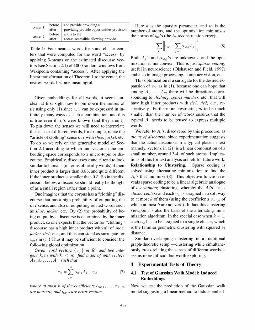
Table 1: Four nearest words for some cluster cen-ters that were computed for the word “access” byapplying 5-means on the estimated discourse vec-tors (see Section 2.1) of 1000 random windows fromWikipedia containing “access”. After applying thelinear transformation of Theorem 1 to the center, thenearest words become meaningful.

Given embeddings for all words, it seems un-clear at first sight how to pin down the senses oftie using only (1) since vtie can be expressed in in-finitely many ways as such a combination, and thisis true even if αi’s were known (and they aren’t).To pin down the senses we will need to interrelatethe senses of different words, for example, relate the“article of clothing” sense tie1 with shoe, jacket, etc.To do so we rely on the generative model of Sec-tion 2.1 according to which unit vector in the em-bedding space corresponds to a micro-topic or dis-course. Empirically, discourses c and c′ tend to looksimilar to humans (in terms of nearby words) if theirinner product is larger than 0.85, and quite differentif the inner product is smaller than 0.5. So in the dis-cussion below, a discourse should really be thoughtof as a small region rather than a point.

One imagines that the corpus has a “clothing” dis-course that has a high probability of outputting thetie1 sense, and also of outputting related words suchas shoe, jacket, etc. By (2) the probability of be-ing output by a discourse is determined by the innerproduct, so one expects that the vector for “clothing”discourse has a high inner product with all of shoe,jacket, tie1, etc., and thus can stand as surrogate forvtie1 in (1)! Thus it may be sufficient to consider thefollowing global optimization:

Given word vectors {vw} in ℜd and two inte-gers k, m with k < m, find a set of unit vectorsA1, A2, . . . , Am such that

vw =

m∑

j=1

αw,jAj + ηw (7)

where at most k of the coefficients αw,1, . . . , αw,m

are nonzero, and ηw’s are error vectors.

Here k is the sparsity parameter, and m is thenumber of atoms, and the optimization minimizesthe norms of ηw’s (the ℓ2-reconstruction error):

∑

w

∥∥∥∥vw −m∑

j=1

αw,jAj

∥∥∥∥2

2

. (8)

Both Aj’s and αw,j’s are unknowns, and the opti-mization is nonconvex. This is just sparse coding,useful in neuroscience (Olshausen and Field, 1997)and also in image processing, computer vision, etc.

This optimization is a surrogate for the desired ex-pansion of vtie as in (1), because one can hope thatamong A1, . . . , Am there will be directions corre-sponding to clothing, sports matches, etc., that willhave high inner products with tie1, tie2, etc., re-spectively. Furthermore, restricting m to be muchsmaller than the number of words ensures that thetypical Ai needs to be reused to express multiplewords.

We refer to Ai’s, discovered by this procedure, asatoms of discourse, since experimentation suggeststhat the actual discourse in a typical place in text(namely, vector c in (2)) is a linear combination of asmall number, around 3-4, of such atoms. Implica-tions of this for text analysis are left for future work.Relationship to Clustering. Sparse coding issolved using alternating minimization to find theAi’s that minimize (8). This objective function re-veals sparse coding to be a linear algebraic analogueof overlapping clustering, whereby the Ai’s act ascluster centers and each vw is assigned in a soft wayto at most k of them (using the coefficients αw,j , ofwhich at most k are nonzero). In fact this clusteringviewpoint is also the basis of the alternating mini-mization algorithm. In the special case when k = 1,each vw has to be assigned to a single cluster, whichis the familiar geometric clustering with squared ℓ2

distance.Similar overlapping clustering in a traditional

graph-theoretic setup —clustering while simultane-ously cross-relating the senses of different words—seems more difficult but worth exploring.

4 Experimental Tests of Theory

4.1 Test of Gaussian Walk Model: InducedEmbeddings

Now we test the prediction of the Gaussian walkmodel suggesting a linear method to induce embed-

487

#paragraphs 250k 500k 750k 1 millioncos similarity 0.94 0.95 0.96 0.96

Table 2: Fitting the GloVe word vectors with aver-age discourse vectors using a linear transformation.The first row is the number of paragraphs used tocompute the discourse vectors, and the second rowis the average cosine similarities between the fittedvectors and the GloVe vectors.

dings from the context of a word. Start with theGloVe embeddings; let vw denote the embeddingfor w. Randomly sample many paragraphs fromWikipedia, and for each word w′ and each occur-rence of w′ compute the SIF embedding of text inthe window of 20 words centered around w′. Aver-age the SIF embeddings for all occurrences of w′ toobtain vector uw′ . The Gaussian walk model saysthat there is a linear transformation that maps uw′ tovw′ , so solve the regression:

argminA

∑

w

∥Auw − vw∥22. (9)

We call the vectors Auw the induced embeddings.We can test this method of inducing embeddings byholding out 1/3 words randomly, doing the regres-sion (9) on the rest, and computing the cosine sim-ilarities between Auw and vw on the heldout set ofwords.

Table 2 shows that the average cosine similar-ity between the induced embeddings and the GloVevectors is large. By contrast the average similar-ity between the average discourse vectors and theGloVe vectors is much smaller (about 0.58), illus-trating the need for the linear transformation. Sim-ilar results are observed for the word2vec and SNvectors (Arora et al., 2016).

4.2 Test of Linearity Assertion

We do two empirical tests of the Linearity Assertion(Theorem 2).Test 1. The first test involves the classic artificialpolysemous words (also called pseudowords). First,pre-train a set W1 of word vectors on Wikipedia withexisting embedding methods. Then, randomly pickm pairs of non-repeated words, and for each pair,replace each occurrence of either of the two words

m pairs 10 103 3 · 104

relative errorSN 0.32 0.63 0.67

GloVe 0.29 0.32 0.51

cos similaritySN 0.90 0.72 0.75

GloVe 0.91 0.91 0.77

Table 3: The average relative errors and cosine sim-ilarities between the vectors of pseudowords andthose predicted by Theorem 2. m pairs of words arerandomly selected and for each pair, all occurrencesof the two words in the corpus is replaced by a pseu-doword. Then train the vectors for the pseudowordson the new corpus.

with a pseudoword. Third, train a set W2 of vectorson the new corpus, while holding fixed the vectorsof words that were not involved in the pseudowords.Construction has ensured that each pseudoword hastwo distinct “senses”, and we also have in W1 the“ground truth” vectors for those senses.2 Theorem 2implies that the embedding of a pseudoword is a lin-ear combination of the sense vectors, so we can com-pare this predicted embedding to the one learned inW2.3

Suppose the trained vector for a pseudoword wis uw and the predicted vector is vw, then thecomparison criterion is the average relative error1

|S|∑

w∈S∥uw−vw∥2

2

∥vw∥22

where S is the set of all thepseudowords. We also report the average cosinesimilarity between vw’s and uw’s.

Table 3 shows the results for the GloVe andSN (Arora et al., 2016) vectors, averaged over 5runs. When m is small, the error is small and the co-sine similarity is as large as 0.9. Even if m = 3 ·104

2Note that this discussion assumes that the set of pseu-dowords is small, so that a typical neighborhood of a pseu-doword does not consist of other pseudowords. Otherwise theground truth vectors in W1 become a bad approximation to thesense vectors.

3Here W2 is trained while fixing the vectors of words notinvolved in pseudowords to be their pre-trained vectors in W1.We can also train all the vectors in W2 from random initializa-tion. Such W2 will not be aligned with W1. Then we can learna linear transformation from W2 to W1 using the vectors for thewords not involved in pseudowords, apply it on the vectors forthe pseudowords, and compare the transformed vectors to thepredicted ones. This is tested on word2vec, resulting in relativeerrors between 20% and 32%, and cosine similarities between0.86 and 0.92. These results again support our analysis.

488

vector type GloVe skip-gram SNcosine 0.72 0.73 0.76

Table 4: The average cosine of the angles betweenthe vectors of words and the span of vector represen-tations of its senses. The words tested are those inthe WSI task of SemEval 2010.

(i.e., about 90% of the words in the vocabulary arereplaced by pseudowords), the cosine similarity re-mains above 0.7, which is significant in the 300 di-mensional space. This provides positive support forour analysis.Test 2. The second test is a proxy for what wouldbe a complete (but laborious) test of the LinearityAssertion: replicating the thought experiment whilehand-labeling sense usage for many words in a cor-pus. The simpler proxy is as follows. For eachword w, WordNet (Fellbaum, 1998) lists its vari-ous senses by providing definition and example sen-tences for each sense. This is enough text (roughlya paragraph’s worth) for our theory to allow us torepresent it by a vector —specifically, apply the SIFsentence embedding followed by the linear transfor-mation learned as in Section 4.1. The text embed-ding for sense s should approximate the ground truthvector vs for it. Then the Linearity Assertion pre-dicts that embedding vw lies close to the subspacespanned by the sense vectors. (Note that this is anontrivial event: in 300 dimensions a random vectorwill be quite far from the subspace spanned by some3 other random vectors.) Table 4 checks this predic-tion using the polysemous words appearing in theWSI task of SemEval 2010. We tested three stan-dard word embedding methods: GloVe, the skip-gram variant of word2vec, and SN (Arora et al.,2016). The results show that the word vectors arequite close to the subspace spanned by the senses.

5 Experiments with Atoms of Discourse

The experiments use 300-dimensional embeddingscreated using the SN objective in (Arora et al., 2016)and a Wikipedia corpus of 3 billion tokens (Wikime-dia, 2012), and the sparse coding is solved by stan-dard k-SVD algorithm (Damnjanovic et al., 2010).Experimentation showed that the best sparsity pa-rameter k (i.e., the maximum number of allowed

senses per word) is 5, and the number of atoms mis about 2000. For the number of senses k, wetried plausible alternatives (based upon suggestionsof many colleagues) that allow k to vary for differ-ent words, for example to let k be correlated with theword frequency. But a fixed choice of k = 5 seemsto produce just as good results. To understand why,realize that this method retains no information aboutthe corpus except for the low dimensional word em-beddings. Since the sparse coding tends to expressa word using fairly different atoms, examining (7)shows that

∑j α2

w,j is bounded by approximately∥vw∥22. So if too many αw,j’s are allowed to benonzero, then some must necessarily have small co-efficients, which makes the corresponding compo-nents indistinguishable from noise. In other words,raising k often picks not only atoms correspondingto additional senses, but also many that don’t.

The best number of atoms m was found to bearound 2000. This was estimated by re-runningthe sparse coding algorithm multiple times with dif-ferent random initializations, whereupon substantialoverlap was found between the two bases: a largefraction of vectors in one basis were found to havea very close vector in the other. Thus combiningthe bases while merging duplicates yielded a basis ofabout the same size. Around 100 atoms are used bya large number of words or have no close-by words.They appear semantically meaningless and are ex-cluded by checking for this condition.4

The content of each atom can be discerned bylooking at the nearby words in cosine similarity.Some examples are shown in Table 5. Each word isrepresented using at most five atoms, which usuallycapture distinct senses (with some noise/mistakes).The senses recovered for tie and spring are shownin Table 6. Similar results can be obtained by usingother word embeddings like word2vec and GloVe.

We also observe sparse coding procedures assignnonnegative values to most coefficients αw,j’s evenif they are left unrestricted. Probably this is becausethe appearances of a word are best explained by whatdiscourse is being used to generate it, rather thanwhat discourses are not being used.

4We think semantically meaningless atoms —i.e., unex-plained inner products—exist because a simple language modelsuch as ours cannot explain all observed co-occurrences due togrammar, stopwords, etc. It ends up needing smoothing terms.

489

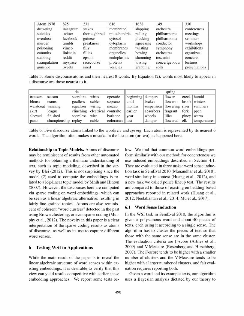
Atom 1978 825 231 616 1638 149 330drowning instagram stakes membrane slapping orchestra conferencessuicides twitter thoroughbred mitochondria pulling philharmonic meetingsoverdose facebook guineas cytosol plucking philharmonia seminarsmurder tumblr preakness cytoplasm squeezing conductor workshopspoisoning vimeo filly membranes twisting symphony exhibitionscommits linkedin fillies organelles bowing orchestras organizesstabbing reddit epsom endoplasmic slamming toscanini concertsstrangulation myspace racecourse proteins tossing concertgebouw lecturesgunshot tweets sired vesicles grabbing solti presentations

Table 5: Some discourse atoms and their nearest 9 words. By Equation (2), words most likely to appear ina discourse are those nearest to it.

tie springtrousers season scoreline wires operatic beginning dampers flower creek humidblouse teams goalless cables soprano until brakes flowers brook winterswaistcoat winning equaliser wiring mezzo months suspension flowering river summersskirt league clinching electrical contralto earlier absorbers fragrant fork ppensleeved finished scoreless wire baritone year wheels lilies piney warmpants championship replay cable coloratura last damper flowered elk temperatures

Table 6: Five discourse atoms linked to the words tie and spring. Each atom is represented by its nearest 6words. The algorithm often makes a mistake in the last atom (or two), as happened here.

Relationship to Topic Models. Atoms of discoursemay be reminiscent of results from other automatedmethods for obtaining a thematic understanding oftext, such as topic modeling, described in the sur-vey by Blei (2012). This is not surprising since themodel (2) used to compute the embeddings is re-lated to a log-linear topic model by Mnih and Hinton(2007). However, the discourses here are computedvia sparse coding on word embeddings, which canbe seen as a linear algebraic alternative, resulting infairly fine-grained topics. Atoms are also reminis-cent of coherent “word clusters” detected in the pastusing Brown clustering, or even sparse coding (Mur-phy et al., 2012). The novelty in this paper is a clearinterpretation of the sparse coding results as atomsof discourse, as well as its use to capture differentword senses.

6 Testing WSI in Applications

While the main result of the paper is to reveal thelinear algebraic structure of word senses within ex-isting embeddings, it is desirable to verify that thisview can yield results competitive with earlier senseembedding approaches. We report some tests be-

low. We find that common word embeddings per-form similarly with our method; for concreteness weuse induced embeddings described in Section 4.1.They are evaluated in three tasks: word sense induc-tion task in SemEval 2010 (Manandhar et al., 2010),word similarity in context (Huang et al., 2012), anda new task we called police lineup test. The resultsare compared to those of existing embedding basedapproaches reported in related work (Huang et al.,2012; Neelakantan et al., 2014; Mu et al., 2017).

6.1 Word Sense InductionIn the WSI task in SemEval 2010, the algorithm isgiven a polysemous word and about 40 pieces oftexts, each using it according to a single sense. Thealgorithm has to cluster the pieces of text so thatthose with the same sense are in the same cluster.The evaluation criteria are F-score (Artiles et al.,2009) and V-Measure (Rosenberg and Hirschberg,2007). The F-score tends to be higher with a smallernumber of clusters and the V-Measure tends to behigher with a larger number of clusters, and fair eval-uation requires reporting both.

Given a word and its example texts, our algorithmuses a Bayesian analysis dictated by our theory to

490

compute a vector uc for each piece of text c andand then applies k-means on these vectors, with thesmall twist that sense vectors are assigned to near-est centers based on inner products rather than Eu-clidean distances. Table 7 shows the results.Computing vector uc. For word w we start by com-puting its expansion in terms of atoms of discourse(see (8) in Section 3). In an ideal world the nonzerocoefficients would exactly capture its senses, andeach text containing w would match to one of thesenonzero coefficients. In the real world such deter-ministic success is elusive and one must reason us-ing Bayes’ rule.

For each atom a, word w and text c there is a jointdistribution p(w, a, c) describing the event that atoma is the sense being used when word w was used intext c. We are interested in the posterior distribution:

p(a|c, w) ∝ p(a|w)p(a|c)/p(a). (10)

We approximate p(a|w) using Theorem 2, whichsuggests that the coefficients in the expansion of vw

with respect to atoms of discourse scale according toprobabilities of usage. (This assertion involves ig-noring the low-order terms involving the logarithmin the theorem statement.) Also, by the random walkmodel, p(a|c) can be approximated by exp(⟨va, vc⟩)where vc is the SIF embedding of the context. Fi-nally, since p(a) = Ec[p(a|c)], it can be empiricallyestimated by randomly sampling c.

The posterior p(a|c, w) can be seen as a soft de-coding of text c to atom a. If texts c1, c2 both containw, and they were hard decoded to atoms a1, a2 re-spectively then their similarity would be ⟨va1 , va2⟩.With our soft decoding, the similarity can be definedby taking the expectation over the full posterior:

similarity(c1, c2)

= Eai∼p(a|ci,w),i∈{1,2}⟨va1 , va2⟩, (11)

=

⟨∑

a1

p(a1|c1, w)va1 ,∑

a2

p(a2|c2, w)va2

⟩.

At a high level this is analogous to the Bayesianpolysemy model of Reisinger and Mooney (2010)and Brody and Lapata (2009), except that they in-troduced separate embeddings for each sense clus-ter, while here we are working with structure alreadyexisting inside word embeddings.

Method V-Measure F-Score(Huang et al., 2012) 10.60 38.05

(Neelakantan et al., 2014) 9.00 47.26(Mu et al., 2017), k = 2 7.30 57.14(Mu et al., 2017), k = 5 14.50 44.07

ours, k = 2 6.1 58.55ours, k = 3 7.4 55.75ours, k = 4 9.9 51.85ours, k = 5 11.5 46.38

Table 7: Performance of different vectors in the WSItask of SemEval 2010. The parameter k is the num-ber of clusters used in the methods. Rows are di-vided into two blocks, the first of which shows theresults of the competitors, and the second showsthose of our algorithm. Best results in each blockare in boldface.

The last equation suggests defining the vector uc

for the text c as

uc =∑

a

p(a|c, w)va, (12)

which allows the similarity between two text piecesto be expressed via the inner product of their vectors.Results. The results are reported in Table 7. Ourapproach outperforms the results by Huang et al.(2012) and Neelakantan et al. (2014). When com-pared to Mu et al. (2017), for the case with 2 centers,we achieved better V-measure but lower F-score,while for 5 centers, we achieved lower V-measurebut better F-score.

6.2 Word Similarity in Context

The dataset consists of around 2000 pairs of words,along with the contexts the words occur in and theground-truth similarity scores. The evaluation cri-terion is the correlation between the ground-truthscores and the predicted ones. Our method computesthe estimated sense vectors and then the similarity asin Section 6.1. We compare to the baselines that sim-ply use the cosine similarity of the GloVe/skip-gramvectors, and also to the results of several existingsense embedding methods.Results. Table 8 shows that our result is betterthan those of the baselines and Mu et al. (2017),but slightly worse than that of Huang et al. (2012).

491

Method Spearman coefficientGloVe 0.573

skip-gram 0.622(Huang et al., 2012) 0.657

(Neelakantan et al., 2014) 0.567(Mu et al., 2017) 0.637

ours 0.652

Table 8: The results for different methods in the taskof word similarity in context. The best result is inboldface. Our result is close to the best.

Note that Huang et al. (2012) retrained the vectorsfor the senses on the corpus, while our method de-pends only on senses extracted from the off-the-shelfvectors. After all, our goal is to show word sensesalready reside within off-the-shelf word vectors.

6.3 Police Lineup

Evaluating WSI systems can run into well-knowndifficulties, as reflected in the changing metrics overthe years (Navigli and Vannella, 2013). Inspired byword-intrusion tests for topic coherence (Chang etal., 2009), we proposed a new simple test, which hasthe advantages of being easy to understand, and ca-pable of being administered to humans.

The testbed uses 200 polysemous words and their704 senses according to WordNet. Each sense isrepresented by 8 related words, which were col-lected from WordNet and online dictionaries by col-lege students, who were told to identify most rele-vant other words occurring in the online definitionsof this word sense as well as in the accompany-ing illustrative sentences. These are considered asground truth representation of the word sense. These8 words are typically not synonyms. For example,for the tool/weapon sense of axe they were “handle,harvest, cutting, split, tool, wood, battle, chop.”

The quantitative test is called police lineup. First,randomly pick one of these 200 polysemous words.Second, pick the true senses for the word and thenadd randomly picked senses from other words sothat there are n senses in total, where each sense isrepresented by 8 related words as mentioned. Fi-nally, the algorithm (or human) is given the polyse-mous word and a set of n senses, and has to identifythe true senses in this set. Table 9 gives an example.

word senses

bat

1 navigate nocturnal mouse wing cave sonic fly dark2 used hitting ball game match cricket play baseball3 wink briefly shut eyes wink bate quickly action4 whereby legal court law lawyer suit bill judge5 loose ends two loops shoelaces tie rope string6 horny projecting bird oral nest horn hard food

Table 9: An example of the police lineup test withn = 6. The algorithm (or human subject) is giventhe polysemous word “bat” and n = 6 senses each ofwhich is represented as a list of words, and is askedto identify the true senses belonging to “bat” (high-lighted in boldface for demonstration).

Algorithm 1 Our method for the police lineup testInput: Word w, list S of senses (each has 8 words)Output: t senses out of S

1: Heuristically find inflectional forms of w.2: Find 5 atoms for w and each inflectional form. Let

U denote the union of all these atoms.3: Initialize the set of candidate senses Cw ← ∅, and

the score for each sense L to score(L)← −∞4: for each atom a ∈ U do5: Rank senses L ∈ S by

score(a, L)=s(a, L)−sLA + s(w, L)− sL

V

6: Add the two senses L with highest score(a, L) toCw, and update their scores

score(L)← max{score(L), score(a, L)}7: Return the t senses L ∈ Cs with highest score(L)

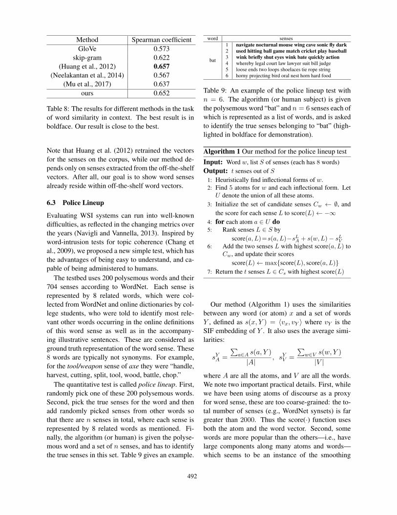
Our method (Algorithm 1) uses the similaritiesbetween any word (or atom) x and a set of wordsY , defined as s(x, Y ) = ⟨vx, vY ⟩ where vY is theSIF embedding of Y . It also uses the average simi-larities:

sYA =

∑a∈A s(a, Y )

|A| , sYV =

∑w∈V s(w, Y )

|V |where A are all the atoms, and V are all the words.We note two important practical details. First, whilewe have been using atoms of discourse as a proxyfor word sense, these are too coarse-grained: the to-tal number of senses (e.g., WordNet synsets) is fargreater than 2000. Thus the score(·) function usesboth the atom and the word vector. Second, somewords are more popular than the others—i.e., havelarge components along many atoms and words—which seems to be an instance of the smoothing

492

0 0.2 0.4 0.6 0.8 1Recall

0

0.2

0.4

0.6

0.8

1

Pre

cisi

on

Our methodMu et al, 2017word2vecNative speakerNon-native speaker

10 20 30 40 50 60 70 80Number of meanings m

0

0.2

0.4

0.6

0.8

1

RecallPrecision

A BFigure 1: Precision and recall in the police lineup test. (A) For each polysemous word, a set of n = 20 sensescontaining the ground truth senses of the word are presented. Human subjects are told that on average eachword has 3.5 senses and were asked to choose the senses they thought were true. The algorithms select tsenses for t = 1, 2, . . . , 6. For each t, each algorithm was run 5 times (standard deviations over the runs aretoo small to plot). (B) The performance of our method for t = 4 and n = 20, 30, . . . , 70.

phenomenon alluded to in Footnote 4. The penaltyterms sL

A and sLV lower the scores of senses L con-

taining such words. Finally, our algorithm returns tsenses where t can be varied.Results. The precision and recall for different n andt (number of senses the algorithm returns) are pre-sented in Figure 1. Our algorithm outperforms thetwo selected competitors. For n = 20 and t = 4,our algorithm succeeds with precision 65% and re-call 75%, and performance remains reasonable forn = 50. Giving the same test to humans5 for n = 20(see the left figure) suggests that our method per-forms similarly to non-native speakers.

Other word embeddings can also be used in thetest and achieved slightly lower performance. Forn = 20 and t = 4, the precision/recall are lower bythe following amounts: GloVe 2.3%/5.76%, NNSE(matrix factorization on PMI to rank 300 by Murphyet al. (2012)) 25%/28%.

7 Conclusions

Different senses of polysemous words have beenshown to lie in linear superposition inside standardword embeddings like word2vec and GloVe. Thishas also been shown theoretically building upon

5Human subjects are graduate students from science or engi-neering majors at major U.S. universities. Non-native speakershave 7 to 10 years of English language use/learning.

previous generative models, and empirical tests ofthis theory were presented. A priori, one imaginesthat showing such theoretical results about the in-ner structure of modern word embeddings wouldbe hopeless since they are solutions to complicatednonconvex optimization.

A new WSI method is also proposed based uponthese insights that uses only the word embeddingsand sparse coding, and shown to provide very com-petitive performance on some WSI benchmarks.One novel aspect of our approach is that the wordsenses are interrelated using one of about 2000 dis-course vectors that give a succinct description ofwhich other words appear in the neighborhood withthat sense. Our method based on sparse coding canbe seen as a linear algebraic analog of the cluster-ing approaches, and also gives fine-grained thematicstructure reminiscent of topic models.

A novel police lineup test was also proposed fortesting such WSI methods, where the algorithm isgiven a word w and word clusters, some of whichbelong to senses of w and the others are distractorsbelonging to senses of other words. The algorithmhas to identify the ones belonging to w. We con-jecture this police lineup test with distractors willchallenge some existing WSI methods, whereas ourmethod was found to achieve performance similar tonon-native speakers.

493

Acknowledgements

We thank the reviewers and the action editor of TACL for helpful feedback and thank the editors for granting special relaxation of the page limit for our paper. This work was supported in part by NSF grants CCF-1527371, DMS-1317308, Simons In-vestigator Award, Simons Collaboration Grant, and ONR-N00014-16-1-2329. Tengyu Ma was addition-ally supported by the Simons Award in Theoretical Computer Science and by the IBM Ph.D. Fellow-ship.

ReferencesSanjeev Arora, Yuanzhi Li, Yingyu Liang, Tengyu Ma,

and Andrej Risteski. 2016. A latent variable modelapproach to PMI-based word embeddings. Trans-action of Association for Computational Linguistics,pages 385–399.

Sanjeev Arora, Yingyu Liang, and Tengyu Ma. 2017. Asimple but tough-to-beat baseline for sentence embed-dings. In In Proceedings of International Conferenceon Learning Representations.

Javier Artiles, Enrique Amigo, and Julio Gonzalo. 2009.The role of named entities in web people search. InProceedings of the 2009 Conference on EmpiricalMethods in Natural Language Processing, pages 534–542.

Yoshua Bengio, Rejean Ducharme, Pascal Vincent, andChristian Jauvin. 2003. A neural probabilistic lan-guage model. Journal of Machine Learning Research,pages 1137–1155.

David M. Blei. 2012. Probabilistic topic models. Com-munication of the Association for Computing Machin-ery, pages 77–84.

Samuel Brody and Mirella Lapata. 2009. Bayesian wordsense induction. In Proceedings of the 12th Confer-ence of the European Chapter of the Association forComputational Linguistics, pages 103–111.

Jonathan Chang, Sean Gerrish, Chong Wang, Jordan L.Boyd-Graber, and David M. Blei. 2009. Readingtea leaves: How humans interpret topic models. InAdvances in Neural Information Processing Systems,pages 288–296.

Kenneth Ward Church and Patrick Hanks. 1990. Wordassociation norms, mutual information, and lexicogra-phy. Computational linguistics, pages 22–29.

Ivan Damnjanovic, Matthew Davies, and Mark Plumb-ley. 2010. SMALLbox – an evaluation frameworkfor sparse representations and dictionary learning al-gorithms. In International Conference on Latent Vari-able Analysis and Signal Separation, pages 418–425.

Antonio Di Marco and Roberto Navigli. 2013. Clus-tering and diversifying web search results with graph-based word sense induction. Computational Linguis-tics, pages 709–754.

Manaal Faruqui, Yulia Tsvetkov, Dani Yogatama, ChrisDyer, and Noah A. Smith. 2015. Sparse overcompleteword vector representations. In Proceedings of As-sociation for Computational Linguistics, pages 1491–1500.

Christiane Fellbaum. 1998. WordNet: An ElectronicLexical Database. MIT Press.

John Rupert Firth. 1957. A synopsis of linguistic theory,1930-1955. Studies in Linguistic Analysis.

Alex Gittens, Dimitris Achlioptas, and Michael W Ma-honey. 2017. Skip-gram – Zipf + Uniform = VectorAdditivity. In Proceedings of the 55th Annual Meet-ing of the Association for Computational Linguistics(Volume 1: Long Papers), volume 1, pages 69–76.

Thomas L. Griffiths, Mark Steyvers, and Joshua B.Tenenbaum. 2007. Topics in semantic representation.Psychological review, pages 211–244.

Eric H. Huang, Richard Socher, Christopher D. Manning,and Andrew Y. Ng. 2012. Improving word representa-tions via global context and multiple word prototypes.In Proceedings of the 50th Annual Meeting of the Asso-ciation for Computational Linguistics, pages 873–882.

Ignacio Iacobacci, Mohammad Taher Pilehvar, andRoberto Navigli. 2015. SensEmbed: Learning senseembeddings for word and relational similarity. In Pro-ceedings of Association for Computational Linguis-tics, pages 95–105.

Omer Levy and Yoav Goldberg. 2014. Neural wordembedding as implicit matrix factorization. In Ad-vances in Neural Information Processing Systems,pages 2177–2185.

Suresh Manandhar, Ioannis P Klapaftis, Dmitriy Dligach,and Sameer S Pradhan. 2010. SemEval 2010: Task14: Word sense induction & disambiguation. In Pro-ceedings of the 5th International Workshop on Seman-tic Evaluation, pages 63–68.

Tomas Mikolov, Ilya Sutskever, Kai Chen, Greg S. Cor-rado, and Jeff Dean. 2013a. Distributed represen-tations of words and phrases and their composition-ality. In Advances in Neural Information ProcessingSystems, pages 3111–3119.

Tomas Mikolov, Wen-tau Yih, and Geoffrey Zweig.2013b. Linguistic regularities in continuous spaceword representations. In Proceedings of the Confer-ence of the North American Chapter of the Associa-tion for Computational Linguistics: Human LanguageTechnologies, pages 746–751.

Andriy Mnih and Geoffrey Hinton. 2007. Three newgraphical models for statistical language modelling. In

494

Proceedings of the 24th International Conference onMachine Learning, pages 641–648.

Jiaqi Mu, Suma Bhat, and Pramod Viswanath. 2017. Ge-ometry of polysemy. In Proceedings of InternationalConference on Learning Representations.

Brian Murphy, Partha Pratim Talukdar, and Tom M.Mitchell. 2012. Learning effective and interpretablesemantic models using non-negative sparse embed-ding. In Proceedings of the 24th International Confer-ence on Computational Linguistics, pages 1933–1950.

Roberto Navigli and Daniele Vannella. 2013. SemEval2013: Task 11: Word sense induction and disambigua-tion within an end-user application. In Second JointConference on Lexical and Computational Semantics,pages 193–201.

Arvind Neelakantan, Jeevan Shankar, Re Passos, andAndrew Mccallum. 2014. Efficient nonparametricestimation of multiple embeddings per word in vec-tor space. In Proceedings of Conference on Empiri-cal Methods in Natural Language Processing, pages1059–1069.

Bruno Olshausen and David Field. 1997. Sparse codingwith an overcomplete basis set: A strategy employedby V1? Vision Research, pages 3311–3325.

Jeffrey Pennington, Richard Socher, and Christopher D.Manning. 2014. GloVe: Global Vectors for word rep-resentation. In Proceedings of the Empiricial Methodsin Natural Language Processing, pages 1532–1543.

Joseph Reisinger and Raymond Mooney. 2010. Multi-prototype vector-space models of word meaning. InProceedings of the Conference of the North AmericanChapter of the Association for Computational Linguis-tics: Human Language Technologies, pages 107–117.

Andrew Rosenberg and Julia Hirschberg. 2007. V-measure: A conditional entropy-based external clus-ter evaluation measure. In Conference on EmpiricalMethods in Natural Language Processing and Confer-ence on Computational Natural Language Learning,pages 410–420.

Hinrich Schutze. 1998. Automatic word sense discrimi-nation. Computational Linguistics, pages 97–123.

Ran Tian, Naoaki Okazaki, and Kentaro Inui. 2017. Themechanism of additive composition. Machine Learn-ing, 106(7):1083–1130.

Peter D. Turney and Patrick Pantel. 2010. From fre-quency to meaning: Vector space models of seman-tics. Journal of Artificial Intelligence Research, pages141–188.

Wikimedia. 2012. English Wikipedia dump. AccessedMarch 2015.

David Yarowsky. 1995. Unsupervised word sense dis-ambiguation rivaling supervised methods. In Proceed-ings of the 33rd Annual Meeting on Association forComputational Linguistics, pages 189–196.

495

496