chapter 1 wave{particle duality -...

$: Chapter 1 Wave{Particle Duality - univie.ac.athomepage.univie.ac.at/Reinhold.Bertlmann/pdfs/T2_Skript...Chapter 1 Wave{Particle Duality 1.1 Planck’s Law of Black Body Radiation 1.1.1$
Chapter 1

Wave–Particle Duality

1.1 Planck’s Law of Black Body Radiation

1.1.1 Quantization of Energy

The foundation of quantum mechanics was laid in 1900 with Max Planck’s discovery of thequantized nature of energy. When Planck developed his formula for black body radiationhe was forced to assume that the energy exchanged between a black body and its thermal(electromagnetic) radiation is not a continuous quantity but needs to be restricted todiscrete values depending on the (angular-) frequency of the radiation. Planck’s formulacan explain – as we shall see – all features of the black body radiation and his finding isphrased in the following way:

Proposition 1.1.1 Energy is quantized and given in units of ~ω. E = ~ω

Here ω denotes the angular frequency ω = 2πν. We will drop the prefix ”angular”in the following and only refer to it as the frequency. We will also bear in mind theconnection to the wavelength λ given by c = λν, where c is the speed of light, and to theperiod T given by ν = 1

T.

The fact that the energy is proportional to the frequency, rather than to the intensityof the wave – what we would expect from classical physics – is quite counterintuitive. Theproportionality constant ~ is called Planck’s constant :

~ =h

2π= 1, 054× 10−34 Js = 6, 582× 10−16 eVs (1.1)

h = 6, 626× 10−34 Js = 4, 136× 10−15 eVs . (1.2)

1

2 CHAPTER 1. WAVE–PARTICLE DUALITY

1.1.2 Black Body Radiation

A black body is by definition an object that completely absorbs all light (radiation) thatfalls on it. This property makes a black body a perfect source of thermal radiation. A verygood realization of a black body is an oven with a small hole, see Fig. 1.1. All radiationthat enters through the opening has a very small probability of leaving through it again.

Figure 1.1: Scheme for realization of a black body as a cavity

Thus the radiation coming from the opening is just the thermal radiation, which willbe measured in dependence of its frequency and the oven temperature as shown in Fig. 1.2.Such radiation sources are also referred to as (thermal) cavities.

The classical law that describes such thermal radiation is the Rayleigh-Jeans law whichexpresses the energy density u(ω) in terms of frequency ω and temperature T .

Theorem 1.1 (Rayleigh-Jeans law) u(ω) = kTπ2c3 ω

2

where k denotes Boltzmann’s constant, k = 1, 38× 10−23 J K−1.

Boltzmann’s constant plays a role in classical thermo-statistics where (ideal) gases areanalyzed whereas here we describe radiation. The quantity kT has the dimension of en-ergy, e.g., in a classical system in thermal equilibrium, each degree of freedom (of motion)has a mean energy of E = 1

2kT – Equipartition Theorem.

From the expression of Theorem 1.1 we immediately see that the integral of the energydensity over all possible frequencies is divergent,∫ ∞

0

dω u(ω)→∞ , (1.3)

1.1. PLANCK’S LAW OF BLACK BODY RADIATION 3

Figure 1.2: Spectrum of a black body for different temperatures, picture from:http://commons.wikimedia .org/wiki/Image:BlackbodySpectrum lin 150dpi en.png

which would imply an infinite amount of energy in the black body radiation. This isknown as the ultraviolet catastrophe and the law is therefore only valid for small frequen-cies.

For high frequencies a law was found empirically by Wilhelm Wien in 1896.

Theorem 1.2 (Wien’s law) u(ω)→ Aω3e−BωT for ω →∞

where A and B are constants which we will specify later on.

As already mentioned Max Planck derived an impressive formula which interpolates1

between the Rayleigh-Jeans law and Wien’s law. For the derivation the correctness ofProposition 1.1.1 was necessary, i.e., the energy can only occur in quanta of ~ω. For thisachievement he was awarded the 1919 nobel prize in physics.

1See Fig. 1.3


Theorem 1.3 (Planck’s law) u(ω) = ~π2c3

ω3

exp (~ωkT )− 1

From Planck’s law we arrive at the already well-known laws of Rayleigh-Jeans andWien by taking the limits for ω → 0 or ω →∞ respectively:

for ω → 0 → Rayleigh-Jeans

u(ω) = ~π2c3

ω3

exp ( ~ωkT

)− 1

for ω →∞ → Wien

Figure 1.3: Comparison of the radiation laws of Planck, Wien and Rayleigh-Jeans, picturefrom: http://en.wikipedia.org/wiki/Image:RWP-comparison.svg

We also want to point out some of the consequences of Theorem 1.3.

• Wien’s displacement law: λmaxT = const. = 0, 29 cm K

• Stefan-Boltzmann law: for the radiative power we have∫ ∞0

dω u(ω) ∝ T 4

∫ ∞0

d(~ωkT

)( ~ωkT

)3

exp ( ~ωkT

) − 1(1.4)

1.1. PLANCK’S LAW OF BLACK BODY RADIATION 5

substituting ~ωkT

= x and using formula∫ ∞0

dxx3

ex − 1=

π4

15(1.4)

we find the proportionality ∝ T 4

1.1.3 Derivation of Planck’s Law

Now we want to derive Planck’s law by considering a black body realized by a hollowmetal ball. We assume the metal to be composed of two energy-level atoms such thatthey can emit or absorb photons with energy E = ~ω as sketched in Fig. 1.4.

Figure 1.4: Energy states in a two level atom, e... excited state, g... ground state. Thereare three processes: absorption, stimulated emission and spontaneous emission of photons.

Further assuming thermal equilibrium, the number of atoms in ground and excitedstates is determined by the (classical) Boltzmann distribution of statistical mechanics

Ne

Ng

= exp

(− E

kT

), (1.5)

where Ne/g is the number of excited/non-excited atoms and T is the thermodynamicaltemperature of the system.

As Einstein first pointed out there are three processes: the absorption of photons,the stimulated emission and the spontaneous emission of photons from the excited stateof the atom, see Fig. 1.4. The stimulated processes are proportional to the number ofphotons whereas the spontaneous process is not, it is just proportional to the transitionrate. Furthermore, the coefficients of absorption and stimulated emission are assumed toequal and proportional to the probability of spontaneous emission.

Now, in the thermal equilibrium the rates for emission and absorption of a photonmust be equal and thus we can conclude that:


Absorption rate: Ng nP P ... probability for transition

Emission rate: Ne (n+ 1)P n ... average number of photons

⇒

Ng nP = Ne (n+ 1)P ⇒ n

n+ 1=

Ne

Ng

= exp

(− E

kT

)= exp

(−~ωkT

)

providing the average number of photons in the cavern2

n =1

e~ωkT − 1

, (1.6)

and the average photon energy

n ~ω =~ω

e~ωkT − 1

. (1.7)

Turning next to the energy density we need to consider the photons as standing wavesinside the hollow ball due to the periodic boundary conditions imposed on the system bythe cavern walls. We are interested in the number of possible modes of the electromagneticfield inside an infinitesimal element dk, where k = 2π

λ= ω

cis the wave number.

Figure 1.5: Photon described as standing wave in a cavern of length L.

The number of knots N (wavelengths) of this standing wave is then given by

N =L

λ=

L

2π

2π

λ=

L

2πk , (1.8)

which gives within an infinitesimal element

1-dim: dN =L

2πdk 3-dim: dN = 2

V

(2π)3d3k , (1.9)

where we inserted in 3 dimensions a factor 2 for the two (polarization) degrees of freedom ofthe photon and wrote L3 as V, the volume of the cell. Furthermore, inserting d3k = 4πk2dkand using the relation k = ω

cfor the wave number we get

dN = 2V

(2π)3

4πω2dω

c3. (1.10)

We will now calculate the energy density of the photons.

2Note that in our derivation P corresponds to the Einstein coefficient A and nP to the Einsteincoefficient B in Quantum Optics.

1.2. THE PHOTOELECTRIC EFFECT 7

1. Classically: In the classical case we follow the equipartition theorem, telling usthat in thermal equilibrium each degree of freedom contributes E = 1

2kT to the

total energy of the system, though, as we shall encounter, it does not hold true forquantum mechanical systems, especially for low temperatures.

Considering the standing wave as harmonic oscillator has the following mean energy:

E = 〈Ekin〉+ 〈V 〉 =⟨m

2v2⟩

+⟨mω

2x2⟩

=1

2kT +

1

2kT = kT . (1.11)

For the oscillator the mean kinetic and potential energy are equal3, 〈Ekin〉 = 〈V 〉,and both are proportional to quadratic variables which is the equipartition theorem’scriterion for a degree of freedom to contribute 1

2kT . We thus can write dE = kT dN

and by taking equation (1.10) we calculate the (spectral) energy density

u(ω) =1

V

dE

dω=

kT

π2c3ω2 , (1.12)

which we recognize as Theorem 1.1, the Rayleigh-Jeans Law.

2. Quantum-mechanically: In the quantum case we use the average photon energy,equation (1.7), we calculated above by using the quantization hypothesis, Proposi-tion 1.1.1, to write dE = n ~ω dN and again inserting equation (1.10) we calculate

u(ω) =1

V

dE

dω=

~π2c3

ω3

e~ωkT − 1

, (1.13)

and we recover Theorem 1.3, Planck’s Law for black body radiation.

1.2 The Photoelectric Effect

1.2.1 Facts about the Photoelectric Effect

In 1887 Heinrich Hertz discovered a phenomenon, the photoelectric effect, that touchesthe foundation of quantum mechanics. A metal surface emits electrons when illuminatedby ultraviolet light. The importance of this discovery lies within the inability of classicalphysics to describe the effect in its full extent based on three observations.

1. ) The kinetic energy of the emitted electrons is independent of the intensity of theilluminating source of light and

2. ) increases with increasing frequency of the light.

3. ) There exists a threshold frequency below which no electrons are emitted.

3This statement results from the so-called Virial theorem, stating that 〈2Ekin〉 =⟨xdV

dx

⟩, which we

will encounter later on in Section 2.7.


More accurate measurements were made by Philipp Lenard between 1900 and 1902for which he received the nobel prize in 1905.

In terms of classical physics this effect was not understood as from classical electro-dynamics was known that the

energy density: u =1

8π

(~E2 + ~B2

)(1.14)

and the energy flux: S =c

8π~E × ~B (1.15)

are both proportional to the intensity. Thus “knocking” electrons out of the metal is pos-sible, but there is no threshold that limits this process to certain frequencies. As long asthe surface is exposed to the radiation the electrons absorb energy until they get detachedfrom the metal.

1.2.2 Einstein’s Explanation for the Photoelectric Effect

The phenomenon of the photoelectric effect could then be explained by Albert Einsteinin 1905 with his photon hypothesis which he was also awarded the nobel prize for in 1921.

Proposition 1.2.1 (Photon hypothesis)Light consists of quanta (photons) with respective energy of E = ~ω each.

Einstein explained the effect in the following way. The incident photons transfertheir energy to the electrons of the metal. Since the electrons are bound to the metalthe energy need to be sufficient to overcome the electrostatic barrier of the metal. Therespective energy, which is dependent on the material used is termed the work functionof the material.

Proposition 1.2.2 (Photoelectric formula) Ekin = mv2

2= ~ω −W

where W is the work function of the metal. From Proposition 1.2.2 we understand thatthe kinetic energy of the emitted electrons is bounded by the frequency of the incidentlight such that Ekin,e− < ~ωphoton and we conclude that a threshold frequency ω0 mustexist where the emitted electrons are at rest Ekin,e− = 0 after escaping the potential ofthe metal.

Threshold frequency ω0 = W~

1.2. THE PHOTOELECTRIC EFFECT 9

For frequencies ω < ω0 no electrons are emitted and we have reflection or scattering ofthe incident light together with electronic and/or thermal excitation instead. Einstein’sexplanation caused serious debates amongst the community and was not generally ac-cepted due to conceptual difficulties to unify the quantized (particle) nature of light withMaxwell’s equations, which stood on solid ground experimentally, suggesting a wave-likebehaviour of light. The experiment to change that point of view was performed by RobertAndrews Millikan.

1.2.3 The Millikan Experiment

In 1916 R.A.Millikan developed an experimental setup (sketched in Fig. 1.6) which al-lowed to check the accuracy of Einstein’s formula (Proposition 1.2.2). He was awardedthe Nobel prize for his work on the electron charge and the photoelectric effect in 1923.

A photocathode is irradiated with ultraviolet light which causes the emission of elec-trons thus generating an electric current, between the cathode and the electron collector,that is measured by a galvanometer. Additionally a voltage is installed such that theelectrons are hindered in advancing the collector. The electrons now need to raise en-ergy, respective to the voltage U , to get to the collector and generate the current. So ifeU > Ekin no electrons arrive at the collector. If however the voltage is regulated to avalue U0 such that the current (as measured by the galvanometer) tends to zero, then U0

is a measure for the kinetic energy. This allows us to measure the work function of themetal at hand4.

Figure 1.6: Schematic overview of the Millikan experiment

eU0 = Ekin = ~ω −W → work function W (≈ 2−5 eV for typical metals)

Furthermore, the set up allows for a precise measurement of Planck’s constant as canbe seen in Fig. 1.7.

4assuming the collector and emitter are of the same material, otherwise an additional contact voltageneeds to be considered


Figure 1.7: Determination of Planck’s constant: a) Measuring the kinetic energy of theelectrons as a function of the incident radiation frequency, gives Planck’s constant asthe slope of the resulting linear function. b) Results are shown for different materialsdisplaying the workfunctions as the respective vertical intercepts; pictures from [2]

1.3. THE COMPTON EFFECT 11

With the confirmation of Einstein’s formula we now want to take a look at the prop-erties of the thus introduced photons. From special relativity we know that energy andvelocity are related by

1) E =√p2c2 +m2c4 and 2) ~v =

∂E

∂~p=

~pc2√p2c2 +m2c4

, (1.16)

since for the photon the velocity is |~v| = c ∼= 2, 99.1010cms−1 we conclude⇒ mphoton = 0

The photon is massless.

If we then compare the energy of the photon as given by special relativity E = pc andquantum mechanics E = ~ω we get the momentum of the photon:

k =ω

c⇒ E = ~kc ⇒ p = ~k .

Momentum of the photon ~pphoton = ~~k

1.3 The Compton Effect

Another effect that revealed the quantized nature of radiation was the (elastic) scatteringof light on particles, called Compton effect or Compton scattering, see Fig. 1.8. Fora description we study energy and momentum of the photon, both particle properties.The effect works in total analogy to a scattering process with particles, i.e. energy andmomentum are conserved.

Figure 1.8: Compton effect: scattering of a photon on a resting electron, picture from:http://de.wikipedia.org/wiki/Bild:Compton scattering-de.svg


1.3.1 The Compton Shift Formula

We assume:

conservation of energy:~ω +mc2 = ~ω ′ + E , (1.17)

conservation of momentum:~~k = ~~k ′ + ~p . (1.18)

From Eqs. (1.17) and (1.18) we find the following relation when using the relativisticenergy E2 = p2c2 +m2c4, Eq. (1.16), for the electron

1

c2

(~ω − ~ω ′ +mc2

)2 − ~2(~k − ~k ′

)2

=1

c2E2 − ~p 2 = m2c2 . (1.19)

Recalling that ω = kc, ω ′ = k ′c, k = |~k| and ~k~k ′ = kk ′ cosφ we calculate

1

c2~2 (ω − ω ′)2

= ~2 (k − k ′)2 = ~2(k2 + k ′

2 − 2kk ′)

and − ~2(~k − ~k ′

)2

= − ~2(k2 + k ′

2 − 2~k~k ′)

= − ~2(k2 + k ′

2 − 2kk ′ cosφ)

which we insert into Eq. (1.19) and obtain

m2c2 + 2mc~ (k − k ′) − 2~2kk ′ (1− cosφ) = m2c2

k − k ′ =~mc

kk ′ (1− cosφ)

2π

(1

λ− 1

λ ′

)=

~mc

(2π)2

λλ ′2 sin2 φ

2.

Multiplying finally both sides by λλ ′

2πand denoting λ ′−λ = ∆λ, we arrive at the formula:

Lemma 1.1 (Compton shift formula) ∆λ = λ ′−λ = 4π ~mc sin2 φ

2

Result: We discover that the wavelength of the scattered photon has increased (or thefrequency has decreased) relatively to the incoming photon due to the energy transfer tothe electron. The difference ∆λ is directly related to the scattering angle φ.

It is customary to define the Compton wavelength λc = hmc

(= 2, 43 × 10−10 cm forelectrons).

1.4. BOHR’S THESES 13

Since λc is very small, high energy radiation (X-rays) is needed to observe the effect. Ifwe choose a wavelength of 7×10−9 cm for the X-rays we estimate for a maximal scatteringangle an effect of

∆λ

λ=

2λc

λXray

=2× 2, 43× 10−10cm

7× 10−9cm≈ 0, 07 = 7 % . (1.20)

1.3.2 The Experiment of Compton

In the experiment by A.H.Compton, which he received the Nobel prize for in 1927, X-rays are scattered by nearly free electrons in carbon (graphite) as seen in Fig. 1.9. Theintensity of the outgoing radiation is then measured as a function of its wavelength as canbe seen in Fig. 1.10.

Figure 1.9: Experiment of Compton: scattering of X-rays by electrons in the surface of acarbon block

The intensity of the scattered peak (due to the quasi-free electrons in the material)increases at the expense of the unscattered peak which remains (due to electrons boundto the atom that do not allow a shift in the energy or wavelength). In fact, we haveImaxscattered > Imax

unscattered .

Resume: The particle character of light is confirmed in Compton’s experiment andwe assign the energy of E = ~ω and the momentum ~p = ~~k to the (undivisible) photon.The Compton formula (Lemma 1.1) reveals a proportionality to ~, a quantum mechanicalproperty, which is confirmed in the experiment. Classically no change of the wavelengthis to be expected.

1.4 Bohr’s Theses

In the early nineteenhundreds many elementary questions about our understanding ofmatter, especially atoms, and radiation were unanswered and created serious problems.E.g.: Why don’t electrons tumble into the atomic nucleus? If the electrons rotate aroundthe nucleus, they would be in accelerated motion thus radiating, i.e., losing their energywhich keeps them on their paths. Another important question was why are sharp spectrallines observed. In an attempt to overcome those issues Niels Bohr postulated new rulesincompatible with classical notions, which were quite revolutionary at that time.


Figure 1.10: Compton shift: intensity of radiation as detected after the scattering process,the scattered line is shifted against the remaining unscatterd line by ∆λ depending onthe scattering angle φ, picture from Ref. [1]

Proposition 1.4.1 (Bohr’s quantum postulate)Electrons can only take certain discrete energy values in the atom. Duringthe transition from a state with energy En to another state with energy Em aphoton with frequency ω = 1

~ | (En − Em) | is emitted (En > Em) or absorbed(En < Em).

Bohr’s atom model: Having postulated the correspondence between energy levels andthe emitted/absorbed photons the next step was to postulate how these energy levels cameto be.

Proposition 1.4.2 (Bohr’s quantization rule)States are stationary if their respective classical paths arequantized such that their action functional obeys∮

p dq = nh

where n is an integer number (n = 1, 2, ...).

1.4. BOHR’S THESES 15

The energy spectrum for the hydrogen atom, given by the Rydberg-formula and em-pirically already known before Bohr’s proposition, was then explained in Bohr’s theory asthe energy of an electron transition between two orbitals n and m. Furthermore Bohr’smodel could theoretically predict the value of the Rydberg constant R

~ω = En − Em = R

(1

m2− 1

n2

)or

1

λ=

R

hc

(1

m2− 1

n2

), (1.21)

where Rhc

= 2π2me4

h3c= 1, 097× 105 cm−1 is the Rydberg constant.

Although the model of Bohr allows a very simple and intuitive visualization, electronsorbiting on fixed paths around the nucleus, creating an analogue to planetary movement5,it turns out the model is not only too simple but just wrong. Nevertheless Bohr’s modelrepresented a great step forward but it was clear that this ad hoc prescriptions couldn’tbe considered as a definitive theory. In fact, as it turned out, the perception of particlesfollowing distinct paths altogether has no meaning for quantum mechanical calculationsand only certain interpretations of quantum mechanics allow for their existence at all. Butgenerally, as we shall see in Sect. 1.7, we need to cast aside the concept of a trajectory inquantum mechanics.

Another issue that arose was the debate whether light was a wave or composed ofparticles, concepts which seemed to contradict each other but were both observed undercertain conditions. Bohr tried to formulate this problem in the following way:

Proposition 1.4.3 (Bohr’s complementarity principle)Wave and particle are two aspects of describing physical phenomena, whichare complementary to each other.

Depending on the measuring instrument used, either waves or particles areobserved, but never both at the same time, i.e. wave- and particle-nature arenot simultaneously observable.

Similar statements can be made about other complementary quantities like positionand momentum, energy and time, spin in orthogonal directions (e.g.: σx and σy).

Some of these questions are still subject of interest and play important roles in experi-ments regarding “which way detectors”, “quantum erasers” and “continuous complemen-tarity” to name but a few.

5Arnold Sommerfeld, 1868 – 1951, a prominent physicists at that time and teacher of many Nobelprize winners like Heisenberg, Pauli and Bethe, has extended Bohr’s atom model to explain the finestructure of hydrogen.


A question remaining, which still causes discussion, is the connection of quantummechanics to classical physics which Bohr phrased as such:

Proposition 1.4.4 (Bohr’s correspondence principle)In the limit of large quantum numbers classical physics is reproduced.

The propositions of this section form the basis for what is usually referred to as theCopenhagen interpretation of quantum mechanics, which was developed mainly by NielsBohr and Werner Heisenberg.

Bohr was the leading figure of quantum physics at that time and his institute inCopenhagen became the center of the avantgarde of physics where physicists all over theworld met, just to mention some names: Heisenberg, Pauli, Gamow, Landau, Schrodinger,Kramers, . . . . Bohr’s dispute with Einstein about the foundations of quantum mechanicsbecame legendary. Bohr was awarded the Nobel prize in 1922.

1.5 Wave Properties of Matter

As we will see in this section, not only radiation, but also massive particles are in need ofa more sophisticated description than given by classical mechanics. To associate micro-scopical (quantum) objects, as for example electrons, with idealized (especially localized)point-particles, carrying sharp momenta, is not only misleading, but simply wrong (seeSect. 1.6 and Sect. 2.6) and can not account for all observed phenomena. A very impor-tant step towards a more complete description was Louis de Broglie’s proposal of wavelikebehaviour of matter in 1923, which he received the Nobel prize for in 1929.

1.5.1 Louis de Broglie’s Hypothesis

In view of particle properties for light waves – photons – Louis de Broglie ventured toconsider the reverse phenomenon, he proposed to assign wave properties to matter, whichwe will formulate here in the following way:

Proposition 1.5.1 (Louis de Broglie’s hypothesis)To every particle with mass m, momentum ~p and energy E a wavelength ofλdeBroglie = h

|~p| = h√2mE

is associated, where E = Ekin = ~p 2

2m.

The above statement can be easily understood when assigning energy and momentum

E = ~ω and p = ~k =h

λ(1.22)

1.5. WAVE PROPERTIES OF MATTER 17

to matter in (reversed) analogy to photons. If we then express the wavelength λ throughthe momentum p and use the form of the kinetic energy E = p2/2m to write p =

√2mE

we directly get the de Broglie wavelength λdeBroglie of massive particles.

In this connection the notion of matter waves was introduced. De Broglie’s view wasthat there exists a pilot wave which leads the particle on definite trajectories. This pointof view – wave and particle – being in contrast to Bohr’s view leads, however, into seriousdifficulties as we shall see.

Note that above wave assignment was made for free particles, i.e. particles that arenot subjected to any outer potential. The question whether the potential energy wouldinfluence his hypothesis was also raised by de Broglie and will be tangible when we con-sider Schrodinger’s theory (see Chapt. 2) where also the nature of the waves becomesmore evident in terms of Max Born’s probability interpretation (see Sect. 1.7).

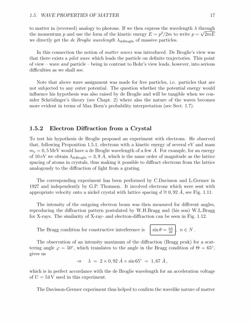
1.5.2 Electron Diffraction from a Crystal

To test his hypothesis de Broglie proposed an experiment with electrons. He observedthat, following Proposition 1.5.1, electrons with a kinetic energy of several eV and massme = 0, 5 MeV would have a de Broglie wavelength of a few A. For example, for an energyof 10 eV we obtain λdeBroglie = 3, 9 A, which is the same order of magnitude as the latticespacing of atoms in crystals, thus making it possible to diffract electrons from the latticeanalogously to the diffraction of light from a grating.

The corresponding experiment has been performed by C.Davisson and L.Germer in1927 and independently by G.P. Thomson. It involved electrons which were sent withappropriate velocity onto a nickel crystal with lattice spacing d ∼= 0, 92 A, see Fig. 1.11.

The intensity of the outgoing electron beam was then measured for different angles,reproducing the diffraction pattern postulated by W.H.Bragg and (his son) W.L.Braggfor X-rays. The similarity of X-ray- and electron-diffraction can be seen in Fig. 1.12.

The Bragg condition for constructive interference is sin θ = nλ2d

, n ∈ N .

The observation of an intensity maximum of the diffraction (Bragg peak) for a scat-tering angle ϕ = 50◦, which translates to the angle in the Bragg condition of Θ = 65◦,gives us

⇒ λ = 2× 0, 92 A× sin 65◦ = 1, 67 A ,

which is in perfect accordance with the de Broglie wavelength for an acceleration voltageof U = 54 V used in this experiment.

The Davisson-Germer experiment thus helped to confirm the wavelike nature of matter


Figure 1.11: Davisson-Germer Experiment: a) An electron beam is diffracted froma nickel crystal and the intensity of the outgoing beam is measured. b) Schemeof the Bragg diffraction from a crystal with lattice spacing d, picture (b) from:http://en.wikipedia.org/wiki/Image:Bragg diffraction.png

and to validate the claims of early quantum mechanics. Davisson and Thomson6 wereawarded the Nobel prize in 1937.

Figure 1.12: Comparison of X-ray- (left) and electron- (right) diffraction patterns causedby the same aperture, namely a small hole in an aluminium foil; pictures from Ref. [2]

6It’s quite amusing that his father J.J. Thomson received the Nobel prize in 1906 for showing the“opposite”, namely that the electron is a particle.

1.6. HEISENBERG’S UNCERTAINTY PRINCIPLE 19

1.6 Heisenberg’s Uncertainty Principle

We now want to introduce a quantum mechanical principle, Heisenberg’s uncertainty prin-ciple that is somehow difficult to grasp conceptually even though the mathematics behindis straightforward. Before we will derive it formally, which we will do in Sect. 2.6, we tryto make it plausible by more heuristic means, namely by the Heisenberg microscope. TheGedankenexperiment of the Heisenberg microscope needs to be seen more as an examplefor the application of the uncertainty principle, than a justification of the principle itself.

1.6.1 Heisenberg’s Microscope

Let’s start by detecting the position of an electron by scattering of light and picturingit on a screen. The electron will then appear as the central dot (intensity maximum)on the screen, surrounded by bright and dark concentric rings (higher order intensitymaxima/minima). Since the electron acts as a light source we have to consider it as anaperture with width d where we know that the condition for destructive interference is

sinφ =nλ

d, n ∈ N . (1.23)

So following Eq. (1.23) the smallest length resolvable by a microscope is given byd = λ/ sinφ and thus the uncertainty of localization of an electron can be written as

∆x = d =λ

sinφ. (1.24)

It seems as if we chose the wavelength λ to be small enough and sinφ to be big, then∆x could become arbitrarily small. But, as we shall see, the accuracy increases at theexpense of the momentum accuracy. Why is that? The photons are detected on thescreen but their direction is unknown within an angle φ resulting in an uncertainty of theelectron’s recoil within an interval ∆. So we can identify the momentum uncertainty (inthe direction of the screen) of the photon with that of the electron

∆pex = ∆pPhoton

x = pPhoton sinφ =h

λsinφ , (1.25)

where we inserted the momentum of the photon pPhoton = ~k = h/λ in the last step.Inserting the position uncertainty of the electron from Eq. (1.24) into Eq. (1.25) we get

Heisenberg’s Uncertainty relation: ∆x∆ px = h

which he received the Nobel prize for in 1932. We will further see in Sect. 2.6 that theaccuracy can be increased by a factor 4π and that the above relation can be generalizedto the statement


∆x∆px ≥ ~2

This is a fundamental principle that has nothing to do with technical imperfections ofthe measurement apparatus. We can phrase the uncertainty principle in the following way:

Proposition 1.6.1Whenever a position measurement is accurate (i.e. precise information aboutthe current position of a particle), the information about the momentum isinaccurate – uncertain – and vice versa.

1.6.2 Energy–Time Uncertainty Principle

We now want to construct another uncertainty relation, the energy–time uncertainty,which describes the relation between the uncertainties ∆t for the time a physical processlasts and ∆E for the respective energy. Consider for example a wave packet travelingalong the x-axis with velocity v. It takes the time ∆t to cover the distance ∆x. We canthus write

energy: E =p2

2m, velocity: v =

∆x

∆t. (1.26)

Calculating the variation ∆E of the energy E and expressing ∆t from the right hand sideof Eq. (1.26) by the velocity v and substituting v = p/m we get

variation: ∆E =p

m∆p, time period: ∆t =

∆x

v=

m

p∆x . (1.27)

The right hand side represents the period of time where the wave is localizable. When wenow multiply ∆t with ∆E we arrive at:

∆t∆E =m

p∆x

p

m∆p = ∆x∆p ≥ ~

2, (1.28)

∆E ∆t ≥ ~2

We can conclude that there is a fundamental complementarity between energy andtime. An important consequence of the energy–time uncertainty is the finite “natural”width of the spectral lines.

1.7 Double–Slit Experiment

1.7.1 Comparison of Classical and Quantum Mechanical Results

We will now take a look at the double–slit experiment, which is well-known from classicaloptics and whose interference pattern is completely understood when considering light

1.7. DOUBLE–SLIT EXPERIMENT 21

as electromagnetic waves. The experiment can be performed with massive particles aswell but then a rather strange phenomenon occurs. It turns out that it is impossible,absolutely impossible, to explain it in a classical way or as Richard Feynman [3] phrasedit emphasizing the great significance of the double–slit as the fundamental phenomenonof quantum mechanics: “ ... the phenomenon [of the double–slit experiment] has in it theheart of quantum mechanics. In reality, it contains the only mystery.”

The associated experiments have been performed with electrons by Mollenstedt andSonsson in 1959 [4], with neutrons by Rauch [5] and Shull [6] in 1969 and by Zeilingeret al. in the eighties [7]. More recently, in 1999 and subsequent years, Arndt et al. [8]performed a series of experiments using large molecules, so-called fullerenes.

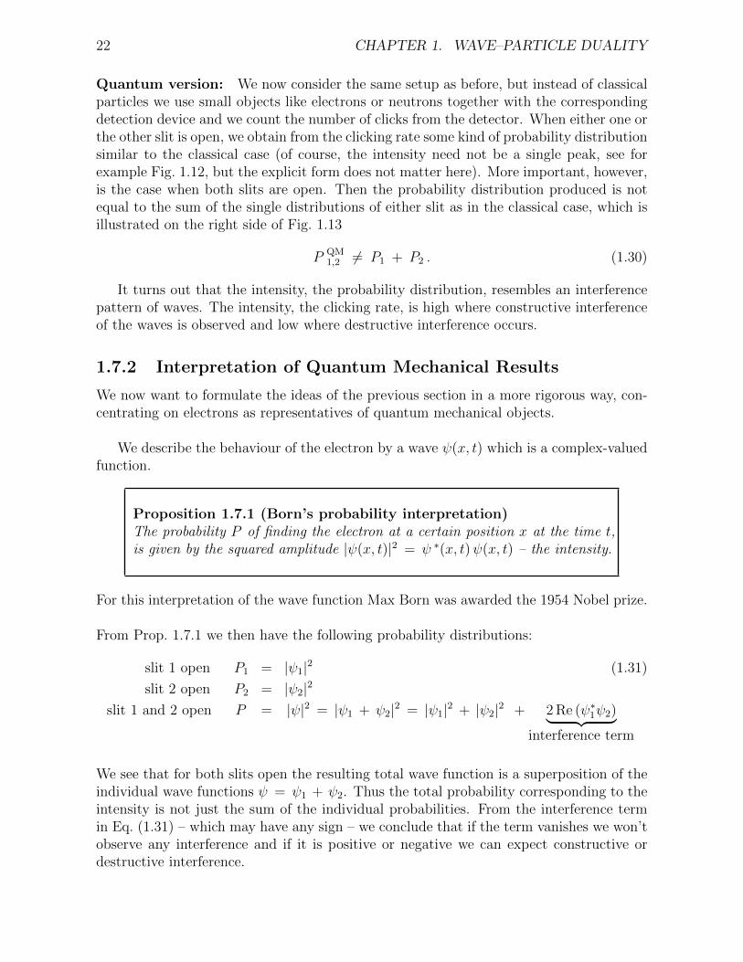
Classical considerations: Let’s consider classical particles that pass through an arrayof two identical slits and are detected on a screen behind the slits. When either the firstslit, the second or both slits are open then we expect a probability distribution to find theparticle on the screen for the third case (both open) to be just the sum of the distributionsfor the first and second case (see left side of Fig. 1.13). We can formally write

P class1,2 = P1 + P2 , (1.29)

where Pk (k = 1, 2) is the distribution when the k-th slit is open. For classical objects,like e.g. marbles, Eq. (1.29) is valid (for accordingly high numbers of objects).

Figure 1.13: Illustration of the double–slit experiment with classical particles (left) andquantum mechanical particles (right); picture used with courtesy of M. Arndt


Quantum version: We now consider the same setup as before, but instead of classicalparticles we use small objects like electrons or neutrons together with the correspondingdetection device and we count the number of clicks from the detector. When either one orthe other slit is open, we obtain from the clicking rate some kind of probability distributionsimilar to the classical case (of course, the intensity need not be a single peak, see forexample Fig. 1.12, but the explicit form does not matter here). More important, however,is the case when both slits are open. Then the probability distribution produced is notequal to the sum of the single distributions of either slit as in the classical case, which isillustrated on the right side of Fig. 1.13

P QM1,2 6= P1 + P2 . (1.30)

It turns out that the intensity, the probability distribution, resembles an interferencepattern of waves. The intensity, the clicking rate, is high where constructive interferenceof the waves is observed and low where destructive interference occurs.

1.7.2 Interpretation of Quantum Mechanical Results

We now want to formulate the ideas of the previous section in a more rigorous way, con-centrating on electrons as representatives of quantum mechanical objects.

We describe the behaviour of the electron by a wave ψ(x, t) which is a complex-valuedfunction.

Proposition 1.7.1 (Born’s probability interpretation)The probability P of finding the electron at a certain position x at the time t,is given by the squared amplitude |ψ(x, t)|2 = ψ ∗(x, t)ψ(x, t) – the intensity.

For this interpretation of the wave function Max Born was awarded the 1954 Nobel prize.

From Prop. 1.7.1 we then have the following probability distributions:

slit 1 open P1 = |ψ1|2 (1.31)

slit 2 open P2 = |ψ2|2

slit 1 and 2 open P = |ψ|2 = |ψ1 + ψ2|2 = |ψ1|2 + |ψ2|2 + 2 Re (ψ∗1ψ2)︸︷︷︸interference term

We see that for both slits open the resulting total wave function is a superposition of theindividual wave functions ψ = ψ1 + ψ2. Thus the total probability corresponding to theintensity is not just the sum of the individual probabilities. From the interference termin Eq. (1.31) – which may have any sign – we conclude that if the term vanishes we won’tobserve any interference and if it is positive or negative we can expect constructive ordestructive interference.


Resume: An electron as a quantum system passes through the double–slit, then hits ascreen or a detector. It produces a very localized lump or causes a click in the detectorthus occurring as a definite particle. But the probability for the detection is given by theintensity |ψ|2 of the wave ψ. It is in this sense that an electron behaves like a particle orlike a wave.

Remark I: The probability distribution – the interference pattern – is not created,as one could deduce, by the simultaneously incoming electrons but does arise throughthe interference of the single electron wave function and thus does not change when theelectrons pass through the double–slit one by one. The spot of a single electron on thescreen occurs totally at random and for few electrons we cannot observe any structure,only when we have gathered plenty of them, say thousands, we can view an interferencepattern, which can be nicely seen in Fig. 1.14.

Figure 1.14: Double–slit experiment with single electrons by Tonomura: The interfer-ence pattern slowly builds up as more and more electrons are sent through the doubleslit one by one; electron numbers are a) 8, b) 270, c) 2000, d) 60000; picture fromhttp://de.wikipedia.org/wiki/Bild:Doubleslitexperiment results Tanamura 1.gif

Remark II: Path measurement If we wish to gain which-way information, i.e. de-termine whether the electron passes slit 1 or 2, e.g. by placing a light–source behind thedouble–slit to illuminate the passing electrons, the interference pattern disappears andwe end up with a classical distribution.


Proposition 1.7.2 (Duality)Gaining path information destroys the wave like behaviour.

It is of crucial importance to recognize that the electron does not split. Whenever anelectron is detected at any position behind the double–slit it is always the whole electronand not part of it. When both slits are open, we do not speak about the electron asfollowing a distinct path since we have no such information7.

1.7.3 Interferometry with C60−Molecules

Small particles like electrons and neutrons are definitely quantum systems and produceinterference patterns, i.e. show a wave-like behaviour. We know from Louis de Broglie’shypothesis that every particle with momentum p can be assigned a wavelength. So it’squite natural to ask how big or how heavy can a particle be in order to keep its interfer-ence ability, what is the boundary, does there exist an upper bound at all ?

This question has been addressed by the experimental group Arndt, Zeilinger et al. [8]in a series of experiments with fullerenes. Fullerenes are C60–molecules with a high spher-ical symmetry, resembling a football with a diameter of approximately D ≈ 1 nm (givenby the outer electron shell) and a mass of 720 amu, see Fig. 1.15.

Figure 1.15: Illustration of the structure of fullerenes: 60 carbon atoms are arranged inpentagonal and hexagonal structures forming a sphere analogously to a football; pictureused with courtesy of M. Arndt

In the experiment fullerenes are heated to about 900 ◦K in an oven from where they areemitted in a thermal velocity distribution. With an appropriate mechanism, e.g. a set of

7Certain interpretations of quantum mechanics might allow one to assign a definite path to an electron,though one would also need to introduce additional parameters which cannot be sufficiently measuredand thus do not improve the predictive power of the theory. For references to the Bohmian interpretationsee for example [9] and [10] and for the many worlds interpretation [11]


constantly rotating slotted disks, a narrow range of velocities is selected from the thermaldistribution. After collimation the fullerenes pass a SiN lattice with gaps of a = 50 nmand a grating period of d = 100 nm and are finally identified with help of an ionizing laserdetector, see Fig. 1.16.

Figure 1.16: Experimental setup for fullerene diffraction; picture by courtesy of M. Arndt

For a velocity vmax = 220 m/s the de Broglie wavelength is

λdeBroglie =h

mv= 2, 5 pm ≈ 1

400D , (1.32)

thus about 400 times smaller than the size of the particle.

As the angle between the central and the first order intensity maximum is very small(thus sin Θ ≈ Θ)

Θ =λdeBroglie

d= 25µrad = 5” (1.33)

a good collimation is needed to increase the spatial (transverse) coherence. The wholeexperiment also has to be performed in a high vacuum chamber, pictured in Fig. 1.17, toprevent decoherence of the fullerene waves by collision with residual gas molecules.

The fullerenes are ionized by a laser beam in order to simplify the detection process,where an ion counter scans the target area, see Fig. 1.16.

We can also conclude that the fullerenes do not interfere with each other due to theirhigh temperature, i.e. they are in high modes of vibration and rotation, thus occurring asclassically distinguishable objects. Even so to prevent collisions the intensity of the beamis kept very low to ensure a mean distance of the single fullerenes of some mm (whichis about 1000 times further than the intermolecular potentials reach). As a side effectof the high temperature the fullerenes emit photons8 (black body radiation) but, fortu-nately, these photons don’t influence the interference pattern because their wavelengthsλ ≈ 5− 20µm are much bigger than the grating period (the double–slit). Thus we don’tget any path information and the interference phenomenon remains.

8The probality for photon emission is rather small for the 900 K mentioned, for temperatures higherthan 1500 K the probability of emitting (visible) photons is considerably higher but their effects can beneglected for the setup we have described here.


Figure 1.17: Photography of the experimental setup; picture by courtesy of M. Arndt

Looking finally at the result of the fullerene interferometry in Fig. 1.18 we see thatthe detection counts do very accurately fit the diffraction pattern9 of the grating, thusdemonstrating nicely that quite massive particles behave as true quantum systems.10

Figure 1.18: Results of the fullerene experiments, see [12]; picture by courtesy of M. Arndt

9The inquisitive reader might have noticed that for a grating with a 100 nm period and 50 nm wideslits, the second order diffraction maximum shouldn’t exist at all, since the first order minimum of thesingle slit should cancel the second order maximum of the grating. The reason for its existence lies in theeffective reduction of the slit width by Van-der-Waals interaction.

10It’s quite amusing to notice, while the mass of a fullerene, also called bucky ball, does not agree withthe requirements for footballs the symmetry and shape actually does, and furthermore the ratio betweenthe diameter of a buckyball (1 nm) and the width of the diffraction grating slits (50 nm) compares quitewell with the ratio between the diameter of a football (22 cm) and the width of the goal (732 cm).

chapter 1 wave{particle duality -...

Documents