chapter 1 signal and systems

ELG 3120 Signals and Systems Chapter 1

1/1 Yao

Chapter 1 Signal and Systems

1.1 Continuous-time and discrete-time Signals

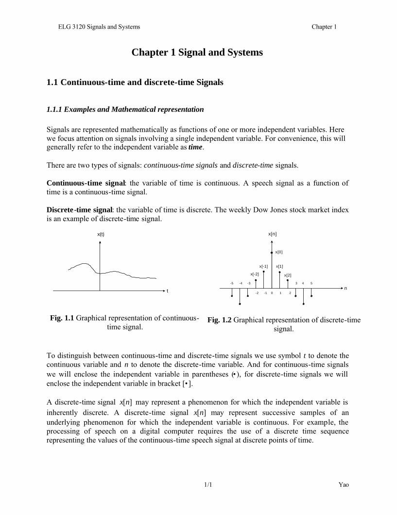
1.1.1 Examples and Mathematical representation Signals are represented mathematically as functions of one or more independent variables. Here we focus attention on signals involving a single independent variable. For convenience, this will generally refer to the independent variable as time. There are two types of signals: continuous-time signals and discrete-time signals. Continuous-time signal: the variable of time is continuous. A speech signal as a function of time is a continuous-time signal. Discrete-time signal: the variable of time is discrete. The weekly Dow Jones stock market index is an example of discrete-time signal.

To distinguish between continuous-time and discrete-time signals we use symbol t to denote the continuous variable and n to denote the discrete-time variable. And for continuous-time signals we will enclose the independent variable in parentheses (•), for discrete-time signals we will enclose the independent variable in bracket [•]. A discrete-time signal ][nx may represent a phenomenon for which the independent variable is inherently discrete. A discrete-time signal ][nx may represent successive samples of an underlying phenomenon for which the independent variable is continuous. For example, the processing of speech on a digital computer requires the use of a discrete time sequence representing the values of the continuous-time speech signal at discrete points of time.

t

x(t)

Fig. 1.1 Graphical representation of continuous-time signal.

n

x[n]

x[0]

x[1]

x[2]

x[-1]

x[-2]

0 1 2

3 4 5

-1-2

-3-4-5

Fig. 1.2 Graphical representation of discrete-time signal.


2/1 Yao

1.1.2 Signal Energy and Power If )(tv and )(ti are respectively the voltage and current across a resistor with resistance R , then the instantaneous power is

)(1)()()( 2 tvR

titvtp == . (1.1)

The total energy expended over the time interval 21 ttt ≤≤ is

∫∫ = 2

1

2

1

)(1)( 2t

t

t

tdttv

Rdttp , (1.2)

and the average power over this time interval is

∫∫ −=

−2

1

2

1

)(11)(1 2

1212

t

t

t

tdttv

Rttdttp

tt. (1.3)

For any continuous-time signal )(tx or any discrete-time signal ][nx , the total energy over the time interval 21 ttt ≤≤ in a continuous-time signal )(tx is defined as

∫2

1

2)(t

tdttx , (1.4)

where x denotes the magnitude of the (possibly complex) number x . The time-averaged power

is ∫−2

1

2

12

)(1 t

tdttx

tt. Similarly the total energy in a discrete-time signal ][nx over the time

interval 21 nnn ≤≤ is defined as

∑2

1

2][n

n

nx (1.5)

The average power is ∑+−

2

1

2

12

][1

1 n

n

nxnn

In many systems, we will be interested in examining the power and energy in signals over an infinite time interval, that is, for +∞≤≤∞− t or +∞≤≤∞− n . The total energy in continuous time is then defined

dttxdttxET

TT

22)()(lim ∫∫

∞

∞−−∞→∞ == , (1.6)


3/1 Yao

and in discrete time

∑∑+∞

∞−

+

−∞→∞ ==

22 ][][lim nxnxEN

NN

. (1.7)

For some signals, the integral in Eq. (1.6) or sum in Eq. (1.7) might not converge, that is, if )(tx or ][nx equals a nonzero constant value for all time. Such signals have infinite energy, while signals with ∞<∞E have finite energy. The time-averaged power over an infinite interval

dttxT

PT

TT

2)(

21lim ∫−∞→∞ = (1.8)

∑+

−∞→∞ +

=N

NN

nxN

P2][

121lim (1.9)

Three classes of signals: • Class 1: signals with finite total energy, ∞<∞E and zero average power,

02

lim == ∞

∞→∞ TE

PT

(1.10)

• Class 2: with finite average power ∞P . If 0>∞P , then ∞=∞E . An example is the signal

4][ =nx , it has infinite energy, but has an average power of ∞P =16. Class 3: signals for which neither ∞P and ∞E are finite. An example of this signal is ttx =)( .

1.2 Transformations of the independent variable In many situations, it is important to consider signals related by a modification of the independent variable. These modifications will usually lead to reflection, scaling, and shift.

1.2.1 Examples of Transformations of the Independent Variable

J-P Yao

Text Box

(Energy Signal)

J-P Yao

Text Box

(Power Signal)


4/1 Yao

n

x[n]

n

x[n-n0]

n0

(a) (b)

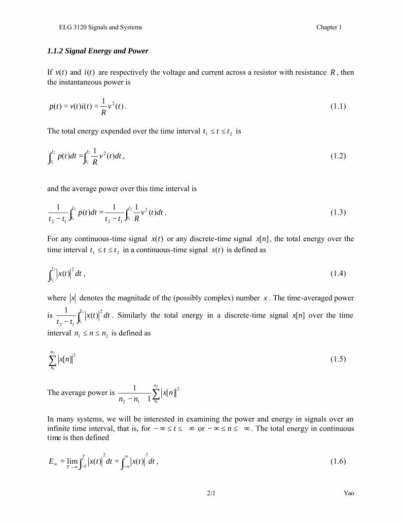
Fig.1.3 Discrete-time signals related by a time shift.

t

x(t)

t

x(t-t0)

t0

Fig. 1.4 Continuous-time signals related by a time shift.

n

x[n]

n

x[-n]

(a) (b)

Fig. 1.5 (a) A discrete-time signal ][nx ; (b) its reflection, ][ nx − about 0=n .

t

x(t)

0

t

x(-t)

0

(a) (b)

Fig. 1.6 (a) A continuous-time signal )(tx ; (b) its reflection, )( tx − about 0=t .


5/1 Yao

x(t)

tt

x(2t)

0 (a) (b)

x(t/2)

0t

(c)

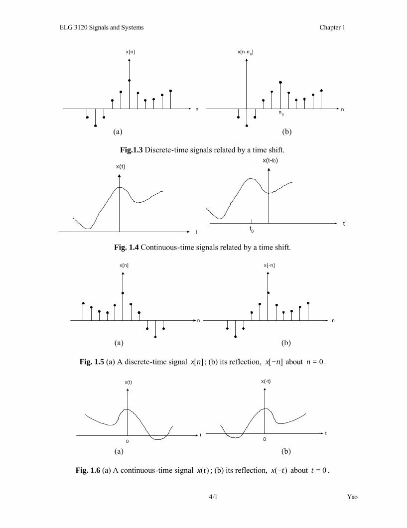
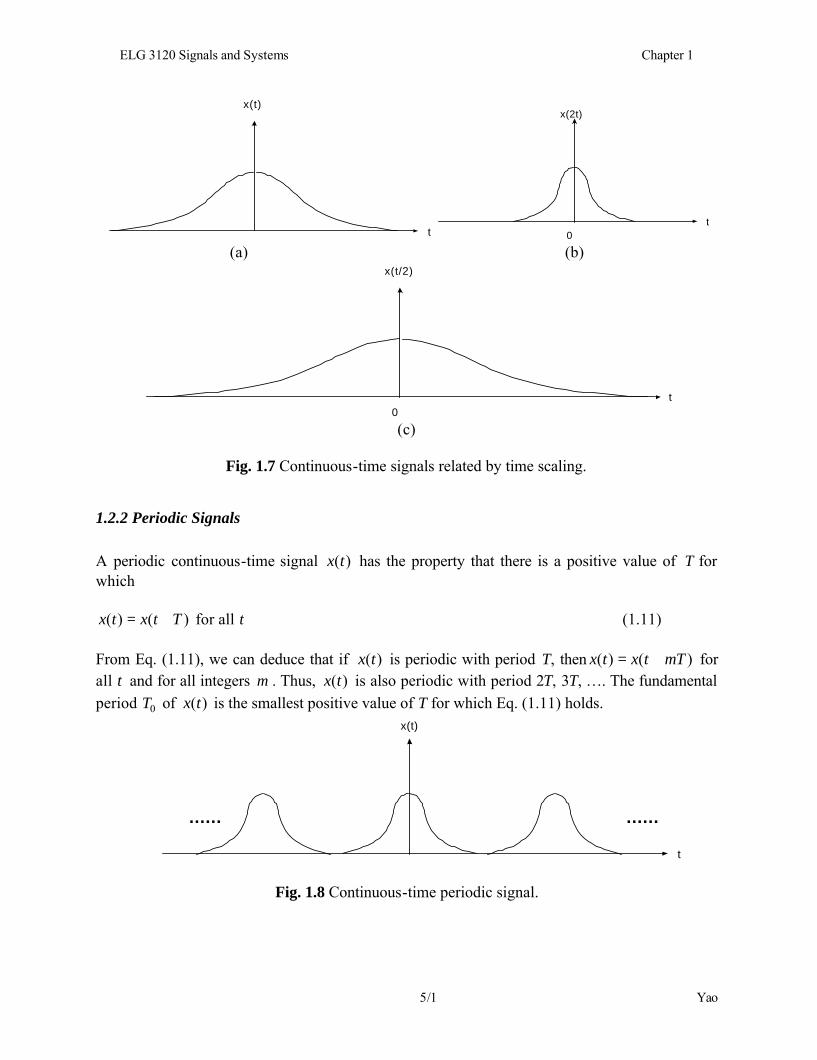
Fig. 1.7 Continuous-time signals related by time scaling.

1.2.2 Periodic Signals

A periodic continuous-time signal )(tx has the property that there is a positive value of T for which

)()( Ttxtx += for all t (1.11)

From Eq. (1.11), we can deduce that if )(tx is periodic with period T, then )()( mTtxtx += for all t and for all integers m . Thus, )(tx is also periodic with period 2T, 3T, …. The fundamental period 0T of )(tx is the smallest positive value of T for which Eq. (1.11) holds.

t

x(t)

............

Fig. 1.8 Continuous-time periodic signal.


6/1 Yao

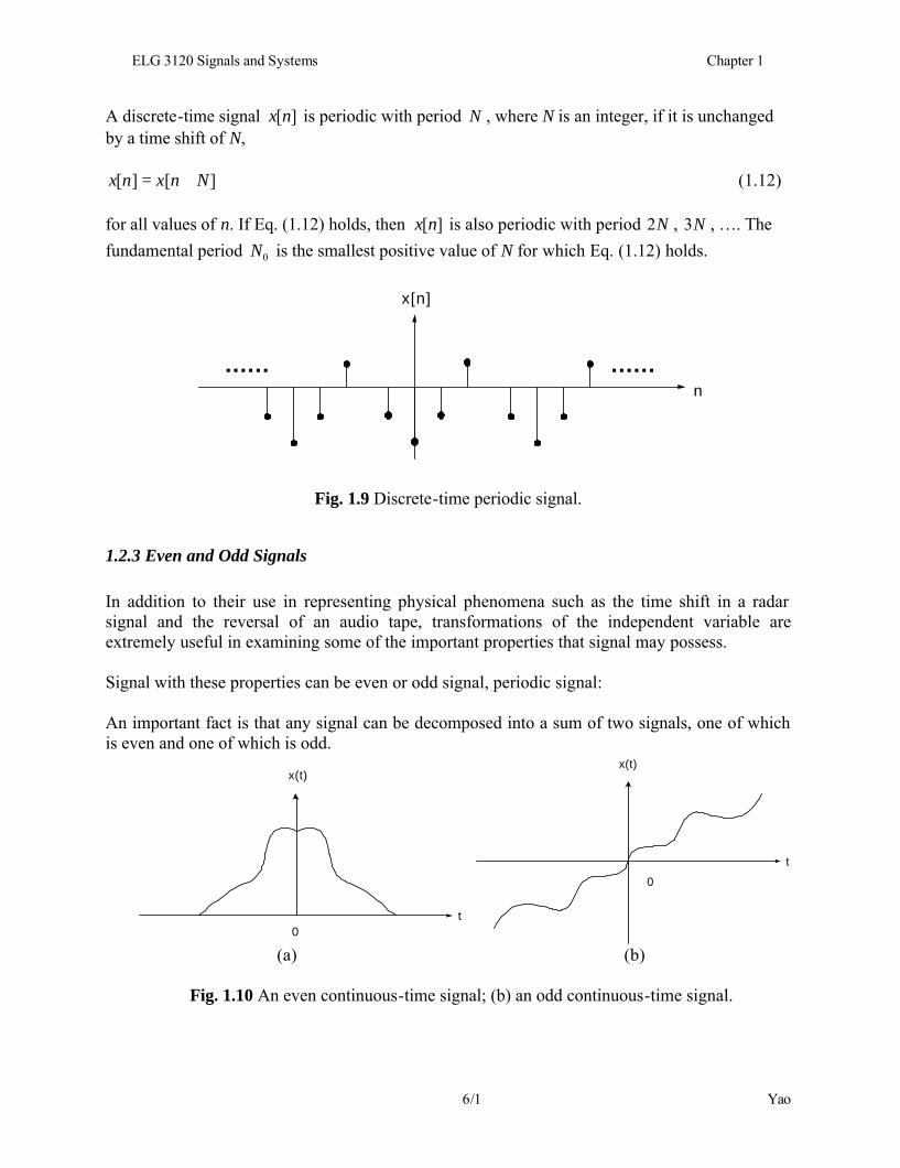
A discrete-time signal ][nx is periodic with period N , where N is an integer, if it is unchanged by a time shift of N,

][][ Nnxnx += (1.12)

for all values of n. If Eq. (1.12) holds, then ][nx is also periodic with period N2 , N3 , …. The fundamental period 0N is the smallest positive value of N for which Eq. (1.12) holds.

n

x[n]

............

Fig. 1.9 Discrete-time periodic signal.

1.2.3 Even and Odd Signals

In addition to their use in representing physical phenomena such as the time shift in a radar signal and the reversal of an audio tape, transformations of the independent variable are extremely useful in examining some of the important properties that signal may possess. Signal with these properties can be even or odd signal, periodic signal: An important fact is that any signal can be decomposed into a sum of two signals, one of which is even and one of which is odd.

t

x(t)

0

t

x(t)

0

(a) (b)

Fig. 1.10 An even continuous-time signal; (b) an odd continuous-time signal.


7/1 Yao

{ } [ ])()(21)( txtxtxEV −+= (1.13)

which is referred to as the even part of )(tx . Similarly, the odd part of )(tx is given by

{ } [ ])()(21)( txtxtxOD −−= (1.14)

Exactly analogous definitions hold in the discrete-time case.

n

x[n]

1

<≥

=0,00,1

][nn

nx

n

x[n]

1

21

{ }

>

=

<

=

0,21

0,1

0,21

][

n

n

n

nxEV

(a) (b)

n

x[n]

21

21

−

{ }

>

=

<−

=

0,21

0,0

0,21

][

n

n

n

nxOD

(c)

Fig.1.11 The even-odd decomposition of a discrete-time signal.

1.3 Exponential and sinusoidal signals

1.3.1 Continuous-time complex exponential and sinusoidal signals The continuous-time complex exponential signal

atCetx =)( (1. 15) where C and a are in general complex numbers.


8/1 Yao

Real exponential signals

t

x(t)

C

t

x(t)

C

(a) (b)

Fig. 1.12 The continuous-time complex exponential signal atCetx =)( , (a) 0>a ; (b) 0<a . Periodic complex exponential and sinusoidal signals If a is purely imaginary, we have

tjetx 0)( ω= (1.16) An important property of this signal is that it is periodic. We know )(tx is periodic with period T if

TjtjTtjtj eeee 0000 )( ωω+ωω == (1.17) For periodicity, we must have

10 =ω Tje (1.18) For 00 ≠ω , the fundamental period 0T is

00

2ω

π=T (1.19)

Thus, the signals tje 0ω and tje 0ω− have the same fundamental period. A signal closely related to the periodic complex exponential is the sinusoidal signal

)cos()( 0 φ+ω= tAtx (1.20) With seconds as the unit of t, the units of φ and 0ω are radians and radians per second. It is also known 00 2 fπω = , where 0f has the unit of circles per second or Hz.


9/1 Yao

The sinusoidal signal is also a periodic signal with a fundamental period of 0T .

00

2ω

π=T

A

)cos()( 0 φω += tAtx

φcosA

t

Fig. 1.13 Continuous-time sinusoidal signal.

Using Euler’s relation, a complex exponential can be expressed in terms of sinusoidal signals with the same fundamental period:

tjte tj00 sincos0 ωωω += (1.21)

Similarly, a sinusoidal signal can also be expressed in terms of periodic complex exponentials with the same fundamental period:

tjjtjj eeA

eeA

tA 00

22)cos( 0

ωφωφφω −−+=+ (1.22)

A sinusoid can also be expresses as

{ })(0

0Re)cos( φωφω +=+ tjeAtA (1.23) and

{ })(0

0Im)sin( φωφω +=+ tjeAtA (1.24) Periodic signals, such as the sinusoidal signals provide important examples of signal with infinite total energy, but finite average power. For example:

∫∫ === 000

0 001

TT tjperiod TdtdteE ω (1.25)

∫∫ === 00 0

000

111 TT tjperiod dtdte

TP ω (1.26)


10/1 Yao

Since there are an infinite number of periods as t ranges from ∞− to ∞+ , the total energy integrated over all time is infinite. The average power is finite since

121lim

20 == ∫−∞→∞ dte

TP

T

T

tj

T

ω (1.27)

Harmonically related complex exponentials:

tjkk et 0)( ωφ = , ......,2,1,0 ±±=k (1.28)

0ω is the fundamental frequency.

Example: Signal tjtj eetx 32)( += can be expressed as )5.0cos(2)()( 5.25.05.05.2 teeeetx tjtjtjtj =+= − , the magnitude of )(tx is )5.0cos(2)( ttx = , which is commonly referred to as a full-wave rectified sinusoid, shown in Fig. 1.14.

t0

2

)(tx

π2 π4π− 2π− 4

Fig. 1.14 Full-wave rectified sinusoid. General complex Exponential signals Consider a complex exponential atCe , where θjeCC = is expressed in polar and 0ωjra += is expressed in rectangular form. Then

)sin()cos( 00)()( 00 θωθωθωωθ +++=== ++ teCjteCeeCeeCCe rtrttjrttjrjat . (1.29)

Thus, for 0=r , the real and imaginary parts of a complex exponential are sinusoidal. For 0>r , sinusoidal signals multiplied by a growing exponential. For 0<r , sinusoidal signals multiplied by a decaying exponential. Damped signal – Sinusoidal signals multiplied by decaying exponentials are commonly refereed to as damped signal.


11/1 Yao

t

x(t)

t

x(t)

(a) (b)

Fig. 1.15 (a) Growing sinusoidal signal; (b) decaying sinusoidal signal.

1.3.2 Discrete-time complex exponential and sinusoidal signals A discrete complex exponential or sequence is defined by

nCnx α=][ , (1.30) where C and α are in general complex numbers. This can be alternatively expressed

nCenx β=][ , (1.31)

where βα e= . Real Exponential Signals If C and α are real, we have the real exponential signals.

x[n]

n

x[n]

n

(a) (b)

x[n]

n

x[n]

n

(c) (d)


12/1 Yao

Fig. 1.16 Real Exponential Signal nCnx α=][ : (a) α >1; (b) 0<α <1; (c) –1<α <0; (d) α <-1.

Sinusoidal Signals

njenx 0][ ω= (1.32)

njne nj00 sincos0 ω+ω=ω (1.33)

Similarly, a sinusoidal signal can also be expresses in terms of periodic complex exponentials with the same fundamental period:

njjnjj eeA

eeA

nA 00

22)cos( 0

ω−φ−ωφ +=φ+ω (1.34)

A sinusoid can also be expresses as

{ })(0

0Re)cos( φ+ω=φ+ω njeAnA (1.35) and

{ })(0

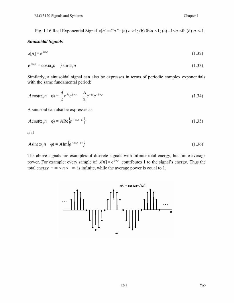
0Im)sin( φ+ω=φ+ω njeAnA (1.36) The above signals are examples of discrete signals with infinite total energy, but finite average power. For example: every sample of njenx 0][ ω= contributes 1 to the signal’s energy. Thus the total energy +∞<<∞− n is infinite, while the average power is equal to 1.


13/1 Yao

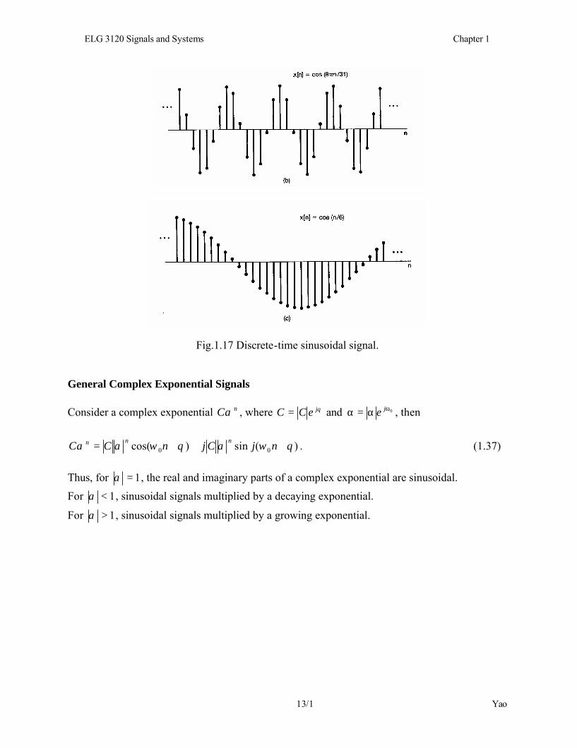
Fig.1.17 Discrete-time sinusoidal signal.

General Complex Exponential Signals Consider a complex exponential nCα , where θjeCC = and 0ωα=α je , then

)(sin)cos( 00 θωαθωαα +++= njCjnCC nnn . (1.37) Thus, for 1=α , the real and imaginary parts of a complex exponential are sinusoidal.

For 1<α , sinusoidal signals multiplied by a decaying exponential.

For 1>α , sinusoidal signals multiplied by a growing exponential.


14/1 Yao

(a) (b)

Fig. 1.18 (a) Growing sinusoidal signal; (b) decaying sinusoidal signal.

1.3.3 Periodicity Properties of Discrete-Time Complex Exponentials There are a number of important differences between continuous-time and discrete-time sinusoidal signals. The continuous-time signals tje 0ω are distinct for distinct values of 0ω . For discrete-time signals, however, these values are not distinct because the signal with 0ω is identical to the signals with frequencies πω 20 ± , πω 40 ± , and so on,

njnjnj eee 000 )4()2( ωπωπω == ±± . (1.38) In considering discrete-time exponentials, we need only consider a frequency interval of π2 . In most occasions, we will use the interval πω 20 0 <≤ or πωπ <≤− 0 . The discrete-time signal njenx 0][ ω= does not have a continuously increasing rate of oscillation as 0ω is increased in magnitude, but as 0ω is increased from 0, the signal oscillates more and more rapidly until 0ω reaches π , and when 0ω is continuously increased, the rate of oscillation


15/1 Yao

decreases until 0ω reaches π2 . We conclude that the low-frequency discrete-time exponentials have values of 0ω near 0, π2 , and any other even multiple of π , while the high-frequencies are located near πω ±=0 and other odd multiples of π . In order for the signal njenx 0][ ω= to be periodic with period 0>N , we must have

njNnj ee 00 )( ωω =+ , (1.39) or equivalently

10 =Nje ω . (1.40) For Eq. (1.40) to hold, N0ω must be a multiple of π2 . That is, there must be an integer m such that

mN πω 20 = , (1.41) or equivalently

Nm=

πω2

0 . (1.42)

From Eq. (1.40), njenx 0][ ω= is a periodic if πω 2/0 is a rational number and is not periodic otherwise. The fundamental frequency of the discrete-time signal njenx 0][ ω= is

mN02 ωπ = , (1.43)

and the fundamental period of the signal can be

=

0

2ω

πmN . (1.44)

The comparison of the continuous-time and discrete-time signals are summarized in the table below:


16/1 Yao

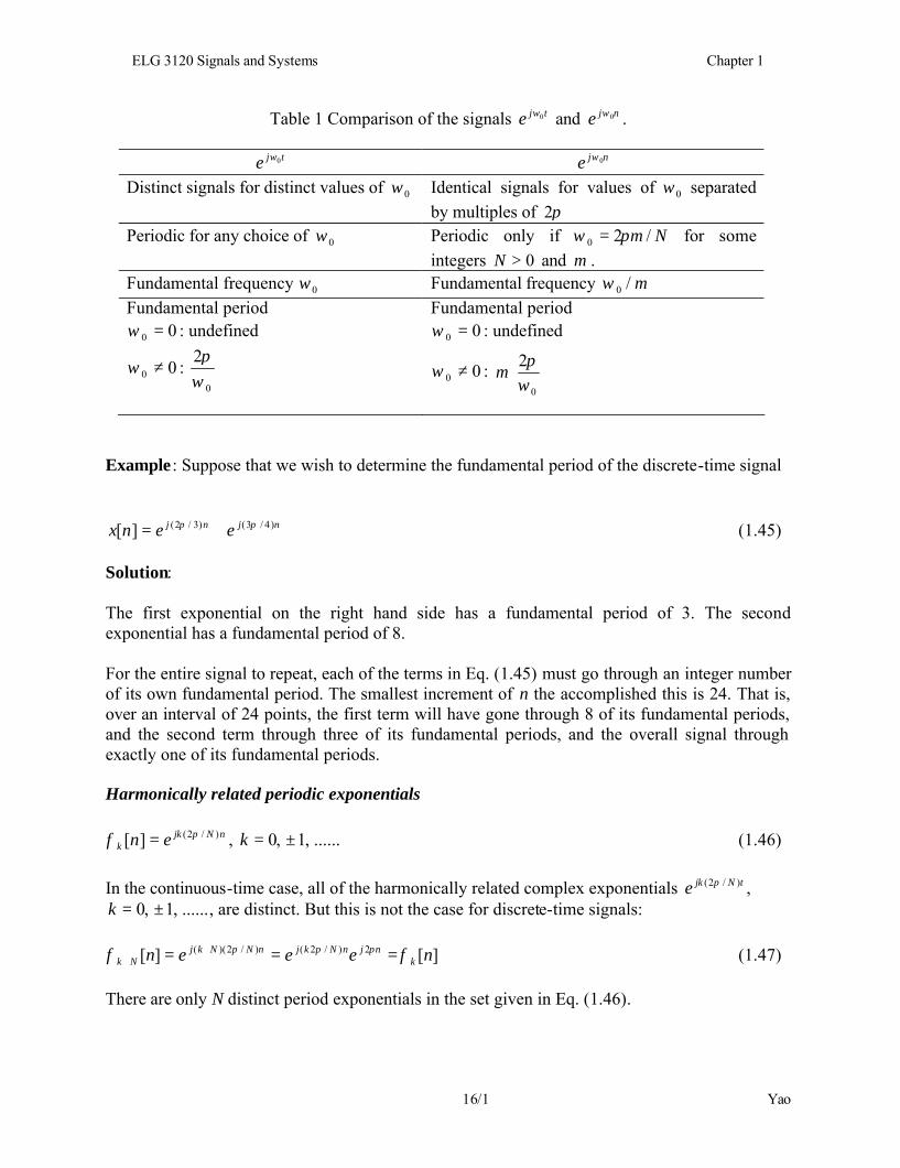
Table 1 Comparison of the signals tje 0ω and nje 0ω .

tje 0ω nje 0ω Distinct signals for distinct values of 0ω Identical signals for values of 0ω separated

by multiples of π2 Periodic for any choice of 0ω Periodic only if Nm /20 πω = for some

integers 0>N and m . Fundamental frequency 0ω Fundamental frequency m/0ω Fundamental period

00 =ω : undefined

00 ≠ω : 0

2ω

π

Fundamental period 00 =ω : undefined

00 ≠ω :

0

2ω

πm

Example : Suppose that we wish to determine the fundamental period of the discrete-time signal

njnj eenx )4/3()3/2(][ ππ += (1.45) Solution: The first exponential on the right hand side has a fundamental period of 3. The second exponential has a fundamental period of 8. For the entire signal to repeat, each of the terms in Eq. (1.45) must go through an integer number of its own fundamental period. The smallest increment of n the accomplished this is 24. That is, over an interval of 24 points, the first term will have gone through 8 of its fundamental periods, and the second term through three of its fundamental periods, and the overall signal through exactly one of its fundamental periods. Harmonically related periodic exponentials

nNjkk en )/2(][ πφ = , ......,1,0 ±=k (1.46)

In the continuous-time case, all of the harmonically related complex exponentials tNjke )/2( π ,

......,1,0 ±=k , are distinct. But this is not the case for discrete-time signals:

][][ 2)/2()/2)(( neeen knjnNkjnNNkj

Nk φφ πππ === ++ (1.47)

There are only N distinct period exponentials in the set given in Eq. (1.46).


17/1 Yao

1.4 The Unit Impulse and Unit Step Functions The unit impulse and unit step functions in continuous and discrete time are considerably important in signal and system analysis.

1.4.1 The discrete-Time Unit Impulse and Unit Step Sequences Discrete-time unit impulse is defined as

=≠

=0,10,0

][nn

nδ , (1.48)

n

][nδ

Fig. 1.19 Discrete-time unit impulse.

Discrete-time unit step is defined as

≥<

=0,10,0

][nn

nu , (1.49)

n

][nu

1

0

Fig. 1.20 Discrete-time unit step sequence. The discrete-time impulse unit is the first difference of the discrete-time step

]1[][][ −−= nununδ , (1.50) The discrete-time unit step is the running sum of the unit sample:


18/1 Yao

∑−∞=

=n

m

mnu ][][ δ , (1.51)

It can be seen that for 0<n , the running sum is zero, and for 0≥n , the running sum is 1.

If we change the variable of summation from m to mnk −= we have, ∑∞

=

−=0

][][k

knnu δ .

The unit impulse sequence can be used to sample the value of a signal at 0=n . Since ][nδ is nonzero only for 0=n , it follows that

][]0[][][ nxnnx δδ = . (1.52) More generally, a unit impulse ][ 0nn −δ , then

][][][][ 000 nnnxnnnx −=− δδ (1.53) This sampling property is very important in signal analysis.

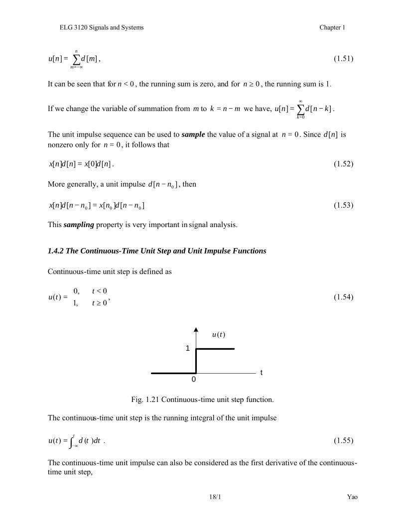
1.4.2 The Continuous-Time Unit Step and Unit Impulse Functions Continuous-time unit step is defined as

≥<

=0,10,0

)(tt

tu , (1.54)

t

)(tu

1

0

Fig. 1.21 Continuous-time unit step function. The continuous-time unit step is the running integral of the unit impulse

∫ ∞−=

tdtu ττδ )()( . (1.55)

The continuous-time unit impulse can also be considered as the first derivative of the continuous-time unit step,


19/1 Yao

dttdu

t)()( =δ . (1.56)

Since )(tu is discontinuous at 0=t and consequently is formally not differentiable. This can be interpreted, however, by considering an approximation to the unit step )(tu ∆ , as illustrated in the figure below, which rises from the value of 0 to the value 1 in a short time interval of length ∆ .

)(tu ∆

1

∆0t

∆0

∆

1

t

)(t∆δ

(a) (b)

Fig. 1.22 (a) Continuous approximation to the unit step )(tu ∆ ; (b) Derivative of )(tu ∆ .

The derivative is

dttdu

t)()( ∆

∆ =δ , (1.57)

∆<≤

∆=∆

otherwise

tt,0

0,1)(δ , (1.58)

as shown in Fig. 1.22. Note that )(t∆δ is a short pulse, of duration ∆ and with unit area for any value of ∆ . As 0→∆ ,

)(t∆δ becomes narrower and higher, maintaining its unit area. At the limit,

)(lim)(0

tt ∆→∆= δδ , (1.59)

)(lim)(

0tutu ∆→∆

= , (1.60)

and


20/1 Yao

dttdu

t)()( =δ . (1.61)

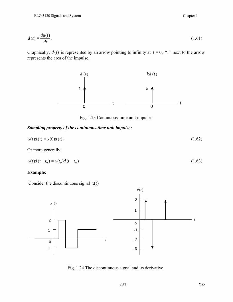
Graphically, )(tδ is represented by an arrow pointing to infinity at 0=t , “1” next to the arrow represents the area of the impulse.

t

)(tδ

1

0t

)(tkδ

k

0

Fig. 1.23 Continuous-time unit impulse. Sampling property of the continuous-time unit impulse:

)()0()()( txttx δδ = , (1.62) Or more generally,

)()()()( 000 tttxtttx −=− δδ (1.63) Example: Consider the discontinuous signal )(tx

)(tx

2

0t

-1

1

2

-3

t

1

-1

-2

)(tx&

0

Fig. 1.24 The discontinuous signal and its derivative.


21/1 Yao

Note that the derivative of a unit step with a discontinuity of size of k gives rise to an impulse of area k at the point of discontinuity.

1.5 Continuous-Time and Discrete-Time Systems A system can be viewed as a process in which input signals are transformed by the system or cause the system to respond in some way, resulting in other signals as outputs. Examples

+-

R

C)(tvs )(0 tv

+

-)(ti

(a)

)(tf

(b)

Fig. 1. 25 Examples of systems. (a) A system with input voltage )(tvs and output voltage )(0 tv .

(b) A system with input equal to the force )(tf and output equal to the velocity )(tv .

A continuous-time system is a system in which continuous-time input signals are applied and results in continuous-time output signals.

Continuous-timesystem

)(tx )(ty

A discrete-time system is a system in which discrete-time input signals are applied and results in discrete-time output signals.

Discrete-timesystem

][nx ][ny


22/1 Yao

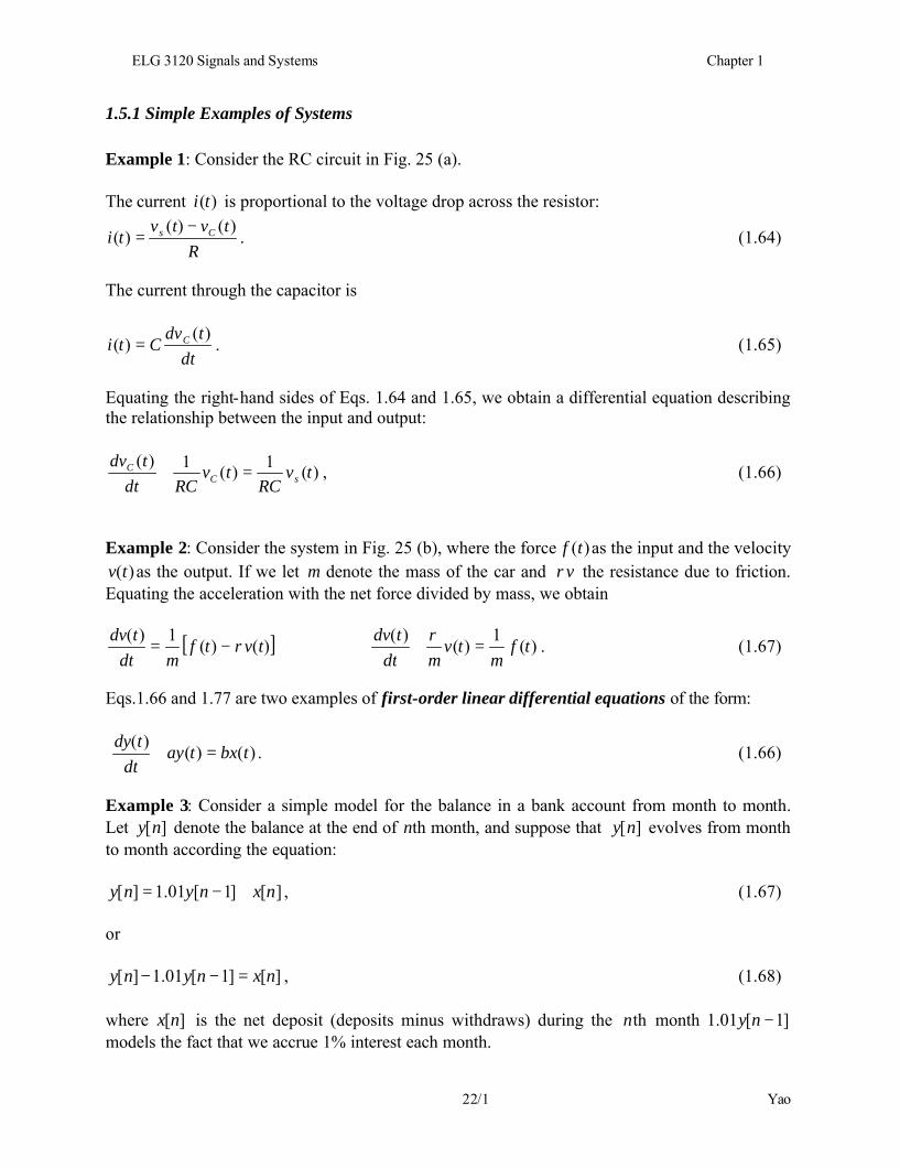
1.5.1 Simple Examples of Systems Example 1: Consider the RC circuit in Fig. 25 (a). The current )(ti is proportional to the voltage drop across the resistor:

Rtvtv

ti Cs )()()( −= . (1.64)

The current through the capacitor is

dttdv

Cti C )()( = . (1.65)

Equating the right-hand sides of Eqs. 1.64 and 1.65, we obtain a differential equation describing the relationship between the input and output:

)(1)(1)(tv

RCtv

RCdttdv

sCC =+ , (1.66)

Example 2: Consider the system in Fig. 25 (b), where the force )(tf as the input and the velocity

)(tv as the output. If we let m denote the mass of the car and vρ the resistance due to friction. Equating the acceleration with the net force divided by mass, we obtain

[ ])()(1)(tvtf

mdttdv

ρ−= ⇒ )(1)()(tf

mtv

mdttdv

=+ρ . (1.67)

Eqs.1.66 and 1.77 are two examples of first-order linear differential equations of the form:

)()()(tbxtay

dttdy

=+ . (1.66)

Example 3: Consider a simple model for the balance in a bank account from month to month. Let ][ny denote the balance at the end of nth month, and suppose that ][ny evolves from month to month according the equation:

][]1[01.1][ nxnyny +−= , (1.67) or

][]1[01.1][ nxnyny =−− , (1.68) where ][nx is the net deposit (deposits minus withdraws) during the nth month ]1[01.1 −ny models the fact that we accrue 1% interest each month.


23/1 Yao

Example 4: Consider a simple digital simulation of the differential equation in Eq. (1.67), in which we resolve time into discrete intervals of length ∆ and approximate )(/)( tdtdv at ∆= nt by the first backward difference, i.e.,

∆∆−−∆ ))1(()( nvnv

Let )(][ ∆= nvnv and )(][ ∆= nfnf , we obtain the following discrete-time model relating the sampled signals ][nv and ][nf ,

][)(

]1[)(

][ nfm∆

nvm

mnv

∆+=−

∆+−

ρρ. (1.69)

Comparing Eqs. 1.68 and 1.69, we see that they are two examples of the first-order linear difference equation, that is,

][]1[][ nbxnayny =−+ . (1.70)

Some conclusions:

• Mathematical descriptions of systems have great deal in common;• A particular class of systems is referred to as linear, time-invariant systems.• Any model used in describing and analyzing a physical system represents an idealization of

the system.

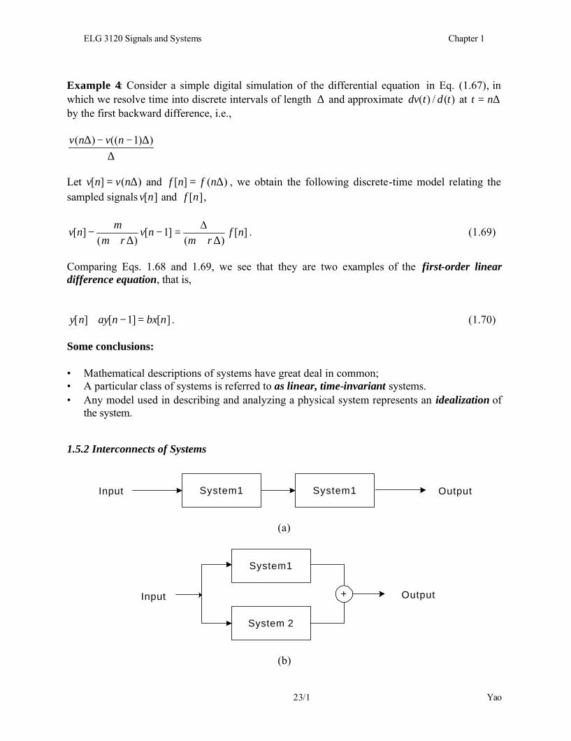
1.5.2 Interconnects of Systems

System1 System1Input Output

(a)

System1

System 2

+Input Output

(b)


24/1 Yao

System1

System 3

Input Output+

System 2

(c)

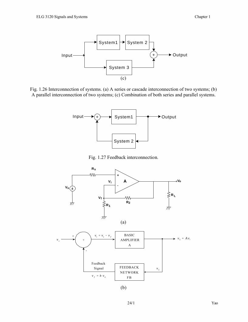
Fig. 1.26 Interconnection of systems. (a) A series or cascade interconnection of two systems; (b) A parallel interconnection of two systems; (c) Combination of both series and parallel systems.

System1Input Output

System 2

+

Fig. 1.27 Feedback interconnection.

V ±

Rs

Vi

s

+

-A

R1R2

VfR L

Vo

•

(a)

FB

BASICAMPLIFIER

A

FEEDBACKNETWORK

++

-

sv

FeedbackSignal

Lf vv β=

Lv

iL vAv =fsi vvv −=

(b)


25/1 Yao

Fig. 1.28 A feedback electrical amplifier.

1.6 Basic System Properties

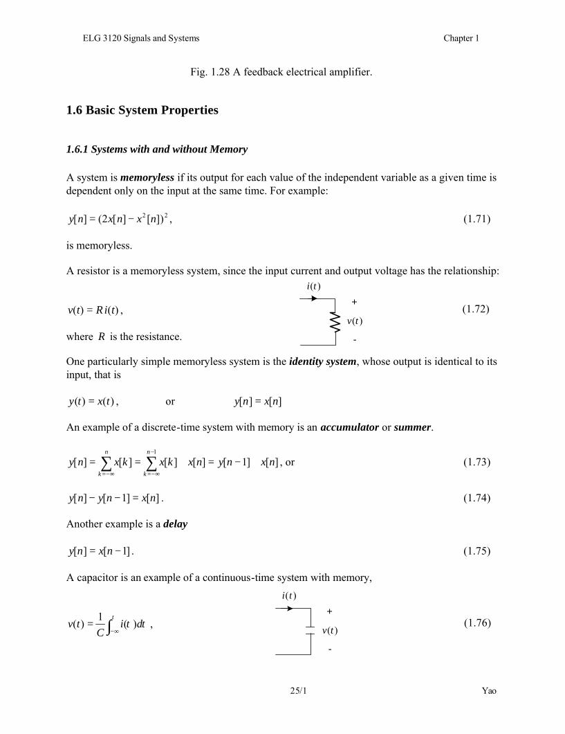
1.6.1 Systems with and without Memory A system is memoryless if its output for each value of the independent variable as a given time is dependent only on the input at the same time. For example:

22 ])[][2(][ nxnxny −= , (1.71) is memoryless. A resistor is a memoryless system, since the input current and output voltage has the relationship:

)()( tiRtv = , (1.72) where R is the resistance. One particularly simple memoryless system is the identity system, whose output is identical to its input, that is

)()( txty = , or ][][ nxny = An example of a discrete-time system with memory is an accumulator or summer.

][]1[][][][][1

nxnynxkxkxnyn

k

n

k

+−=+== ∑∑−

−∞=−∞=

, or (1.73)

][]1[][ nxnyny =−− . (1.74)

Another example is a delay

]1[][ −= nxny . (1.75) A capacitor is an example of a continuous-time system with memory,

ττ∫ ∞−=

tdi

Ctv )(1)( , (1.76)

+

-

)(tv

)(ti

+

-

)(tv

)(ti


26/1 Yao

where C is the capacitance.

1.6.2 Invertibility and Inverse System A system is said to be invertible if distinct inputs leads to distinct outputs.

Systemx[n]y[n]

w[n]=x[n]Inversesystem

y(t)=2x(t)x(t)y(t)

w(t)=x(t)w(t)=0.5y(t)

x[n]y(t)

∑− ∞=

=n

k

kxny ][][ ]1[][][ −−= nynynw ][][ nxnw =

Fig. 1.29 Concept of an inverse system.

Examples of non-invertible systems:

0][ =ny , the system produces zero output sequence for any input sequence.

)()( 2 txty = , in which case, one cannot determine the sign of the input from the knowledge of the output. Encoder in communication systems is an example of invertible system, that is, the input to the encoder must be exactly recoverable from the output.

1.6.3 Causality A system is causal if the output at any time depends only on the values of the input at present time and in the past. Such a system is often referred to as being nonanticipative, as the system output does not anticipate future values of the input. The RC circuit in Fig. 25 (a) is causal, since the capacitor voltage responds only to the present and past values of the source voltage. The motion of a car is causal, since it does not anticipate future actions of the driver.


27/1 Yao

The following expressions describing systems that are not causal:

]1[][][ +−= nxnxny , (1.77) and

)1()( += txty . (1.78) All memoryless systems are causal, since the output responds only to the current value of input. Example : Determine the Causality of the two systems: (1) ][][ nxny −= (2) )1cos()()( += ttxty Solution: System (1) is not causal, since when 0<n , e.g. 4−=n , we see that ]4[]4[ xy =− , so that the output at this time depends on a future value of input. System (2) is causal. The output at any time equals the input at the same time multiplied by a number that varies with time.

1.6.4 Stability A stable system is one in which small inputs leads to responses that do not diverge. More formally, if the input to a stable system is bounded, then the output must be also bounded and therefore cannot diverge. Examples of stable systems and unstable systems:

+-

R

C)(tvs )(0 tv

+

-)(ti

)(tf

(a) (b)

The above two systems are stable system.

The accumulator ∑−∞=

=n

k

kxny ][][ is not stable, since the sum grows continuously even if ][nx is

bounded.


28/1 Yao

Check the stability of the two systems: • S1; )()( ttxty = ; • S2: )()( txety = • S1 is not stable, since a constant input 1)( =tx , yields tty =)( , which is not bounded – no

matter what finite constant we pick, )(ty will exceed the constant for some t. • S2 is stable. Assume the input is bounded Btx <)( , or BtxB <<− )( for all t. We then see

that )(ty is bounded BB etye <<− )( .

1.6.5 Time Invariance A system is time invariant if a time shift in the input signal results in an identical time shift in the output signal. Mathematically, if the system output is )(ty when the input is )(tx , a time-invariant system will have an output of )( 0tty − when input is )( 0ttx − . Examples: • The system )](sin[)( txty = is time invariant. • The system ][][ nnxny = is not time invariant. This can be demonstrated by using

counterexample. Consider the input signal ][][1 nnx δ= , which yields 0][1 =ny . However, the input ]1[][2 −= nnx δ yields the output ]1[]1[][2 −=−= nnnny δδ . Thus, while ][2 nx is the shifted version of ][1 nx , ][2 ny is not the shifted version of ][1 ny .

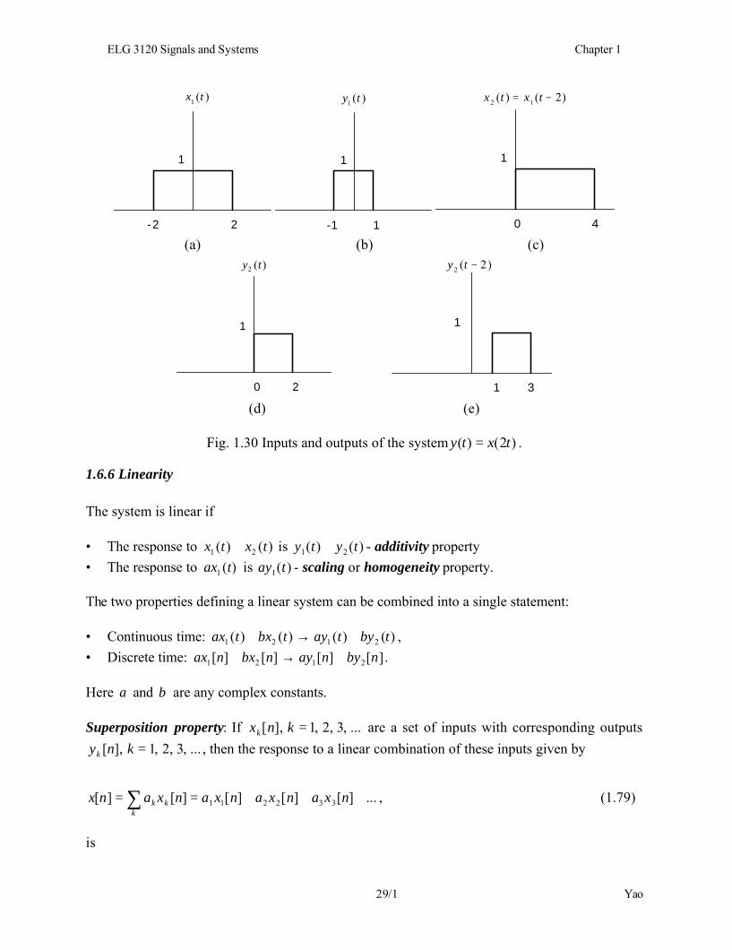
• The system )2()( txty = is not time invariant. To check using counterexample. Consider

)(1 tx shown in Fig. 1.30 (a), the resulting output )(1 ty is depicted in Fig. 1.30 (b). If the input is shifted by 2, that is, consider )2()( 12 −= txtx , as shown in Fig. 1.30 (c), we obtain the resulting output )2()( 22 txty = shown in Fig. 1.30 (d). It is clearly seen that

)2()( 12 −≠ tyty , so the system is not time invariant.


29/1 Yao

-2 2

)(1 tx

1

-1 1

1

)(1 ty

0 4

1

)2()( 12 −= txtx

(a) (b) (c)

0 2

1

)(2 ty

1 3

1

)2(2 −ty

(d) (e)

Fig. 1.30 Inputs and outputs of the system )2()( txty = .

1.6.6 Linearity

The system is linear if • The response to )()( 21 txtx + is )()( 21 tyty + - additivity property • The response to )(1 tax is )(1 tay - scaling or homogeneity property. The two properties defining a linear system can be combined into a single statement: • Continuous time: )()()()( 2121 tbytaytbxtax +→+ , • Discrete time: ][][][][ 2121 nbynaynbxnax +→+ . Here a and b are any complex constants. Superposition property: If ...,3,2,1],[ =knxk are a set of inputs with corresponding outputs

...,3,2,1],[ =knyk , then the response to a linear combination of these inputs given by

...][][][][][ 332211 +++== ∑ nxanxanxanxanxk

kk , (1.79)

is


30/1 Yao

...][][][][][ 332211 +++== ∑ nyanyanyanyanyk

kk , (1.80)

which holds for linear systems in both continuous and discrete time. For a linear system, zero input leads to zero output. Examples: • The system )()( ttxty = is a linear system. • The system )()( 2 txty = is not a liner system. • The system { }][Re][ nxny = , is additive, but does not satisfy the homogeneity, so it is not a

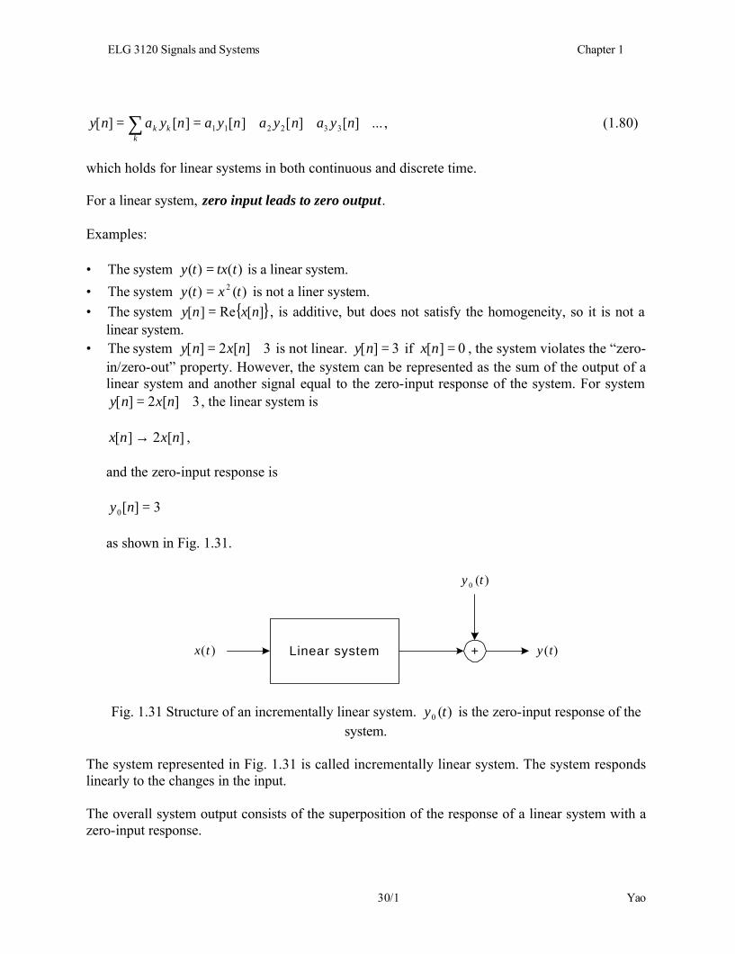
linear system. • The system 3][2][ += nxny is not linear. 3][ =ny if 0][ =nx , the system violates the “zero-

in/zero-out” property. However, the system can be represented as the sum of the output of a linear system and another signal equal to the zero-input response of the system. For system

3][2][ += nxny , the linear system is

][2][ nxnx → ,

and the zero-input response is

3][0 =ny as shown in Fig. 1.31.

Linear system +

)(0 ty

)(ty)(tx

Fig. 1.31 Structure of an incrementally linear system. )(0 ty is the zero-input response of the system.

The system represented in Fig. 1.31 is called incrementally linear system. The system responds linearly to the changes in the input. The overall system output consists of the superposition of the response of a linear system with a zero-input response.

chapter 1 signal and systems

Documents