elec4622: multimedia signal processing chapter 1 ... · elec4622: multimedia signal processing...

ELEC4622:Multimedia Signal Processing

Chapter 1: Continuous and Discrete LSISystems

Dr. D. S. Taubman

July 24, 2007

1 Continuous and Discrete Multi-DimensionalSignals

In this course, we will need to be able to refer both to discretely sampled signalsand continuous signals. In the real-world virtually all signals of interest startout as being continuous. We sample and digitize these signals and perform someprocessing. In order to visualize the processed signals, they must be convertedback into continuous waveforms of one form or another. Not surprisingly then,it is only the underlying continuous representation which can give meaning toour discrete sampled signals and our discrete signal processing algorithms.

1.1 One Dimensional Signals

In one dimension, you should already be familiar with the notion of a continuoussignal f (t) and its discrete sequence of sample values x [n] = f (t)|t=nT . Here,T is the sampling interval and the equation states that x [n] is the sequence ofvalues obtained by evaluating f (t) at the time instants nT where n is an integer.We will find it useful use quite distinct notation for sequences — as in x [n] —and signals or functions — as in f (t). It is worth noting from the outset thatthe sampling interval T is of no fundamental interest. Suppose, for example,that T = 3.912 seconds. In another world, time might be measured in units of(let’s say) zings where one zing in that world is identical to 3.912 seconds inour own. In that world, we would have T = 1 so that all the equations becomemuch simpler.What we are saying is that it is quite sufficient to regard the sampling in-

terval as T = 1 everywhere, no matter what the physical sampling rate mightbe. Then, all that is needed to accommodate reality is to scale our measure-ment units to they physical situation. In the example at hand, with T = 1, the

1

c°Taubman, 2007 ELEC4622: LSI Systems

12−N2n210

column index

row

inde

x

012

1n

11−N

],[ 21 nnx

12−N2n210

column index

row

inde

x

012

1n

11−N

],[ 21 nnx

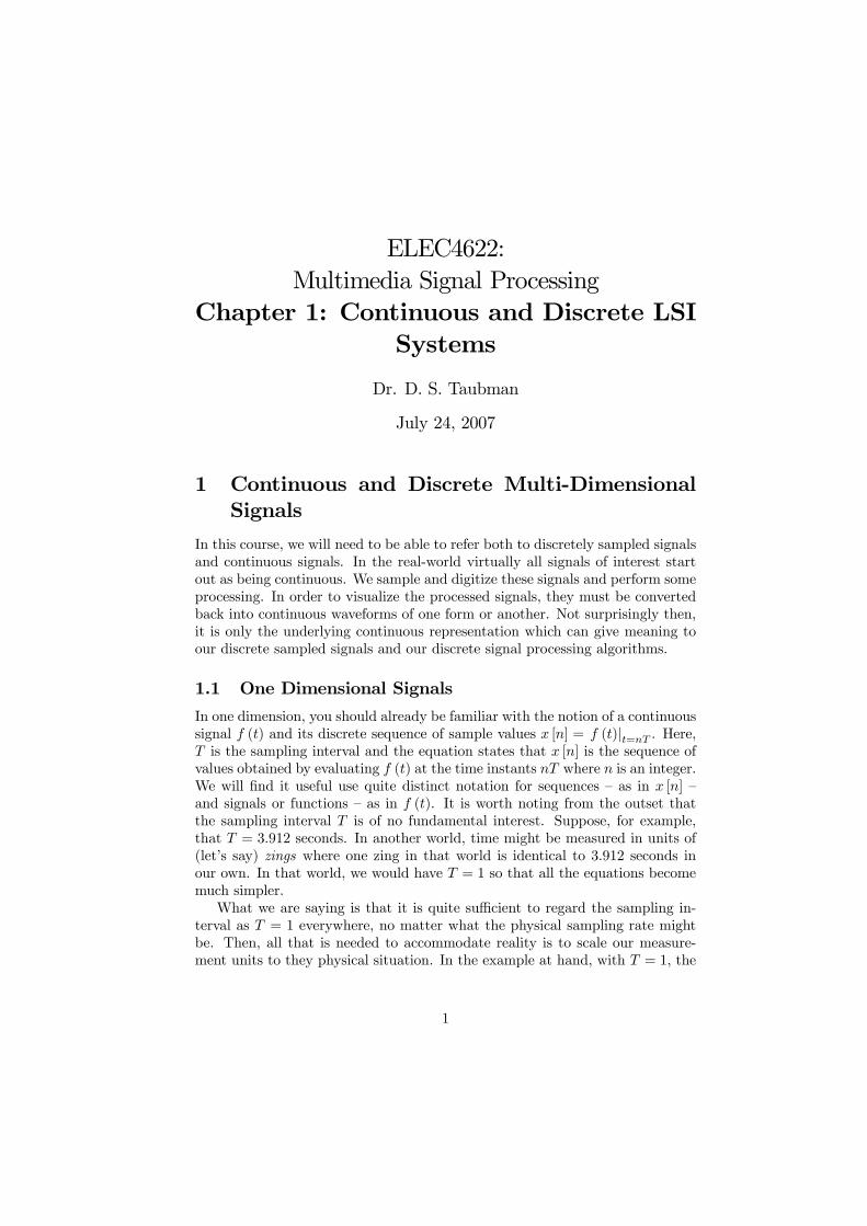
Figure 1: Interpretation of image sample coordinates.

Nyquist frequency becomes fNyquist = 12 , where the units of frequency are cy-

cles/zing. To convert to cycles/s (Hz), we just need to divide by 3.912. Through-out the remainder of this course, all sampling intervals with be 1 and there willbe no reference to specific physical units of time (such as seconds) or distance(such as metres). Frequency is then measured in cycles/unit time. Accordingly,one dimensional sample will always be written as

x [n] = f (t)|t=n

1.2 Two-Dimensional Signals

Discrete images are commonly represented as two-dimensional sequences of pixelvalues,

x [n1, n2] , 0 ≤ n1 < N1, 0 ≤ n2 < N2,

having finite extents, N1 and N2, in the vertical and horizontal directions, re-spectively. The term “pixel,” as used here, is to be understood as synonymouswith an image sample value. The first coordinate, n1 is understood as the rowindex, while the second coordinate, n2, is understood as the column index of thesample or pixel. This is illustrated in Figure 1.The sample value, x [n1, n2], rep-resents the intensity (brightness) of the image at location [n1, n2]. The samplevalues will usually be B-bit unsigned integers. Thus,

x [n1, n2] ∈©0, 1, . . . , 2B − 1ª

Most commonly encountered digital images have an unsigned B = 8 bit rep-resentation, although larger bit-depths are frequently encountered in medical,military and scientific applications.


As with one dimensional signals, images are really just samplings of an un-derlying continuous intensity function f (s1, s2), such that

x [n1, n2] = f (s1, s2)|s1=n1,s2=n2We could think of the spatial coordinates (s1, s2) identifying physical locationon a CMOS or CCD sensor array. We could also think of the spatial coordinatesas measuring position on the focal plane of the optical imaging system1. In thesecases, we might consider spatial location to be measured in units of metres, withrespect to some appropriate reference point. However, as mentioned above, itis more convenient to adopt a unit of distance in which the sampling interval isalways 1, as suggested by the equation above.In many cases, the B-bit sample values are best interpreted as uniformly

quantized representations of real-valued intensities, x0 [n1, n2], in the range 0 to1, where 0 represents the darkest pixel intensity and 1 the brightest. Letting h·idenote rounding to the nearest integer, the relationship between the real-valuedand integer sample values may be written as

x [n1, n2] =2Bx0 [n1, n2]

®=2Bf 0 (s1, s2)

®¯s1=n1,s2=n2

(1)

Colour images are typically represented with three values per sample loca-tion, corresponding to red, green and blue primary colour components. We rep-resent such images with three separate sample sequences, xR [n1, n2], xG [n1, n2]and xB [n1, n2]. More generally, we may have an arbitrary collection of imagecomponents,

xc [n1, n2] , c = 1, 2, . . . , C

Images prepared for colour printing often have four colour components corre-sponding to cyan, magenta, yellow and black dyes; in fact, some colour printersadd green and violet for six primary colour components. Hyperspectral satel-lite images can have hundreds of image components, corresponding to differentbands of the spectrum.

1.3 Three-Dimensional Signals

A discrete three-dimensional signal is a sequence x [n1, n2, n3], indexed by threeintegers. It is often helpful to think of such signals as sequences of images, slicesor frames xk [n1, n2], where the third index n3 = k is the frame number.In a video sequence, the frames xk [n1, n2] correspond to a pictures, usually

captured at a constant frame rate. For example, movies produced for the cinemaare usually played at 24 frames per second. As another example, PAL televisioncontent (Europe and Australia) has a frame rate of 25 frames per second, whileNTSC television sequences (U.S. and Canada) uses a frame rate of 30 frames persecond. Television video sequences have other oddities which we will considerlater in the course.

1These are actually the same interpretation if the scene is in focus.


Another source of three-dimensional signals is volumetric medical imagery.X-ray CT (Computed Tomography), MRI (Magnetic Resonance Imaging) andPET (Positron Emission Tomography) equipment all produce three-dimensionaldiscrete images of the body being imaged. Even though these imaging devicesproduce truly volumetric data, it is common to find that one of the three di-mensions is more coarsely sampled than the other. It is then more natural tothink of the volume as a collection of “slices,” xk [n1, n2], where each slice isa high resolution image and the separation between slices may be larger thanthe separation between the pixels within a slice. Regardless of whether this istrue or not, we can always think of the third index n3 in x [n1, n2, n3] as a sliceindex.In keeping with the conventions developed so far, we shall always regard

discrete 3D signals as the unit-spaced samples of some underlying continuousvolume v (s1, s2, s3), according to

x [n1, n2, n3] = v (s1, s2, s3)|s1=n1,s2=n2,s3=n3

2 Introduction to LSI FiltersFilters play an important role in multimedia signal processing. Filters are de-signed to selectively remove specific features from the image. In this subject, wewill study two types of filters: linear shift invariant (LSI) filters; and non-linearmorphological filters.The features which LSI filters operate on are frequency components — see

Section 3. LSI filters are designed to selectively attenuate specific frequencycomponents. By contrast, non-linear morphological filters can be shown tooperate on the curvature of the edges and intensity surfaces represented bymulti-dimensional signals. Morphological filters are designed to selectively re-move features with excessive curvature. Each type of filter has its own specificapplications.In this section, we briefly introduce the reader to LSI filters and convolution.

These concepts represent an immediate generalization of their counterparts fromone dimensional signal processing. For this reason, we begin by reviewing the1D concepts.

2.1 Discrete-Time LTI Filters

Let x ≡ x[n] be a discrete-time signal (i.e. a sequence, or a function on Z) andH a linear system with H(x) = y. Linearity of H means that if H (x1) = y1and H (x2) = y2, then

H (αx1 + βx2) = αy1 + βy2

for any scalar constants, α and β.It is convenient to write xk ≡ x[n− k] for the signal obtained by delaying x

by k time steps. H is said to be time invariant if for all input signals x,

H(xk) = H(x)k = yk


Hn0

n0

Hn0

n0

k

k

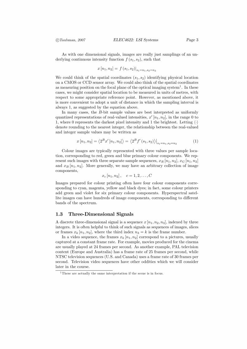
Figure 2: Discrete time invariant operator. Shifting the input signal causes theoutput signal to shift accordingly.

That is, the response of the system to a delayed input signal is a correspondinglydelayed version of the response to the original signal. This is illustrated in Figure2. A linear system which is also time invariant is said to be LTI (Linear andTime Invariant). LTI systems are also called “LTI filters.”Obviously, any sequence x may be written as a linear combination of the

primitive sequences, δi, defined by

δi =

¡ · · · 0 1 0 · · · ¢| {z }i

Specifically, we can always express x as

x =Xi

x[i]δi

Since H is a linear operator we have

y = H(x) = H

ÃXn

x[n]δn

!=Xi

x[i] ·H(δi)

Finally, note that δi ≡ δi[n] = δ[n − i], where δ = δ0 is the unit impulsesequence. That is, δi is a delayed version of the unit impulse sequence. SinceH is time-invariant, we must have H(δi) = H(δ)i and so

y =Xi

x[i] ·H(δ)i =Xi

x[i]hi

where h , H(δ) is the filter’s unit impulse response. Evidently, the LTI filteris entirely characterized by its unit impulse response. Expanding the above


x[n]

0.3

0.7

0.4

n0

0.3δ [n]

0.3

0.7δ [n-1] 0.7

0.4δ [n-2]

0.4

+

+

=

n0

n0

n0

y[n]

n0

0.3h[n]

0.7h[n-1]

0.4h[n-2]

+

+

=

n0

n0

n0

H

H

H

H

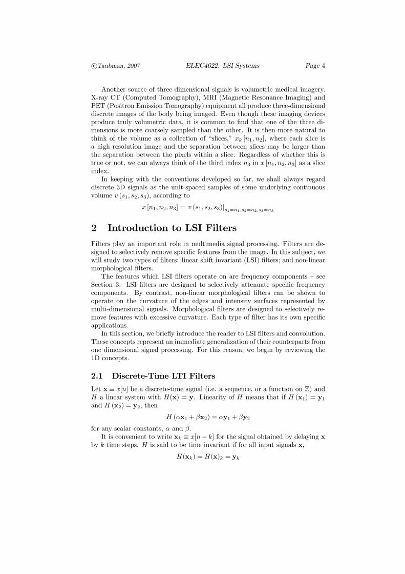
Figure 3: Convolution at work.

expression, we obtain

y[n] =Xi

x[i]h[n− i] =k=n−i

Xk

h[k]x[n− k] = (h x)[n] (2)

which is known as convolution. Figure 3 illustrates the convolution principle.The convolution relationship may alternatively be expressed in terms of inner

products. In particular, we have

y[k] =Xi

x[i]h[k − i] = hx, hki

where h ≡ h[−n] is a time-reversed version of the impulse response, h ≡ h[n],and the inner product (or dot-product) of two sequences is defined by

ha,bi =Xn

a [n] b [n]

Thus, convolution may be implemented by delaying (sliding to the right) h by ktime steps and taking the inner product of this delayed sequence with the inputsequence x, to recover the kth output.


2.2 Extension to Discrete-Space LSI Filters

Let x ≡ x[n1, n2] be a digital image and H a linear system with H(x) = y. Wewill frequently find it convenient to abbreviate the index notation, using the twodimensional vector n, for n1 and n2. Thus, x [n1, n2] may be written as x [n].Write xk ≡ x[n− k] for the image obtained by shifting x down by k1 rows andto the right by k2 columns. H is said to be shift invariant if for all input imagesx,

H(xk) = H(x)k = yk

That is, shifting a filtered image is equivalent to filtering the shifted input image.A linear and shift invariant operator is also called an LSI filter.Following the development of 1D convolution, we find that the output image

produced by the LSI filter can be expressed as

y =Xi

x[i] ·H(δ)i =Xi

x[i]hi (3)

where h , H(δ) is its unit impulse response. In image processing, we use theterm Point Spread Function (PSF), in preference to “impulse response.” An LSIfilter is entirely characterized by its PSF. Expanding equation (3), we obtainthe 2D convolution expression

y[n] =Xi

x[i]h[n− i] =Xk

h[k]x[n− k] = (h x)[n] (4)

Again, the convolution relationship may alternatively be expressed in termsof inner products as

y[k] =Xi

x[i]h[k− i] = hx, hki (5)

where h [n] = h[−n] is formed by reflecting the impulse response through n = 0.Thus, the output of an LSI filter at location k may be obtained by shifting hdown by k1 rows and to the right by k2 columns, and taking the inner product(dot product) of this shifted sequence with the input image x.One important advantage of the adoption of vector notation for our se-

quence and signal coordinates is that the equations that we obtain are true inany number of dimensions. Three dimensional convolution of a video sequence,for example, is characterized by a 3D PSF h [n] ≡ h [n1, n2, n3] and may be im-plemented using either equation (4) or equation (5), noting that all coordinateshave three components and the sums are performed over 3D regions (volumes).

2.3 Spatially Continuous Signals and Filters

Unlike one-dimensional signals, truly continuous processing systems for imagesor video sequences are extremely limited2. Nevertheless, the discrete image and

2That is not to say that continuous multidimensional LSI systems do not exist — opticalsystems, for example, are continuous spatial operators which are approximately LSI. How-ever, we cannot design continuous multidimensional filters using compact analog circuits —something that was readily achievable for one dimensional signals.


video sequences which we do process are most commonly acquired by samplingunderlying spatially continuous scenes. Moreover, digital images and video areoften rendered on a display monitor or printed page, which ultimately producesa spatially continuous representation. For these reasons, we will need to developnotation and an appreciation for spatially continuous LSI operators.Let f ≡ f (s) = f (s1, s2) be a spatially continuous image intensity function

(i.e. a function on R2) and H a linear system with H(f) = g. We writefσ ≡ f(s− σ) for the signal obtained by shifting f down by an σ1 units and tothe right by σ2 units (also by σ3 time units in the case of video). These shiftsare arbitrary real numbers. H is shift invariant if for all input signals f , we have

H(fσ) = H(f)σ = gσ

That is, the response of the system to a shifted input image is a correspondinglyshifted version of the response to the original image. Linear Shift Invariant (LSI)operators are also called filters.Following the discrete development, we can write (in two dimensions)

f(s) =

Z Zf(σ) · δ(s− σ) · dσ1dσ2 (6)

where δ(s) is the Dirac delta function. This is not a real function, but a distri-bution — it “measures” a function at some point. The Dirac delta function isdefined, in fact, by equation (6). We think of δ ≡ δ(s) as the unit impulse image(or video), even though it is not a physically realizable signal. Its integral (2Dintegral over s1 and s2 or 3D integral over s1, s2 and s3) is equal to 1, but itsmass is all concentrated at s = 0. By analogy with the discrete case, we have

g = H(f) =

Zf(σ) · hσ · dσ

where h = H(δ) is the response of the LTI system to the unit impulse and thevector dσ reminds us that this is an integral over multiple dimensions. Theanalogy may be made rigorous, but we do not attempt to do so here. In imageprocessing, h ≡ h (s1, s2) is known as the spatially point spread function (PSF)of the spatially continuous LSI operator, H. Writing the above equation in fullwe have

g(s) =

Zf(σ) · hσ(s) · dσ

=

Zf(σ) · h(s− σ) · dσ

=

Zh(κ) · f(s− κ) · dκ

= (h f)(s)

which is the familiar convolution integral in multiple dimensions.


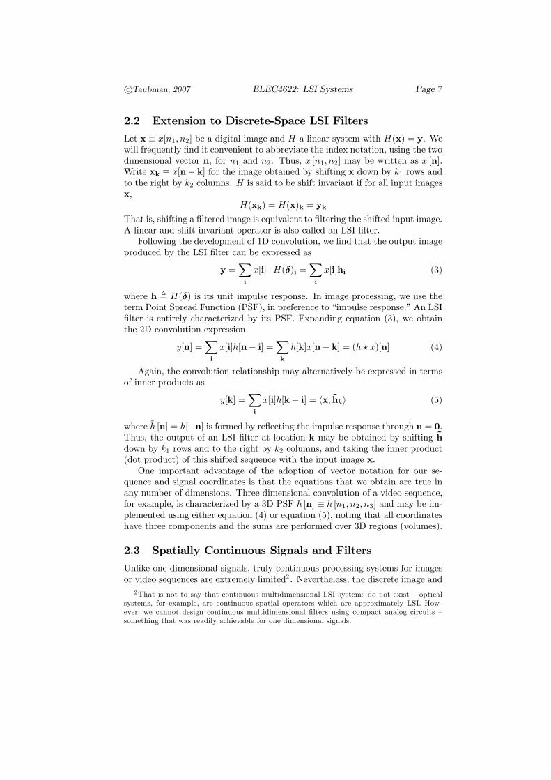
Figure 4: Three sinusoidal intensity patterns.

3 Frequency in Multiple DimensionsConsider the spatially continuous image whose intensity satisfies

f (s1, s2) = A cos (ω1s1 + ω2s2 + φ) (7)

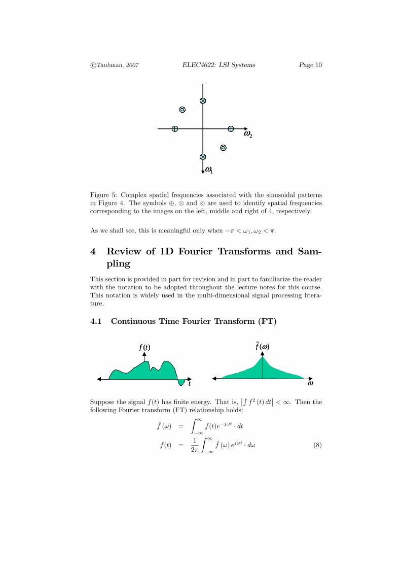
This intensity pattern has only one spatial frequency, with vertical and hor-izontal components, ω1 and ω2, respectively. To help you appreciate spatialfrequency, Figure 4 shows three different sinusoidal intensity patterns. The firsthas ω1 = 0 so there is sinusoidal variation only in the horizontal direction. Inthis case, each row of the image has the same 1D sinusoidal waveform. Thesecond has ω2 = 0 so that each column of the image has the same 1D sinusoidalwaveform. The third image in Figure 4 has ω1 = ω2. Evidently, this results ina rotated version of the sinusoidal patterns seen in the other images. Indeed, itis not hard to show that rotating the sinusoidal frequency vector, ω = (ω1, ω2)

t

through an angle θ rotates the spatial intensity pattern through the same angle,θ.As in 1D signal processing, we will find it convenient to work with complex

spatial frequencies of the form

Aejωts+φ = Aej(ω1s1+ω2s2+φ) = A cos (ω1s1 + ω2s2 + φ)+jA sin (ω1s1 + ω2s2 + φ)

Evidently, the real-valued spatial sinusoid in equation (7) is the sum of twocomplex-valued sinusoids

f (s1, s2) =1

2Aejω

ts+φ +1

2Ae−jω

ts−φ

These two complex-valued sinusoids have frequencies ω and −ω, with phases φand −φ, respectively. The spatial frequencies corresponding to the examples inFigure 4 are depicted in Figure 5. This figure reinforces the fact that rotatingthe spatial frequencies through an angle θ is equivalent to rotating the imagethrough the same angle θ.For discrete digital images, exactly the same considerations apply, with

x [n1, n2] = A cos (ω1n1 + ω2n2 + φ) =1

2Aejω

tn+φ +1

2Ae−jω

tn−φ


1ω

2ω

1ω

2ω

Figure 5: Complex spatial frequencies associated with the sinusoidal patternsin Figure 4. The symbols ⊕, ⊗ and } are used to identify spatial frequenciescorresponding to the images on the left, middle and right of 4, respectively.

As we shall see, this is meaningful only when −π < ω1, ω2 < π.

4 Review of 1D Fourier Transforms and Sam-pling

This section is provided in part for revision and in part to familiarize the readerwith the notation to be adopted throughout the lecture notes for this course.This notation is widely used in the multi-dimensional signal processing litera-ture.

4.1 Continuous Time Fourier Transform (FT)

)(tf

t

)(ˆ ωf

ω

)(tf

t

)(ˆ ωf

ω

Suppose the signal f(t) has finite energy. That is,¯R

f2 (t) dt¯< ∞. Then the

following Fourier transform (FT) relationship holds:

f (ω) =

Z ∞−∞

f(t)e−jωt · dt

f(t) =1

2π

Z ∞−∞

f (ω) ejωt · dω (8)


4.2 Some Properties of the Fourier Transform

Conjugate Symmetry: If f(t) is a real-valued function,

f(ω) = f∗(−ω),where a∗ denotes the complex conjugate of a.

Time shift: Let fτ (t) = f(t− τ), i.e. fτ (t) is obtained by delaying the signalf(t) by time t; then

fτ (ω) = e−jωτ f(ω).

Convolution: Let g(t) = (h f)(t) be the convolution of signal f(t) and theimpulse response, f(t), of an LTI filter; then

g(ω) = h(ω)f(ω).

We say that h(ω) is the transfer function of the LTI system.

Parseval’s relation: Z ∞−∞

|f(t)|2 · dt = 1

2π

Z ∞−∞

¯f(ω)

¯2· dω

4.3 Some Important Examples

Impulse: f(t) = δ(t) =⇒ f(ω) = 1,∀ω. Similarly, f(t) = 1,∀t =⇒ f(ω) =δ(ω).

Rectangular pulse (time domain): Define the “pulse” function,

Π(t) =

½1 if |t| < 1

20 if |t| ≥ 1

2

Its Fourier transform, Π(ω), is given by

Π(ω) = sinc(ω

2π) =

sinω/2

ω/2

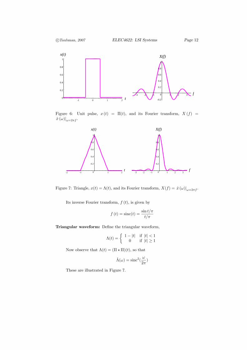
These are illustrated in Figure 6.The way to remember this is that thenulls of the Fourier transform of a unit length pulse lie at multiples ofω = 2π. This is because these frequencies correspond to sinusoids whichexecute a whole number of cycles within the unit duration of the pulse,and hence integrate out.

Rectangular pulse (Fourier domain): Let f (ω) be the unit pulse on theinterval, ω ∈ (−π, π),

f(ω) =

½1 if |ω| < −π0 if |ω| ≥ π


0

0.2

0.4

0.6

0.8

1

-1 0 1 2 t

x(t)

-0.2

0

0.2

0.4

0.6

0.8

1

-3 -2 -1 1 2 3 f

X(f)

Figure 6: Unit pulse, x (t) = Π(t), and its Fourier transform, X (f) =x (ω)|ω=2πf .

0

0.2

0.4

0.6

0.8

1

-2 -1 1 2 0

0.2

0.4

0.6

0.8

1

-3 -2 -1 1 2 3t f

x(t) X(f)

Figure 7: Triangle, x(t) = Λ(t), and its Fourier transform, X(f) = x (ω)|ω=2πf .

Its inverse Fourier transform, f (t), is given by

f (t) = sinc(t) =sin t/π

t/π

Triangular waveform: Define the triangular waveform,

Λ(t) =

½1− |t| if |t| < 10 if |t| ≥ 1

Now observe that Λ(t) = (Π Π)(t), so that

Λ(ω) = sinc2(ω

2π)

These are illustrated in Figure 7.


4.4 Discrete Time Fourier Transform (DTFT)

Let x[n] be any sequence with finite energy. That is,¯P

n x2 [n]

¯< ∞. The

following Discrete Time Fourier Transform (DTFT) relationship holds,

x(ω) =∞X

n=−∞x[n]e−jωn

x[n] =1

2π

Z π

−πx(ω)ejωn · dω (9)

Note that we define x (ω) only on the interval (−π, π). In fact, given any finiteenergy function, x (ω), defined on (−π, π), there is a corresponding sequencex [n], which satisfies the above equations.It is not difficult to show that convolution in the discrete time domain corre-

sponds to multiplication in the frequency domain, exactly as in the continuoustime domain. Specifically, if y [n] = (x h) [n], then y (ω) = x (ω) h (ω).

4.5 Connection between FT, DTFT and Sampling

The relationship between the FT and DTFT is particularly important, sincewe often need to deal with both discrete-time and continuous signals together.This relationship is embodied by the sampling theorem, which we develop inthe following simple steps:

• Let f(t) be a continuous signal with Fourier transform, f(ω).• Let x[n] be the sequence obtained by impulsively sampling f(t) with aunit sampling interval, i.e.

x[n] = f(t)|t=n (10)

and let x(ω) denote the DTFT of x[n].

• Suppose that f(t) is a bandlimited signal withf(ω) = 0, |ω| ≥ π (11)

• Observe that in this case the inverse DTFT integral and the inverse FTintegral, given in equations (9) and (8) respectively, are identical. Specif-ically, we see that

1

2π

Z π

−πx(ω)ejnω · dω = x[n] = f(t)|t=n =

1

2π

Z π

−πf(ω)ejnω · dω

so that f(ω) and x(ω) must be identical. Since knowledge of x(ω) isequivalent to knowledge of x[n] and knowledge of f(ω) is equivalent toknowledge of f(t), we conclude that the sampled sequence x[n], capturesall the information in the continuous signal f(t), provided equation (11)is satisfied. This is commonly known as Nyquist’s sampling theorem.


FT

DTFTsa

mple

identi

fy

inter

polat

e

)(tf )(ˆ ωf

)(ˆ ωx][nx

FT

DTFTsa

mple

identi

fy

inter

polat

e

)(tf )(ˆ ωf

)(ˆ ωx][nx

Figure 8: Interpolation of a bandlimited continuous signal, f(t), from its impulsesamples, x[n], based on the DTFT and FT relationships.

• To reinforce the above observation, we show how the original continuoussignal, f(t), may be recovered from x[n]. The above reasoning is compactlyrepresented by the commutative diagram in Figure 8.Since we are able toidentify f(ω) with x(ω), it must be possible to reconstruct f(t) by firstapplying the forward DTFT to x[n] and then applying the inverse FT tothe result. We obtain

f(t) =1

2π

Z π

−πf(ω)ejωt · dω

=1

2π

Z π

−πx(ω)ejωt · dω

=1

2π

Z π

−π

Ã ∞Xn=−∞

x[n]e−jωn!ejωt · dω

=∞X

n=−∞x[n]

1

2π

Z π

−πejω(t−n) · dω

=∞X

n=−∞x[n] sinc (t− n) =

∞Xn=−∞

x[n] sincn (t)

Thus, f(t) may be obtained directly from x[n], by so-called sinc inter-polation. Specifically, we interpolate the samples by translating a sincfunction to each sample location, weighting the translated sinc functionby the relevant sample value, and summing the weighted, translated sincfunctions.

• The interpolation formula above provides a basis for the space of signalsbandlimited to ω ∈ (−π, π). Specifically, any signal, f ≡ f(t), in this


)(ˆ ωf

ω

ω

)(ˆ ωx

π3− π− π+ π3+

)(ˆ ωf

ω

ω

)(ˆ ωx

π3− π− π+ π3+

Figure 9: Aliasing contributions to the DTFT, x (ω), of a sequence sampledbelow the Nyquist rate.

space, may be represented as a linear combination of the signals, ψn ≡sinc (t− n), with

f =∞X

n=−∞x[n]ψn

In fact, it is not difficult to show that {ψn} is an orthonormal basis, sothe sampling relationship is an orthonormal expansion of f(t) and we haveanother Parseval relationship:

∞Xn=−∞

|x[n]|2 =Z ∞−∞

|f(t)|2 · dt

• As a final note, we point out that signals are not generally exactly ban-dlimited to any frequency range. For non-bandlimited signals, the equalityof f(ω) and x(ω) no longer holds and we find that

x(ω) =∞X

k=−∞f (ω − 2πk)

Thus, the spectrum of the discrete sequence is generally a sum of “aliasing”components, as shown in Figure 9.

5 Multi-Dimensional Fourier Transforms andSampling

5.1 Sampling and Interpolation in Two Dimensions

The Fourier transform and sampling relationships derived above extend directlyto multiple dimensions and, in particular, to images and video.


The 2D FT of a spatially continuous image f (s) = f (s1, s2) is writtenf (ω) = f (ω1, ω2) and satisfies the following relationships:

f (ω) =

Z Zf(s)e−jω

ts · ds1ds2

f(s) =1

(2π)2

Z Zf (ω) ejω

ts · dω1dω2 (12)

The 2D DSFT (Discrete Space Fourier Transform) of a discrete digital imagex [n] = x [n1, n2] is written x (ω) = x (ω1, ω2) which we deliberately define onlywithin the region ω ∈ [−π, π]2 — i.e., −π ≤ ω1, ω2 ≤ π. We refer to this as theNyquist region. The 2D DSFT relationships are:

x(ω) =Xn

x[n]e−jωtn

x[n] =1

(2π)2

Z π

−π

Z π

−πx(ω)ejω

tn · dω1dω2 (13)

Identifying the right hand sides of equations (12) and (13), exactly as inthe 1D case, we find that the discrete and continuous Fourier transforms areconnected through a Nyquist cycle exactly like that shown in Figure 8. Thismeans that so long as a continuous image f (s) is bandlimited to the Nyquistregion, ω ∈ [−π, π]2, its unit sample sequence x [n] = f (s)|s=n is a discretedigital image whose DSFT is identical to the FT of the original continuousimage. Consequently, the interpretation of the spatial frequency components inx (ω) and f (ω) is the same.From a different perspective, the Nyquist cycle implies that for each digital

image x [n], there is a corresponding bandlimited spatially continuous imagef (s), such that x (ω) = f (ω) and x [n] = f (s)|s=n. This spatially continuousimage may be recovered by sinc interpolation, as follows:

f (s) =Xn

x [n] g (s− n) where g (s) = sinc (s1) sinc (s2)

The effect of LSI filtering is convolution by the PSF in the space domainand multiplication by its Fourier transform in the frequency domain. This istrue for both the DSFT and the FT. Combining this with the sampling resultabove, we may draw the following important conclusion. Suppose the digitalimage x [n] is convolved by the discrete impulse response h [n], producing thefiltered digital image, y [n] = (x h) [n]. Then there exist Nyquist bandlimitedspatially continuous images, f (s) and g (s), such that

x [n] = f (s)|s=n , y [n] = g (s)|s=nx (ω) = f (ω) , y (ω) = g (ω)

y (ω) = x (ω) h (ω) g (ω) = f (ω) h (ω)y [n] = (x h) [n] g (s) = (f h) (s)


where h (s) is a Nyquist bandlimited spatially continuous PSF obtained by sincinterpolation of the original discrete digital PSF h [n]. Thus, whenever we arefiltering a digital image, we are effectively filtering an underlying spatially con-tinuous image.The fact that convolution in the space domain is equivalent to multiplica-

tion in the Fourier domain means that the image features which are actually“filtered” by LSI operators are the spatial frequency components. This is be-cause each LSI filter selectively attenuates (or possibly amplifies) each spatialfrequency component, x (ω), of its input image, x [n].

5.2 Some Additional Properties of the 2D Fourier Trans-form

Conjugate Symmetry: If x [n] (resp. f (s)) is real-valued, its Fourier trans-form exhibits conjugate mirror symmetry through the origin of the 2Dfrequency plane:

x(ω) = x∗(−ω) (resp. f(ω) = f∗(−ω))

Spatial shifts: Let fσ(s) = f(s − σ), i.e. fσ(s) is obtained by shifting f (s)down by σ1 units and to the right by σ2 units; then

fσ(ω) = e−jωtσ f(ω)

This relationship is that of a filter with unit magnitude response and aphase response which is a linear function of ω (linear phase filter). Itfollows that whenever a digital image is filtered using a unit magnitudelinear phase filter, h [n], having transfer function h (ω) = e−jω

tσ, theunderlying spatially continuous image is effectively shifted by the vectorσ, regardless of whether or not σ1 and σ2 correspond to whole pixel shifts.

Parseval’s relation:Z Z|f(s)|2 · ds1ds2 =

1

(2π)2

Z Z ¯f(ω)

¯2· dω1dω2X

n

|x [n]|2 =1

(2π)2

Z π

−π

Z π

−π|x(ω)|2 · dω1dω2

Moreover, where f (s) and x [n] are related through the Nyquist cycle (i.e.,f (s) is Nyquist bandlimited and x [n] = f (s)|s=n),X

n

|x [n]|2 =Z Z

|f(s)|2 · ds1ds2

Rotation: One important property of the continuous Fourier transform whichhas no analog in one dimension is that it commutes with rotation. That is,


if fθ (s) is obtained by rotation f (s) through an angle θ then the Fouriertransform of the rotated image fθ (ω) may also be obtained by rotatingf (ω) through the same angle. This fact has already been foreshadowedin the discussion of two-dimensional frequency in Section 3; it is worthgiving a brief proof here. Let

Rθ =

µcos θ sin θ− sin θ cos θ

¶be the matrix operator which effects clockwise rotation of a column vectors about the origin, through an angle θ. You should verify on paper thatthis is indeed the case, noting our convention that s1 is positive in thedownward direction and s2 is positive in the rightward direction. Nowwhen we rotate an image clockwise by θ, each point s in the rotated imageis actually derived from a point in the original image at location R−θ · s —again, you should convince yourself of this with a piece of paper. That is,

fθ (s) = f (R−θ · s)

It follows that

fθ (ω) =

Zf (R−θ · s) e−jωts · ds

=

Zf (κ) · e−jωtRθκ · d (Rθκ) [substituted κ = R−θs]

= det (Rθ)

Zf (κ) e−j(R

tθω)

tκ · dκ

= det (Rθ)

Zf (κ) e−j(R−θω)

tκ · dκ [used Rtθ = R−θ]

= f (R−θ · ω) [used det (Rθ) = 1]

It is worth noting that rotation of a discrete image sequence by anythingother than a multiple of 90◦ does not have an obvious meaning or imple-mentation all by itself. However, an appropriate meaning can be inferredthrough the continuous case. See if you can use the Nyquist cycle to de-duce a sequence of operations which would produce a meaningful rotationoperator for discrete images.

5.3 Extension to Three Dimensions

In the foregoing treatment, there is nothing that we have done which can-not be trivially extended to any number of dimensions. For each discrete3D sequence x [n] ≡ x [n1, n2, n3], there is a unique bandlimited 3D functionf (s) ≡ f (s1, s2, s3) such that

x [n] = f (s)|s=n


andf (ω) 6= 0 =⇒ ω ∈ [−π, π]3

Within the Nyquist frequency cube [−π, π]3, the true Fourier transform of thecontinuous function f (s) is identical to the DSFT x (ω) of the discrete functionx [n], so that discrete LSI filtering on x [n] is precisely equivalent to continuousLSI filtering on f (s). If we need to recover f (s) from x [n], we can (at least inprinciple) use sinc interpolation:

f (s) =Xn

x [n] g (s− n) where g (s) = sinc (s1) sinc (s2) sinc (s3)

As in the case of two dimensions, three dimensional Fourier Transformsexhibit conjugate symmetry through the origin. Moreover, taking the Fouriertransform of the continuous signal f (s) after rotation is equivalent to rotatingthe Fourier transform f (ω). This fact provides fundamental meaning to discretevolumetric rotation operators.One operation which is very closely related to rotation in a video sequence is

motion. Let f (s, t) ≡ f (s1, s2, t) denote a spatio-temporally continuous videoscene, where we have explicitly identified time t as the third ordinate. Nowsuppose we create a new video scene fv (s, t) by subjecting f (s, t) to a globalmotion with velocity v ≡ (v1, v2). That is,

fv (s, t) = f (s− v · t, t)

We can write this asfv (s) = f (R−v · s)

where

s =

⎛⎝ s1s2t

⎞⎠and

Rv =

⎛⎝ 1 0 v10 1 v20 0 1

⎞⎠The coordinate transformation matrix Rv is similar to a rotation matrix. Rvis a “skew” matrix; it causes successive time slices to be progressively shiftedin the direction of v, which skews the spatio-temporal volume. Like rotation,det (Rv) = 1. Also, like rotation, the inverse of Rv is trivially given by R−1v =R−v. Rotation matrices can in fact be constructed from a concatenation ofcarefully designed skew matrices, although that does not specifically matter tous here.


Using Rv we can follow exactly the same derivation provided in the previoussub-section for the case of rotation in two dimensions. We obtain:

fv (ω) =

Zf (R−v · s) e−jωts · ds

=

Zf (κ) · e−jωtRvκ · d (Rvκ) [substituted κ = R−vs]

= det (Rv)

Zf (κ) e−j(R

tvω)

tκ · dκ

= f¡Rtv · ω

¢[used det (Rv) = 1]

We see that the application of motion transforms the Fourier spectrum in ac-cordance with Rt

v. Unlike motion, Rtv is not the same as R−v so the skewing

operation in space-time is a different skewing operation in the Fourier domain.To be precise, we have

Rtv · ω =

⎛⎝ 1 00 1v1 v2 1

⎞⎠⎛⎝ ω1ω2ωt

⎞⎠ =

⎛⎝ ω1ω2

ωt + v1ω1 + v2ω2

⎞⎠That is, the Fourier coefficient at location (ω, ωt) in f gets shifted to the newlocation (ω, ωt − ωtv) in fv. What this means is that the spatial frequencyplane at any given temporal frequency ωt gets skewed (or “tilted”) in the man-ner depicted in Figure 10. Using this interpretation, you can figure out whatthe spectrum of a moving object should look like, by first considering the 3Dspectrum of the stationary object.As with rotation, it is not immediately obvious what a motion transforma-

tion would mean or how it would be implemented in the case of discrete videosequences. However, we can always deduce an appropriate meaning by invokingthe Nyquist cycle. This is the subject of an important tutorial problem.


1ω

2ω

tω

1

1v−

1

2v−

1ω

2ω

tω

1

1v−

1

2v−

Figure 10: Impact of motion v on the location of a plane in the 3D spectrum ofa video scene.

elec4622: multimedia signal processing chapter 1 ... · elec4622: multimedia signal processing...

Documents