Chapter 1: Introduction

1.1 Purpose of the study

The purpose of the study is to understand advertising effectiveness in NGO-

Corporate partnerships. The results will assist both corporates and NGOs in

designing effective advertising campaigns when addressing social issues.

Understanding the factors will ensure that the advertisements used in social

marketing will be effective and relevant to the target market.

1.2 Context of the study

Advertising plays an important role in changing the perception, behaviours and

consumption patterns of society. Society needs advertisements for numerous

reasons including consumer or audience persuasion, information sharing and

decision-making, to name just a few (Indu & Jagathy Raj, 2012)

A number of factors have been identified by numerous researchers as elements

that influence the audience attitude towards advertising such as source

characteristics, target market characteristics, cultural aspects, content used,

media characteristics, credibility, creativity and cognitive routes processing

(Abdulmajid, 2009). These factors would influence the effectiveness of an

advertisement. (Indu & Jagathy Raj, 2012)

Advertising has played a vital role in addressing social issues, such as reduction

of drunken driving, reduction of HIV/AIDS infections, anti-smoking campaigns. A

key social issue on South African roads is drunk driving or driving under the

influence of alcohol. This can be defined as driving with a certain amount of

alcohol in an individual’s blood. Urine tests, blood tests and breathalyser tests

are tools used to determine the amount of blood alcohol concentration (BAC). It

is important to note that 65% of deaths and injuries on South African roads are

due to alcohol abuse (SADD, 2013). Corporates, government and non-

governmental organisations attempt to sell the idea of change to target

audiences regarding drunk driving.

2

In South Africa, The Department of Transport in KwaZulu-Natal launched the

Asiphephe (isiZulu word for Let us be safe) and Siyabakhumbula (isiZulu for We

remember them) campaigns that were aimed at educating the public on drunk

driving through emotional appeal (National Road Safety Strategy, 2011).

Launched in 1998, the Siyabakhumbula campaign would put a human face to

those who would be traumatised directly by drunk drivers. This would include the

paramedics (and other emergency service employees) and the families of those

who died. Through the use of advertising in different media (TV, print) the

campaign emphasised that those in mourning were not in isolation and

highlighted the impact that road accidents have on emergency workers and

victims’ families. The Siyabakhumela campaign was finally ended at an event

held in the province with an attendance of over 40 000 people affected by drunk

driving and those wanting to publicly display support of anti-drinking and driving

behaviour.

In partnership with business and non-governmental organisations, the Asiphephe

campaign focused on those persons and families left to deal with the severely

injured or disabled persons. The advertising campaign also emphasised the lack

of support given to the less privileged and the disabled. Well-known personalities

(sportsmen, actors, and musicians), civil leaders and religious leaders were also

used to endorse the campaign, explaining how drunk drivers had affected them

in the different advertisements of the campaign. Aimed at the KwaZulu- Natal

youth that are mostly responsible for the pandemics in the province, the

campaign used music to further expand on the emotional appeal. A road safety

CD was launched through partnerships with famous international and national

musicians. Though the campaigns received criticism, KwaZulu-Natal was the

only province that reduced road deaths by 35% compared to the average of 17%

in the rest of South Africa (National Road Safety Strategy, 2011)

In 2009 through a partnership between an NGO, corporate and public sector, the

“name and shame” campaign against convicted drunk drivers in the Western

3

Cape was launched. The aim of the campaign was to discourage drunk driving

behaviour through public humiliation. The campaign has been pivotal in reducing

road fatalities by 30% (Times Lives, 2009). Through the use of local media, the

Cape Argus would publish the names of those people who had been convicted of

drunk driving. Arrest patterns changed drastically in the weeks in which the list

appeared. The use of radio (Talk Radio 702 FM and Lead SA) and print

newspapers were used to advertise the campaign (Williams, 2013).

The above campaigns also made use of partnership across the three sectors.

Strategic partnerships are beneficial for all the sectors (public, private and non-

profit organisations). Reputation improvement (Falck & Heblich, 2007), sympathy

towards stakeholders concerns and relations (Smith, 1994; Webb & Mohr, 1998

as cited by Hall,Jones & Iversen, 2011), volunteerism and product innovations

are motivations for companies to partner with NGOs. For the NGO, it is an

opportunity to improve awareness, allows for networking opportunities, resource

support and to increase their influence. (Runte, 2009, as cited by Simpson,

Lefroy & Tsarenko, 2011; Polonsky, Wood, Varadarajan & Menon, 1988, as cited

in Hall et al.,, 2011)

The use of partnerships between NGOs and corporates has increased in South

Africa in the past decade. Companies with a turnover of over R5 million are

required by the Broad Based Black Economic Empowerment Act 53 of 2003 to

invest 1% of net profits into socio-economic development, hence the growth in

the partnership. Kourula (2006) identifies the following as partnership options that

companies and NGOs could engage:

I. Sponsorship: the NGO receives financial support from the company which

could include marketing cooperation;

II. Single-issue consultation: The company consults an NGO on a social or

environmental issue. This could include advice on a particular company

product;

4

III. Research cooperation: The NGO and company provide resources for a

research project of interest to either/both parties;

IV. Employee training or volunteerism: NGO employees are requested to

address employees on a particular issue that the NGO would work with or

employees from the company are volunteering to assist at the NGO;

V. Certification or eco-labelling: An NGO certifies a company product or

service as having met environmental or social standards;

VI. Systematic Dialogue: The company and NGO have systematic discussion

or forums to discuss vital issues;

VII. Common projects/programmes: NGO and company collaborate in a single

project with defined actions and clear objects; This research paper aims to

understand the impact of this partnership on social marketing advertising.

VIII. Strategic partnerships: NGO and company sign a long-term partnering

agreement with long-term goals, for example the Coca-Cola Company and

USAID) (Kourula & Halme, 2008).

The process of identifying a suitable partner is important because of the need to

recognise similar objectives, ensure access to target audience, credibility within

the targeted audience, interest in the initiative and resources needs (Acsinia,

2010).

Consequently, this study will also attempt to understand perceptions and attitude

towards the co-sponsoring advertising in comparison to a specific advertisement,

either corporate or NGO-sponsored.

1.3 Research problem

A social marketing advertisement campaign may not attain expected results for

many reasons; audience resistance can arise at any stage between exposure

and behaviour implementation (Rice & Atkins, 2013)

In social marketing advertisement design, the common mistake is assuming that

portraying behaviour as unhealthy or bad will cause people (especially children)

5

to reject it. In fact, the display of behaviour as prohibited may enhance the appeal

to adolescents. It is also suggested that consistency in messaging from other

sources generally affects the success of public communication campaigns.

Public communication campaigns must provide a consistent messaging from

various sources over a long period to be effective and have credibility (Austin,

1995 as cited in Siegel, 1998). The credibility of an advertisement refers to a

person’s perception of the truth presented in the content. It can be discussed in

other forms, including corporate credibility (the perceived truthfulness of the

perceived sponsor) and ad credibility (message content and endorsers’ credibility

(MacKenzie & Lutz, 1989 as cited by Indu & Jagathy Raj, 2012)

In some countries, alcohol producers will sponsor NGOs who aim to address

alcohol-related issues. This would include campaigns against drunk driving, for

example South African Breweries sponsor some South Africans against Drunk

Driving initiatives.

Research question

The over-arching question guiding this study is: What are the factors affecting

advertising effectiveness in NGO-corporate partnerships when addressing social

issues like drunk driving?

1.4 Research objectives

The research objectives addressed in the study will include:

To conceptualise the factors that affect advertising effectiveness

The integration of the factors that affect advertising effectiveness in

NGO-corporate partnerships with the social issue of drunk driving

To determine the relationship between the factors and attitude towards

advertising effectiveness

To determine if the factors affecting advertising predict the attitude

towards advertising in NGO-corporate partnerships

6

To determine the difference between the factors that affect advertising and

attitude towards NGO-corporate with rigid variables (age, marital status,

education level)

1.5 Significance of the study

Firstly, it will add to academic literature in South Africa by serving as the basis of

understanding the advertising element in NGO corporate partnerships. Future

research would then build on this study, taking into consideration the impact of all

the factors mentioned

Secondly, it explores field of social and NGO marketing that are important in

developing country context because of the social issues in the twenty-first

century. Social issues derive from development, natural resources and

economics dynamics within a country (Tajziehchi, 2011). Social issues in

developing countries include HIV/Aids, malaria, high rates of alcohol

consumption, unclean drinking water, to name a few.

Thirdly, exploring factors that affect advertising effectiveness is important

because it allows social marketers an opportunity to address issues through

advertising in the most impactful way that will lead to behaviour and attitude

change.

Lastly, this will allow the organisations to structure suitable and effective

communication for their social campaigns when pursuing collaboration efforts or

working independently.

1.6 Delimitations of the study

The following are limitation to the study

The study will be conducted in Gauteng through random stratified method

which will to recognise the different gender groups, race and age.

7

Sample is only 300 respondents

The advertising tool used in the study will be print and will exclude other

mediums because of costs pressures and this method has also been

successfully applied in similar studies in developing countries (University

of Wisconsin’s binge-drinking campaign)

The social issue addressed was drunk-driving as this pandemic is on the

rise. Research done by Arrive Alive shows that the likelihood of being in

an accident on a South African road is 1 in 101 but other parts of the world

is 1 in 5000. The Arrive Alive campaign reports that one of the biggest

threats to South African roads is drunk drivers, indicating that 50% of the

deaths on the roads can be directly linked to over-indulgence of alcoholic

beverages and one in fifteen South African drivers on the road at night are

drunk (Arrive Alive, 2012)

The study focused on adults over the legal alcohol-drinking age of 18.

A reputable company and a NGO (which was created for the sake of the

study) will be used to understand the dynamics. South African Breweries

(SAB) was selected because of its efforts in curbing the drunk-driving

pandemic; the alcoholic beverage company currently has just under 90%

market share (Vallie, 2012). SAB is a well-known company in South Africa

and participants will be able to recognise its visual identity. A NGO has

been created for the study because the research failed to produce a

reputable NGO addressing this pandemic. The NGO has been named

People against Drunk Driving (PADD) and a logo was designed for this

made up organisation.

SAB was approached to use the company’s current “Regret nothing”

campaign.

8

Chapter 2: Literature Review

2.1 Introduction

The literature review introduces key concepts for the study. This will include

definitions, backgrounds and theory gathered about the concepts. The literature

review will define and discuss advertising, recognise factors that affect

advertising effectiveness and then select key prominent element to form a

proposed model for this study.

The literature review will also introduce the concept of social marketing that can

be used in advertising.

2.2 Background on Advertising

Advertising is a marketing tool that provides information about a product, service

and the business itself. It has been said that the purpose of advertising is mainly

to build brand image, stimulate purchasing (Park, Shenoy & Salvendy, 2008) and

provide information and appeal (Kumar, 2010 as cited in Dubihlela, 2011). The

American Marketing Association defines advertising as the persuasion of a target

audience or market about products, service or ideas using announcements or

messaging in space or time bought in any mass media. This can be used by

business, nonprofit organisations and government agency (American Marketing

Association, 2013). Advertising plays an important role in changing consumption

pattern and perception of society in general. Society needs advertisement for

various reasons including consumer persuasion, information sharing and

decision making (Indu & Jagathy Raj, 2012). It often incorporates the views of the

majority of the consumers as a persuasive tactic or substantiating

product/service/idea claims (Buchanan and Smithies, 1991 as cited in Chang,

2012).

9

Advertising can be increasingly powerful when it presents products or services

that people do not know they need. It anticipates and exploits the prevailing

consumer attitude and culture. The symbolic relationship between advertising

and the audience ensures that advertising feeds information that shapes the

culture and at other times abstracts elements from popular culture to create the

concepts (Goldberg,2011) Some researchers have accused advertising of selling

dreams and enticing consumers into confusing dreams with reality. Advertisers

cynically use a fantasy world and illusion in an attempt to control the target

audience (Klempner, 2004 as cited by Dubihlela, 2011).

As technology evolves, new types of advertising mediums have been introduced.

First generation advertising mediums included magazines, newspapers and

billboards. Radio and television (TV) were the next generation and are the most

prevalent method of advertising. Recently, mobile and Internet have emerged as

new types of advertising mediums and are rapidly growing (Park, Shenoy &

Salvendy, 2008). Advertising is modifying the manner in which it targets young

people because of young people’s relationship with technology and its devices

(Segovia, 2013).

An effective advert is one that succeeds in anticipating and exploiting the

prevailing consumer culture and attitudes whilst using the correct medium. When

an advert is able to capture the desires or needs, expressed or not, it has a good

chance of succeeding in persuading and selling. The advert must be able to tap

into a meaningful socio-logical, emotional and psychological focal point

(Goldberg, 2011).

The most successful advertisements reflect society and the role that the product,

service or idea can play in the current environment (Goldberg, 2011).

10

In advertising, some advertisements are successful and others fail in achieving

intended objectives. This is affected by the advertisers’ decisions regarding

advertising strategies and tactics (Indu & Jagathy Raj, 2012). A successful advert

according to Kotler, states that information appeal as two parts:

1. Rational appeal: informs audience of the fundamental values of the

product or service. This involves functionality, practicality and quality

2. Emotional appeal: aims to stimulate a purchase based on emotional

response to image and context (Kotler, 1991 as cited as Yeh & Lin, 2010).

2.3 Factors affecting advertisements

The effects of an advertisement are also dependent on several factors and their

contributions vary according to the situation. These factors can be grouped in

three categories, namely advertisement factors, environmental factors and

audience factors.

Figure 1: Effects of advertising as described by Park, Shenoy and Salvendy, 2008

Advertising Effectivess

Advertising factors

Design

content

Envionmental

Factors

Context and distractors

Exposure time and repetition

Audience factors

Experience and attitude

Involvement

11

Advertisement factors include design factors and content. The design of the

advertisement includes size and length of the advert, music/sound effects,

colour, and presence of animation. The design factors relate more to the

transmitting media (multimedia functionality).

The content of an advertisement is the primary factor driving marketers and

advertisers. Content is mainly focused on the presentation of the message and

the story line. It is divided into two groups, namely affective and cognitive. An

informative message depends on the cognitive processing of the audience which

would be effective in relating the functionality of the product whereas the affective

message appeals to the emotional processing (Park, Shenoy and Salvendy,

2008)

Environmental factors include context and distracter, exposure time and

repetition. Context and distracters address the issue of the surrounding of the

audience. Context focuses on the competitive advertisement clutter effect. The

environment where the advert is presented can be a distractor.

Several studies conducted have suggested that the recall rate increases as

exposure time increases. Repetition is also believed to have a positive impact of

the recall rate (Park, Shenoy and Salvendy, 2008).

Audience factors include experience, attitude and involvement. The experience

or exposure to the advertisement tends to build the attitude of the

audience/consumer that can improve or weakened over time. Attitude can be

about the brand, actual advertisement or advertising media. Involvement has

been instrumental in advertising effectiveness studies. It can be defined as

personal connection points between the stimulus and the audience. Involvement

theory suggests that the more the audience is interested in the product, the more

12

they pay attention to the information provided (Park, Shenoy and Salvendy,

2008).

From the literature above, this study proposes the following model (Figure 2) in

understanding factors that affect advertising effectiveness in NGO-corporate

partnerships.

Figure 2: Proposed model for understanding factors affecting NGO-corporate partnerships

2.3.1 Involvement

Involvement is one of the factors used in the study. A study by Wu (2001)

showed a positive relationship between degree of consumer involvement and the

advertising effect hierarchy (6-step hierarchy of effect mode: awareness,

knowledge, liking, preference, conviction and purchase) (Wu, 2001). There is

agreement amongst advertising researchers on the relationship between

involvement and advertising effectiveness (Tipps, Berger, & Weinberg, 2006)

Involvement has been an issue of debate in research. Sherif and Hovland (1961)

have argued that personal involvement occurs when the message has intrinsic

importance or personal meaning (Sherif & Hovland 1961). Involvement has been

hypothesised to lead to greater product importance, greater perception of

attribute differences and greater commitment to the brand choice (Wu, 2001).

According to Zaichkowsky (1994), personal involvement refers to the level of

13

perceived personal relevance or importance evoked by a stimulus within a

certain condition. The person’s perceived relevance is based on inherent values,

needs and interest (Zaichkowsky 1985 as cited in Wang 2009). Zaichkowsky

(1994) suggests that in understanding personal involvements three major

antecedent factors must be studied. Firstly, the character of the person;

secondly, character of the stimulus and finally, the character of the product.

These three factors will influence level of personal involvement in the product,

purchase and advertising (Wu, 2001). Krugman (1965) further elaborates on the

idea by studying this concept from the consumer psychology approach. The

researcher suggests that high involvement will rely on the number of personal

references that the recipients can make between the messages and their own

lives (Krugman 1965 as cited by Petty & Cacioppo 1981).

Wu (2001) recommends a framework of involvement that is affected by personal

and product factors. The base of the framework is formed from work done by

Zaichkowsky (1985) and Andrews (1990). The product factors comprises the

product characteristics. Personal factors are the audience characteristics which

include personal goals, needs, activities, interstices and demographics (Wu,

2001).

Proposition 1:

The relationship between demographics (gender, race, age, educational level,

marital status) and level of involvement

Numerous researchers segment product category by level of audience/consumer

involvement but do not segment the audience by demographics or characteristics

(Wu, 2001)

14

The Elaboration Likelihood Model (ELM) was developed to understand how

recipients process information. ELM suggests that a high level of personal

involvement is the central premise for attitude change (Petty, Cacioppo, &

Schumann, 1983 as cited by Wheeler, 2009). ELM model comprises of two key

elements, central and peripheral route. Central route is when the recipient has an

individual diligence concentration because the information delivered is of

relevance. It is believed that a more permanent or predictive attitude change

would be induced via this route (Cialdini, Levy, Hermann & Kozlowski 1976 as

cited by Petty & Cacioppo 1981). ‘Peripheral route’ refers to when the individual

does not cognitively process the advert but instead associates it to positive or

negative cues (Wang 2009). Attitude changes through this route would make use

of non-content cues like number, quality or accuracy of the presented message

because of lack of interest (Petty & Cacioppo, 1980; Cahiken 1980 as cited in

Petty & Cacioppo, 1981). The change expected is more temporal and non-

predictive.

In the context of social marketing, a cognitive model is regarded as crucial

because of the significance of the message delivered and intractability of the

behaviour belief addressed (Hassan, Walsh, Shiu, Hastings & Harris, 2007).

Advertisements in magazines and newspapers are regarded as pull type

because the message is transferred by free will of the audience. This is done to

create high involvement levels of the audience. TV and radio are push type

advertising and the message transferred is controlled by the advertising agency

or marketer. Involvement measurement of the push type advertisement is

relatively low in comparison to advertising on magazines and newspaper

(Krugerman 1967 as cited by Park, Shenoy & Salvendy, 2008). Two mediating

factors, involvement and attitude towards advertising, are broadly studied in

persuasive model framework

15

2.3.2 Source credibility (Trust and Expertise)

Various researchers suggests that use of source with high credibility will increase

reliability (Petty & Cacioppo, 1986; Pornpitakpan 2004 as cited by Hall, Jones &

Iverson 2011) (Helmig & Thaler 2010). The source credibility research can be

traced back to a study done in 1951 by Hovland and Weiss. The study indicated

that recipients attached subjective credibility levels to different sources (Hassan,

Walsh, Shui, Hastings & Harris 2007). Source credibility is the perceived

trustworthiness and expertise of a particular communicator (Wheeler 2009).

Truth is the degree to which the recipient perceives the communicator to convey

valid assertions or degree of confidence in the intent of the communicator. Trust

is towards both communicator and message. Expertise refers to the extent to

which the communicator is deemed knowledgeable and capable of making valid

assertions about the message/object (Howland, Janis & Kelley 1953 as cited by

Wheeler 2009). Source credibility is important to understand and research in

advertising effectiveness because of credible sources and those associated with

extensive levels of expertise are likely to attract high levels of elaborations and

consequently better attitudinal and behavioural changes (Hassan, Walsh, Shui,

Hastings & Harris, 2007). In 1993, Wilson and Shelley found that the greatest

impact of persuasion could be found in using experts and those communicators

who are perceived to have high levels of credibility (Hassan, Walsh, Shui,

Hastings & Harris 2007). Another key element that affects perceived credibility is

presentations. It has also been referred to as attractiveness or image (Ohanion,

1990; Eisend, 2006).

In campaigns addressing social issues, high creditability sources will more likely

change the recipients’ attitude and behaviours (Fragale & Heath, 2004). This was

confirmed by a study done by Mick in 1992 on an anti-smoking campaign. It was

noted that there is an association between levels of credibility and the level of

comprehension in the advertisement. The latter raises questions on whether

advertising is an effective tool for addressing consumer well-being. If the source

16

used is of ‘low-credence’, this is unlikely to affect the behavioural change, leading

to failure in social-NGO marketing goals (Hassan, Walsh, Shui, Hastings & Harris

2007).

Attribution theory aims to explain how recipients develop causal assumptions

regarding motivation of a particular sponsor’s communication of promotional

messages. Szykman, Bloom and Blazing (2004) wrote that depending on

advertising context, it would be advantageous for the message sponsor of a

social marketing advert to be endorsed by a non-commercial source (Szykman,

Bloom & Blazing, 2004).

Proposition 2:

People Against Drunk Driving (PADD) as a sponsor will have high levels of

credibility

Proposition 3:

South African Breweries (SAB)–People Against Drunk Driving (PADD)

partnership sponsors will have a high level of credibility

Research has also revealed that recipients evaluate a company negatively if they

believe its business practices are company-serving as opposed to socially

motivated (Hassan, Walsh, Shui, Hastings & Harris 2007).

Proposition 4:

South Africa Breweries as a sponsor will have low levels of source credibility

When companies address social issues, consumers perceive this as either a

brand image or awareness exercise which decreases the sincerity of the

message (Rieh & Belkin, 1998). The concept of credibility is highly intuitive

17

(Eisend, 2006), so it is important for companies to understand if the recipients

associate the message with them.

The intense competition and great volume of the advertising can confuse the

consumers and create doubts in their minds about the reliability and genuineness

of the advertisement and its products (Indu & Jagathy Raj, 2012). Because

advertising aims to attract interests and tastes of an outsized group of

consumers, it is vital that it provides information about the product or service, as

well as the endorsers (Engel, Blackwell & Miniard as cited in Yen & Lin, 2010).

Credibility is defined as the degree to which the audience perceives claims made

about the product or brand in the advertisement as truthful and believable

(Cottea, Coulterb & Moore, 2005) Advertisements that lack credibility can often

be avoided and ignored by the audience (Rodgers, 2005). Advertising credibility

has been identified as the most important factor in advertising effectiveness.

Credibility is a key factor of persuasive messaging and can often influence the

outcome of a persuasive message (Indu & Jagathy Raj, 2012).

Advert credibility can be classified in two groups: the first is the advertiser’s

credibility (corporate sponsor), and the second, the advertisement credibility

(message content credibility) (Indu & Jagathy Raj, 2012). According to Petty and

Cacioppos (1981), the developers of the Elaboration Likelihood Model (ELM)

discussed above, the advert audience give importance to the advertisement

sponsor and message content when they go through the central route to

persuasion.

Proposition 5:

The relationship between source credibility and level of involvement

18

2.3.3 Message content

Puto and Wells (1984) discuss message content in an advert in two elements:

informational and transformational.

‘Informational advertisement’ was defined as information (about the

brand/product/service) that the advertisement provides to the target audience in

a clear precise and logical manner such that confidence is built in ability to

measure the brand, product or service after viewing the advert. The key element

is that the advert is informational. An advert that is considered informational

contains the following characteristics: (1) it presents factual, important

information about brand; (2) it presents information which is useful and important

to the customer; and (3) the consumer accepts data to be credible and

appropriate. Informative advertising decreases prior inaccuracies that the

consumer may have believed about the product. The customer will absorb all

they need to know about the product and further information will fail at influencing

their decision (Ackerberg, 2003 cited in Martin, 2012). An important element of

the content is the theme used in the communication (Elder, Shults, Sleet,

Nichols, Thompson, & Rajab 2004).

There are three types of informational message in advertisement campaigns: one

creating awareness, the second, instruction messaging, and lastly, persuasive

messaging. In awareness messaging, information presented advises the

audience on what to do, cues on when and where it should be done and

specifies who should do it. The more complex option is the instruction message

which should produce knowledge and skills acquisition, including personal

efficacy enhancement and peer assistance. Persuasive messaging provides

reasons or advocates why the target audience should adopt the presented

prescribed behaviour and avoid certain choices (Rice & Atkins, 2013).

19

A transformational advertisement is one that has the ability to associate the

brand/product/service to a particular psychological characteristic which would not

typically be associated with the brand. A transformational advert would include

the following characteristics: (a) The experience of using the product/service/

programme will be made more fulfilling, thrilling, enjoyable than that expected

from the advert’s objectives; (b) the experience of the advert and the experience

of using the brand/product/service are so closely related that the consumer

cannot recall the brand/product/service without remembering the experience

generated from the advertisement.

In advertising, understanding the audience through research is critical for

developing the initial message. Marketers must be creative around the actual

message and its delivery.

The effectiveness of an advert is dependent on the characteristics of the target

audience and requires a match of the message to the individual motivation or

reason for engaging in the behaviour (Snyder & Cantors, 1998 a cited by

Rhodes, Roskos-Ewoldsen, Eno, & Monahan, 2009)

Proposition 6:

The relationship between the demographics and content

In relation to social marketing, sustained engagement with persuasive and

credible messages addressing belief is important. Advertising themes and

content should be selected for their capability to create favourable cognitive-

based attitudes (Wu, Walsh, Shiu, Hastings and Harris, 2007).

Research done by Tsai & Tsai (2006) suggests that negatively framed

messaging is more effective than positively framed messages in a high-

involvement arena (Tsai & Tsai, 2006 as cited by Pongiannan, 2013). The advert

20

used in the study had a negatively framed message with the theme as “Don’t turn

a good time into doing time”. The play on words is advising the audience not to

drink and drive because they could end up in prison.

Proposition 7:

The negatively framed message content has a high degree of involvement

The “Don’t drink and drive” advertisement mentioned is an example of social

marketing efforts.

2.4 Social Marketing

Public health campaigners have found that the powerful and persuasive mass

media can be used to promote health and other social issues (Siegel, 1998). This

study aims to understand advertising effectiveness when addressing a social

issue (particularly drunk driving). This is known as social marketing which is used

by both business and non-governmental organisations (McKay-Nesbitt &

DeMoranville, 2011). The first definition of social marketing was coined in 1971

by Kotler and Zaltman:

“Social marketing is the design, execution, and control of marketing related

programs that involve the consideration of product planning, price

communication, distribution and market research with the aim to influence the

acceptance of social concepts or ideas within a specific target market” (Kotler &

Zaltman, 1971)

In 1995, Andreasen revised the definition of social marketing as the following;

“Adapting of commercial marketing technologies in the analysis, planning,

implementing and assessment of programs designed to influence the voluntary

bahaviours of a specific target market so as to improve their mental and physical

well-being and/or that of society they are part of” (Andreasen, 1995).

21

Four key features are illustrated in the above definitions. The first is the emphasis

on voluntary behaviour change. Social marketing is not about enforcement or

coercion. The second focus is that social marketers are trying to persuade

change by applying the fundamentals of exchange, recognising that there will be

value and benefits for the target audience if the change occurs. The third feature

is that marketing techniques such as consumer focus, targeting, consumer

research and segmentations, and the marketing mix should be applied. Finally,

social marketing aims to bring about change in the individuals welfare and

society, and not to the benefit of the organisations doing the social marketing

(Stead, Hastings and McDermott, 2007).

In 2007, the American Marketing Association (AMA) extended the definition of

marketing to include the benefits of social marketing:

“Marketing is the approach of generating, communicating, delivering and

exchanging value with marketers, partner organisations, and society as a whole

so as to improve the welfare of individuals and society” (Dann, 2008 as cited by

Alves, 2010).

The definition accepted by the AMA thereby recognises clients as receptors of

social marketing efforts and the co-creation of values amongst the different

stakeholders.

2.4.1 Social marketing versus commercial marketing

Social marketing could counteract the negativities promoted on commercial

marketing (Fox and Kotler, 1980 as cited by O’Shaughnessy, 1996). Where the

primary motivation of marketing is to promote public good – this can be regarded

as social marketing; however, where the primary motivation is to create profit or

any motivation not promoting public good, this is not regarded as social

marketing (Donovan, 2011). Although both social and commercial marketing aim

to change behaviour, social marketing aims to change behaviour that benefits

individuals and society, whilst commercial marketing will benefit the needs of the

22

business and its stakeholders (McKay-Nesbitt and DeMoranville, 2011). One of

the key differences between commercial and social marketing is the fact that

social marketing promotes ideas, products or services for voluntary behaviour to

a specific target market whilst commercial marketing aims to trade a product or

service for economic gains and is not concerned about any healthy behaviour

change amongst the target market (Sharma, 2007). The purpose of a commercial

marketer is self-explanatory: A business will close if people do not purchase its

goods and services (Baker & Saren, 2010).

Table 1 below indicates these differences between social marketing and

commercial marketing.

Table 1: Differences between commercial and social marketing (McKay-Nesbitt and

DeMoranville, 2011)

Commercial Marketing Social Marketing

Creates, communicates and delivers

value in forms of good or services e.g.

beverages, petrol, insurance

Creates, communicates and delivers

value in the form of behaviour, e.g.

reduction of drunk-driving pandemic

or reduction of speed to conserve

petrol

Though commercial marketing can be

concerned about the well-being of

society, its primary concern is

generating financial benefits

Social marketing primary goal is the

betterment of individual and society

Competition in commercial marketing

occurs between providers or suppliers

of similar product offering or service

Competition in social marketing

occurs between existing behaviours

versus new proposed behaviours

In 1952, G.D Wiebe posed a question, “Why couldn’t we sell the concept of

brotherhood like we sold soap?” The question would imply that sellers of

commodities such as soap are generally effective whilst those “selling” social

23

causes were unsuccessful (Kotler and Zaltman, 1971). However, traces of its

application were evident in family-planning awareness campaigns in the 1960s

in the Unites States. In 1969, Kotler and Levy legitimised the academic study of

social marketing by emphasising that the use of marketing needs to be extended

to embrace non-commercial entities (police, non-profit organisations, churches)

(O’Shaughnessy, 1996). In 1971, Kotler and Zaltman defined social marketing-

as noted above. The work by the authors would be critical in the introductory

phase because it defined the term social marketing and initiated the planning

processes (Alves, 2010). The growth of social marketing was further noted when

applied in broader conceptions rather than those of products marketed for social

alteration (condoms, birth control, oral rehydration solution) (Andreasen, 2002).

Consider the following South African pandemics: what do the following issues

have in common: drunk driving, rape, smoking, teenage pregnancy, transmission

of HIV/AIDS and global warming? Firstly, they are pressing issues with great

concern. Secondly, they have a big impact on social welfare and can become a

matter of life and death. The basic trait they share is all have a function of human

behaviour: the perpetrators’ actions and those of people creating social

environment that make them less or more attractive (Baker & Saren, 2010).

Social marketing typically focuses on behaviours that protect one’s health and

safety (such as. smoking cessation, drunk driving), the environment (for example

water conservation) or community well-being (for example. obesity, literacy,

HIV/AID prevention) (McKay-Nesbitt, DeMoranville, 2011).

Social marketing campaigns can be viewed as power strategies to fend off

legislations (for example BAC limit for driving) that could endanger the system or

can change the behaviour of the individual as opposed to addressing the

systematic root problems (for example government subsidy on tobacco growers

and barley farmers in the beer industry).

Almost 20 years ago, a study in the Journal of the American Medical Association

highlighted that more than half of the population in developed countries would die

24

prematurely as a result of lifestyle choices. Key lifestyle choice include poor diet,

smoking, drinking and sedentary living. Behaviour, then, is a vital determinate of

society’s longevity and morbidity (Baker & Saren, 2010). Social marketing is

selling a behaviour regarding a social issue. This type of behaviour change is

voluntarily (Kotler, Roberto & Lee, 2002). Andreasen argues that social

marketing is not just about “increasing acceptability of an idea” but rather

changing behaviour as that is the key goal for overall initiatives (Andreasen,

2002). Social marketing is generally concerned with the adoption of new

behaviour in place of current or existing behaviour (Donovan, 2011). The focus of

human behaviours can be reduced to three simple questions:

1. How does the particular target audience feel about the specific behaviour?

2. What social and other contextual factors influence this positioning?

3. What offering will encourage them to change the behaviour or create

social context more conductive to change? (Baker & Saren, 2010).

Social marketing places the change of individual at the centre of its objective;

however, Dann (2008) acknowledges that it is a coordination of a vast network of

partnerships and relationships across society in order to attain its objective

(Dann, 2008 as cited by Alves, 2010). The use of social marketing is not only

directed at individuals (downstream marketing) but also at professionals,

policymakers and organisations. This is known as upstream marketing. An

example of this concept is if a non-profit organisation uses social marketing to

influence legislators or policy makers in changing the law regarding alcohol and

tobacco marketing (Stead, Hastings and McDermott, 2007).These stakeholders

are also known as an indirect or secondary target audience. The secondary

market is useful in exerting interpersonal influence on target segment or help in

reforming the environment that fosters behaviours (Atkins & Salmon, 2010). It is

a framework or structures that draw from numerous other bodies of knowledge

including sociology, anthropology, psychology and communication theory to help

25

marketers and those using its principles to understand how to influence people’s

behaviour (Kotler & Zaltman, 1971).

Several barriers have been noted by Andreasen that have prevented its

sustainable development, these include lack of acceptance and appreciation by

senior management in organisations, no generally accepted definition of the

term, an apparently confusing image, lack of differentiation with competitors,

insufficient documentation and minimal awareness of its success, as well as its

lack of academic position (Andreasen, 2002).

Social marketing is customer driven, with changing behaviours as its core

purpose and creating an attractive enough exchange for customers to buy in and

persuade behaviour (Andreasen 2002). The change in consumer behaviour is for

the benefit of the individual and society (McKay-Nesbitt, DeMoranville, 2011).

As suggested by Prochaska & DiClemente (2005), changing behaviours can be

divided into five stages, namely Pre-contemplation, Contemplation, Preparation,

Action and Confirmation. The Pre-contemplation stage is when an individual

becomes aware of a particular behaviour but shows no interest at this point. One

may become aware of the effects of drunk driving and the blood alcohol

concentration limit needed for driving; The second stage is Contemplation where

an individual consciously assesses and weighs the relevance of the different

alternate behaviour. The individual would weigh the costs of being arrested or

injuring other drivers or pedestrians due to drunk driving; The third stage is

Preparation – the individual starts changing to the new behaviours, and puts in

measures to act accordingly. An example could be registering with Good Fellas

(a South African service company that accompanies individuals home after

consumption of alcohol). Action is taken in stage four: an individual could either

stop consuming alcohol or make use of the Good Fellas services. The last phase

is Confirmation. An individual commits to the behaviour with no desire to relapse

(Prochaska & DiClemente, 2005; Baker & Saren, 2010).

26

Andreasen lists the benefits of Social marketing. One, a major role of the target

audience would be involvement in the development and implementation of

programmes. Two, the purpose would be to change behaviours as opposed to

short-term objectives including awareness and liking. Three, the message is

tailored to a specific target market; and lastly, through the use of the 4Ps

(product, place, price and promotion), reduce the cost of behaviour, making the

idea or service simple and popular. Social marketing discipline incorporates all

activities central to traditional forms of marketing that facilitate the process of

exchange: customer focus, situational analysis and dependence on market

research, market segmentation, identifying the target market, consideration of

environmental forces, strategy-orientated 4Ps as described above); and finally

the impact marketing efforts have on the financial return (McKay-Nesbitt &

DeMoranville, 2011).

Social marketing is said to be one of many approaches to social changes, forcing

it to face competition in five levels that Andreasen labels generic, intervention-

level, subject markets, products and brand. At generic competition level, social

marketing experiences similar challenges to other systematic methods to

creating change. It is competing with habit and lethargy. Many organisations,

associations, people and programmes do not subscribe to organised, systematic

tactics to bring about change. Intervention-level competition subscribes to the

notion of three intervention societal levels believed by strategists to be necessary

for social change. Firstly, there is a school of thought that believes that

individuals are ultimately responsible for behaviours when facing social issues.

This type of intervention focuses on individual transformation, making use of

social workers, educators, psychologists and social marketing. Secondly, other

people subscribe to social changes by focusing intervention by communities. The

argument specifies the importance of local leadership; interpersonal influences

and social norms are powerful factors in how social issues are resolved.

Ultimately, communities play a role in designing implementing and assessing the

27

programmes. The intervention would include sociologists, anthropologists, social

workers and community mobilisers.

The last approach of social issues relies on social structures. This is constructed

by the law, technology, public policies and institutions. (Wallack, 1990) suggests

that media advocacy, change of policy, usage of the court systems and creation

of laws to achieve social intervention. Subject-market competition comprises

subject matter experts, government administrators, journal, conferences and

practitioners all competing to get funding, government budget, media attention

volunteers and ultimately increased priority in public agenda. The growth of

subject market can grow the field significantly. Product competition is recognised

in Kotler and Roberto (1989, p.20) as five categories of change

strategies/products that would comprise social marketing, education, technology,

economics, politics and laws (Kotler & Roberto, 1989).

As social marketing increases in prominence and acceptability, policy makers

and funders are increasingly seeking evidence of its effectiveness. Providing the

evidence has proved to be challenging, not because it is difficult to demonstrate

its effectiveness but because many types of complex social interventions work

(Gordon, McDermott & Hastings, 2008)

In a study by Helmig and Thaler (2010) about the effectiveness of social

marketing, the authors reviewed 203 articles, journals and books on the topic.

The next step was to conduct an unstructured search of material cited in the

articles and books which led to an additional 123 articles. Through the research,

the authors uncovered the following regarding the implementation of effective

social marketing campaigns: community-based campaigns when compared to

countrywide campaigns, yielded better results in behaviour changed; focused

messages and culturally sensitive messaging focused on smaller targeted

audience were important for intentional change and increased awareness; the

concept of targeting the general population was more effective in increasing the

impact on behaviour change than those focusing on just the youth; gender-

28

targeted campaigns did not increase recall or behaviour change when compared

to gender neutral campaigns. In campaigns addressing smoking, the research

showed that non-smokers and smokers had equal recall levels to the message;

mass media campaigns have a positive impact on awareness, recall and

knowledge. Mass media was also found to positively impact attitudes and

behaviour change. Audio channels (for example. radio) create a higher level of

behaviour change; interactive elements in the campaign proved to be more

effective in attitude than non-interactive elements; self-focused messaging (for

example,. ‘If you drink and drive, you could get arrested’) were more effective in

both anti-smoking and drinking-and-driving campaigns. Testimonials (particularly

by well-known personalities and leaders) were found to be more effective when

addressing issues pertaining to smoking and drug use issues; normative and

rational messages have a lesser impact than emotional messages. Threatening

messaging (communication of the likelihood of death due to driving drunk)

impacted on the effectiveness; with regards to the content, multiple messages

within a campaign, clear description of recommended behaviour, known and

unknown information and qualitative and quantitative information contribute to the

effectiveness of social marketing (Haldemann & Turner, 2009). Behavioural

beliefs influence attitude and normative beliefs influence social or subjective

norms. Personal characteristics (demographics, experience, level of motivation to

change, involvement and sensation seeking) influence the effectiveness of social

marketing campaigns. High fear-arousing messaging was more impactful with

females whilst males’ favourable intention was increased by low fear-arousing

and high involvement has a positive impact on attitude and attention. (Helmig &

Thaler, 2010)

2.5 Addressing “drunk driving” through social marketing advertising

campaigns

Drunk driving is often defined as driving after drinking a specific amount of

alcohol, also known as individual blood alcohol concentration (BAC) – which can

29

be obtained or measured through urine, blood and breath tests. The tests

estimate the number of grams of ethanol per 100ml of blood (The Century

Council, 2006 as cited in Cismaru, Lavack & Markewich, 2009). The legal

allowable amount varies in countries from 0 to 0.08g/100 ml. It is important to

note that “drunk driving” does not necessarily mean “drunkenness” but rather

denotes that the individual is over the acceptable BAC levels for operating a

motor vehicle (Ross 1992 as cited in Cismaru, Lavack & Markewich, 2009). The

greater the consumption of alcohol, the more the BAC increases. High BAC

slows down brain function and is likely to affect an individual’s reaction time,

information processing, vision and therefore judgment whilst driving can be

adversely affected (Hanningan, Spear, Spear, Goodlett, 1999). Studies have also

indicated that involvement in vehicle crashes increases significantly at a BAC

level of 0.04g/100ml (Commission for global road safety, 2006)

In South Africa, the National Road Traffic Act (NRTA), Act 93 of 1996 as

amended, states that the BAC level permitted on South African roads is

0.05g/100ml for all drivers and 0.02 /100ml for professional drivers (public

transport drivers). It is noted further that more than 65% of deaths and injuries on

South African roads are due to alcohol abuse (RTMC, 2012 as cited in SADD,

2013). In 2010, human factors which included alcohol abuse, jaywalking on the

road by pedestrians, non- use of seat belts by drivers and passengers, excessive

speed, dangerous overtaking, and driver fatigue account for 84.9% of fatal

crashes. Road fatalities amount to over R306 billion per annum of socio-

economic costs (SADD, 2013).

Drunk driving and its social and economic impact are preventable. Preventative

options include policies by government to reduce alcohol consumption in the

form of either increased tax on alcohol to reduce heavy drinking (Levitt and

Porter, 2001) and linking alcohol advertising with pro-health and safety

messages (Marshall and Oleson, 1994). Social marketing campaigns are also

30

used in publicising, implementing and reinforcing recommended policies in

several countries (Cismaru, Lavack & Markewich, 2009).

There is a growing body of evidence that suggests that the marketing of alcohol

plays a role in encouraging and sustaining consumption (Grube & Wallack, 1994

as cited in Stead, Hastings and McDermott, 2006). The consumption

environment presents a market-friendly ideology which requires self-

responsibility (Sulkunen and Warpenuis, 2000 as cited in Szmigin, Bengry-

Howell, Griffin, Hackley and Mistral, 2011). A concern with social marketing is

that it focuses on individual responsibility and behaviour change rather than

societal or cultural factors that shape such behaviour (Brenkert, 2002)

(Raftopoulou and Hogg, 2010 as cited by Szmigin, Bengry-Howell, Griffin,

Hackley and Mistral, 2011).

A drawback in addressing drinking and driving using social marketing is that it is

usually effective with behaviours that needs to be changed once or only a few

times, but can be ineffective with behaviours that need to be repeated or

maintained over a period of time (Evans, 2006 as cited in Sharma, 2007)

In social marketing campaign design, the common mistake is assuming that

portraying behaviour as unhealthy or bad will cause people (especially children)

to reject it. In fact, the display of behaviour as prohibited may enhance the appeal

to adolescents. It is also suggested that consistency in messaging from other

sources generally affect the success of public communication campaigns. Public

communication campaigns must provide consistent messaging from various

sources over a long period to be effective (Siegel, 1998).

In designing advertising campaigns addressing drunk driving or anti-smoking, it is

important to do a conceptual assessment of the current environment to

determine opportunities and barriers and identify the types of behaviours needed

from which specific people (audience segmentation) (Atkins & Salmon, 2010).

Campaigns should avoid targeting the population in its entity but should identify

31

specific risk segments. Segmenting markets allows for improved message

efficiency and effectiveness because of better message content, form and style

design with targeted channelling and tailoring for a particular subsets’ abilities

(Rice & Atkins, 2013).

In the tobacco industry, it is known that public communication campaigns aimed

at changing behaviours by mainly focusing on health-related themes are

ineffective in challenging social norms and will therefore be ineffective in

reducing tobacco use (Siegel, 1998).

Studies have also revealed that media campaigns led to a change in proximal

variables (awareness, understanding) rather than definite behavioural change

(Cavill & Bauman, 2004). The communication persuasion matrix, also known as

the input-output model, recognises the inputs variable essential for advertising

social campaigns as audience, message, source and channel. Output variable

will be the audience response to the advertisement stimuli as proceeding through

the basic stages of exposure and processing which should lead to effects such

as learning, yielding and behaviour levels. Exposure is defined as the reception

of the message by the audience and degree of attention to the advertisement

content. Processing of the message by the audience includes mental

comprehension, interpretative perception, emotional reaction, cognitive

connection and pro-and counter arguing produced through the exposure of the

message. Learning is the information derived, the generation of any related

cognition picture formation, and skills acquisition. Yielding involves the change in

the belief, values and attitude of the audience. Behaviour in the advertisement

campaign forms the basis of the enactment of recommended actions from the

message (McQuire, date unknown, as cited by Rice & Atkin, 2013).

2.6 Conclusion

The main purpose of social marketing is about selling an idea for the betterment

of individual and society. The particular social idea used in the study is drunk

driving. Using the factors affecting advertising effectiveness mentioned

32

(involvement, source credibility, message content, demographic), the study

attempts to understand the relationships when the advertisement is discouraging

drunk driving.

Resistance to drunk driving advertising campaigns can occur at any stage of

response to exposure and behavioural implementation. A major problem

identified in research done by Hornik (2002) is simply reaching the target

audience and attaining attention to the advertisement and message. The

attention of the audience is lost at any stage due to defensive responses.

Defensive responses include denial of the message applicability to self, counter

argument by the audience about the appeal, sheer inertial lethargy, susceptibility

of threatened consequence and lack of believability of information and source

(Rice & Atkins, 2013).

Despite the various reasons that campaigns can fail, there have been successful

campaigns in the past decades. These can be characterised by rigorous

evaluation, theoretical guidance, and substantial amounts of messaging over a

substantial period, widespread receptivity to advocating action, accompanying

persuasive incentive and supplementation of arbitrated messages by campaign-

stimulated factors.

Greater success in advertising can be attained by making use of the strengths of

mass media for influencing cognitively orientated elements. This includes

knowledge sharing and stimulating information seeking, highlighting salience of

product or problem, and educating people about new techniques (Rice & Atkins,

2013). Special attention must be paid to factors that can affect the effectiveness

of the advertisement.

This study has recognised size propositions that it will investigate using an

advertisement that addresses social marketing.

33

Proposition 1: The relationship between demographics (gender, race, age,

educational level, marital status) and level of involvement

Proposition 2: People Against Drunk Driving (PADD) as a sponsor will have high

levels of credibility.

Proposition 3: South African Breweries (SAB) – People Against Drunk Driving

(PADD) partner-sponsorship will have a high level of credibility.

Proposition 4: South Africa Breweries as a sponsor will have low levels of source

credibility.

Proposition 5: There is a positive relationship between source credibility and level

of involvement.

Proposition 6: There is a relationship between the demographics and content.

Proposition 7: The negatively framed message content has a high degree of

involvement.

The literature review has indicated contradictory results from different

researchers which highlight a gap for a South African study which will serve as

blueprint for other social marketers to use.

34

Chapter 3: Research Methodology

3.1 Introduction:

The chapter describes the methodology used in conducting this study. Research

methodology focuses on the process used in the study and the kinds of tools and

procedures applied (Babbie & Mouton, 2009).Research methodology is an

important part of the study because it describes, explains and predicts the

phenomena in the research (Rajasekar, Philominathan & Chinnathambi 2006).

3.2 Research Philosophy

The study undertook a positivism paradigm. Positivism is applicable for this

research because its takes a quantitative approach to investigating phenomena.

The positivist paradigm of exploring social science is based on the philosophical

ideas of August Comte, who highlighted reasons and observation as a means of

understanding human behaviour (Dash, 2005). The positivist paradigm as a

philosophy is identified as logical and based on strict rules of logic and

measurement, absolute principles, truth and prediction (Halcomb & Andrew,

2005). Because this paradigm believes in one objective reality, valid research is

confirmed only by the degree of proof that it can link to the phenomena for which

the study results stand (Hope & Waterman, 2003). The implication of positivism

includes agreement of the scientific method, value-freedom options, exploring

causal relationship, support of empiricism and its establishment of science based

on logic and mathematics.

Causal research aims to understand a cause-effect relationship between

variables. It can be defined as an approach to social science that assumes that

things can be researched as facts and the association of these facts can be

recognised as scientific law (Smith, 1998). Deductive logic to resolve unilateral,

causal generalised relationships and an opportunity to forecast behaviour across

situations are advantages of positivist philosophy (Orlikowski & Bauoundi as

35

cited by Hirschheim, n.d.). The approach has been criticised for not providing a

way to examine humans and behaviours in a way that provides depth. Parahoo

(1997) argues that humans are not to be studied like objects and could be

exposed to many behaviour influences, perception, feelings and attitude that the

approach could reject as metaphysics or unrelated (Parahoo 1997 as cited by

Crossan, 2003).

However, this type of approach was chosen because it promotes study of

relationships and using this insight to predict behaviour.

This study aims to understand the extent (through mathematics) to which the

factors proposed will affect advertising effectiveness in NGO-corporate

partnerships so that ultimately the attitude and behaviours can be predicted. The

main aim of quantitative research is to understand and predict relationships

between market variables, gain insight into the relationship and confirm current

relationships. Quantitative research was also used in the study because of its

emphasis on testing and verification. Quantitative research differs from

qualitative (unstructured and exploratory by design) because it uses a more

structured approach and statistical data collection and analysis, and a higher

representative of the sample is collected (Malhotra, Baalbaki and Bechwati,

2010). Quantitative research explores a more critical and logical approach

allowing the objective ‘outsider’ view remote from data (Cook & Reichardt, 1979).

The study focuses on testing seven propositions presented and how they affect

advertising effectiveness in NGO-corporate partnerships. The study also

attempts to understand if there will be differences between the different

demographic elements.

3.3.1. Ontological approach

Objectivism ontology is the approach related to quantitative studies. This

approach supports the premise that social phenomena are independent from

social actors (Bryman 2004 as cited by Bahari 2010). This aim is to predict reality

36

as it is known in an objective way (Davies, McCarty & Shaw 1993 as cited by

Bahari, 2010). Social research (such as the one in this study) can use methods

of natural science. This means numbers can be used to understand and measure

the relationships between variables (David & Suton, 2004 as cited in Bahari,

2010). The study has attempted to measure the degree to which the factors

proposed will be relevant to advertising effectiveness.

3.3.2. Epistemological approach

Positivist epistemology is the approach that was used for this study. The

research tests the propositions (source credibility, informational content,

demographics and personal involvement as factors affecting advertising

effectiveness in NGO–corporate partnerships).

Explanatory research (also known as causal research) was used in the study.

Causal research is used in uncovering evidence in cause-and-effect

understanding. The key task is to isolate the cause and understand to what

degree cause results in effect (Olie, Olffen, Berendas & Hendriks, 2005).

Causality in behavioural science must meet three conditions. Firstly, there must

be correlation between the variables; secondly, cause must precede the effect;

and lastly, the third variable must be controlled (Welman & Kruger, 2001)

A disadvantage of this method is that business and administration science are

complicated and there are seldom only four factors that have been identified in

this study as causal factors. Advertising effectiveness in NGO-partnerships could

be dependent on a number of other factors. Oversimplification of the problem

and negation of reality are other possible limitations.

3.3 Research Design

Research design is defined in literature as “a master plan or blueprint” on how

the research will be conducted, including collecting and analysing the needed

information (Mouton, 2009).In research design, the best plan to answer the

research problem is explored (Burns & Bush, 2010).

37

The research used a survey approach with a close-ended questionnaire

structure. Surveys are effective tools to obtain opinions, attitudes, descriptions

and cause-effect relationships. Surveys aim to give a broad overview of a

representative sample from the population. There are two types of survey;

analytic and descriptive. This study will make use of analytic survey which is

used to understand the relationships between two or more variables. This type of

survey is used in causal/explanatory research. The conceptualising and structure

of the research questionnaire are dependent on the knowledge of existing

literature (Olie, Olffen, Berendas & Hendriks 2005). Advantages of a

questionnaire include the ability for the questionnaire to cover a broad

respondent base and remain anonymous. This method is also economical.

Disadvantages include that there is no motivation for the respondents to

participate in the study, and response rates can be generally low. Because of the

close-ended questions, relevant and important information is omitted in the study;

and respondents could answer superficially if they think the questionnaire is too

long. Response rates are also relatively low for questionnaires (Phellas, Bloch

and Seale, 2011)

The research study made use of self-administrated surveys. Each survey

addressed the variable outlined in the proposition (source credibility,

informational and transformational content, demographics and personal

involvement).

3.4 Population and Sample

3.4.1 Population

The population comprises of people affected by the pandemic and those

recipients of various social marketing campaigns attempting to address the drunk

driving pandemic. The sample was chosen from South Africans in Gauteng over

the legal drinking age of 18.

38

3.4.2 Sampling

Convenience random sampling method was used to select the sample. However,

seventy percent (70%) of the respondents were obtained from universities.

Though the study cannot be generalised, it can be used to understand university

students who formed the majority of the sample.

A favourable sample of females and males was obtained. Fifty-three percent

(58.33%) of the respondents were female and almost forty-two percent (41,67%)

were males. .A study conducted suggested that gender targeted social

advertisement show no evidence of increase in recall or change of behaviour

(McCulloch, Albarracin & Durantini 2008 as cited in Helmig & Thaler 2010). High

fear-arousing messages that have a perceived likelihood to harm have a

favourable impact on women more than the male counterparts (Helmig & Thaler

2010). The participants were expected to answer the age variable in a range

option because of the sensitivity associated with this question.

A sample of 300 was used because by using a large sample size the study can

start to recognise key differences in the respondents. One hundred participants

answered the survey with the South African Breweries (SAB) logo; another 100

answered the survey with a People Against Drunken Driving (PADD) logo and a

separate 100 answered a questionnaire with both logos (see APPENDIX A).

The sample group comprised students from universities (University of Pretoria,

University of Witwatersrand, University of South Africa and the Wits Business

School), corporates and NGO’s.

3.5 Research instrument

The data was collected through self-administrated, paper-based questionnaires

to avoid bias. The instrument has 36 questions derived from the scales. The

scales are the Personal Involvement scale (Zaichosky 1985), Expertise,

39

Trustworthiness and Attractive Endorsers (Obanian 1990) and Informational and

Transformational Ad content (Puto & Wells, 1984). (See scales in the APPENDIX B).

The survey was chosen because of its ability to provide a broad overview of a

well-representative sample for the entire population. Although linked with

behaviourist or what is referred to as meta-theory, the survey is traditionally

associated with variable analysis as in the study we conducting

Advantages of a survey include the potential to generalise the population if the

appropriate sample is chosen, high levels of reliability if the survey is well

structured and appropriate standards of validity if the correct controls are

implemented (Mounton, 2001).

Disadvantages in the survey usage research include the depth in the analyses

and insiders’ perspective lead to criticism. Surveys are also subject to sampling

error, questionnaire error, high non-response rate, high refusal rate, data

capturing error, fieldwork error and incorrect selection of statistical method used

(Mounton, 2001).

Close-ended questions were used in the questionnaire. The questionnaire was

structured with four sections (See questionnaire in APPENDIX C):

Section A: This is where the demographical information was collected including

age, race, gender, marital status and educational levels;

Section B: This comprised 13 semantic items scored on a 7-point scale

measuring personal involvement. The scale was derived from the personal

involvement inventory: PII. The advertisement was judged against descriptive

scales. Scores on the item are added to form an overall involvement score

ranging from a low score of 13 to highest of 91;

Section C: This section aimed to measure source credibility which was divided

into two sub-sections. Section C (1) comprised 5 semantic differential items

scored on a 7-point scale measuring trustworthiness of the organisation or

40

organisations sponsoring the advertisement. Section C (2) comprised 5 semantic

differential items scored on 7-point scale measuring expertise of the organisation

or organisations sponsoring the advertisement;

The scale is known as the Expertise, Trustworthiness, and Attractiveness of

Celebrity Endorsers by Ohanian (1990).

Section D: To obtain data about the advertisement message content through the

Informational and transformational ad content scale by Puto and Well (1984).

The scale includes 23 items scored on a 6-point scale using strongly agree to

strongly disagree; however, for this study 13 items were chosen. The

transformational construct is addressed in 7 of the 13 items and the remaining 6

address information construct. The scores are averages across each subscale to

form indices of each dimension.

Proposed model on which the instrument questionnaire was based on is shown

in the figure below

Figure 2: Proposed model for understanding factor affecting advertising effectiveness in

NGO-corporate partnerships.

3.6 Procedure of data collection

The participants were obtained at universities, various companies and non-profit

organisations in Gauteng.

41

Random individuals from these organisations were approached to participate.

This was often during lunch breaks and on weekends. The questionnaire had

clear instructions of the expectation and explained the researchers purpose (see

APPENDIX C and F). Each questionnaire took between 15-20 minutes to complete.

3.7 Data of analysis and interpretation

Statistical techniques that the data was exposed to include the following

Descriptive statistics (ANOVA, multivariate)

Chi-squared

Fisher's Exact Test

Frequency procedure

Cronbach Alpha

The data collected was captured on Microsoft Excel and then imported into SAS

and SPSS.

3.7.1 Descriptive Statistics

The study made use of the descriptive statistics. Descriptive statistics are the

summarising and description of data obtained from a group of analysis. This

includes information about age, gender, race, educational level, marital status

and whether participants consume alcohol or not. This will be a multivariate

analysis because it comprises more than two variables

Descriptive statistics assisted the study in graphically and numerically

summarising to get a picture and understanding of the data. Descriptive statistics

will help the study understand central tendency and dispersion. This will include

the mean, standard deviation and variance.

3.7.2 Chi-Squared and Fisher’s Exact Test

The relationship between the propositions was identified and tested using Chi-

squared method. The Pearson Chi-square test was used to determine whether

42

there is an association between two variables. Using SAS, the study determined

the Chi-squared p-value.

A p-value smaller than 0.05 indicates a significant association between two

variables.

The Fisher’s exact test was used to work out the p-value where the variables

studied by the frequencies are less than 5. The Fisher’s exact test works the

same way as the Pearson Chi-square.

The relationship between source credibility, personal involvement, demographics

and informational or transformational content was tested against advertising

effectiveness of NGO-sponsored, corporate-sponsored and co-sponsored

advertisements and also the different demographic groups.

3.8 Validity and Reliability

3.8.1 Validity

Content validity refers to the extent to which measurement of instrument is

applicable and representative of the target construct for an assessment purpose

(Haynes, Richard & Kubany 1995 as cited by Bearden, Netemeyer & Haws

2011). All scales chosen for the study address the variable measured. Validity

was ensured by using scales developed by original researchers. A pre-test of the

instrument was done to ensure that all variables and any other issues are

addressed, which is known as construct validity (APPENDIX E).

3.8.1.1. External validity

External validity determines the extent to which the study results can be

generalised. The sampling was done using the convenience sampling method as

discussed in 3.4.2. so it cannot be generalised to the entire population over the

age of 18. The attempt to get respondents from a wide market segment would

further strengthen the validity. Because all the questionnaires were paper- based,

which made it easier to administrate.

43

3.8.1.2 Internal validity

All attempts were made to ensure that the questionnaire is clear and concise.

Clear instructions were written on the questionnaire with examples of answering.

Two exploratory pilot studies were done. The first sample comprised 30: 10

participants were given the questionnaire with the SAB logo; 10 participants were

given the questionnaire with the PADD logo; lastly, 10 participants were given the

questionnaire with both the SAB and PADD logo.

To further examine the validity and after changing the structure of the question, a

further pilot with 75 participants was administrated and the three questionnaires

were given to 25 different participants.

3.8.2 Reliability

Psychometric literature refers to two types of reliability, namely test-retest and

internal consistency. Testing and retesting was done to correlate the same

participants’ score on the same set of items at different points of time. Internal

consistency is the correlation between a set of items on the scale and all who

participate in answering the items (Bearden, Netemyer & Haws, 2011). The

Cronbach coefficient alpha is used in measuring the reliability of a scale. A score

of over 0.7 serves as reliability confirmation. All the scales chosen are regarded

as reliable.

The reliability tests conducted were as follow (see APPENDIX D):

Section B: The involvement scale had an overall Cronbach score of 0.9070.

44

Cronbach's α

Table 2: Reliability score for the entire set of the Personal Involvement scale

α Plot Alpha

Entire set of Personal

Involvement

0.9070

Section C (1): The trustworthiness scale had an overall Cronbach score of

0.9097.

Table 3: Reliability score of the entire set of the Trustworthiness scale

α Plot Alpha

Entire set on

Trustworthiness

0.9097

Table 4: Reliability score of the entire set of the Expertise scale

α Plot Alpha

Entire set of

Expertise

0.9119

Section D: The informational and transformational had an overall Cronbach score

of 0.8470. The Informational transformational is scored on a 6-point strong agree

to strongly disagree scale.

Table 5: Reliability scores for the entire set of Informational and Transformational ad

content

α Plot Alpha

Entire set of

Informational and

Transformational ad

0.8470

45

The retesting of the Cronbach coefficient was vital for the study because not all

the questions in the 3 scales were used. Questions relevant for the study were

selected from each scale.

3.9 Pilot Study

Two pilot studies were done before the administrating of all 300 questionnaires.

The first one, comprised 25 questionnaires, was used to gauge the effectiveness

of the tool. This included the layout, language, clarity of the questions, flow of the

question and the actual physical appeal.

Minimal changes were made to design the final questionnaire (see APPENDIX E).

The second pilot was with 75 participants to help understand if noticeable

relationships could be determined from this number and to retest the reliability

scores.

Both of the pilots used random participants from different organisations in

Gauteng province.

3.10 Research ethics

Ethical considerations are addressed on three levels: at recruitment of

participants, during the intervention or the measurement, and on the release of

results obtained (Welman & Kruger, 2003). Recruitment of participants did not

include people under the age of 18 because the legal drinking age in South

Africa is 18. Secondly, it was completely voluntary and no compensation was

provided for participants – this was clearly stipulated in the introductory letter

(APPENDIX F). Thirdly, participants could withdraw from the process at any point in

the questionnaire. Lastly, SAB was approached to use the company’s ‘Regret

Nothing’ campaign.

46

Intervention or the measurement used in the study was not modified but

conducted as per the scale instructions. Measurements were rechecked to

ensure reliability. Intervention was consistent across all respondents

Releasing results from the study will not be administrated without the permission

of the Wits Business School. A summary of the results will be sent to

participants, but all rights to the study are reserved to the institution.

47

Chapter 4: Presentation of Results 4.1 Introduction This chapter presents data collected from the sample. The interpretation will then

be discussed in the next chapter.

Figure 3 depicts the questionnaire response rate. A total of 440 hard-copy

questionnaires were sent out. Of these, 24 (6% of total questionnaire) were

disregarded because they were Invalid. Invalid questionnaires are those

questionnaires that were either incomplete or ambiguously completed. A total of

111 (25%) of the questionnaires were not returned. Questionnaires returned

numbered 305 (69 %), but only 300 would be essential for this study.

Figure 3: Questionnaire response

25%

6%

69%

Not returned Returned and Invalid Returned and Valid

48

4.2 Demographics

Demographics used to differentiate the sample included race, gender, age,

marital status and educational level. Because the study is using an alcohol

related social problem, respondents were also asked to note whether they

consume alcohol or not.

4.2.1 Race Profile

As displayed on Figure 2, Black respondents made up the majority of the study

with 186 respondents (62%), followed by White respondents with 73 respondents

(24.33%), then Asian persons with 22 respondents (7.33%) and finally Coloured

with 19 respondents (6.33%).

Figure 4: Breakdown of respondents according to race groups

7.33

62

6.33

24.33

0

10

20

30

40

50

60

70

Asian Black Coloured White

Race

Percentage

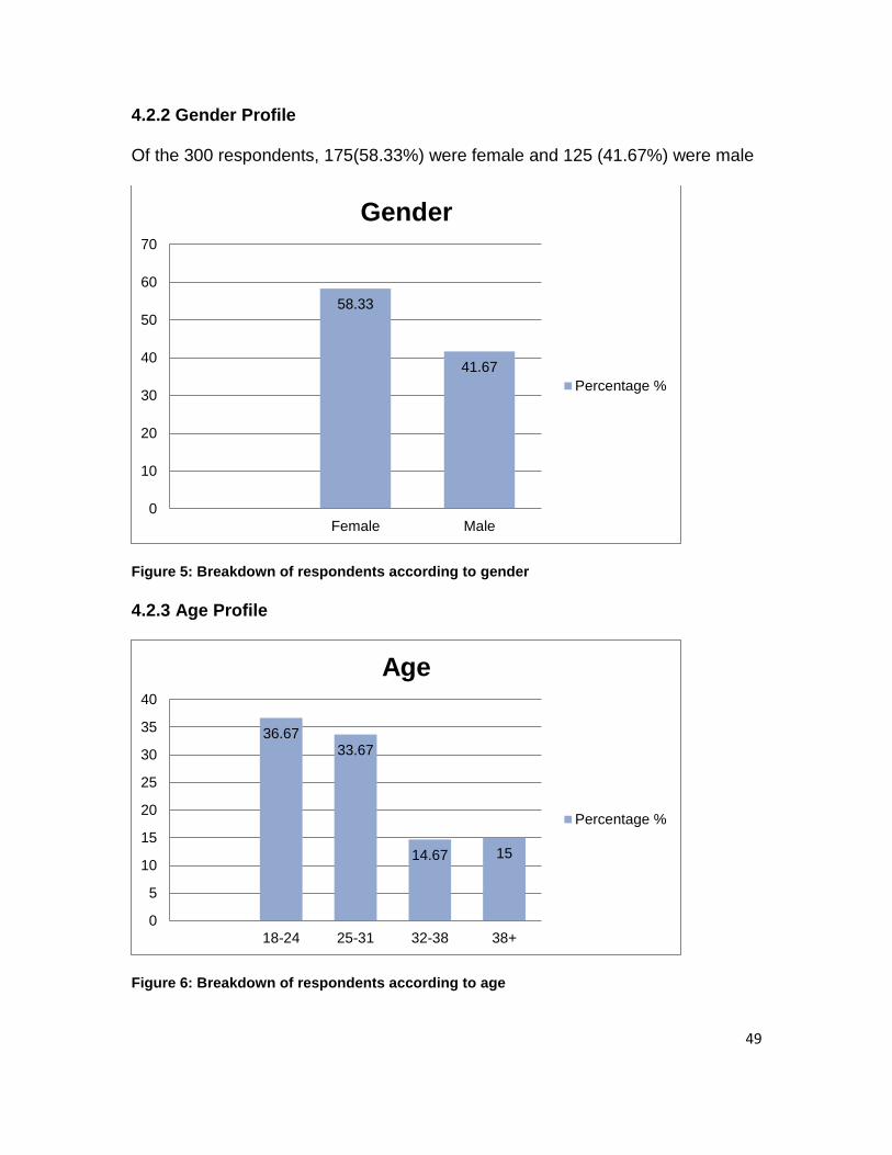
49

4.2.2 Gender Profile Of the 300 respondents, 175(58.33%) were female and 125 (41.67%) were male

Figure 5: Breakdown of respondents according to gender

4.2.3 Age Profile

Figure 6: Breakdown of respondents according to age

58.33

41.67

0

10

20

30

40

50

60

70

Female Male

Gender

Percentage %

36.67 33.67

14.67 15

0

5

10

15

20

25

30

35

40

18-24 25-31 32-38 38+

Age

Percentage %

50

The majority of the respondents were between the ages of 18-24. This age group

accounted for 110 respondents (36.67%), followed by 101 (33.67) respondents of

ages 25-31. In fact, respondents between the age 18-24 and 25-31 accounted

for 70.33% of the respondents. The group 38+ had 45 respondents (15%) and

finally 32-38 years had 44 respondents (14.67%).

Because the legal drinking age in South Africa is 18, all respondents were 18 and

above.

4.2.4 Marital status Profile

As displayed in Figure 5, 76% of respondents (228) were single; 60 respondents

(20%) were married; 2 respondents (0.67) were widows and 10 (3.33%)

respondents were either separated or divorced.

Figure 7: Breakdown of respondents according to marital status

76

20

0.67 3.33 0

10

20

30

40

50

60

70

80

Sin

gle

Ma

rrie

d

Wid

ow

Sepe

rate

d/D

ivorc

ed

Marital Status

Percentage %

51

4.2.5 Educational Level Profile

As displayed in Figure 8, the majority of the respondents (176 which translates to

58.67%) had either a Bachelor’s or an Honours degree, 85 respondents

(28.33%) had obtained a matric certificate, 29 respondents (9.67%) had either a

Master’s degree or a Doctorate. Finally, 10 (3.33%) had only reached high school

but had not completed matric.

Figure 8: Breakdown of respondent according to the level of education.

4.2.6 Alcohol consumption Profile

Figure 9 displays the number of respondents who either consume alcohol and

those who do not consume alcohol. From the sample, 204 respondents (68%)

consume alcohol and 96 respondents (32%) do not consume alcohol.

3.33

28.33

58.67

9.67

0

10

20

30

40

50

60

70

Hig

h S

choo

l

Ma

tric

De

gre

e/

Hono

urs

Ma

ste

rs/D

octo

rate

Educational Level

Percentage %

52

Figure 9: Respondents who consume alcohol versus respondents who don’t

4.3 Descriptive Statistics

Descriptive statistics are numerical values used to summarise and describe a

sample. Pattern can emerge from the data (Hebl, n.d.). The table below presents

descriptive statistics used for the study including the Mean, Standard Deviation

and Cronbach Alpha (APPENDIX G)

n= number of sample

µ=mean

σ= standard deviation

α= Cronbach alpha

Table 6: Descriptive statistics table

Construct N µ α Cronbach

Alpha

Personal Involvement 300 5.23 1.2 0.91

Trustworthiness 300 5.31 1.21 0.91

Expertise 300 5.4 1.16 0.91

Informational Transformational 300 3.45 0.85 0.85

68

32

0

10

20

30

40

50

60

70

80

Yes No

Alcohol consumption

Alcohol consumption

53

The mean is also known as the average. The highest mean with the four

constructs is the Expertise (5.4) and the lowest is informational transformational

with an average of 3.45.

The standard deviation is at its highest with trustworthiness (1.21) and lowest

with Informational Transformational. Informational Transformational data are

more concentrated around the mean. The standards deviation is defined as the

dispersion of the set of data from the mean (Rumsey, 2011).

As discussed in 3.8.2, the Cronbach alpha scores all met the research

requirement to be considered reliable and internally consistent. The acceptable

reliability score is 0. 7 (Nunnaly,1978).In this study the Cronbach alpha ranged

between 0.8470 – 0.9119.

4.4 ANOVA analysis

4.4.1 Multivariate Correlation

Table 7: Multivariate Correlation across all constructs

Constructs

Personal

involvement

Trustworthiness

Expertise

Informational

transformational

Personal

involvement

1.0000 0.3535 0.3327 -0.3597

Trustworthiness 0.3535 1.0000 0.5270 -0.3919

Expertise 0.3327 0.5270 1.0000 -0.3352

Informational

transformational

-0.3597 -0.3919 -0.3352 1.0000

Interpretation of correlation

0.15-0.29 means the correlation has a small effect size

0.30-0.49 means the correlation has a medium effect size

54

0.50 and above mean the correlation has a large effect

From the table, there is a positive relationship between Personal Involvement

and Trustworthiness; Personal Involvement and Expertise; and Expertise and

Trustworthiness.

The medium-effect size results (0.3535) in Personal involvement and Expertise

suggest that respondents’ trust in the sponsors led to involvement in the advert. It

is also true that personal involvement was interrelated to perceived expertise of

the sponsor with a medium-effect size of 0.3327. Respondents also trusted the

advertisement because of the perception that the sponsor/s was/were experts.

The correlation with Expertise and Trustworthiness was high at 0.5270.

To determine if the mean of the constructs differed significantly (between

categories of the demographic variables) and if further relationships between the

constructs and the demographics exist, ANOVA will be used. ANOVA (analysis

of variance) is a collection of statistical models with associated procedures. The

below will also use MANOVA which is an ANOVA with several dependent

variables. The ANOVA tests for variation between 2 or more means (of a

category) whilst MANOVA tests variation between two or more vectors of means

(French, Macedo, Poulsen, Waterson & Yu, n.d.)

55

Overall mean scores of all constructs

Figure 10: Consolidated means with all the constructs and the 3 advert sponsor

The Figure 10 above and Table 8 below show the least square means produced

by the MANOVA analyses and are used for graphical presentation.

Table 8: Mean score of the 3 advert sponsors across the constructs

Advert

Sponsor

Personal

Involvement Trustworthiness Expertise

Informational

Transformational

BOTH 4.48 4.77 4.67 3.69

PADD 4.29 4.85 4.34 3.48

SAB 4.65 4.86 4.78 3.4

56

The study will investigate each construct to see where there is a significant

difference between the means of the construct and type of advert by using

ANOVA analyses.

Table 9: ANOVA table with respect to SAB, PADD and Both (Partnership) and constructs

Advert Sponsor: SAB,PADD and Partnership with Both

Constructs Df F-Ratio p-value

Personal Involvement

299 2.06 0.1288

Trustworthiness 299 0.855 0.4263

Expertise 299 4.79 0.0089

Informational Transformational

299 4.4 0.0131

The significant differences are noted in Expertise (0.0089) and Informational

(0.0131), and Transformational where the p-value <0.05. This suggests that the

adverts were perceived to be sponsored by experts and respondents gained

useful information from them.

Post hoc Multiple comparison tests (Tukeys HSD) were done to assess where

significant differences exist. The ANOVA letter group shows the mean scores

and groups them for levels of significance. The levels not connected by the same

letter have a significant difference.

ANOVA connecting letters report for overall difference of means for Personal

Level.

Table 10: ANOVA connecting letters for overall difference of means for Personal

Involvement across the 3 sponsored adverts

Level Mean

SAB A 5.39

BOTH (Partnership) A 5.25

PADD A 5.05

57

From Table 10, it is clear that there is no significant difference in the mean

scores of personal involvement across SAB, PADD and with the partnership

between both. This confirms what was shown in Table 8.

Table 11: ANOVA connecting letters for overall difference of means for Trustworthiness

across the 3 sponsored advert

Level Mean

SAB A 5.40

PADD A 5.34

BOTH(Partnership) A 5.18

Table 11 shows no significant difference between trustworthiness across SAB,

PADD and with the partnership between both. This confirms what is reported on

table 8.

ANOVA connecting letters report for actual total difference with means for

Expertise.

Table 12: ANOVA connecting letters report for actual total difference with mean for

Expertise.

Level Mean

SAB A 5.62

BOTH (Partnership) A B 5.46

PADD B 5.13

With regards to Expertise, a significant difference is seen between SAB and

PADD. Respondents regarded SAB to be more of experts and PADD to be least

of experts. The partnership shows higher mean levels than PADD but less than

SAB.

58

Table 13: ANOVA connecting letters report for actual total difference with means for

Informational Transformational

Level Means

BOTH (Partnership) A 3.64

PADD A B 3.41

SAB B 3.29

Table 13 indicates a significant difference between the partnership with both and

SAB with regards Informational Transformational.

Respondents got more informational or found the advert to be informative when

the partnership between both was used. Respondents gained the least

information when SAB sponsored the advert.

4.4.2 Demographics and ANOVA 4.4.2.1 Race and ANOVA

Figure 11: Consolidated mean scores for constructs and the races

59

Table 14: Mean scores for each construct against the race groups

Personal

Involvement

Trustworthiness

Expertise

Informational

Transformational

content

1. Asian 4.87 5.28 4.80 3.55

2. Black 4.66 4.70 4.76 3.27

3. Coloured 3.93 4.58 4.26 3.62

4. White 4.41 4.71 4.57 3.65

Figure 11 and Table 14 show the means of the race groups. Trustworthiness,

Personal Involvement and Expertise are higher with Asian respondents.

ANOVA will further explain the extent of the differences.

Table 15: ANOVA analysis for constructs and race groups

Race Groups

Constructs Df F-Ratio P-value

Personal Involvement

299 2.39 0.07

Trustworthiness 299 1.99 0.11

Expertise 299 1.03 0.38

Informational Transformational content

299 1.9416 0.12

The ANOVA shows no significant difference between the means for Involvement,

trustworthiness, expertise and informational transformational content within the

race.

60

4.4.2.2 Gender and ANOVA

Figure 12: Consolidated mean scores of construct and gender

Table 16: Mean scores for each construct against the gender

Personal

involvement

Trustworthiness

Expertise

Informational

Transformational

content

1. Female 4.58 5.01 4.65 3.45

2. Male 4.36 4.62 4.54 3.59

The above mean scores show marginal difference between female and male

respondents. The table below will check for significant differences.

61

Table 17: ANOVA analysis of construct and gender

Gender

Constructs Df F-Ratio P-value

Personal Involvement 299 2.39 0.07

Trustworthiness 299 4.33 0.04

Expertise 299 0.003 0.96

Informational Transformational

299 0.3497 0.5547

The only significant difference noted here is within trustworthiness. Females are

more trusting of the advertisement then males.

4.4.2.3 Age and ANOVA

Figure 13: Consolidated mean scores of construct and age

62

Table 18: Mean score between construct and age groups

Personal

involvement

Trustworthiness

Expertise

Informational

Transformational

content

1:18-24 4.28 4.62 4.45 3.75

2: 25-31 4.45 4.75 4.50 3.68

3:32-38 4.35 4.76 4.50 3.43

4: 38+ 4.79 5.14 4.95 3.22

The table suggests that older persons (38+) are more trusting; more involved and

perceive sponsors to be experts. The younger the respondents, the higher the

means scores for informational transformational content. This suggests that

younger people found the advert to be more informative and useful than older

respondents.

The AVONA analysis table will interpret whether the difference are significant.

Table 19: AVONA analysis between constructs and age

Age

Constructs Df F-Ratio p-value

Personal Involvement 299 2.57 0.054

Trustworthiness 299 0.47 0.7

Expertise 299 1.34 0.26

Informational Transformational content

299 4.47 0.004

The p-value of Personal involvement is 0.054, which is marginally higher than the

required acceptable score of 0.05 and less. The only significant difference is

between the age and informational transformational content. Younger

respondents found the advert to be more informative than older respondents.

63

4.4.2.4 Marital status and ANOVA

Figure 14: Consolidated mean scores of construct and marital status

Table 20: Means score of constructs and marital status

Personal

involvement

Trustworthiness

Expertise

Informational Transformational

content

1: Single 4.91 5.29 5.08 3.59

2: Married 5.12 5.45 5.22 3.62

3: Widow 2.72 3.35 2.93 3.68

4:Seperated/Divorce

5.14 5.18 5.16 3.19

Mean scores of informational transformational content are low across of the

range of respondents. It is also clear that married respondents scored higher on

trustworthiness and expertise. The ANOVA analysis below investigates where

the difference is significant.

64

Table 21: ANOVA analysis between constructs and marital status

Marital Status

Constructs Df F-Ratio p-value

Personal Involvement 299 2.63 0.0498

Trustworthiness 299 1.86 0.14

Expertise 299 2.22 0.09

Informational Transformational

299 2.39 0.07

The analysis suggests that the only significant difference is in Personal

Involvement. Separated/Divorced respondents were more involved (5.14)

followed by Married respondents (5.12).

4.4.2.5 Level of Education and ANOVA

Figure 15: Consolidated mean scores of construct and level of education

65

Mean and Level of education

Table 22: Mean scores with construct and levels of education

Personal

involvement

Trustworthiness Expertise

Informational Transformational content

1. High School

3.69 4.82 3.80 3.56

2. Matric 4.62 5.21 5.02 3.40

3. Degree /Honours

4.62 4.80 4.80 3.53

4. Master /Doctorate

4.96 4.44 4.79 3.59

The more educated the respondents, the more involved they are. Respondents

with high school and matric were more trusting of the advert sponsor. The

ANOVA analysis was used to determine if the differences were significant.

Table 23: AVONA analysis and educational level

Education level

Constructs Df F-Ratio P-value

Personal Involvement 299 2.67 0.048

Trustworthiness 299 3.6 0.01

Expertise 299 2.41 0.06

Informational Transformational

299 0.04 0.99

The significant values are noted with Personal Involvement (0.048) and

Trustworthiness (0.01). The more trusting respondents were those with matric

and the least trusting were respondents with Masters degrees or Doctorates.

66

4.4.2.6 Consume alcohol and do not consume alcohol and ANOVA

Figure 16: Consolidated mean scores of construct and consume alcohol and those who do

not

Table 24: Mean scores for those who consume and those who do not consume alcohol

Personal

involvement

Trustworthiness

Expertise

Informational

Transformational

content

1. Yes, I

consume alcohol

4.62 4.93 4.69 3.35

2. No, I don’t

consume alcohol

4.32 4.71 4.50 3.69

Respondents that consume alcohol had higher mean scores on all mean scores

except Informational Transformational content.

67

Table 25: AVONA analysis for those who consume alcohol and those whose who do not

consume alcohol

Consume alcohol and don’t consume alcohol

Constructs Df F-Ratio P-value

Personal Involvement 299 0.17 0.68

Trustworthiness 299 0.33 0.56

Expertise 299 0.008 0.93

Informational

Transformational 299 3.76 0.054

Though the mean scores of those that consume alcohol are higher, there is no

significant difference in any of the constructs.

68

Using the SAS (APPENDIX H), the next session of the statistics will look at the level

of the construct with regards to respondents (low, medium and high) and Chi-

square. The Chi-square test is used to test independence and goodness of fit in

statistics. Independence testing determines if two or more constructs or variables

in two populations are dependent on each other. Good to fit testing determines if

the variable or constructs frequency distribution equals a theoretical frequency

distribution.

4.5 Personal Involvement results

Table 26: Degree of Personal involvement

Table of Personal Involvement scale

Advert Sponsor

Degree of Involvement

High involvement

Low involvement

Medium involvement

Total

Both 31 8 61 100

31% 8% 61%

PADD 27 10 63 100

27% 10% 63%

SAB 45 8 47 100

45% 8% 47%

Total 103 26 171 300

34.33% 8.67% 57% 100

Section B of the questionnaire comprised 13 descriptive words or scales to

measure persons’ interest or involvement in the issue being addressed by the

advertisement. It was then possible to determine where people had high, medium

or low involvement. The total sample was 300; 100 completed the SAB

sponsored advert, 100 completed the PADD-sponsored advert, while another

100 completed the advert sponsored by a partnership with both.

69

Scores between 13 –45 would be respondents with low involvement; 46–72

scores would have medium respondents and finally anything between 72–90

have high involvement. . Involvement is a motivational concept which is partly

reliant on a person’s needs and values (Zaichkowsky, 1987).

Both: These respondents participated in the study and answered the

questionnaire with an advert displaying partnership between SAB and PADD;

31% of respondents of the questionnaire with both logos had high levels of

involvement; 61% of respondents had medium involvement; 8% had low

involvement. Respondents with high personal involvement score high in finding

the advert to be important, interesting, beneficial, needed and fundamental.

These respondents find the advertisement extremely important in addressing the

issue of drunk driving.

PADD: These respondents answered the questionnaire with the advert

displaying the PADD logo; 27% of respondents of the questionnaire with the

PADD had high levels of involvements; 63% of respondents had medium

involvements and 10% had low involvement. PADD had the lowest high-involved

number of the three (both with 31% and SAB with 45%). PADD also had 10%

respondents with low involvement (which was the highest amongst the three

adverts). This means the respondents found the advert boring, unimportant,

uninteresting and meant nothing to them.

SAB: Respondents answered a questionnaire with the advert displaying the SAB

logo. Of the 100 respondents completing this particular SAB-sponsored advert,

45% had high involvement, 47% had medium involvement and 8% had low

involvement. SAB had the most respondents within the highly involved group.

These respondents had a personal connect or were able to bridge experience to

the advert (Krugman, 1965).

70

Table 27: Chi square and Personal Involvement

Statistic Value P-value

Chi-square 8.1782 0.0853

Likelihood Ratio Chi-square 8.0946 0.0882

The above Chi-square is used to determine whether involvement and the

different advertisement are independent from each other or not. By statistical

convention, we use the 0.05 probability level as our critical value and anything

above it proves that the variables are not correlated and anything below shows

correlation. The Chi-square is 0.0853.

4.6 Trustworthiness and Expertise results

Trustworthiness

Table 28: Degree of trustworthiness

Table of Trustworthiness

Advert Sponsor

Degree of Trustworthiness

High trustworthiness Low trustworthiness

Medium trustworthiness

Total

Both 47 6 47 100

47% 6% 47%

PADD 50 4 46 100

50% 4% 46%

SAB 51 11 38 100

51% 11% 38%

Total 148 21 131 300

49.33% 7% 43.67% 100

71

Section C of the questionnaire comprised two 5-semantic differential items

scored by a 7-point scale. The items are summed up to determine the level of

Trustworthiness and Expertise. The results were obtained by using SASS. The

study aimed to understand if trust of any of the organisations would be higher.

The audience would need to believe that the sources are genuine and that they

can trust the message.

Both: Of respondents of the questionnaire with both logos 47% showed high

trust in the source sponsoring the advertisement; 47% of the respondents had

medium trust and 6% had low trust. Trust for the partnership is 47% which is the

lowest when compared to SAB and PADD. This can be because the public might

perceive the NGO as losing focus by partnering with the same corporates that

they need to be boycotting. Pursuing partnerships and building close working

relationships with corporates by NGOs might distract them from fulfilling the

mission and using disruptive actions like protests (which could be effective)

against the organisation (Baur & Schmitz, 2011). Six percent of the respondents

did not trust the sources completely

PADD: Of respondents of the questionnaire with PADD logo 50% showed high

trust in the source sponsoring the advertisement; 46% had medium trust and 4%

had low trust. NGOs are viewed to not have a hidden agenda because they do

not commercially benefit from this. PADD only had 4% of the respondents who

perceived PADD as insincere and undependable.

SAB: Fifty-one percent of respondents of the questionnaire with the SAB logo

showed high levels of trust in the source sponsoring the advertisement; 38% of

respondents had medium trust and 11% had low trust. Over half of the

respondents who completed the advert with the SAB logo found them to be

trustworthy in addressing drunk driving. The number is contradictory to Szykman,

Bloom & Blazing (2004) who wrote that depending on advertising context, it

would be advantageous for the message sponsor of a social marketing advert to

be endorsed by a non-commercial source (Szykman, Bloom & Blazing, 2004).

72

Table 29 : Chi-square and Trustworthiness

Statistic Value P-value

Chi-square 5.0045 0.2868

Likelihood Ratio Chi-square 4.9339 0.2941

The Chi-square for the independent variables (trustworthiness and the three

logos) is 0.29 which is higher than the critical 0.05 needed to establish a

relationship.

Expertise

Table 30: Level of Expertise

Table of Expertise

Advert

Sponsor

Level of Expertise

High expertise Low expertise Medium expertise Total

Both 51 7 42 100

51% 7% 42%

PADD 42 7 51 100

42% 7% 51%

SAB 62 6 32 100

62% 6% 32%

Total 155 20 125 300

51.67% 6.67% 41.67% 100

Both: Of the respondents in the questionnaire with both logos 51% regarded the

source of the advertisement to have a high level of expertise in addressing the

social issue; 42% of respondents regarded that source as having medium

expertise, and 7% regarded the sponsors as having low expertise. Over half of

the respondents perceived the partnership as being competent and

knowledgeable in addressing the pandemic of drunk driving.

73

PADD: Forty-two percent of the respondents in the questionnaire with the PADD

logo regarded the source of the advertisement as having a high level of expertise

in addressing the social issue; 51% of respondents regarded that source as

having medium expertise, and 7% felt that the sponsors had low expertise. Over

93% of the respondents perceived PADD to have above medium competence

and capability in addressing the social issue of drunk driving.

SAB: Sixty-two percent of respondents felt SAB was an expert in addressing the

drunk driving issue; 32% felt SAB had medium expertise and 6% felt the sponsor

had low expertise. Then 62% of the respondents perceived SAB to be qualified

and competent to address the drunk driving pandemic and 6% disagreed that

SAB are experts. The high personal involvement score is the highest amongst

the other two, which means more respondents perceived SAB as experts and

experienced.

Table 31: Chi-square and Expertise

Statistic Value P-value

Chi-square 8.3199 0.0805

Likelihood Ratio Chi-square 8.3771 0.0787

The Chi-square did not show a significant correlation between the variables and

can be viewed as independent of each other. The Chi-squared p-value is 0.0805,

which is higher than the statistical accepted standard of 0.05.

74

4.7 Informational and Transformational results

Table 32: Agree/Disagree and Informational and Transformational

Table of Informational & Transformational

Advert Sponsor Scale

Agree Degree Total

Both 33 67 100

33% 67%

PADD 47 53 100

47% 53%

SAB 37 63 100

37% 63%

Total 117 183 300

39% 61% 100

The table comprised 13 items or statements measured on a 6-point scale:

‘strongly agree' to ‘strongly disagree’. ‘Strongly agree’, ‘agree’ and ‘somewhat

agree’ were grouped under ‘Agree’. ‘Strongly disagree’, ‘disagree’ and

‘somewhat disagree’ were grouped under ‘Disagree’.

Both logos representing partnership: Thirty-three percent of the respondents

in the questionnaire with both logos agree that the advertisement was

informational and transformational; 67% of respondents disagreed; 33%

respondents perceived the advertisement content as relevant, factual and

important. The respondents also connected the advertisement to an actual

experience which means they are likely to recall the advert when they consume

alcohol.

PADD: Forty-seven percent of the respondents in the questionnaire with a PADD

logo agree that the advertisement was informational and transformational; .53%

of the respondents disagreed. Over half of the respondents did not believe in the

content and were likely to forget it. Those respondents do not believe the facts

75

are presented in a clear and logical manner such that respondents can be

confident in assessing the merit of the organisation.

SAB: Of the respondents in the questionnaire with a SAB logo 37% agree to the

advertisement being informational and transformational; 63% of the respondents

disagreed. The advertisement with the SABA logo had 63% disagreeing to its

message content relevance. If respondents do not recall the advert, they are

unlikely to take the social marketing message.

Informational and Transformational advertisement content

Questions 24, 26, 28, 30 and 34 address the informational element. Informational

advertisement is defined as an ad that provides respondents with factual,

relevant brand data in a clear and logical.

The table below compared the respondents’ level of involvement and questions

relating to informational advertisement content. Informational ad content is

defined as factual, logical and clear about the brand, service or idea being

presented (Puto & Well, 1984).

Question 24: I learnt something from this advertisement that I didn’t know

Table 33: Degree of involvement in informational question number 24

Table of scale by Informational

Construct Question 24

Agree Disagree Total

High involvement 50 53 103

48.54% 51.46%

Low involvement 8 18 26

30.77% 69.23%

Medium involvement 59 112 171

34.5% 65.5%

Total 117 183 300

39% 61% 100%

76

Respondents were asked if they learnt something the advertisement that they did

not know.

Fifty (48.54%) respondents agreed to learning something they did not

know from the advert also displayed high levels of involvement; 53

respondents (51.46%) disagreed that they learnt anything from the

advertisement but showed high involvement.

One hundred and seventy-one respondents had medium involvement and

from those respondents 59 (34.5%) agreed to learning something from the

advert and 112 (65.5%) disagreed to learning anything.

Twenty six respondents had low levels of involvement and from those

respondents 8 (30.77%) learnt something from the advertisement and 18

(69.23%) disagreed to learning from it. This means that the majority of the

respondents knew that if they drank and drove, they could end up in jail

which was the massage on the advert.

Table 34: Chi-Square in the degree of involvement and informational question 24

Statistic DF Value P-value

Chi-Square 2 6.1375 0.0465

The above Chi-square is lower than the recommended 0.05. The study can

therefore conclude that there is a relationship between involvement and whether

the respondents learnt something from the advertisement. if the respondents feel

like they are learning from the advert, they are likely to be involved.

77

Question 26: There is nothing special about this advert that makes it different

from the others.

Table 35: Degree of involvement in informational question number 26

Table of scale by Informational

Construct

Question 26

Agree Disagree Total

High involvement 45 58 103

43.69% 56.31%

Low involvement 16 10 26

61.54% 38.46%

Medium involvement 111 60 171

64.91% 35.09%

Total 172 128 300

57.33% 42.67% 100

Of the 103 respondents with high levels of involvement, 45 respondents

(43.69%) agreed there was nothing special about the advertisement that

makes it different from the others and 58 (56.31%) disagreed.

From the 171 respondents with medium levels of involvements, 111

respondents (64.91%) agreed there was special about the advertisement

that makes it different from the others and 60 respondents (35.09%)

disagreed.

From the 26 respondents with low levels of involvements, 16 respondents

(61.54%) agreed there was special about the advertisement that makes it

different from the others and 10 respondents (38.46%) disagreed.

Table 36: Chi-Square in the degree of involvement and informational question 26

Statistic DF Value p-value

Chi-Square 2 12.0416 0.0024

78

The above Chi-square probability of 0.0024 is below the 0.05 which shows there

is a relationship.

Question 28: The advertisement was informative

Table 37: Degree of involvement in informational question number 28

Table of scale by Informational

Construct

Question 28

Agree Disagree Total

High involvement 81 22 103

78.64% 21.36%

Low involvement 9 17 26

34.62% 65.38%

Medium involvement 115 56 171

67.25% 32.75%

Total 205 95 300

68.33% 31.67% 100

High involvement: 81 respondents (78.64%) agreed that the advert was

informative and 22 respondents (21.36%) disagreed.

Medium involvement: 171 respondents were within the medium

involvement degree and of this group 115 (67.25%) agreed the advert was

informative whilst 56 (32.75%) disagreed.

Low involvement: A total of 26 respondents had low degrees of

involvement and from the 26, 9 agreed the advert was informative and 17

disagreed.

The Chi-square probability tabled below shows a strong relationship between

involvement and the extent to which the respondents found the advertisement

informative.

79

Table 38: Chi-Square in the degree of involvement and informational question 28

Statistic DF Value P-value

Chi-Square 2 18.8099 <.0001

Likelihood Ratio Chi-

Square

2 17.9344 0.0001

Question 30: If they could, the company(s) could provide evidence to support the

claim made on the advert.

Table 39: Degree of involvement in informational question number 30

Table of scale by Informational

Construct

Question 30

Agree Disagree Total

High involvement 87 16 103

84.47% 15.53%

Low involvement 22 4 26

84.62% 15.38%

Medium involvement 137 34 171

80.12% 19.88%

Total 246 54 300

82% 18% 100

High involvement: Of the 103 with a high degree of involvement,

87(84.47%) agreed that the company/s could provide evidence to support

claims made on the advert and 16 (15.53%) disagreed.

Medium involvement: Of the 171 respondents with medium levels of

involvement, 137 (80.12%) agreed to the question and 34 (19.88%)

disagreed

80

Low involvement: Of the 26 respondents with low involvements, 22

(84.62%) agreed that the company/s could provide evidence to support

claims made on the advert and 4 (15.58%) disagreed.

The Fisher’s Exact Test was used in this question instead of the Chi-square

because the Fisher's Exact Test is applied when one or more of your cells have

an expected frequency of five or less. From the above 4 in the low involvement

disagreed with the statement.

Table 40: Fisher’s Exact test and the degree of involvement and informational question 30

Fisher's Exact Test

Table Probability (P) 0.018

p-value 0.6295

The Fisher’s Exact Test had a p-value score of 0.6295. The score is higher than

0.05, which shows no relationship between the answers and the involvement.

Question 34: I can now accurately compare with other competing brands on

matters that are important to me.

Table 41: Degree of involvement in informational question number 34

Table of scale by Informational

Construct

Question 34

Agree Disagree Total

High involvement 62 41 103

60.19% 39.81%

Low involvement 7 19 26

26.92% 73.08%

Medium involvement 82 89 171

47.95% 52.05%

Total 151 149 300

50.33% 49.67% 100

81

High involvement: Of the 103 respondents in the high involvement group,

62 respondents (60.19%) that they could accurately compare the brand/s

on matters that are important to them and 41 respondents (39.81%)

disagreed.

Medium involvement: Of the 171 respondents with medium involvement,

82 respondents (47.95%) agreed to the statement and 89 (52.05%)

disagreed.

Low involvement: from the 26 respondents in the low involvement group, 7

agreed that they could accurately compare the brand(s) on matters that

are important to them and 19 respondents (73.08%) disagreed.

Table 42:Chi-Square in the degree of involvement and informational question 34

Statistic DF Value P-value

Chi-Square 2 10.0937 0.0064

The Chi-square p-value is 0.0064 which shows a relationship between the two

variables.

82

Questions 25, 27, 29, 31,32,33,35 and 36 address the transformational element.

A transformational advertisement is one that associates the experience of using

the advertised brand/s with unique psychological characteristics which would

typically not be associated with the brand experience to the same degree without

exposure of the advertisement.

Question 25: It is hard to give a reason, but somehow this advert is not really for

me.

Table 43: Degree of involvement in transformational question number 25

Table of scale by Transformational

Construct

Question 25

Agree Disagree Total

High involvement 31 72 103

30.1 69.9

Low involvement 17 9 26

65.38 34.62

Medium involvement 93 78 171

54.39 45.61

Total 141 159 300

47 53 100

High involvement: Of the 103 with high involvement, 31 (30.1%) agreed

that they could not give a specific reason, but the advert was not really for

them, and 72 (69.9%) disagreed.

Medium involvement: 171 respondents were in the medium involvement

group. From those respondents, 93 (54.39%) agreed that they could not

give a specific reason but the advert was not really for and 78 (45.61%)

disagreed.

83

Low involvement: Of the 26 with high involvement, 17 (65.38%) agreed

within that they could not give a specific reason, but the advert was not

really for them and 9 (34.62%) disagreed.

Table 44:Chi-Square in the degree of involvement and transformational question 25

Statistic DF Value P-value

Chi-Square 2 20.9312 <.0001

The p-value=0.001 indicates that the association is statistically significant at the

0.05 alpha level. There is a relationship between the degree to which

respondents were involved and the extent to which the respondents felt they did

not learn anything from the advert.

Question 26: This advert was meaningful to me

Table 45: Degree of Involvement for transformational question 26

Table of scale by Transformational

Construct

Question 27

Agree Disagree Total

High involvement 88 15 103

85.44% 14.56%

Low involvement 11 15 26

42.31% 57.69%

Medium involvement 125 46 171

73.1% 26.9%

Total 224 76 300

74.67% 25.33% 100

High involvement: Of the 103, 88 (85.44%) respondents say the advert

was meaningful to them and 15 (14.56%) respondents disagree.

84

Medium involvement: 125 (73.1%) respondents agreed that the advert

was meaningful to them and 46 (26.9%) disagreed.

Low involvement: Of the 26, 11 (42.31%) respondents say the advert was

meaningful to them and 15 (57.69%) respondents disagree

The below Chi-square p-value also reflects an association or relationship

between the two independent variables.

Table 46: Chi-Square in the degree of involvement and transformational question 27

Statistic DF Value P-value

Chi-Square 2 20.9312 <.0001

Question 29: I could really relate to this advert.

Table 47: Degree of involvement in transformational question number 29

Table of scale by SSec D_6 Transformational

Construct

Question 29

Agree Disagree Total

High involvement 78 25 103

75.73% 24.27%

Low involvement 10 16 26

38.46% 61.54%

Medium involvement 90 81 171

52.63% 47.37%

Total 178 122 300

59.33% 40.67% 100

High involvement: Of the 103 highly involved respondents, 78 respondents

(75.73%) agreed that they could relate to the advert and 25 (24.27%)

disagreed.

85

Medium involvement: Of the 171 medium involved respondents, 90

respondents (52.63%) agreed that they could relate to the advert whilst 81

( 47.37%) disagreed.

Low involvement: Of the 26 low-involved respondents, 10 (38.46%)

agreed they could relate to the advert and 16 (61.54%) disagreed.

Table 48: Chi-Square in the degree of involvement and transformational question 29

Statistic DF Value P-value

Chi-Square 2 19.3511 <.0001

Question 31: it is the kind of advert that keeps running through your head after

you’ve seen it.

Table 49: Degree of involvement in transformational question number 31

Table of scale by Transformational

Construct

Question 31

Agree Disagree Total

High involvement 65 38 103

63.11% 36.89%

Low involvement 8 18 26

30.77% 69.23%

Medium involvement 86 85 171

50.29% 49.71%

Total 159 141 300

53% 47% 100

High involvement: From the 103 respondents in this group, 65

respondents (63.11%) agree that this is the type of advert that keeps

running through ones head after seeing it and 39 (36.89%) disagree.

171 respondents are within the medium involved group. From the 171

respondents, 86 respondents (50.29%) agree to the question and 85

(49.17%) disagree.

86

From the 26 respondents in with low involvement, 8 agree that this was

the type of advert that keeps running through ones head after seeing it

and 18 (69.23%) disagree.

Table 50: Chi-Square in the degree of involvement and transformational question 31

Statistic DF Value P-value

Chi-Square 2 9.8853 0.0071

Question 32: If I could change my lifestyle, I would make it less like people that

consume alcohol.

Table 51: Degree of involvement in transformational question number 32

Table of scale by Transformational

Scale Question 32

Agree Disagree Total

High involvement 69 34 103

66.99% 33.01%

Low involvement 17 9 26

65.38% 34.62%

Medium involvement 82 89 171

47.95% 52.05%

Total 168 132 300

56% 44% 100

High involvement: 69 (66.99%) of highly involved respondents agreed to

the statement and 34 (33.01%) disagreed.

Medium involvement: 47 (47.95%) agreed that if they could they would

change their lifestyles to be less like people that consume alcohol and 89

(52.05%) disagreed.

Low involvement: 17 respondents (65.38%) within the low involvement

group agreed to the statement and 9 (34.62%) disagreed

87

Table 52: Chi-Square in the degree of involvement and transformational question 32

The Chi-square p-value of 0.0053 shows a relationship between the level of

involvement and willingness for respondents to change their lifestyles.

Question 35: When looking at the advert, I thought of how this might be useful to

me.

Table 53: Degree of involvement in transformational question number 34

Table of scale by Transformational

scale Question 35

Agree Disagree Total

High involvement 73 30 103

70.87% 29.13%

Low involvement 9 17 26

34.62% 65.38%

Medium involvement 103 68 171

60.23% 39.77%

Total 185 115 300

61.67% 38.33% 100

High involvement: Within the 103 highly involved respondents, 73

respondents (70.87%) thought of how the advert might be useful to them

and 30 (29.13%) disagreed

Medium involvement: Of the 171 respondents in the medium involvement

group, 103 (60.23%) agreed with the statement and 68 (39.77%)

disagreed that when they were exposed to the advert, they thought of how

it could be useful to them.

Statistic DF Value P-value

Chi-Square 2 10.4721 0.0053

88

Low involvement: From the 26 respondents within the low involvement

group, 9 respondents (34.62%) agreed to the statement and 17 (65.38%)

disagreed.

Table 54 below shows the Chi-square value as 0.0026 which is reveals a

relationship or correlation between the two variables.

Table 54:Chi-Square in the degree of involvement and transformational question 34

Statistic DF Value P-value

Chi-Square 2 11.8908 0.0026

Question 36: It is hard to put it in words, but this advert leaves me with a good

feeling about the brand/s.

Table 55: Degree of involvement in transformational question number 36

Table of scale by Transformational

scale Question 36

Agree Disagree Total

High involvement 84 19 103

81.55% 18.45%

Low involvement 10 16 26

38.46% 61.54%

Medium involvement 109 62 171

63.74% 36.26%

Total 203 97 300

67.67% 32.33% 100

89

High involvement: From the 103 high involved respondents, 84 (81.55%)

agreed that the advert left them with a good feeling about the brand (s)

and 19 (18.45%) disagreed.

Medium involvement: From the 171 medium involved respondents, 109

(63.74%) agreed the advert left them with a good feeling about the brand

(s) and 62 respondents (36.26%) disagreed.

Low involvement: 10 respondents (38.46%) agreed the advert left them

with a good feeling about the brand (s) and 16 (61.54%) disagreed.

Table 56: Chi-Square of the degree of involvement and transformational question 36

The Chi-square p-value shows a relationship or correlation between the degree

of involvement and feelings toward the brand after seeing the advert.

Statistic DF Value P-value

Chi-Square 2 20.4179 <.0001

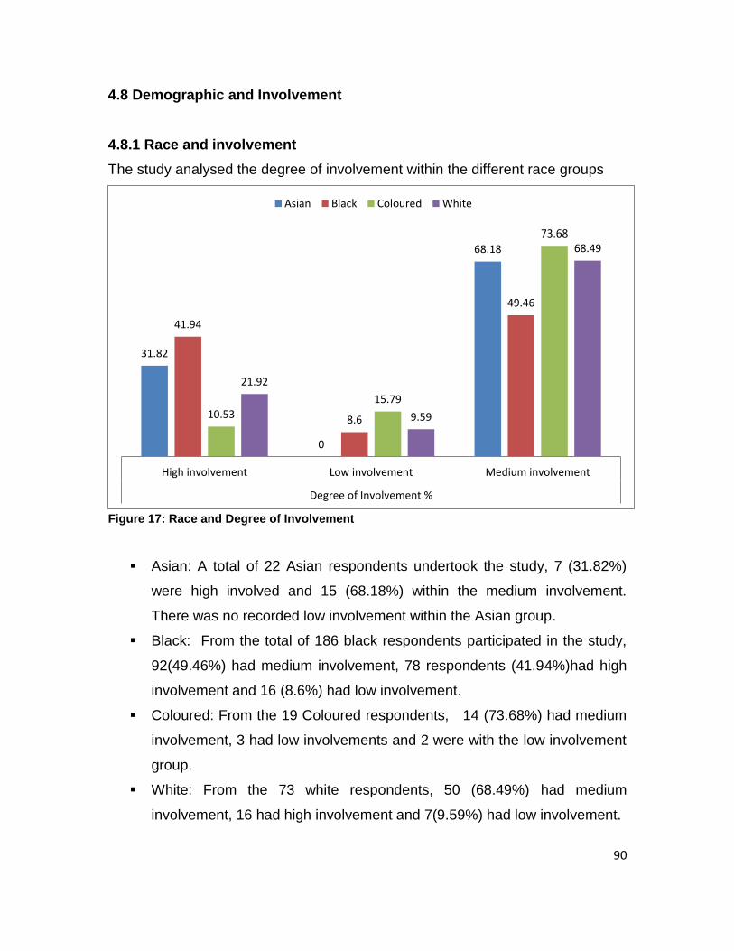
90

4.8 Demographic and Involvement

4.8.1 Race and involvement

The study analysed the degree of involvement within the different race groups

Figure 17: Race and Degree of Involvement

Asian: A total of 22 Asian respondents undertook the study, 7 (31.82%)

were high involved and 15 (68.18%) within the medium involvement.

There was no recorded low involvement within the Asian group.

Black: From the total of 186 black respondents participated in the study,

92(49.46%) had medium involvement, 78 respondents (41.94%)had high

involvement and 16 (8.6%) had low involvement.

Coloured: From the 19 Coloured respondents, 14 (73.68%) had medium

involvement, 3 had low involvements and 2 were with the low involvement

group.

White: From the 73 white respondents, 50 (68.49%) had medium

involvement, 16 had high involvement and 7(9.59%) had low involvement.

31.82

0

68.18

41.94

8.6

49.46

10.53

15.79

73.68

21.92

9.59

68.49

High involvement Low involvement Medium involvement

Degree of Involvement %

Asian Black Coloured White

91

The Chi-square indicates a relationship between the race and degree of

involvement with a Fisher’s exact test p-value of 0.0041. Fisher’s exact test was

used because some values were less than 5.

4.8.2 Gender and Involvement

Figure 18: Gender and Degree of Involvement

Females: 175 females participated in the study. From these females, 102

respondents had medium involvement, 59(33.71%) had high involvement

and 14 (8%) had low involvement.

Males: 125 females participated in the study. 69(55.2%) female

respondents had medium involvement, 44 (35.2%) had high involvement

and 12 (9.6%).

The Chi-square p-value was 0.8253 so there was no relationship between level

of involvement and gender.

33.71

8

58.29

35.2

9.6

55.2

High involvement Low involvement Medium involvement

Degree of Involvement %

Female Male

92

4.8.3 Age and Involvement

Figure 19: Age and Level of Involvement

The age groups were divided as follows:

18-24

25-31

32-38

38+

18-24: 110 respondents between the ages of 18-24 participated in the

study.68 (61.82%) had medium levels of involvement, 30 (27.27%) had

high involvement and 12 (10.91%) had low involvement.

25-31: 101 respondents between the ages of 25-31 participated in the

study.59 (58.42%) had medium involvement, 35(34.65%) had high

involvement and 7 (6.93%) had low involvement

32-38:44 respondents between the ages of 32-38 participated in the

study.27 (61.36%) had medium involvement, 14 (31.82%) had high

involvement and 3(6.82%) had low involvement.

27.27%

34.65% 31.82%

53.33%

61.82% 58.42%

61.36%

37.78%

10.91% 6.93% 6.82%

8.89%

18-24 25-31 32-38 38+

High involvement Medium involvement Low involvement

93

38+: 45 respondents were over the age of 38. 24 of the respondents over

38 (53.33%) had high involvement, 17 (37.70%) had medium involvement

and 4 (8.89%) had low involvement.

The Fisher’s Exact Test was used to determine if there was a relationship

between the age and level of involvement. The p-value was 0.0883 showed no

relation. (Please see APPENDIX H)

4.8.4 Marital Status and Involvement

Figure 20: Marital status and Level of involvement

Single: 228 single respondents participated in the study. From the single group,

133 respondents (58.33%) had medium involvement, 76 respondents (33.33%)

were within the high involvement and 19 (8.33%) had low involvement.

Married: 60 married respondents participated in the study. From the married

respondents, 30 (50%) had medium involvement, 24 respondents (40%) had

high involvement and only 6 respondents (10%) had low involvement

33.33

40

0

30

58.33

50 50

70

8.33 10

50

0

Single Married Widow Seperated/Divorced

High involvement Medium involvement Low involvement

94

Window: Only 2 respondents were widows,. 1(50%) had low involvement and the

other had medium involvement.

Separated or divorced: 10 respondents were either separated or divorced, 7

(70%) had medium involvement and 3 (30%) had high levels of involvement.

There was no significant relationship noted by the Fisher’s Exact Test between

the marital status and level of involvement. See Appendix

4.8.5 Educational level and Involvement

Figure 21: Educational Level and Level of Involvement

High School: 10 respondents were within the high school group. This

group did not complete their matric. From this group 7 respondents (70%)

had medium involvement, 2 (20%) had low involvement and 1 (10%) had

high involvement.

10

30.59

36.93 37.93

70

62.35

52.84

62.07

20

7.06 10.23

0

High School Matric Degree/Honours Masters/Doctorate

High involvement Medium involvement Low involvement

95

Matric: 85 respondents highest qualification was a matric. From this group,

53 (62.35%) had medium involvement, 26 respondents (30.59%) had high

levels of involvement and 6 respondents (7.06%) had low involvement.

Degree or Honours: 176 respondents had a diploma, degree or honours.

From this group, 93 (52, 84%) respondents had medium involvement, 65

(36.93%) had high involvement and 18 (10.23%) had low involvement.

Masters or Doctorate: 29 respondents had either a Masters or Doctorate.

From this group 18 respondents (62.07%) had medium involvement and

11 respondents (37.93) had high involvement.

There was no significant relationship between the educational level and level of

involvement. The Fisher’s Exact Test had a p-value of 0.1540.

4.8.6 Alcohol Consumption and Involvement

Figure 22: Alcohol consumption and involvement

From 204 respondents who consume alcohol, 113 respondents (55.39%)

had medium involvement, 72 (35.29%) had high involvement and 19

(9.31%) had low involvement

35.29

55.39

9.31

32.29

60.42

7.29

High involvement Medium involvement Low involvement

Involvement %

Yes No

96

From the 96 respondents who do not consume alcohol, 58 (60.42%) had

medium levels of involvement, 31 (32.29%) had high levels of involvement

and 7 (7.29%) had low levels of involvement.

The Chi-square p-value was 0.6810 does not indicate a relationship between

respondents who consume alcohol and those that don’t with the level of

involvement.

97

Chapter 5: Discussion of results

5.1 Introduction

This chapter discusses the results presented in Chapter 4 with alignment to

research questions posed in the literature review. The results will specifically

focus on the parts were statistically significant differences were noted amongst

the constructs and the demographics. This discussion will answer and make

clear of the factors affecting the effectiveness of social marketing advertising.

The chapter will also look at the different levels of each of the variables to better

understand where the most of the respondents rank.

5.2 Demographics

The demographic profile in the sample allowed for certain vigorous statistics but

was not equally distributed amongst the groups. Due to the random selection of

the respondents, some of the demographic groups are not richly represented.

This could be because the respondents were from Gauteng and primarily found

in universities. This does not compromise the quality of the data attained but

would be important to note if one would like to use the study to understand the

behaviour in another province.

5.2.1 Race profile

The breakdown of the respondents’ demographics is presented in Figures 4 to 7.

The breakdown shows that the majority of the respondents were Black

respondents who are also a majority race in South Africa followed by White

respondents. In 2013, black persons in South Africa represented 79.8% of the

population; white persons were 8.7% of total population; Coloured persons

represented 9% of total South Africa population and Asian people were 2.5%

(Statistics South Africa, 2013). Due to convenience sampling technique used to

acquire the sample, some of the races (Asians and Coloured) were poorly

98

presented. The difference in the sample could also be because most of the

respondents were from Gauteng.

5.2.2 Gender profile

The majority of the respondents were female, which is also true about the South

Africa population. The spread is fairly split between the genders allowing for

robust statistical study between the females and males.

5.2.3 Age profile

The respondents between the ages of 18-31 accounted for 70.33% of the study

as displayed in Chapter 4. The balance of the respondents was over the age of

32. The majority of the respondents were young persons. This is a particularly

good for the study because drunk driving is more prevalent among younger

persons so the statistical analysis will be relevant for younger persons.

It was also difficult to establish the age of persons 38+ because this is a wide

group, but the questionnaire did not categorise them, but instead all respondents

over the age of 38 fall in one category.

5.2.4 Marital status profile

A flaw in the study shows that the majority of the respondents were singles at

over 76%. This could mean the results are more meaningful to this group. If

further study is to be explored, it would be recommended that the focus also

adequately cover the married or divorced.

5.2.5 Educational level profile

The majority of the respondents were educated, with at least a degree. This

would make the study specifically relevant to the more educated. However, it can

also be useful to less educated respondents because they represent a third of

the study.

99

5.2.6 Consume alcohol versus do not consume alcohol

Respondents consuming alcohol were the majority of the respondent. This is

particularly important because the advertisements are targeted at those who

consume and might consider driving. It is not assumed that everyone consuming

alcohol engages in drunk driving; however, this group is more susceptible.

The study compares perception of both groups (consumers and those who do

not consume alcohol) to investigate if there is significant difference.

5.3 Results to research proposition 1:

The relationship between demographics and level of involvement

Figure 17 to Figure 21 depicts the relationship between demographics and level

of involvement in the advertisement. Levels of involvement are categorized as

(high, medium and low levels of involvement). These categories are formed by

adding the scores from the scale.

5.3.1 The relationship between Race and involvement

5.3.1.1 Introduction

Involvement amongst the races varied with Asian respondents ranking as the

most involved according to the overall mean score. This was followed by Black

respondents, White respondents were third and, finally Coloured respondents.

100

Figure 23: One way analysis of personal involvement relative to Race

The horizontal line running across or above the diamonds represents the mean

score of the race groups. The vertical endpoint represents the 95% confidence

interval of the mean. It is clear that Asian respondents (1) have a higher mean

score and the Coloured (3) has significantly lower as discussed above.

In terms of involvement level segments, figure 17 indicated that within the high

involvement group, Black persons had a higher percentage; within the medium

involvement group Coloured persons had a higher percentage and Coloured

respondents also had a higher percentage of people within the low involvement

group.

5.3.1.2 Discussion

Though the graph shows some differences between the race groups, the p-value

was used to determine the extent of the significance. The p-value of 0.07 (Table

15) shows no significant correlation between personal involvement and the race.

This means the personal involvement and race are independent from each other

and do not have a relationship. When Social marketers are designing advert and

want to increase involvement, race is not something they should focus on.

1 Asian

2 Black

3 Coloured

4 White

101

5.3.2 The relationship between gender and level of involvement

5.3.2.1 Introduction

Table 16 shows that females had a higher mean score than males. The graph

below shows that females (1) are marginally higher.

Figure 24: One way analysis of personal involvement relative to gender

Figure 17 depicts levels of involvement between females and males. Males have

a higher percentage in the high involvement segment (35.2%).Females have a

higher level of medium level of involvement with 58.29% respondents.

5.3.2.2 Discussion

Using the ANOVA analysis (table 21), the study does not reveal correlation

between the gender and level of involvement. The two variables are independent

from each other and do not have a relationship. Social Marketers must not

attempt to increase involvement by using gender. The chi-square test also did

not show any significance.

However, in table 21, the ANOVA analysis uncovers significant relationship

between the genders and trustworthiness. Though this was never part of the

proposition, it is important to note that females and males have different trust

levels and the two variables (trustworthiness and involvement) have a

1 Female

2 Males

102

correlation. Investigating what the trust triggers are in adverts addressing social

will ensure effectiveness and can affect design of social marketing advertisement

addressing drunken driving.

5.3.3 Age and involvement

5.3.3 The relationship between age and level of involvement

5.3.3.1 Introduction

The highest mean score was with the older respondents 38+. This was followed

by the age group 25-31.

Figure 25: One way analysis of personal involvement relative to age

The graph shows that respondents over the age 38(4) have a higher mean score

of 4.79 and 18-24 is lower (4.28).

Table 19 shows that 61.82% of the respondents within the ages 18-24 had

medium involvement; 58.42% of the 25-31 age group were also within the

medium involvement;61.36% of the 32-38 age group had medium involvement

and 53.33% in the 38 and above had high involvement. This indicates that the

older age group were likely to find the advertisement most relevant.

1 18-24

2 25-31

3 32-38

4 38+

103

5.3.3.2 Discussion

The ANOVA analysis does not confirm a significant relationship between the

involvement and age. It can be concluded that for persons to be involved in the

advert, it has nothing to do with age. The chi-square p-value of 0.0883 does not

indicate correlation between the age and the level of involvement. The variables

age and involvement are independent from each other.

However, table 19 showed a relationship between informational and

transformational content. This means that different age groups perceived the

content differently. From table 18, the study uncovers that age group 18-24

found the advert to be valuable, factual, logical and clear. These respondents

accept it as being verifiable. Those respondents are likely to connect the advert

to an experience therefore increasing recall. The older the respondents, the less

connection detected with the message content.

5.3.4 The relationship between marital status and level of involvement

5.3.4.1 Introduction

The mean score of married and separated/divorced respondents are higher at

5.12 and 5.14 respectively. The mean score for widows is relatively lower.

Figure 20 depicts married persons (40%) with the highest scores of involvement

towards the advertisement, single persons followed with 33.33%.

5.3.4.2 Discussion

The ANOVA analysis reveals a significant relationship between involvement and

the different marital status option. The study reveals that divorced respondents

and married respondents were more involved in the advert and widows were the

least involved. Though the study does not uncover the reasons for this, future

study must attempt to investigate the differences.

104

5.3.5 The relationship between educational level and level of involvement

5.3.5.1Introduction

Respondents with high levels education (Masters and Doctorate) had higher

means scores in involvement and the less educated respondents (high school)

have the least score (3.69)

Figure 26: One way analysis of personal involvement relative to educational level

From the graph, one can clearly see that master/doctorate (4) is higher and high

school (1) is relatively lower. Respondents with a degree or honours degree have

a higher mean compared to those with matric qualification. The mean scores

increases as the level of education increases.

Figure 21 depicts high involvement levels amongst respondents with masters

and doctorate (37.63%) followed by 36.93% from respondents with degrees and

honours.

5.3.5.2 Discussion

The ANOVA analysis shows significant difference between levels of education

and personal involvement (table 23). The more educated the respondents, the

more involvement showed towards advert. Those with masters/doctorate scored

1 High School

2 Matric

3

Degree/Honours

4 Masters

/Doctorate

105

the highest and those who finished in high school (without a matric) showed the

least involvement. Those with higher education levels perceive the advert to

have relevance. This is based on values, inherent needs and interests

(Zaichkowsky, 1985). This can be because those who are more educated

possibly have access to more information but it is important for social marketers

to be aware of this depending on who the adverts are targeting.

It is also important to note that trustworthiness and level of education had a

correlation. This is shown on table 23. Those who are less educated were more

trusting and skeptical behaviour is seen in the more educated respondents.

5.3.6 The relationship between those who consume alcohol/ those who

don’t and levels of involvement

5.3.6.1 Introduction

Respondents who consume alcohol had marginally higher mean scores

compared to respondents who do not consume alcohol.

Figure 27: One way analysis of personal involvement relative to those who consume

alcohol and those who don’t

1 Yes, I

consume

alcohol

2 No, I don’t

consume

alcohol

106

The above graph shows slight differences between those who consume alcohol

and those who don’t. From the 204 respondents who consume alcohol,

72(35.29%) had high involvement and of the 96 who did not consume alcohol 31

(32.29%) had high involvement as depicted in figure 22.

5.3.6.2 Discussions

The chi-squared showed there was no relationship between the variable so when

designing an advert addressing drunk driving, those who consume alcohol and

those who don’t are both involved.

The ANOVA analysis shows no significant difference between those who

consume alcohol and those that don’t consume alcohol and personal

involvement.

5.3.7 Conclusion

Wu (2001) recommends a framework that affects involvement which is presented

in the literature review. The framework recognizes personal and product factors

as attributes affecting involvement. Personal factors affecting involvement

include personal goals, needs and demographics (Wu, 2001)

From the study, it is revealed that demographics with close correlation to

involvement are level of education and marital status. The recognized

relationships will mean that if the social marketers want to increase involvement

for an advertisement addressing drunk driving, the level to which the target

audience is educated must be considered. The needs for the respondents differ

depending on education level. Personal involvement is affected by values,

interest and inherent need. It could be that the more educated perceive drunk

driving as more of an issue then the less educated.

The married and divorced were more involved and one could assume that this is

because of the level of responsibility amongst the married and divorced. This

assumption would need to be confirmed by future studies.

Race, age and gender did not show any relationship so the variables are

independent from each other.

107

5.4 Proposition 2

Source credibility comprises of both trustworthiness and expertise. The two are

however measured separately. Trustworthiness and expertise will be presented

for SAB, PADD and partnership. Firstly, the study will look at the overall picture

and then specifically to the advert sponsor.

Trust

Figure 28: One way analysis trustworthiness and the sponsors

The overall mean scores are shown above for trustworthiness. SAB appears to

be marginally higher than PADD and partnership slightly below.

Expertise

Figure 29: One way analysis expertise and the sponsors

108

SAB has higher mean scores as shown on the figure above followed by the

partnerships with regards to expertise.

5.4.1 People Against Drunken Driving (PADD) as a sponsor will have high

levels of credibility

PADD had the second highest mean scores in trustworthiness and the least

score in expertise. Szykman, Bloom and Blazing (2004) wrote that depending on

advertising context, it would be advantageous for the message sponsor of a

social marketing advert to be endorsed by a non-commercial source to increase

credibility (Szykman, Bloom & Blazing, 2004) This correlates with PADD scoring

high in the trustworthiness.

With regards to trustworthiness of PADD, 50% of the respondents have high level

trustworthiness and only 4% had low trustworthiness. 42% of respondents

perceived PADD to have high expertise which was the lowest amongst the 3.

5.4.2 Proposition 3

South African Breweries (SAB)-People Against Drunken Driving (PADD)

partnership sponsorship will have high levels of credibility

The partnership had the second highest expertise score and the lowest

trustworthiness score. Research done by Baur and Schmitz suggests that when

the partnerships are pursued, the public might perceive the NGO as losing focus

by partnering with the same corporates that they need to be boycotting against.

Pursuing partnerships and building close working relationship with corporates by

NGO’s might distract them from fulfilling the mission and using disruptive actions

like protests (which could be effective) against the organization (Baur & Schmitz,

2011).

From table 32, trustworthiness with co-sponsoring between SAB and PADD has

47% of the respondents were high levels of trustworthiness and 6% had low

trustworthiness. This indicates a less trustworthiness in the partnership

109

compared to PADD and SAB sponsored advertisement. However this is still a

positive relationship.

5.4.3 Proposition 4

South Africa Breweries (SAB) as a corporate sponsor will have less levels

of credibility

Table 28 shows 51% of respondents had high trustworthiness and 11% of

respondents (which was also the highest between the three advertisements) had

low trustworthiness scores. 62% of respondents were within the group that

perceived SAB to have high expertise levels.

SAB had the highest mean score in trustworthiness (4.86) and expertise (4.78).

In the literature review, Reih and Belkin (1998) suggest that consumers perceive

companies to be building brand image or awareness when addressing social

issues. This decreases sincerity of the message (Reih&Belkin, 1998). The

proposition is wrong and contradicts the literature. SAB is perceived as

trustworthiness and expert in addressing drunk driving.

5.4.4 Conclusion

There is no correlation between trustworthiness and the sponsors however there

is significant difference between expertise and sponsors (table 12).According to

this study, trustworthiness cannot be increased by selecting a particular sponsor

but if the Social marketer wants the audience to view an organisation as experts,

corporate (SAB) must be used independently or in the partnership.

The research also revealed significant relationship between the advert sponsors

and informational transformational (table 12). This means respondents found the

advert as factual, relevant, important and verifiable when the partnership was

sponsoring the advert with the likelihood to link the advert to an experience of

consuming. Strategic partnerships are beneficial for all sectors (private, public

and NGOs). Some of the benefits for the corporate include reputation

improvement (Flick & Heblich, 2007), product innovation and volunteerism. For

110

the NGO, advantages include resource support; improve awareness and

networking (Runte, 2009 as citedby Simpson, Lery & Tsarenko, 2011).If

respondents found the information to be more useful and more likely to connect it

to an experience when using partnership, it can be assumed that partnerships

will be more useful for this social issue.

5.5 Proposition 5 discussions:

The relationship between source credibility and level of involvement

The multivariate correlation table 7 shows a positive relationship with a medium

effect between personal involvement and trustworthiness (0.35); and personal

involvement and expertise (0.33). The below will look at the different source

credibility scores for the sponsors and levels of involvement.

5.5.1 The relationship between NGO (People Against Drunken Driving-

PADD) as the advertisement sponsor and level of involvement

Respondents were less involved in the advertisement sponsored by the NGO.

However, the score was still within the medium involvement category. PADD also

had the least mean score (4.29) amongst the three adverts. This could be

because PADD is an unknown NGO designed for the study. Respondents with

high involvement for PADD were 31%; 61% had medium involvement and 8%

had low involvement (as shown below)

111

Figure 30: Advertisement sponsor and Involvement

5.5.2. The relationship between the level of involvement and having both

SAB and PADD as an advert sponsor

Personal involvement had the second highest when the sponsors were both

PADD and SAB. Respondents found more relevance with the co-sponsoring

advertisement. This indicates that respondents had perceived relevance of the

advert based on inherent values, needs and interest when there was partnership.

From the respondents who completed the advert with a partnership, 27% were

highly involved; 63% had medium involvement and 10% had low involvement.

Respondents related to the message content positively in the partnership.

5.5.3 The relationship between the level of involvement and having SAB as

the primary sponsor

Forty-five percent of respondents were deemed to have high level of involvement

when SAB sponsored the advert which was the highest amongst the three; 47 %

had medium involvement and only 8% had low levels of involvement which was

the lowest amongst the three.

SAB had the highest score. Respondents were highly involved when SAB was

sponsoring the advert.

31%

61%

8%

27%

63%

10%

45% 47%

8%

High Involvement Medium Involvement Low Involvement

Advertisement sponsor and Involvement

Both PADD SAB

112

5.5.4 Conclusion

Though the overall p-value did not show a relationship between level of

involvement and the sponsors, SAB scored the highest and PADD had the least

mean scores. The variables are independent of each other. The developers of

the elaborated likelihood model suggest that regarding persuasion messaging,

advert audience give importance to the advertisement sponsor and the content

(Petty & Cacioppos, 1981).The study could not prove the relationship between

personal level and the sponsor but table 12 showed a positive correlation

between informational transformational advert content (message content) and

the sponsor.

5.6 Proposition 6:

The relationship between demographic and message content

(Informational and transformational content)

5.6.1 Race and Message content

Figure 31: Oneway analysis of content and race

1 Asian

2 Black

3 Coloured

4 White

113

5.6.1.1 Introduction

White respondents had the highest mean score with regards to content, followed

by Coloured respondents then Asian respondents and finally, Black respondents

had the least score. This can also be seen on the above figure 31.

5.6.1.2 Discussion

There was no detected relationship between race and message content. The two

variables are independent from each other.

5.6.2 Gender and Message Content

Figure 32: One analysis with message content and gender

5.6.2.1 Introduction

From the graph, it can be noted that the mean score of the males was higher

than that of the female respondents. Male respondents had an overall mean

score 0f 3.59 and females 3.45.

1 Female

2 Male

114

5.6.2.2 Discussion

The p-value of 0.5547 indicates that there was no correlation between the

message content and the gender demographic. The two variables are

independent and do not have a relationship.

5.6.3 Age and Message content

Figure 33: One way analysis between Age and Message Content

5.6.3.1 Introduction

From the summary graph, it is clear that there are differences in the age group.

The mean score seems to decrease as people get older. The mean score is

higher with age group 18-24 (3.75), followed by 25-31(3.68), then 32-38(3.43)

and finally 38+ (3.22).

5.6.3.2 Discussion

The p-value is used to see significant differences and correlation. As displayed in

Table 19, message content (informational and transformational ad content) and

age have p-value of 0.004. This means that as the age increased, people start to

view the information as less clear, logical, factual and relevant. The older the

respondents were, the harder it was to connect the advert to an experience. The

1: 18-24

2:25-31

3: 32-38

4:38+

115

social marketers must ensure that the messaging is age relevant and research

will need to be conducted so the message can relevant.

5.6.4 Marital Status and Message content

Figure 34: One way analysis between marital status and message content

5.6.4.1 Introduction

From the graph, it is clear that most participants were single and very few

widows. This could skew the data. Table 24 indicates that widows respondents

had the highest mean score (3.68), followed by married respondents wit 3.62.

Singles had the third highest (3.59) and finally separated or divorced with the

least score of 3.19.

5.6.4.2 Discussion

The p-value does not meet the statistical requirement to establish correlation

between the two variables. The two are independent from each other and when

design such advertisement for addressing drunk driving, the marital status is not

vital.

1: Single

2: Married

3: Widow

4: Separated or

Divorced

116

5.6.5 Level of Education and Message content

Figure 35: One way analysis of level of education and message content

5.6.5.1 Introduction

Those respondents with either a masters or doctorate had the highest mean

score (3.59) and the least score was of respondents with a Matric (3.40). The

figures are marginally apart.

5.6.5.2 Discussion

There was no correlation between the level of education of the respondents and

message content. The study can conclude that the variables are independent

and have no relationship.

1 High School

2 Matric

3 Degree/Honours

4 Masters

/Doctorate

117

5.6.6 Conclusion

Rhodes, Roskos-Ewolden, Eno and Monahan (2009) state that the effectiveness

of the advert is depended on the target audience characteristics and must be

matched with individual motivation (Rhodes, Roskos-Ewolden, Eno and

Monahan, 2009)

The study did show a relationship between message content and age. The

different age groups perceive the content on the advert differently. The younger

the respondent, the more likely the information was factual, relevant, important

and verifiable. The scale also measured transformational ad content which

indicates that the younger respondents would most likely connect the experience

of drinking alcohol to the advert with better recall.

However, there was no correlation with race, level of education, gender and

marital status

To the question, “Was the commercial informative”- there is a positive

relationship between the age and the extent to which the respondents found the

advert informative. It is therefore assumed that when addressing the issue of

drunk driving, the age specific information is important in the design.

The statement “I could really relate to the advert”, has a positive relationship with

age, educational level and between those we consume alcohol and those that do

not.

The statement “When looking at this advert, I thought of how it might be useful to

me” has a positive correlation. Across the age groups, the majority of the

respondents thought of how this could apply to them.

118

Proposition 7: The negatively framed message content has a high degree

of involvement.

The advert was negatively framed with the main message as “Don’t turn a good

time into doing time”- Regret nothing; don’t drink and drive

Table 7 depicting the multivariate correlations between the construct shows no

significant difference between personal involvement and message content. There

was a negative correlation score between the two constructs. This contradicts

what Tsai & Tsai (2006) wrote. The researchers suggest that negatively framed

messages were more effective than positively framed in the high involvement

arena.

The following chapter will summarise the findings and give recommendations.

119

Chapter 6: Conclusion and recommendation

6.1 Introduction

This chapter will conclude the study and present some recommendation for

future studies in advertising in social issues. The primary purpose of the study

was to understand the factors affecting advertising effectiveness in NGO-

corporate when addressing the drunken driving social issue

6.2 Conclusion of the study

The following were the research objectives that the study needed to address.

To conceptualize the factors that affect advertising effectiveness

The integration of the factors that affect advertising effectiveness in

NGO-corporate partnerships with the social issue of drunk driving

To determine the relationship between the factors and attitude towards

advertising effectiveness

To determine if the factors affecting advertising predict the attitude

towards advertising in NGO–corporate partnerships

To determine the difference between the factors that affect advertising and

attitude towards NGO–corporate with rigid variables (age, marital status,

education level).

From the literature review, the study was able to integrate factors affecting

advertising effectiveness. These included involvement, message content and

source credibility. Demographics also play a vital role in this type of advertising.

Demographics:

Race

Race did not have correlation with any of the constructs. It can be assumed that

race with personal involvement, source credibility and message content.

120

Gender

Females were found to be more trusting of the advertisement sponsor and

content and males were more sceptical. This is an important point to note

because it can be concluded that Females and Males have different trust

triggers. It will be for research to uncover what the trust triggers are so effective

adverts can be designed.

Age

Message content and age were correlated. The younger people seem to find the

information clearer, logical, important and could link it to an experience therefore

increase recollection of the advert. If Social marketers want to reach older

people, they would have to change certain messaging for the different

generations. A one size fits all approach would not be feasible.

Marital Status

The study showed correlation between involvement and marital status. The

married, divorced or separated were more involved in the advert than the singles.

Future research should attempt to understand why the married, divorced or

separated were more involved in the adverts. One could assume that because

they might have family and spouses, the advert content is important to increase

safety.

Level of Education

Level of education was correlated to personal involvement and trustworthiness.

The more educated respondents, the more involvement in the advert and the

less educated respondents had the least score. The study also uncovered that

the less educated respondents were more trusting of the source and the more

educated respondents were sceptical. This is vital for designing effective adverts

because though the less educated respondents were more trusting of the source,

they were not involved in the advert. Likewise, though the more educated

121

respondents were trusting, they were more involved in the presentation of the

content.

Those who consume alcohol and those who don’t

There was no correlation between those who consume alcohol and those who

don’t with any of the construct. The two groups’ perception on involvement,

source credibility and message content are not too significant.

Sponsors

SAB were regarded more qualified to address the issue of drunken driving

scoring higher in trustworthiness and expertise. Though the company has the

largest market share in alcohol sales in South Africa, respondents were more

favourable towards them.

Partnerships also show high levels of involvement compared to corporate

sponsored and NGO. SAB may consider partnering with credible NGOs when

addressing this because though the study shows that SAB is regarded as

experts, message content (informational and transformation ad content) is more

effective when there is a partnerships. This is important because people are

likely to recall the advert better and associate an experience with the advert

The partnership had a relationship with expertise. This could be because of the

SAB influence as PADD alone scored lower in the expertise. The partnership did

have correlation with message content. This means the content was perceived

as well presented, precise, logical and important.

The NGO, People Against Drunken Driving was made up for the sake of the

study. Even after this fact, respondents trusted them more than they trust the

partnership.

.

122

Constructs

When measuring the construct against each other, it is important to note that

personal involvement is affected by trustworthiness. People must trust the

sponsor to be involved in the advert and they must believe in the expertise of the

sponsor.

Though the following was not part of the proposition, the study also showed the

following

1. Trust levels differed within the two genders

2. Level of education also affected how people perceived the content.

3. More educated persons were less trusting.

Social marketers must also avoid advertisement that have a blanket approach

messaging across all age groups. The extent to which the different age groups

found the advert informative varied. The advertisers may have to design different

messaging for different age groups.

6.3 Recommendation and future research

The following are recommendations for future studies. Firstly, the study suggests

to get more valuable data, any future study must increase the sample size for

each advertisement. This will also allow for a wider demographic base. Secondly,

future studies must also use a credible NGO known by respondents. PADD was

a made-up NGO because of the lack of credible NGOs in the social issue of

drunk driving. Thirdly, the study primarily looked at drunk driving; futures studies

must use the same factors on a different social issue to examine if this will work

for social marketing in its entirety. Fourthly, the study showed that Married and

Separated/Divorce were more trust. Future studies must try to understand the

triggers that affect the trust element. This is important because drunk driving also

affects the wider population irrespective of marital status. Lastly, the study also

revealed that people with higher levels of education were more involved. In future

123

we must aim to understand what can drive more involvement across all people

and those less educated.

124

References

Abdulmajid, M. A. (2009) The Impact Of Source Credibility On Yemeni Male

Consumers' Attitudes Toward Print Advertisement, Brand Attitudes And

Purchase Intention Of Head Cover Product: The Moderating Role Of Brand

Familiarity, Doctoral dissertation, Universiti Sains Malaysia.

Acsinia, I.L. (2010), Theoretical and Applied Economics: Regulations and Best

Practices in Public and Non-profit Marketing, 9th International Congress of

International Association of Public and Non-profit Marketing, Bucharest,

Romania, National School of Political Studies and Public Administration,

Faculty of Public Administration

Alves, H. (2010) The Who, Where, and When of Social Marketing, Journal of

Nonprofit & Public Sector Marketing, Vol 22(4), pp.288-311

American Marketing Association (2013), Accessed 14 March 2014 from

www.ama.org/resources/Pages/Dictionary.aspx

Andreasen, A.R, (1995) Marketing Social Change: Changing Behaviour to

Promote Health, Social Development, and the Environment. San

Francisco: Jossey-Bass.

Andreasen, A.R, (2002) Marketing Social Marketing in the Social Change

Marketplace, Journal of Public Policy & Marketing: Spring 2002, Vol.

21(1), pp. 3-13.

Andreasen, R.A. and Kotler, P(2008) Strategic marketing for nonprofits

organization 7th edition Pearson Prentice Hall, Upper Saddle River

Arrive Alive (2012) Alcohol Breathalysers partners with AlcoSense for Southern

African Region, Accessed 3 November 2012, from

http://www.arrivealive.co.za/mobile/news.asp?NID=9019

125

Arrive Alive (2013) Drunk Driving and Road Safety, Accessed 8 November

2013, from

http://www.arrivealive.co.za/pages.aspx?i=1259#sthash.NKW5DA2Y.dpuf

Atkin, C.K. and Salmon, C. (2010) Communication campaigns in Berger, C.,

Roloff, M. and Roskos-Ewolden, D (Eds), Handbook of communication

science (2nd edition, pp.419-435), Thousand Oak, CA: Sage

Babbie, E. and Mouton, J. (2009) The practice of social research: South African

edition. Oxford University: Cape Town

Baker, M.J. (2003) The Marketing Book. 5th edition. Burlington MA: Butterworth-

Heinemann.

Baker, M.J. and Saren, M. (2010) Marketing Theory: The Student Text, Sage

Publications Ltd London

Bahari, S.F. (2010) Qualitative versus Quantitative Research Strategies:

Constructing Epistemological and Ontological Assumptions, Department

of Human Resource Development, Universiti Teknologi Malaysia

Baur, D. and Hans, P.S (2011) Corporations and NGOs: When Accountability

Leads to Co-optation, Journal of Business Ethics, Vol. 106, pp.9-21

Bearden, W.O., Netemeyer, R.G., and Haws, K.L. (2011) Handbook of marketing

scales: Multi-item measure for marketing and consumer behaviour

research, 3rd edition, Sage Publications, Thousand Oaks, Los Angles

Brenkert, G.G. (2002) Ethical Challenges of Social Marketing, Journal of Public

Policy & Marketing: Spring 2002, Vol. 21(1), pp. 14-25

Burn, C.A. and Bush, B.F (2010) Marketing Research, 6th edition,

Pearson/Prentice Hall

Cavill, N. and Bauman, A. (2004), Changing the way people think about health-

enhancing physical activity: do mass media campaigns have a role?,

Journal of Sports Sciences, Vol. 22(8)

126

Chang, C. (2012) Effectiveness of Consensus Information Advertising: The

Moderating Role of Situational Factors and Individual Difference, Journal

of Business & Psychology, Journal 27(4), pp483-494

Cismaru, M., Lavack, A.M , and Markewich, E (2009) Social Marketing

campaigns aimed at preventing drunk driving, International Marketing

Review, Vol. 26(3), pp. 292-311

Commission for global rad safety (2006), Make roads safe: A new priority for

sustainable development. Accessed 14 November 2013 from

http://www.arrivealive.co.za/documents/makeroadssafe.pdf

Cook, T.D. and Reichardt, C.S. (1979) Qualitative and Quantitative Methods in

Evaluation Research, , Beverly Hills, CA: Sage Publications

Cottea, J., Coulterb, R.A., and Moore, M (2005) Enhancing or Disrupting guilt:

the role of the ad credibility and perceived manipulative intent; Journal of

Business Research, Vol. 58, pp 361-368

Crossan, F.(2003) Issues in research: Research Philosophy: Towards an

understanding, Nurse Researcher. Vol. 11, (1)

Dash, K.N. (2005) Module: Selection of the research paradigm and methodology,

Accessed 21 November 2012 from

www.celt.mmu.ac.uk/researchmethods/Modules/Selection_of_methodoly/i

ndex

Donovan, R. (2011) Social marketing myth understandings, Journal of Social

Marketing, Vol. 1,(1), pp. 8-16

Dubihlela, J. (2011), Youth attitude towards advertisements depicting nudity and

alcohol: ethical dilemmas in advertising South African Journal of

Psychology, Vol. 41(2), pp. 207-217

Eisend, M. (2006), "Source Credibility Dimensions in Marketing Communication -

A Generalized Solution", Journal of Empirical Generalizations in Marketing

Science, Vol. 10(2)

127

Elder R.W., Shults, R.A., Sleet, D.A., Nichols, J.L., Thompson, R.S. and Rajab,

W. (2004) Effectiveness of mass media campaigns for reducing drinking

and driving and alcohol-related crashes: A systematic review, American

Journal of Preventive Medicine, Vol. 27(1) pp. 57-65

Falck, O. and Heblich, S. (2007) Corporate Social Responsibility: Doing well by

doing good, Journal of Business Horizons, Vol. 50(3), pp. 247-254,

Fragale, A.R. and Heath, C. (2004), Evolving informational credentials: The

(mis)attribution of believable facts to credible sources, Journal of

Personality and Social Psychology, Vol.30, pp. 225-236

French, A., Macedo, M., Poulsen, J., Wateron, T., and Yu, A. (n.d.)

Multivariate Analysis of Variance (MANOVA), Accessed 22 March 2014

from http://userwww.sfsu.edu/efu/classes/bio1710/manova/MANOVAnewest.pdf

Goldberg, F.S. (2011), Giving people what they want before they know they want

it, Vol. 48, pp. 117-122

Gordon, R, McDermott, L, Hastings, G. (2008), 'Critical issues in social

marketing: a review and research agenda', The Routledge Companion to

Nonprofit Marketing. Abingdon: Routledge, pp. 354-369.

Grube, J.W., and Wallack, L. (1994), Television beer advertising and drinking

knowledge, belief, and intention among schoolchildren, Journal of Public

Health, Vol. 84 (2), pp.254-259

Hair, J., Bush, R.P. and Ortinau, D.J. (2000), Marketing Research: A practical

approach for the new millennium. USA: McGrawhill

Haldermann, T. and Turner, J.W. (2009), Implementing a community-based

social marketing program to increase recycling. Social Marketing

Quarterly, Vol.15, (3), pp.114-127

Hall, V.D., Jones, S.C. and Iverson, D.C. (2011). "Consumer perceptions of

sponsors of disease awareness advertising", Journal of Health Education,

Vol. 111(1), pp.5 -19

Hassan, L.M., Walsh, G., Shui, E.M.K., Hastings, G. and Harris, F. (2007),

Modeling persuation in social advertising: A study of responsible thinking

128

in antismoking promotion in eight eastern EU ( European Union) member

states, Journal of advertising, Vol. 36(2), pp. 15-31

Halcomb, E.J. and Andrew, S. (2005) Triangulations as a method for

contemporary nursing research, Nurse research, Vol.13(2), pp.71-82

Hebl, M (n.d.) Descriptive Statistics, Accessed 22 March 2014 from

http://onlinstatbook.com/2/introduction/descriptive.html

Helmig, B. and Thaler, B. (2010) On the Effectiveness of Social Marketing –

What Do We Really Know?, Journal of Nonprofit & Public Sector

Marketing, Vol. 22, pp. 264-287

Hirschheim, R. (n.d.), Philosophy of Science and Research method is IS E.J

Ourso College of Business, Louisiana State University

Hope, K. and Waterman, H. (2003) Praiseworthy pragmatism? Validity and action

research, Journal of Advanced Nursing, Vol. 44(2), pp. 120-127

Hornik, R.C. (2002). Epilogue: Evaluation design for public health communication

programs. In Robert C. Hornik (Ed.), Public Health Communication:

Evidence for Behavior Change. Mahwah, NJ: Lawrence Erlbaum

Associates.

South African demographics 2013, Accessed 20 October 2013, from

http://www.indexmundi.com/south_africa/demographics_profile.html

Indu, R. and Jagathy Raj, V.P. (2012), Developing a Theoretical Framework for

a Study on the Impact of Advertising Credibility of Consumer Healthcare

Products, European Journal of Commerce and Management Research,

Vol. 1(1)

Kotler, P., and Roberto, E. L. (1989), Social marketing: Strategies for changing

public behavior

Kotler, P., Roberto, N., and Lee, N. (2002), Social Marketing: Improving the

Quality of Life. Thousand Oaks, CA: Sage

Kotler, P. and Zaltman, G. (1971) Social Marketing: An approach to planned

social changes, Journal of Marketing, Vol. 35, pp. 3-12

129

Kourula, A and Halme M (2008), Types of corporate responsibility and

engagement with NGOs: an exploration of business and societal outcome.

Vol. 8(4), pp. 557-570

Kumar, V., Rahman, Z., Kazmi, A. A. and Goyal, P. (2012) Evolution of

sustainability as marketing strategy: Beginning of new era, Journal of

Social and Behaviorial Science, Vol. 37, pp. 482-489

Krugman, H.E (1965) The impact of television advertising: Learning with

Involvement, Public opinion quarterly, Vol. 29, pp. 349-356

Levitt, S.D. and Porter, J. (2001) “How dangerous and drinking drivers?” Journal

of Political Economy, Vol. 109(6), pp.118-237

Majid, M.A. (2009), The impact of source credibility on Yemeni Male Consumers’

Attitude towards Print Advertisement, Brand Attitude and Purchase

Intention of Head Cover Product: The moderating role of Brand Familiarity.

Unpublished Thesis, Universiti Sains, Malaysia

Malhotra, N.K., Baalbaki, B.I, and Bechwati, N.N. (2010) Marketing Research: An

applied orientation Arab world edition England: Pearson

Marshall, M. and Oleson, A. (1994) “In the pink: MADD and public health policy in

the 1990s”, Journal of Public Health Policy, Vol.15(1), pp. 54-70

Martin, G. J. (2012), The Informational Content of Campaign Advertising.

Accessed on 14 November 2013, from

http://polisci.emory.edu/faculty/gjmart2/papers/GMartin_Advertising.pdf

Martin, E.J (2013), Trending Topic: How to Plan better ad campaigns and

support that planning, Accessed 12 December 2013, from

http://www.econtentmag.com/Articles/News/News-Feature/How-to-Plan-

and-Support-Better-Ad-Campaigns-92849.htm

McKay-Nesbitt, J. and DeMoranville, C.W. (2011) A strategy for advancing social

marketing, Journal of Social Marketing, Vol.. 2(1), pp. 52-69

Mounton, J. (2009) How to succeed in your Master’s and Doctorate studies: A

South African guide and resource book, Van Schaik: Pretoria

130

National Road Safety Strategy (2011), SA Road Safety Strategy 2011-2020:

Decade of action and Arrive Alive, Accessed 16 March 2014 from

www.arrivealive.co.za/documents/Road%20Safety%20Strategy%20for

%20South%20Africa%202011.pdf

Nunnaly, J. (1978) Psychometric theory. New York: McGraw-Hill

Ohanian, R. (1990), Construction and validation of a scale to measure celebrity

endorsers' perceived expertise, trustworthiness, and attractiveness,

Journal of advertising, Vol. 19(3), pp. 39-52.

Olie, R.L., Olffen, W., Berends, P. and Hendriks, W. (2005) The essential guide

to Masters Thesis in Organisation studies and strategy, Unpublished

Thesis Type, Maastricht University, Nederland

O’Shaughnessy, N. (1996) "Social propaganda and social marketing: a critical

difference?", European Journal of Marketing, Vol. 30 (10/11), pp.54 - 67

Park, T., Shenoy, R and Salvendy, G (2008) Effectiveness advertising on mobile

phones: a literature review and presentation of results from 53 case

studies; Behaviour & Information Technology, Vol. 27(5), pp. 355-373

Petty, R.E., and Cacioppo, J.T. (1981), Attitudes and Persuasion: Classic and

Contemporary Approaches. Dubuque, IA: William C. Brown Company

Publishers,

Phellas, C.N., Bloch, A. and Seale, C. (2011) Structured methods: interviews,

questionnaires and observations. Accessed 16 March 2014 from

www.sagepub.com/upm-data/47370_Seale_Chaper_11.pdf

Pongiannan, K. (2013) Relationship between social factors and the factors

affecting effectiveness of advertisement in print and electronic media- An

analytical study, Indian Steams Research Journal, Vol. 2(12)

Prochaska, J.O., and DiClemente, C.C. (2005), The trans-theoretical approach:

Handbook of psychotherapy integration, Vol. 2, 147-171.

Puto, C.P., and Wells, W.D. (1984), Informational and Transformational

Advertising: The Differential Effects of Time. Advances in consumer research,

Vol. 11(1).

131

Rajasekar, S., Philominathan, P. and Chinnathambi, V. (2006), Research

Methodology. Accessed 14 November 2013, from

www.scribd.com/doc/6949151/Research-Methodology

Rhodes, N., Roskos-Ewoldsen, D., and Eno, C.A. (2009) The content of cigarette

counter-advertising: Are the perceived functions of smoking addressed?,

Journal of Health communication, Vol. 14, pp. 658-673

Rice, R.E. and Atkins, C.K. (2013), Public communication campaigns: 4th edition,

Los Angeles: Sage publications Incorporation.

Rieh, S.Y., and Belkin, N. J. (1998), Understanding judgment of information

quality and cognitive authority in the WWW. In Proceedings of the 61st

annual meeting of the American society for information science, Vol. 35,

pp. 279-289

Rodgers, S. L.(2005) An Examination of Advertising Credibility and Skepticism in

Five Different Media using The Persuation Knowledge Model, In American

Academy of Advertising

Rumsey, D.J. (2011) How to Interpret Standard Deviation in a Statistical Data

Set. Accessed 22 March 2014, from http://www.dummies.com/how-

to/content/how-to-interpret-standard-deviation-in-a-statistic.html

Runte, M., Bassil, D. and Deshpande, S. (2009) Cause related marketing from

the Non-profits perspective: Classifying Goals and experienced outcomes:

Journals of Non-profit and Public Sector Marketing, Vol. 23(3), pp. 255

SADD: South African Against Drunk Driving (2013) Accessed 8 November

2013, from http://www.sadd.org.za/education/statistics

Segovia, J.B. (2013) Masking as a persuasive strategy in the adverting for

young, Journal of media education, Vol. XXL (41), pp 157-165

Sharma, M. (2007) Editorial: Social Marketing for Reduction in Alcohol Use,

Journal of Alcohol and Drug Education. Accessed 14 November 2013

from http://www.thefreelibrary.com/

Social+marketing+for+reduction+in+alcohol+use.-a0174101647

132

Sherif, M., and Hovland, C.I. (1961), Social Judgement. New Haven, CT: Yale

University Press.

Siegel, M. (1998) Mass Media Antismoking Campaigns: A Powerful Tool for

Health Promotion, American Society of Internal Medicine, Vol. 129, pp.

128-132

Simpson, D., Lefroy, K. and Tsarenko Y. (2011) Together and Apart: Exploring

structures of corporate-NPO relationships.

Smith, M.J. (1998) Social science in question London: Sage Publications

Statistics South Africa (2013), Mid-year population estimates. Accessed 25

March 2014 from

http://beta2.statssa.gov.za/publications/P0302/P03022013.pdf

Stead, M., Hasting, G., and McDenott, L. (2007) The meaning, effectiveness and

future of social marketing, Obesity review, Vol. 8(1), pp 189-193

Szmigin, I., Bengry-Howell, A., Griffin, Hackley, C. and Mistral, W. (2011) Social

Marketing individual responsibility and the “culture of intoxication:.

European Journal of Marketing, Vol. 45(5), pp. 759-779

Szykman, L.R., Bloom, P.N., and Blazing, J. (2004), Does corporate sponsor-

$hip of a socially oriented message make a difference? An investigation

of the effects of sponsorship identity on responses to an anti-drinking and

driving message. Journal of Consumer Psychology, Vol. 14, pp. 13-20.

Tajziehchi, S.(2011) Problems and challenging facing developing countries in

order to execute the social impact assessment of dams – a review,

European Journal of Scientific Research, Vol. 56, pp. 489-495

The Century Council (2009).Report: State of Drunk Driving Fatalities in the

American report .Virginia, Accessed 4 November 2012, from

www.centurycouncil.org.

Tipps, S.W., Berger, P.D., Weinberg, B.D. (2006) The effects of media

involvement on print media effectiveness, Journal of promotion

management, Vol. 12(2), pp. 54-75

133

Times LIVE (2009), Western Cape name and shame drunk driving campaign

'shut down, Accessed 1 February 2014, from

http://www.timeslive.co.za/politics/2013/06/13/ western-cape-name-and-

shame-drunk-driving-campaign-shut-down

Vallie, A. (2012) SAB grow market share and revenue, Accessed 5 October

2012, from

http://www.bdlive.co.za/articles/2011/11/18/ sab-grows-market-

shareandrevenue;jsessionid=298A58699A4D34A2010ACAC7AE5062DE.

present1.bdfm

Wang, A. (2009), "Cross-channel integration of advertising: does personal

involvement matter?; Journal of Management Research News, Vol. 32(9),

pp. 858 – 873

Wallack, L. (1990), Media advocacy: Promoting health through mass

communication. Health behaviour and health education: Theory, research,

and practice, pp. 370-386.

Welman, J.C. and Kruger, S.J. (2001) Research methodology: For the business

and administrative sciences, 2nd edition Cape Town: Oxford University

Press South Africa

Wheeler, R.T (2009), Non-profit Advertising: Impact of celebrity connection,

involvement and gender on source credibility and intention to volunteer

time or donate money, Journal of non-profit and public sector marketing,

Vol. 21, pp.80-107.

Williams, M. (2013), Name and shame the drunk drivers, Accessed 1 February

2014, from http://www.iol.co.za/motoring/industry-news/name-and-shame-

the-drunk-drivers-1.1531614

Wu, S.I. (2001) An experimental study on the relationship between consumer

involvement and advertising effectiveness. Asia Pacific Journal of

Marketing and Logistics, Vol. 13(1), pp.43-56.

134

Yeh, J.T. and Lin, C.L ( 2010) Measuring the effectiveness of the advertisement

sent via mobile phone: implications of the appeal, endorser, and

involvement model and purchasing behaviour, Social Behavior and

Personality. Vol. 38(2) pp 249-256

Zaichkowsky, J. (1994), The Personal Involvement Inventory: Reduction,

Revision and Application to Advertising. Journal of Advertising, Vol. XXIII

(4)

135

Appendix A: Advertisements

136

137

138

Appendix B : Scales

139

140

141

142

143

144

145

146

\

147

148

Appendix C: Questionnaire

SECTION A: Participants Information

1. Race

2. Gender

3. Age

4. Marital status

5. Educational level

6. Do you consume alcohol?

Asian

Black

Coloured

White

Female

Male

18-24

24-31

32-38

38+

Single

Married

Widow

Seperated/Divorced

High School

Matric certificate

Degree/Honours

Master/Doctorate

Yes

No

149

Please answer the below regarding the advertisement attached.

Directions:

To take this measure, you need to judge the advertisement against a series of descriptive words according

to how you perceive the advertisement attached. Here is how you are to answer.

If you feel that the advertisement is closely related to one end of the scale, you should place a cross as

follows

If you feel that the advertisement is closely related to one or the other end of the scale (but not extremely)

you should place your cross mark as follows

If you feel the advertisement seems on slightly related to one or the other end of the scale (but not really

neutral), you should place you cross as follow.

SECTION B: Personal Involvement

Work at fairly high speed through the next 13 questions. Do not worry or puzzle over individual items.

What is your first impression or immediate feeling of the advertisement attached?

important 1 2 3 4 5 6 7 Unimportant

important 1 2 3 4 5 6 7 Unimportant

important 1 2 3 4 5 6 7 Unimportant

1 important 1 2 3 4 5 6 7 unimportant*

2 of no concern 1 2 3 4 5 6 7 of concern to me

3 irrelevant 1 2 3 4 5 6 7 relevant

4 means a lot to me 1 2 3 4 5 6 7 means nothing to me*

5 useless 1 2 3 4 5 6 7 useful

6 trival 1 2 3 4 5 6 7 Fundamental

7 beneficial 1 2 3 4 5 6 7 nor beneficial*

8 uninterested 1 2 3 4 5 6 7 interested

9 significant 1 2 3 4 5 6 7 not significant*

10 vital 1 2 3 4 5 6 7 superfluous*

11 boring 1 2 3 4 5 6 7 interesting

12 essential 1 2 3 4 5 6 7 nonessential

13 not needed 1 2 3 4 5 6 7 needed

150

SECTION C (1): Trustworthiness

The next set of words will measure the extent to which you trust the source/company sponsoring the

advertisement

SECTION C (2): Expertise

The next set of words will measure the extent to which you regard the source to be an expert in addressing

the issue.

SECTION D: Informational and Transformational Ad content

The next 10 statements are structured differently. Please indicate to what extent you either strongly agree,

agree, somewhat agree, somewhat disagree, disagree or strongly disagree with the below statements

14 Undependable 1 2 3 4 5 6 7 Dependable

15 Dishonest 1 2 3 4 5 6 7 Honest

16 Unreliable 1 2 3 4 5 6 7 Reliable

17 Insincere 1 2 3 4 5 6 7 Sincere

18 Untrustworthy 1 2 3 4 5 6 7 Trustworthy

19 Not an Expert 1 2 3 4 5 6 7 Expert

20 Inexperienced 1 2 3 4 5 6 7 Experienced

21 Unknowledgeable 1 2 3 4 5 6 7 Knowledgeable

22 Unqualified 1 2 3 4 5 6 7 Qualified

23 Unskilled 1 2 3 4 5 6 7 Skilled

151

Thank you for your participation in this research initiative.

Regards, Luvhimba Taz Phaswana

24

I learned something from this advert that I didn't

know before about (this brand)

strongly

agree agree

somewhat

agree

somewhat

disagree disagree

strongly

disagree

25

It is hard to give a specific reason, but somehow

this advert is not really for me

strongly

agree agree

somewhat

agree

somewhat

disagree disagree

strongly

disagree

26

There is nothing special about this advert that

makes it different from the others

strongly

agree agree

somewhat

agree

somewhat

disagree disagree

strongly

disagree

27 The advert was meaningful to me

strongly

agree agree

somewhat

agree

somewhat

disagree disagree

strongly

disagree

28 The commercial was informative

strongly

agree agree

somewhat

agree

somewhat

disagree disagree

strongly

disagree

29 I could really relate to the advert

strongly

agree agree

somewhat

agree

somewhat

disagree disagree

strongly

disagree

30

If they could, the company could provide

evidence to support the claims made in the

advert

strongly

agree agree

somewhat

agree

somewhat

disagree disagree

strongly

disagree

31

It is the kind of advert that keeps running through

your head after you've seen it

strongly

agree agree

somewhat

agree

somewhat

disagree disagree

strongly

disagree

32

If I could change my lifestyle, I would make it

less like the people that use this brand/alcohol

strongly

agree agree

somewhat

agree

somewhat

disagree disagree

strongly

disagree

33 This brand fits my lifestyle very well

strongly

agree agree

somewhat

agree

somewhat

disagree disagree

strongly

disagree

34

I can now accurately compare with other

competing brands on matters that are important

to me

strongly

agree agree

somewhat

agree

somewhat

disagree disagree

strongly

disagree

35

When looking at the advert, I thought of how this

might be useful to me

strongly

agree agree

somewhat

agree

somewhat

disagree disagree

strongly

disagree

36

It is hard to put it in words, but this commercial

leaves me with a good feeling about the brand

strongly

agree agree

somewhat

agree

somewhat

disagree disagree

strongly

disagree

152

Appendix D: Multivariate and Cronbrach Alpha

Multivariate Correlations

Sec

A.1 2

Sec

A.2

Sec

A.3

Sec

A.4 2

Sec

A.5

Sec

A.6

Sec

A.7 2

Sec

A.8

Sec

A.9 2

Sec

A.10 2

Sec

A.11

Sec

A.12

Sec

A.13

Sec

A.1 2

1.00 0.55 0.53 0.57 0.51 0.36 0.47 0.54 0.50 0.56 0.31 -0.5 0.54

Sec

A.2

0.55 1.00 0.60 0.47 0.47 0.36 0.32 0.53 0.32 0.33 0.37 -0.3 0.48

Sec

A.3

0.53 0.60 1.00 0.41 0.55 0.38 0.36 0.45 0.38 0.35 0.33 -0.3 0.50

Sec

A.4 2

0.57 0.47 0.41 1.00 0.47 0.34 0.46 0.51 0.45 0.51 0.32 -0.5 0.39

Sec

A.5

0.51 0.47 0.55 0.47 1.00 0.47 0.53 0.57 0.41 0.41 0.39 -0.5 0.55

Sec

A.6

0.36 0.36 0.38 0.34 0.47 1.00 0.39 0.39 0.36 0.40 0.28 -0.4 0.40

Sec

A.7 2

0.47 0.32 0.36 0.46 0.53 0.39 1.00 0.45 0.59 0.56 0.33 -0.6 0.50

Sec

A.8

0.54 0.53 0.45 0.51 0.57 0.39 0.45 1.00 0.50 0.43 0.57 -0.4 0.56

Sec

A.9 2

0.50 0.32 0.38 0.45 0.41 0.36 0.59 0.50 1.00 0.70 0.33 -0.6 0.51

Sec

A.10 2

0.56 0.33 0.35 0.51 0.41 0.40 0.56 0.43 0.70 1.00 0.28 -0.7 0.53

Sec

A.11

0.31 0.37 0.33 0.32 0.39 0.28 0.33 0.57 0.33 0.28 1.00 -0.2 0.35

Sec

A.12

-0.5 -0.3 -0.3 -0.5 -0.5 -0.4 -0.6 -0.4 -0.6 -0.7 -0.2 1.00 -0.5

Sec

A.13

0.54 0.48 0.50 0.39 0.55 0.40 0.50 0.56 0.51 0.53 0.35 -0.5 1.00

153

Cronbach's α

α Plot Alpha

Entire set 0.8532

Excluded

Col

α Plot Alpha

Sec A.1 2 0.8305

Sec A.2 0.8351

Sec A.3 0.8346

Sec A.4 2 0.8354

Sec A.5 0.8317

Sec A.6 0.8427

Sec A.7 2 0.8361

Sec A.8 0.8303

Sec A.9 2 0.8354

Sec A.10 2 0.8361

Sec A.11 0.8438

Sec A.12 0.9070

Sec A.13 0.8330

154

Multivariate

Correlations

Cronbach's α

α Plot Alpha

Entire set 0.9070

Excluded

Col

α Plot Alpha

Sec A.2 Sec A.3 Sec A.5 Sec A.6 Sec A.8 Sec A.11 Sec A.13 Sec A.1 2 Sec A.4 2 Sec A.7 2 Sec A.9 2 Sec A.10 2

Sec A.2 1.0000 0.6018 0.4677 0.3560 0.5264 0.3727 0.4795 0.5471 0.4734 0.3175 0.3226 0.3343

Sec A.3 0.6018 1.0000 0.5518 0.3761 0.4489 0.3279 0.4954 0.5341 0.4084 0.3600 0.3828 0.3451

Sec A.5 0.4677 0.5518 1.0000 0.4699 0.5679 0.3868 0.5478 0.5094 0.4746 0.5315 0.4082 0.4124

Sec A.6 0.3560 0.3761 0.4699 1.0000 0.3938 0.2846 0.3951 0.3556 0.3384 0.3901 0.3569 0.3989

Sec A.8 0.5264 0.4489 0.5679 0.3938 1.0000 0.5710 0.5596 0.5425 0.5128 0.4502 0.4968 0.4260

Sec A.11 0.3727 0.3279 0.3868 0.2846 0.5710 1.0000 0.3544 0.3100 0.3226 0.3286 0.3328 0.2792

Sec A.13 0.4795 0.4954 0.5478 0.3951 0.5596 0.3544 1.0000 0.5385 0.3937 0.4981 0.5134 0.5339

Sec A.1 2 0.5471 0.5341 0.5094 0.3556 0.5425 0.3100 0.5385 1.0000 0.5750 0.4663 0.5045 0.5585

Sec A.4 2 0.4734 0.4084 0.4746 0.3384 0.5128 0.3226 0.3937 0.5750 1.0000 0.4564 0.4538 0.5088

Sec A.7 2 0.3175 0.3600 0.5315 0.3901 0.4502 0.3286 0.4981 0.4663 0.4564 1.0000 0.5864 0.5575

Sec A.9 2 0.3226 0.3828 0.4082 0.3569 0.4968 0.3328 0.5134 0.5045 0.4538 0.5864 1.0000 0.7035

Sec A.10 2 0.3343 0.3451 0.4124 0.3989 0.4260 0.2792 0.5339 0.5585 0.5088 0.5575 0.7035 1.0000

155

Excluded

Col

α Plot Alpha

Sec A.2 0.9003

Sec A.3 0.9001

Sec A.5 0.8968

Sec A.6 0.9044

Sec A.8 0.8959

Sec A.11 0.9061

Sec A.13 0.8970

Sec A.1 2 0.8958

Sec A.4 2 0.8995

Sec A.7 2 0.8993

Sec A.9 2 0.8985

Sec A.10 2 0.8984

156

Trustworthiness Multivariate Correlations

Sec B.1 Sec B.2 Sec B.3 Sec B.4 Sec B.5 Sec B.1 1.0000 0.6800 0.6602 0.5553 0.6111 Sec B.2 0.6800 1.0000 0.6908 0.7001 0.6753 Sec B.3 0.6602 0.6908 1.0000 0.6618 0.7284 Sec B.4 0.5553 0.7001 0.6618 1.0000 0.7355 Sec B.5 0.6111 0.6753 0.7284 0.7355 1.0000 Cronbach's α

α Plot Alpha Entire set 0.9097 Excluded Col

α Plot Alpha

Sec B.1 0.9022 Sec B.2 0.8841 Sec B.3 0.8851 Sec B.4 0.8917 Sec B.5 0.8845

157

Expertise Multivariate Correlations

Sec C.1 Sec C.2 Sec C.3 Sec C.4 Sec C.5 Sec C.1 1.0000 0.6748 0.5878 0.6366 0.6571 Sec C.2 0.6748 1.0000 0.6948 0.6833 0.7271 Sec C.3 0.5878 0.6948 1.0000 0.7293 0.7014 Sec C.4 0.6366 0.6833 0.7293 1.0000 0.7380 Sec C.5 0.6571 0.7271 0.7014 0.7380 1.0000 Cronbach's α

α Plot Alpha Entire set 0.9119 Excluded Col

α Plot Alpha

Sec C.1 0.9081 Sec C.2 0.8874 Sec C.3 0.8933 Sec C.4 0.8878 Sec C.5 0.8853

158

Information Transformational AD content Multivariate Correlations Sec

D.1 Sec

D.2 2 Sec

D.3 2 Sec D.4

Sec D.5

Sec D.6

Sec D.7

Sec D.8

Sec D.9 2

Sec D.10

Sec D.11

Sec D.12

Sec D.13

Sec D.1

1.00 0.01 0.26 0.32 0.36 0.32 -0.0 0.32 -0.2 0.26 0.40 0.34 0.25

Sec D.2 2

0.01 1.00 0.36 0.32 0.21 0.40 0.03 0.24 -0.1 0.31 0.19 0.27 0.28

Sec D.3 2

0.26 0.36 1.00 0.36 0.36 0.28 -0.1 0.36 -0.2 0.10 0.29 0.26 0.33

Sec D.4

0.32 0.32 0.36 1.00 0.53 0.55 0.00 0.40 -0.1 0.32 0.33 0.39 0.40

Sec D.5

0.36 0.21 0.36 0.53 1.00 0.48 0.01 0.38 -0.2 0.25 0.36 0.48 0.46

Sec D.6

0.32 0.40 0.28 0.55 0.48 1.00 0.06 0.36 -0.2 0.35 0.38 0.49 0.35

Sec D.7

-0.0 0.03 -0.1 0.00 0.01 0.06 1.00 0.11 -0.1 0.10 0.06 0.15 0.12

Sec D.8

0.32 0.24 0.36 0.40 0.38 0.36 0.11 1.00 -0.2 0.34 0.36 0.41 0.46

Sec D.9 2

-0.2 -0.1 -0.2 -0.1 -0.2 -0.2 -0.1 -0.2 1.00 -0.1 -0.3 -0.3 -0.3

Sec D.10

0.26 0.31 0.10 0.32 0.25 0.35 0.10 0.34 -0.1 1.00 0.34 0.40 0.33

Sec D.11

0.40 0.19 0.29 0.33 0.36 0.38 0.06 0.36 -0.3 0.34 1.00 0.46 0.49

Sec D.12

0.34 0.27 0.26 0.39 0.48 0.49 0.15 0.41 -0.3 0.40 0.46 1.00 0.51

Sec D.13

0.25 0.28 0.33 0.40 0.46 0.35 0.12 0.46 -0.3 0.33 0.49 0.51 1.00

Cronbach's α

α Plot Alpha Entire set 0.7905 Excluded Col

α Plot Alpha

Sec D.1 0.7790 Sec D.2 2 0.7802 Sec D.3 2 0.7767 Sec D.4 0.7609 Sec D.5 0.7612 Sec D.6 0.7576 Sec D.7 0.8052 Sec D.8 0.7633

159

Excluded Col

α Plot Alpha

Sec D.9 2 0.8339 Sec D.10 0.7724 Sec D.11 0.7676 Sec D.12 0.7584 Sec D.13 0.7628 Multivariate Correlations

Sec D.1 Sec D.3 2 Sec D.4 Sec D.5 Sec D.6 Sec D.8 Sec D.10 Sec D.11 Sec D.12 Sec D.13 Sec D.9 Sec D.1 1.0000 0.2600 0.3231 0.3625 0.3163 0.3191 0.2561 0.4046 0.3444 0.2529 0.2012 Sec D.3 2 0.2600 1.0000 0.3636 0.3589 0.2784 0.3640 0.1040 0.2856 0.2620 0.3315 0.1859 Sec D.4 0.3231 0.3636 1.0000 0.5284 0.5513 0.3980 0.3181 0.3296 0.3891 0.3986 0.1469 Sec D.5 0.3625 0.3589 0.5284 1.0000 0.4782 0.3753 0.2550 0.3648 0.4796 0.4616 0.1674 Sec D.6 0.3163 0.2784 0.5513 0.4782 1.0000 0.3642 0.3514 0.3774 0.4886 0.3510 0.1737 Sec D.8 0.3191 0.3640 0.3980 0.3753 0.3642 1.0000 0.3405 0.3604 0.4121 0.4570 0.2003 Sec D.10 0.2561 0.1040 0.3181 0.2550 0.3514 0.3405 1.0000 0.3432 0.3991 0.3272 0.1107 Sec D.11 0.4046 0.2856 0.3296 0.3648 0.3774 0.3604 0.3432 1.0000 0.4642 0.4912 0.3473 Sec D.12 0.3444 0.2620 0.3891 0.4796 0.4886 0.4121 0.3991 0.4642 1.0000 0.5096 0.2983 Sec D.13 0.2529 0.3315 0.3986 0.4616 0.3510 0.4570 0.3272 0.4912 0.5096 1.0000 0.2907 Sec D.9 0.2012 0.1859 0.1469 0.1674 0.1737 0.2003 0.1107 0.3473 0.2983 0.2907 1.0000

Cronbach's α

α Plot Alpha Entire set 0.8470 Excluded Col

α Plot Alpha

Sec D.1 0.8404 Sec D.3 2 0.8429 Sec D.4 0.8294 Sec D.5 0.8280 Sec D.6 0.8292 Sec D.8 0.8311 Sec D.10 0.8418 Sec D.11 0.8293 Sec D.12 0.8250

160

Excluded Col

α Plot Alpha

Sec D.13 0.8283 Sec D.9 0.8494

161

Appendix E: Pilot questionnaire

Gender:: Male Female Ethnicity: Africa White Asian Coloured Age: 18-24 25-31 32-38 38+ Maritial status :Single Married Educational Level: High School Matric certification Degree Honours Master/doctorate Personal Involvement Work at fairly high speed through the next 13 questions. Do not worry or puzzle over

individual items. It is your first impression, the immediate feeling of the advertisement

attached.

Trustworthiness The next set of question will measure the extent to which you trust the source/company on the advertisement

Expertise

The next set of questions will measure the extent to which you regard the source to be

an expert in the address issue

1 important 1 2 3 4 5 6 7 unimportant*

2 of no concern 1 2 3 4 5 6 7 of concern to me

3 irrelevant 1 2 3 4 5 6 7 relevant

4 means a lot to me 1 2 3 4 5 6 7 means nothing to me*

5 useless 1 2 3 4 5 6 7 useful

6 trival 1 2 3 4 5 6 7 Fundamental

7 beneficial 1 2 3 4 5 6 7 nor beneficial*

8 uninterested 1 2 3 4 5 6 7 interested

9 significant 1 2 3 4 5 6 7 not significant*

10 vital 1 2 3 4 5 6 7 superfluous*

11 boring 1 2 3 4 5 6 7 interesting

12 essential 1 2 3 4 5 6 7 nonessential

13 not needed 1 2 3 4 5 6 7 needed

14 Undependable 1 2 3 4 5 6 7 Dependable

15 Dishonest 1 2 3 4 5 6 7 Honest

16 Unreliable 1 2 3 4 5 6 7 Reliable

17 Insincere 1 2 3 4 5 6 7 Sincere

18 Untrustworthy 1 2 3 4 5 6 7 Trustworthy

162

Informational and Transformational Ad content

The next 10 questions are structured differently. Please indicate to what extent you

either strongly agree, agree, somewhat agree, somewhat disagree, disagree or strongly

disagree with the below statements

19 Not an Expert 1 2 3 4 5 6 7 Expert

20 Inexperienced 1 2 3 4 5 6 7 Experienced

21 Unknowledgeable 1 2 3 4 5 6 7 Knowledgeable

22 Unqualified 1 2 3 4 5 6 7 Qualified

22 Unskilled 1 2 3 4 5 6 7 Skilled

23

I learned something from this advert that I

didn't know before about (this brand)

strongly

agree agree

somewhat

agree

somewhat

disagree disagree

strongly

disagree

24

The advert did not seem to be speaking

directly to me

strongly

agree agree

somewhat

agree

somewhat

disagree disagree

strongly

disagree

25

There is nothing special about this advert that

makes it different from the others

strongly

agree agree

somewhat

agree

somewhat

disagree disagree

strongly

disagree

26 The advert was meaningful to me

strongly

agree agree

somewhat

agree

somewhat

disagree disagree

strongly

disagree

27 The commercial was informative

strongly

agree agree

somewhat

agree

somewhat

disagree disagree

strongly

disagree

28 I could really relate to the advert

strongly

agree agree

somewhat

agree

somewhat

disagree disagree

strongly

disagree

29

if they could, the company could provide

evidence to support the claims made in the

advert

strongly

agree agree

somewhat

agree

somewhat

disagree disagree

strongly

disagree

30 The advert does not hold my attention

strongly

agree agree

somewhat

agree

somewhat

disagree disagree

strongly

disagree

31

if I could change my lifestyle, I would make it

less like the people that use this

brand/alcohol

strongly

agree agree

somewhat

agree

somewhat

disagree disagree

strongly

disagree

32

this advert did not remind me of any

experiences or feelings ive had in my own life

strongly

agree agree

somewhat

agree

somewhat

disagree disagree

strongly

disagree

163

Appendix F: Introductory letter

Dear Participant,

My name is Luvhimba Taz Phaswana and I am a student at the Wits Business

School. An integral part of my studies on the Masters in Management of Strategic

Marketing program is to submit a research dissertation that will contribute to the

body of knowledge. I am researching the factors affecting advertising

effectiveness in NGO-corporate partnerships within South Africa. I am inviting

you to participate in the research study by completing the survey.

The following survey will require approximately 15 minutes to complete. You will

note that the research questionnaire contains 4 sub-questionnaires that need to

be completed. Please answer all the questions in the questionnaire. There is no

compensation for participating in the survey or any known risks. In order to

ensure that information provided is confidential, please do not insert your name.

Copies of the project will be provided to the Wits Business School and could be

viewed by my programme supervisor. I am making use of one type of methods

for the survey; paper based. If you choose to participate in this project, please

answer the questions as honestly as possible.

At this point, it is important for me to remind you that participation is voluntary

and you may refuse to participate at any time.Thank you for taking the time to

assist me in educational endeavours’. The data collected will provide useful

insights in how corporate and non-profit organisations can effectively use

advertising in dealing with social issue that are detrimental to our society.

If you would like a summary copy of this study once complete, please complete

the request form below. Completion and return of the questionnaire will indicate

your willingness to participate in the study.

If you have additional questions, please contact me on the number listed below.

164

If you are not satisfied with the way in which the study is being conducted, you

may report (anonymously if you so choose) any complaints to the program

manager Ms Tozi Zeka (+27) 11 717 3510 or email Tozi.Zeka@wits.ac.za

Sincerely,

Luvhimba Taz Phaswana

Student number 524 067

Email address:taz.phaswana@gmail.com/ cellphone number (+27) 72 174 4677

Request of information form

Please send me a copy of the results from the study.

Name______________________________________________

Email address_____________________________________________

.

165

Appendix G: Mean, Standard deviation and variance

Distributions

A Personal involvement

Normal(5.22611,1.20445)

Quantiles 100.0% maximum 7 99.5% 7 97.5% 7 90.0% 6.75 75.0% quartile 6.08333 50.0% median 5.33333 25.0% quartile 4.5 10.0% 3.66667 2.5% 2.41667 0.5% 1.12542 0.0% minimum 1.08333

Summary Statistics Mean 5.2261111 Std Dev 1.2044502 Std Err Mean 0.069539

166

Upper 95% Mean 5.3629589 Lower 95% Mean 5.0892633 N 300

Fitted Normal Parameter Estimates Type Parameter Estimate Lower 95% Upper 95% Location μ 5.2261111 5.0892633 5.3629589 Dispersion σ 1.2044502 1.1151665 1.3093949 -2log(Likelihood) = 961.977015353801

Goodness-of-Fit Test Shapiro-Wilk W Test

W Prob<W 0.955448 <.0001*

Note: Ho = The data is from the Normal distribution. Small p-values reject Ho.

B Trustworthiness

Normal(5.30733,1.21157)

167

Quantiles 100.0% maximum 7 99.5% 7 97.5% 7 90.0% 7 75.0% quartile 6.15 50.0% median 5.4 25.0% quartile 4.6 10.0% 4 2.5% 2.105 0.5% 1.202 0.0% minimum 1

Summary Statistics Mean 5.3073333 Std Dev 1.2115717 Std Err Mean 0.0699501 Upper 95% Mean 5.4449903 Lower 95% Mean 5.1696764 N 300

Fitted Normal Parameter Estimates Type Parameter Estimate Lower 95% Upper 95% Location μ 5.3073333 5.1696764 5.4449903 Dispersion σ 1.2115717 1.1217601 1.3171369 -2log(Likelihood) = 965.514169873277

Goodness-of-Fit Test Shapiro-Wilk W Test

W Prob<W 0.946909 <.0001*

Note: Ho = The data is from the Normal distribution. Small p-values reject Ho.

168

C Expertise

Normal(5.40267,1.15466)

Quantiles 100.0% maximum 7 99.5% 7 97.5% 7 90.0% 7 75.0% quartile 6.2 50.0% median 5.6 25.0% quartile 4.8 10.0% 3.8 2.5% 2.8 0.5% 1.606 0.0% minimum 1

Summary Statistics Mean 5.4026667 Std Dev 1.1546588 Std Err Mean 0.0666643 Upper 95% Mean 5.5338572 Lower 95% Mean 5.2714761 N 300

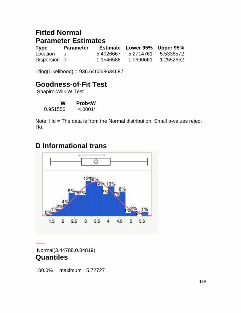
169

Fitted Normal Parameter Estimates Type Parameter Estimate Lower 95% Upper 95% Location μ 5.4026667 5.2714761 5.5338572 Dispersion σ 1.1546588 1.0690661 1.2552652 -2log(Likelihood) = 936.646068634687

Goodness-of-Fit Test Shapiro-Wilk W Test

W Prob<W 0.951550 <.0001*

Note: Ho = The data is from the Normal distribution. Small p-values reject Ho.

D Informational trans

Normal(3.44788,0.84819)

Quantiles 100.0% maximum 5.72727

170

99.5% 5.68136 97.5% 5.09091 90.0% 4.54545 75.0% quartile 4.09091 50.0% median 3.45455 25.0% quartile 2.81818 10.0% 2.36364 2.5% 1.90909 0.5% 1.50045 0.0% minimum 1.45455

Summary Statistics Mean 3.4478788 Std Dev 0.8481943 Std Err Mean 0.0489705 Upper 95% Mean 3.5442493 Lower 95% Mean 3.3515082 N 300

Fitted Normal Parameter Estimates Type Parameter Estimate Lower 95% Upper 95% Location μ 3.4478788 3.3515082 3.5442493 Dispersion σ 0.8481943 0.7853192 0.9220982 -2log(Likelihood) = 751.57578911683

Goodness-of-Fit Test Shapiro-Wilk W Test

W Prob<W 0.992558 0.1397

Note: Ho = The data is from the Normal distribution. Small p-values reject Ho.

171

Oneway Analysis of A Personal involvement By Add

Oneway Anova Summary of Fit Rsquare 0.013706 Adj Rsquare 0.007064 Root Mean Square Error 1.200188 Mean of Response 5.226111 Observations (or Sum Wgts) 300

Analysis of Variance Source DF Sum of

Squares Mean Square F Ratio Prob > F

Add 2 5.94505 2.97252 2.0636 0.1288 Error 297 427.81431 1.44045 C. Total 299 433.75935

Means for Oneway Anova Level Number Mean Std Error Lower 95% Upper 95%

172

Level Number Mean Std Error Lower 95% Upper 95% BOTH 100 5.24917 0.12002 5.0130 5.4854 PADD 100 5.04333 0.12002 4.8071 5.2795 SAB 100 5.38583 0.12002 5.1496 5.6220 Std Error uses a pooled estimate of error variance

Wilcoxon / Kruskal-Wallis Tests (Rank Sums) Level Count Score Sum Expected

Score Score Mean (Mean-Mean0)/Std0

BOTH 100 14931.0 15050.0 149.310 -0.167 PADD 100 13796.5 15050.0 137.965 -1.770 SAB 100 16422.5 15050.0 164.225 1.938

1-way Test, ChiSquare Approximation ChiSquare DF Prob>ChiSq

4.6136 2 0.0996

Tests that the Variances are Equal

Level Count Std Dev MeanAbsDif

to Mean MeanAbsDif

to Median BOTH 100 1.107411 0.9026333 0.8941667 PADD 100 1.255766 0.9824667 0.9816667 SAB 100 1.232091 0.9772500 0.9641667 Test F Ratio DFNum DFDen Prob > F O'Brien[.5] 0.6431 2 297 0.5264 Brown-Forsythe 0.3866 2 297 0.6797 Levene 0.3839 2 297 0.6815 Bartlett 0.8823 2 . 0.4138

173

Welch's Test Welch Anova testing Means Equal, allowing Std Devs Not Equal

F Ratio DFNum DFDen Prob > F 1.9132 2 197.36 0.1503

Means Comparisons Comparisons for all pairs using Tukey-Kramer HSD Confidence Quantile

q* Alpha 2.35560 0.05

LSD Threshold Matrix Abs(Dif)-HSD SAB BOTH PADD SAB -0.39982 -0.26315 -0.05732 BOTH -0.26315 -0.39982 -0.19399 PADD -0.05732 -0.19399 -0.39982 Positive values show pairs of means that are significantly different.

Connecting Letters Report Level Mean SAB A 5.3858333 BOTH A 5.2491667 PADD A 5.0433333 Levels not connected by same letter are significantly different.

Level - Level Difference Std Err Dif Lower CL Upper CL p-Value SAB PADD 0.3425000 0.1697323 -0.057321 0.7423209 0.1097 BOTH PADD 0.2058333 0.1697323 -0.193988 0.6056542 0.4466 SAB BOTH 0.1366667 0.1697323 -0.263154 0.5364876 0.7001

174

Ordered Differences Report

Nonparametric Comparisons For Each Pair Using Wilcoxon Method

q* Alpha 1.95996 0.05

Level - Level Score Mean

Difference Std Err Dif Z p-Value Hodges-

Lehmann Lower CL Upper CL

SAB PADD 17.5100 8.182080 2.14004 0.0324* 0.333333 0.000000 0.6666667 SAB BOTH 9.9200 8.181549 1.21248 0.2253 0.166667 -0.083333 0.5000000 PADD BOTH -7.5400 8.182276 -0.92150 0.3568 -0.166667 -0.500000 0.1666667

Oneway Analysis of A Personal involvement By Q1

Oneway Anova Summary of Fit Rsquare 0.023649

175

Adj Rsquare 0.013753 Root Mean Square Error 1.196139 Mean of Response 5.226111 Observations (or Sum Wgts) 300

Analysis of Variance Source DF Sum of

Squares Mean Square F Ratio Prob > F

Q1 3 10.25788 3.41929 2.3899 0.0689 Error 296 423.50147 1.43075 C. Total 299 433.75935

Means for Oneway Anova Level Number Mean Std Error Lower 95% Upper 95% 1 22 5.35227 0.25502 4.8504 5.8542 2 186 5.32168 0.08771 5.1491 5.4943 3 19 4.61404 0.27441 4.0740 5.1541 4 73 5.10388 0.14000 4.8284 5.3794 Std Error uses a pooled estimate of error variance

Wilcoxon / Kruskal-Wallis Tests (Rank Sums) Level Count Score Sum Expected

Score Score Mean (Mean-Mean0)/Std0

1 22 3382.00 3311.00 153.727 0.180 2 186 29552.5 27993.0 158.884 2.138 3 19 1967.50 2859.50 103.553 -2.437 4 73 10248.0 10986.5 140.384 -1.145

1-way Test, ChiSquare Approximation ChiSquare DF Prob>ChiSq

8.3320 3 0.0396*

176

Tests that the Variances are Equal

Level Count Std Dev MeanAbsDif

to Mean MeanAbsDif

to Median 1 22 0.941030 0.838843 0.8068182 2 186 1.239314 1.009818 0.9937276 3 19 1.180543 0.859187 0.8464912 4 73 1.152759 0.859354 0.8424658 Test F Ratio DFNum DFDen Prob > F O'Brien[.5] 0.5847 3 296 0.6255 Brown-Forsythe 0.9840 3 296 0.4006 Levene 1.1109 3 296 0.3449 Bartlett 0.9037 3 . 0.4384

Welch's Test Welch Anova testing Means Equal, allowing Std Devs Not Equal

F Ratio DFNum DFDen Prob > F 2.4154 3 52.822 0.0767

Means Comparisons Comparisons for all pairs using Tukey-Kramer HSD Confidence Quantile

q* Alpha 2.58371 0.05

177

LSD Threshold Matrix Abs(Dif)-HSD 1 2 4 3 1 -0.9318 -0.6662 -0.5033 -0.2297 2 -0.6662 -0.3205 -0.2090 -0.0367 4 -0.5033 -0.2090 -0.5115 -0.3061 3 -0.2297 -0.0367 -0.3061 -1.0027 Positive values show pairs of means that are significantly different.

Connecting Letters Report Level Mean 1 A 5.3522727 2 A 5.3216846 4 A 5.1038813 3 A 4.6140351 Levels not connected by same letter are significantly different.

Ordered Differences Report

Nonparametric Comparisons For Each Pair Using Wilcoxon Method

q* Alpha 1.95996 0.05

Level - Level Score Mean

Difference Std Err Dif Z p-Value Hodges-

Lehmann Lower CL Upper CL

4 3 12.1053 6.87220 1.76148 0.0782 0.416667 -0.08333 1.00000 2 1 3.0499 13.56463 0.22484 0.8221 0.083333 -0.41667 0.58333

Level - Level Difference Std Err Dif Lower CL Upper CL p-Value 1 3 0.7382376 0.3746152 -0.229660 1.706135 0.2015 2 3 0.7076495 0.2880881 -0.036687 1.451986 0.0691 4 3 0.4898462 0.3080614 -0.306096 1.285788 0.3858 1 4 0.2483914 0.2909180 -0.503257 1.000040 0.8285 2 4 0.2178033 0.1652013 -0.209029 0.644636 0.5519 1 2 0.0305881 0.2696780 -0.666182 0.727358 0.9995

178

Level - Level Score Mean Difference

Std Err Dif Z p-Value Hodges-Lehmann

Lower CL Upper CL

4 1 -3.3717 6.70010 -0.50324 0.6148 -0.166667 -0.66667 0.41667 3 1 -7.2093 3.74746 -1.92379 0.0544 -0.541667 -1.33333 0.00000 4 2 -16.4712 10.34192 -1.59267 0.1112 -0.250000 -0.58333 0.08333 3 2 -36.8060 14.28251 -2.57700 0.0100* -0.750000 -1.25000 -0.16667

Oneway Analysis of A Personal involvement By Q2

Oneway Anova Summary of Fit Rsquare 0.000598 Adj Rsquare -0.00276 Root Mean Square Error 1.206109 Mean of Response 5.226111 Observations (or Sum Wgts) 300

179

t Test 2-1 Assuming equal variances Difference -0.05962 t Ratio -0.4221 Std Err Dif 0.14125 DF 298 Upper CL Dif 0.21834 Prob > |t| 0.6733 Lower CL Dif -0.33758 Prob > t 0.6634 Confidence 0.95 Prob < t 0.3366

Analysis of Variance Source DF Sum of

Squares Mean Square F Ratio Prob > F

Q2 1 0.25918 0.25918 0.1782 0.6733 Error 298 433.50017 1.45470 C. Total 299 433.75935

Means for Oneway Anova Level Number Mean Std Error Lower 95% Upper 95% 1 175 5.25095 0.09117 5.0715 5.4304 2 125 5.19133 0.10788 4.9790 5.4036 Std Error uses a pooled estimate of error variance

Wilcoxon / Kruskal-Wallis Tests (Rank Sums) Level Count Score Sum Expected

Score Score Mean (Mean-Mean0)/Std0

1 175 26591.0 26337.5 151.949 0.342 2 125 18559.0 18812.5 148.472 -0.342

180

2-Sample Test, Normal Approximation S Z Prob>|Z|

18559 -0.34167 0.7326

1-way Test, ChiSquare Approximation ChiSquare DF Prob>ChiSq

0.1172 1 0.7321

Tests that the Variances are Equal

Level Count Std Dev MeanAbsDif

to Mean MeanAbsDif

to Median 1 175 1.195991 0.9609034 0.9566667 2 125 1.220165 0.9621013 0.9540000 Test F Ratio DFNum DFDen p-Value O'Brien[.5] 0.0447 1 298 0.8328 Brown-Forsythe 0.0009 1 298 0.9755 Levene 0.0002 1 298 0.9887 Bartlett 0.0579 1 . 0.8098 F Test 2-sided 1.0408 124 174 0.8026

Welch's Test Welch Anova testing Means Equal, allowing Std Devs Not Equal

F Ratio DFNum DFDen Prob > F 0.1770 1 263.99 0.6743

t Test

0.4207

181

Means Comparisons Comparisons for all pairs using Tukey-Kramer HSD Confidence Quantile

q* Alpha 1.96796 0.05

LSD Threshold Matrix Abs(Dif)-HSD 1 2 1 -0.25375 -0.21835 2 -0.21835 -0.30024 Positive values show pairs of means that are significantly different.

Nonparametric Comparisons For Each Pair Using Wilcoxon Method

q* Alpha 1.95996 0.05

Level - Level Score Mean

Difference Std Err Dif Z p-Value Hodges-

Lehmann Lower CL Upper CL

2 1 -3.46971 10.15504 -0.341674 0.7326 -0.083333 -0.333333 0.2500000

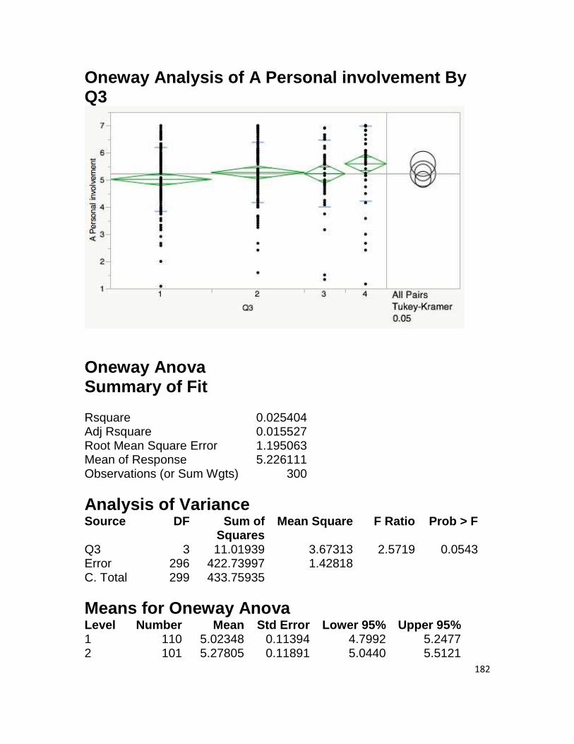
182

Oneway Analysis of A Personal involvement By Q3

Oneway Anova Summary of Fit Rsquare 0.025404 Adj Rsquare 0.015527 Root Mean Square Error 1.195063 Mean of Response 5.226111 Observations (or Sum Wgts) 300

Analysis of Variance Source DF Sum of

Squares Mean Square F Ratio Prob > F

Q3 3 11.01939 3.67313 2.5719 0.0543 Error 296 422.73997 1.42818 C. Total 299 433.75935

Means for Oneway Anova Level Number Mean Std Error Lower 95% Upper 95% 1 110 5.02348 0.11394 4.7992 5.2477 2 101 5.27805 0.11891 5.0440 5.5121

183

Level Number Mean Std Error Lower 95% Upper 95% 3 44 5.23295 0.18016 4.8784 5.5875 4 45 5.59815 0.17815 5.2475 5.9487 Std Error uses a pooled estimate of error variance

Wilcoxon / Kruskal-Wallis Tests (Rank Sums) Level Count Score Sum Expected

Score Score Mean (Mean-Mean0)/Std0

1 110 14710.5 16555.0 133.732 -2.548 2 101 15455.5 15200.5 153.025 0.359 3 44 6670.50 6622.00 151.602 0.090 4 45 8313.50 6772.50 184.744 2.872

1-way Test, ChiSquare Approximation ChiSquare DF Prob>ChiSq

11.2237 3 0.0106*

Tests that the Variances are Equal

Level Count Std Dev MeanAbsDif

to Mean MeanAbsDif

to Median 1 110 1.179275 0.960275 0.9598485 2 101 1.110698 0.891890 0.8869637 3 44 1.226271 0.904959 0.8958333 4 45 1.374517 1.022963 0.9944444 Test F Ratio DFNum DFDen Prob > F O'Brien[.5] 0.7562 3 296 0.5195 Brown-Forsythe 0.3069 3 296 0.8204 Levene 0.4014 3 296 0.7521

184

Test F Ratio DFNum DFDen Prob > F Bartlett 0.9974 3 . 0.3928

Welch's Test Welch Anova testing Means Equal, allowing Std Devs Not Equal

F Ratio DFNum DFDen Prob > F 2.2188 3 116.98 0.0896

Means Comparisons Comparisons for all pairs using Tukey-Kramer HSD Confidence Quantile

q* Alpha 2.58371 0.05

LSD Threshold Matrix Abs(Dif)-HSD 4 2 3 1 4 -0.65094 -0.23331 -0.28944 0.02828 2 -0.23331 -0.43450 -0.51264 -0.17095 3 -0.28944 -0.51264 -0.65830 -0.34130 1 0.02828 -0.17095 -0.34130 -0.41635 Positive values show pairs of means that are significantly different.

Connecting Letters Report Level Mean 4 A 5.5981481 2 A B 5.2780528 3 A B 5.2329545 1 B 5.0234848 Levels not connected by same letter are significantly different.

Level - Level Difference Std Err Dif Lower CL Upper CL p-Value 4 1 0.5746633 0.2114726 0.028279 1.121047 0.0349*

185

Ordered Differences Report

Nonparametric Comparisons For Each Pair Using Wilcoxon Method

q* Alpha 1.95996 0.05

Level - Level Score Mean

Difference Std Err Dif Z p-Value Hodges-

Lehmann Lower CL Upper CL

4 1 25.1444 7.939610 3.16696 0.0015* 0.6666667 0.250000 1.083333 4 2 15.7243 7.574266 2.07602 0.0379* 0.4166667 0.000000 0.833333 2 1 13.5792 8.411008 1.61446 0.1064 0.2500000 -0.083333 0.583333 4 3 11.1025 5.471320 2.02922 0.0424* 0.4166667 0.000000 0.916667 3 1 10.3409 7.952155 1.30039 0.1935 0.2500000 -0.166667 0.666667 3 2 -0.9462 7.583574 -0.12477 0.9007 0.0000000 -0.416667 0.416667

4 3 0.3651936 0.2533688 -0.289438 1.019826 0.4746 4 2 0.3200953 0.2141905 -0.233311 0.873502 0.4421 2 1 0.2545680 0.1646929 -0.170951 0.680087 0.4116 3 1 0.2094697 0.2131712 -0.341303 0.760242 0.7595 2 3 0.0450983 0.2158678 -0.512642 0.602838 0.9968

186

Oneway Analysis of A Personal involvement By Q4

Oneway Anova Summary of Fit Rsquare 0.026048 Adj Rsquare 0.016177 Root Mean Square Error 1.194669 Mean of Response 5.226111 Observations (or Sum Wgts) 300

Analysis of Variance Source DF Sum of

Squares Mean Square F Ratio Prob > F

Q4 3 11.29841 3.76614 2.6388 0.0498* Error 296 422.46094 1.42723 C. Total 299 433.75935

Means for Oneway Anova Level Number Mean Std Error Lower 95% Upper 95% 1 228 5.16886 0.07912 5.0132 5.3246

187

Level Number Mean Std Error Lower 95% Upper 95% 2 60 5.45556 0.15423 5.1520 5.7591 3 2 3.41667 0.84476 1.7542 5.0792 4 10 5.51667 0.37779 4.7732 6.2602 Std Error uses a pooled estimate of error variance

Wilcoxon / Kruskal-Wallis Tests (Rank Sums) Level Count Score Sum Expected

Score Score Mean (Mean-Mean0)/Std0

1 228 33223.5 34314.0 145.717 -1.699 2 60 10197.5 9030.00 169.958 1.942 3 2 63.000 301.000 31.500 -1.943 4 10 1666.00 1505.00 166.600 0.595

1-way Test, ChiSquare Approximation ChiSquare DF Prob>ChiSq

7.8260 3 0.0497*

Tests that the Variances are Equal

Level Count Std Dev MeanAbsDif

to Mean MeanAbsDif

to Median 1 228 1.183483 0.9530432 0.9466374 2 60 1.266740 0.9711111 0.9555556 3 2 1.060660 0.7500000 0.7500000 4 10 0.984290 0.7300000 0.7166667 Test F Ratio DFNum DFDen Prob > F O'Brien[.5] 0.3671 2 295 0.6931 Brown-Forsythe 0.3572 3 296 0.7840

188

Test F Ratio DFNum DFDen Prob > F Levene 0.3831 3 296 0.7653 Bartlett 0.3208 3 . 0.8103 Warning: Small sample sizes. Use Caution.

Welch's Test Welch Anova testing Means Equal, allowing Std Devs Not Equal

F Ratio DFNum DFDen Prob > F 2.3706 3 4.5636 0.1966

Means Comparisons Comparisons for all pairs using Tukey-Kramer HSD Confidence Quantile

q* Alpha 2.58371 0.05

LSD Threshold Matrix Abs(Dif)-HSD 4 2 1 3 4 -1.3804 -0.9932 -0.6495 -0.2909 2 -0.9932 -0.5635 -0.1612 -0.1798 1 -0.6495 -0.1612 -0.2891 -0.4400 3 -0.2909 -0.1798 -0.4400 -3.0867 Positive values show pairs of means that are significantly different.

Connecting Letters Report Level Mean 4 A 5.5166667 2 A 5.4555556 1 A 5.1688596 3 A 3.4166667 Levels not connected by same letter are significantly different.

189

Ordered Differences Report Level - Level Difference Std Err Dif Lower CL Upper CL p-Value 4 3 2.100000 0.9253863 -0.290931 4.490931 0.1076 2 3 2.038889 0.8587221 -0.179801 4.257579 0.0843 1 3 1.752193 0.8484552 -0.439970 3.944356 0.1670 4 1 0.347807 0.3859833 -0.649462 1.345076 0.8043 2 1 0.286696 0.1733407 -0.161167 0.734558 0.3501 4 2 0.061111 0.4080570 -0.993190 1.115413 0.9988

Nonparametric Comparisons For Each Pair Using Wilcoxon Method

q* Alpha 1.95996 0.05

Level - Level Score Mean Difference

Std Err Dif Z p-Value Hodges-Lehmann

Lower CL Upper CL

2 1 23.2737 12.07960 1.92669 0.0540 0.33333 0.00000 0.666667 4 1 17.0671 22.23613 0.76754 0.4428 0.25000 -0.41667 1.000000 4 3 5.1000 2.79285 1.82609 0.0678 2.08333 . . 4 2 -1.3417 6.94331 -0.19323 0.8468 -0.08333 -0.83333 0.750000 3 2 -25.3167 12.95467 -1.95425 0.0507 -2.25000 -4.16667 0.083333 3 1 -90.2851 47.24009 -1.91120 0.0560 -1.83333 -3.58333 0.083333

190

Oneway Analysis of A Personal involvement By Q5

Oneway Anova Summary of Fit Rsquare 0.026243 Adj Rsquare 0.016374 Root Mean Square Error 1.194548 Mean of Response 5.226111 Observations (or Sum Wgts) 300

Analysis of Variance Source DF Sum of

Squares Mean Square F Ratio Prob > F

Q5 3 11.38332 3.79444 2.6591 0.0484* Error 296 422.37603 1.42695 C. Total 299 433.75935

Means for Oneway Anova Level Number Mean Std Error Lower 95% Upper 95%

191

Level Number Mean Std Error Lower 95% Upper 95% 1 10 4.42500 0.37775 3.6816 5.1684 2 85 5.14118 0.12957 4.8862 5.3962 3 176 5.24953 0.09004 5.0723 5.4267 4 29 5.60920 0.22182 5.1726 6.0457 Std Error uses a pooled estimate of error variance

Wilcoxon / Kruskal-Wallis Tests (Rank Sums) Level Count Score Sum Expected

Score Score Mean (Mean-Mean0)/Std0

1 10 986.500 1505.00 98.650 -1.921 2 85 11932.5 12792.5 140.382 -1.270 3 176 27126.0 26488.0 154.125 0.862 4 29 5105.00 4364.50 176.034 1.667

1-way Test, ChiSquare Approximation ChiSquare DF Prob>ChiSq

7.5545 3 0.0562

Tests that the Variances are Equal

Level Count Std Dev MeanAbsDif

to Mean MeanAbsDif

to Median 1 10 1.509972 1.021667 0.958333 2 85 1.067499 0.863645 0.859804 3 176 1.267434 1.019483 1.004261 4 29 0.945201 0.739398 0.738506 Test F Ratio DFNum DFDen Prob > F O'Brien[.5] 1.7712 3 296 0.1527

192

Test F Ratio DFNum DFDen Prob > F Brown-Forsythe 1.3918 3 296 0.2454 Levene 1.8581 3 296 0.1367 Bartlett 2.3105 3 . 0.0741

Welch's Test Welch Anova testing Means Equal, allowing Std Devs Not Equal

F Ratio DFNum DFDen Prob > F 2.5892 3 35.864 0.0680

Means Comparisons Comparisons for all pairs using Tukey-Kramer HSD Confidence Quantile

q* Alpha 2.58371 0.05

LSD Threshold Matrix Abs(Dif)-HSD 4 3 2 1 4 -0.8105 -0.2589 -0.1957 0.0524 3 -0.2589 -0.3290 -0.2993 -0.1788 2 -0.1957 -0.2993 -0.4734 -0.3156 1 0.0524 -0.1788 -0.3156 -1.3803 Positive values show pairs of means that are significantly different.

Connecting Letters Report Level Mean 4 A 5.6091954 3 A B 5.2495265 2 A B 5.1411765 1 B 4.4250000 Levels not connected by same letter are significantly different.

Level - Level Difference Std Err Dif Lower CL Upper CL p-Value

193

Ordered Differences Report

Nonparametric Comparisons For Each Pair Using Wilcoxon Method

q* Alpha 1.95996 0.05

Level - Level Score Mean

Difference Std Err Dif Z p-Value Hodges-

Lehmann Lower CL Upper CL

3 1 32.12727 17.49532 1.836335 0.0663 0.875000 -0.083333 1.666667 2 1 14.64118 9.21110 1.589515 0.1119 0.666667 -0.166667 1.416667 4 2 14.38296 7.10381 2.024682 0.0429* 0.500000 0.000000 0.916667 4 3 13.89694 11.88402 1.169381 0.2423 0.250000 -0.166667 0.750000 3 2 11.85491 9.96726 1.189386 0.2343 0.166667 -0.083333 0.500000 4 1 11.02759 4.17637 2.640472 0.0083* 1.083333 0.333333 1.916667

4 1 1.184195 0.4380635 0.052366 2.316025 0.0363* 3 1 0.824527 0.3883327 -0.178813 1.827866 0.1481 2 1 0.716176 0.3993522 -0.315634 1.747987 0.2786 4 2 0.468019 0.2568903 -0.195712 1.131749 0.2651 4 3 0.359669 0.2394007 -0.258873 0.978211 0.4374 3 2 0.108350 0.1577823 -0.299314 0.516014 0.9021

194

Oneway Analysis of A Personal involvement By Q6

Oneway Anova Summary of Fit Rsquare 0.000576 Adj Rsquare -0.00278 Root Mean Square Error 1.206122 Mean of Response 5.226111 Observations (or Sum Wgts) 300

t Test 2-1 Assuming equal variances Difference -0.06189 t Ratio -0.41457 Std Err Dif 0.14928 DF 298 Upper CL Dif 0.23189 Prob > |t| 0.6788

195

Lower CL Dif -0.35566 Prob > t 0.6606 Confidence 0.95 Prob < t 0.3394

Analysis of Variance Source DF Sum of

Squares Mean Square F Ratio Prob > F

Q6 1 0.25002 0.25002 0.1719 0.6788 Error 298 433.50933 1.45473 C. Total 299 433.75935

Means for Oneway Anova Level Number Mean Std Error Lower 95% Upper 95% 1 204 5.24592 0.08445 5.0797 5.4121 2 96 5.18403 0.12310 4.9418 5.4263 Std Error uses a pooled estimate of error variance

Wilcoxon / Kruskal-Wallis Tests (Rank Sums) Level Count Score Sum Expected

Score Score Mean (Mean-Mean0)/Std0

1 204 31132.0 30702.0 152.608 0.613 2 96 14018.0 14448.0 146.021 -0.613

2-Sample Test, Normal Approximation S Z Prob>|Z|

14018 -0.61302 0.5399

1-way Test, ChiSquare Approximation ChiSquare DF Prob>ChiSq

0.3767 1 0.5394

196

Tests that the Variances are Equal

Level Count Std Dev MeanAbsDif

to Mean MeanAbsDif

to Median 1 204 1.215598 0.9499872 0.9444444 2 96 1.185618 0.9805411 0.9791667 Test F Ratio DFNum DFDen p-Value O'Brien[.5] 0.0603 1 298 0.8062 Brown-Forsythe 0.1446 1 298 0.7040 Levene 0.1156 1 298 0.7341 Bartlett 0.0799 1 . 0.7774 F Test 2-sided 1.0512 203 95 0.7937

Welch's Test Welch Anova testing Means Equal, allowing Std Devs Not Equal

F Ratio DFNum DFDen Prob > F 0.1750 1 190.43 0.6762

t Test

0.4183

Means Comparisons Comparisons for all pairs using Tukey-Kramer HSD Confidence Quantile

q* Alpha 1.96796 0.05

197

LSD Threshold Matrix Abs(Dif)-HSD 1 2 1 -0.23502 -0.23189 2 -0.23189 -0.34260 Positive values show pairs of means that are significantly different.

Nonparametric Comparisons For Each Pair Using Wilcoxon Method

Level - Level Score Mean Difference

Std Err Dif Z p-Value Hodges-Lehmann

Lower CL Upper CL

2 1 -6.57935 10.73260 -0.613025 0.5399 -0.083333 -0.333333 0.1666667

q* Alpha 1.95996 0.05

198

Oneway Analysis of B Trustworthiness By Add

Oneway Anova Summary of Fit Rsquare 0.005726 Adj Rsquare -0.00097 Root Mean Square Error 1.212159 Mean of Response 5.307333 Observations (or Sum Wgts) 300

Analysis of Variance Source DF Sum of

Squares Mean Square F Ratio Prob > F

Add 2 2.51307 1.25653 0.8552 0.4263 Error 297 436.39080 1.46933 C. Total 299 438.90387

Means for Oneway Anova Level Number Mean Std Error Lower 95% Upper 95% BOTH 100 5.18200 0.12122 4.9434 5.4206 PADD 100 5.34200 0.12122 5.1034 5.5806 SAB 100 5.39800 0.12122 5.1594 5.6366

199

Std Error uses a pooled estimate of error variance

Wilcoxon / Kruskal-Wallis Tests (Rank Sums) Level Count Score Sum Expected

Score Score Mean (Mean-Mean0)/Std0

BOTH 100 13973.5 15050.0 139.735 -1.523 PADD 100 14890.0 15050.0 148.900 -0.226 SAB 100 16286.5 15050.0 162.865 1.750

1-way Test, ChiSquare Approximation ChiSquare DF Prob>ChiSq

3.6250 2 0.1632

Tests that the Variances are Equal

Level Count Std Dev MeanAbsDif

to Mean MeanAbsDif

to Median BOTH 100 1.172787 0.936520 0.922000 PADD 100 1.045353 0.878640 0.874000 SAB 100 1.392765 1.082400 1.078000 Test F Ratio DFNum DFDen Prob > F O'Brien[.5] 3.2729 2 297 0.0393 Brown-Forsythe 1.9861 2 297 0.1390 Levene 2.1218 2 297 0.1216 Bartlett 4.1571 2 . 0.0157

Welch's Test Welch Anova testing Means Equal, allowing Std Devs Not Equal

200

F Ratio DFNum DFDen Prob > F 0.8314 2 195.48 0.4370

Means Comparisons Comparisons for all pairs using Tukey-Kramer HSD Confidence Quantile

q* Alpha 2.35560 0.05

LSD Threshold Matrix Abs(Dif)-HSD SAB PADD BOTH SAB -0.40381 -0.34781 -0.18781 PADD -0.34781 -0.40381 -0.24381 BOTH -0.18781 -0.24381 -0.40381 Positive values show pairs of means that are significantly different.

Connecting Letters Report Level Mean SAB A 5.3980000 PADD A 5.3420000 BOTH A 5.1820000 Levels not connected by same letter are significantly different.

Ordered Differences Report

Nonparametric Comparisons For Each Pair Using Wilcoxon Method

q* Alpha

Level - Level Difference Std Err Dif Lower CL Upper CL p-Value SAB BOTH 0.2160000 0.1714252 -0.187809 0.6198087 0.4190 PADD BOTH 0.1600000 0.1714252 -0.243809 0.5638087 0.6196 SAB PADD 0.0560000 0.1714252 -0.347809 0.4598087 0.9429

201

q* Alpha 1.95996 0.05

Oneway Analysis of B Trustworthiness By Q1

Oneway Anova Summary of Fit Rsquare 0.019858 Adj Rsquare 0.009924 Root Mean Square Error 1.205545 Mean of Response 5.307333

Level - Level Score Mean Difference

Std Err Dif Z p-Value Hodges-Lehmann

Lower CL Upper CL

SAB BOTH 14.89000 8.160768 1.824583 0.0681 0.4000000 0.000000 0.6000000 SAB PADD 9.82000 8.161920 1.203148 0.2289 0.2000000 -0.200000 0.6000000 PADD BOTH 6.62000 8.162178 0.811058 0.4173 0.2000000 -0.200000 0.4000000

202

Observations (or Sum Wgts) 300

Analysis of Variance Source DF Sum of

Squares Mean Square F Ratio Prob > F

Q1 3 8.71559 2.90520 1.9990 0.1142 Error 296 430.18828 1.45334 C. Total 299 438.90387

Means for Oneway Anova Level Number Mean Std Error Lower 95% Upper 95% 1 22 5.86364 0.25702 5.3578 6.3695 2 186 5.21398 0.08839 5.0400 5.3879 3 19 5.35789 0.27657 4.8136 5.9022 4 73 5.36438 0.14110 5.0867 5.6421 Std Error uses a pooled estimate of error variance

Wilcoxon / Kruskal-Wallis Tests (Rank Sums) Level Count Score Sum Expected

Score Score Mean (Mean-Mean0)/Std0

1 22 4192.00 3311.00 190.545 2.254 2 186 26623.5 27993.0 143.137 -1.882 3 19 2905.00 2859.50 152.895 0.123 4 73 11429.5 10986.5 156.568 0.688

1-way Test, ChiSquare Approximation ChiSquare DF Prob>ChiSq

6.4342 3 0.0923

203

Tests that the Variances are Equal

Level Count Std Dev MeanAbsDif

to Mean MeanAbsDif

to Median 1 22 0.869343 0.694215 0.6818182 2 186 1.235169 1.004475 0.9924731 3 19 1.148098 0.991690 0.9894737 4 73 1.226713 0.912216 0.9068493 Test F Ratio DFNum DFDen Prob > F O'Brien[.5] 0.7369 3 296 0.5307 Brown-Forsythe 1.2448 3 296 0.2936 Levene 1.3634 3 296 0.2541 Bartlett 1.3163 3 . 0.2670

Welch's Test Welch Anova testing Means Equal, allowing Std Devs Not Equal

F Ratio DFNum DFDen Prob > F 3.2341 3 53.666 0.0293*

Means Comparisons Comparisons for all pairs using Tukey-Kramer HSD Confidence Quantile

q* Alpha 2.58371 0.05

204

LSD Threshold Matrix Abs(Dif)-HSD 1 4 3 2 1 -0.9391 -0.2583 -0.4698 -0.0526 4 -0.2583 -0.5156 -0.7957 -0.2798 3 -0.4698 -0.7957 -1.0106 -0.6063 2 -0.0526 -0.2798 -0.6063 -0.3230 Positive values show pairs of means that are significantly different.

Connecting Letters Report Level Mean 1 A 5.8636364 4 A 5.3643836 3 A 5.3578947 2 A 5.2139785 Levels not connected by same letter are significantly different.

Ordered Differences Report

Nonparametric Comparisons For Each Pair Using Wilcoxon Method

q* Alpha 1.95996 0.05

Level - Level Score Mean

Difference Std Err Dif Z p-Value Hodges-

Lehmann Lower CL Upper CL

4 2 11.7502 10.31982 1.13860 0.2549 0.200000 -0.20000 0.4000000

Level - Level Difference Std Err Dif Lower CL Upper CL p-Value 1 2 0.6496579 0.2717986 -0.052591 1.351907 0.0812 1 3 0.5057416 0.3775611 -0.469767 1.481250 0.5385 1 4 0.4992528 0.2932057 -0.258306 1.256812 0.3241 4 2 0.1504051 0.1665004 -0.279784 0.580594 0.8031 3 2 0.1439162 0.2903535 -0.606273 0.894106 0.9600 4 3 0.0064888 0.3104839 -0.795712 0.808690 1.0000

205

Level - Level Score Mean Difference

Std Err Dif Z p-Value Hodges-Lehmann

Lower CL Upper CL

3 2 6.5549 14.25391 0.45987 0.6456 0.200000 -0.60000 0.6000000 4 3 1.1608 6.85178 0.16941 0.8655 0.000000 -0.60000 0.6000000 3 1 -4.8553 3.73370 -1.30039 0.1935 -0.400000 -1.20000 0.2000000 4 1 -11.2983 6.67778 -1.69192 0.0907 -0.400000 -1.00000 0.0000000 2 1 -32.4809 13.53539 -2.39971 0.0164* -0.600000 -1.00000 0.0000000

Oneway Analysis of B Trustworthiness By Q2

Oneway Anova Summary of Fit Rsquare 0.014332 Adj Rsquare 0.011024 Root Mean Square Error 1.204875 Mean of Response 5.307333 Observations (or Sum Wgts) 300

206

t Test 2-1 Assuming equal variances Difference -0.29371 t Ratio -2.0816 Std Err Dif 0.14110 DF 298 Upper CL Dif -0.01603 Prob > |t| 0.0382* Lower CL Dif -0.57139 Prob > t 0.9809 Confidence 0.95 Prob < t 0.0191*

Analysis of Variance Source DF Sum of

Squares Mean Square F Ratio Prob > F

Q2 1 6.29038 6.29038 4.3330 0.0382* Error 298 432.61349 1.45172 C. Total 299 438.90387

Means for Oneway Anova Level Number Mean Std Error Lower 95% Upper 95% 1 175 5.42971 0.09108 5.2505 5.6090 2 125 5.13600 0.10777 4.9239 5.3481 Std Error uses a pooled estimate of error variance

Wilcoxon / Kruskal-Wallis Tests (Rank Sums) Level Count Score Sum Expected

Score Score Mean (Mean-Mean0)/Std0

1 175 27710.5 26337.5 158.346 1.858 2 125 17439.5 18812.5 139.516 -1.858

207

2-Sample Test, Normal Approximation S Z Prob>|Z|

17439.5 -1.85780 0.0632

1-way Test, ChiSquare Approximation ChiSquare DF Prob>ChiSq

3.4539 1 0.0631

Tests that the Variances are Equal

Level Count Std Dev MeanAbsDif

to Mean MeanAbsDif

to Median 1 175 1.131182 0.896418 0.885714 2 125 1.301265 1.055232 1.044800 Test F Ratio DFNum DFDen p-Value O'Brien[.5] 2.3136 1 298 0.1293 Brown-Forsythe 3.1850 1 298 0.0753 Levene 3.5867 1 298 0.0592 Bartlett 2.8669 1 . 0.0904 F Test 2-sided 1.3233 124 174 0.0886

Welch's Test Welch Anova testing Means Equal, allowing Std Devs Not Equal

F Ratio DFNum DFDen Prob > F 4.1359 1 243.44 0.0431*

t Test

2.0337

208

Means Comparisons Comparisons for all pairs using Tukey-Kramer HSD Confidence Quantile

q* Alpha 1.96796 0.05

LSD Threshold Matrix Abs(Dif)-HSD 1 2 1 -0.25349 0.01603 2 0.01603 -0.29993 Positive values show pairs of means that are significantly different.

Nonparametric Comparisons For Each Pair Using Wilcoxon Method

q* Alpha 1.95996 0.05

Level - Level Score Mean

Difference Std Err Dif Z p-Value Hodges-

Lehmann Lower CL Upper CL

2 1 -18.8229 10.13179 -1.85780 0.0632 -0.200000 -0.600000 0

209

Oneway Analysis of B Trustworthiness By Q3

Oneway Anova Summary of Fit Rsquare 0.004777 Adj Rsquare -0.00531 Root Mean Square Error 1.214784 Mean of Response 5.307333 Observations (or Sum Wgts) 300

Analysis of Variance Source DF Sum of

Squares Mean Square F Ratio Prob > F

Q3 3 2.09669 0.69890 0.4736 0.7009 Error 296 436.80718 1.47570 C. Total 299 438.90387

Means for Oneway Anova Level Number Mean Std Error Lower 95% Upper 95% 1 110 5.32182 0.11583 5.0939 5.5498 2 101 5.23168 0.12088 4.9938 5.4696 3 44 5.26364 0.18314 4.9032 5.6240 4 45 5.48444 0.18109 5.1281 5.8408

210

Std Error uses a pooled estimate of error variance

Wilcoxon / Kruskal-Wallis Tests (Rank Sums) Level Count Score Sum Expected

Score Score Mean (Mean-Mean0)/Std0

1 110 16352.5 16555.0 148.659 -0.280 2 101 14620.0 15200.5 144.752 -0.819 3 44 6427.50 6622.00 146.080 -0.366 4 45 7750.00 6772.50 172.222 1.826

1-way Test, ChiSquare Approximation ChiSquare DF Prob>ChiSq

3.4472 3 0.3277

Tests that the Variances are Equal

Level Count Std Dev MeanAbsDif

to Mean MeanAbsDif

to Median 1 110 1.069029 0.867107 0.860000 2 101 1.200577 0.979355 0.964356 3 44 1.231956 0.978926 0.972727 4 45 1.528808 1.164642 1.120000 Test F Ratio DFNum DFDen Prob > F O'Brien[.5] 2.5530 3 296 0.0557 Brown-Forsythe 1.2267 3 296 0.3001 Levene 1.8428 3 296 0.1394 Bartlett 2.9055 3 . 0.0333

211

Welch's Test Welch Anova testing Means Equal, allowing Std Devs Not Equal

F Ratio DFNum DFDen Prob > F 0.3513 3 114.8 0.7883

Means Comparisons Comparisons for all pairs using Tukey-Kramer HSD Confidence Quantile

q* Alpha 2.58371 0.05

LSD Threshold Matrix Abs(Dif)-HSD 4 1 3 2 4 -0.66169 -0.39277 -0.44463 -0.30978 1 -0.39277 -0.42322 -0.50168 -0.34241 3 -0.44463 -0.50168 -0.66916 -0.53499 2 -0.30978 -0.34241 -0.53499 -0.44167 Positive values show pairs of means that are significantly different.

Connecting Letters Report Level Mean 4 A 5.4844444 1 A 5.3218182 3 A 5.2636364 2 A 5.2316832 Levels not connected by same letter are significantly different.

Level - Level Difference Std Err Dif Lower CL Upper CL p-Value 4 2 0.2527613 0.2177251 -0.309778 0.8153001 0.6520 4 3 0.2208081 0.2575499 -0.444627 0.8862428 0.8267 4 1 0.1626263 0.2149623 -0.392774 0.7180268 0.8738 1 2 0.0901350 0.1674107 -0.342406 0.5226760 0.9496

212

Ordered Differences Report

Nonparametric Comparisons For Each Pair Using Wilcoxon Method

q* Alpha 1.95996 0.05

Level - Level Score Mean

Difference Std Err Dif Z p-Value Hodges-

Lehmann Lower CL Upper CL

4 2 12.9135 7.555348 1.70919 0.0874 0.4000000 0.000000 0.800000 4 1 12.8227 7.914357 1.62019 0.1052 0.4000000 0.000000 0.800000 4 3 7.3942 5.445821 1.35777 0.1745 0.4000000 -0.200000 1.000000 3 2 0.5221 7.570850 0.06896 0.9450 0.0000000 -0.400000 0.400000 3 1 -1.4477 7.935315 -0.18244 0.8552 0.0000000 -0.400000 0.400000 2 1 -3.0577 8.394856 -0.36423 0.7157 0.0000000 -0.400000 0.200000

Oneway Analysis of B Trustworthiness By Q4

1 3 0.0581818 0.2166889 -0.501680 0.6180435 0.9932 3 2 0.0319532 0.2194300 -0.534991 0.5988970 0.9989

213

Oneway Anova Summary of Fit Rsquare 0.018568 Adj Rsquare 0.008621 Root Mean Square Error 1.206338 Mean of Response 5.307333 Observations (or Sum Wgts) 300

Analysis of Variance Source DF Sum of

Squares Mean Square F Ratio Prob > F

Q4 3 8.14941 2.71647 1.8667 0.1353 Error 296 430.75446 1.45525 C. Total 299 438.90387

Means for Oneway Anova Level Number Mean Std Error Lower 95% Upper 95% 1 228 5.29123 0.07989 5.1340 5.4485 2 60 5.42000 0.15574 5.1135 5.7265 3 2 3.40000 0.85301 1.7213 5.0787 4 10 5.38000 0.38148 4.6292 6.1308 Std Error uses a pooled estimate of error variance

Wilcoxon / Kruskal-Wallis Tests (Rank Sums) Level Count Score Sum Expected

Score Score Mean (Mean-Mean0)/Std0

1 228 33996.0 34314.0 149.105 -0.496 2 60 9622.00 9030.00 160.367 0.987 3 2 42.500 301.000 21.250 -2.116 4 10 1489.50 1505.00 148.950 -0.056

1-way Test, ChiSquare Approximation ChiSquare DF Prob>ChiSq

5.3065 3 0.1507

214

Tests that the Variances are Equal

Level Count Std Dev MeanAbsDif

to Mean MeanAbsDif

to Median 1 228 1.194743 0.947645 0.933333 2 60 1.274894 1.033333 1.033333 3 2 0.565685 0.400000 0.400000 4 10 1.080946 0.896000 0.860000 Test F Ratio DFNum DFDen Prob > F O'Brien[.5] 0.2390 2 295 0.7875 Brown-Forsythe 0.6637 3 296 0.5750 Levene 0.6588 3 296 0.5780 Bartlett 0.4006 3 . 0.7526 Warning: Small sample sizes. Use Caution.

Welch's Test Welch Anova testing Means Equal, allowing Std Devs Not Equal

F Ratio DFNum DFDen Prob > F 5.9422 3 4.7354 0.0457*

Means Comparisons Comparisons for all pairs using Tukey-Kramer HSD Confidence Quantile

q* Alpha 2.58371 0.05

215

LSD Threshold Matrix Abs(Dif)-HSD 2 4 1 3 2 -0.5691 -1.0246 -0.3235 -0.2204 4 -1.0246 -1.3939 -0.9182 -0.4343 1 -0.3235 -0.9182 -0.2919 -0.3223 3 -0.2204 -0.4343 -0.3223 -3.1168 Positive values show pairs of means that are significantly different.

Connecting Letters Report Level Mean 2 A 5.4200000 4 A 5.3800000 1 A 5.2912281 3 A 3.4000000 Levels not connected by same letter are significantly different.

Ordered Differences Report

Nonparametric Comparisons For Each Pair Using Wilcoxon Method

q* Alpha 1.95996 0.05

Level - Level Score Mean

Difference Std Err Dif Z p-Value Hodges-

Lehmann Lower CL Upper CL

2 1 10.9368 12.05226 0.90745 0.3642 0.20000 -0.20000 0.400000

Level - Level Difference Std Err Dif Lower CL Upper CL p-Value 2 3 2.020000 0.8671101 -0.22036 4.260362 0.0937 4 3 1.980000 0.9344255 -0.43429 4.394286 0.1494 1 3 1.891228 0.8567429 -0.32235 4.104805 0.1236 2 1 0.128772 0.1750339 -0.32347 0.581009 0.8826 4 1 0.088772 0.3897536 -0.91824 1.095783 0.9958 2 4 0.040000 0.4120429 -1.02460 1.104600 0.9997

216

Level - Level Score Mean Difference

Std Err Dif Z p-Value Hodges-Lehmann

Lower CL Upper CL

4 3 5.4000 2.75846 1.95762 0.0503 1.80000 . . 4 1 -0.4697 22.18967 -0.02117 0.9831 0.00000 -0.80000 0.800000 4 2 -2.2750 6.91415 -0.32904 0.7421 0.00000 -1.00000 0.600000 3 2 -26.6083 12.90997 -2.06107 0.0393* -2.20000 -3.80000 -0.200000 3 1 -99.1118 47.14756 -2.10216 0.0355* -2.00000 -3.20000 -0.200000

Oneway Analysis of B Trustworthiness By Q5

Oneway Anova Summary of Fit Rsquare 0.035184 Adj Rsquare 0.025405 Root Mean Square Error 1.196083 Mean of Response 5.307333 Observations (or Sum Wgts) 300

217

Analysis of Variance Source DF Sum of

Squares Mean Square F Ratio Prob > F

Q5 3 15.44228 5.14743 3.5981 0.0140* Error 296 423.46159 1.43061 C. Total 299 438.90387

Means for Oneway Anova Level Number Mean Std Error Lower 95% Upper 95% 1 10 5.28000 0.37823 4.5356 6.0244 2 85 5.63529 0.12973 5.3800 5.8906 3 176 5.21818 0.09016 5.0407 5.3956 4 29 4.89655 0.22211 4.4594 5.3337 Std Error uses a pooled estimate of error variance

Wilcoxon / Kruskal-Wallis Tests (Rank Sums) Level Count Score Sum Expected

Score Score Mean (Mean-Mean0)/Std0

1 10 1489.50 1505.00 148.950 -0.056 2 85 14701.5 12792.5 172.959 2.826 3 176 25376.0 26488.0 144.182 -1.506 4 29 3583.00 4364.50 123.552 -1.764

1-way Test, ChiSquare Approximation ChiSquare DF Prob>ChiSq

9.4833 3 0.0235*

Tests that the Variances are Equal

218

Level Count Std Dev MeanAbsDif to Mean

MeanAbsDif to Median

1 10 1.494285 1.240000 1.240000 2 85 1.032416 0.856747 0.847059 3 176 1.218200 0.961983 0.945455 4 29 1.390396 1.113912 1.110345 Test F Ratio DFNum DFDen Prob > F O'Brien[.5] 1.6572 3 296 0.1763 Brown-Forsythe 1.5035 3 296 0.2137 Levene 1.5947 3 296 0.1907 Bartlett 1.9228 3 . 0.1234

Welch's Test Welch Anova testing Means Equal, allowing Std Devs Not Equal

F Ratio DFNum DFDen Prob > F 3.7427 3 34.838 0.0197*

Means Comparisons Comparisons for all pairs using Tukey-Kramer HSD Confidence Quantile

q* Alpha 2.58371 0.05

LSD Threshold Matrix Abs(Dif)-HSD 2 1 3 4 2 -0.4740 -0.6778 0.0089 0.0742 1 -0.6778 -1.3820 -0.9428 -0.7498 3 0.0089 -0.9428 -0.3294 -0.2977 4 0.0742 -0.7498 -0.2977 -0.8116 Positive values show pairs of means that are significantly different.

Connecting Letters Report Level Mean

219

Level Mean 2 A 5.6352941 1 A B 5.2800000 3 B 5.2181818 4 B 4.8965517 Levels not connected by same letter are significantly different.

Ordered Differences Report

Nonparametric Comparisons For Each Pair Using Wilcoxon Method

q* Alpha 1.95996 0.05

Level - Level Score Mean

Difference Std Err Dif Z p-Value Hodges-

Lehmann Lower CL Upper CL

2 1 6.3147 9.17375 0.68835 0.4912 0.200000 -0.60000 1.20000 3 1 -2.1665 17.45815 -0.12410 0.9012 0.000000 -1.00000 1.00000 4 1 -2.6897 4.16789 -0.64533 0.5187 -0.400000 -1.60000 0.80000 4 3 -14.9412 11.85924 -1.25988 0.2077 -0.400000 -0.80000 0.20000 4 2 -17.9440 7.08181 -2.53382 0.0113* -0.800000 -1.20000 -0.20000 3 2 -25.5243 9.94363 -2.56690 0.0103* -0.400000 -0.60000 0.00000

Level - Level Difference Std Err Dif Lower CL Upper CL p-Value 2 4 0.7387424 0.2572202 0.074160 1.403325 0.0226* 2 3 0.4171123 0.1579849 0.008925 0.825300 0.0431* 1 4 0.3834483 0.4386261 -0.749835 1.516732 0.8182 2 1 0.3552941 0.3998651 -0.677842 1.388430 0.8108 3 4 0.3216301 0.2397081 -0.297707 0.940967 0.5371 1 3 0.0618182 0.3888314 -0.942810 1.066446 0.9986

220

Oneway Analysis of B Trustworthiness By Q6

Oneway Anova Summary of Fit Rsquare 0.001136 Adj Rsquare -0.00222 Root Mean Square Error 1.212914 Mean of Response 5.307333 Observations (or Sum Wgts) 300

t Test 2-1 Assuming equal variances Difference -0.08738 t Ratio -0.58205 Std Err Dif 0.15012 DF 298 Upper CL Dif 0.20805 Prob > |t| 0.5610

221

Lower CL Dif -0.38281 Prob > t 0.7195 Confidence 0.95 Prob < t 0.2805

Analysis of Variance Source DF Sum of

Squares Mean Square F Ratio Prob > F

Q6 1 0.49840 0.49840 0.3388 0.5610 Error 298 438.40547 1.47116 C. Total 299 438.90387

Means for Oneway Anova Level Number Mean Std Error Lower 95% Upper 95% 1 204 5.33529 0.08492 5.1682 5.5024 2 96 5.24792 0.12379 5.0043 5.4915 Std Error uses a pooled estimate of error variance

Wilcoxon / Kruskal-Wallis Tests (Rank Sums) Level Count Score Sum Expected

Score Score Mean (Mean-Mean0)/Std0

1 204 31047.0 30702.0 152.191 0.493 2 96 14103.0 14448.0 146.906 -0.493

2-Sample Test, Normal Approximation S Z Prob>|Z|

14103 -0.49283 0.6221

1-way Test, ChiSquare Approximation ChiSquare DF Prob>ChiSq

0.2436 1 0.6216

222

Tests that the Variances are Equal

Level Count Std Dev MeanAbsDif

to Mean MeanAbsDif

to Median 1 204 1.189995 0.949423 0.9411765 2 96 1.260491 1.010590 0.9979167 Test F Ratio DFNum DFDen p-Value O'Brien[.5] 0.3460 1 298 0.5569 Brown-Forsythe 0.3687 1 298 0.5442 Levene 0.4651 1 298 0.4958 Bartlett 0.4328 1 . 0.5106 F Test 2-sided 1.1220 95 203 0.4970

Welch's Test Welch Anova testing Means Equal, allowing Std Devs Not Equal

F Ratio DFNum DFDen Prob > F 0.3250 1 176.84 0.5693

t Test

0.5701

Means Comparisons Comparisons for all pairs using Tukey-Kramer HSD Confidence Quantile

q* Alpha 1.96796 0.05

223

LSD Threshold Matrix Abs(Dif)-HSD 1 2 1 -0.23634 -0.20805 2 -0.20805 -0.34453 Positive values show pairs of means that are significantly different.

Nonparametric Comparisons For Each Pair Using Wilcoxon Method

q* Alpha 1.95996 0.05

Level - Level Score Mean

Difference Std Err Dif Z p-Value Hodges-

Lehmann Lower CL Upper CL

2 1 -5.27727 10.70803 -0.492833 0.6221 0 -0.400000 0.2000000

224

Oneway Analysis of C Expertise By Add

Oneway Anova Summary of Fit Rsquare 0.031267 Adj Rsquare 0.024744 Root Mean Square Error 1.140284 Mean of Response 5.402667 Observations (or Sum Wgts) 300

Analysis of Variance Source DF Sum of

Squares Mean Square F Ratio Prob > F

Add 2 12.46427 6.23213 4.7930 0.0089* Error 297 386.17360 1.30025 C. Total 299 398.63787

Means for Oneway Anova Level Number Mean Std Error Lower 95% Upper 95% BOTH 100 5.45800 0.11403 5.2336 5.6824

225

Level Number Mean Std Error Lower 95% Upper 95% PADD 100 5.13000 0.11403 4.9056 5.3544 SAB 100 5.62000 0.11403 5.3956 5.8444 Std Error uses a pooled estimate of error variance

Wilcoxon / Kruskal-Wallis Tests (Rank Sums) Level Count Score Sum Expected

Score Score Mean (Mean-Mean0)/Std0

BOTH 100 15451.0 15050.0 154.510 0.567 PADD 100 12854.5 15050.0 128.545 -3.109 SAB 100 16844.5 15050.0 168.445 2.541

1-way Test, ChiSquare Approximation ChiSquare DF Prob>ChiSq

10.9689 2 0.0042*

Tests that the Variances are Equal

Level Count Std Dev MeanAbsDif

to Mean MeanAbsDif

to Median BOTH 100 1.118547 0.8968400 0.8940000 PADD 100 1.152731 0.9220000 0.9220000 SAB 100 1.149264 0.9172000 0.8840000 Test F Ratio DFNum DFDen Prob > F O'Brien[.5] 0.0480 2 297 0.9531 Brown-Forsythe 0.0722 2 297 0.9304 Levene 0.0388 2 297 0.9620 Bartlett 0.0538 2 . 0.9476

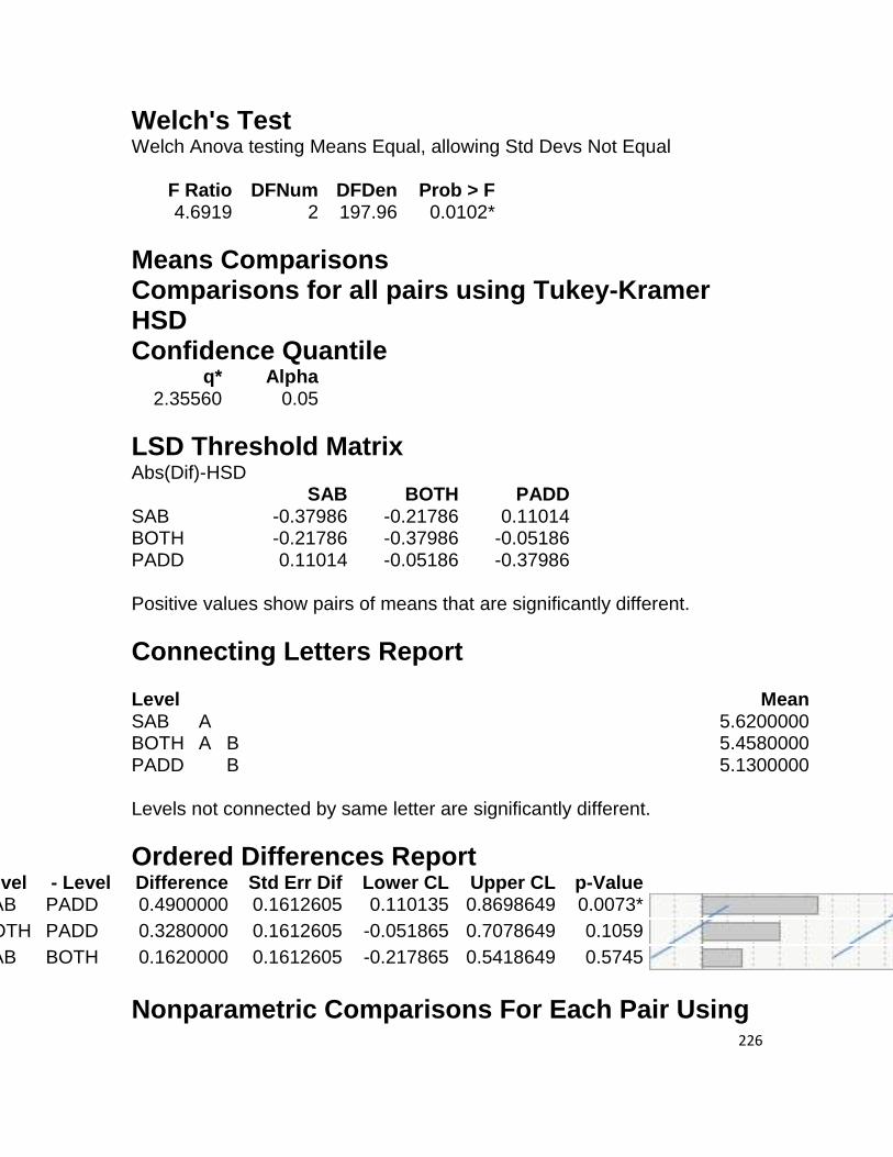
226

Welch's Test Welch Anova testing Means Equal, allowing Std Devs Not Equal

F Ratio DFNum DFDen Prob > F 4.6919 2 197.96 0.0102*

Means Comparisons Comparisons for all pairs using Tukey-Kramer HSD Confidence Quantile

q* Alpha 2.35560 0.05

LSD Threshold Matrix Abs(Dif)-HSD SAB BOTH PADD SAB -0.37986 -0.21786 0.11014 BOTH -0.21786 -0.37986 -0.05186 PADD 0.11014 -0.05186 -0.37986 Positive values show pairs of means that are significantly different.

Connecting Letters Report Level Mean SAB A 5.6200000 BOTH A B 5.4580000 PADD B 5.1300000 Levels not connected by same letter are significantly different.

Ordered Differences Report Level - Level Difference Std Err Dif Lower CL Upper CL p-Value SAB PADD 0.4900000 0.1612605 0.110135 0.8698649 0.0073* BOTH PADD 0.3280000 0.1612605 -0.051865 0.7078649 0.1059 SAB BOTH 0.1620000 0.1612605 -0.217865 0.5418649 0.5745

Nonparametric Comparisons For Each Pair Using

227

Wilcoxon Method q* Alpha

1.95996 0.05

Level - Level Score Mean Difference

Std Err Dif Z p-Value Hodges-Lehmann

Lower CL Upper CL

SAB PADD 26.4100 8.160199 3.23644 0.0012* 0.600000 0.200000 0.8000000 SAB BOTH 9.4600 8.150041 1.16073 0.2458 0.200000 0.000000 0.6000000 PADD BOTH -17.4800 8.162415 -2.14152 0.0322* -0.400000 -0.600000 0.0000000

Oneway Analysis of C Expertise By Q1

Oneway Anova Summary of Fit Rsquare 0.010287 Adj Rsquare 0.000256 Root Mean Square Error 1.154511 Mean of Response 5.402667 Observations (or Sum Wgts) 300

228

Analysis of Variance Source DF Sum of

Squares Mean Square F Ratio Prob > F

Q1 3 4.10088 1.36696 1.0256 0.3816 Error 296 394.53698 1.33290 C. Total 299 398.63787

Means for Oneway Anova Level Number Mean Std Error Lower 95% Upper 95% 1 22 5.48182 0.24614 4.9974 5.9662 2 186 5.45914 0.08465 5.2925 5.6257 3 19 5.00000 0.26486 4.4787 5.5213 4 73 5.33973 0.13513 5.0738 5.6057 Std Error uses a pooled estimate of error variance

Wilcoxon / Kruskal-Wallis Tests (Rank Sums) Level Count Score Sum Expected

Score Score Mean (Mean-Mean0)/Std0

1 22 3393.50 3311.00 154.250 0.210 2 186 28752.5 27993.0 154.583 1.044 3 19 2248.50 2859.50 118.342 -1.674 4 73 10755.5 10986.5 147.336 -0.359

1-way Test, ChiSquare Approximation ChiSquare DF Prob>ChiSq

3.1819 3 0.3644

Tests that the Variances are Equal

229

Level Count Std Dev MeanAbsDif to Mean

MeanAbsDif to Median

1 22 1.194685 0.9983471 0.9909091 2 186 1.137160 0.9213551 0.9107527 3 19 1.150845 0.9684211 0.9684211 4 73 1.187287 0.9312817 0.9123288 Test F Ratio DFNum DFDen Prob > F O'Brien[.5] 0.0783 3 296 0.9717 Brown-Forsythe 0.1157 3 296 0.9509 Levene 0.1057 3 296 0.9567 Bartlett 0.0821 3 . 0.9698

Welch's Test Welch Anova testing Means Equal, allowing Std Devs Not Equal

F Ratio DFNum DFDen Prob > F 1.0022 3 50.513 0.3995

Means Comparisons Comparisons for all pairs using Tukey-Kramer HSD Confidence Quantile

q* Alpha 2.58371 0.05

LSD Threshold Matrix Abs(Dif)-HSD 1 2 4 3 1 -0.89939 -0.64984 -0.58340 -0.45239 2 -0.64984 -0.30931 -0.29256 -0.25929 4 -0.58340 -0.29256 -0.49374 -0.42852 3 -0.45239 -0.25929 -0.42852 -0.96779 Positive values show pairs of means that are significantly different.

Connecting Letters Report Level Mean

230

Level Mean 1 A 5.4818182 2 A 5.4591398 4 A 5.3397260 3 A 5.0000000 Levels not connected by same letter are significantly different.

Ordered Differences Report

Nonparametric Comparisons For Each Pair Using Wilcoxon Method

q* Alpha 1.95996 0.05

Level - Level Score Mean

Difference Std Err Dif Z p-Value Hodges-

Lehmann Lower CL Upper CL

4 3 8.4239 6.85380 1.22909 0.2190 0.400000 -0.20000 1.000000 2 1 -0.3304 13.51812 -0.02444 0.9805 0.000000 -0.60000 0.600000 4 1 -1.7450 6.67773 -0.26132 0.7938 0.000000 -0.80000 0.400000 3 1 -4.4139 3.72959 -1.18347 0.2366 -0.600000 -1.20000 0.200000 4 2 -6.2566 10.31261 -0.60669 0.5441 0.000000 -0.40000 0.200000 3 2 -25.3785 14.23789 -1.78246 0.0747 -0.600000 -1.00000 0.000000

Level - Level Difference Std Err Dif Lower CL Upper CL p-Value 1 3 0.4818182 0.3615778 -0.452395 1.416031 0.5429 2 3 0.4591398 0.2780620 -0.259292 1.177572 0.3516 4 3 0.3397260 0.2973402 -0.428515 1.107967 0.6635 1 4 0.1420922 0.2807935 -0.583397 0.867582 0.9576 2 4 0.1194138 0.1594520 -0.292564 0.531392 0.8771 1 2 0.0226784 0.2602926 -0.649843 0.695199 0.9998

231

Oneway Analysis of C Expertise By Q2

Oneway Anova Summary of Fit Rsquare 9.786e-6 Adj Rsquare -0.00335 Root Mean Square Error 1.156589 Mean of Response 5.402667 Observations (or Sum Wgts) 300

t Test 2-1 Assuming equal variances Difference -0.00731 t Ratio -0.054 Std Err Dif 0.13545 DF 298 Upper CL Dif 0.25924 Prob > |t| 0.9570

232

Lower CL Dif -0.27387 Prob > t 0.5215 Confidence 0.95 Prob < t 0.4785

Analysis of Variance Source DF Sum of

Squares Mean Square F Ratio Prob > F

Q2 1 0.00390 0.00390 0.0029 0.9570 Error 298 398.63397 1.33770 C. Total 299 398.63787

Means for Oneway Anova Level Number Mean Std Error Lower 95% Upper 95% 1 175 5.40571 0.08743 5.2337 5.5778 2 125 5.39840 0.10345 5.1948 5.6020 Std Error uses a pooled estimate of error variance

Wilcoxon / Kruskal-Wallis Tests (Rank Sums) Level Count Score Sum Expected

Score Score Mean (Mean-Mean0)/Std0

1 175 26216.0 26337.5 149.806 -0.164 2 125 18934.0 18812.5 151.472 0.164

2-Sample Test, Normal Approximation S Z Prob>|Z|

18934 0.16388 0.8698

1-way Test, ChiSquare Approximation ChiSquare DF Prob>ChiSq

0.0271 1 0.8693

233

Tests that the Variances are Equal

Level Count Std Dev MeanAbsDif

to Mean MeanAbsDif

to Median 1 175 1.097212 0.890122 0.8845714 2 125 1.235104 1.000115 0.9920000 Test F Ratio DFNum DFDen p-Value O'Brien[.5] 2.0019 1 298 0.1582 Brown-Forsythe 1.6676 1 298 0.1976 Levene 1.9480 1 298 0.1638 Bartlett 2.0446 1 . 0.1527 F Test 2-sided 1.2671 124 174 0.1501

Welch's Test Welch Anova testing Means Equal, allowing Std Devs Not Equal

F Ratio DFNum DFDen Prob > F 0.0028 1 247.22 0.9578

t Test

0.0529

Means Comparisons Comparisons for all pairs using Tukey-Kramer HSD Confidence Quantile

q* Alpha 1.96796 0.05

234

LSD Threshold Matrix Abs(Dif)-HSD 1 2 1 -0.24333 -0.25924 2 -0.25924 -0.28791 Positive values show pairs of means that are significantly different.

Nonparametric Comparisons For Each Pair Using Wilcoxon Method

q* Alpha 1.95996 0.05

Oneway Analysis of C Expertise By Q3

Level - Level Score Mean Difference

Std Err Dif Z p-Value Hodges-Lehmann

Lower CL Upper CL

2 1 1.659429 10.12616 0.1638754 0.8698 0 -0.200000 0.2000000

235

Oneway Anova Summary of Fit Rsquare 0.013409 Adj Rsquare 0.00341 Root Mean Square Error 1.152689 Mean of Response 5.402667 Observations (or Sum Wgts) 300

Analysis of Variance Source DF Sum of

Squares Mean Square F Ratio Prob > F

Q3 3 5.34526 1.78175 1.3410 0.2612 Error 296 393.29261 1.32869 C. Total 299 398.63787

Means for Oneway Anova Level Number Mean Std Error Lower 95% Upper 95% 1 110 5.33818 0.10990 5.1219 5.5545 2 101 5.35248 0.11470 5.1268 5.5782 3 44 5.35455 0.17377 5.0126 5.6965 4 45 5.72000 0.17183 5.3818 6.0582 Std Error uses a pooled estimate of error variance

Wilcoxon / Kruskal-Wallis Tests (Rank Sums) Level Count Score Sum Expected

Score Score Mean (Mean-Mean0)/Std0

1 110 15787.5 16555.0 143.523 -1.063 2 101 14567.0 15200.5 144.228 -0.894 3 44 6633.00 6622.00 150.750 0.020 4 45 8162.50 6772.50 181.389 2.598

1-way Test, ChiSquare Approximation ChiSquare DF Prob>ChiSq

6.9905 3 0.0722

236

Tests that the Variances are Equal

Level Count Std Dev MeanAbsDif

to Mean MeanAbsDif

to Median 1 110 1.090659 0.892893 0.8872727 2 101 1.082275 0.875718 0.8752475 3 44 1.310327 1.001240 0.9545455 4 45 1.285160 1.027556 0.9555556 Test F Ratio DFNum DFDen Prob > F O'Brien[.5] 1.3156 3 296 0.2694 Brown-Forsythe 0.2121 3 296 0.8880 Levene 0.7855 3 296 0.5028 Bartlett 1.3469 3 . 0.2571

Welch's Test Welch Anova testing Means Equal, allowing Std Devs Not Equal

F Ratio DFNum DFDen Prob > F 1.1102 3 115.38 0.3480

Means Comparisons Comparisons for all pairs using Tukey-Kramer HSD Confidence Quantile

q* Alpha 2.58371 0.05

237

LSD Threshold Matrix Abs(Dif)-HSD 4 3 2 1 4 -0.62786 -0.26597 -0.16626 -0.14519 3 -0.26597 -0.63496 -0.53589 -0.51488 2 -0.16626 -0.53589 -0.41909 -0.39614 1 -0.14519 -0.51488 -0.39614 -0.40158 Positive values show pairs of means that are significantly different.

Connecting Letters Report Level Mean 4 A 5.7200000 3 A 5.3545455 2 A 5.3524752 1 A 5.3381818 Levels not connected by same letter are significantly different.

Ordered Differences Report

Nonparametric Comparisons For Each Pair Using Wilcoxon Method

q* Alpha 1.95996 0.05

Level - Level Score Mean

Difference Std Err Dif Z p-Value Hodges-

Lehmann Lower CL Upper CL

4 1 19.60202 7.919352 2.475205 0.0133* 0.6000000 0.000000 1.000000

Level - Level Difference Std Err Dif Lower CL Upper CL p-Value 4 1 0.3818182 0.2039742 -0.145192 0.9088287 0.2424 4 2 0.3675248 0.2065958 -0.166259 0.9013087 0.2855 4 3 0.3654545 0.2443849 -0.265966 0.9968747 0.4416 3 1 0.0163636 0.2056126 -0.514880 0.5476072 0.9998 2 1 0.0142934 0.1588533 -0.396138 0.4247245 0.9997 3 2 0.0020702 0.2082136 -0.535894 0.5400340 1.0000

238

Level - Level Score Mean Difference

Std Err Dif Z p-Value Hodges-Lehmann

Lower CL Upper CL

4 2 17.45897 7.551498 2.311987 0.0208* 0.6000000 0.000000 1.000000 4 3 9.84394 5.437349 1.810430 0.0702 0.4000000 0.000000 1.000000 3 1 3.97727 7.928229 0.501660 0.6159 0.0000000 -0.200000 0.400000 3 2 3.40965 7.558907 0.451078 0.6519 0.0000000 -0.200000 0.600000 2 1 0.28488 8.393240 0.033941 0.9729 0.0000000 -0.400000 0.200000

Oneway Analysis of C Expertise By Q4

Oneway Anova Summary of Fit Rsquare 0.022011 Adj Rsquare 0.012099 Root Mean Square Error 1.147652 Mean of Response 5.402667 Observations (or Sum Wgts) 300

239

Analysis of Variance Source DF Sum of

Squares Mean Square F Ratio Prob > F

Q4 3 8.77443 2.92481 2.2206 0.0858 Error 296 389.86344 1.31711 C. Total 299 398.63787

Means for Oneway Anova Level Number Mean Std Error Lower 95% Upper 95% 1 228 5.37632 0.07601 5.2267 5.5259 2 60 5.54333 0.14816 5.2518 5.8349 3 2 3.50000 0.81151 1.9029 5.0971 4 10 5.54000 0.36292 4.8258 6.2542 Std Error uses a pooled estimate of error variance

Wilcoxon / Kruskal-Wallis Tests (Rank Sums) Level Count Score Sum Expected

Score Score Mean (Mean-Mean0)/Std0

1 228 33479.5 34314.0 146.840 -1.304 2 60 9951.00 9030.00 165.850 1.537 3 2 53.500 301.000 26.750 -2.027 4 10 1666.00 1505.00 166.600 0.597

1-way Test, ChiSquare Approximation ChiSquare DF Prob>ChiSq

6.7424 3 0.0806

Tests that the Variances are Equal

240

Level Count Std Dev MeanAbsDif to Mean

MeanAbsDif to Median

1 228 1.111399 0.907802 0.9061404 2 60 1.249863 0.953667 0.8900000 3 2 0.707107 0.500000 0.5000000 4 10 1.366423 1.004000 0.9400000 Test F Ratio DFNum DFDen Prob > F O'Brien[.5] 0.9861 2 295 0.3743 Brown-Forsythe 0.2162 3 296 0.8851 Levene 0.3774 3 296 0.7694 Bartlett 0.6912 3 . 0.5573 Warning: Small sample sizes. Use Caution.

Welch's Test Welch Anova testing Means Equal, allowing Std Devs Not Equal

F Ratio DFNum DFDen Prob > F 3.9556 3 4.6129 0.0939

Means Comparisons Comparisons for all pairs using Tukey-Kramer HSD Confidence Quantile

q* Alpha 2.58371 0.05

LSD Threshold Matrix Abs(Dif)-HSD 2 4 1 3 2 -0.5414 -1.0095 -0.2632 -0.0880 4 -1.0095 -1.3261 -0.7943 -0.2568 1 -0.2632 -0.7943 -0.2777 -0.2296 3 -0.0880 -0.2568 -0.2296 -2.9652 Positive values show pairs of means that are significantly different.

241

Connecting Letters Report Level Mean 2 A 5.5433333 4 A 5.5400000 1 A 5.3763158 3 A 3.5000000 Levels not connected by same letter are significantly different.

Ordered Differences Report

Nonparametric Comparisons For Each Pair Using Wilcoxon Method

q* Alpha 1.95996 0.05

Level - Level Score Mean

Difference Std Err Dif Z p-Value Hodges-

Lehmann Lower CL Upper CL

2 1 18.3579 12.04581 1.52401 0.1275 0.20000 0.00000 0.600000 4 1 15.8145 22.17810 0.71307 0.4758 0.20000 -0.60000 1.000000 4 3 4.2000 2.77816 1.51179 0.1306 2.20000 . . 4 2 0.1167 6.90919 0.01689 0.9865 0.00000 -0.80000 0.800000 3 2 -25.5750 12.89947 -1.98264 0.0474* -2.20000 -3.60000 0.000000 3 1 -95.5811 47.12390 -2.02829 0.0425* -2.00000 -3.40000 0.000000

- Level Difference Std Err Dif Lower CL Upper CL p-Value 2 3 2.043333 0.8249272 -0.08804 4.174707 0.0656 4 3 2.040000 0.8889678 -0.25684 4.336836 0.1015 1 3 1.876316 0.8150643 -0.22958 3.982207 0.0999 2 1 0.167018 0.1665189 -0.26322 0.597254 0.7478 4 1 0.163684 0.3707929 -0.79434 1.121706 0.9712 2 4 0.003333 0.3919979 -1.00948 1.016143 1.0000

242

Oneway Analysis of C Expertise By Q5

Oneway Anova Summary of Fit Rsquare 0.02391 Adj Rsquare 0.014017 Root Mean Square Error 1.146538 Mean of Response 5.402667 Observations (or Sum Wgts) 300

Analysis of Variance Source DF Sum of

Squares Mean Square F Ratio Prob > F

Q5 3 9.53133 3.17711 2.4169 0.0665 Error 296 389.10653 1.31455 C. Total 299 398.63787

Means for Oneway Anova Level Number Mean Std Error Lower 95% Upper 95% 1 10 4.52000 0.36257 3.8065 5.2335 2 85 5.54353 0.12436 5.2988 5.7883

243

Level Number Mean Std Error Lower 95% Upper 95% 3 176 5.38523 0.08642 5.2151 5.5553 4 29 5.40000 0.21291 4.9810 5.8190 Std Error uses a pooled estimate of error variance

Wilcoxon / Kruskal-Wallis Tests (Rank Sums) Level Count Score Sum Expected

Score Score Mean (Mean-Mean0)/Std0

1 10 978.000 1505.00 97.800 -1.958 2 85 13456.5 12792.5 158.312 0.983 3 176 26426.5 26488.0 150.151 -0.083 4 29 4289.00 4364.50 147.897 -0.169

1-way Test, ChiSquare Approximation ChiSquare DF Prob>ChiSq

4.4374 3 0.2179

Tests that the Variances are Equal

Level Count Std Dev MeanAbsDif

to Mean MeanAbsDif

to Median 1 10 1.594992 1.320000 1.320000 2 85 1.059026 0.881993 0.880000 3 176 1.161481 0.925542 0.914773 4 29 1.132633 0.937931 0.917241 Test F Ratio DFNum DFDen Prob > F O'Brien[.5] 1.7023 3 296 0.1666 Brown-Forsythe 1.1863 3 296 0.3151 Levene 1.3130 3 296 0.2703

244

Test F Ratio DFNum DFDen Prob > F Bartlett 1.1618 3 . 0.3227

Welch's Test Welch Anova testing Means Equal, allowing Std Devs Not Equal

F Ratio DFNum DFDen Prob > F 1.4463 3 34.959 0.2460

Means Comparisons Comparisons for all pairs using Tukey-Kramer HSD Confidence Quantile

q* Alpha 2.58371 0.05

LSD Threshold Matrix Abs(Dif)-HSD 2 4 3 1 2 -0.4544 -0.4935 -0.2330 0.0332 4 -0.4935 -0.7779 -0.5789 -0.2063 3 -0.2330 -0.5789 -0.3158 -0.0978 1 0.0332 -0.2063 -0.0978 -1.3248 Positive values show pairs of means that are significantly different.

Connecting Letters Report Level Mean 2 A 5.5435294 4 A B 5.4000000 3 A B 5.3852273 1 B 4.5200000 Levels not connected by same letter are significantly different.

Ordered Differences Report - Level Difference Std Err Dif Lower CL Upper CL p-Value 1 1.023529 0.3833017 0.033188 2.013870 0.0397*

245

- Level Difference Std Err Dif Lower CL Upper CL p-Value 1 0.880000 0.4204571 -0.206340 1.966340 0.1578 1 0.865227 0.3727250 -0.097787 1.828241 0.0955 3 0.158302 0.1514408 -0.232977 0.549581 0.7229 4 0.143529 0.2465655 -0.493525 0.780584 0.9374 3 0.014773 0.2297788 -0.578909 0.608455 0.9999

Nonparametric Comparisons For Each Pair Using Wilcoxon Method

q* Alpha 1.95996 0.05

Level - Level Score Mean

Difference Std Err Dif Z p-Value Hodges-

Lehmann Lower CL Upper CL

3 1 32.2858 17.43459 1.85182 0.0641 1.00000 0.000000 2.000000 2 1 19.1676 9.18689 2.08641 0.0369* 1.20000 0.000000 2.200000 4 1 6.5224 4.16874 1.56460 0.1177 1.00000 -0.200000 2.200000 4 3 -1.8074 11.84525 -0.15258 0.8787 0.00000 -0.400000 0.400000 4 2 -3.6304 7.08486 -0.51242 0.6084 -0.20000 -0.600000 0.400000 3 2 -7.1967 9.93655 -0.72426 0.4689 0.00000 -0.400000 0.200000

246

Oneway Analysis of C Expertise By Q6

Oneway Anova Summary of Fit Rsquare 2.816e-5 Adj Rsquare -0.00333 Root Mean Square Error 1.156578 Mean of Response 5.402667 Observations (or Sum Wgts) 300

t Test 2-1 Assuming equal variances Difference -0.01311 t Ratio -0.0916 Std Err Dif 0.14315 DF 298 Upper CL Dif 0.26860 Prob > |t| 0.9271

247

Lower CL Dif -0.29482 Prob > t 0.5365 Confidence 0.95 Prob < t 0.4635

Analysis of Variance Source DF Sum of

Squares Mean Square F Ratio Prob > F

Q6 1 0.01122 0.01122 0.0084 0.9271 Error 298 398.62664 1.33767 C. Total 299 398.63787

Means for Oneway Anova Level Number Mean Std Error Lower 95% Upper 95% 1 204 5.40686 0.08098 5.2475 5.5662 2 96 5.39375 0.11804 5.1614 5.6261 Std Error uses a pooled estimate of error variance

Wilcoxon / Kruskal-Wallis Tests (Rank Sums) Level Count Score Sum Expected

Score Score Mean (Mean-Mean0)/Std0

1 204 30516.5 30702.0 149.591 -0.265 2 96 14633.5 14448.0 152.432 0.265

2-Sample Test, Normal Approximation S Z Prob>|Z|

14633.5 0.26480 0.7912

1-way Test, ChiSquare Approximation ChiSquare DF Prob>ChiSq

0.0705 1 0.7906

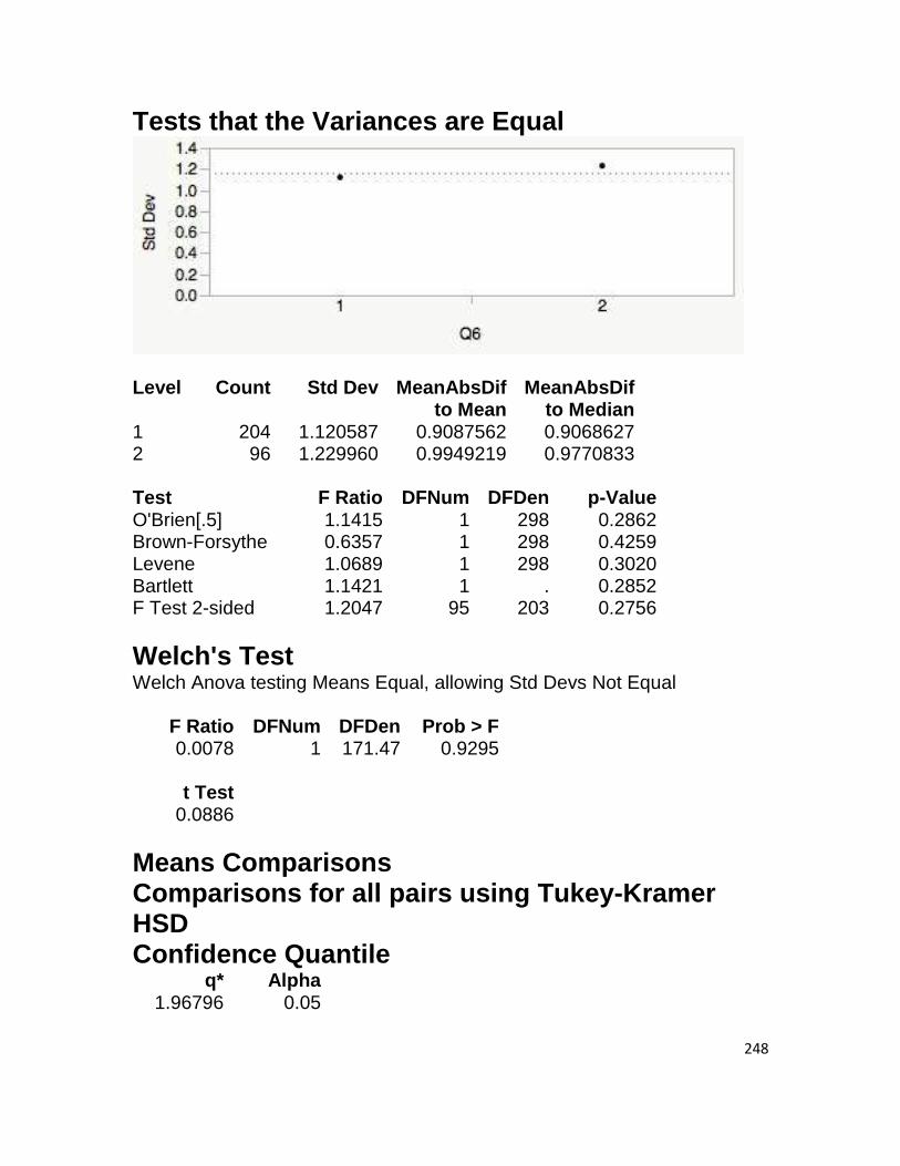
248

Tests that the Variances are Equal

Level Count Std Dev MeanAbsDif

to Mean MeanAbsDif

to Median 1 204 1.120587 0.9087562 0.9068627 2 96 1.229960 0.9949219 0.9770833 Test F Ratio DFNum DFDen p-Value O'Brien[.5] 1.1415 1 298 0.2862 Brown-Forsythe 0.6357 1 298 0.4259 Levene 1.0689 1 298 0.3020 Bartlett 1.1421 1 . 0.2852 F Test 2-sided 1.2047 95 203 0.2756

Welch's Test Welch Anova testing Means Equal, allowing Std Devs Not Equal

F Ratio DFNum DFDen Prob > F 0.0078 1 171.47 0.9295

t Test

0.0886

Means Comparisons Comparisons for all pairs using Tukey-Kramer HSD Confidence Quantile

q* Alpha 1.96796 0.05

249

LSD Threshold Matrix Abs(Dif)-HSD 1 2 1 -0.22537 -0.26860 2 -0.26860 -0.32853 Positive values show pairs of means that are significantly different.

Nonparametric Comparisons For Each Pair Using Wilcoxon Method

q* Alpha 1.95996 0.05

Level - Level Score Mean Difference

Std Err Dif Z p-Value Hodges-Lehmann

Lower CL Upper CL

2 1 2.833946 10.70208 0.2648034 0.7912 0 -0.200000 0.4000000

250

Oneway Analysis of D Informational trans By Add

Oneway Anova Summary of Fit Rsquare 0.028788 Adj Rsquare 0.022248 Root Mean Square Error 0.838706 Mean of Response 3.447879 Observations (or Sum Wgts) 300

Analysis of Variance Source DF Sum of

Squares Mean Square F Ratio Prob > F

Add 2 6.19262 3.09631 4.4017 0.0131* Error 297 208.91802 0.70343 C. Total 299 215.11063

Means for Oneway Anova Level Number Mean Std Error Lower 95% Upper 95% BOTH 100 3.64000 0.08387 3.4749 3.8051

251

Level Number Mean Std Error Lower 95% Upper 95% PADD 100 3.40909 0.08387 3.2440 3.5741 SAB 100 3.29455 0.08387 3.1295 3.4596 Std Error uses a pooled estimate of error variance

Wilcoxon / Kruskal-Wallis Tests (Rank Sums) Level Count Score Sum Expected

Score Score Mean (Mean-Mean0)/Std0

BOTH 100 16972.5 15050.0 169.725 2.715 PADD 100 14524.0 15050.0 145.240 -0.742 SAB 100 13653.5 15050.0 136.535 -1.972

1-way Test, ChiSquare Approximation ChiSquare DF Prob>ChiSq

7.8815 2 0.0194*

Tests that the Variances are Equal

Level Count Std Dev MeanAbsDif

to Mean MeanAbsDif

to Median BOTH 100 0.8305785 0.6674909 0.6672727 PADD 100 0.8217451 0.6636364 0.6636364 SAB 100 0.8632250 0.7218182 0.7218182 Test F Ratio DFNum DFDen Prob > F O'Brien[.5] 0.1754 2 297 0.8392 Brown-Forsythe 0.4619 2 297 0.6306 Levene 0.4609 2 297 0.6312 Bartlett 0.1333 2 . 0.8752

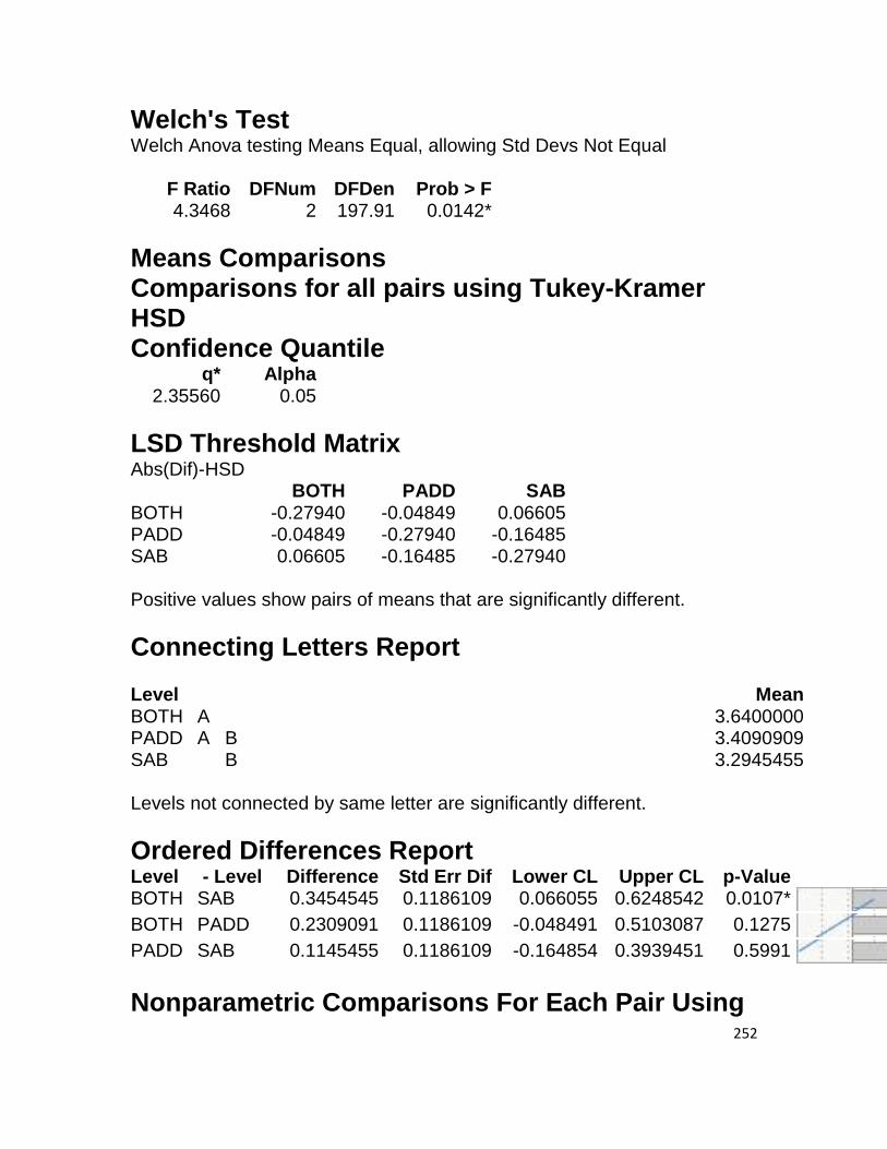
252

Welch's Test Welch Anova testing Means Equal, allowing Std Devs Not Equal

F Ratio DFNum DFDen Prob > F 4.3468 2 197.91 0.0142*

Means Comparisons Comparisons for all pairs using Tukey-Kramer HSD Confidence Quantile

q* Alpha 2.35560 0.05

LSD Threshold Matrix Abs(Dif)-HSD BOTH PADD SAB BOTH -0.27940 -0.04849 0.06605 PADD -0.04849 -0.27940 -0.16485 SAB 0.06605 -0.16485 -0.27940 Positive values show pairs of means that are significantly different.

Connecting Letters Report Level Mean BOTH A 3.6400000 PADD A B 3.4090909 SAB B 3.2945455 Levels not connected by same letter are significantly different.

Ordered Differences Report Level - Level Difference Std Err Dif Lower CL Upper CL p-Value BOTH SAB 0.3454545 0.1186109 0.066055 0.6248542 0.0107* BOTH PADD 0.2309091 0.1186109 -0.048491 0.5103087 0.1275 PADD SAB 0.1145455 0.1186109 -0.164854 0.3939451 0.5991

Nonparametric Comparisons For Each Pair Using

253

Wilcoxon Method q* Alpha

1.95996 0.05

Level - Level Score Mean Difference

Std Err Dif Z p-Value Hodges-Lehmann

Lower CL Upper CL

SAB PADD -6.1900 8.179712 -0.75675 0.4492 -0.090909 -0.363636 0.181818 PADD BOTH -16.7100 8.179030 -2.04303 0.0410* -0.272727 -0.454545 0.000000 SAB BOTH -21.7200 8.179740 -2.65534 0.0079* -0.363636 -0.636364 -0.090909

Oneway Analysis of D Informational trans By Q1

Oneway Anova Summary of Fit Rsquare 0.019299 Adj Rsquare 0.00936 Root Mean Square Error 0.844216 Mean of Response 3.447879 Observations (or Sum Wgts) 300

254

Analysis of Variance Source DF Sum of

Squares Mean Square F Ratio Prob > F

Q1 3 4.15144 1.38381 1.9416 0.1229 Error 296 210.95919 0.71270 C. Total 299 215.11063

Means for Oneway Anova Level Number Mean Std Error Lower 95% Upper 95% 1 22 3.69835 0.17999 3.3441 4.0526 2 186 3.35924 0.06190 3.2374 3.4811 3 19 3.56938 0.19368 3.1882 3.9505 4 73 3.56663 0.09881 3.3722 3.7611 Std Error uses a pooled estimate of error variance

Wilcoxon / Kruskal-Wallis Tests (Rank Sums) Level Count Score Sum Expected

Score Score Mean (Mean-Mean0)/Std0

1 22 3951.50 3311.00 179.614 1.635 2 186 26191.0 27993.0 140.812 -2.472 3 19 2966.50 2859.50 156.132 0.291 4 73 12041.0 10986.5 164.945 1.636

1-way Test, ChiSquare Approximation ChiSquare DF Prob>ChiSq

6.9117 3 0.0748

Tests that the Variances are Equal

255

Level Count Std Dev MeanAbsDif to Mean

MeanAbsDif to Median

1 22 0.7715863 0.6322314 0.6322314 2 186 0.8466139 0.6964809 0.6964809 3 19 0.9441921 0.7096449 0.6794258 4 73 0.8317506 0.6640509 0.6637609 Test F Ratio DFNum DFDen Prob > F O'Brien[.5] 0.3672 3 296 0.7768 Brown-Forsythe 0.1622 3 296 0.9217 Levene 0.1818 3 296 0.9087 Bartlett 0.2768 3 . 0.8422

Welch's Test Welch Anova testing Means Equal, allowing Std Devs Not Equal

F Ratio DFNum DFDen Prob > F 1.9993 3 50.81 0.1258

Means Comparisons Comparisons for all pairs using Tukey-Kramer HSD Confidence Quantile

q* Alpha 2.58371 0.05

LSD Threshold Matrix Abs(Dif)-HSD 1 3 4 2 1 -0.65766 -0.55416 -0.39878 -0.15266 3 -0.55416 -0.70768 -0.55901 -0.31520 4 -0.39878 -0.55901 -0.36104 -0.09386 2 -0.15266 -0.31520 -0.09386 -0.22618 Positive values show pairs of means that are significantly different.

Connecting Letters Report Level Mean

256

Level Mean 1 A 3.6983471 3 A 3.5693780 4 A 3.5666252 2 A 3.3592375 Levels not connected by same letter are significantly different.

Ordered Differences Report Level - Level Difference Std Err Dif Lower CL Upper CL p-Value 1 2 0.3391096 0.1903344 -0.152660 0.8308787 0.2842 3 2 0.2101405 0.2033279 -0.315200 0.7354811 0.7299 4 2 0.2073876 0.1165965 -0.093864 0.5086392 0.2857 1 4 0.1317220 0.2053253 -0.398779 0.6622232 0.9184 1 3 0.1289691 0.2643974 -0.554157 0.8120957 0.9618 3 4 0.0027528 0.2174248 -0.559010 0.5645157 1.0000

Nonparametric Comparisons For Each Pair Using Wilcoxon Method

q* Alpha 1.95996 0.05

Level - Level Score Mean

Difference Std Err Dif Z p-Value Hodges-

Lehmann Lower CL Upper CL

4 2 20.6963 10.33949 2.00168 0.0453* 0.272727 0.000000 0.4545455 3 2 10.8765 14.27834 0.76175 0.4462 0.181818 -0.272727 0.6363636 4 3 3.2170 6.86737 0.46845 0.6395 0.090909 -0.363636 0.5454545 3 1 -3.0897 3.74501 -0.82502 0.4094 -0.181818 -0.818182 0.3636364 4 1 -4.7027 6.69836 -0.70206 0.4826 -0.181818 -0.545455 0.2727273 2 1 -26.8387 13.56116 -1.97909 0.0478* -0.363636 -0.727273 0.0000000

257

Oneway Analysis of D Informational trans By Q2

Oneway Anova Summary of Fit Rsquare 0.001172 Adj Rsquare -0.00218 Root Mean Square Error 0.849118 Mean of Response 3.447879 Observations (or Sum Wgts) 300

t Test 2-1 Assuming equal variances Difference 0.05881 t Ratio 0.591372 Std Err Dif 0.09944 DF 298 Upper CL Dif 0.25450 Prob > |t| 0.5547 Lower CL Dif -0.13689 Prob > t 0.2774 Confidence 0.95 Prob < t 0.7226

258

Analysis of Variance Source DF Sum of

Squares Mean Square F Ratio Prob > F

Q2 1 0.25215 0.252150 0.3497 0.5547 Error 298 214.85848 0.721002 C. Total 299 215.11063

Means for Oneway Anova Level Number Mean Std Error Lower 95% Upper 95% 1 175 3.42338 0.06419 3.2971 3.5497 2 125 3.48218 0.07595 3.3327 3.6316 Std Error uses a pooled estimate of error variance

Wilcoxon / Kruskal-Wallis Tests (Rank Sums) Level Count Score Sum Expected

Score Score Mean (Mean-Mean0)/Std0

1 175 25780.5 26337.5 147.317 -0.752 2 125 19369.5 18812.5 154.956 0.752

2-Sample Test, Normal Approximation S Z Prob>|Z|

19369.5 0.75178 0.4522

1-way Test, ChiSquare Approximation ChiSquare DF Prob>ChiSq

0.5662 1 0.4518

259

Tests that the Variances are Equal

Level Count Std Dev MeanAbsDif

to Mean MeanAbsDif

to Median 1 175 0.8415740 0.6789462 0.6779221 2 125 0.8595926 0.7053615 0.7018182 Test F Ratio DFNum DFDen p-Value O'Brien[.5] 0.0837 1 298 0.7726 Brown-Forsythe 0.1677 1 298 0.6825 Levene 0.2106 1 298 0.6466 Bartlett 0.0649 1 . 0.7989 F Test 2-sided 1.0433 124 174 0.7917

Welch's Test Welch Anova testing Means Equal, allowing Std Devs Not Equal

F Ratio DFNum DFDen Prob > F 0.3473 1 263.8 0.5562

t Test

0.5893

Means Comparisons Comparisons for all pairs using Tukey-Kramer HSD Confidence Quantile

q* Alpha 1.96796 0.05

260

LSD Threshold Matrix Abs(Dif)-HSD 2 1 2 -0.21137 -0.13689 1 -0.13689 -0.17864 Positive values show pairs of means that are significantly different.

Nonparametric Comparisons For Each Pair Using Wilcoxon Method

q* Alpha 1.95996 0.05

Level - Level Score Mean

Difference Std Err Dif Z p-Value Hodges-

Lehmann Lower CL Upper CL

2 1 7.632000 10.15192 0.7517789 0.4522 0.0909091 -0.090909 0.2727273

Oneway Analysis of D Informational trans By Q3

261

Oneway Anova Summary of Fit Rsquare 0.043313 Adj Rsquare 0.033617 Root Mean Square Error 0.833816 Mean of Response 3.447879 Observations (or Sum Wgts) 300

Analysis of Variance Source DF Sum of

Squares Mean Square F Ratio Prob > F

Q3 3 9.31702 3.10567 4.4670 0.0044* Error 296 205.79362 0.69525 C. Total 299 215.11063

Means for Oneway Anova Level Number Mean Std Error Lower 95% Upper 95% 1 110 3.57769 0.07950 3.4212 3.7341 2 101 3.53465 0.08297 3.3714 3.6979 3 44 3.28099 0.12570 3.0336 3.5284 4 45 3.09899 0.12430 2.8544 3.3436 Std Error uses a pooled estimate of error variance

Wilcoxon / Kruskal-Wallis Tests (Rank Sums) Level Count Score Sum Expected

Score Score Mean (Mean-Mean0)/Std0

1 110 18157.0 16555.0 165.064 2.213 2 101 16028.5 15200.5 158.698 1.166 3 44 5876.00 6622.00 133.545 -1.403 4 45 5088.50 6772.50 113.078 -3.140

1-way Test, ChiSquare Approximation ChiSquare DF Prob>ChiSq

14.0768 3 0.0028*

262

Tests that the Variances are Equal

Level Count Std Dev MeanAbsDif

to Mean MeanAbsDif

to Median 1 110 0.7970666 0.6498272 0.6487603 2 101 0.8241487 0.6413988 0.6408641 3 44 0.8561359 0.7197596 0.7148760 4 45 0.9183050 0.7160494 0.7111111 Test F Ratio DFNum DFDen Prob > F O'Brien[.5] 0.5838 3 296 0.6261 Brown-Forsythe 0.3785 3 296 0.7686 Levene 0.4518 3 296 0.7162 Bartlett 0.4612 3 . 0.7094

Welch's Test Welch Anova testing Means Equal, allowing Std Devs Not Equal

F Ratio DFNum DFDen Prob > F 3.9882 3 117.81 0.0096*

Means Comparisons Comparisons for all pairs using Tukey-Kramer HSD Confidence Quantile

q* Alpha 2.58371 0.05

263

LSD Threshold Matrix Abs(Dif)-HSD 1 2 3 4 1 -0.29049 -0.25386 -0.08759 0.09747 2 -0.25386 -0.30316 -0.13548 0.04954 3 -0.08759 -0.13548 -0.45931 -0.27475 4 0.09747 0.04954 -0.27475 -0.45417 Positive values show pairs of means that are significantly different.

Connecting Letters Report Level Mean 1 A 3.5776860 2 A 3.5346535 3 A B 3.2809917 4 B 3.0989899 Levels not connected by same letter are significantly different.

Ordered Differences Report Level - Level Difference Std Err Dif Lower CL Upper CL p-Value 1 4 0.4786961 0.1475480 0.097475 0.8599175 0.0071* 2 4 0.4356636 0.1494444 0.049542 0.8217847 0.0199* 1 3 0.2966942 0.1487331 -0.087589 0.6809778 0.1922 2 3 0.2536617 0.1506146 -0.135483 0.6428064 0.3339 3 4 0.1820018 0.1767797 -0.274746 0.6387497 0.7323 1 2 0.0430325 0.1149091 -0.253859 0.3399244 0.9821

Nonparametric Comparisons For Each Pair Using Wilcoxon Method

q* Alpha 1.95996 0.05

Level - Level Score Mean

Difference Std Err Dif Z p-Value Hodges-

Lehmann Lower CL Upper CL

2 1 -5.1278 8.407413 -0.60992 0.5419 -0.090909 -0.272727 0.181818 4 3 -5.9333 5.470993 -1.08451 0.2781 -0.181818 -0.545455 0.181818

264

Level - Level Score Mean Difference

Std Err Dif Z p-Value Hodges-Lehmann

Lower CL Upper CL

3 2 -12.1703 7.581049 -1.60536 0.1084 -0.272727 -0.636364 0.090909 3 1 -16.0523 7.949225 -2.01935 0.0435* -0.363636 -0.636364 0.000000 4 2 -23.2733 7.573433 -3.07301 0.0021* -0.545455 -0.818182 -0.181818 4 1 -25.8646 7.936651 -3.25889 0.0011* -0.545455 -0.909091 -0.272727

Oneway Analysis of D Informational trans By Q4

Oneway Anova Summary of Fit Rsquare 0.02361 Adj Rsquare 0.013715 Root Mean Square Error 0.842358 Mean of Response 3.447879 Observations (or Sum Wgts) 300

Analysis of Variance Source DF Sum of

Squares Mean Square F Ratio Prob > F

265

Source DF Sum of Squares

Mean Square F Ratio Prob > F

Q4 3 5.07884 1.69295 2.3859 0.0693 Error 296 210.03179 0.70957 C. Total 299 215.11063

Means for Oneway Anova Level Number Mean Std Error Lower 95% Upper 95% 1 228 3.49402 0.05579 3.3842 3.6038 2 60 3.38788 0.10875 3.1739 3.6019 3 2 3.27273 0.59564 2.1005 4.4449 4 10 2.79091 0.26638 2.2667 3.3151 Std Error uses a pooled estimate of error variance

Wilcoxon / Kruskal-Wallis Tests (Rank Sums) Level Count Score Sum Expected

Score Score Mean (Mean-Mean0)/Std0

1 228 35627.0 34314.0 156.259 2.047 2 60 8458.50 9030.00 140.975 -0.951 3 2 259.500 301.000 129.750 -0.336 4 10 805.000 1505.00 80.500 -2.595

1-way Test, ChiSquare Approximation ChiSquare DF Prob>ChiSq

8.3655 3 0.0390*

Tests that the Variances are Equal

266

Level Count Std Dev MeanAbsDif to Mean

MeanAbsDif to Median

1 228 0.8255578 0.6736548 0.6718501 2 60 0.9264697 0.7296970 0.7181818 3 2 0.7713892 0.5454545 0.5454545 4 10 0.6735867 0.5127273 0.5000000 Test F Ratio DFNum DFDen Prob > F O'Brien[.5] 1.2957 2 295 0.2753 Brown-Forsythe 0.5872 3 296 0.6238 Levene 0.6535 3 296 0.5813 Bartlett 0.6267 3 . 0.5977 Warning: Small sample sizes. Use Caution.

Welch's Test Welch Anova testing Means Equal, allowing Std Devs Not Equal

F Ratio DFNum DFDen Prob > F 2.7199 3 4.5598 0.1642

Means Comparisons Comparisons for all pairs using Tukey-Kramer HSD Confidence Quantile

q* Alpha 2.58371 0.05

LSD Threshold Matrix Abs(Dif)-HSD 1 2 3 4 1 -0.2038 -0.2096 -1.3244 -0.0001 2 -0.2096 -0.3974 -1.4492 -0.1464 3 -1.3244 -1.4492 -2.1764 -1.2040 4 -0.0001 -0.1464 -1.2040 -0.9733 Positive values show pairs of means that are significantly different.

267

Connecting Letters Report Level Mean 1 A 3.4940191 2 A 3.3878788 3 A 3.2727273 4 A 2.7909091 Levels not connected by same letter are significantly different.

Ordered Differences Report Level - Level Difference Std Err Dif Lower CL Upper CL p-Value 1 4 0.7031100 0.2721559 -6.22e-5 1.406282 0.0500 2 4 0.5969697 0.2877200 -0.14642 1.340355 0.1638 3 4 0.4818182 0.6524876 -1.20402 2.167658 0.8815 1 3 0.2212919 0.5982437 -1.32440 1.766981 0.9827 2 3 0.1151515 0.6054829 -1.44924 1.679545 0.9976 1 2 0.1061404 0.1222221 -0.20965 0.421927 0.8212

Nonparametric Comparisons For Each Pair Using Wilcoxon Method

q* Alpha 1.95996 0.05

Level - Level Score Mean

Difference Std Err Dif Z p-Value Hodges-

Lehmann Lower CL Upper CL

3 2 -1.8083 12.94584 -0.13968 0.8889 -0.090909 -1.72727 1.36364 4 3 -2.1000 2.76340 -0.75993 0.4473 -0.545455 . . 4 2 -14.3500 6.94008 -2.06770 0.0387* -0.545455 -1.09091 0.00000 2 1 -14.7053 12.07574 -1.21775 0.2233 -0.181818 -0.45455 0.09091 3 1 -20.6798 47.22268 -0.43792 0.6614 -0.181818 -1.54545 1.09091 4 1 -59.7088 22.22922 -2.68605 0.0072* -0.727273 -1.27273 -0.18182

268

Oneway Analysis of D Informational trans By Q5

Oneway Anova Summary of Fit Rsquare 0.000379 Adj Rsquare -0.00975 Root Mean Square Error 0.85232 Mean of Response 3.447879 Observations (or Sum Wgts) 300

Analysis of Variance Source DF Sum of

Squares Mean Square F Ratio Prob > F

Q5 3 0.08148 0.027159 0.0374 0.9903 Error 296 215.02916 0.726450 C. Total 299 215.11063

Means for Oneway Anova Level Number Mean Std Error Lower 95% Upper 95% 1 10 3.45455 0.26953 2.9241 3.9850 2 85 3.44920 0.09245 3.2673 3.6311 3 176 3.45506 0.06425 3.3286 3.5815 4 29 3.39812 0.15827 3.0866 3.7096

269

Std Error uses a pooled estimate of error variance

Wilcoxon / Kruskal-Wallis Tests (Rank Sums) Level Count Score Sum Expected

Score Score Mean (Mean-Mean0)/Std0

1 10 1510.50 1505.00 151.050 0.019 2 85 12917.5 12792.5 151.971 0.184 3 176 26592.5 26488.0 151.094 0.141 4 29 4129.50 4364.50 142.397 -0.529

1-way Test, ChiSquare Approximation ChiSquare DF Prob>ChiSq

0.2865 3 0.9625

Tests that the Variances are Equal

Level Count Std Dev MeanAbsDif

to Mean MeanAbsDif

to Median 1 10 0.8221006 0.6727273 0.6727273 2 85 0.9062024 0.7440075 0.7422460 3 176 0.8126797 0.6596485 0.6596074 4 29 0.9332548 0.7315966 0.7304075 Test F Ratio DFNum DFDen Prob > F O'Brien[.5] 0.8636 3 296 0.4603 Brown-Forsythe 0.6057 3 296 0.6118 Levene 0.6402 3 296 0.5897 Bartlett 0.6353 3 . 0.5922

270

Welch's Test Welch Anova testing Means Equal, allowing Std Devs Not Equal

F Ratio DFNum DFDen Prob > F 0.0310 3 35.429 0.9925

Means Comparisons Comparisons for all pairs using Tukey-Kramer HSD Confidence Quantile

q* Alpha 2.58371 0.05

LSD Threshold Matrix Abs(Dif)-HSD 3 1 2 4 3 -0.23475 -0.71537 -0.28501 -0.38439 1 -0.71537 -0.98483 -0.73086 -0.75114 2 -0.28501 -0.73086 -0.33779 -0.42250 4 -0.38439 -0.75114 -0.42250 -0.57831 Positive values show pairs of means that are significantly different.

Connecting Letters Report Level Mean 3 A 3.4550620 1 A 3.4545455 2 A 3.4491979 4 A 3.3981191 Levels not connected by same letter are significantly different.

Ordered Differences Report Level - Level Difference Std Err Dif Lower CL Upper CL p-Value 3 4 0.0569429 0.1708144 -0.384392 0.4982779 0.9872 1 4 0.0564263 0.3125620 -0.751144 0.8639962 0.9979 2 4 0.0510787 0.1832934 -0.422498 0.5246559 0.9924

271

Level - Level Difference Std Err Dif Lower CL Upper CL p-Value 3 2 0.0058641 0.1125790 -0.285007 0.2967357 0.9999 1 2 0.0053476 0.2849411 -0.730858 0.7415533 1.0000 3 1 0.0005165 0.2770786 -0.715375 0.7164076 1.0000

Nonparametric Comparisons For Each Pair Using Wilcoxon Method

q* Alpha 1.95996 0.05

Level - Level Score Mean Difference

Std Err Dif Z p-Value Hodges-Lehmann

Lower CL Upper CL

3 1 0.10568 17.48935 0.006043 0.9952 0.000000 -0.545455 0.5454545 2 1 0.00000 9.20764 0.000000 1.0000 0.000000 -0.636364 0.6363636 4 1 -0.87414 4.17489 -0.209380 0.8342 -0.090909 -0.818182 0.6363636 3 2 -0.95956 9.96431 -0.096300 0.9233 0.000000 -0.272727 0.1818182 4 2 -3.19108 7.10234 -0.449299 0.6532 -0.090909 -0.545455 0.3636364 4 3 -6.34600 11.88022 -0.534165 0.5932 -0.090909 -0.454545 0.2727273

272

Oneway Analysis of D Informational trans By Q6

Oneway Anova Summary of Fit Rsquare 0.012381 Adj Rsquare 0.009067 Root Mean Square Error 0.84434 Mean of Response 3.447879 Observations (or Sum Wgts) 300

t Test 2-1 Assuming equal variances Difference 0.20198 t Ratio 1.932802 Std Err Dif 0.10450 DF 298

273

Upper CL Dif 0.40764 Prob > |t| 0.0542 Lower CL Dif -0.00367 Prob > t 0.0271* Confidence 0.95 Prob < t 0.9729

Analysis of Variance Source DF Sum of

Squares Mean Square F Ratio Prob > F

Q6 1 2.66324 2.66324 3.7357 0.0542 Error 298 212.44740 0.71291 C. Total 299 215.11063

Means for Oneway Anova Level Number Mean Std Error Lower 95% Upper 95% 1 204 3.38324 0.05912 3.2669 3.4996 2 96 3.58523 0.08618 3.4156 3.7548 Std Error uses a pooled estimate of error variance

Wilcoxon / Kruskal-Wallis Tests (Rank Sums) Level Count Score Sum Expected

Score Score Mean (Mean-Mean0)/Std0

1 204 29571.0 30702.0 144.956 -1.614 2 96 15579.0 14448.0 162.281 1.614

2-Sample Test, Normal Approximation S Z Prob>|Z|

15579 1.61406 0.1065

1-way Test, ChiSquare Approximation ChiSquare DF Prob>ChiSq

2.6075 1 0.1064

274

Tests that the Variances are Equal

Level Count Std Dev MeanAbsDif

to Mean MeanAbsDif

to Median 1 204 0.8388083 0.6897697 0.6862745 2 96 0.8560419 0.7051373 0.7007576 Test F Ratio DFNum DFDen p-Value O'Brien[.5] 0.0733 1 298 0.7868 Brown-Forsythe 0.0568 1 298 0.8119 Levene 0.0679 1 298 0.7946 Bartlett 0.0536 1 . 0.8170 F Test 2-sided 1.0415 95 203 0.8004

Welch's Test Welch Anova testing Means Equal, allowing Std Devs Not Equal

F Ratio DFNum DFDen Prob > F 3.6812 1 182.78 0.0566

t Test

1.9187

Means Comparisons Comparisons for all pairs using Tukey-Kramer HSD Confidence Quantile

q* Alpha 1.96796 0.05

275

LSD Threshold Matrix Abs(Dif)-HSD 2 1 2 -0.23984 -0.00367 1 -0.00367 -0.16453 Positive values show pairs of means that are significantly different.

Nonparametric Comparisons For Each Pair Using Wilcoxon Method

q* Alpha 1.95996 0.05

Level - Level Score Mean Difference

Std Err Dif Z p-Value Hodges-Lehmann

Lower CL Upper CL

2 1 17.31771 10.72930 1.614057 0.1065 0.1818182 0 0.3636364

276

Appendix H:SAS reports

The SAS System

The FREQ Procedure

Q1 Frequency Percent Cumulative Frequency

Cumulative Percent

1 22 7.33 22 7.33

2 186 62.00 208 69.33

3 19 6.33 227 75.67

4 73 24.33 300 100.00

Q2 Frequency Percent Cumulative Frequency

Cumulative Percent

1 175 58.33 175 58.33

2 125 41.67 300 100.00

Q3 Frequency Percent Cumulative Frequency

Cumulative Percent

1 110 36.67 110 36.67

2 101 33.67 211 70.33

3 44 14.67 255 85.00

4 45 15.00 300 100.00

Q4 Frequency Percent Cumulative Frequency

Cumulative Percent

1 228 76.00 228 76.00

2 60 20.00 288 96.00

277

Q4 Frequency Percent Cumulative Frequency

Cumulative Percent

3 2 0.67 290 96.67

4 10 3.33 300 100.00

Q5 Frequency Percent Cumulative Frequency

Cumulative Percent

1 10 3.33 10 3.33

2 85 28.33 95 31.67

3 176 58.67 271 90.33

4 29 9.67 300 100.00

Q6 Frequency Percent Cumulative Frequency

Cumulative Percent

1 204 68.00 204 68.00

2 96 32.00 300 100.00

Level of involvement by NGO

The FREQ Procedure

Frequency Percent Row Pct Col Pct

Table of NGO by scale

NGO scale

High involvement

Low involvement

Medium involvement

Total

Both 31

10.33

31.00

8

2.67

8.00

61

20.33

61.00

100

33.33

278

30.10

30.77

35.67

PADD 27

9.00

27.00

26.21

10

3.33

10.00

38.46

63

21.00

63.00

36.84

100

33.33

SAB 45

15.00

45.00

43.69

8

2.67

8.00

30.77

47

15.67

47.00

27.49

100

33.33

Total 103

34.33

26

8.67

171

57.00

300

100.00

Statistics for Table of NGO by scale

Statistic DF Value Prob

Chi-Square 4 8.1782 0.0853

Likelihood Ratio Chi-Square 4 8.0946 0.0882

Mantel-Haenszel Chi-Square 1 4.5326 0.0333

Phi Coefficient 0.1651

Contingency Coefficient 0.1629

Cramer's V 0.1167

Sample Size = 300

279

Demographic variables by levels

The FREQ Procedure

Frequency Percent Row Pct Col Pct

Table of Q1 by scale

Q1 scale

High involvement

Low involvement

Medium involvement

Total

1 7

2.33

31.82

6.80

0

0.00

0.00

0.00

15

5.00

68.18

8.77

22

7.33

2 78

26.00

41.94

75.73

16

5.33

8.60

61.54

92

30.67

49.46

53.80

186

62.00

3 2

0.67

10.53

1.94

3

1.00

15.79

11.54

14

4.67

73.68

8.19

19

6.33

4 16

5.33

21.92

15.53

7

2.33

9.59

26.92

50

16.67

68.49

29.24

73

24.33

280

Total 103

34.33

26

8.67

171

57.00

300

100.00

Statistics for Table of Q1 by scale

Statistic DF Value Prob

Chi-Square 6 17.6331 0.0072

Likelihood Ratio Chi-Square 6 20.6545 0.0021

Mantel-Haenszel Chi-Square 1 6.8420 0.0089

Phi Coefficient 0.2424

Contingency Coefficient 0.2356

Cramer's V 0.1714

Sample Size = 300

Frequency Percent Row Pct Col Pct

Table of Q2 by scale

Q2 scale

High involvement

Low involvement

Medium involvement

Total

1 59

19.67

33.71

57.28

14

4.67

8.00

53.85

102

34.00

58.29

59.65

175

58.33

2 44

14.67

35.20

42.72

12

4.00

9.60

46.15

69

23.00

55.20

40.35

125

41.67

281

Total 103

34.33

26

8.67

171

57.00

300

100.00

Statistics for Table of Q2 by scale

Statistic DF Value Prob

Chi-Square 2 0.3841 0.8253

Likelihood Ratio Chi-Square 2 0.3825 0.8259

Mantel-Haenszel Chi-Square 1 0.1762 0.6747

Phi Coefficient 0.0358

Contingency Coefficient 0.0358

Cramer's V 0.0358

Sample Size = 300

Frequency Percent Row Pct Col Pct

Table of Q3 by scale

Q3 scale

High involvement

Low involvement

Medium involvement

Total

1 30

10.00

27.27

29.13

12

4.00

10.91

46.15

68

22.67

61.82

39.77

110

36.67

2 35

11.67

34.65

33.98

7

2.33

6.93

26.92

59

19.67

58.42

34.50

101

33.67

282

3 14

4.67

31.82

13.59

3

1.00

6.82

11.54

27

9.00

61.36

15.79

44

14.67

4 24

8.00

53.33

23.30

4

1.33

8.89

15.38

17

5.67

37.78

9.94

45

15.00

Total 103

34.33

26

8.67

171

57.00

300

100.00

Statistics for Table of Q3 by scale

Statistic DF Value Prob

Chi-Square 6 11.1259 0.0846

Likelihood Ratio Chi-Square 6 10.9329 0.0905

Mantel-Haenszel Chi-Square 1 6.8765 0.0087

Phi Coefficient 0.1926

Contingency Coefficient 0.1891

Cramer's V 0.1362

Sample Size = 300

Frequency Percent Row Pct Col Pct

Table of Q4 by scale

Q4 scale

High involvement

Low involvement

Medium involvement

Total

283

1 76

25.33

33.33

73.79

19

6.33

8.33

73.08

133

44.33

58.33

77.78

228

76.00

2 24

8.00

40.00

23.30

6

2.00

10.00

23.08

30

10.00

50.00

17.54

60

20.00

3 0

0.00

0.00

0.00

1

0.33

50.00

3.85

1

0.33

50.00

0.58

2

0.67

4 3

1.00

30.00

2.91

0

0.00

0.00

0.00

7

2.33

70.00

4.09

10

3.33

Total 103

34.33

26

8.67

171

57.00

300

100.00

Statistics for Table of Q4 by scale

Statistic DF Value Prob

Chi-Square 6 7.2311 0.3000

Likelihood Ratio Chi-Square 6 6.6651 0.3529

284

Statistic DF Value Prob

Mantel-Haenszel Chi-Square 1 0.0154 0.9014

Phi Coefficient 0.1553

Contingency Coefficient 0.1534

Cramer's V 0.1098

WARNING: 42% of the cells have expected counts less than 5. Chi-Square may not be a valid test.

Sample Size = 300

Frequency Percent Row Pct Col Pct

Table of Q5 by scale

Q5 scale

High involvement

Low involvement

Medium involvement

Total

1 1

0.33

10.00

0.97

2

0.67

20.00

7.69

7

2.33

70.00

4.09

10

3.33

2 26

8.67

30.59

25.24

6

2.00

7.06

23.08

53

17.67

62.35

30.99

85

28.33

3 65

21.67

36.93

63.11

18

6.00

10.23

69.23

93

31.00

52.84

54.39

176

58.67

285

4 11

3.67

37.93

10.68

0

0.00

0.00

0.00

18

6.00

62.07

10.53

29

9.67

Total 103

34.33

26

8.67

171

57.00

300

100.00

Statistics for Table of Q5 by scale

Statistic DF Value Prob

Chi-Square 6 8.6594 0.1937

Likelihood Ratio Chi-Square 6 11.4121 0.0764

Mantel-Haenszel Chi-Square 1 1.8729 0.1711

Phi Coefficient 0.1699

Contingency Coefficient 0.1675

Cramer's V 0.1201

WARNING: 25% of the cells have expected counts less than 5. Chi-Square may not be a valid test.

Sample Size = 300

Frequency Percent Row Pct Col Pct

Table of Q6 by scale

Q6 scale

High involvement

Low involvement

Medium involvement

Total

1 72

24.00

19

6.33

113

37.67

204

68.00

286

35.29

69.90

9.31

73.08

55.39

66.08

2 31

10.33

32.29

30.10

7

2.33

7.29

26.92

58

19.33

60.42

33.92

96

32.00

Total 103

34.33

26

8.67

171

57.00

300

100.00

Statistics for Table of Q6 by scale

Statistic DF Value Prob

Chi-Square 2 0.7685 0.6810

Likelihood Ratio Chi-Square 2 0.7771 0.6780

Mantel-Haenszel Chi-Square 1 0.4863 0.4856

Phi Coefficient 0.0506

Contingency Coefficient 0.0505

Cramer's V 0.0506

Sample Size = 300

Frequency Percent Row Pct Col Pct

Table of Q1 by scaleexp

Q1 scaleexp

High expertise

Low expertise

Medium expertise

Total

1 10 1 11 22

287

3.33

45.45

6.45

0.33

4.55

5.00

3.67

50.00

8.80

7.33

2 100

33.33

53.76

64.52

10

3.33

5.38

50.00

76

25.33

40.86

60.80

186

62.00

3 7

2.33

36.84

4.52

2

0.67

10.53

10.00

10

3.33

52.63

8.00

19

6.33

4 38

12.67

52.05

24.52

7

2.33

9.59

35.00

28

9.33

38.36

22.40

73

24.33

Total 155

51.67

20

6.67

125

41.67

300

100.00

Statistics for Table of Q1 by scaleexp

Statistic DF Value Prob

Chi-Square 6 4.2416 0.6440

Likelihood Ratio Chi-Square 6 4.1530 0.6560

Mantel-Haenszel Chi-Square 1 0.0558 0.8133

288

Statistic DF Value Prob

Phi Coefficient 0.1189

Contingency Coefficient 0.1181

Cramer's V 0.0841

WARNING: 25% of the cells have expected counts less than 5. Chi-Square may not be a valid test.

Sample Size = 300

Frequency Percent Row Pct Col Pct

Table of Q2 by scaleexp

Q2 scaleexp

High expertise

Low expertise

Medium expertise

Total

1 90

30.00

51.43

58.06

12

4.00

6.86

60.00

73

24.33

41.71

58.40

175

58.33

2 65

21.67

52.00

41.94

8

2.67

6.40

40.00

52

17.33

41.60

41.60

125

41.67

Total 155

51.67

20

6.67

125

41.67

300

100.00

Statistics for Table of Q2 by scaleexp

Statistic DF Value Prob

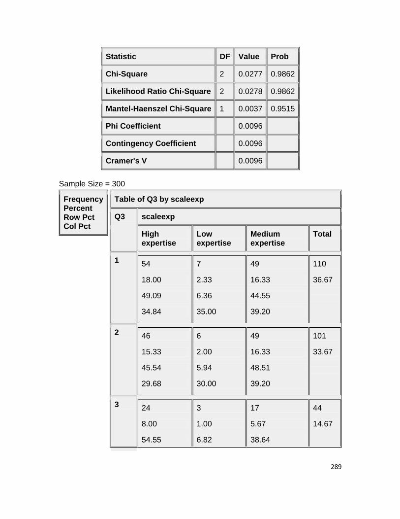
289

Statistic DF Value Prob

Chi-Square 2 0.0277 0.9862

Likelihood Ratio Chi-Square 2 0.0278 0.9862

Mantel-Haenszel Chi-Square 1 0.0037 0.9515

Phi Coefficient 0.0096

Contingency Coefficient 0.0096

Cramer's V 0.0096

Sample Size = 300

Frequency Percent Row Pct Col Pct

Table of Q3 by scaleexp

Q3 scaleexp

High expertise

Low expertise

Medium expertise

Total

1 54

18.00

49.09

34.84

7

2.33

6.36

35.00

49

16.33

44.55

39.20

110

36.67

2 46

15.33

45.54

29.68

6

2.00

5.94

30.00

49

16.33

48.51

39.20

101

33.67

3 24

8.00

54.55

3

1.00

6.82

17

5.67

38.64

44

14.67

290

15.48

15.00

13.60

4 31

10.33

68.89

20.00

4

1.33

8.89

20.00

10

3.33

22.22

8.00

45

15.00

Total 155

51.67

20

6.67

125

41.67

300

100.00

Statistics for Table of Q3 by scaleexp

Statistic DF Value Prob

Chi-Square 6 9.4936 0.1477

Likelihood Ratio Chi-Square 6 10.0343 0.1232

Mantel-Haenszel Chi-Square 1 5.6252 0.0177

Phi Coefficient 0.1779

Contingency Coefficient 0.1751

Cramer's V 0.1258

Sample Size = 300

Frequency Percent Row Pct Col Pct

Table of Q4 by scaleexp

Q4 scaleexp

High expertise

Low expertise

Medium expertise

Total

1 109

36.33

15

5.00

104

34.67

228

76.00

291

47.81

70.32

6.58

75.00

45.61

83.20

2 39

13.00

65.00

25.16

3

1.00

5.00

15.00

18

6.00

30.00

14.40

60

20.00

3 0

0.00

0.00

0.00

1

0.33

50.00

5.00

1

0.33

50.00

0.80

2

0.67

4 7

2.33

70.00

4.52

1

0.33

10.00

5.00

2

0.67

20.00

1.60

10

3.33

Total 155

51.67

20

6.67

125

41.67

300

100.00

Statistics for Table of Q4 by scaleexp

Statistic DF Value Prob

Chi-Square 6 14.4310 0.0252

Likelihood Ratio Chi-Square 6 12.3796 0.0540

Mantel-Haenszel Chi-Square 1 5.0816 0.0242

Phi Coefficient 0.2193

292

Statistic DF Value Prob

Contingency Coefficient 0.2142

Cramer's V 0.1551

WARNING: 50% of the cells have expected counts less than 5. Chi-Square may not be a valid test.

Sample Size = 300

Frequency Percent Row Pct Col Pct

Table of Q5 by scaleexp

Q5 scaleexp

High expertise

Low expertise

Medium expertise

Total

1 3

1.00

30.00

1.94

3

1.00

30.00

15.00

4

1.33

40.00

3.20

10

3.33

2 44

14.67

51.76

28.39

3

1.00

3.53

15.00

38

12.67

44.71

30.40

85

28.33

3 92

30.67

52.27

59.35

12

4.00

6.82

60.00

72

24.00

40.91

57.60

176

58.67

4 16 2 11 29

293

5.33

55.17

10.32

0.67

6.90

10.00

3.67

37.93

8.80

9.67

Total 155

51.67

20

6.67

125

41.67

300

100.00

Statistics for Table of Q5 by scaleexp

Statistic DF Value Prob

Chi-Square 6 10.7367 0.0969

Likelihood Ratio Chi-Square 6 7.3505 0.2896

Mantel-Haenszel Chi-Square 1 0.5925 0.4415

Phi Coefficient 0.1892

Contingency Coefficient 0.1859

Cramer's V 0.1338

WARNING: 25% of the cells have expected counts less than 5. Chi-Square may not be a valid test.

Sample Size = 300

Frequency Percent Row Pct Col Pct

Table of Q6 by scaleexp

Q6 scaleexp

High expertise

Low expertise

Medium expertise

Total

1 103

34.33

50.49

14

4.67

6.86

87

29.00

42.65

204

68.00

294

66.45

70.00

69.60

2 52

17.33

54.17

33.55

6

2.00

6.25

30.00

38

12.67

39.58

30.40

96

32.00

Total 155

51.67

20

6.67

125

41.67

300

100.00

Statistics for Table of Q6 by scaleexp

Statistic DF Value Prob

Chi-Square 2 0.3546 0.8375

Likelihood Ratio Chi-Square 2 0.3550 0.8374

Mantel-Haenszel Chi-Square 1 0.3201 0.5715

Phi Coefficient 0.0344

Contingency Coefficient 0.0344

Cramer's V 0.0344

Sample Size = 300

Frequency Percent Row Pct Col Pct

Table of Q1 by scaleW

Q1 scaleW

High trustworthiness

Low trustworthiness

Medium trustworthiness

Total

1 15

5.00

0

0.00

7

2.33

22

7.33

295

68.18

10.14

0.00

0.00

31.82

5.34

2 88

29.33

47.31

59.46

14

4.67

7.53

66.67

84

28.00

45.16

64.12

186

62.00

3 9

3.00

47.37

6.08

2

0.67

10.53

9.52

8

2.67

42.11

6.11

19

6.33

4 36

12.00

49.32

24.32

5

1.67

6.85

23.81

32

10.67

43.84

24.43

73

24.33

Total

148

49.33

21

7.00

131

43.67

300

100.00

Statistics for Table of Q1 by scaleW

Statistic DF Value Prob

Chi-Square 6 4.5204 0.6066

Likelihood Ratio Chi-Square 6 5.9185 0.4324

Mantel-Haenszel Chi-Square 1 0.2049 0.6508

296

Statistic DF Value Prob

Phi Coefficient 0.1228

Contingency Coefficient 0.1218

Cramer's V 0.0868

Sample Size = 300

Frequency Percent Row Pct Col Pct

Table of Q2 by scaleW

Q2 scaleW

High trustworthiness

Low trustworthiness

Medium trustworthiness

Total

1 93

31.00

53.14

62.84

9

3.00

5.14

42.86

73

24.33

41.71

55.73

175

58.33

2 55

18.33

44.00

37.16

12

4.00

9.60

57.14

58

19.33

46.40

44.27

125

41.67

Total

148

49.33

21

7.00

131

43.67

300

100.00

Statistics for Table of Q2 by scaleW

Statistic DF Value Prob

Chi-Square 2 3.6715 0.1595

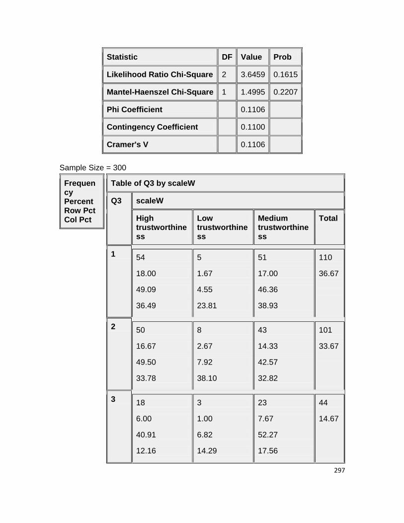
297

Statistic DF Value Prob

Likelihood Ratio Chi-Square 2 3.6459 0.1615

Mantel-Haenszel Chi-Square 1 1.4995 0.2207

Phi Coefficient 0.1106

Contingency Coefficient 0.1100

Cramer's V 0.1106

Sample Size = 300

Frequency Percent Row Pct Col Pct

Table of Q3 by scaleW

Q3 scaleW

High trustworthiness

Low trustworthiness

Medium trustworthiness

Total

1 54

18.00

49.09

36.49

5

1.67

4.55

23.81

51

17.00

46.36

38.93

110

36.67

2 50

16.67

49.50

33.78

8

2.67

7.92

38.10

43

14.33

42.57

32.82

101

33.67

3 18

6.00

40.91

12.16

3

1.00

6.82

14.29

23

7.67

52.27

17.56

44

14.67

298

4 26

8.67

57.78

17.57

5

1.67

11.11

23.81

14

4.67

31.11

10.69

45

15.00

Total

148

49.33

21

7.00

131

43.67

300

100.00

Statistics for Table of Q3 by scaleW

Statistic DF Value Prob

Chi-Square 6 6.0247 0.4204

Likelihood Ratio Chi-Square 6 6.1289 0.4089

Mantel-Haenszel Chi-Square 1 0.6941 0.4048

Phi Coefficient 0.1417

Contingency Coefficient 0.1403

Cramer's V 0.1002

Sample Size = 300

Frequency Percent Row Pct Col Pct

Table of Q4 by scaleW

Q4 scaleW

High trustworthiness

Low trustworthiness

Medium trustworthiness

Total

1 114

38.00

16

5.33

98

32.67

228

76.00

299

50.00

77.03

7.02

76.19

42.98

74.81

2 30

10.00

50.00

20.27

4

1.33

6.67

19.05

26

8.67

43.33

19.85

60

20.00

3 0

0.00

0.00

0.00

1

0.33

50.00

4.76

1

0.33

50.00

0.76

2

0.67

4 4

1.33

40.00

2.70

0

0.00

0.00

0.00

6

2.00

60.00

4.58

10

3.33

Total

148

49.33

21

7.00

131

43.67

300

100.00

Statistics for Table of Q4 by scaleW

Statistic DF Value Prob

Chi-Square 6 7.8370 0.2503

Likelihood Ratio Chi-Square 6 6.4002 0.3799

Mantel-Haenszel Chi-Square 1 0.7277 0.3936

300

Statistic DF Value Prob

Phi Coefficient 0.1616

Contingency Coefficient 0.1596

Cramer's V 0.1143

WARNING: 58% of the cells have expected counts less than 5. Chi-Square may not be a valid test.

Sample Size = 300

Frequency Percent Row Pct Col Pct

Table of Q5 by scaleW

Q5 scaleW

High trustworthiness

Low trustworthiness

Medium trustworthiness

Total

1 5

1.67

50.00

3.38

1

0.33

10.00

4.76

4

1.33

40.00

3.05

10

3.33

2 48

16.00

56.47

32.43

3

1.00

3.53

14.29

34

11.33

40.00

25.95

85

28.33

3 86

28.67

48.86

58.11

12

4.00

6.82

57.14

78

26.00

44.32

59.54

176

58.67

301

4 9

3.00

31.03

6.08

5

1.67

17.24

23.81

15

5.00

51.72

11.45

29

9.67

Total

148

49.33

21

7.00

131

43.67

300

100.00

Statistics for Table of Q5 by scaleW

Statistic DF Value Prob

Chi-Square 6 9.5404 0.1454

Likelihood Ratio Chi-Square 6 8.8293 0.1834

Mantel-Haenszel Chi-Square 1 2.4984 0.1140

Phi Coefficient 0.1783

Contingency Coefficient 0.1756

Cramer's V 0.1261

WARNING: 33% of the cells have expected counts less than 5. Chi-Square may not be a valid test.

Sample Size = 300

Frequency Percent Row Pct Col Pct

Table of Q6 by scaleW

Q6 scaleW

High trustworthiness

Low trustworthiness

Medium trustworthiness

Total

1 102 13 89 204

302

34.00

50.00

68.92

4.33

6.37

61.90

29.67

43.63

67.94

68.00

2 46

15.33

47.92

31.08

8

2.67

8.33

38.10

42

14.00

43.75

32.06

96

32.00

Total

148

49.33

21

7.00

131

43.67

300

100.00

Statistics for Table of Q6 by scaleW

Statistic DF Value Prob

Chi-Square 2 0.4162 0.8121

Likelihood Ratio Chi-Square 2 0.4059 0.8163

Mantel-Haenszel Chi-Square 1 0.0342 0.8534

Phi Coefficient 0.0372

Contingency Coefficient 0.0372

Cramer's V 0.0372

Sample Size = 300

303

Level of Trustworthiness by NGO

The FREQ Procedure

Frequen

cy

Percent

Row Pct

Col Pct

Table of NGO by scaleW

NGO scaleW

High

trustworthine

ss

Low

trustworthine

ss

Medium

trustworthine

ss

Total

Both 47

15.67

47.00

31.76

6

2.00

6.00

28.57

47

15.67

47.00

35.88

100

33.33

PAD

D

50

16.67

50.00

33.78

4

1.33

4.00

19.05

46

15.33

46.00

35.11

100

33.33

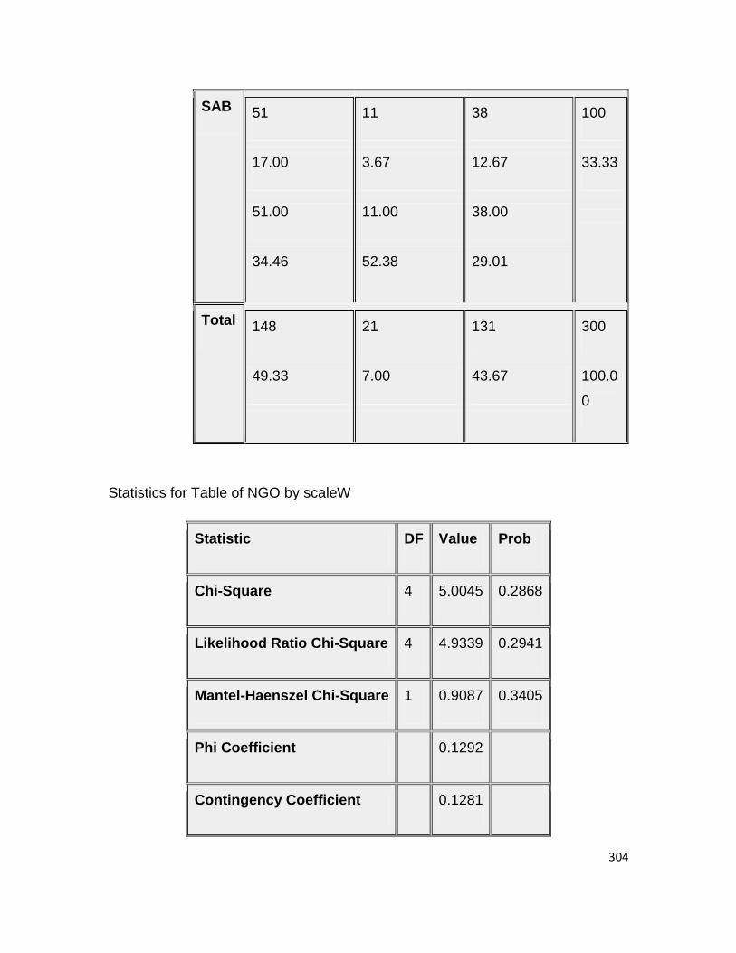
304

SAB 51

17.00

51.00

34.46

11

3.67

11.00

52.38

38

12.67

38.00

29.01

100

33.33

Total 148

49.33

21

7.00

131

43.67

300

100.0

0

Statistics for Table of NGO by scaleW

Statistic DF Value Prob

Chi-Square 4 5.0045 0.2868

Likelihood Ratio Chi-Square 4 4.9339 0.2941

Mantel-Haenszel Chi-Square 1 0.9087 0.3405

Phi Coefficient 0.1292

Contingency Coefficient 0.1281

305

Statistic DF Value Prob

Cramer's V 0.0913

Sample Size = 300

Level of Expertise by NGO

The FREQ Procedure

Frequency

Percent

Row Pct

Col Pct

Table of NGO by scaleexp

NGO scaleexp

High

expertise

Low

expertise

Medium

expertise

Total

Both 51

17.00

51.00

32.90

7

2.33

7.00

35.00

42

14.00

42.00

33.60

100

33.33

306

PADD 42

14.00

42.00

27.10

7

2.33

7.00

35.00

51

17.00

51.00

40.80

100

33.33

SAB 62

20.67

62.00

40.00

6

2.00

6.00

30.00

32

10.67

32.00

25.60

100

33.33

Total 155

51.67

20

6.67

125

41.67

300

100.00

Statistics for Table of NGO by scaleexp

Statistic DF Value Prob

Chi-Square 4 8.3199 0.0805

307

Statistic DF Value Prob

Likelihood Ratio Chi-Square 4 8.3771 0.0787

Mantel-Haenszel Chi-Square 1 2.3801 0.1229

Phi Coefficient 0.1665

Contingency Coefficient 0.1643

Cramer's V 0.1178

Sample Size = 300

308

Level of involvement and advertising effectiveness in NGO-corporate

partnerships

The FREQ Procedure

Frequency

Percent

Row Pct

Col Pct

Table of scale by SSec_D_1

scale SSec_D_1

1 2 Total

High involvement 50

16.67

48.54

42.74

53

17.67

51.46

28.96

103

34.33

Low involvement 8

2.67

30.77

6.84

18

6.00

69.23

9.84

26

8.67

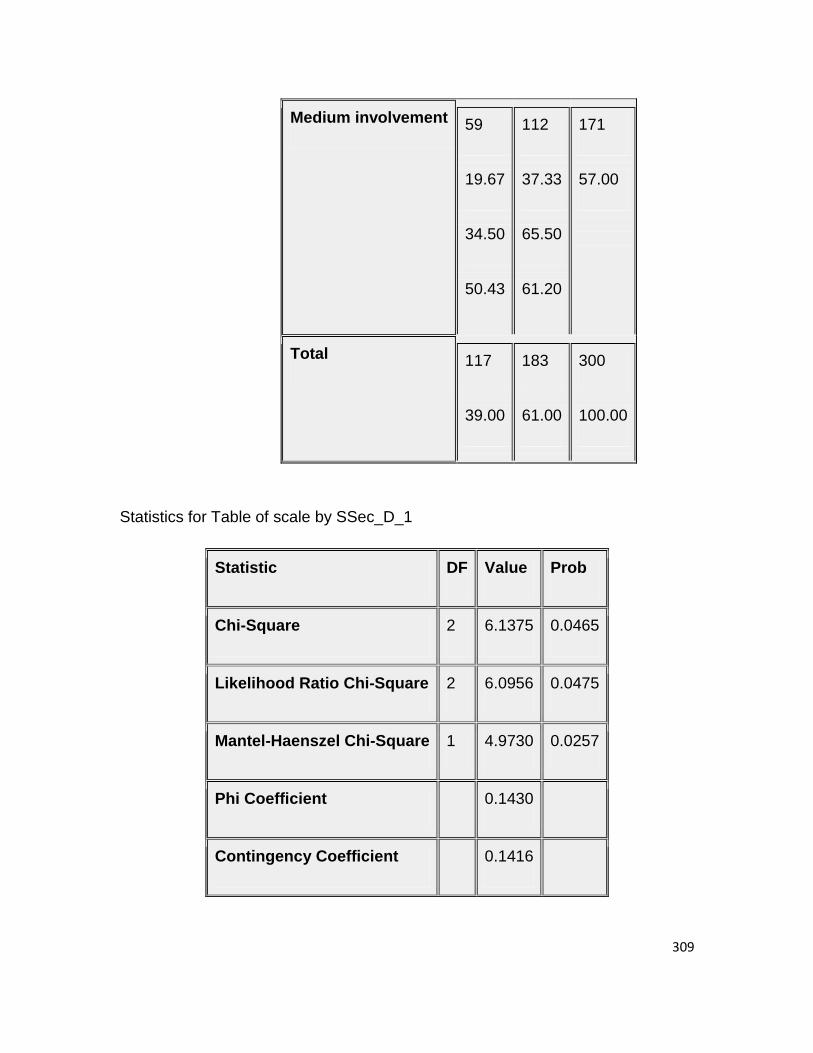
309

Medium involvement 59

19.67

34.50

50.43

112

37.33

65.50

61.20

171

57.00

Total 117

39.00

183

61.00

300

100.00

Statistics for Table of scale by SSec_D_1

Statistic DF Value Prob

Chi-Square 2 6.1375 0.0465

Likelihood Ratio Chi-Square 2 6.0956 0.0475

Mantel-Haenszel Chi-Square 1 4.9730 0.0257

Phi Coefficient 0.1430

Contingency Coefficient 0.1416

310

Statistic DF Value Prob

Cramer's V 0.1430

Sample Size = 300

Frequency

Percent

Row Pct

Col Pct

Table of scale by SSec_D_2

scale SSec_D_2

1 2 Total

High involvement 31

10.33

30.10

21.99

72

24.00

69.90

45.28

103

34.33

Low involvement 17

5.67

65.38

9

3.00

34.62

26

8.67

311

12.06

5.66

Medium involvement 93

31.00

54.39

65.96

78

26.00

45.61

49.06

171

57.00

Total 141

47.00

159

53.00

300

100.00

Statistics for Table of scale by SSec_D_2

Statistic DF Value Prob

Chi-Square 2 19.0864 <.0001

Likelihood Ratio Chi-Square 2 19.5200 <.0001

Mantel-Haenszel Chi-Square 1 13.9627 0.0002

Phi Coefficient 0.2522

312

Statistic DF Value Prob

Contingency Coefficient 0.2446

Cramer's V 0.2522

Sample Size = 300

Frequency

Percent

Row Pct

Col Pct

Table of scale by SSec_D_3

scale SSec_D_3

1 2 Total

High involvement 45

15.00

43.69

26.16

58

19.33

56.31

45.31

103

34.33

Low involvement 16

5.33

10

3.33

26

8.67

313

61.54

9.30

38.46

7.81

Medium involvement 111

37.00

64.91

64.53

60

20.00

35.09

46.88

171

57.00

Total 172

57.33

128

42.67

300

100.00

Statistics for Table of scale by SSec_D_3

Statistic DF Value Prob

Chi-Square 2 12.0416 0.0024

Likelihood Ratio Chi-Square 2 12.0101 0.0025

Mantel-Haenszel Chi-Square 1 11.4975 0.0007

314

Statistic DF Value Prob

Phi Coefficient 0.2003

Contingency Coefficient 0.1964

Cramer's V 0.2003

Sample Size = 300

Frequency

Percent

Row Pct

Col Pct

Table of scale by SSec_D_4

scale SSec_D_4

1 2 Total

High involvement 88

29.33

85.44

39.29

15

5.00

14.56

19.74

103

34.33

Low involvement 11 15 26

315

3.67

42.31

4.91

5.00

57.69

19.74

8.67

Medium involvement 125

41.67

73.10

55.80

46

15.33

26.90

60.53

171

57.00

Total 224

74.67

76

25.33

300

100.00

Statistics for Table of scale by SSec_D_4

Statistic DF Value Prob

Chi-Square 2 20.9312 <.0001

Likelihood Ratio Chi-Square 2 19.5179 <.0001

316

Statistic DF Value Prob

Mantel-Haenszel Chi-Square 1 3.8655 0.0493

Phi Coefficient 0.2641

Contingency Coefficient 0.2554

Cramer's V 0.2641

Sample Size = 300

Frequency

Percent

Row Pct

Col Pct

Table of scale by SSec_D_5

scale SSec_D_5

1 2 Total

High involvement 81

27.00

78.64

39.51

22

7.33

21.36

23.16

103

34.33

317

Low involvement 9

3.00

34.62

4.39

17

5.67

65.38

17.89

26

8.67

Medium involvement 115

38.33

67.25

56.10

56

18.67

32.75

58.95

171

57.00

Total 205

68.33

95

31.67

300

100.00

Statistics for Table of scale by SSec_D_5

Statistic DF Value Prob

Chi-Square 2 18.8099 <.0001

318

Statistic DF Value Prob

Likelihood Ratio Chi-Square 2 17.9344 0.0001

Mantel-Haenszel Chi-Square 1 2.7683 0.0961

Phi Coefficient 0.2504

Contingency Coefficient 0.2429

Cramer's V 0.2504

Sample Size = 300

Frequency

Percent

Row Pct

Col Pct

Table of scale by SSec_D_6

scale SSec_D_6

1 2 Total

High involvement 78

26.00

75.73

25

8.33

24.27

103

34.33

319

43.82

20.49

Low involvement 10

3.33

38.46

5.62

16

5.33

61.54

13.11

26

8.67

Medium involvement 90

30.00

52.63

50.56

81

27.00

47.37

66.39

171

57.00

Total 178

59.33

122

40.67

300

100.00

Statistics for Table of scale by SSec_D_6

Statistic DF Value Prob

320

Statistic DF Value Prob

Chi-Square 2 19.3511 <.0001

Likelihood Ratio Chi-Square 2 19.9807 <.0001

Mantel-Haenszel Chi-Square 1 12.8354 0.0003

Phi Coefficient 0.2540

Contingency Coefficient 0.2462

Cramer's V 0.2540

Sample Size = 300

Frequency

Percent

Row Pct

Col Pct

Table of scale by SSec_D_7

scale SSec_D_7

1 2 Total

High involvement 87

29.00

16

5.33

103

34.33

321

84.47

35.37

15.53

29.63

Low involvement 22

7.33

84.62

8.94

4

1.33

15.38

7.41

26

8.67

Medium involvement 137

45.67

80.12

55.69

34

11.33

19.88

62.96

171

57.00

Total 246

82.00

54

18.00

300

100.00

Statistics for Table of scale by SSec_D_7

322

Statistic DF Value Prob

Chi-Square 2 0.9557 0.6201

Likelihood Ratio Chi-Square 2 0.9663 0.6168

Mantel-Haenszel Chi-Square 1 0.8664 0.3520

Phi Coefficient 0.0564

Contingency Coefficient 0.0564

Cramer's V 0.0564

Sample Size = 300

Frequency

Percent

Row Pct

Col Pct

Table of scale by SSec_D_8

scale SSec_D_8

1 2 Total

High involvement 65

21.67

38

12.67

103

34.33

323

63.11

40.88

36.89

26.95

Low involvement 8

2.67

30.77

5.03

18

6.00

69.23

12.77

26

8.67

Medium involvement 86

28.67

50.29

54.09

85

28.33

49.71

60.28

171

57.00

Total 159

53.00

141

47.00

300

100.00

Statistics for Table of scale by SSec_D_8

324

Statistic DF Value Prob

Chi-Square 2 9.8853 0.0071

Likelihood Ratio Chi-Square 2 10.0333 0.0066

Mantel-Haenszel Chi-Square 1 3.5000 0.0614

Phi Coefficient 0.1815

Contingency Coefficient 0.1786

Cramer's V 0.1815

Sample Size = 300

Frequency

Percent

Row Pct

Col Pct

Table of scale by SSec_D_9

scale SSec_D_9

1 2 Total

High involvement 69

23.00

34

11.33

103

34.33

325

66.99

41.07

33.01

25.76

Low involvement 17

5.67

65.38

10.12

9

3.00

34.62

6.82

26

8.67

Medium involvement 82

27.33

47.95

48.81

89

29.67

52.05

67.42

171

57.00

Total 168

56.00

132

44.00

300

100.00

Statistics for Table of scale by SSec_D_9

326

Statistic DF Value Prob

Chi-Square 2 10.4721 0.0053

Likelihood Ratio Chi-Square 2 10.5915 0.0050

Mantel-Haenszel Chi-Square 1 9.8392 0.0017

Phi Coefficient 0.1868

Contingency Coefficient 0.1837

Cramer's V 0.1868

Sample Size = 300

Frequency

Percent

Row Pct

Col Pct

Table of scale by SSec_D_10

scale SSec_D_10

1 2 Total

High involvement 53

17.67

50

16.67

103

34.33

327

51.46

39.55

48.54

30.12

Low involvement 12

4.00

46.15

8.96

14

4.67

53.85

8.43

26

8.67

Medium involvement 69

23.00

40.35

51.49

102

34.00

59.65

61.45

171

57.00

Total 134

44.67

166

55.33

300

100.00

Statistics for Table of scale by SSec_D_10

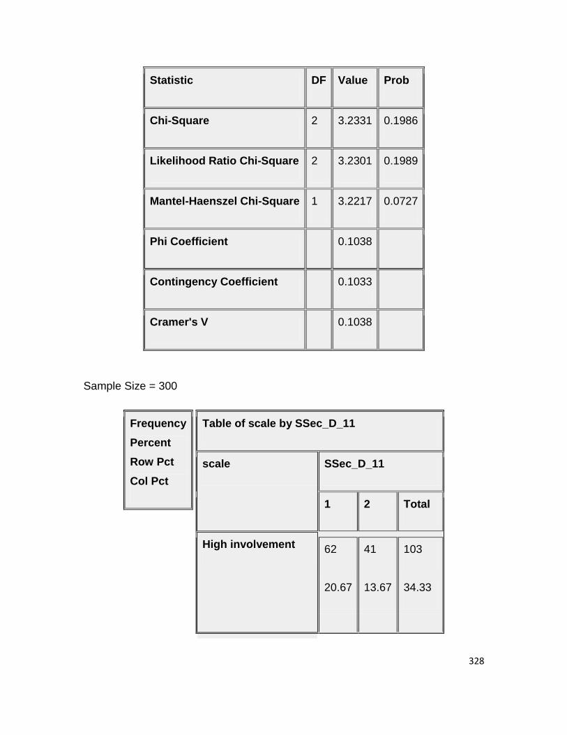
328

Statistic DF Value Prob

Chi-Square 2 3.2331 0.1986

Likelihood Ratio Chi-Square 2 3.2301 0.1989

Mantel-Haenszel Chi-Square 1 3.2217 0.0727

Phi Coefficient 0.1038

Contingency Coefficient 0.1033

Cramer's V 0.1038

Sample Size = 300

Frequency

Percent

Row Pct

Col Pct

Table of scale by SSec_D_11

scale SSec_D_11

1 2 Total

High involvement 62

20.67

41

13.67

103

34.33

329

60.19

41.06

39.81

27.52

Low involvement 7

2.33

26.92

4.64

19

6.33

73.08

12.75

26

8.67

Medium involvement 82

27.33

47.95

54.30

89

29.67

52.05

59.73

171

57.00

Total 151

50.33

149

49.67

300

100.00

Statistics for Table of scale by SSec_D_11

330

Statistic DF Value Prob

Chi-Square 2 10.0937 0.0064

Likelihood Ratio Chi-Square 2 10.3391 0.0057

Mantel-Haenszel Chi-Square 1 3.1205 0.0773

Phi Coefficient 0.1834

Contingency Coefficient 0.1804

Cramer's V 0.1834

Sample Size = 300

Frequency

Percent

Row Pct

Col Pct

Table of scale by SSec_D_12

scale SSec_D_12

1 2 Total

High involvement 73

24.33

30

10.00

103

34.33

331

70.87

39.46

29.13

26.09

Low involvement 9

3.00

34.62

4.86

17

5.67

65.38

14.78

26

8.67

Medium involvement 103

34.33

60.23

55.68

68

22.67

39.77

59.13

171

57.00

Total 185

61.67

115

38.33

300

100.00

Statistics for Table of scale by SSec_D_12

332

Statistic DF Value Prob

Chi-Square 2 11.8908 0.0026

Likelihood Ratio Chi-Square 2 11.7447 0.0028

Mantel-Haenszel Chi-Square 1 2.3219 0.1276

Phi Coefficient 0.1991

Contingency Coefficient 0.1953

Cramer's V 0.1991

Sample Size = 300

Frequency

Percent

Row Pct

Col Pct

Table of scale by SSec_D_13

scale SSec_D_13

1 2 Total

High involvement 84

28.00

19

6.33

103

34.33

333

81.55

41.38

18.45

19.59

Low involvement 10

3.33

38.46

4.93

16

5.33

61.54

16.49

26

8.67

Medium involvement 109

36.33

63.74

53.69

62

20.67

36.26

63.92

171

57.00

Total 203

67.67

97

32.33

300

100.00

Statistics for Table of scale by SSec_D_13

334

Statistic DF Value Prob

Chi-Square 2 20.4179 <.0001

Likelihood Ratio Chi-Square 2 20.5087 <.0001

Mantel-Haenszel Chi-Square 1 7.7787 0.0053

Phi Coefficient 0.2609

Contingency Coefficient 0.2524

Cramer's V 0.2609

Sample Size = 300