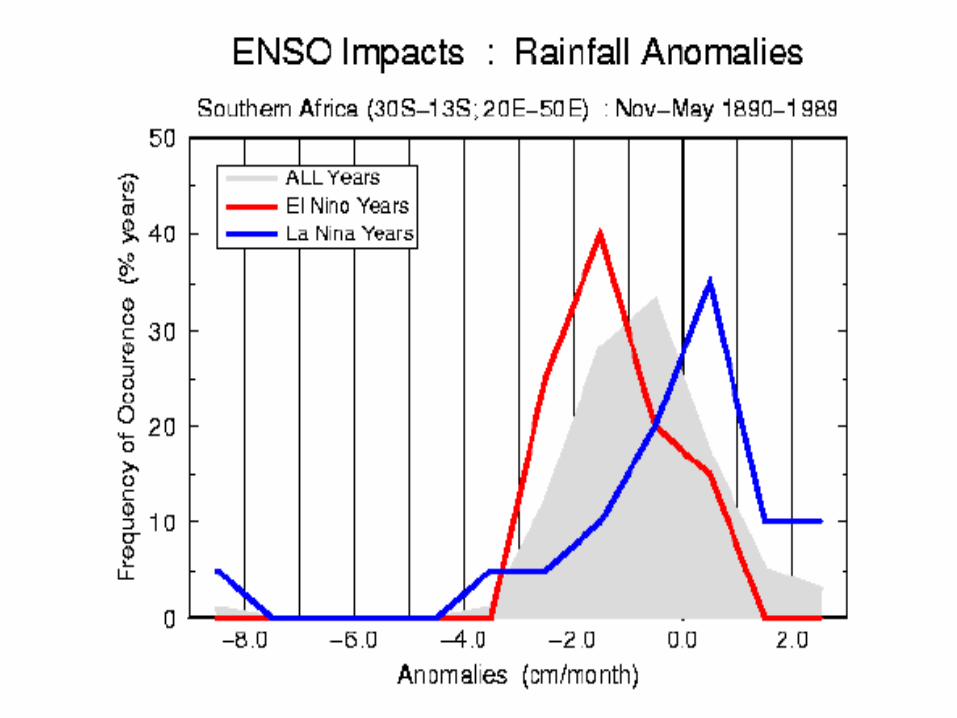
chaos: the enemy of seasonal forecasting! richard washington university of oxford...

Chaos:The enemy of seasonal

forecasting! Richard WashingtonUniversity of Oxford

[email protected]

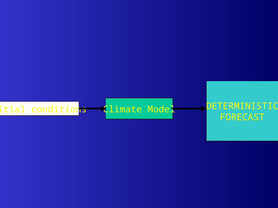
DETERMINISTICFORECAST

Climate ModelInitial conditions



E1

0

2

4

6

8

0 1 2 3 4 5 6 7 8 9

Tim e in Months



E1

0

2

4

6

8

0 1 2 3 4 5 6 7 8 9Tim e in Months

Realisation of weather will be different from observed After a few days…..



BEWARE THE BUTTERFLY!

Climate Model

Climate Model

Climate Model

Climate Model

Climate Model

Climate Model

Climate Model

Climate Model

Climate Model

Climate Model

Climate Model

Climate Model

Climate Model

Climate Model

Climate Model

Climate Model

Initial conditions

Initial conditions

Initial conditions

Initial conditions

Initial conditions

Initial conditions

Initial conditions

Initial conditions

ENSEMBLEFORECAST

Climate Model

Climate Model

Climate Model

Climate Model

Climate Model

Climate Model

Climate Model

Climate Model

Initial conditions

Initial conditions

Initial conditions

Initial conditions

Initial conditions

Initial conditions

Initial conditions

Initial conditions

0

1

2

3

4

5

6

7

8

9

0 1 2 3 4 5 6 7 8 9

Time in Months

E1

E2

E3

E4

0

1

2

3

4

5

6

7

8

0 1 2 3 4 5 6 7 8 9

Tim e in Months

E1

E2

E3

E4

Very LowSkill

Very HighSkill

Sensitivity to initial conditions…….

How can we better understand this?

The Game of Pinball

Is the trajectory of the ball predictable?

Is the system predictable?

How long will the ball stay on the board?

How many seconds does it take for the ball to vanish?

The system is fixed: nothing changes from the release of one ball to the next….

The gradient of the board is the same

The strength of the magnets is the same

The position of the magnets is the same

So, why is the system unpredictable?

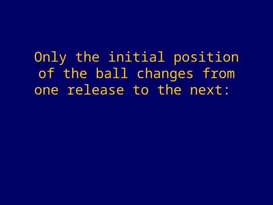
Only the initial position of the ball changes from one release to the next:

System is sensitive to initial conditions…….

The atmosphere in the mid latitudes never forgets the initial conditions

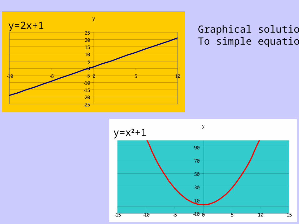
Understanding the problemgraphically……

y

-25

-20

-15

-10

-5

05

10

15

20

25

-10 -5 0 5 10

y=2x+1

y

-10

10

30

50

70

90

-15 -10 -5 0 5 10 15

y=x2+1

Graphical solutionsTo simple equations

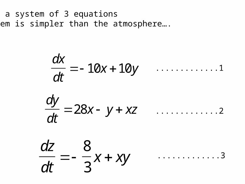
dx

dtx y 10 10

dy

dtx y xz 28

dz

dtx xy

8

3

.............1

.............2

.............3

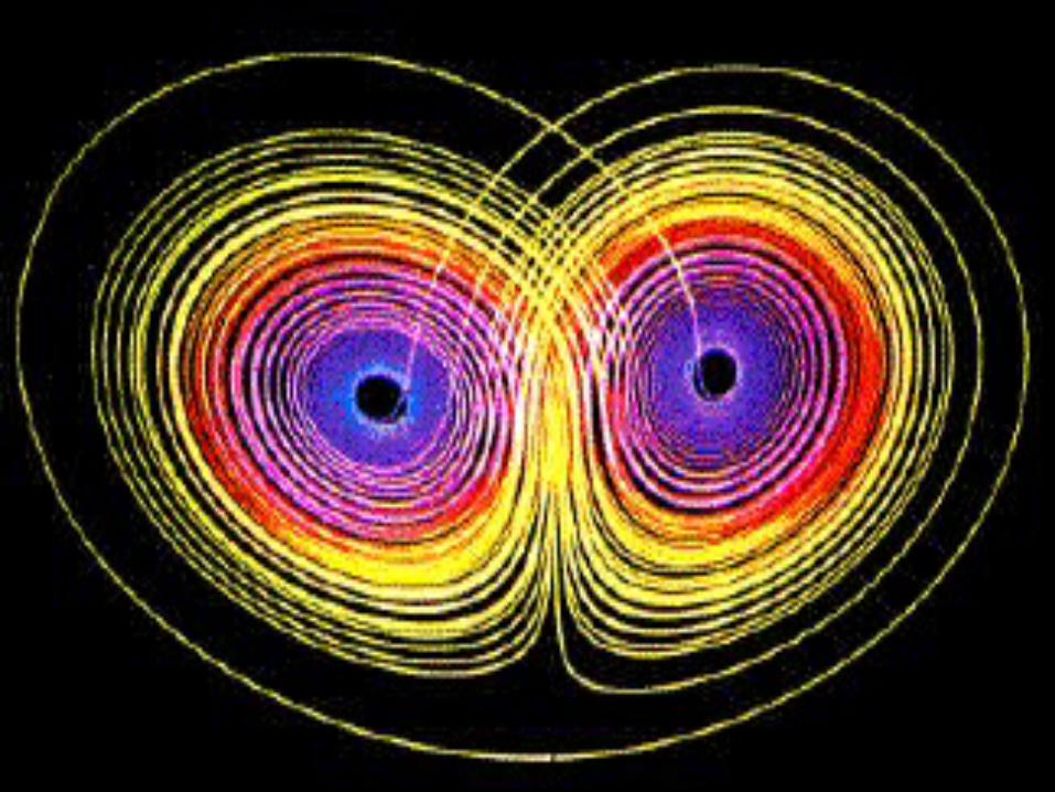
Take a system of 3 equationsSystem is simpler than the atmosphere….

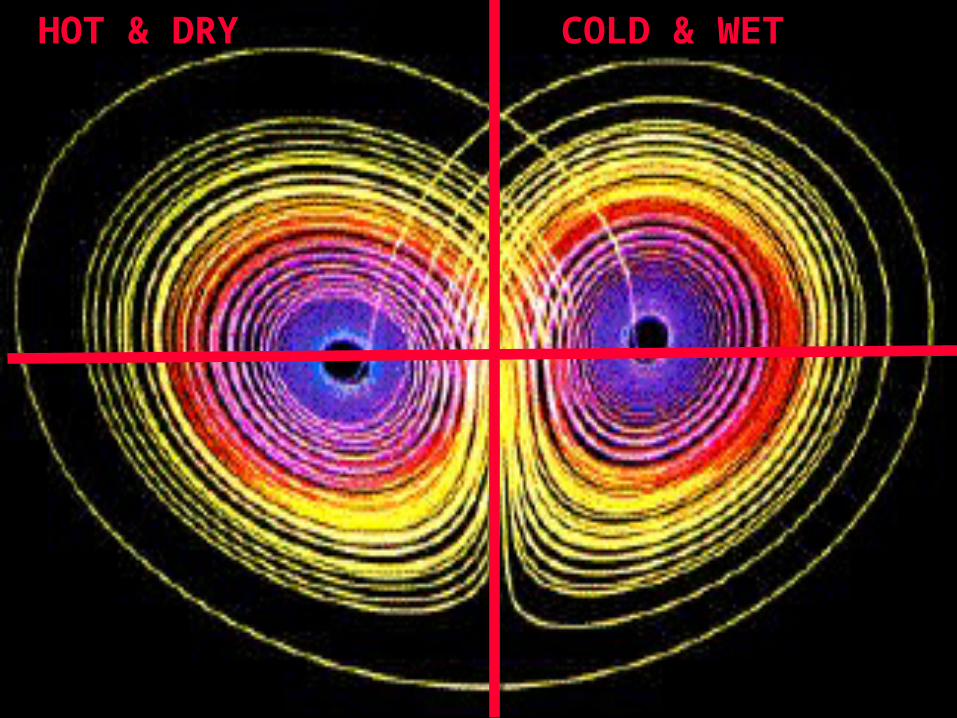
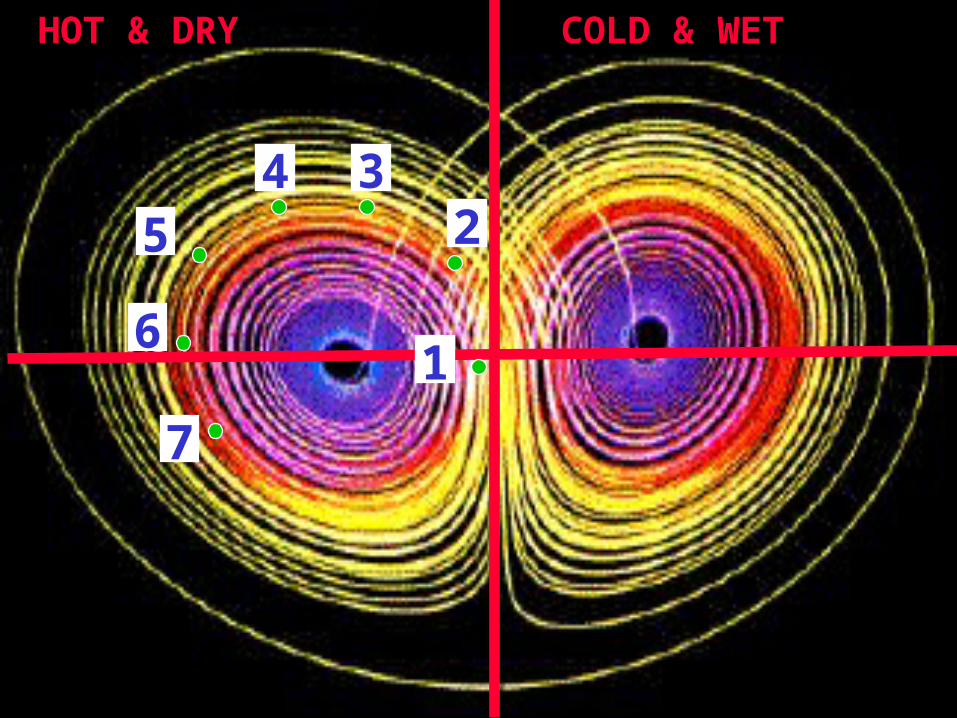
COLD & WETHOT & DRY

Evolution over 7 days……

COLD & WETHOT & DRY

1

2

3

4

5

67

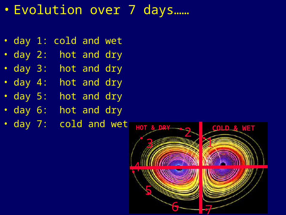
• Evolution over 7 days……

• day 1: cold and wet

• day 2: hot and dry





• day 7: cold and wet COLD & WETHOT & DRY

12

3

4

56 7

Evolution over 7 days……

Sensitivity to initial conditions

Experiment AEvolution over 7 days……

COLD & WETHOT & DRY

2

1

134

5

7

6


• day 1: hot and dry • day 2 hot and dry• day 3: hot and dry• day 4: hot and dry• day 5: hot and dry• day 6: hot and dry• day 7: hot and dry

Experiment BEvolution over 7 days……

COLD & WETHOT & DRY

2

1

3 45

6

7

Experiment A Experiment B















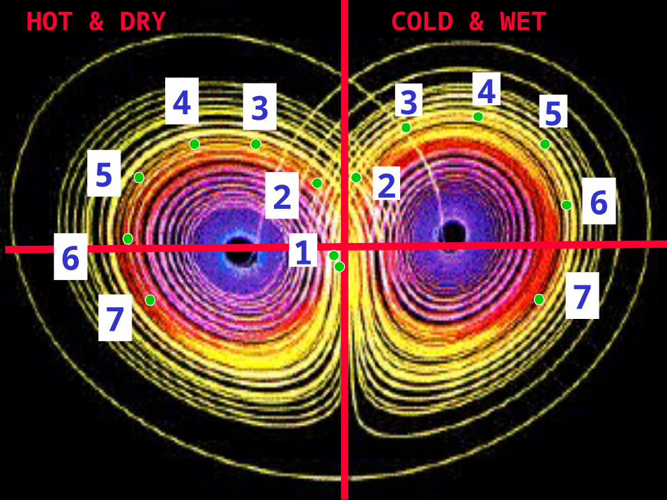
COLD & WETHOT & DRY

2

1

3 45

6

7

2

3

5

6

7

4

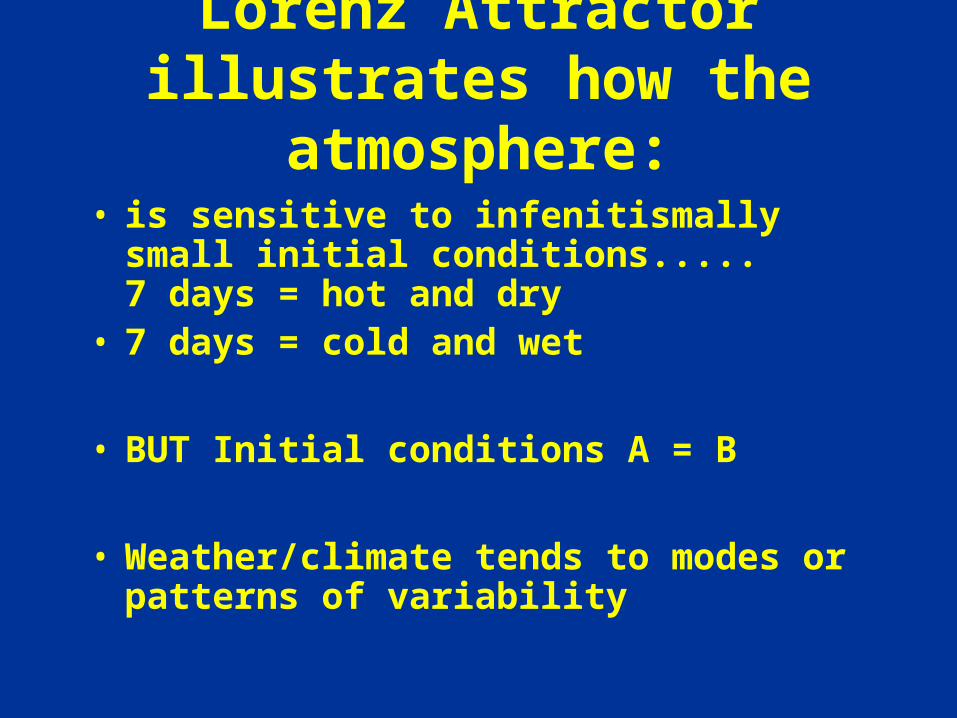
Lorenz Attractor illustrates how the atmosphere:

• is sensitive to infenitismally small initial conditions.....7 days = hot and dry

• 7 days = cold and wet

• BUT Initial conditions A = B

• Weather/climate tends to modes or patterns of variability

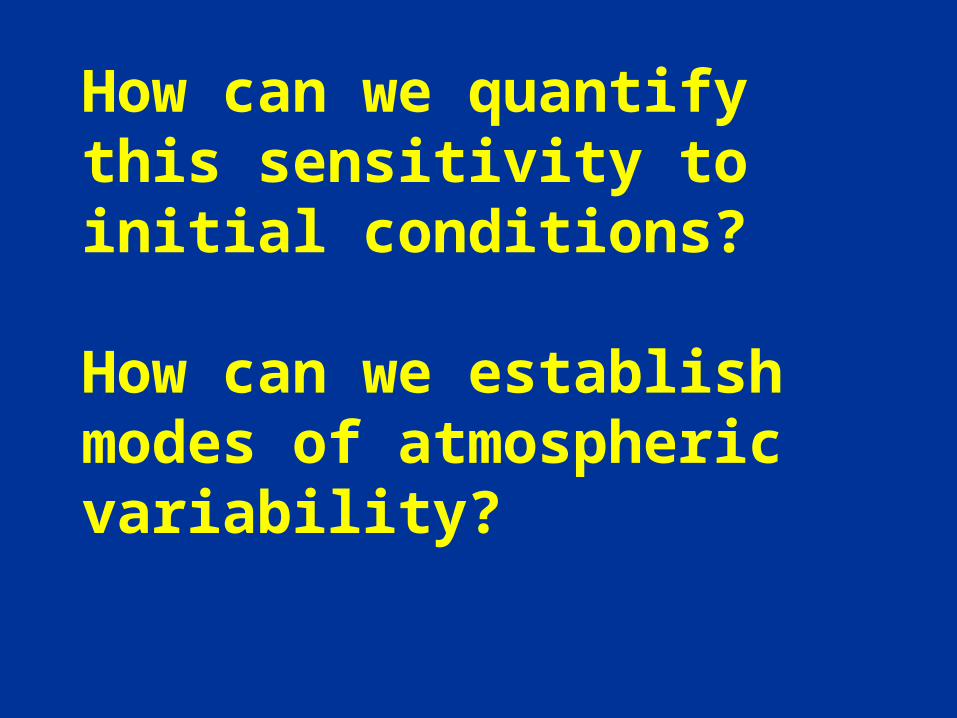
How can we quantify this sensitivity to initial conditions?

How can we establish modes of atmospheric variability?

How chaotic is the atmosphere?

Experimental Design- Pills and Patients

t1

t2

t3

t4

? ? ? ?

? ? ? ?

? ? ? ?

Experimental Design- Pills and Patients

t1

t2

t3

t4

RESULT????

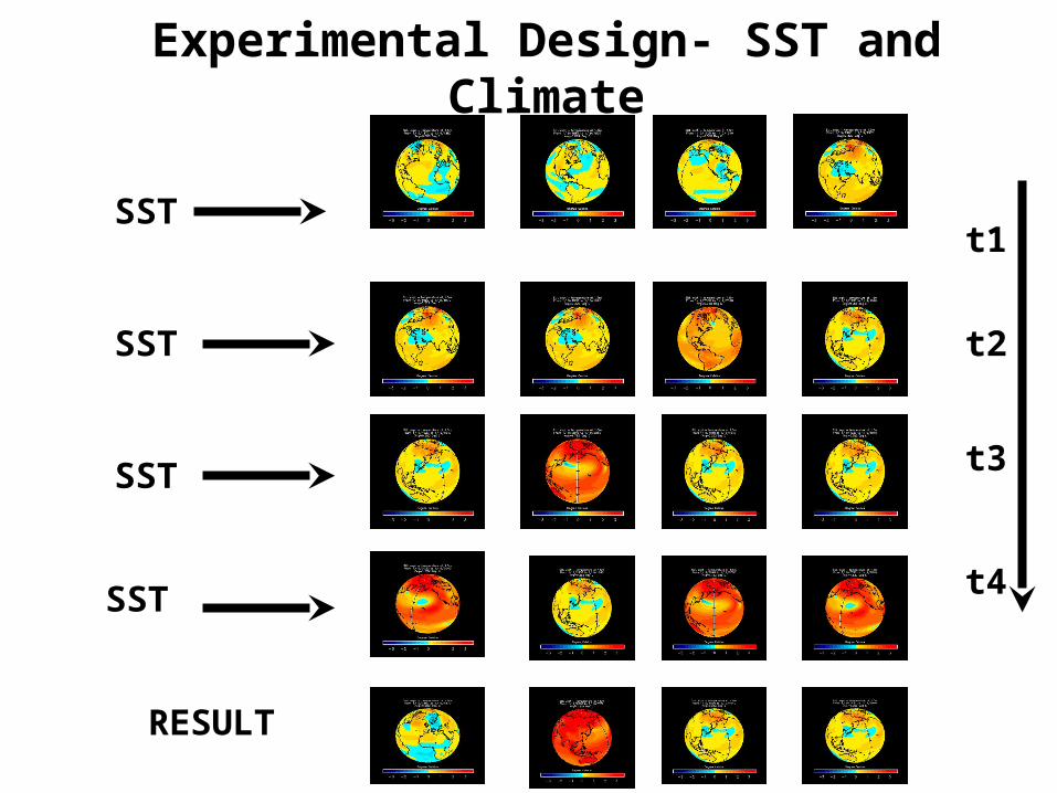
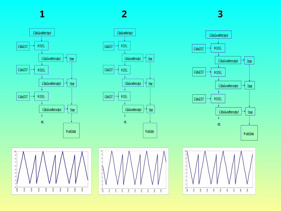
Experimental Design- SST and Climate

t1

t2

t3

t4

RESULT

SST

SST

SST

SST

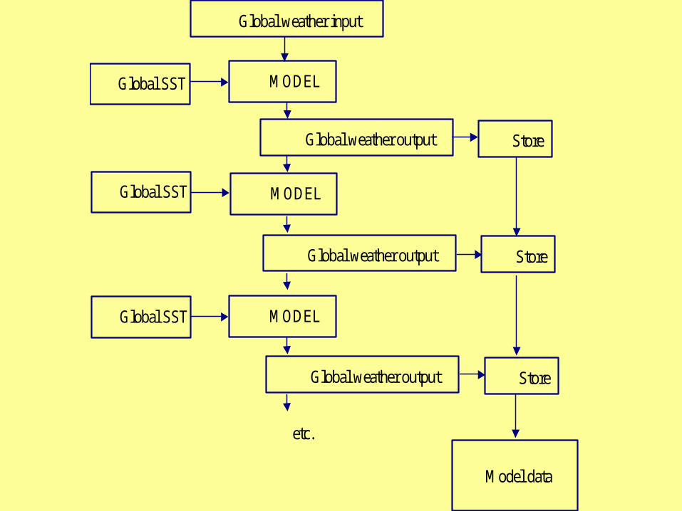
Global SST

Global SST

Global SST MODEL

MODEL

MODEL

Global weather output



Store

Store

Store

Model data

etc.

Global weather input

Global SST

Global SST

Global SST MODEL

MODEL

MODEL




Store

Store

Store

Model data

etc.


Global SST

Global SST

Global SST MODEL

MODEL

MODEL




Store

Store

Store

Model data

etc.


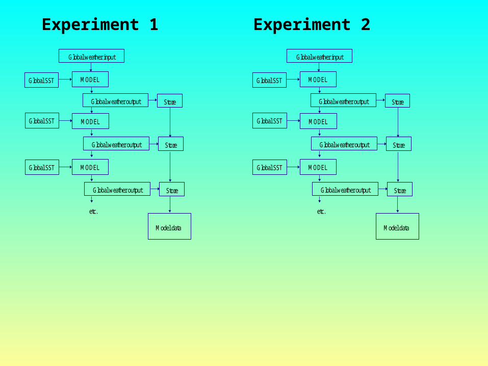
Experiment 1 Experiment 2

Global SST

Global SST

Global SST MODEL

MODEL

MODEL




Store

Store

Store

Model data

etc.


Global SST

Global SST

Global SST MODEL

MODEL

MODEL




Store

Store

Store

Model data

etc.


Global SST

Global SST

Global SST MODEL

MODEL

MODEL




Store

Store

Store

Model data

etc.


0

1

2

3

4

5

6

7

8

9

10

1900

1910

1920

1930

1940

1950

1960

1970

1980

1990

1 2 3

0

1

2

3

4

5

6

7

8

9

10

1900

1910

1920

1930

1940

1950

1960

1970

1980

1990

0

1

2

3

4

5

6

7

8

9

10

1900

1910

1920

1930

1940

1950

1960

1970

1980

1990

0

1

2

3

4

5

6

7

8

9

0 1 2 3 4 5 6 7 8 9

Time

E1

E2

E3

E4

0

1

2

3

4

5

6

7

8

0 1 2 3 4 5 6 7 8 9

Tim e

E1

E2

E3

E4

Very LowSkill

Very HighSkill

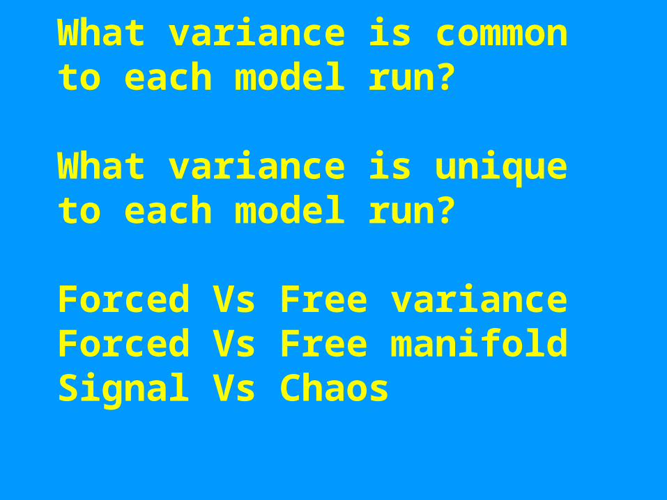
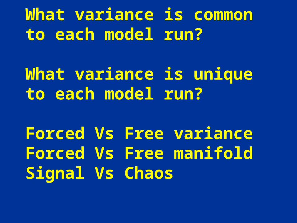
What variance is common to each model run?

What variance is unique to each model run?

Forced Vs Free varianceForced Vs Free manifoldSignal Vs Chaos

Simplest Case:Forced Vs Free Manifold

• single variable (rainfall)

• single model grid box

• Total Variance = forced variance + internal variability

Step 1: Estimate Internal Variability

computed as variance of each datum from its ensemble mean

N = number of years of forcing (92 years)n = number of experiments (6)

X = ensemble mean for ith year

2 2

11

1

1int

( )( )

N n

x xijj

n

i

N

Step 2: Estimate variance of ensemble means

computed as variance of the ensemble mean from the mean of all the data

2 2

1

1

1en

i

N

Nx x

( )

variance ensemble = variance due to forcing + 1/n variance due to internal variability

2 2 21en SST

n int

Step 3: Estimate variance due to Forcing by SST

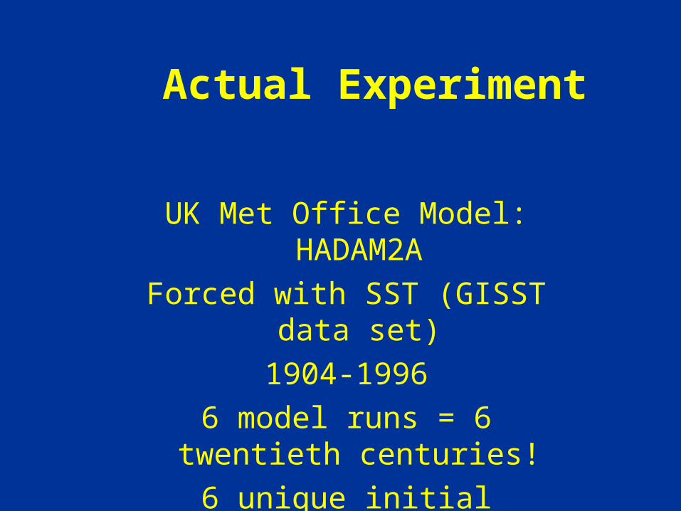
Actual Experiment

UK Met Office Model: HADAM2A

Forced with SST (GISST data set)

1904-1996

6 model runs = 6 twentieth centuries!

6 unique initial conditions

What variance is common to each model run?

What variance is unique to each model run?

Forced Vs Free varianceForced Vs Free manifoldSignal Vs Chaos

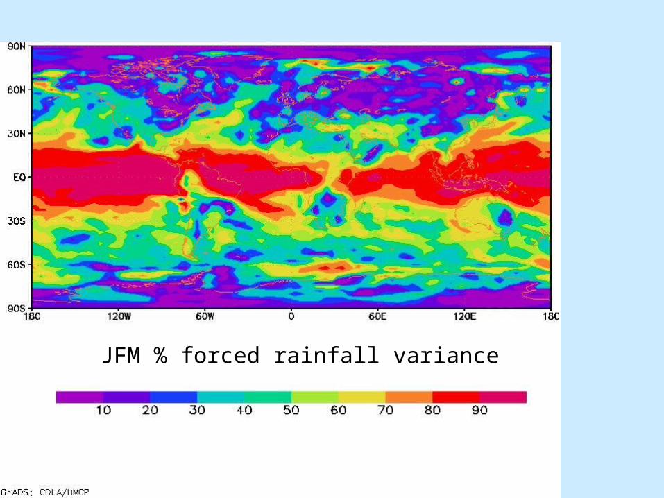
JFM % forced rainfall variance

JAS % forced rainfall variance

Chaos – the enemy of seasonal forecasting!

• Like many systems, the atmosphere is sensitive to initial conditions

• The same forcing due to SST can produce a different outcome if the starting conditions are different

• But the tropics is the least chaotic part of the atmosphere

• We can design methods to overcome the problem partially…e.g. ensemble forecasting

Readings

• Lorenz, E.N. 1995: The essence of chaos, UCL Press

• Rowell,-D.-P. et al 1995: Variability of summer rainfall over tropical north Africa (1906-92) : observations and modelling. Quarterly-Journal,-Royal-Meteorological-Society. 121(523), pp 669-704.

• Palmer T.N 1998: Nonlinear dynamics and climate change, Bulletin of the American Met Society, 79, 7, 1411-1423.

• Washington, R. 2000: Quantifying chaos in the atmosphere, Progress in Physical Geography.

chaos: the enemy of seasonal forecasting! richard washington university of oxford...

Documents

enemy of seasonal forecasting