changes in the profitability-growth relation and the ... · expenditures (barton and simko 2002,...
TRANSCRIPT
Changes in the Profitability-Growth Relation and the Implications for the Accrual
Anomaly
Meng Li
Submitted in partial fulfillment of the
requirements for the degree of
Doctor of Philosophy
under the Executive Committee
of the Graduate School of Arts and Sciences
COLUMBIA UNIVERSITY
2013

© 2013
Meng Li
All rights reserved
Abstract
Changes in the Profitability-Growth Relation and the Implications for the Accrual Anomaly
Meng Li
Valuation research establishes growth in net operating assets (∆NOA) as a primary
predictor of future profitability. The negative relation between ∆NOA and future profitability,
after controlling for current profitability, is researched extensively in the context of earnings
quality, capital investment, accounting conservatism, earnings management, and the accrual
anomaly. However, this study shows that while ∆NOA is negatively related to future profitability
from 1967 to 1995, it is positively related to future profitability from 1996 to 2010. The negative
effects of ∆NOA on future profitability (e.g., diminishing returns on investment, accruals
overstatement, and excess capitalization) continue to exist, although they are now dominated by
the positive implications of ∆NOA for future profitability. The positive relation between ∆NOA
and future profitability grows stronger over time for reasons including increasing intangible
intensity, increased volatility of economic activities, increased accounting conservatism,
accounting principles shifting toward a balance sheet/fair value approach, changing
characteristics of public firms, and the increasing importance of real options.
The change in the future profitability-∆NOA relation has important implications,
particularly for the accrual anomaly. The prevailing explanation for the anomaly is that an
increase (decrease) in NOA predicts a decrease (increase) in profitability and investors fail to
fully appreciate this negative relation. However, if this hypothesis is true, the anomaly should no
longer exist. I examine the anomaly over an extended time period, including more recent years,
and provide evidence that the anomaly is still present. To explain the persistence of the anomaly
over time, I conjecture and show that the market reaction to ∆NOA and the future profitability
implications of ∆NOA diverge throughout the sample period. Specifically, investors are always
over optimistic about the future profitability implications of the growth, i.e., in the first half of
the sample (1967-1988), investors do not fully react to the negative effects of growth on
profitability, and in the second half (1989-2010), they appear to over-emphasize the positive
implications of ∆NOA for future profitability. The anomaly weakens during periods when
investors’ reaction to ∆NOA aligns with the profitability implications of ∆NOA.

i
Table of Contents
ACKNOWLEDGEMENTS ......................................................................................................................................... III
DEDICATION ......................................................................................................................................................... IV
1. INTRODUCTION .................................................................................................................................................. 1
2. DATA DESCRIPTION ............................................................................................................................................ 6
3. THE RELATION BETWEEN GROWTH AND FUTURE PROFITABILITY ...................................................................... 8
3.1 A RE-EXAMINATION OF THE RELATION BETWEEN ∆NOA AND FUTURE PROFITABILITY ........................................................... 10
3.2 EXPLANATIONS FOR THE CHANGES IN THE RELATION BETWEEN ∆NOA AND FUTURE PROFITABILITY ......................................... 11
3.2.1 Factors driving the changes in βRNOA and β∆NOA ......................................................................................... 12 3.2.2 Empirical analysis of the factors driving the changes in βRNOA and β∆NOA .................................................. 22
3.3 ARE THE NEGATIVE EFFECTS OF ∆NOA STILL RELEVANT? ................................................................................................ 27
3.3.1 The negative relation between lagged ∆NOA and future profitability ...................................................... 28
3.3.2 The relation between components of ∆NOA and future profitability........................................................ 29
4. IMPLICATIONS FOR THE ACCRUAL ANOMALY .................................................................................................. 31
4.1 THE ACCRUAL ANOMALY OVER TIME ........................................................................................................................... 31
4.2 EXISTING EXPLANATIONS FOR THE ACCRUAL ANOMALY .................................................................................................. 34 4.3 HYPOTHESIZED EXPLANATION FOR THE ACCRUAL ANOMALY ............................................................................................ 35
4.3.1 Divergence between the market pricing and the profitability implications of ∆NOA ............................... 36
4.3.2 The possible role of lagged NOA in explaining the accrual anomaly ........................................................ 38
5. ROBUSTNESS TESTS.......................................................................................................................................... 40
6. CONCLUSION AND LIMITATIONS ...................................................................................................................... 42
REFERENCES ......................................................................................................................................................... 45
FIGURES ............................................................................................................................................................... 52
FIGURE 1: COEFFICIENTS FROM REGRESSING FUTURE PROFITABILITY ON GROWTH IN NET OPERATING ASSETS AND CURRENT
PROFITABILITY ............................................................................................................................................................. 52
FIGURE 2: THE PERSISTENCE OF RETURN ON NET OPERATING ASSETS .................................................................................... 55
FIGURE 3: COEFFICIENTS FROM THE FUTURE PROFITABILITY REGRESSION AND THE MEAN ANNUAL VOLATILITY ................................ 56 FIGURE 4: COEFFICIENT Β∆NOA OF THE HIGH VS. LOW GROUP OF FIRMS PARTITIONED BASED ON THE BOOK-TO-MARKET RATIO OF NET
OPERATING ASSETS EACH YEAR ........................................................................................................................................ 57
FIGURE 5: COEFFICIENT Β∆NOA OF THE HIGH VS. LOW GROUP OF FIRMS PARTITIONED BASED ON THE RATIO OF FIXED ASSETS TO AVERAGE
TOTAL ASSETS EACH YEAR ............................................................................................................................................... 58 FIGURE 6: COEFFICIENT (Β1) FROM REGRESSING FUTURE STOCK RETURN ON GROWTH IN NET OPERATING ASSETS AND CONTROL
VARIABLES .................................................................................................................................................................. 59
FIGURE 7: ANNUAL SIZE-ADJUSTED RETURN TO HEDGE PORTFOLIOS BASED ON THE GROWTH IN NET OPERATING ASSETS ................... 60 FIGURE 8: STANDARDIZED COEFFICIENTS FROM SEPARATE REGRESSIONS OF CONTEMPORANEOUS STOCK RETURN AND FUTURE
PROFITABILITY ON GROWTH IN NET OPERATING ASSETS AND CONTROL VARIABLES...................................................................... 61
TABLES ................................................................................................................................................................. 62
TABLE 1: DESCRIPTIVE STATISTICS ................................................................................................................................... 62 TABLE 2: REGRESSION OF FUTURE PROFITABILITY ON GROWTH IN NET OPERATING ASSETS AND CURRENT PROFITABILITY ................... 63
TABLE 3: FIRM CHARACTERISTICS OVER TIME ..................................................................................................................... 64
TABLE 4: TIME-SERIES CORRELATIONS (SPEARMAN ABOVE THE DIAGONAL, PEARSON BELOW) OF THE COEFFICIENTS FROM THE FUTURE
PROFITABILITY REGRESSION AND AVERAGE FIRM CHARACTERISTICS ......................................................................................... 66
ii
TABLE 5: TIME-SERIES REGRESSION OF THE COEFFICIENTS FROM THE FUTURE PROFITABILITY REGRESSION ON MEAN ANNUAL VOLATILITY
MEASURES .................................................................................................................................................................. 68 TABLE 6: REGRESSION OF FUTURE PROFITABILITY ON CURRENT AND LAGGED VALUES OF GROWTH IN NET OPERATING ASSETS,
CONTROLLING FOR CURRENT PROFITABILITY ....................................................................................................................... 70
TABLE 7: REGRESSION OF FUTURE PROFITABILITY ON COMPONENTS OF GROWTH IN NET OPERATING ASSETS, CONTROLLING FOR
CURRENT PROFITABILITY ................................................................................................................................................ 71 TABLE 8: REGRESSION OF FUTURE STOCK RETURN ON GROWTH IN NET OPERATING ASSETS AND CONTROL VARIABLES ....................... 72
TABLE 9: REGRESSION OF FUTURE STOCK RETURN ON COMPONENTS OF GROWTH IN NET OPERATING ASSETS AND CONTROL VARIABLES
................................................................................................................................................................................ 73
TABLE 10: TIME-SERIES REGRESSION OF MONTHLY RETURN ON A ZERO-INVESTMENT PORTFOLIO ON THE THREE FAMA AND FRENCH
(1993) FACTORS (MARKET RETURN, SIZE, AND B/M) AND MOMENTUM ................................................................................. 75
TABLE 11: REGRESSION OF CONTEMPORANEOUS STOCK RETURN ON GROWTH IN NET OPERATING ASSETS AND CONTROL VARIABLES ... 76
TABLE 12: REGRESSION OF CONTEMPORANEOUS STOCK RETURN ON COMPONENTS OF GROWTH IN NET OPERATING ASSETS AND
CONTROL VARIABLES ..................................................................................................................................................... 77
TABLE 13: REGRESSION OF FUTURE STOCK RETURN ON CURRENT AND LAGGED VALUES OF GROWTH IN NET OPERATING ASSETS AND
CONTROL VARIABLES ..................................................................................................................................................... 79
TABLE 14: REGRESSION OF FUTURE PROFITABILITY ON GROWTH IN NET OPERATING ASSETS AND CURRENT PROFITABILITY, USING
ALTERNATIVE MEASURES OF NET OPERATING ASSETS AND NET OPERATING PROFIT AFTER TAX ...................................................... 80
TABLE 15: REGRESSION OF FUTURE PROFITABILITY ON GROWTH IN NET OPERATING ASSETS AND CURRENT PROFITABILITY, EXCLUDING
BUSINESS COMBINATIONS .............................................................................................................................................. 81
TABLE 16: REGRESSION OF FUTURE PROFITABILITY ON GROWTH IN NET OPERATING ASSETS AND CURRENT PROFITABILITY, ALLOWING
DIFFERENT COEFFICIENTS FOR POSITIVE AND NEGATIVE GROWTH ........................................................................................... 82
APPENDIX ............................................................................................................................................................ 83
LITERATURE REVIEW ..................................................................................................................................................... 83

iii
Acknowledgements
I would like to thank my committee members Divya Anantharaman, Sharon Katz, Oded
Netzer, Doron Nissim (Sponsor), and Stephen Penman (Chair) for their guidance and support. I
also thank Colleen Honigsberg, Fabrizio Ferri, Dan Givoly, Trevor Harris, Alon Kalay, Urooj
Khan, Suresh Nallareddy, Jim Ohlson, Edward Riedl, Ayung Tseng, and workshop participants
at Boston University, Columbia University, George Mason University, and Penn State University
for their valuable comments and suggestions. All errors are mine.
I would like to express my sincere gratitude to Columbia Business School for the
wonderful opportunity, valuable support, and great experience that I gained during the years in
the doctoral program.

iv
Dedication
I dedicate this dissertation to my family for their love, support, and encouragement over
the many years, especially my late grandfather, my grandmother, my parents, and my uncle.
This thesis would not have been possible without the caring, patience, support, and
guidance of my advisor, Professor Nissim.
1
1. Introduction
The negative relation between growth in net operating assets (∆NOA) and future
profitability, after controlling for current profitability, is researched extensively in the context of
earnings quality, capital investment, accounting conservatism, earnings management, and the
accrual anomaly. However, ∆NOA also has positive implications for future profitability
attributable to the information of balance sheet about future performance and the increased
profitability generated by the growth. The positive relation is expected to grow stronger over
time given the accounting and economic changes in the last twenty years. As accounting
principles shift towards a balance sheet/fair value approach, the informativeness of book value
has increased over time. At the same time, the balance sheet accounts which capture the existing
resources that the firm may adopt for alternative uses provide more information about the firm’s
future performance when the business environment is more volatile and the overall profit level of
public firms is lower. As the economy shifts from being fixed assets oriented to being intangible
oriented, a given growth in net operating assets is associated with higher profitability than in the
past because of the profits contributed by the intangible investment.
I examine the relation between ∆NOA and future profitability, conditional on current
profitability, from 1967 to 2010. Consistent with prior literature, I find that the overall relation
between ∆NOA and future profitability is negative from 1967 to 1995. However, I show that
∆NOA positively predicts future profitability from 1996 onwards. The ability of current
profitability to predict future profitability declines monotonically during the 1980s and 1990s,
but it increases substantially during the 2000s.
The changes in the relation between ∆NOA and future profitability can be explained by
accounting changes, the increased volatility of economic activities, changes in the characteristics
2
of public firms, the increased importance of real option effects, and the increased intangible
intensity. Specifically, these factors result in a decrease in earnings persistence and an increase in
earnings volatility, stock return volatility, and the ability of book value to explain firm value.
Various measures of volatility—including stock return volatility, earnings volatility, and the
frequency of negative earnings, special items, and large special items (greater than 5% of
sales)—all increase substantially over time. I show that the ability of ∆NOA (current
profitability) to predict future profitability is positively (negatively) related to volatility levels.
Although the relation between ∆NOA and future profitability changes from negative to positive
for firms with all levels of intangible assets, the change is more pronounced for firms with higher
intangible intensity.
The changes in the overall relation between ∆NOA and future profitability do not
necessarily imply that the negative implications of growth for future profitability are no longer
relevant. The literature provides extensive evidence to explain the negative relation between
∆NOA and future profitability, conditional on current profitability.1 I show that the negative
effects of ∆NOA on future profitability continue to exist, although they are now dominated by
the positive implications resulting from the economic and accounting changes. The evidence
includes the following: (1) one- and two-year lagged ∆NOA are both negatively related to future
profitability in the second sub-period (1989-2010), even after controlling for current profitability
and current ∆NOA; and (2) decomposing ∆NOA, I find that the relation of working capital
accruals, depreciation, and the change in PP&E except depreciation to future profitability is
1 The explanations include earnings quality (Sloan 1996, Xie 2001, Richardson et al. 2005), the realization principle
and accounting conservatism (Givoly and Hayn 2000, Fairfield et al 2003, Penman and Zhang 2002), diminishing
returns on investment (Fairfield et al. 2003, Zhang 2007, Wu et al. 2010), and the excess capitalization of
expenditures (Barton and Simko 2002, Hirshleifer et al. 2004).
3
significantly negative for both sub-periods, while the relation of intangible growth and other
∆NOA to future profitability changes from negative to positive.
The changes in the relation between ∆NOA and future profitability have important
implications for the accrual anomaly. Sloan (1996) is the first to document the accrual anomaly.
He measures accruals as the change in non-cash working capital minus depreciation expense, and
he finds a negative relation between accruals and future stock returns. Fairfield et al. (2003)
extends Sloan (1996) by broadening the definition of accruals to include investments in long-
term net operating assets (long-term ∆NOA) and showing that both components of ∆NOA,
working capital accruals and long-term ∆NOA, are negatively related to future stock returns.
Following Fairfield et al. (2003), I refer to this broad measure of accruals in discussing the
accrual anomaly, i.e., the negative relation between ∆NOA and future stock returns.
The prevailing explanation for the accrual anomaly in the literature is that ∆NOA implies
a reduction in future profitability (e.g., Fairfield et al. 2003, Fama and French 2006), and
investors fail to fully appreciate this negative relation. The mispricing is corrected when future
earnings are announced. However, the finding of this study that the relation between ∆NOA and
future profitability is positive from 1996 onwards suggests that the anomaly should no longer
exist.
Indeed, a few recent studies (e.g., Richardson et al. 2010, Wu et al. 2010, Green et al.
2011) document that the accrual anomaly is insignificant during the mid 2000s. Given the
relatively short duration of their tested period, it is unclear whether the anomaly indeed
disappears.2 I examine the accrual anomaly from 1967 to 2010 (employing stock return data
through April 2012). The empirical evidence suggests that the anomaly is still present.
2 Studies show that other anomalies, such as the post earnings announcement drift, also do not perform well during
the mid 2000s (e.g., Richardson et al. 2010, Ayers et al. 2011).
4
Specifically, I find that (1) in the most recent several years, the anomaly resumes; (2) in the
1970s, there was a short period during which the accrual anomaly was insignificant and
exhibited a similar pattern to that found in the mid 2000s; (3) when the entire sample period is
divided into two equal length sub-periods, the change in the magnitude of the anomaly between
the two sub-periods is insignificant; and (4) all components of ∆NOA are significantly
negatively related to future stock returns and the strength of these relations does not change
during the sample period.
Considering that ∆NOA does not predict a reduction in future profitability in the second
sub-period, what could explain the persistence of the accrual anomaly throughout the sample
period? My empirical results suggest that risk contributes to the documented negative relation
between ∆NOA and future stock returns, but it is unlikely to fully explain it. I conjecture and
show that throughout the sample period the anomaly is related to the divergence between the
market reaction to ∆NOA and the future profitability implications of ∆NOA. Investors are
always over optimistic about the profitability implications of the growth. Specifically, in the first
half of the sample (1967-1988), investors do not fully react to the negative effects of growth on
profitability, and in the second half (1989-2010), they appear to over-extrapolate the positive
implications of ∆NOA for future profitability. Investors may over-emphasize the information
content of the book value of assets and liabilities. Consistent with this argument, Dichev et al.
(2012) reports that CFOs express concerns that “over-emphasis of the fair value approach is
misguided”.
The decline of the anomaly in the mid 2000s occurs during a period in which investors’
reaction to ∆NOA and the profitability implications of ∆NOA converge. The resumption of the
anomaly in the late 2000s can be explained by a divergence of market expectations and
5
profitability realizations, i.e., investors continue to react positively to ∆NOA while ∆NOA does
not positively predict future profitability. Considering that market pricing of ∆NOA has been
stable over the past twenty years, it is the profitability implications of ∆NOA that have been
shifting over time and cause the divergence. Future work exploring the accrual anomaly should
consider the movement of the profitability implications of ∆NOA.
By documenting changes in the relation between growth and future profitability and
linking them to economic and accounting factors, this study makes important contributions to
several strands of accounting and finance research. The profitability-growth relation has been
studied in the context of earnings quality, valuation, capital investment, accounting
conservatism, earnings management, and market efficiency. My findings suggest that growth
now provides different information regarding future profitability, and prior research inferences
that rely on the negative relation between growth and profitability should be reexamined. In the
context of the accrual anomaly, the prevailing explanation in the literature is that it reflects
investors’ failure to fully price the negative implications of growth for future profitability. I show
that while the anomaly is still related to the divergence between the market pricing of growth and
its profitability implications, in recent years it is driven by investors’ over-emphasis on the
positive implications of growth for future profitability.
The study continues as follows. Section 2 describes the sample data. Section 3
investigates the relation between ∆NOA and future profitability and explains the changes.
Section 4 examines the implications for the accrual anomaly. Section 5 conducts additional
analysis as robustness checks. Section 6 concludes.
6
2. Data Description
The sample used in this study consists of all firm-year observations that satisfy the
following criteria: (1) accounting data is available from COMPUSTAT, (2) the company fiscal
year end is in December, (3) total assets are at least 10 million USD in December 2011 prices,
(4) stock return data is available from the CRSP monthly return files, and (5) the firm is not a
financial institution or a utility company (GIC sector 40 or 55, respectively). I restrict the sample
to December fiscal year end firms to improve the comparability of the financial information in
the cross-section. Very small firms are excluded because their financial ratios often have
problematic distributions. Financial and utility firms are excluded from the sample because the
impact of regulation in both industries may constrain profitability, and the distinction between
operating and financing activities is not well-defined for financial firms. The sample spans 44
years, from 1967 to 2010, with stock return data employed through April 2012. The number of
annual observations ranges from 920 (for 1967) to 3,787 (for 1997). It increases monotonically
through 1997, and declines slightly afterwards. The total number of firm-year observations is
99,137.
The variables are measured as follows. Net operating assets are measured as total assets
minus operating liabilities.3 Operating liabilities are measured by subtracting debt in current
liabilities and long term debt from total liabilities. Growth in net operating assets (∆NOA) is
measured relative to average total assets, as in Fairfield et al. (2003). Working capital accruals
(∆WC) are estimated as the change in working capital minus depreciation, divided by average
3 An alternative approach is to exclude cash and marketable securities from total assets. I elected not to do so in the
primary analysis for several reasons: (a) at least a portion of the liquid funds is required for operations, and
estimating that portion is difficult; (b) risky operations require a greater “buffer” (e.g., to secure the availability of
cash to fund required investments in case financial markets dry up); (c) cash is often quite “sticky”, so the lost return
is recurring and should be accounted for; (d) related to the previous point, significant portions of the cash balances
of large corporations are held outside the U.S., and repatriating these funds would trigger significant tax payments.
In any case, as a robustness check, I verify that my results are not driven by this choice, as reported in Table 14.
7
total assets.4 Return on net operating assets (RNOA) is the ratio of net operating profit after tax
(NOPAT) to the net operating assets at the beginning of the period. NOPAT is calculated as net
income before extraordinary items and after minority interest, minus after-tax special items, plus
after-tax interest expense, plus minority interest in income. The tax adjustment is calculated by
multiplying pretax items by one minus the marginal tax rate. The marginal tax rate estimated is
as the top federal statutory tax rate in that year plus 2% (an estimate of the average incremental
effect of state taxes). Annual stock returns (RET) are measured from May through April of the
following year. Size-adjusted stock returns are calculated by deducting the average return of
firms in the same size-matched decile.
Beta is estimated using the 60 most recent monthly stock returns through April of the
following year (a minimum of 30 observations is required), and the total return on the S&P 500.
Idiosyncratic stock return volatility (Idio_Volat) is the residual volatility from the beta
regression. Size is measured as the log of the market value of equity on April 30 of the following
year. Book-to-market (BTM) is the ratio of book value of equity to the adjusted market value of
equity, calculated by multiplying the year end market value of equity by one plus the cumulative
stock return over the subsequent four months. The reason for this time adjustment is that year
end stock prices are not likely to fully reflect the value implications of the financial statement
information. Finally, to mitigate the impact of outliers, I trim each of the variables at the bottom
and top 1% of the empirical distribution each year. Table 1 presents summary statistics from the
pooled time-series cross-section distributions of the variables.
4 I use the balance sheet approach as in Sloan (1996) for measuring working capital accruals because cash flow
statement information is available only from 1988.
8
3. The relation between growth and future profitability
Financial statement analysis and valuation studies express future profitability and firm
value as a function of growth in net operating assets (∆NOA) and current profitability, with the
relative weights determined by the persistence of current earnings (Ou and Penman 1989,
Feltham and Ohlson 1995, Ohlson 1995, Fairfield et al. 2003). Many studies document a
conditional negative relation between ∆NOA (or components of ∆NOA) and future profitability.
In particular, Fairfield et al. (2003) shows that after controlling for current profitability, both
components of growth in net operating assets, working capital accruals and long-term ∆NOA,
have a negative association with one-year-ahead return on assets. Similarly, Fama and French
(2006) documents a negative relationship between working capital accruals and future
profitability and conclude that higher asset growth is associated with lower future profitability
after controlling for size, past profitability, and other fundamentals. Penman and Zhang (2006)
finds that the change in NOA is the primary variable for forecasting RNOA after including
current RNOA. The negative relation between ∆NOA and future profitability is explained from
different perspectives in accounting and finance research. Accounting and finance studies
attribute the negative relation between ∆NOA and future profitability to the following effects: (1)
working capital accruals imply low earnings quality (Sloan 1996, Xie 2001, Richardson et al.
2005); (2) ∆NOA reflects excess capitalization that leads to lower earnings and larger book
value, both of which imply a reduction in profitability (Barton and Simko 2002, Hirshleifer et al.
2004); (3) inter-temporal accounting biases depress earnings and accounting rates of return when
investment grows (Penman and Zhang 2002, Fairfield et al. 2003, Richardson et al. 2006); (4)
∆NOA reflects over-investment by some companies (Jensen 1986, Titman et al. 2004); and (5)
9
investment leads to a decline in average profitability due to diminishing returns on investment
(Fairfield et al. 2003p, Zhang 2007, Wu et al. 2010).
Despite extensive evidence and discussion about the negative relation between ∆NOA
and future profitability, ∆NOA has positive implications for future profitability because of the
information contained in balance sheet and the increased profitability associated with growth.
Over the last three decades, for both economic and accounting reasons, earnings volatility has
gradually increased and earnings persistence has declined (Givoly and Hayn 2000, Dichev and
Tang 2008), therefore book value provides more incremental information about firm value and
future performance. Relatedly, there has been a shift of value relevance from earnings to book
value (Collins et al. 1997, Francis and Schipper 1999), i.e., book value becomes more positively
related to price and value, while earnings’ relation with price and value becomes weaker. The
evidence suggests that the relation between ∆NOA which is a measure of the change in book
value and future profitability may become more positive over time. The profitability associated
with ∆NOA is higher than in the past because the profits are now contributed by both tangible
and intangible assets. Intangible assets become an increasingly important form of economic
resources in the recent decades. Motivated by the accounting and economic changes, this study
re-examines the ability of ∆NOA and current profitability to predict future profitability. I start by
re-examining the relation between ∆NOA and future profitability in Section 3.1. I describe and
perform empirical analysis on the factors that drive the temporal changes in the profitability-
growth relation in Section 3.2. I evaluate the continuing existence of negative effects of growth
on future profitability in Section 3.3.
10
3.1 A re-examination of the relation between ∆NOA and future profitability
Following Fairfield et al. (2003), I examine the conditional relation between ∆NOA and
future profitability using the following equation:
RNOAt+1 = β0 + β∆NOA ∆NOAt + βRNOA RNOAt + ε
In Table 2, I report summary statistics for the estimated coefficients from the cross-sectional
regression over the full sample period (1967-2010) as well as for two equal-length sub-periods
(1967-1988 and 1989-2010). β∆NOA is negative and significant for the full sample period, -0.0438
(t-stat=-4.0), which is consistent with the findings of existing literature. For the first sub-period,
1967-1988, which largely overlaps with the 1964-1993 sample period used in Fairfield et al.
(2003), the negative relation between ∆NOA and future profitability is particularly strong. β∆NOA
for this sub-period, -0.1040 (t-stat=-18.3), is more negative than the -0.05 average coefficient
reported in Fairfield et al. (2003), mainly because the sample used by Fairfield et al. (2003)
includes the years 1989-1993. However, for the second sub-period, 1989-2010, the relation is
insignificant: β∆NOA is 0.0164 (t-stat=1.5). The difference between β∆NOA in the two sub-periods
is highly significant, 0.1204 (t-stat=9.7). When the second sub-period is divided into two equal
length sub-periods, β∆NOA is -0.0149 (t-stat=-1.2) for the 1989-1999 period and 0.0425 (t-
stat=3.2) for the 2000-2010 period. The difference in β∆NOA for 1989-1999 and 2000-2010 is
highly significant (t-stat=3.1).
As expected, βRNOA is positive and highly significant in both sub-periods; however, it is
substantially smaller in the second sub-period. βRNOA declines from 0.7874 (t-stat=55.4) in the
first sub-period to 0.6166 (t-stat=18.2) in the second. This decline is statistically significant (t-
stat=-4.6). βRNOA for the first sub-period is comparable to the average coefficient of 0.78 in
Fairfield et al. (2003).
11
The time-series pattern of β∆NOA and βRNOA with a 95% confidence interval is plotted in
Figure 1. β∆NOA fluctuates around -0.1 during the years 1967-1985, increases to about -0.05
during the years 1986-1995, and is mostly positive after that. βRNOA is relatively stable around
0.8 during the years 1968-1983. It declines monotonically over the subsequent years, and it
reaches its minimum value of around 0.3 in 1999. After 2000, the coefficient rebounds to 0.7
where it is relatively stable for the remainder of the sample period.
3.2 Explanations for the changes in the relation between ∆NOA and future
profitability
What could explain the change in the sign of β∆NOA and the decline of βRNOA over time?
Because (1) stock prices reflect expected future profitability, (2) RNOA measures relative
earnings, and (3) ∆NOA is a change in book value, the decrease in βRNOA and the increase in
β∆NOA are consistent with the shift of value relevance from earnings to book value over time.5
Studies examining the value relevance of financial statement information (e.g., Collins et al.
1997, Francis and Schipper 1999, Givoly and Hayn 2000) document a substantial decline in the
incremental value relevance of earnings and a corresponding increase in the value relevance of
book value over time. The same forces that have caused the shift of value relevance from
earnings to book value likely explain the decrease in βRNOA and the increase in β∆NOA.
The reasons for the shift of value relevance from earnings to book value have been
discussed extensively in accounting research. The common drivers considered include the
volatility of economic activities, accounting changes, changing characteristics of public firms,
5 The change in the book value of net operating assets reflects operating accruals, other balance sheet accruals
related to non-operating events, and investments. Hribar and Collins (2002) makes the point that while balance sheet
accruals reflect earnings (e.g., an increase in accounts receivable from credit sales), they are also affected by non-
operating events such as mergers and acquisitions, divestitures, reclassifications, accounting changes and foreign
currency translations.
12
and real option effects. Economic and accounting changes have caused earnings to be more
volatile and less persistent. Public firms have become smaller, more volatile, less profitable, and
more growth oriented. The increase in earnings volatility and the decrease in earnings persistence
lead to the decline of βRNOA. The sign change of β∆NOA is attributable to the improved ability of
book value to predict profitability that results from accounting changes, economic changes
including increased economic volatility, changes in the characteristics of public firms, and
increased intangibles, and real options effects. The increasing emphasis on balance sheet/fair
value oriented accounting principles aligns book value to market value, thereby enhancing book
value’s ability to predict future profitability. From the perspective of real option valuation, the
value relevance of book value increases when profitability is low and volatile, because book
value measures the resources that can be liquidated or adapted for alternative uses. As business
operation shifts from being fixed assets oriented to intangible oriented, profits are generated by
both operating assets growth and intangibles. A unit of growth in net operating assets is now
associated with a higher level of profitability than in the past because of the profits contributed
by intangibles.
I discuss how these effects might affect βRNOA and β∆NOA in detail in Section 3.2.1. I
empirically relate βRNOA and β∆NOA to temporal changes in the firm characteristics, intangible
intensity, and accounting changes in Section 3.2.2.
3.2.1 Factors driving the changes in βRNOA and β∆NOA
In this section, I lay the groundwork for the empirical tests conducted in section 3.2.2. I
explain how economic changes, accounting changes, changing firm characteristics, and real
13
option effects may explain the temporal changes in β∆NOA and βRNOA, i.e., the change in the
relations of ∆NOA and RNOA with future profitability.
Economic changes
Economic volatility has increased substantially in recent decades, and caused earnings to
be more volatile and less persistent. βRNOA (the ability of current profitability to predict future
profitability) declines accordingly. The increase in economic volatility contributes to the rise of
β∆NOA because book value which captures the value of the firm’s resources is more informative
about future performance when business environment is more volatile. The intangible intensity
increases substantially over the past decades. The increased intangible intensity enhances the
positive relation between growth and future profitability by generating earnings that are more
volatile than that generated from traditional investment, and increasing the level of profitability
associated with unit growth. A given growth in net operating assets is now associated with
profits that are contributed by both tangible and intangible assets.
Technological innovations, changing economic conditions, and the growing demand for
global resources have caused significant changes in business operations. Using both financial
and real data, economic studies document that firm-level volatility has increased over the past
thirty years. For example, Campbell, Lettau, Malkiel, and Xu (2001) documents an increase in
the volatility of stock returns and real activities, and Comin and Mulani (2005, 2006) shows an
increase in the volatility of employment and sales growth. These changes in firm volatility are
associated with increased competition in product markets due to deregulation, technological
innovations, and easier access to capital markets (Chun et al. 2004, Comin and Mulani 2005,
Comin and Philippon 2005).
14
Lev and Zarowin (1999) provides empirical evidence that the business environment is
changing at an ever-increasing rate, and rapidly changing firms experience a larger increase in
R&D intensity than do stable firms. They attribute the documented decline in the
informativeness of earnings to the increasing pace of business change and the inadequacy of the
accounting system to reflect this change. Kothari et al. (2002) shows that earnings generated by
intangible assets are more volatile than that generated by traditional capital assets.
Consistent with the economic changes contributing to the increase in earnings volatility,
studies (Elliott and Shaw 1988, Francis et al. 1996) document an increase in the incidence and
magnitude of asset write-downs even prior to the adoption of the accounting standard mandating
the asset impairment test. Donelson et al. (2011) provides evidence on the role of economic
changes in explaining the observed increase in earnings volatility and the decline in earnings
persistence. They construct an index of economic activities that are frequently associated with
special items, and show that this index explains significant cross-sectional variation in the
incidence of special items.
Accounting changes
The rise of β∆NOA and the decline of βRNOA can also be related to increased accounting
conservatism and a shift of accounting principles towards the balance sheet approach. These
accounting changes have caused accounting earnings to be more volatile and less persistent, and
book value to be more relevant in explaining firm value. Givoly and Hayn (2000) provides
evidence of an increase in conservative financial reporting over time by documenting an increase
in earnings variability. Dichev and Tang (2008) documents a deterioration of matching over time
as a result of accounting and real economy evolution. They find a stark decline in earnings
persistence and a twofold increase in earnings volatility.
15
Since the mid 1980s, standard setters have increasingly adopted a balance sheet
perspective. Under the balance sheet approach, income reflects revisions in the value of assets
and liabilities rather than the difference between revenues and matched expenses. Nissim and
Penman (2008, page 13) points out that, under fair value accounting, “earnings are uninformative
about future earnings and about value; earnings are changes in value and as such do not predict
future value changes, nor do they inform about value (value ‘follows a random walk,’ as it is
said)”. The balance sheet approach, including fair value estimates, involves adjusting book value
to reflect future benefits that are expected to be realized. Book value produced under the balance
sheet approach is more closely aligned to market value and is a better indicator of future
profitability than that produced under the income statement approach.
Over the past decades, standard setters have gradually adopted the balance sheet
approach for many financial accounts, including impairment charges, goodwill and other
intangibles, most financial instruments, pension assets and liabilities, plan assets and obligations
under postretirement benefit programs, deferred taxes, asset retirement obligations, and other
items. Research findings generally suggest that the increasing adoption of the balance sheet
approach has improved the relevance of book value, increased earnings volatility, and reduced
earnings persistence (e.g., Barth 1994, Barth et al. 1995, 1996, 1998, Ayers 1998, Amir et al.
2001, 2010, Riedl 2004, Dechow and Ge 2006, Hann et al. 2007, Dichev and Tang 2008, Li et al.
2011). I next provide examples of the accounting changes and research findings regarding how
these accounting changes affect the ability of book value and current profitability to predict
future profitability. Five accounts are discussed: business combinations, postretirement benefits,
asset impairment, income taxes, and fair value accounting.
16
Business Combinations
Before 2001, two methods were used to account for business combinations: the purchase
method, and the pooling of interests method. Since 2001, firms are no longer allowed to use the
pooling method for new business combinations.6 In 2008, the FASB made significant changes in
the purchase method (referred to as the acquisition method under the new standard), which apply
for business combinations consummated after 2008.
Under all three methods—pooling, purchase and acquisition—the consolidation
procedure involves combining the accounts of the acquirer and the acquiree: revenues, expenses,
gains and losses in the income statement; cash flows in the cash flow statement; and assets and
liabilities on the balance sheet. The primary difference among the methods is in the measurement
basis.
Under the purchase method, the acquiree’s assets and liabilities are generally valued on
the consolidated balance sheet based on their estimated fair value at the business combination
date. If the amount that the acquirer paid for the acquiree’s common shares is more than the fair
value of the acquiree’s net identifiable assets (i.e., identifiable assets minus identifiable
liabilities), the excess is reported on the consolidated balance sheet as goodwill. In contrast,
under pooling the book values of the acquiree’s assets and liabilities are added to those of the
acquirer; there is no write-up of assets or recognition of goodwill. The presumption is that the
two firms have combined their operations but are otherwise operating as before, with the
stockholders of the two firms becoming stockholders in the combined entity. Thus, the purchase
method results in more informative measures of net operating assets.
6 The choice of combination method prior to 2001 was not discretionary. A number of specific conditions had to be
met for a transaction to be reported as pooling of interests. Two important requirements were: the acquirer must
issue voting common shares in exchange for at least 90% of the voting common stock of the acquiree, and the
acquisition must occur in a single transaction. Transactions that did not meet one or more of the criteria were
accounted for using the purchase method.
17
Starting in 2009, under the acquisition method, essentially all acquired assets and
liabilities, including goodwill, are fully marked-to-market. (Under the purchase method, some
asset and liabilities were reported at amounts different from fair value, and the fair value
adjustment was in proportion to parent’s ownership interest in subsidiary.)
Pension
SFAS 87 (1996) and SFAS 158 (2006) induce significantly more income volatility and
impair the value relevance of income, while the value relevance of book value is improved
(Hann et al. 2007). Hann et al. (2007) studies the value- and credit-relevance of financial
statements under fair-value versus smoothing models of pension accounting. They show that
fair-value pension accounting introduces considerable volatility in net income, reducing its
persistence and partially obscuring the underlying information in operating income. Fair-value
income is less value relevant than smoothing income because of its lower persistence, and the
fair value pension obligation on balance sheet is marginally more value relevant. Their evidence
suggests that the fair value pension accounting model impairs the value- and credit-relevance of
the combined financial statements unless transitory gains and losses are separated from more
persistent income components. They find that the fair-value model improves (impairs) the credit
relevance of balance sheet (income statement) numbers.
Asset impairment
SFAS No. 121, effective in 1996, was the first standard to explicitly address the
recognition and measurement of the impairment of long-lived assets, goodwill, and certain
18
identifiable intangibles.7 Prior to the issuance of SFAS No. 121, SFAS No. 5 Accounting for
Contingencies,8 had provided some general guidance in that it required firms to record losses
related to impaired assets, but the FASB Emerging Issues Task Force (EITF) noted that “there
were divergent measurement practices in accounting for impairment of assets.”. Riedl (2004)
shows that the incidence of write-downs increased significantly after the adoption of SFAS No.
121. SFAS No. 121 was superseded by SFAS No. 144 in 2002, but the general provisions were
retained. Asset write-downs reflect a change in the present value of the cash flows expected from
the asset, and should therefore serve to better align the book value to the market value. Indeed,
studies show that firms recording write-downs were performing poorly prior to the write-downs,
so by recording the write-downs managers were responding to economic changes (Elliott and
Shaw 1988, Francis et al. 1996, Rees et al. 1996).
While the increased recognition of write-downs may have improved the information
content of book value, it reduced earnings persistence. Riedl (2004) shows that “big bath”
reporting is more strongly associated with write-offs after SFAS No. 121. The significant
increase in earnings following a big bath (Haggard et al. 2011) reduces earnings persistence.
7 SFAS No. 121 “requires that long-lived assets and certain identifiable intangibles to be held and used by an entity
be reviewed for impairment whenever events or changes in circumstances indicate that the carrying amount of an
asset may not be recoverable. In performing the review for recoverability, the entity should estimate the future cash
flows expected to result from the use of the asset and its eventual disposition. If the sum of the expected future cash
flows (undiscounted and without interest charges) is less than the carrying amount of the asset, an impairment loss is
recognized. Otherwise, an impairment loss is not recognized. Measurement of an impairment loss for long-lived
assets and identifiable intangibles that an entity expects to hold and use should be based on the fair value of the
asset. … Examples of valuation techniques include the present value of estimated expected future cash flows using a
discount rate commensurate with the risks involved, option-pricing models, matrix pricing, option-adjusted spread
models, and fundamental analysis. … an impairment loss should be reported as a component of income from
continuing operations before income taxes…”
8 SFAS No. 5 “requires accrual by a charge to income (and disclosure) for an estimated loss from a loss contingency
if two conditions are met: (a) information available prior to issuance of the financial statements indicates that it is
probable that an asset had been impaired or a liability had been incurred at the date of the financial statements, and
(b) the amount of loss can be reasonably estimated. … In some cases, the carrying amount of an operating asset not
intended for disposal may exceed the amount expected to be recoverable through future use of that asset even
though there has been no physical loss or damage of the asset or threat of such loss or damage. … The question of
whether, in those cases, it is appropriate to write down the carrying amount of the asset to an amount expected to be
recoverable through future operations is not covered by this Statement.”
19
Information content of earnings is found to be impaired for firms reporting large negative special
items (Elliot and Hanna 1996).
SFAS No. 142 was issued in 2001 to supersede APB Opinion No. 17, Intangible Assets,
issued in 1970. SFAS No. 142 addresses financial accounting and reporting for acquired
goodwill and other intangible assets. Under SFAS No. 142, goodwill and intangible assets that
have indefinite useful lives are not amortized but instead are tested for impairment at least
annually. The FASB recognized that this standard may increase earnings volatility, but it argued
that the enhanced disclosures about goodwill and intangible assets will improve the financial
statement users’ ability to assess future profitability and cash flows. Goodwill impairment loss is
estimated from management’s projections of future cash flows of the business unit/asset-group,
and it is shown to be value relevant and a leading indicator of future profitability. Specifically, Li
et al. (2011) reports that investors and financial analysts revise downward their expectations of
value and earnings on the announcement of an impairment loss; goodwill impairment serves as a
leading indicator of a decline in future profitability. The results suggest that the recognition of
impairment charges improves the value relevance of book value.
Impairment of goodwill/unamortized intangibles, write-down/off of assets, and
restructuring charges are usually included in special items. The frequency and magnitude of
special items, especially negative special items, have increased dramatically over the past
decades (Elliot and Hanna 1996, Dechow and Ge 2006, Fairfield et al. 2009, Donelson et al.
2011, Johnson et al. 2011) due to both accounting and economic changes (Dichev and Tang
2008, Donelson et al. 2011). Large negative special items typically result from a balance sheet
perspective accounting that focuses on measuring assets and liabilities to reflect up-to-date
economic conditions. Earnings generated under balance sheet oriented accounting reflect the
20
change in the value of net assets during the period and are more volatile and less persistent.
Large negative special items are found to play an important role in explaining the low
persistence of earnings in low accrual firms (Dechow and Ge 2006).
Income taxes
Another example of the shift towards the balance sheet approach is the accounting for
income taxes. Effective for fiscal years beginning after December 15, 1992, SFAS No. 109
requires an “asset and liability” approach in accounting for income taxes. Deferred taxes are
considered assets and liabilities of the firm, and deferred tax expense is measured as the current
year change in net deferred tax liabilities, including adjustments to reflect changes in enacted tax
rates and in the expected realizability of deferred tax assets (using a valuation allowance).
Studies have shown that SFAS No. 109 increased the value relevance of deferred tax accounts.
Deferred tax components—deferred tax assets, valuation allowance, the adjustment of deferred
tax accounts for enacted tax rate changes, and the net realizable value of deferred taxes from
losses and credits carried forward—all provide value relevant information (Ayers 1998, Amir et
al. 2001, Amir et al. 2010). Valuation allowances are also informative about the realization of
deferred tax assets in the future and future taxable income (Kumar and Visvanathan 2003).
Fair value accounting
Fair value accounting9 is currently applied to all derivatives, most investments in fixed
income securities, and some investments in equity securities. The reported amounts of other
9 SFAS 115, effective for fiscal years beginning after December 15, 1993, addresses the accounting and reporting
for investments in equity securities that have readily determinable fair values and for all investments in debt
securities. Under this standard, investments are classified in three categories and accounted for as follows. Debt
securities that the enterprise has the positive intent and ability to hold to maturity are classified as held-to-maturity
21
financial instruments increasingly involve fair value considerations. Examples include options
and restricted stock, retained components from transferred financial assets and extinguished
liabilities, and financial instruments with characteristics of both liabilities and equity. Research
has generally shown that fair value estimates of investment securities provide significant
explanatory power beyond that provided by historical costs (Barth 1994, Barth et al. 1996,
Nelson 1996, etc.), and that fair value based earnings are more volatile than historical cost
earnings for economic reasons (Barth et al. 1995, Hodder et al. 2006).
Changing firm characteristics and real options
In conjunction with the economic and accounting changes, public firms have become
smaller, less profitable, and more growth oriented (Fama and French 2001). The value relevance
literature generally focuses on the changing characteristics of public firms as the primary
explanation for the shift of value relevance from earnings to book value. Collins et al. (1997)
attributes the shift of value relevance to the increasing frequency and magnitude of special items
and negative earnings, changes in average firm size, and the increase in intangible intensity.
These changes reduce earnings persistence and increase earnings volatility, i.e., special items
(Dechow and Ge 2006) and negative earnings (Hayn 1995) are relatively transitory, and
intangible-driven earnings are more volatile than earnings generated by other investments
(Kothari et al. 2002). Therefore, the ability of current profitability to predict future profitability
declines.
securities and reported at amortized cost. Debt and equity securities that are bought and held principally for the
purpose of selling them in the near term are classified as trading securities and reported at fair value, with unrealized
gains and losses included in earnings. Debt and equity securities not classified as either held-to-maturity or trading
are classified as available-for-sale and reported at fair value, with unrealized gains and losses excluded from
earnings and reported in a separate component of shareholders’ equity.”
22
These changes in firm characteristics also imply an increase in the value relevance of
book value through the real option effects. Burgstahler and Dichev (1997) demonstrates that the
relevance of book value increases when profitability is low. This is because book value captures
the value of existing resources, and the option to adopt existing resources for alternative use is
particularly valuable when profitability is low. In related work, Barth et al. (1998) shows that the
incremental explanatory power of equity book value (net income) increases (decreases) as
financial health decreases. The decline of average profitability (Fama and French 2001) therefore
implies an increase in the value relevance of book value. The value of real options also become
increasingly important because volatility has increased significantly over the past thirty years,
and volatility is the primary determinant of the value of real options (Grullon et al. 2011).
3.2.2 Empirical analysis of the factors driving the changes in βRNOA and β∆NOA
In this section, I empirically relate βRNOA and β∆NOA to temporal changes in firm
characteristics, intangible intensity, and accounting changes. I first show that relevant firm
characteristics, including stock return volatility, earnings volatility, sales growth volatility, the
frequency of negative earnings, the frequency of special items, and R&D intensity all have
changed systematically over the sample period. Both βRNOA and β∆NOA are highly correlated with
cross-sectional average values of these firm characteristics. In particular, βRNOA (β∆NOA) is
significantly positively (negatively) related to both stock return volatility, earnings volatility, and
sales growth volatility. The change of β∆NOA is more pronounced for intangible intensive firms.
Lastly, as an attempt to relate β∆NOA to specific accounting changes, I compare β∆NOA between
groups of firms that are expected to have different sensitivity to the accounting changes about
23
asset impairment and deferred taxes. However, the empirical evidence does not validate the
effects of accounting changes.
Temporal changes in firm characteristics
Table 3 presents the average values of select firm characteristics for both sub-periods, as
well as the change (with the related t-statistics) in the average values between the two sub-
periods. The average values of the characteristics are calculated for each sub-period as the time-
series means of the cross-sectional means (first panel of Table 3) or the cross-sectional medians
(second panel). The characteristics include stock return volatility, RNOA volatility, sales growth
volatility, an indicator variable for negative earnings, an indicator variable for special items, an
indicator variable for large special items (larger than 5% of sales), ∆NOA, RNOA, book-to-
market value of NOA, and R&D intensity.
As expected, the variables exhibit significant differences between the two sub-periods.
Stock return volatility, RNOA volatility, and sales growth volatility all increase significantly.
Stock return volatility increases from 0.1236 to 0.1584 (t-stat=5.7 for the difference), RNOA
volatility from 0.0418 to 0.1217 (t-stat=6.8 for the difference), and sales growth volatility from
0.1906 to 0.3402 (t-stat=7.0 for the difference). The proportion of negative earnings increases
from 0.1466 to 0.3641 (t-stat=9.6 for the difference). The proportion of non-zero (large) special
items increases from 0.1765 (0.0384) to 0.5309 (0.1624), and both changes are highly
significant. Average RNOA drops from 0.0949 in the first sub-period to 0.0008 in the second,
and the difference is highly significant (t-stat=-6.0). The change in the median value of RNOA is
smaller but still highly significant, from 0.0948 in the first period to 0.0698 in the second (t-
stat=-5.0 for the difference). Apparently, profitability has become strongly negatively skewed,
and so the importance of the adaptation and other downside-protection real options has
24
increased. The value of real options also proliferates because of the increase in intangible
intensity. The median R&D intensity increases from 0.0176 to 0.0474, and the difference is
significant (t-stat=8.0). The increase in mean R&D intensity is even larger, which is driven by
the R&D activities of start-up firms. The average book-to-market ratio of NOA declines
significantly, from 0.8418 to 0.6396, reflecting the increase in unrecognized intangibles.10
As discussed in the previous section, the rise of β∆NOA and the decline of βRNOA are
related to the lower persistence and higher volatility of profitability caused by economic and
accounting changes. The following analysis of the mean reverting pattern of profitability
demonstrates the decline in RNOA persistence and the increase in RNOA volatility. For each
sub-sample (1967-1988 and 1989-2010), ten equally-sized portfolios based on RNOA are formed
in each year (i.e., base year 0), and the median value of RNOA for each portfolio is calculated
for each of the years 0 through 10. Figure 2 plots the time-series medians (over all the base
years) of the portfolio median RNOA. As expected, the cross-sectional variation in RNOA is
substantially larger in the second sub-period, and the persistence of RNOA is substantially
smaller. The magnitude of RNOA reversion is much larger in the second period than the first
period for most of the portfolios.
Relating βRNOA and β∆NOA to the changes in firm characteristics
To determine whether the observed trends of β∆NOA and βRNOA can be explained by the
changes in firm characteristics, I perform correlation and regression analyses. Table 4 presents
the pair time-series correlation coefficients (Spearman above the diagonal, and Pearson below)
among β∆NOA, βRNOA, average values of the firm characteristics, and a time trend (year). The
10
Alternative explanations for the decline in the book-to-market ratio are increases in either current profitability or
current growth. However, average RNOA declines and average ∆NOA does not increase.
25
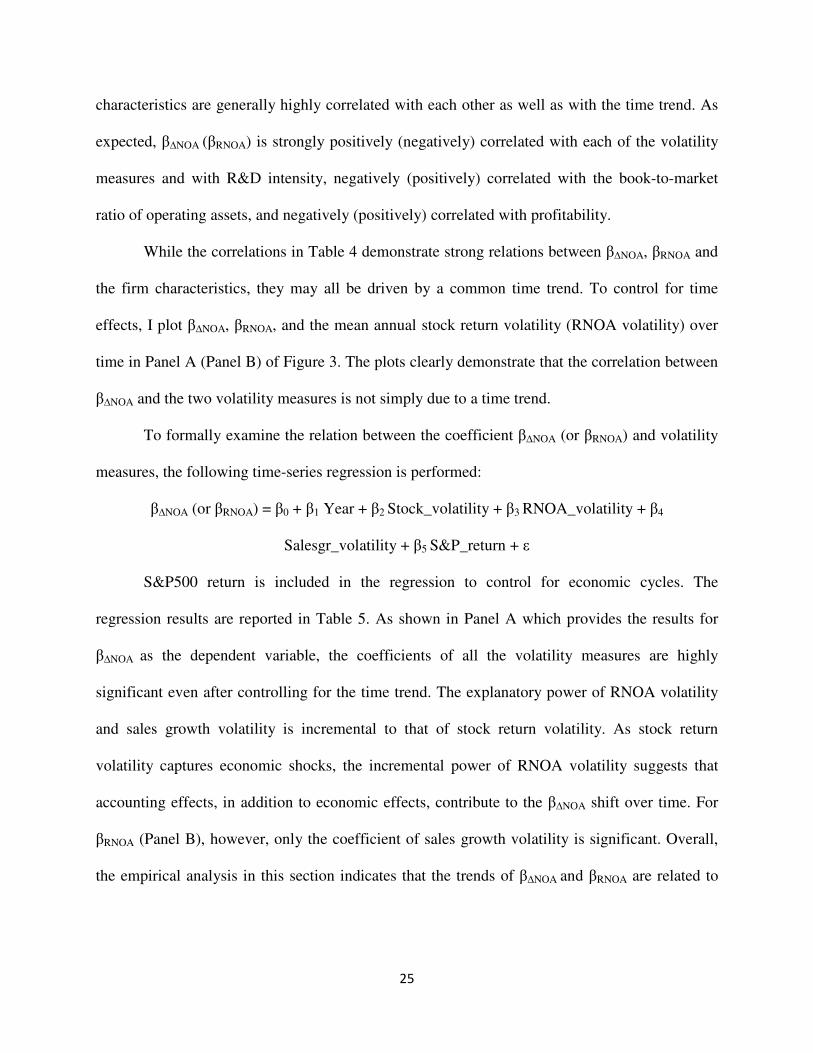
characteristics are generally highly correlated with each other as well as with the time trend. As
expected, β∆NOA (βRNOA) is strongly positively (negatively) correlated with each of the volatility
measures and with R&D intensity, negatively (positively) correlated with the book-to-market
ratio of operating assets, and negatively (positively) correlated with profitability.
While the correlations in Table 4 demonstrate strong relations between β∆NOA, βRNOA and
the firm characteristics, they may all be driven by a common time trend. To control for time
effects, I plot β∆NOA, βRNOA, and the mean annual stock return volatility (RNOA volatility) over
time in Panel A (Panel B) of Figure 3. The plots clearly demonstrate that the correlation between
β∆NOA and the two volatility measures is not simply due to a time trend.
To formally examine the relation between the coefficient β∆NOA (or βRNOA) and volatility
measures, the following time-series regression is performed:
β∆NOA (or βRNOA) = β0 + β1 Year + β2 Stock_volatility + β3 RNOA_volatility + β4
Salesgr_volatility + β5 S&P_return + ε
S&P500 return is included in the regression to control for economic cycles. The
regression results are reported in Table 5. As shown in Panel A which provides the results for
β∆NOA as the dependent variable, the coefficients of all the volatility measures are highly
significant even after controlling for the time trend. The explanatory power of RNOA volatility
and sales growth volatility is incremental to that of stock return volatility. As stock return
volatility captures economic shocks, the incremental power of RNOA volatility suggests that
accounting effects, in addition to economic effects, contribute to the β∆NOA shift over time. For
βRNOA (Panel B), however, only the coefficient of sales growth volatility is significant. Overall,
the empirical analysis in this section indicates that the trends of β∆NOA and βRNOA are related to
26
the factors laid out in Section 3.2.1, i.e., economic and accounting changes, changes in the
characters of the public firms, and the real option value effects.
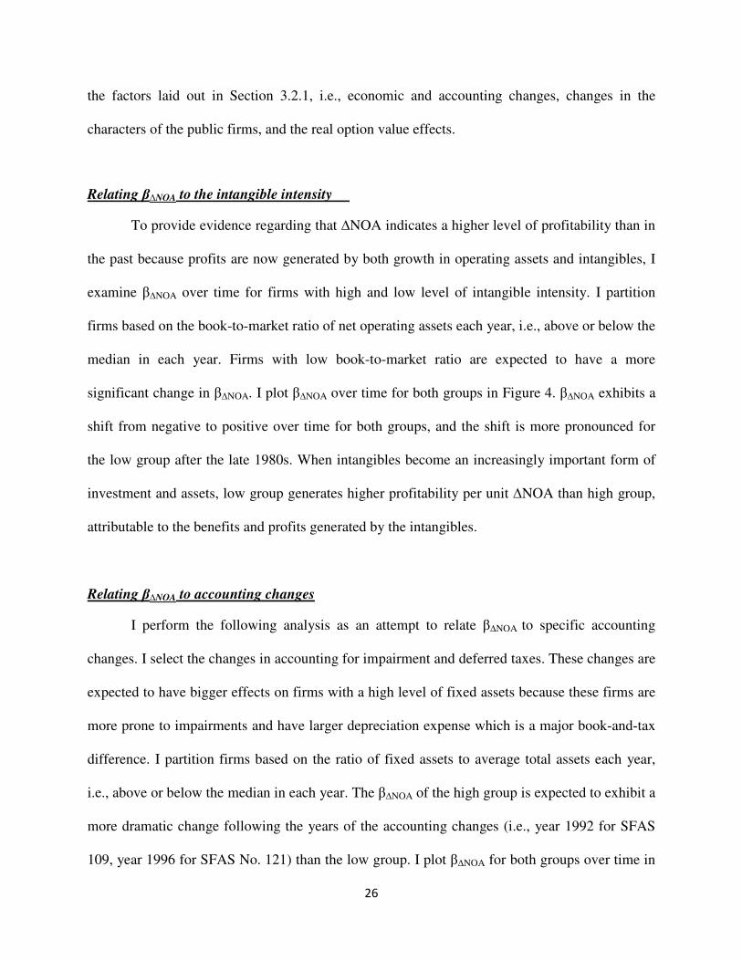
Relating β∆NOA to the intangible intensity
To provide evidence regarding that ∆NOA indicates a higher level of profitability than in
the past because profits are now generated by both growth in operating assets and intangibles, I
examine β∆NOA over time for firms with high and low level of intangible intensity. I partition
firms based on the book-to-market ratio of net operating assets each year, i.e., above or below the
median in each year. Firms with low book-to-market ratio are expected to have a more
significant change in β∆NOA. I plot β∆NOA over time for both groups in Figure 4. β∆NOA exhibits a
shift from negative to positive over time for both groups, and the shift is more pronounced for
the low group after the late 1980s. When intangibles become an increasingly important form of
investment and assets, low group generates higher profitability per unit ∆NOA than high group,
attributable to the benefits and profits generated by the intangibles.
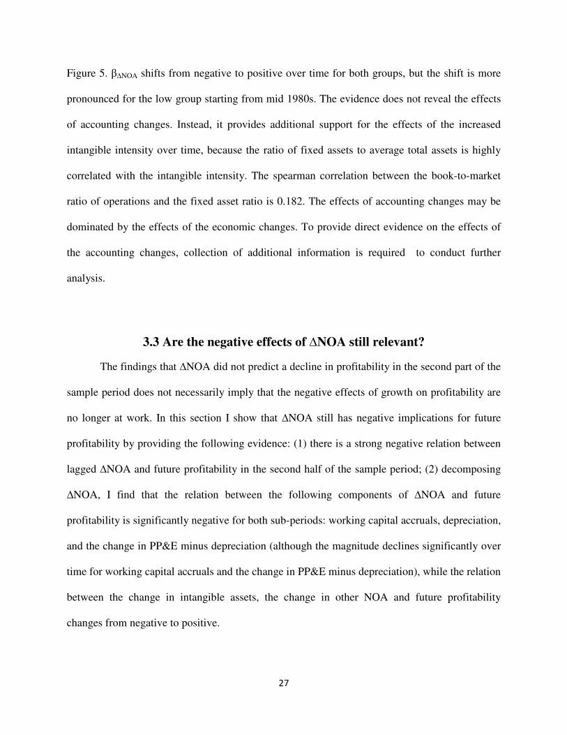
Relating β∆NOA to accounting changes
I perform the following analysis as an attempt to relate β∆NOA to specific accounting
changes. I select the changes in accounting for impairment and deferred taxes. These changes are
expected to have bigger effects on firms with a high level of fixed assets because these firms are
more prone to impairments and have larger depreciation expense which is a major book-and-tax
difference. I partition firms based on the ratio of fixed assets to average total assets each year,
i.e., above or below the median in each year. The β∆NOA of the high group is expected to exhibit a
more dramatic change following the years of the accounting changes (i.e., year 1992 for SFAS
109, year 1996 for SFAS No. 121) than the low group. I plot β∆NOA for both groups over time in
27
Figure 5. β∆NOA shifts from negative to positive over time for both groups, but the shift is more
pronounced for the low group starting from mid 1980s. The evidence does not reveal the effects
of accounting changes. Instead, it provides additional support for the effects of the increased
intangible intensity over time, because the ratio of fixed assets to average total assets is highly
correlated with the intangible intensity. The spearman correlation between the book-to-market
ratio of operations and the fixed asset ratio is 0.182. The effects of accounting changes may be
dominated by the effects of the economic changes. To provide direct evidence on the effects of
the accounting changes, collection of additional information is required to conduct further
analysis.
3.3 Are the negative effects of ∆NOA still relevant?
The findings that ∆NOA did not predict a decline in profitability in the second part of the
sample period does not necessarily imply that the negative effects of growth on profitability are
no longer at work. In this section I show that ∆NOA still has negative implications for future
profitability by providing the following evidence: (1) there is a strong negative relation between
lagged ∆NOA and future profitability in the second half of the sample period; (2) decomposing
∆NOA, I find that the relation between the following components of ∆NOA and future
profitability is significantly negative for both sub-periods: working capital accruals, depreciation,
and the change in PP&E minus depreciation (although the magnitude declines significantly over
time for working capital accruals and the change in PP&E minus depreciation), while the relation
between the change in intangible assets, the change in other NOA and future profitability
changes from negative to positive.
28
3.3.1 The negative relation between lagged ∆NOA and future profitability
The overall positive relation between ∆NOA and future profitability represents the net
effect of ∆NOA on future profitability, i.e., the negative effects are offset by the positive effects
due to the changes discussed in Section 3.2. To disentangle the negative effects from the
positive, I examine the incremental information of the one- and two-year lagged ∆NOA
regarding future profitability, after controlling for current ∆NOA.11
Because both the negative
and positive effects of ∆NOA on future profitability may persist for multiple years, finding that
the lagged ∆NOA terms are negatively related to future profitability in the second half of the
sample period would confirm the continuing presence of the negative effects of growth on
profitability.
Net operating assets essentially reflect the cumulative difference between operating
income and free cash flow (Hirshleifer et al. 2004), and this difference reverses over many future
years. The pattern of reversal depends on the transactions giving rise to the initial difference. For
example, when a firm inflates the balance sheet by over-capitalizing expenditures as fixed assets
(a positive ∆NOA), subsequent depreciation is increased by a constant amount each period over
the asset useful life. In contrast, overstating revenue by “stuffing the channels” would fully
reverse in the subsequent period unless the company re-engages in this earnings management
activity. Thus, ∆NOA may have negative implications for both near- and long-term profitability.
Similarly, the positive effects of ∆NOA on profitability may exhibit variable time
patterns. Examples of the positive effects of ∆NOA on future profitability include a decrease in
the tax valuation allowance due to an increase in expected earnings, or an impairment charge
triggered by a reduction in expected earnings (Rees et al. 1996, Li et al. 2011). Both examples
11
In unreported tests, I include three-year-lagged ∆NOA in the future profitability regression. The coefficient on the
three-year-lagged ∆NOA is not significant, and the coefficients of other explanatory variables, i.e., current ∆NOA,
one- and two-year lagged ∆NOA, do not change significantly.
29
suggest a positive correlation between ∆NOA and future profitability, with the time pattern of
the correlation depending on the pattern of related future earnings.
I assess the possible negative effects of ∆NOA on future profitability by including lagged
values of ∆NOA in the future profitability regression:
RNOAt+1 = β0 + β∆NOA ∆NOAt + β1 ∆NOAt-1 +β2 ∆NOAt-2 + βRNOA RNOAt + ε
The regression results are reported in Table 6. β∆NOA and βRNOA are generally similar to what are
reported in Table 2. The coefficients of one- and two-year lagged ∆NOA are insignificant in the
first sub-period, -0.0042 (t-stat=-0.9) and 0.0004 (t-stat=0.1), but are negative and significant in
the second period, -0.0275 (t-stat=-4.4) and -0.0131 (t-stat=-2.1).12
These results support the
hypothesis that the negative effects of growth on future profitability continue to exist in the
second period, but that the negative effects are dominated by the positive effects in the following
year.
3.3.2 The relation between components of ∆NOA and future profitability
I also examine whether any of the negative effects of ∆NOA on future profitability are
still relevant by decomposing ∆NOA into components. This allows for further examination of the
12
The finding that the delayed negative effects of growth on profitability are stronger in the second sample period is
consistent with managers opportunistically utilizing the balance-sheet approach. The shift from an income statement
to balance sheet approach makes book value more relevant, but it also provides managers with flexibility to
manipulate income in ways that take long periods to unwind. The balance sheet approach often incorporates
assumptions and estimates that are projected far into the future. Consider the following examples. Impairment
charges could reflect managers’ appropriate response to decreases in the assets’ ability to generate income (Smith
1993, Rees et al. 1996, Li et al. 2011), or they could be the result of managerial manipulation to improve future
earnings (Francis et al. 1996, Burgstahler et al. 2002). The latter results in a negative effect of growth on future
profitability, while the former indicates a positive effect. Studies have shown that after the implementation of SFAS
121 and SFAS 142, asset write-offs have become more strongly associated with “big bath” reporting behavior,
suggesting greater managerial discretion in reporting (Riedl 2004, Li et al. 2011). As another example, by
understating the valuation allowance for deferred tax assets (an increase in NOA), managers may be able to
overstate current income at the expense of future income (when the deferred tax asset expires unutilized). Similarly,
by understating expected compensation increases and therefore expected benefit payments under defined benefit
pension plans (an increase in NOA), managers may be able to postpone the related expenses for many years.
30
incremental relation of each component with future profitability. I examine the relation of the
components of ∆NOA with future profitability by running the following regression and report
the results in Table 7:
RNOAt+1 = β0 + β1 ∆WCt +β2 DepAcct + β3 Oth∆PP&Tt + β4 ∆Intant +β5 ∆OthNOAt + β6 RNOAt
+ ε
Working capital accruals, defined as the change in working capital minus depreciation
expense (as in Sloan 1996), is significantly negatively related to future profitability for both sub-
periods, -0.1419 (t-stat=-13.9) for the first and -0.0594 (t-stat=-2.4) for the second, although the
magnitude of the coefficient declines significantly over time (t-stat=3.0 for the change). The
coefficient of depreciation (negative sign) is -0.1122 (t-stat=-2.6) in the first period and -0.1897
(t-stat=-3.8) in the second, and the change is marginally significant (t-stat=-1.2). The coefficient
of the change in PP&E minus depreciation becomes less negative over time: -0.1044 (t-stat=-
12.0) in the first period and -0.0317 (t-stat=-2.4) in the second, and the change is significant (t-
stat=4.6). The changes in the coefficients are consistent with the effects of intangibles: growth in
working capital accruals and fixed assets (hence less depreciation) is associated with a higher
level of profitability. At the same time, the coefficient of the change in intangible assets shifts
from -0.0496 (t-stat=-1.8) in the first period to 0.0010 (t-stat=0.1) in the second, and the increase
is marginally significant (t-stat=1.6). The coefficient of the other ∆NOA changes significantly
from -0.1073 (t-stat=-14.5) to 0.0493 (t-stat=-3.5). The results provide further support for the
inference that the negative implications of ∆NOA for future profitability are still in force. The
positive effects grow stronger over time and now dominate the negative effects.
31
4. Implications for the accrual anomaly
The changes in the relation between ∆NOA and future profitability have important
implications for the accrual anomaly—i.e., the negative relation between ∆NOA and future stock
returns. The prevailing explanation for the anomaly in the literature is that ∆NOA implies a
reduction in future profitability, and investors fail to fully appreciate this negative relation; the
mispricing is corrected when future earnings are announced. In support of this explanation,
several studies (e.g., Fairfield et al. 2003, Fama and French 2006) document that ∆NOA is
negatively related to future profitability after controlling for current profitability. However, the
positive relation between ∆NOA and future profitability documented in this study implies that
the anomaly should no longer exist. Therefore, I proceed to re-examine the relation between
∆NOA and future stock returns.
4.1 The accrual anomaly over time
Since Sloan (1996) first documented the accrual anomaly, the literature has generally
found it to be robust. However, a few recent studies (Richardson et al. 2010, Wu et al. 2010,
Green et al. 2011) report that forming investment strategies based on ∆NOA does not generate
significant abnormal return in the mid 2000s. Yet Green et al. (2011) notes that “although hedge
returns to Sloan’s (1996) accrual anomaly are not currently positive on average, they may not
always remain so”. Similarly, Wu et al. (2010) suggests that the deterioration of the accrual
anomaly in recent years reflects its counter-cyclical nature, and the accruals effect is likely to
mean-revert in the near future. Moreover, the profitability of an investment strategy depends on
business conditions, type and magnitude of profit opportunities in other strategies, and many
other known or unknown factors that may change over time. For example, Richardson et al.
32
(2010) reports that the post-earnings-announcement drift was weaker for a few years until 2002,
generated marginally positive returns for the years 2003-2005, and became insignificant again in
recent years. They note “the possibility that time varying expected returns could explain the
attenuation in the return profile of the ∆NOA and SUE characteristic portfolios”.
I examine the accrual anomaly over the period 1967-2010 (stock returns through April
2012), extending the sample periods employed in prior studies. To assure robustness, I use
Fama-MacBeth regression, a portfolio approach, and a Fama-French factor analysis. Table 8
reports the results of the following regression:
Rett+1 = β0 + β1 ∆NOAt + β2 RNOAt + β3 RNOAt-1 + β4 Sizet + β5 BTMt + β6 Betat
+ β7 Idio_Volatt + β8 Rett + ε
Consistent with prior studies, ∆NOA negatively predicts future stock returns. In addition, the
coefficient of size is negative and significant, the coefficients of book-to-market and momentum
(Rett) are positive and significant, the coefficient of market beta is insignificant, and the
coefficient of idiosyncratic volatility is negative rather than positive (see, e.g., Ang et al. 2006).
The annual ∆NOA coefficients to predict future returns are plotted in Figure 6. For the
majority of the sample years, the ∆NOA coefficient is negative. Similar to the findings in prior
studies, the accrual anomaly weakens during the mid 2000s; however, the negative relation
between ∆NOA and future stock returns resumes after 2006 with a large magnitude. In addition,
for several years during the 1970s, the anomaly was insignificant but, similar to the pattern
observed in the late 2000s, those years were followed by a strong and consistent performance.
Visual examination of the time-series pattern suggests that while the magnitude of the coefficient
may have declined during the second half of the sample period, it remains consistently negative.
The last two sets of regression results reported in Table 8 confirm that ∆NOA’s ability to predict
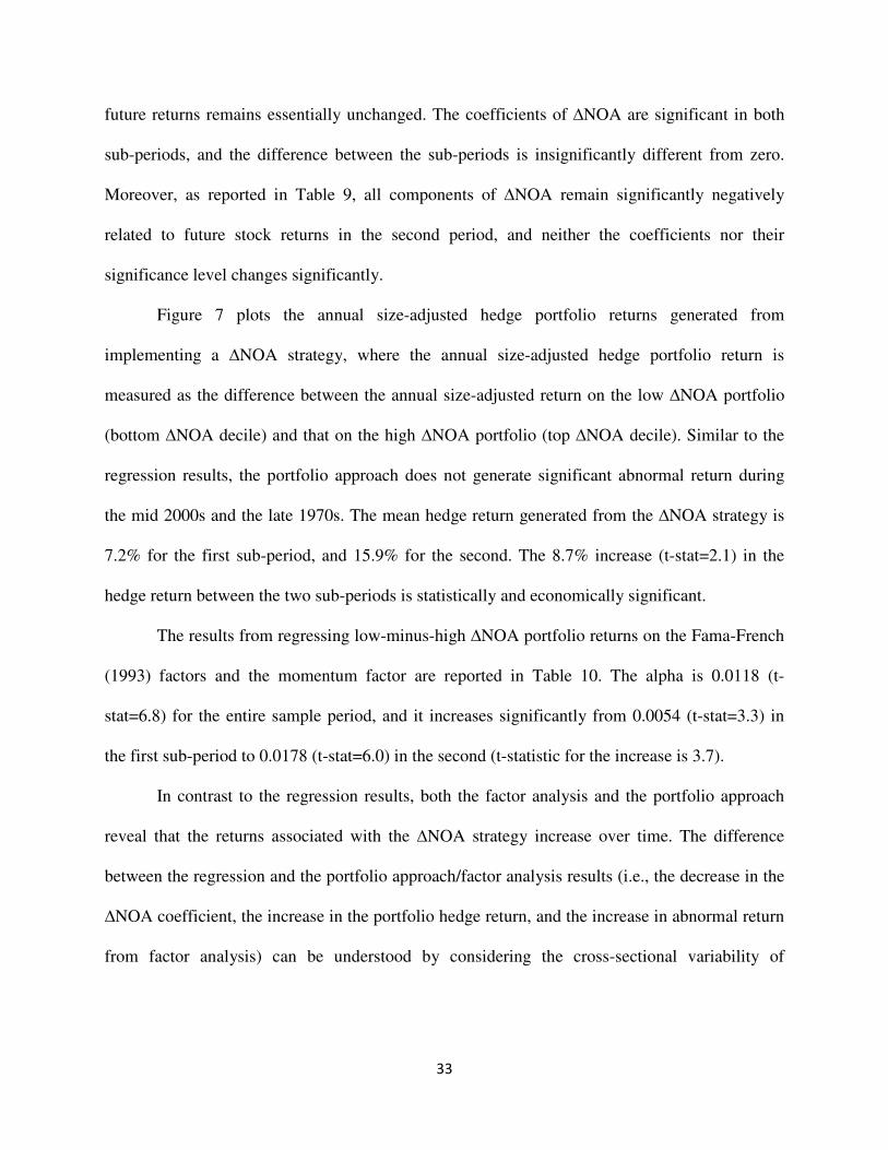
33
future returns remains essentially unchanged. The coefficients of ∆NOA are significant in both
sub-periods, and the difference between the sub-periods is insignificantly different from zero.
Moreover, as reported in Table 9, all components of ∆NOA remain significantly negatively
related to future stock returns in the second period, and neither the coefficients nor their
significance level changes significantly.
Figure 7 plots the annual size-adjusted hedge portfolio returns generated from
implementing a ∆NOA strategy, where the annual size-adjusted hedge portfolio return is
measured as the difference between the annual size-adjusted return on the low ∆NOA portfolio
(bottom ∆NOA decile) and that on the high ∆NOA portfolio (top ∆NOA decile). Similar to the
regression results, the portfolio approach does not generate significant abnormal return during
the mid 2000s and the late 1970s. The mean hedge return generated from the ∆NOA strategy is
7.2% for the first sub-period, and 15.9% for the second. The 8.7% increase (t-stat=2.1) in the
hedge return between the two sub-periods is statistically and economically significant.
The results from regressing low-minus-high ∆NOA portfolio returns on the Fama-French
(1993) factors and the momentum factor are reported in Table 10. The alpha is 0.0118 (t-
stat=6.8) for the entire sample period, and it increases significantly from 0.0054 (t-stat=3.3) in
the first sub-period to 0.0178 (t-stat=6.0) in the second (t-statistic for the increase is 3.7).
In contrast to the regression results, both the factor analysis and the portfolio approach
reveal that the returns associated with the ∆NOA strategy increase over time. The difference
between the regression and the portfolio approach/factor analysis results (i.e., the decrease in the
∆NOA coefficient, the increase in the portfolio hedge return, and the increase in abnormal return
from factor analysis) can be understood by considering the cross-sectional variability of
34
∆NOA.13
The annual standard deviation of ∆NOA increases from 15.6% in the first sub-period to
28.7% in the second, and the increase is significant (t-stat = 7.4).
4.2 Existing Explanations for the accrual anomaly
Having shown that the accrual anomaly still exists, I next study the explanations for the
anomaly offered in prior research. Two alternative explanations for the negative relation between
∆NOA and future stock returns have been offered in the literature.
The first explanation suggests that ∆NOA is negatively related to risk, so the return
predictability of ∆NOA is not anomalous. Economic theory suggests that a decline in discount
rates should lead to both an increase in the firm’s operating assets (i.e., more projects have
positive net present value) and a decline in realized stock returns (Fama and French 1995 &
1996, Zhang 2007, Wu et al. 2010). Penman and Zhu (2012) takes the view that the observed
“anomalous” returns associated with working capital accruals are consistent with rational pricing
because working capital accruals forecast forward earning yields and growth in the same
direction in which they forecast returns. The Fama-French factor analysis (Table 10) provides
evidence supporting the possible role of risk. High-minus-low, small-minus-big, and the
momentum factors all load positively in explaining the low-minus-high ∆NOA portfolio return.
The loading of the market factor is negative, indicating that the ∆NOA strategy is counter-
cyclical.
13
To illustrate how the increase in the variability of ∆NOA can explain the difference between the regression and
portfolio results, consider the following example. Case (a): mean ∆NOA is equal to -1 for the bottom decile and 1
for the top decile, and the size-adjusted portfolio return is 10% for the bottom decile and -10% for the top decile.
Under this setting, the hedge return is 20%, and the ∆NOA coefficient when regressing future stock returns on
∆NOA is 10. Case (b): mean ∆NOA is equal to -10 for the bottom decile and 10 for the top decile, and the size-
adjusted stock portfolio return is 20% for the bottom decile and -20% for the top decile. Under this setting, the
hedge return is 40% and the ∆NOA coefficient is 2. Note that the hedge return is larger in case (b) while the ∆NOA
coefficient is smaller, and this difference is due to the increase in the cross-sectional variability of ∆NOA.
35
While the results of the Fama-French factor analysis suggest that exposure to risk factors
contributes to the negative relation between ∆NOA and future stock returns, risk is unlikely to
fully explain the anomaly given the significant “intercept”. Hirshleifer et al. (2012) shows that “it
is the accrual characteristic rather than the accrual factor loading that predicts returns”, which is
consistent with the behavioral/mispricing hypothesis. Moreover, the consistency of the anomaly
throughout the sample period (see Figures 6 and 7), the relatively small magnitude of negative
abnormal returns when the strategy does not work, and the fact that strategy performs well in
recession years,14
suggest that risk-pricing is unlikely to fully explain the negative relation
between ∆NOA and future stock returns.
The second explanation for the anomaly is that ∆NOA predicts a decline in future
profitability and investors fail to fully appreciate this negative relation. Stock prices fully
impound the information when future profitability is announced. However, this explanation
cannot explain the persistence of the anomaly because ∆NOA does not predict a reduction in the
next year’s profitability during the last twenty years as this study shows.
4.3 Hypothesized Explanation for the accrual anomaly
In this section I conjecture and show that the accrual anomaly is associated with the
divergence between the market reaction to ∆NOA and the future profitability implications of
∆NOA throughout the sample period. Investors are always over-optimistic about the profitability
implications of ∆NOA, i.e., in the first half of the sample (1967-1988), investors do not fully
react to the negative effects of growth on profitability, and in the second half (1989-2010), they
14
Lakonishok et al. (1994) assesses the risk-based explanation to the value/glamour strategy based on the argument
that value stocks would be fundamentally riskier if they underperform glamour stocks in “bad” states of the world.
36
appear to over-emphasize the positive implications of ∆NOA for future profitability. I also rule
out the possibility that in recent years the accrual anomaly is caused by market mispricing of the
past (rather than current) ∆NOA.
4.3.1 Divergence between the market pricing and the profitability implications of
∆NOA
My empirical results with respect to the first sub-period are consistent with the prevailing
explanation for the accrual anomaly: ∆NOA is negatively related to future profitability and
investors do not fully react to this negative relation (e.g., Sloan 1996, Xie 2001, Fairfield et al.
2003). However, in the second sub-period, I find that ∆NOA is positively related to future
profitability, and yet the accrual anomaly persists. I conjecture that the persistence of the
anomaly in the second sub-period is related to investors’ excessive focus on the positive
information in ∆NOA. The positive information in ∆NOA results from the economic changes
and the accounting principles shifting toward a balance sheet/fair value approach. In their survey
paper, Dichev et al. (2012) reports that CFOs express concerns that “over-emphasis of the fair
value approach is misguided”. Investors’ over-extrapolation of certain information items is the
alternative explanation for several stock market anomalies: investors initially overreact to the
information item, and the stock return predictability of that item reflects the future reversal of the
overreaction. For example, the value/growth anomaly is argued to be attributable to investors’
overreaction to the past performance of glamor firms (e.g., De Bondt and Thaler 1985,
Lakonishok et al. 1994). To summarize, I conjecture that the accrual anomaly is associated with
the divergence between the market reaction to ∆NOA and the future profitability implications of
∆NOA throughout the sample period.
37
I examine this conjecture by comparing the market pricing of ∆NOA with the
profitability implications of ∆NOA. The market pricing of ∆NOA is assessed by regressing
contemporaneous stock returns on ∆NOA and control variables:
Rett = β0 + β1 ∆NOAt + β2 ∆NOAt-1 + β3 ∆NOAt-2 + β4 RNOAt + β5 RNOAt-1
+ β6 Sizet-1 + β7 BTMt-1 + β8 Betat-1 + β9 Idio_Volatt-1 + β10 Rett-1 + ε
The regression results are reported in Table 11. During the first sub-period investors’
reaction to ∆NOA is negative, but it changes to be strongly positive in the second sub-period (t-
statistic=7.1 for the change). Table 12 shows that the changes in investors’ response to all the
components of ∆NOA are similar.
To compare and contrast the market reaction to ∆NOA with the future profitability
implications of ∆NOA, I plot in Figure 8 the time-series pattern of the ∆NOA coefficients from
the contemporaneous stock return regression (Table 11) and β∆NOA from the profitability
regression (Table 2). As the scale of the ∆NOA coefficients from the contemporaneous stock
return regression and β∆NOA are not comparable, I “standardize” each coefficient series by
dividing the coefficients by their time-series standard deviation. The variability of the
standardized coefficients is comparable across the two series. In other words, the magnitude of
changes in the standardized coefficients is comparable across the two series.
From the mid 1960s through the early 1980s, β∆NOA is significantly negative and
relatively stable, indicating that ∆NOA has strong negative implications for future profitability.
β∆NOA slopes upward in the mid 1980s, and becomes positive in the mid 1990s. It fluctuates
mainly in the positive range from the late 1990s onwards, suggesting that ∆NOA has net positive
implications for future profitability during this period. In contrast, the ∆NOA coefficient from
the contemporaneous stock returns regression slopes upward from the mid 1970s, becomes
38
positive in the early 1980s, and stabilizes in the positive range after the late 1980s. It indicates
that investors start to react positively to ∆NOA in the early 1980s, and their positive reaction has
remained relatively stable since then.
A comparison of β∆NOA and the ∆NOA coefficient from the contemporaneous stock
returns regression suggests the following with respect to the persistence of the accrual anomaly.
During the period 1966-1987, ∆NOA has strong negative implications for future profitability but
investors fail to fully react to those implications. However, starting from the late 1980s, the
market seems to overprice the positive implications of ∆NOA relative to the realization of future
profitability. The decline of the anomaly in the mid 2000s is in a period when investors’ reaction
to ∆NOA and the profitability implications of ∆NOA converge. The resumption of the anomaly
in the late 2000s can be explained by a divergence between market expectations and profitability
realizations, i.e., investors continue to react positively to ∆NOA while ∆NOA does not positively
predict future profitability during that short period of time. Considering that market pricing of
∆NOA has been stable over the past twenty years, it is the profitability implications of ∆NOA
that shift over time and diverge from market pricing.
4.3.2 The possible role of lagged NOA in explaining the accrual anomaly
In Section 3.3.1, lagged values of ∆NOA are shown to be negatively related to future
profitability. Because ∆NOA and lagged ∆NOA are highly correlated (average cross-sectional
Pearson (Spearman) correlation coefficient between ∆NOA and lagged ∆NOA over the sample
years is 0.24 (0.30)), it is possible that the negative relation between ∆NOA and future stock
return in the second sub-period is due to the market mispricing of lagged ∆NOA. I next examine
39
whether the persistence of the accrual anomaly is related to the market mispricing of lagged
∆NOA by including one- and two-year lagged ∆NOA in the profitability regression:
Rett+1 = β0 + β1 ∆NOAt + β2 ∆NOAt-1 + β3 ∆NOAt-2 + β4 RNOAt + β5 RNOAt-1 + β6 Sizet
+ β7 BTMt + β8 Betat + β9 Idio_Volatt + β10 Rett + ε
The results, reported in Table 13, show that the ∆NOA coefficient is not significantly
altered by the inclusion of the lagged ∆NOA terms, suggesting that the delayed effects of ∆NOA
do not explain the persistence of the accrual anomaly. One-year lagged ∆NOA negatively
predicts stock returns throughout the sample period, and the coefficient of the two-year lagged
∆NOA is negative and significant only in the last twenty years.
40
5. Robustness Tests
Alternative measures of ∆NOA and RNOA
To be comparable with existing studies and remove the possibility that the results are
driven by the relation between cash and future profitability, I repeat all the analysis with the
alternative measures of ∆NOA and RNOA that exclude cash and the related interest income. Net
operating assets are measured as total assets minus cash, short-term investment, and non-debt
liabilities; NOPAT, the numerator of RNOA, is calculated as net income before extraordinary
items and after minority interest, minus after-tax special items, plus after-tax interest expense,
minus after-tax interest income, plus minority interest in income. All the major results hold for
the alternative measures. Table 14 reports the results from examining the relation between
growth and future profitability with the alternative measures. The results are consistent with the
primary analysis, i.e., ∆NOA changes from negatively to positively predicting future profitability
over time.
Excluding merger and acquisition cases
Assets acquired and liabilities assumed in a business combination may have different
implications for future profitability from existing resources. To remove the possible effects of
business combinations, I repeat the major analysis excluding observations with significant
business combinations. Firms having either a change of intangible or cash paid for acquisitions
greater than 5% of average total assets are considered as having significant business
combinations. The major results hold after excluding significant business combination cases, as
reported in Table 15.
41
Positive versus negative ∆NOA
Positive and negative ∆NOA may have different implications for future profitability. For
example, Barth et al. (1998) shows that pricing multiples and the incremental explanatory power
of equity book value (net income) increase (decrease) as financial health decreases, because
liquidation values and probability of default affect equity values. To ensure that the results are
not driven by the negative growth cases, I allow different coefficients for positive and negative
growth and report the results in Table 16. For firms with positive ∆NOA, β∆NOA is -0.1183 (t-
stat=-22.5) for the first sub-period, and increases significantly to -0.0659 (t-stat=-8.3) in the
second. For firms with negative ∆NOA, β∆NOA changes from -0.0341 (t-stat=-2.2) in the first sub-
period to 0.3465 (t-stat=7.4) in the second, and the change is significant (t-stat=7.7). Firms with
negative ∆NOA are likely to have more intangibles.
42
6. Conclusion and limitations
Growth in net operating assets has both negative and positive implications for future
profitability. Positive implications are expected to grow stronger over time due to economic and
accounting changes. From the valuation perspective, future profitability can be expressed as a
weighted average of current profitability and growth in net operating assets, with the weights
depending on the persistence of current earnings. Prior research finds a decline in earnings
persistence and a shift of value relevance from earnings to book value over time. This study
reexamines the ability of growth in net operating assets and current profitability to predict future
profitability. Contrary to the understanding of an overall negative relation between ∆NOA and
future profitability, this study finds that the relation has been positive since the mid 1990s. The
∆NOA coefficient from the future profitability regression (β∆NOA) is negative in the first half of
the sample period (1967-1988), but slopes upward in the late 1980s, and becomes positive after
the mid 1990s.
The shift in the relation between ∆NOA and future profitability is related to the increase
in book value’s ability to predict future profitability and the increased intangible intensity. β∆NOA
is strongly correlated with stock return volatility, earnings volatility, special items, R&D
intensity, and other volatility-related characteristics. The increase in earnings volatility and the
improvement in the relevance of book value are attributable to economic and accounting
changes, changing characteristics of public firms, and the increased importance of real options.
Moreover, as the intangible intensity increases over time, ∆NOA is associated with a higher level
of profitability because the profits now are contributed by both ∆NOA and intangibles.
This paper further shows that the negative effects of ∆NOA on future profitability
continue to exist in the second half of the sample period, but the negative effects are dominated
43
by the positive effects of ∆NOA in the following year. Decomposing ∆NOA reveals that
working capital accruals, depreciation, and the change in PP&E minus depreciation remain
negatively related to future profitability throughout the sample period. In contrast, the relation
between the change in intangible assets, the other ∆NOA and future profitability shifts from
negative to positive.
The shift in the relation between ∆NOA and future profitability has important
implications for the accrual anomaly—i.e., the negative relation between ∆NOA and future stock
returns. The prevailing explanation for the anomaly is that ∆NOA implies a reduction in future
profitability, which investors fail to fully appreciate; the mispricing is corrected when future
earnings are announced. The change in the future profitability-∆NOA relation documented in
this study implies that the anomaly should no longer exist. Indeed, several recent studies
document that the accrual anomaly weakens during the mid 2000s. I examine the accrual
anomaly over the period of 1967 to 2010, and find evidence that the accrual anomaly still exists.
Specifically, the results show that the anomaly resumes after 2006, and in the 1970s there was a
short period during which the anomaly was insignificant and exhibited a similar pattern as that
found in the mid 2000s. When the entire sample period is divided into two equal length sub-
periods, the change in the magnitude of the anomaly between the two sub-periods is
insignificant. Additionally, all components of ∆NOA are significantly related to future stock
returns, and the strength of these relations does not change during the sample period.
Considering the change in the future profitability-∆NOA relation, what could explain the
persistence of the accrual anomaly throughout the sample period? Risk may contribute to the
persistence of the anomaly over time, but it seems unlikely to fully explain it. I conjecture and
show that the anomaly is related to the divergence between the market pricing and profitability
44
implications of ∆NOA throughout the sample period. Specifically, investors do not fully react to
the negative profitability implications of ∆NOA through the late 1980s, and they seem to over-
emphasize the positive implications of ∆NOA afterwards. The decline of the anomaly in the mid
2000s is shown to be associated with the convergence of investors’ expectations and the
realization of the future profitability. The anomaly resumes in the late 2000s as the divergence
emerges again: investors continue to react positively to ∆NOA while ∆NOA becomes
insignificantly related to future profitability. Over the last twenty years, investors’ reaction to
∆NOA has been relatively stable, and it is the profitability implications of ∆NOA that shift over
time and cause the divergence.
45
References
Amir, E., M. Kirshenheiter, and K. Willard. 1997. The Valuation of Deferred Taxes.
Contemporary Accounting Research 14: 597-622.
Amir, E., M. Kirschenheiter, and K. Willard. 2001. The aggregation and valuation of deferred
taxes. Review of Accounting Studies 6: 275–297.
Amir, E., and B. Lev. 1996. Value-Relevance of NonFinancial Information: The Wireless
Communications Industry. Journal of Accounting and Economics 22: 3–30.
Amir, E., and T. Sougiannis. 1999. Analysts’ Interpretation and Investors’ Valuation of Tax
Carry-Forwards. Contemporary Accounting Research 16: 1-33.
Ang, A., R. J. Hodrick, Y. Xing, and X. Zhang. 2006. The Cross-Section of Volatility and
Expected Returns. Journal of Finance 61: 259-299.
Ayers, B. 1998. Deferred Tax Accounting Under SFAS No.109: An Empirical Investigation of
its Incremental Value-Relevance Relative to APB No.11. The Accounting Review 73:
195–212.
Baber, W. R., S. Kang, and Y. Li. 2011. Modeling Discretionary Accrual Reversal and the
Balance Sheet as an Earnings Management Constraint. The Accounting Review 86:
1189–212.
Barth, M. E. 1991. Relative Measurement Errors Among Alternative Pension Asset and
Liability Measures. The Accounting Review 66: 433–463.
Barth, M. E. 1994. Fair Value Accounting: Evidence from Investment Securities and the
Market Valuation of Banks. The Accounting Review 69: 1-25.
Barth, M. E. 2006. Including Estimates of the Future in Today’s Financial Statements.
Accounting Horizons 20: 271-285.
Barth, M. E., W. H. Beaver, and W. R. Landsman. 1992. The Market Valuation Implications of
Net Periodic Pension Cost Components. Journal of Accounting and Economics 15: 27–
62.
Barth, M. E., W. H. Beaver, and W. R. Landsman. 1993. A Structural Analysis of Pension
Disclosures Under SFAS 87 and their Relation to Share Prices. Financial Analysts
Journal 49: 18–26.
Barth, M. E., W. H. Beaver, and W. R. Landsman. 1996. Value-Relevance of Banks’ Fair Value
Disclosures Under SFAS No. 107. The Accounting Review 71: 513-537.
Barth, M. E., W. H. Beaver, and W. R. Landsman. 1998. Relative Valuation Roles of Equity
Book Value and Net Income as a Function of Financial Health. Journal of Accounting
and Economics 25: 1–34.
Barth, M. E., W. H. Beaver, and W. R. Landsman. 2001. The Relevance of Value Relevance
Research for Financial Accounting Standard Setting: Another View. Journal of
Accounting and Economics 31: 77–104.
46
Barth, M. E., W. R. Landsman, and J. M. Wahlen. 1995. Fair Value Accounting: Effects on
Banks’ Earnings Volatility, Regulatory Capital, and Value of Contractual Cash Flows.
Journal of Banking and Finance 19: 577-605.
Barton, J., and P. J. Simko. 2002. The Balance Sheet as an Earnings Management Constraint.
The Accounting Review 77: 1-27.
Bartov, E., F. W. Lindahl, and W. E. Ricks. 1998. Stock Price Behavior around Announcements
of Write-Offs. Review of Accounting Studies 3: 327-346.
Basu, S. 1997. The Conservatism Principle and the Asymmetric Timeliness of Earnings.
Journal of Accounting and Economics 24: 3–37.
Black, E., T. Carnes, and V. J. Richardson. 2000. The Value Relevance of Multiple Occurrences
of Nonrecurring Items. Review of Quantitative Finance and Accounting 15: 391-411
Burgstahler, D., and I. Dichev. 1997. Earnings Management to Avoid Earnings Decreases and
Losses. Journal of Accounting and Economics 24: 99-126.
Burgstahler, D., J. Jiambalvo, and T. Shevlin. 2002. Do Stock Prices Reflect the Implications of
Special Items for Future Earnings?. Journal of Accounting Research 40: 585–612.
Campbell, J. Y., X. Lettau, B.G. Malkiel, and Y. Xu. 2001. Have Individual Stocks Become
More Volatile? An Exploration of Idiosyncratic Risk. Journal of Finance 56: 1-43.
Chan, K., L. Chan, N. Jegadeesh, and J. Lakonishok. 2006. Earnings Quality and Stock
Returns. Journal of Business 79: 1041-1082.
Collins, D., G. Gong, and P. Hribar. 2003. Investor Sophistication and the Mispricing of
Accruals. Review of Accounting Studies 8: 251–276.
Collins, D., and P. Hribar. 2000. Earnings-Based and Accruals-Based Market Anomalies: One
Effect or Two? Journal of Accounting and Economics 29: 101–123.
Collins, D., E. Maydew, and I. Weiss. 1997. Changes in the Value Relevance of Earnings and
Book Values Over the Past 40 Years. Journal of Accounting and Economics 24: 39–68.
Collins, D., M. Pincus, and H. Xie. 1999. Equity Valuation and Negative Earnings: The Role of
Book Value of Equity. The Accounting Review 74: 29–61.
Core, J., W. Guay, and R. Verdi. 2008. Is Accruals Quality a Priced Risk Factor? Journal of
Accounting and Economics 46: 2-22.
Comin, D., and S. Mulani. 2005. A Theory of Growth and Volatility at the Aggregate and Firm
Level." NBER Working Paper no. 11503. Cambridge, MA: National Bureau of Economic
Research.
Comin, D., and S. Mulani. 2006. Diverging Trends in Aggregate and Firm Volatility. Review of
Economics and Statistics 88: 374-383.
Comin, D., and T. Philippon. 2005. The Rise in Firm-Level Volatility: Causes and
Consequences. NBER Macroeconomics Annual, M. Gertler and K. Orgoff, eds. MIT
Press.
De Bondt, F. M., Werner, and R. H. Thaler. 1985. Does the Stock Market Overreact? Journal
of Finance 40 (1985): 793-805.
47
De Bondt, F. M., Werner, and R. H. Thaler. 1987. Further Evidence on Investor Overreaction
and Stock Market Seasonality. Journal of Finance 42: 557-581.
Dechow, P. M. 1994. Accounting Earnings and Cash Flows as Measures of Firm Performance:
The Role of Accounting Accruals. Journal of Accounting and Economics 18: 3–42.
Dechow, P. M., and I. D. Dichev. 2002. The Quality of Accruals and Earnings: The Role of
Accrual Estimation Errors. The Accounting Review 77: 35–59.
Dechow, P. M., A. P. Sweeney, J. H. Kim, and R. G. Sloan. 2012. Detecting Earnings
Management: A New Approach. Journal of Accounting Research 50: 275-334.
Dechow, P. M., and W. Ge. 2006. The Persistence of Earnings and Cash Flows and the Role of
Special Items: Implications for the Accrual Anomaly. Review of Accounting Studies 11:
253–296.
Dechow, P. M., W. Ge, and C. Schrand. 2010. Understanding Earnings Quality: A Review of
the Proxies, Their Determinants and Their Consequences. Journal of Accounting and
Economics 50: 344–401.
Dechow, P. M., L. A. Myers, and C. SHAKESPEARE. 2010. Fair Value Accounting and Gains
from Asset Securitizations: A Convenient Earnings Management Tool with
Compensation Side-Benefits. Journal of Accounting and Economics 49: 2-25.
Dechow, P. M., R. G. Sloan, and A. P. Sweeny. 1995. Detecting Earnings Management. The
Accounting Review 70: 193–225.
Dechow, P. M., R. G. Sloan. 1991. Executive Incentives and the Horizon Problem: An
Empirical Investigation. Journal of Accounting and Economics 14: 51-89.
Dechow, P. M., R. G. Sloan. 1997. Returns to Contrarian Investments: Tests of the Naive
Expectations Hypothesis. Journal of Financial Economics 43: 3-27.
Desai, H., S. Rajgopal, and M. Venkatachalam. 2004. Value-Glamour and Accruals Mispricing:
One Anomaly or Two? The Accounting Review 79: 355–85.
Dichev, I.D. 2003. Discussion of the Differential Persistence of Accruals and Cash Flows for
Future Operating Income Versus Future Profitability. Review of Accounting Studies 8:
245-250.
Dichev, I., J. Graha, and S. Rajgopal. 2012. Earnings Quality: Evidence from the Field.
Working Paper, Emory University.
Dichev, I., and V. Tang. 2008. Matching and the Changing Properties of Accounting Earnings
Over the Last 40 Years. The Accounting Review 83: 1425–1460.
Dichev, I., and V. Tang. 2009. Earnings Volatility and Earnings Predictability. Journal of
Accounting and Economics 47: 160–181.
Donelson, D. C., R. Jennings, and J. McInnis. 2011. Changes over time in the revenue-expense
relation: Accounting or economics? The Accounting Review 86: 945-974.
Elliot, J., and D. Hanna. 1996. Repeated Accounting Write-Offs and the Information Content of
Earnings. Journal of Accounting Research 34: 135–155.
48
Elliott, J., and W. Shaw. 1988. Unusual charges as accounting procedures to manage
perceptions. Journal of Accounting Research 26: 91-126.
Fairfield, P. M., S. Whisenant, and T. L. Yohn. 2003a. Accrued Earnings and Growth:
Implications for Future Profitability and Market Mispricing. The Accounting Review 78:
353–71.
Fairfield, P. M., S. Whisenant, and T. L. Yohn. 2003b. The Differential Persistence of Accruals
and Cash Flows for Future Operating Income versus Future Profitability. Review of
Accounting Studies 8: 221-243.
Fama, E., and K. R. French. 1993. Common Risk Factors in the Returns on Stocks and Bonds.
Journal of Financial Economics 33: 3–56.
Fama, E., and K. R. French. 1995. Size and Book-to-Market Factors in Earnings and Returns.
Journal of Finance 50: 131–55.
Fama, E., and K. R. French. 1996. Multifactor Explanations of Asset Pricing Anomalies.
Journal of Finance 51: 55–84.
Fama, E., and K. R. French. 1997. Industry Costs of Equity. Journal of Financial Economics
43: 153-193.
Fama, E., and K. R. French. 2001a. Disappearing Dividends: Changing Firm Characteristics or
Lower Propensity to Pay? Journal of Financial Economics 60: 3–43.
Fama, E., and K. R. French. 2001b. Newly Listed Firms: Fundamentals, Survival Rates, and
Returns. Center for Research in Security Prices. Working paper No. 530, University of
Chicago, Graduate School of Business.
Fama, E., and K. R. French. 2002. The Equity Premium. Journal of Finance 57: 637–59.
Fama, E., and K. R. French. 2006. Profitability, Investment, and Average Returns. Journal of
Financial Economics 82: 491–518.
Fama, E., and K. R. French. 2008. Dissecting Anomalies. Journal of Finance 63: 1653–78.
Fama, E., and J. Macbeth. 1973. Risk, Return, and Equilibrium: Empirical Tests. Journal of
Political Economy 81: 607–36.
Feltham, G. A., and J. A. Ohlson. 1995. Valuation and Clean Surplus Accounting for Operating
and Financial Activities. Contemporary Accounting Research 11: 689–731.
Francis, J., D. Hanna, and L. Vincent. 1996. Causes and Effects of Discretionary Asset Write-
Offs. Journal of Accounting Research 34: 117–134.
Francis, J., R. Lafond, P. Olsson, and K. Schipper. 2005. The Market Pricing of Accruals
Quality. Journal of Accounting and Economics 39: 295–327.
Francis, J., and K. Schipper. 1999. Have Financial Statements Lost Their Relevance? Journal
of Accounting Research 37: 319–352.
Givoly, D., and C. Hayn. 2000. The Changing Time-Series Properties of Earnings, Cash Flows
and Accruals: Has Financial Reporting Become More Conservative? Journal of
Accounting and Economics 29: 287–320.
49
Green, J., J. R. Hand, and M. T. Soliman. 2011. Going, Going, Gone? The Apparent Demise of
the Accruals Anomaly. Management Science 57(5): 797-816.
Grullon, G., E. Lyandres, and A. Zhdanov. 2011. Real Options, Volatility, and Stock Returns.
Journal of Finance: forthcoming.
Guay, W. R., S. Kotharip, and R. L. Watts. 1996. A Market-Based Evaluation of Discretionary
Accrual Models. Journal of Accounting Research 34: 83–105.
Hann, R. N., F. Heflin, and K. R. Subramanayam. 2007. Fair-Value Pension Accounting.
Journal of Accounting & Economics 44: 328-358.
Harris, T., and D. Nissim. 2006. The Differential Value Implications of the Profitability and
Investment Components of Earnings. Working paper, Columbia University.
Hayn, C. 1995. The Information Content of Losses. Journal of Accounting and Economics Vol.
20, No. 2: 125-153.
Hirshleifer, D., K. Hou, S. H. Teoh, and Y. Zhang. 2004. Do Investors Overvalue Firms with
Bloated Balance Sheets? Journal of Accounting and Economics 38: 297–331.
Hirshleifer, D., K. Hou, and S. H. Teoh. 2012. The Accrual Anomaly: Risk or Mispricing?
Management Science 58(2): 320-335.
Hodder, L., P. Hopkins, and J. Wahlen. 2006. Risk-relevance of fair-value income measures for
commercial banks. The Accounting Review 81: 337–375.
Holthausen, R., and R. Watts. 2001. The Relevance of the Value Relevance Literature for
Financial Accounting Standard Setting. Journal of Accounting and Economics 31: 3–75.
Hribar, P., and D. W. Collins. 2002. Errors in Estimating Accruals: Implications for Empirical
Research. Journal of Accounting Research 40: 105–34.
Irvine, P. J., and J. Pontiff. 2009. Idiosyncratic return volatility, cash flows, and product market
competition. Review of Financial Studies 22, 1149-1177.
Jones, J. J. 1991. Earnings Management During Import Relief Investigations. Journal of
Accounting Research 29: 193–228.
Kothari, S., T. Laguerre, and A. Leone. 2002. Capitalization Versus Expensing: Evidence on
the Uncertainty of Future Earnings from Capital Expenditures Versus R&D Outlays.
Review of Accounting Studies 7: 355-382.
Kraft, A., A. Leone, and C. Wasley. 2006. An Analysis of the Theories and Explanations
Offered for the Mispricing of Accruals and Accrual Components. Journal of Accounting
Research 44: 297–339.
Kumar, K., and G. Visvanathan. 2003. The Information Content of the Deferred Tax Valuation
Allowance. The Accounting Review 78 No 2: 471-490.
Lakonishok, J., A. Shleifer, and R. W. Vishny. 1994. Contrarian Investment, Extrapolation, and
Risk. Journal of Finance 49: 1541–78.
Lev, B., and D. Nissim. 2006. The Persistence of the Accruals Anomaly. Contemporary
Accounting Research 23: 193-226.
50
Lev, B., and T. Sougiannis. 1996. The Capitalization, Amortization, and Value-Relevance of
R&D. Journal of Accounting and Economics 21: 107–138.
Lev, B., and P. Zarowin. 1999. The Boundaries of Financial Reporting and How to Extend
Them. Journal of Accounting Research 37: 353–385.
Li, Z., P. Shroff, R. Venkataraman, and I. Zhang. 2011. Causes and Consequences of Goodwill
Impairment Losses. Review of Accounting Studies 16:745–778.
McNichols, M. 2000. Research Design Issues in Earnings Management Studies. Journal of
Accounting and Public Policy 19: 313-345.
Nissim, D., and S. Penman. 2008. Principles for the Application of Fair Value Accounting.
Center for Excellence in Accounting and Security Analysis: Occasional Paper Series,
Columbia Business School.
Ohlson, J. 1995. Earnings, Book-Values, and Dividends in Equity Valuation. Contemporary
Accounting Research 11: 661–687.
Ohlson, J. 2001. Earnings, Book Values and Dividends in Equity Valuation: An Empirical
Perspective. Contemporary Accounting Research 18: 107-120.
Ohlson, J., and Juettner-Nauroth. 2005. Expected EPS and EPS Growth as Determinants of
Value. Review of Accounting Studies 10: 349-365.
Ou, J., and S. Penman. 1989. Financial Statement Analysis and the Prediction of Stock Returns.
Journal of Accounting and Economics 11: 295–329.
Penman, S. 2009. Financial Statement Analysis and Security Valuation. fourth ed, McGraw-
Hill.
Penman, S., and F. Reggiani. 2010. Returns to Buying Earnings and Book Value: Accounting
for Growth. Working Paper, Columbia University.
Penman, S., F. Reggiani, S. Richardson, and I. Tuna. 2011. A Characteristic Model for Asset
Pricing. Working paper in progress.
Penman, S., F. Reggiani, S. Richardson, and I. Tuna. 2007. The Book-to-Price Effect in Stock
Returns: Accounting for Leverage. Journal of Accounting Research 45 (2007): 427-467.
Penman, S., and X. Zhang. 2002. Accounting Conservatism, the Quality of Earnings, and Stock
Returns. The Accounting Review 77: 237-264.
Penman, S., and X. Zhang. 2006. Modeling Sustainable Earnings and P/E Ratios with Financial
Statement Information. Working Paper, Columbia University.
Penman, S., and J. Zhu. 2012. Accounting Anomalies, Risk, and Return. Working Paper,
Columbia University.
Philippon, T. 2003. An Explanation for the Joint Evolution of Firm and Aggregate Volatility,
NYU.
Rees, L., S. Gill, and R. Gore. 1996. An Investigation of Asset Write-Downs and Concurrent
Abnormal Accruals, Journal of Accounting Research Supplement 34: 157-169.
Riedl, E. 2004. An Examination of Long-Lived Asset Impairments. The Accounting Review 79:
823–852.
51
Richardson, S. A., R. G. Sloan, M. T. Soliman, and I. Tuna. 2005. Accrual Reliability, Earnings
Persistence, and Stock Prices. Journal of Accounting and Economics 39: 437–85.
Richardson, S. A., R. G. Sloan, M. T. Soliman, and I. Tuna. 2006. The Implications of
Accounting Distortions and Growth for Accruals and Profitability. The Accounting
Review 81: 713–43.
Richardson, S. A., R. G. Sloan, and I. Tuna. 2006. Balance Sheet Information and Future Stock
Returns. Working Paper.
Richardson, S. A., I. Tuna, and P. Wysocki. 2010. Accounting Anomalies and Fundamental
Analysis: A Review of Recent Research Advances. Journal of Accounting and
Economics 50: 410-454.
Sloan, R. 1996. Do Stock Prices Fully Reflect Information in Accruals and Cash Flows About
Future Earnings? The Accounting Review 71: 289–315.
Subramanyam, K. R., and J. J. Wild. 1996. Going Concern Status, Earnings Persistence and the
Informativeness of Earnings. Contemporary Accounting Research 13: 251-274.
Titman, S., K. C. J. Wei, and F. Xie. 2004. Capital Investments and Stock Returns. Journal of
Financial and Quantitative Analysis 39: 677–708.
Thomas, J. K., and H. Zhang. 2002. Inventory Changes and Future Returns. Review of
Accounting Studies 7: 163–87.
Wu, J., L. Zhang, and F. Zhang. 2010. The Q-Theory Approach to Understanding the Accrual
Anomaly. Journal of Accounting Research 48: 177–223.
Xie, H. 2001. The Mispricing of Abnormal Accruals. The Accounting Review 76: 357–73.
Zhang, F. 2007. Accruals, Investment, and the Accrual Anomaly. The Accounting Review 82:
1333–63.
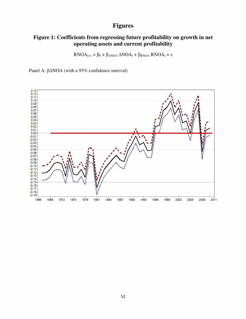
52
Figures
Figure 1: Coefficients from regressing future profitability on growth in net
operating assets and current profitability
RNOAt+1 = β0 + β∆NOA ∆NOAt + βRNOA RNOAt + ε
Panel A: β∆NOA (with a 95% confidence interval)
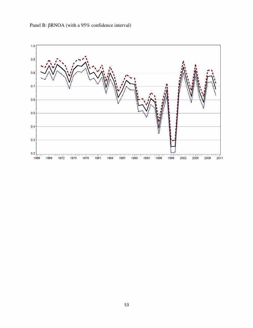
53
Panel B: βRNOA (with a 95% confidence interval)
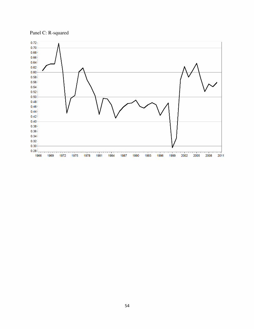
54
Panel C: R-squared
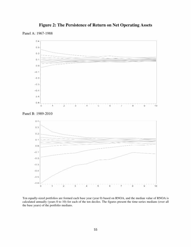
55
Figure 2: The Persistence of Return on Net Operating Assets
Panel A: 1967-1988
Panel B: 1989-2010
Ten equally-sized portfolios are formed each base year (year 0) based on RNOA, and the median value of RNOA is
calculated annually (years 0 to 10) for each of the ten deciles. The figures present the time-series medians (over all
the base years) of the portfolio medians.
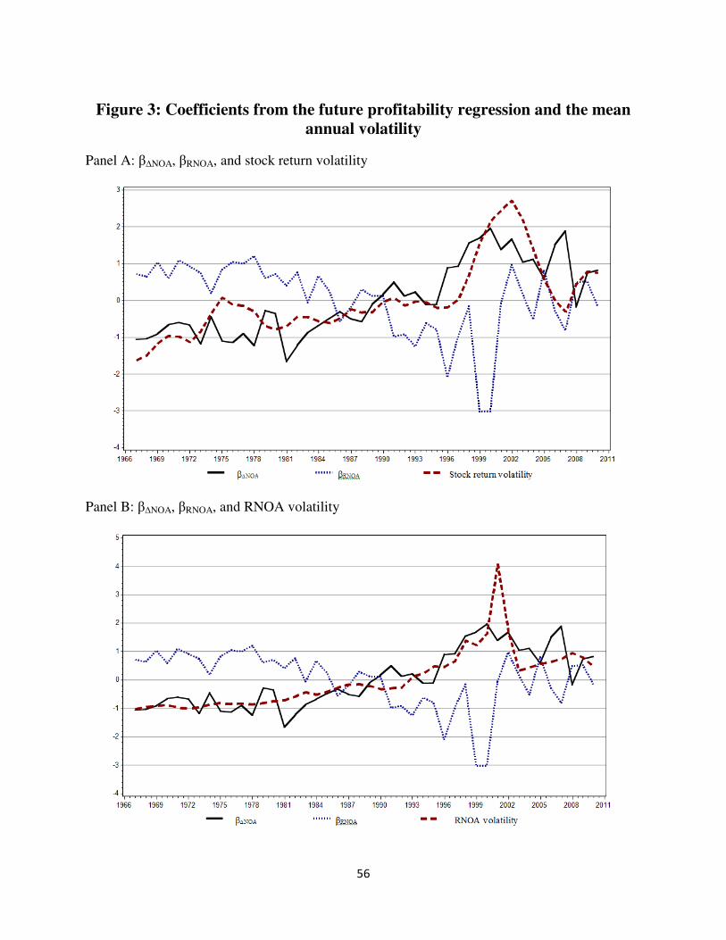
56
Figure 3: Coefficients from the future profitability regression and the mean
annual volatility
Panel A: β∆NOA, βRNOA, and stock return volatility
Panel B: β∆NOA, βRNOA, and RNOA volatility
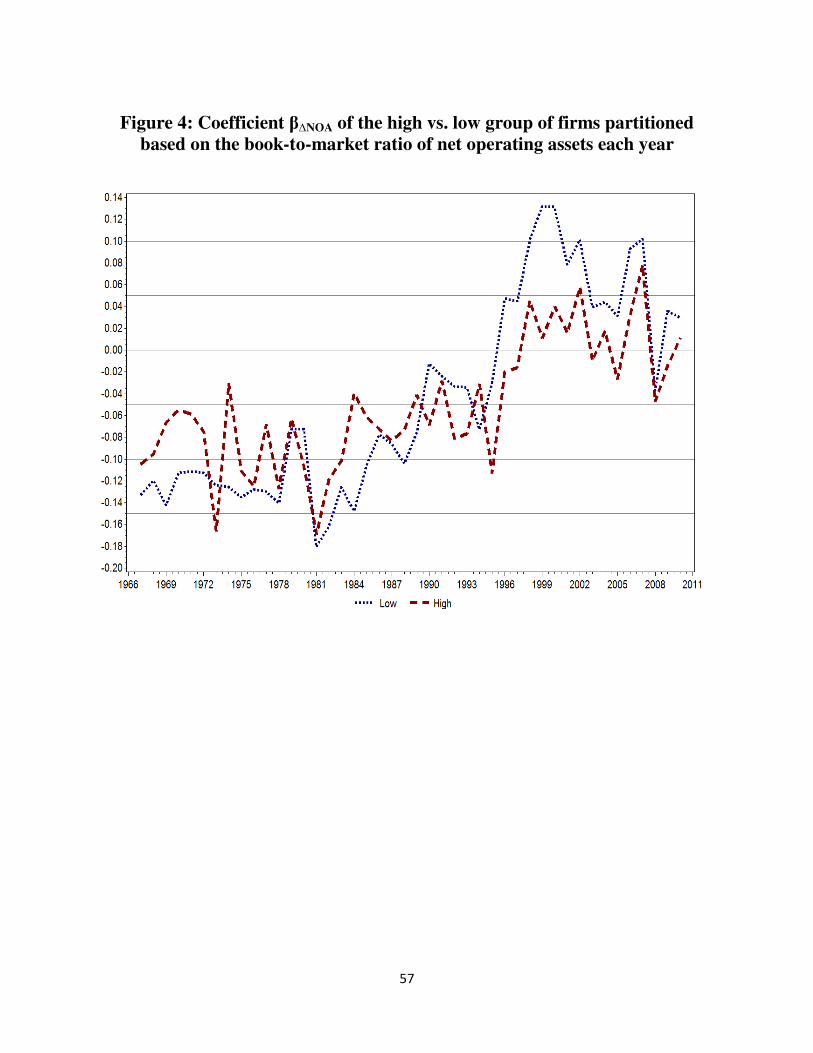
57
Figure 4: Coefficient β∆NOA of the high vs. low group of firms partitioned
based on the book-to-market ratio of net operating assets each year
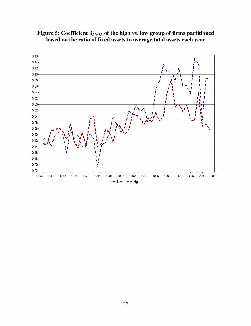
58
Figure 5: Coefficient β∆NOA of the high vs. low group of firms partitioned
based on the ratio of fixed assets to average total assets each year
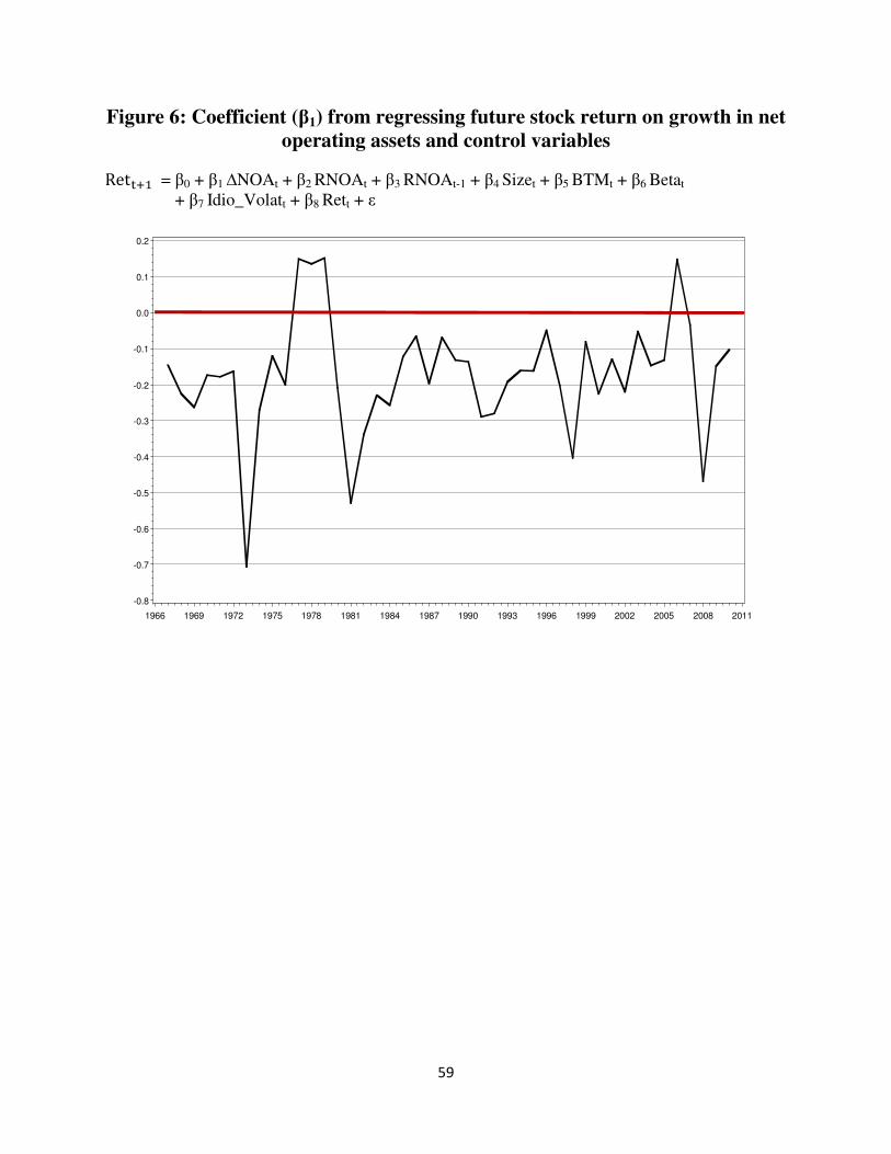
59
Figure 6: Coefficient (β1) from regressing future stock return on growth in net
operating assets and control variables
Ret��� = β0 + β1 ∆NOAt + β2 RNOAt + β3 RNOAt-1 + β4 Sizet + β5 BTMt + β6 Betat
+ β7 Idio_Volatt + β8 Rett + ε
-0.8
-0.7
-0.6
-0.5
-0.4
-0.3
-0.2
-0.1
0.0
0.1
0.2
1966 1969 1972 1975 1978 1981 1984 1987 1990 1993 1996 1999 2002 2005 2008 2011
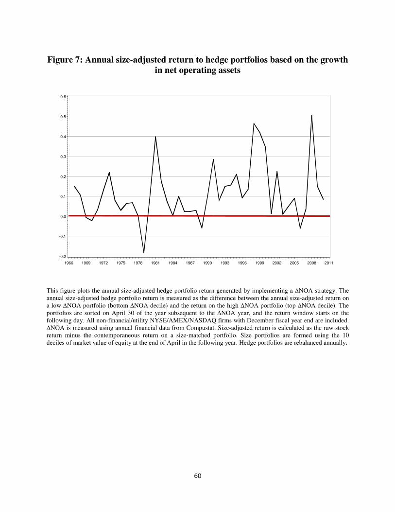
60
Figure 7: Annual size-adjusted return to hedge portfolios based on the growth
in net operating assets
This figure plots the annual size-adjusted hedge portfolio return generated by implementing a ∆NOA strategy. The
annual size-adjusted hedge portfolio return is measured as the difference between the annual size-adjusted return on
a low ∆NOA portfolio (bottom ∆NOA decile) and the return on the high ∆NOA portfolio (top ∆NOA decile). The
portfolios are sorted on April 30 of the year subsequent to the ∆NOA year, and the return window starts on the
following day. All non-financial/utility NYSE/AMEX/NASDAQ firms with December fiscal year end are included.
∆NOA is measured using annual financial data from Compustat. Size-adjusted return is calculated as the raw stock
return minus the contemporaneous return on a size-matched portfolio. Size portfolios are formed using the 10
deciles of market value of equity at the end of April in the following year. Hedge portfolios are rebalanced annually.
-0.2
-0.1
0.0
0.1
0.2
0.3
0.4
0.5
0.6
1966 1969 1972 1975 1978 1981 1984 1987 1990 1993 1996 1999 2002 2005 2008 2011
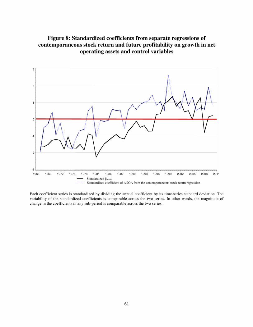
61
Figure 8: Standardized coefficients from separate regressions of
contemporaneous stock return and future profitability on growth in net
operating assets and control variables
Each coefficient series is standardized by dividing the annual coefficient by its time-series standard deviation. The
variability of the standardized coefficients is comparable across the two series. In other words, the magnitude of
change in the coefficients in any sub-period is comparable across the two series.
-3
-2
-1
0
1
2
3
1966 1969 1972 1975 1978 1981 1984 1987 1990 1993 1996 1999 2002 2005 2008 2011
Standardized β∆NOA
Standardized coefficient of ∆NOA from the contemporaneous stock return regression
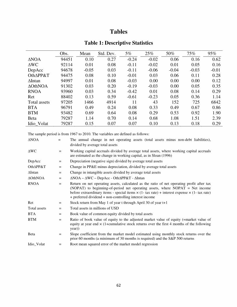
62
Tables
Table 1: Descriptive Statistics
Obs. Mean Std. Dev. 5% 25% 50% 75% 95%
∆NOA 94451 0.10 0.27 -0.24 -0.02 0.06 0.16 0.62
∆WC 92114 0.01 0.08 -0.11 -0.02 0.01 0.05 0.16
DepAcc 94678 -0.05 0.03 -0.11 -0.06 -0.04 -0.03 -0.01
Oth∆PP&T 94475 0.08 0.10 -0.01 0.03 0.06 0.11 0.28
∆Intan 94997 0.01 0.08 -0.03 0.00 0.00 0.00 0.12
∆OthNOA 91302 0.03 0.20 -0.19 -0.03 0.00 0.05 0.35
RNOA 93960 0.03 0.34 -0.42 0.01 0.08 0.14 0.29
Ret 88402 0.13 0.59 -0.61 -0.23 0.05 0.36 1.14
Total assets 97205 1466 4914 11 43 152 725 6842
BTA 96791 0.49 0.24 0.08 0.33 0.49 0.67 0.86
BTM 93482 0.69 0.64 0.08 0.29 0.53 0.92 1.90
Beta 79287 1.14 0.70 0.14 0.68 1.08 1.51 2.39
Idio_Volat 79287 0.15 0.07 0.07 0.10 0.13 0.18 0.29
The sample period is from 1967 to 2010. The variables are defined as follows:
∆NOA = The annual change in net operating assets (total assets minus non-debt liabilities),
divided by average total assets
∆WC = Working capital accruals divided by average total assets, where working capital accruals
are estimated as the change in working capital, as in Sloan (1996)
DepAcc = Depreciation (negative sign) divided by average total assets
Oth∆PP&T = Change in PP&E minus depreciation, divided by average total assets
∆Intan = Change in intangible assets divided by average total assets
∆OthNOA = ∆NOA – ∆WC – DepAcc - Oth∆PP&T - ∆Intan
RNOA = Return on net operating assets, calculated as the ratio of net operating profit after tax
(NOPAT) to beginning-of-period net operating assets, where NOPAT = Net income
before extraordinary items - special items × (1- tax rate) + interest expense × (1- tax rate)
+ preferred dividend + non-controlling interest income
Ret = Stock return from May 1 of year t through April 30 of year t+1
Total assets = Total assets in millions of USD
BTA = Book value of common equity divided by total assets
BTM = Ratio of book value of equity to the adjusted market value of equity (=market value of
equity at year end × (1+cumulative stock returns over the first 4 months of the following
year))
Beta = Slope coefficient from the market model estimated using monthly stock returns over the
prior 60 months (a minimum of 30 months is required) and the S&P 500 returns
Idio_Volat = Root mean squared error of the market model regression
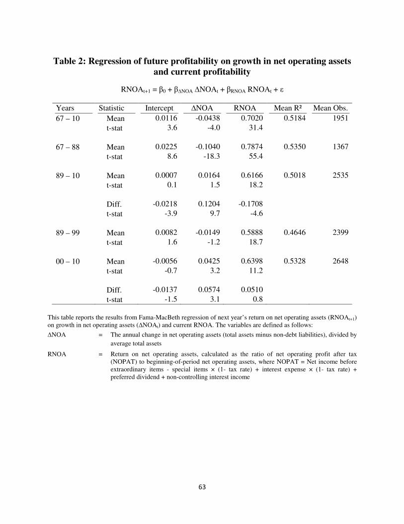
63
Table 2: Regression of future profitability on growth in net operating assets
and current profitability
RNOAt+1 = β0 + β∆NOA ∆NOAt + βRNOA RNOAt + ε
Years Statistic Intercept ∆NOA RNOA Mean R² Mean Obs.
67 – 10 Mean 0.0116 -0.0438 0.7020 0.5184 1951
t-stat 3.6 -4.0 31.4
67 – 88 Mean 0.0225 -0.1040 0.7874 0.5350 1367
t-stat 8.6 -18.3 55.4
89 – 10 Mean 0.0007 0.0164 0.6166 0.5018 2535
t-stat 0.1 1.5 18.2
Diff. -0.0218 0.1204 -0.1708
t-stat -3.9 9.7 -4.6
89 – 99 Mean 0.0082 -0.0149 0.5888 0.4646 2399
t-stat 1.6 -1.2 18.7
00 – 10 Mean -0.0056 0.0425 0.6398 0.5328 2648
t-stat -0.7 3.2 11.2
Diff. -0.0137 0.0574 0.0510
t-stat -1.5 3.1 0.8
This table reports the results from Fama-MacBeth regression of next year’s return on net operating assets (RNOAt+1)
on growth in net operating assets (∆NOAt) and current RNOA. The variables are defined as follows:
∆NOA = The annual change in net operating assets (total assets minus non-debt liabilities), divided by
average total assets
RNOA = Return on net operating assets, calculated as the ratio of net operating profit after tax
(NOPAT) to beginning-of-period net operating assets, where NOPAT = Net income before
extraordinary items - special items × (1- tax rate) + interest expense × (1- tax rate) +
preferred dividend + non-controlling interest income
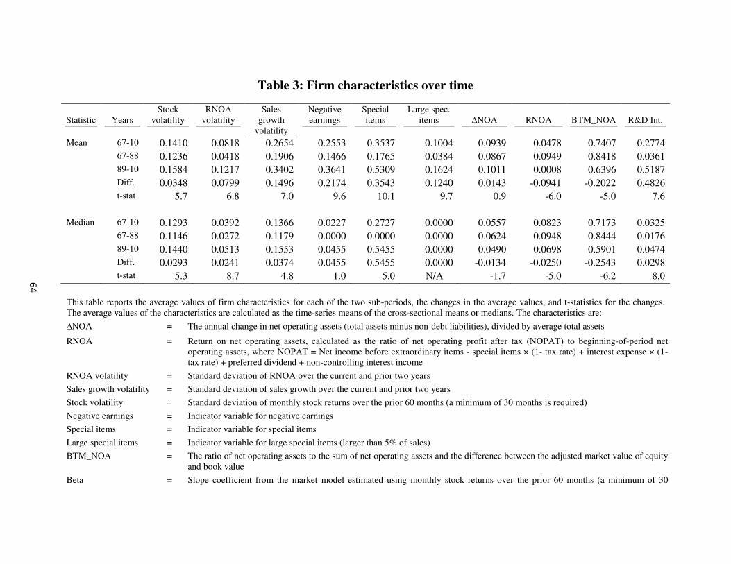
Table 3: Firm characteristics over time
Statistic
Years
Stock
volatility
RNOA
volatility
Sales
growth
volatility
Negative
earnings
Special
items
Large spec.
items
∆NOA
RNOA BTM_NOA
R&D Int.
Mean 67-10 0.1410 0.0818 0.2654 0.2553 0.3537 0.1004 0.0939 0.0478 0.7407 0.2774
67-88 0.1236 0.0418 0.1906 0.1466 0.1765 0.0384 0.0867 0.0949 0.8418 0.0361
89-10 0.1584 0.1217 0.3402 0.3641 0.5309 0.1624 0.1011 0.0008 0.6396 0.5187
Diff. 0.0348 0.0799 0.1496 0.2174 0.3543 0.1240 0.0143 -0.0941 -0.2022 0.4826
t-stat 5.7 6.8 7.0 9.6 10.1 9.7 0.9 -6.0 -5.0 7.6
Median 67-10 0.1293 0.0392 0.1366 0.0227 0.2727 0.0000 0.0557 0.0823 0.7173 0.0325
67-88 0.1146 0.0272 0.1179 0.0000 0.0000 0.0000 0.0624 0.0948 0.8444 0.0176
89-10 0.1440 0.0513 0.1553 0.0455 0.5455 0.0000 0.0490 0.0698 0.5901 0.0474
Diff. 0.0293 0.0241 0.0374 0.0455 0.5455 0.0000 -0.0134 -0.0250 -0.2543 0.0298
t-stat 5.3 8.7 4.8 1.0 5.0 N/A -1.7 -5.0 -6.2 8.0
This table reports the average values of firm characteristics for each of the two sub-periods, the changes in the average values, and t-statistics for the changes.
The average values of the characteristics are calculated as the time-series means of the cross-sectional means or medians. The characteristics are:
∆NOA = The annual change in net operating assets (total assets minus non-debt liabilities), divided by average total assets
RNOA = Return on net operating assets, calculated as the ratio of net operating profit after tax (NOPAT) to beginning-of-period net
operating assets, where NOPAT = Net income before extraordinary items - special items × (1- tax rate) + interest expense × (1-
tax rate) + preferred dividend + non-controlling interest income
RNOA volatility = Standard deviation of RNOA over the current and prior two years
Sales growth volatility = Standard deviation of sales growth over the current and prior two years
Stock volatility = Standard deviation of monthly stock returns over the prior 60 months (a minimum of 30 months is required)
Negative earnings = Indicator variable for negative earnings
Special items = Indicator variable for special items
Large special items = Indicator variable for large special items (larger than 5% of sales)
BTM_NOA = The ratio of net operating assets to the sum of net operating assets and the difference between the adjusted market value of equity
and book value
Beta = Slope coefficient from the market model estimated using monthly stock returns over the prior 60 months (a minimum of 30
64

months is required) and the S&P 500 returns
R&D intensity = R&D expense divided by sales
65
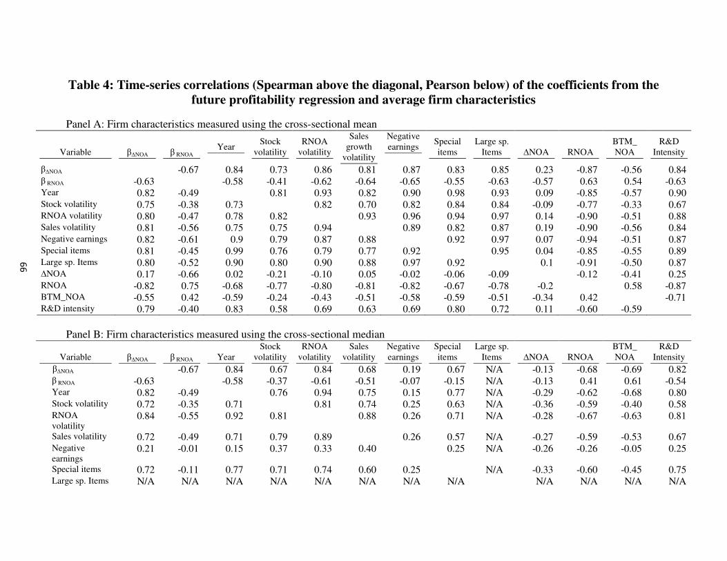
Table 4: Time-series correlations (Spearman above the diagonal, Pearson below) of the coefficients from the
future profitability regression and average firm characteristics
Panel A: Firm characteristics measured using the cross-sectional mean
Variable
β∆NOA
β RNOA
Year Stock
volatility
RNOA
volatility
Sales
growth
volatility
Negative
earnings Special
items
Large sp.
Items
∆NOA
RNOA
BTM_
NOA
R&D
Intensity
β∆NOA -0.67 0.84 0.73 0.86 0.81 0.87 0.83 0.85 0.23 -0.87 -0.56 0.84 β RNOA -0.63 -0.58 -0.41 -0.62 -0.64 -0.65 -0.55 -0.63 -0.57 0.63 0.54 -0.63 Year 0.82 -0.49 0.81 0.93 0.82 0.90 0.98 0.93 0.09 -0.85 -0.57 0.90 Stock volatility 0.75 -0.38 0.73 0.82 0.70 0.82 0.84 0.84 -0.09 -0.77 -0.33 0.67 RNOA volatility 0.80 -0.47 0.78 0.82 0.93 0.96 0.94 0.97 0.14 -0.90 -0.51 0.88 Sales volatility 0.81 -0.56 0.75 0.75 0.94 0.89 0.82 0.87 0.19 -0.90 -0.56 0.84 Negative earnings 0.82 -0.61 0.9 0.79 0.87 0.88 0.92 0.97 0.07 -0.94 -0.51 0.87 Special items 0.81 -0.45 0.99 0.76 0.79 0.77 0.92 0.95 0.04 -0.85 -0.55 0.89 Large sp. Items 0.80 -0.52 0.90 0.80 0.90 0.88 0.97 0.92 0.1 -0.91 -0.50 0.87 ∆NOA 0.17 -0.66 0.02 -0.21 -0.10 0.05 -0.02 -0.06 -0.09 -0.12 -0.41 0.25 RNOA -0.82 0.75 -0.68 -0.77 -0.80 -0.81 -0.82 -0.67 -0.78 -0.2 0.58 -0.87 BTM_NOA -0.55 0.42 -0.59 -0.24 -0.43 -0.51 -0.58 -0.59 -0.51 -0.34 0.42 -0.71 R&D intensity 0.79 -0.40 0.83 0.58 0.69 0.63 0.69 0.80 0.72 0.11 -0.60 -0.59
Panel B: Firm characteristics measured using the cross-sectional median
Variable
β∆NOA
β RNOA
Year
Stock
volatility
RNOA
volatility
Sales
volatility
Negative
earnings
Special
items
Large sp.
Items
∆NOA
RNOA
BTM_
NOA
R&D
Intensity
β∆NOA -0.67 0.84 0.67 0.84 0.68 0.19 0.67 N/A -0.13 -0.68 -0.69 0.82 β RNOA -0.63 -0.58 -0.37 -0.61 -0.51 -0.07 -0.15 N/A -0.13 0.41 0.61 -0.54 Year 0.82 -0.49 0.76 0.94 0.75 0.15 0.77 N/A -0.29 -0.62 -0.68 0.80 Stock volatility 0.72 -0.35 0.71 0.81 0.74 0.25 0.63 N/A -0.36 -0.59 -0.40 0.58 RNOA
volatility 0.84 -0.55 0.92 0.81 0.88 0.26 0.71 N/A -0.28 -0.67 -0.63 0.81
Sales volatility 0.72 -0.49 0.71 0.79 0.89 0.26 0.57 N/A -0.27 -0.59 -0.53 0.67 Negative
earnings 0.21 -0.01 0.15 0.37 0.33 0.40 0.25 N/A -0.26 -0.26 -0.05 0.25
Special items 0.72 -0.11 0.77 0.71 0.74 0.60 0.25 N/A -0.33 -0.60 -0.45 0.75 Large sp. Items N/A N/A N/A N/A N/A N/A N/A N/A N/A N/A N/A N/A
66
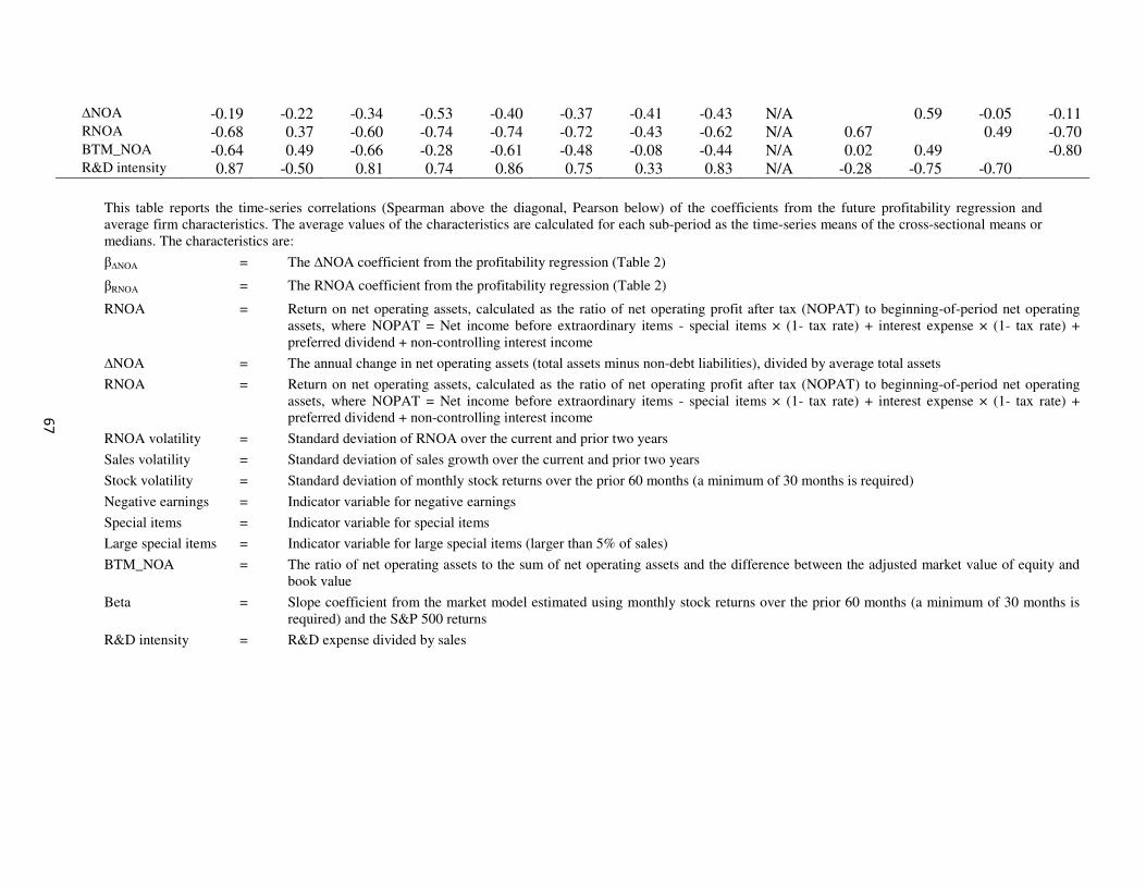
∆NOA -0.19 -0.22 -0.34 -0.53 -0.40 -0.37 -0.41 -0.43 N/A 0.59 -0.05 -0.11 RNOA -0.68 0.37 -0.60 -0.74 -0.74 -0.72 -0.43 -0.62 N/A 0.67 0.49 -0.70 BTM_NOA -0.64 0.49 -0.66 -0.28 -0.61 -0.48 -0.08 -0.44 N/A 0.02 0.49 -0.80 R&D intensity 0.87 -0.50 0.81 0.74 0.86 0.75 0.33 0.83 N/A -0.28 -0.75 -0.70
This table reports the time-series correlations (Spearman above the diagonal, Pearson below) of the coefficients from the future profitability regression and
average firm characteristics. The average values of the characteristics are calculated for each sub-period as the time-series means of the cross-sectional means or
medians. The characteristics are:
β∆NOA = The ∆NOA coefficient from the profitability regression (Table 2)
βRNOA = The RNOA coefficient from the profitability regression (Table 2)
RNOA = Return on net operating assets, calculated as the ratio of net operating profit after tax (NOPAT) to beginning-of-period net operating
assets, where NOPAT = Net income before extraordinary items - special items × (1- tax rate) + interest expense × (1- tax rate) +
preferred dividend + non-controlling interest income
∆NOA = The annual change in net operating assets (total assets minus non-debt liabilities), divided by average total assets
RNOA = Return on net operating assets, calculated as the ratio of net operating profit after tax (NOPAT) to beginning-of-period net operating
assets, where NOPAT = Net income before extraordinary items - special items × (1- tax rate) + interest expense × (1- tax rate) +
preferred dividend + non-controlling interest income
RNOA volatility = Standard deviation of RNOA over the current and prior two years
Sales volatility = Standard deviation of sales growth over the current and prior two years
Stock volatility = Standard deviation of monthly stock returns over the prior 60 months (a minimum of 30 months is required)
Negative earnings = Indicator variable for negative earnings
Special items = Indicator variable for special items
Large special items = Indicator variable for large special items (larger than 5% of sales)
BTM_NOA = The ratio of net operating assets to the sum of net operating assets and the difference between the adjusted market value of equity and
book value
Beta = Slope coefficient from the market model estimated using monthly stock returns over the prior 60 months (a minimum of 30 months is
required) and the S&P 500 returns
R&D intensity = R&D expense divided by sales
67
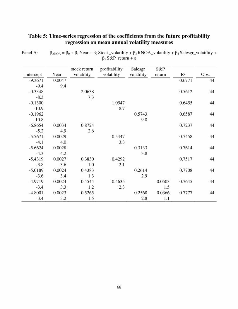
68
Table 5: Time-series regression of the coefficients from the future profitability
regression on mean annual volatility measures
Panel A: β∆NOA = β0 + β1 Year + β2 Stock_volatility + β3 RNOA_volatility + β4 Salesgr_volatility +
β5 S&P_return + ε
Intercept
Year
stock return
volatility
profitability
volatility
Salesgr
volatility
S&P
return
R²
Obs.
-9.3671 0.0047 0.6771 44
-9.4 9.4
-0.3348 2.0638 0.5612 44
-8.3 7.3
-0.1300 1.0547 0.6455 44
-10.9 8.7
-0.1962 0.5743 0.6587 44
-10.8 9.0
-6.8654 0.0034 0.8724 0.7237 44
-5.2 4.9 2.6
-5.7671 0.0029 0.5447 0.7458 44
-4.1 4.0 3.3
-5.6624 0.0028 0.3133 0.7614 44
-4.3 4.2 3.8
-5.4319 0.0027 0.3830 0.4292 0.7517 44
-3.8 3.6 1.0 2.1
-5.0189 0.0024 0.4383 0.2614 0.7708 44
-3.6 3.4 1.3 2.9
-4.9719 0.0024 0.4544 0.4635 0.0503 0.7645 44
-3.4 3.3 1.2 2.3 1.5
-4.8001 0.0023 0.5265 0.2568 0.0366 0.7777 44
-3.4 3.2 1.5 2.8 1.1
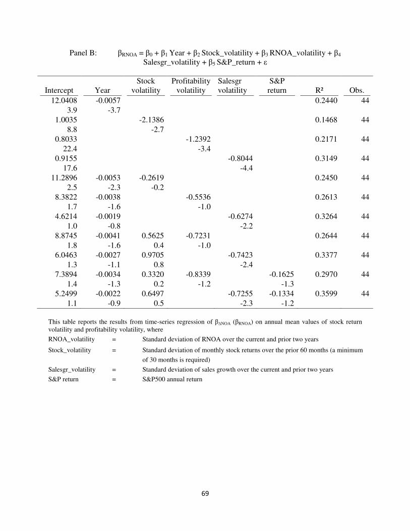
69
Panel B: βRNOA = β0 + β1 Year + β2 Stock_volatility + β3 RNOA_volatility + β4
Salesgr_volatility + β5 S&P_return + ε
Intercept
Year
Stock
volatility
Profitability
volatility
Salesgr
volatility
S&P
return
R²
Obs.
12.0408 -0.0057 0.2440 44
3.9 -3.7
1.0035 -2.1386 0.1468 44
8.8 -2.7
0.8033 -1.2392 0.2171 44
22.4 -3.4
0.9155 -0.8044 0.3149 44
17.6 -4.4
11.2896 -0.0053 -0.2619 0.2450 44
2.5 -2.3 -0.2
8.3822 -0.0038 -0.5536 0.2613 44
1.7 -1.6 -1.0
4.6214 -0.0019 -0.6274 0.3264 44
1.0 -0.8 -2.2
8.8745 -0.0041 0.5625 -0.7231 0.2644 44
1.8 -1.6 0.4 -1.0
6.0463 -0.0027 0.9705 -0.7423 0.3377 44
1.3 -1.1 0.8 -2.4
7.3894 -0.0034 0.3320 -0.8339 -0.1625 0.2970 44
1.4 -1.3 0.2 -1.2 -1.3
5.2499 -0.0022 0.6497 -0.7255 -0.1334 0.3599 44
1.1 -0.9 0.5 -2.3 -1.2
This table reports the results from time-series regression of β∆NOA (βRNOA) on annual mean values of stock return
volatility and profitability volatility, where
RNOA_volatility = Standard deviation of RNOA over the current and prior two years
Stock_volatility = Standard deviation of monthly stock returns over the prior 60 months (a minimum
of 30 months is required)
Salesgr_volatility = Standard deviation of sales growth over the current and prior two years
S&P return = S&P500 annual return
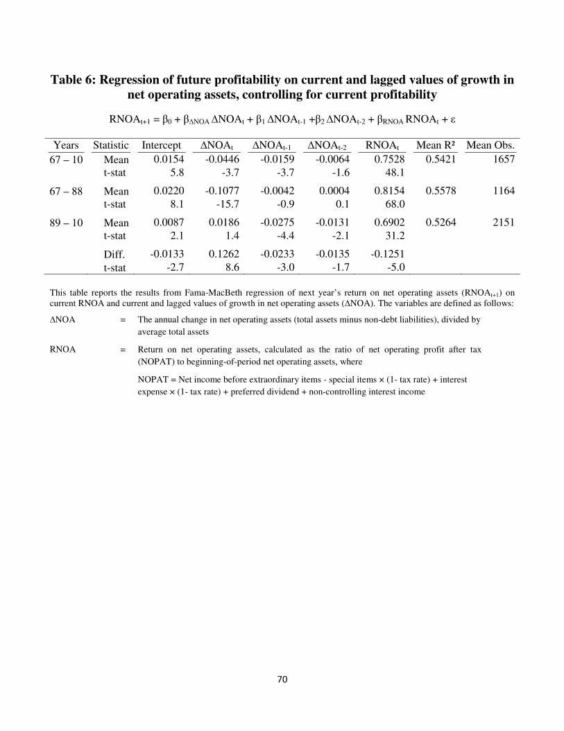
70
Table 6: Regression of future profitability on current and lagged values of growth in
net operating assets, controlling for current profitability
RNOAt+1 = β0 + β∆NOA ∆NOAt + β1 ∆NOAt-1 +β2 ∆NOAt-2 + βRNOA RNOAt + ε
Years Statistic Intercept ∆NOAt ∆NOAt-1 ∆NOAt-2 RNOAt Mean R² Mean Obs.
67 – 10 Mean 0.0154 -0.0446 -0.0159 -0.0064 0.7528 0.5421 1657
t-stat 5.8 -3.7 -3.7 -1.6 48.1
67 – 88 Mean 0.0220 -0.1077 -0.0042 0.0004 0.8154 0.5578 1164
t-stat 8.1 -15.7 -0.9 0.1 68.0
89 – 10 Mean 0.0087 0.0186 -0.0275 -0.0131 0.6902 0.5264 2151
t-stat 2.1 1.4 -4.4 -2.1 31.2
Diff. -0.0133 0.1262 -0.0233 -0.0135 -0.1251
t-stat -2.7 8.6 -3.0 -1.7 -5.0
This table reports the results from Fama-MacBeth regression of next year’s return on net operating assets (RNOAt+1) on
current RNOA and current and lagged values of growth in net operating assets (∆NOA). The variables are defined as follows:
∆NOA = The annual change in net operating assets (total assets minus non-debt liabilities), divided by
average total assets
RNOA = Return on net operating assets, calculated as the ratio of net operating profit after tax
(NOPAT) to beginning-of-period net operating assets, where
NOPAT = Net income before extraordinary items - special items × (1- tax rate) + interest
expense × (1- tax rate) + preferred dividend + non-controlling interest income
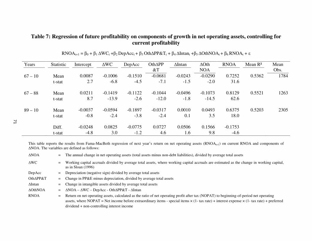
Table 7: Regression of future profitability on components of growth in net operating assets, controlling for
current profitability
RNOAt+1 = β0 + β1 ∆WCt +β2 DepAcct + β3 Oth∆PP&Tt + β4 ∆Intant +β5 ∆OthNOAt + β6 RNOAt + ε
Years Statistic Intercept ∆WC DepAcc Oth∆PP
&T
∆Intan ∆Oth
NOA
RNOA Mean R² Mean
Obs.
67 – 10 Mean 0.0087 -0.1006 -0.1510 -0.0681 -0.0243 -0.0290 0.7252 0.5362 1784
t-stat 2.7 -6.8 -4.5 -7.1 -1.5 -2.0 31.6
67 – 88 Mean 0.0211 -0.1419 -0.1122 -0.1044 -0.0496 -0.1073 0.8129 0.5521 1263
t-stat 8.7 -13.9 -2.6 -12.0 -1.8 -14.5 62.6
89 – 10 Mean -0.0037 -0.0594 -0.1897 -0.0317 0.0010 0.0493 0.6375 0.5203 2305
t-stat -0.8 -2.4 -3.8 -2.4 0.1 3.5 18.0
Diff. -0.0248 0.0825 -0.0775 0.0727 0.0506 0.1566 -0.1753
t-stat -4.8 3.0 -1.2 4.6 1.6 9.8 -4.6
This table reports the results from Fama-MacBeth regression of next year’s return on net operating assets (RNOAt+1) on current RNOA and components of
∆NOA. The variables are defined as follows:
∆NOA = The annual change in net operating assets (total assets minus non-debt liabilities), divided by average total assets
∆WC = Working capital accruals divided by average total assets, where working capital accruals are estimated as the change in working capital,
as in Sloan (1996)
DepAcc = Depreciation (negative sign) divided by average total assets
Oth∆PP&T = Change in PP&E minus depreciation, divided by average total assets
∆Intan = Change in intangible assets divided by average total assets
∆OthNOA = ∆NOA – ∆WC – DepAcc - Oth∆PP&T - ∆Intan
RNOA = Return on net operating assets, calculated as the ratio of net operating profit after tax (NOPAT) to beginning-of-period net operating
assets, where NOPAT = Net income before extraordinary items - special items × (1- tax rate) + interest expense × (1- tax rate) + preferred
dividend + non-controlling interest income
71
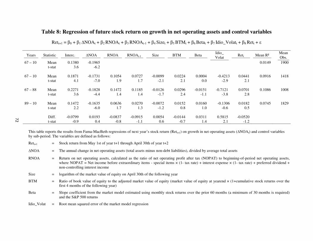
Table 8: Regression of future stock return on growth in net operating assets and control variables
Rett+1 = β0 + β1 ∆NOAt + β2 RNOAt + β3 RNOAt-1 + β4 Sizet + β5 BTMt + β6 Betat + β7 Idio_Volatt + β8 Rett + ε
Years Statistic Interc. ∆NOA RNOA RNOAt-1 Size BTM Beta Idio_
Volat Rett Mean R²
Mean
Obs.
67 – 10 Mean 0.1380 -0.1965 0.0149 1900
t-stat 3.6 -6.2
67 – 10 Mean 0.1871 -0.1731 0.1054 0.0727 -0.0099 0.0224 0.0004 -0.4213 0.0441 0.0916 1418
t-stat 4.1 -7.0 1.9 1.7 -2.1 2.1 0.0 -2.9 2.1
67 – 88 Mean 0.2271 -0.1828 0.1472 0.1185 -0.0126 0.0296 -0.0151 -0.7121 0.0701 0.1086 1008
t-stat 3.6 -4.4 1.4 1.4 -1.7 2.4 -1.1 -3.8 2.8
89 – 10 Mean 0.1472 -0.1635 0.0636 0.0270 -0.0072 0.0152 0.0160 -0.1306 0.0182 0.0745 1829
t-stat 2.2 -6.0 1.7 1.3 -1.2 0.8 1.0 -0.6 0.5
Diff. -0.0799 0.0193 -0.0837 -0.0915 0.0054 -0.0144 0.0311 0.5815 -0.0520
t-stat -0.9 0.4 -0.8 -1.1 0.6 -0.7 1.4 2.1 -1.2
This table reports the results from Fama-MacBeth regressions of next year’s stock return (Rett+1) on growth in net operating assets (∆NOAt) and control variables
by sub-period. The variables are defined as follows:
Rett+1 = Stock return from May 1st of year t+1 through April 30th of year t+2
∆NOA = The annual change in net operating assets (total assets minus non-debt liabilities), divided by average total assets
RNOA = Return on net operating assets, calculated as the ratio of net operating profit after tax (NOPAT) to beginning-of-period net operating assets,
where NOPAT = Net income before extraordinary items - special items × (1- tax rate) + interest expense × (1- tax rate) + preferred dividend +
non-controlling interest income
Size = logarithm of the market value of equity on April 30th of the following year
BTM = Ratio of book value of equity to the adjusted market value of equity (market value of equity at yearend × (1+cumulative stock returns over the
first 4 months of the following year)
Beta = Slope coefficient from the market model estimated using monthly stock returns over the prior 60 months (a minimum of 30 months is required)
and the S&P 500 returns
Idio_Volat = Root mean squared error of the market model regression
72
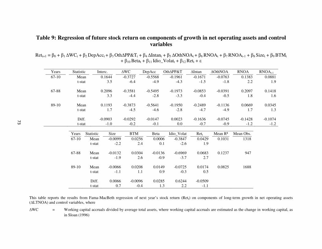
Table 9: Regression of future stock return on components of growth in net operating assets and control
variables
Rett+1 = β0 + β1 ∆WCt + β2 DepAcct + β3 Oth∆PP&Tt + β4 ∆Intant + β5 ∆OthNOAt + β6 RNOAt + β7 RNOAt-1 + β8 Sizet + β9 BTMt
+ β10 Betat + β11 Idio_Volatt + β12 Rett + ε
Years Statistic Interc. ∆WC DepAcc Oth∆PP&T ∆Intan ∆OthNOA RNOA RNOAt-1
67-10 Mean 0.1644 -0.3727 -0.5568 -0.1961 -0.1671 -0.0763 0.1383 0.0881
t-stat 3.5 -6.4 -4.9 -4.3 -1.5 -1.8 2.2 1.9
67-88 Mean 0.2096 -0.3581 -0.5495 -0.1973 -0.0853 -0.0391 0.2097 0.1418
t-stat 3.3 -4.4 -2.8 -3.3 -0.4 -0.5 1.8 1.6
89-10 Mean 0.1193 -0.3873 -0.5641 -0.1950 -0.2489 -0.1136 0.0669 0.0345
t-stat 1.7 -4.5 -4.6 -2.8 -4.7 -4.9 1.7 1.3
Diff. -0.0903 -0.0292 -0.0147 0.0023 -0.1636 -0.0745 -0.1428 -0.1074
t-stat -1.0 -0.2 -0.1 0.0 -0.7 -0.9 -1.2 -1.2
Years Statistic Size BTM Beta Idio_Volat Rett Mean R² Mean Obs.
67-10 Mean -0.0099 0.0256 0.0006 -0.3847 0.0429 0.1031 1318
t-stat -2.2 2.4 0.1 -2.6 1.9
67-88 Mean -0.0132 0.0304 -0.0136 -0.6969 0.0683 0.1237 947
t-stat -1.9 2.6 -0.9 -3.7 2.7
89-10 Mean -0.0066 0.0208 0.0149 -0.0725 0.0174 0.0825 1688
t-stat -1.1 1.1 0.9 -0.3 0.5
Diff. 0.0066 -0.0096 0.0285 0.6244 -0.0509
t-stat 0.7 -0.4 1.3 2.2 -1.1
This table reports the results from Fama-MacBeth regression of next year’s stock return (Rett) on components of long-term growth in net operating assets
(∆LTNOA) and control variables, where
∆WC = Working capital accruals divided by average total assets, where working capital accruals are estimated as the change in working capital, as
in Sloan (1996)
73

DepAcc = Depreciation (negative sign) divided by average total assets
Oth∆PP&T = Change in PP&E minus depreciation, divided by average total assets
∆Intan = Change in intangible assets divided by average total assets
∆OthNOA = ∆NOA – ∆WC – DepAcc - Oth∆PP&T - ∆Intan
and the other variables are as defined in Table 8.
74
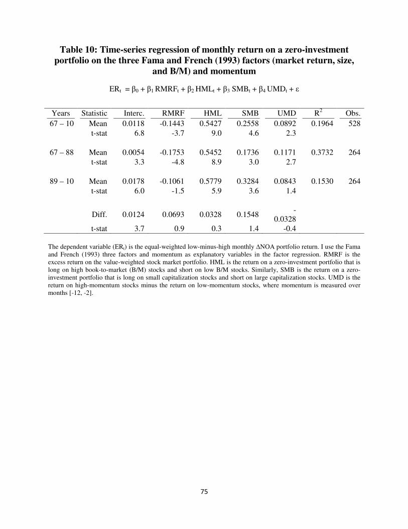
75
Table 10: Time-series regression of monthly return on a zero-investment
portfolio on the three Fama and French (1993) factors (market return, size,
and B/M) and momentum
ERt = β0 + β1 RMRFt + β2 HMLt + β3 SMBt + β4 UMDt + ε
Years Statistic Interc. RMRF HML SMB UMD R2
Obs.
67 – 10 Mean 0.0118 -0.1443 0.5427 0.2558 0.0892 0.1964 528
t-stat 6.8 -3.7 9.0 4.6 2.3
67 – 88 Mean 0.0054 -0.1753 0.5452 0.1736 0.1171 0.3732 264
t-stat 3.3 -4.8 8.9 3.0 2.7
89 – 10 Mean 0.0178 -0.1061 0.5779 0.3284 0.0843 0.1530 264
t-stat 6.0 -1.5 5.9 3.6 1.4
Diff. 0.0124 0.0693 0.0328 0.1548 -
0.0328
t-stat 3.7 0.9 0.3 1.4 -0.4
The dependent variable (ERt) is the equal-weighted low-minus-high monthly ∆NOA portfolio return. I use the Fama
and French (1993) three factors and momentum as explanatory variables in the factor regression. RMRF is the
excess return on the value-weighted stock market portfolio. HML is the return on a zero-investment portfolio that is
long on high book-to-market (B/M) stocks and short on low B/M stocks. Similarly, SMB is the return on a zero-
investment portfolio that is long on small capitalization stocks and short on large capitalization stocks. UMD is the
return on high-momentum stocks minus the return on low-momentum stocks, where momentum is measured over
months [-12, -2].
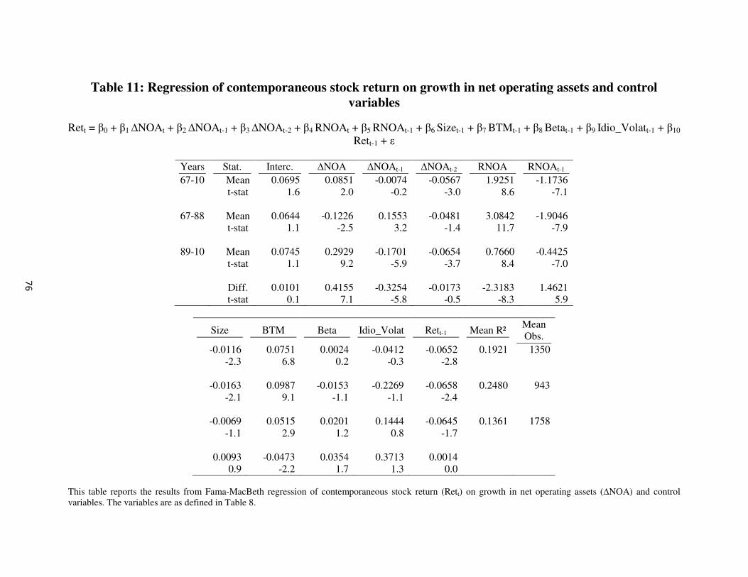
Table 11: Regression of contemporaneous stock return on growth in net operating assets and control
variables
Rett = β0 + β1 ∆NOAt + β2 ∆NOAt-1 + β3 ∆NOAt-2 + β4 RNOAt + β5 RNOAt-1 + β6 Sizet-1 + β7 BTMt-1 + β8 Betat-1 + β9 Idio_Volatt-1 + β10
Rett-1 + ε
Years Stat. Interc. ∆NOA ∆NOAt-1 ∆NOAt-2 RNOA RNOAt-1
67-10 Mean 0.0695 0.0851 -0.0074 -0.0567 1.9251 -1.1736
t-stat 1.6 2.0 -0.2 -3.0 8.6 -7.1
67-88 Mean 0.0644 -0.1226 0.1553 -0.0481 3.0842 -1.9046
t-stat 1.1 -2.5 3.2 -1.4 11.7 -7.9
89-10 Mean 0.0745 0.2929 -0.1701 -0.0654 0.7660 -0.4425
t-stat 1.1 9.2 -5.9 -3.7 8.4 -7.0
Diff. 0.0101 0.4155 -0.3254 -0.0173 -2.3183 1.4621
t-stat 0.1 7.1 -5.8 -0.5 -8.3 5.9
Size BTM Beta Idio_Volat Rett-1 Mean R² Mean
Obs.
-0.0116 0.0751 0.0024 -0.0412 -0.0652 0.1921 1350
-2.3 6.8 0.2 -0.3 -2.8
-0.0163 0.0987 -0.0153 -0.2269 -0.0658 0.2480 943
-2.1 9.1 -1.1 -1.1 -2.4
-0.0069 0.0515 0.0201 0.1444 -0.0645 0.1361 1758
-1.1 2.9 1.2 0.8 -1.7
0.0093 -0.0473 0.0354 0.3713 0.0014
0.9 -2.2 1.7 1.3 0.0
This table reports the results from Fama-MacBeth regression of contemporaneous stock return (Rett) on growth in net operating assets (∆NOA) and control
variables. The variables are as defined in Table 8.
76
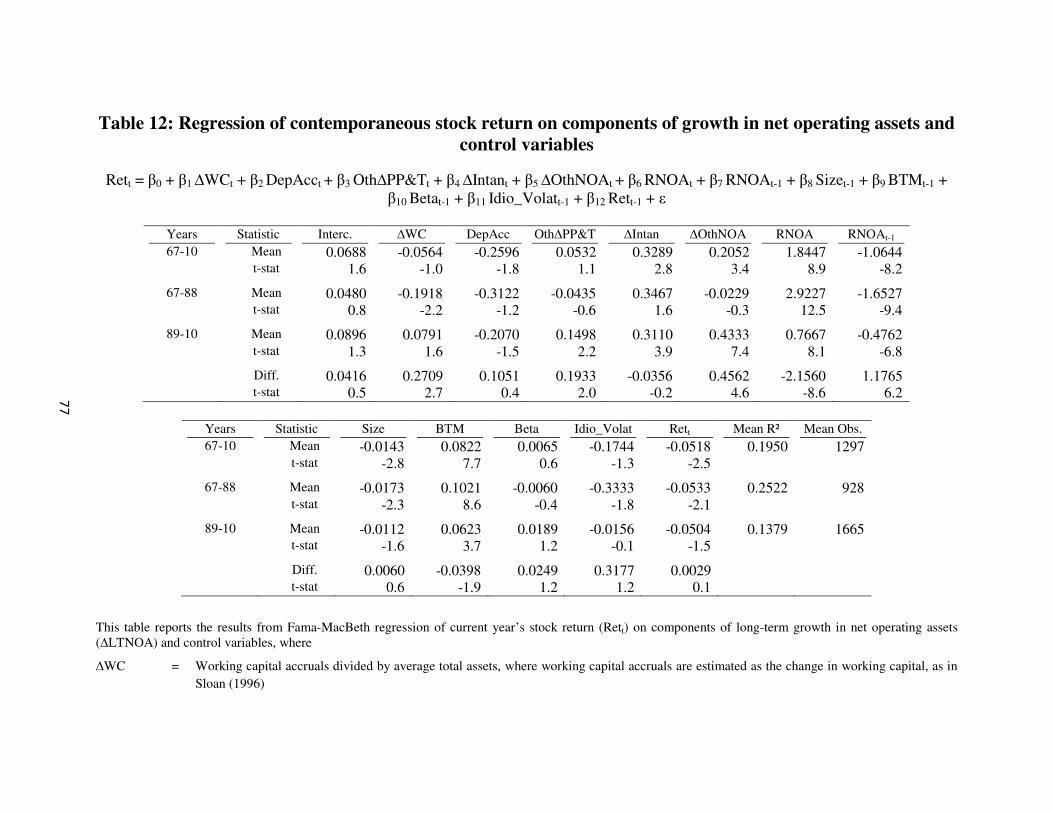
Table 12: Regression of contemporaneous stock return on components of growth in net operating assets and
control variables
Rett = β0 + β1 ∆WCt + β2 DepAcct + β3 Oth∆PP&Tt + β4 ∆Intant + β5 ∆OthNOAt + β6 RNOAt + β7 RNOAt-1 + β8 Sizet-1 + β9 BTMt-1 +
β10 Betat-1 + β11 Idio_Volatt-1 + β12 Rett-1 + ε
Years Statistic Interc. ∆WC DepAcc Oth∆PP&T ∆Intan ∆OthNOA RNOA RNOAt-1
67-10 Mean 0.0688 -0.0564 -0.2596 0.0532 0.3289 0.2052 1.8447 -1.0644
t-stat 1.6 -1.0 -1.8 1.1 2.8 3.4 8.9 -8.2
67-88 Mean 0.0480 -0.1918 -0.3122 -0.0435 0.3467 -0.0229 2.9227 -1.6527
t-stat 0.8 -2.2 -1.2 -0.6 1.6 -0.3 12.5 -9.4
89-10 Mean 0.0896 0.0791 -0.2070 0.1498 0.3110 0.4333 0.7667 -0.4762
t-stat 1.3 1.6 -1.5 2.2 3.9 7.4 8.1 -6.8
Diff. 0.0416 0.2709 0.1051 0.1933 -0.0356 0.4562 -2.1560 1.1765 t-stat 0.5 2.7 0.4 2.0 -0.2 4.6 -8.6 6.2
Years Statistic Size BTM Beta Idio_Volat Rett Mean R² Mean Obs.
67-10 Mean -0.0143 0.0822 0.0065 -0.1744 -0.0518 0.1950 1297
t-stat -2.8 7.7 0.6 -1.3 -2.5
67-88 Mean -0.0173 0.1021 -0.0060 -0.3333 -0.0533 0.2522 928
t-stat -2.3 8.6 -0.4 -1.8 -2.1
89-10 Mean -0.0112 0.0623 0.0189 -0.0156 -0.0504 0.1379 1665
t-stat -1.6 3.7 1.2 -0.1 -1.5
Diff. 0.0060 -0.0398 0.0249 0.3177 0.0029 t-stat 0.6 -1.9 1.2 1.2 0.1
This table reports the results from Fama-MacBeth regression of current year’s stock return (Rett) on components of long-term growth in net operating assets
(∆LTNOA) and control variables, where
∆WC = Working capital accruals divided by average total assets, where working capital accruals are estimated as the change in working capital, as in
Sloan (1996)
77

DepAcc = Depreciation (negative sign) divided by average total assets
Oth∆PP&T = Change in PP&E minus depreciation, divided by average total assets
∆Intan = Change in intangible assets divided by average total assets
∆OthNOA = ∆NOA – ∆WC – DepAcc - Oth∆PP&T - ∆Intan
and the other variables are as defined in Table 8.
78
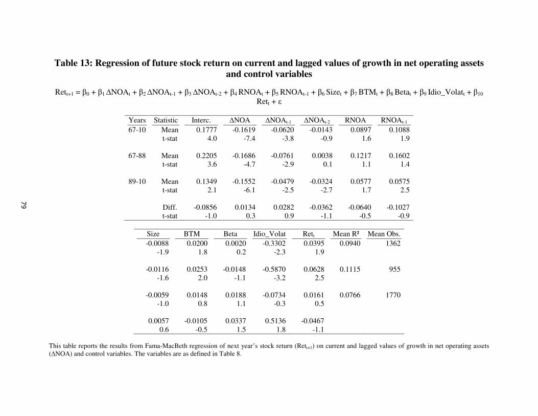
Table 13: Regression of future stock return on current and lagged values of growth in net operating assets
and control variables
Rett+1 = β0 + β1 ∆NOAt + β2 ∆NOAt-1 + β3 ∆NOAt-2 + β4 RNOAt + β5 RNOAt-1 + β6 Sizet + β7 BTMt + β8 Betat + β9 Idio_Volatt + β10
Rett + ε
Years Statistic Interc. ∆NOA ∆NOAt-1 ∆NOAt-2 RNOA RNOAt-1
67-10 Mean 0.1777 -0.1619 -0.0620 -0.0143 0.0897 0.1088
t-stat 4.0 -7.4 -3.8 -0.9 1.6 1.9
67-88 Mean 0.2205 -0.1686 -0.0761 0.0038 0.1217 0.1602
t-stat 3.6 -4.7 -2.9 0.1 1.1 1.4
89-10 Mean 0.1349 -0.1552 -0.0479 -0.0324 0.0577 0.0575
t-stat 2.1 -6.1 -2.5 -2.7 1.7 2.5
Diff. -0.0856 0.0134 0.0282 -0.0362 -0.0640 -0.1027
t-stat -1.0 0.3 0.9 -1.1 -0.5 -0.9
Size BTM Beta Idio_Volat Rett Mean R² Mean Obs.
-0.0088 0.0200 0.0020 -0.3302 0.0395 0.0940 1362
-1.9 1.8 0.2 -2.3 1.9
-0.0116 0.0253 -0.0148 -0.5870 0.0628 0.1115 955
-1.6 2.0 -1.1 -3.2 2.5
-0.0059 0.0148 0.0188 -0.0734 0.0161 0.0766 1770
-1.0 0.8 1.1 -0.3 0.5
0.0057 -0.0105 0.0337 0.5136 -0.0467
0.6 -0.5 1.5 1.8 -1.1
This table reports the results from Fama-MacBeth regression of next year’s stock return (Rett+1) on current and lagged values of growth in net operating assets
(∆NOA) and control variables. The variables are as defined in Table 8.
79
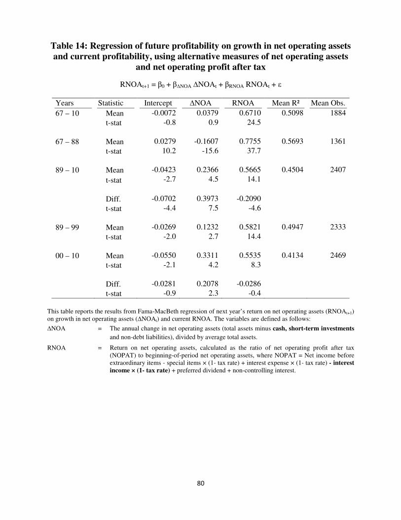
80
Table 14: Regression of future profitability on growth in net operating assets
and current profitability, using alternative measures of net operating assets
and net operating profit after tax
RNOAt+1 = β0 + β∆NOA ∆NOAt + βRNOA RNOAt + ε
Years Statistic Intercept ∆NOA RNOA Mean R² Mean Obs.
67 – 10 Mean -0.0072 0.0379 0.6710 0.5098 1884
t-stat -0.8 0.9 24.5
67 – 88 Mean 0.0279 -0.1607 0.7755 0.5693 1361
t-stat 10.2 -15.6 37.7
89 – 10 Mean -0.0423 0.2366 0.5665 0.4504 2407
t-stat -2.7 4.5 14.1
Diff. -0.0702 0.3973 -0.2090
t-stat -4.4 7.5 -4.6
89 – 99 Mean -0.0269 0.1232 0.5821 0.4947 2333
t-stat -2.0 2.7 14.4
00 – 10 Mean -0.0550 0.3311 0.5535 0.4134 2469
t-stat -2.1 4.2 8.3
Diff. -0.0281 0.2078 -0.0286
t-stat -0.9 2.3 -0.4
This table reports the results from Fama-MacBeth regression of next year’s return on net operating assets (RNOAt+1)
on growth in net operating assets (∆NOAt) and current RNOA. The variables are defined as follows:
∆NOA = The annual change in net operating assets (total assets minus cash, short-term investments
and non-debt liabilities), divided by average total assets.
RNOA = Return on net operating assets, calculated as the ratio of net operating profit after tax
(NOPAT) to beginning-of-period net operating assets, where NOPAT = Net income before
extraordinary items - special items × (1- tax rate) + interest expense × (1- tax rate) - interest
income × (1- tax rate) + preferred dividend + non-controlling interest.
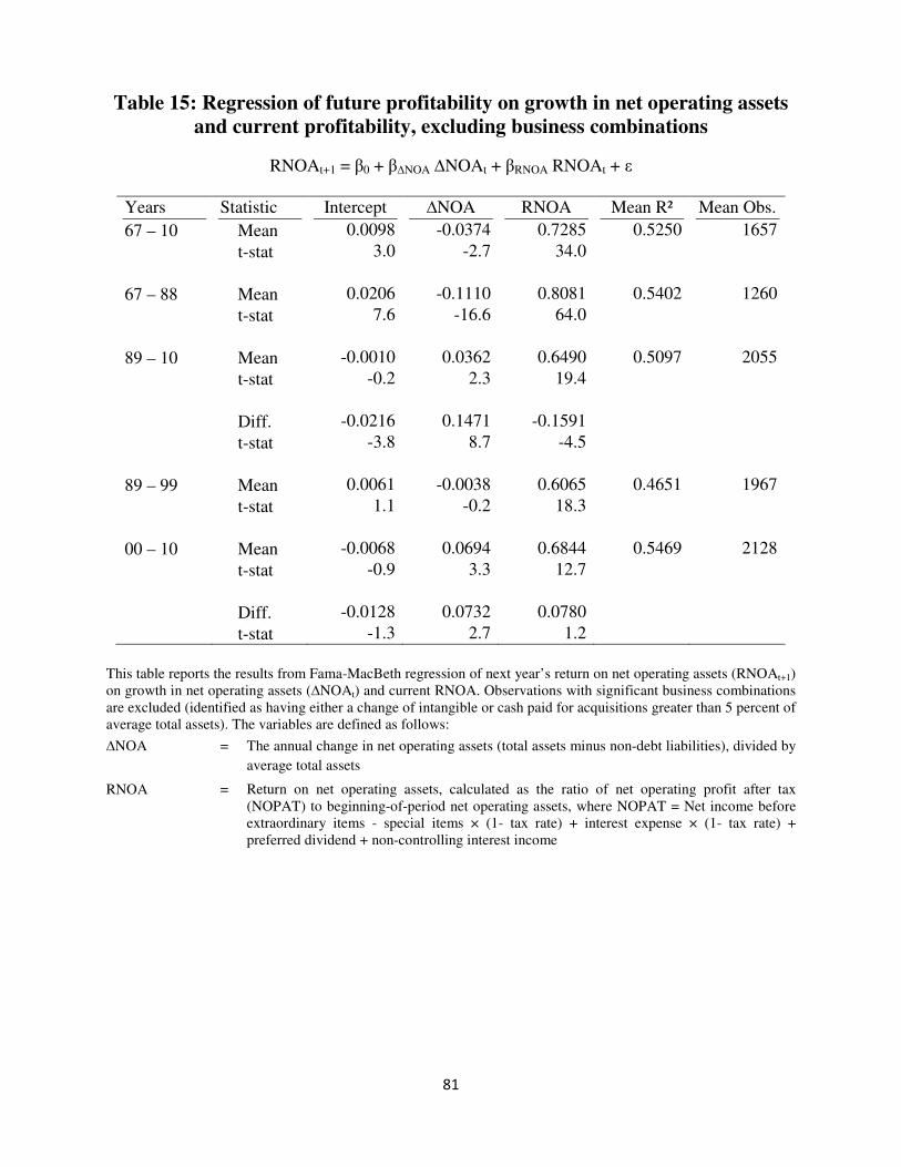
81
Table 15: Regression of future profitability on growth in net operating assets
and current profitability, excluding business combinations
RNOAt+1 = β0 + β∆NOA ∆NOAt + βRNOA RNOAt + ε
Years Statistic Intercept ∆NOA RNOA Mean R² Mean Obs.
67 – 10 Mean 0.0098 -0.0374 0.7285 0.5250 1657
t-stat 3.0 -2.7 34.0
67 – 88 Mean 0.0206 -0.1110 0.8081 0.5402 1260
t-stat 7.6 -16.6 64.0
89 – 10 Mean -0.0010 0.0362 0.6490 0.5097 2055
t-stat -0.2 2.3 19.4
Diff. -0.0216 0.1471 -0.1591
t-stat -3.8 8.7 -4.5
89 – 99 Mean 0.0061 -0.0038 0.6065 0.4651 1967
t-stat 1.1 -0.2 18.3
00 – 10 Mean -0.0068 0.0694 0.6844 0.5469 2128
t-stat -0.9 3.3 12.7
Diff. -0.0128 0.0732 0.0780
t-stat -1.3 2.7 1.2
This table reports the results from Fama-MacBeth regression of next year’s return on net operating assets (RNOAt+1)
on growth in net operating assets (∆NOAt) and current RNOA. Observations with significant business combinations
are excluded (identified as having either a change of intangible or cash paid for acquisitions greater than 5 percent of
average total assets). The variables are defined as follows:
∆NOA = The annual change in net operating assets (total assets minus non-debt liabilities), divided by
average total assets
RNOA = Return on net operating assets, calculated as the ratio of net operating profit after tax
(NOPAT) to beginning-of-period net operating assets, where NOPAT = Net income before
extraordinary items - special items × (1- tax rate) + interest expense × (1- tax rate) +
preferred dividend + non-controlling interest income
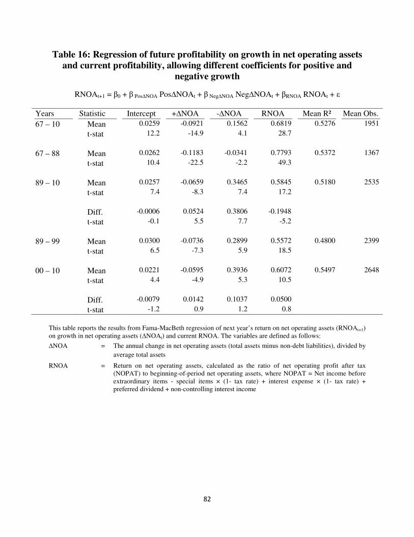
82
Table 16: Regression of future profitability on growth in net operating assets
and current profitability, allowing different coefficients for positive and
negative growth
RNOAt+1 = β0 + β Pos∆NOA Pos∆NOAt + β Neg∆NOA Neg∆NOAt + βRNOA RNOAt + ε
Years Statistic Intercept +∆NOA -∆NOA RNOA Mean R² Mean Obs.
67 – 10 Mean 0.0259 -0.0921 0.1562 0.6819 0.5276 1951
t-stat 12.2 -14.9 4.1 28.7
67 – 88 Mean 0.0262 -0.1183 -0.0341 0.7793 0.5372 1367
t-stat 10.4 -22.5 -2.2 49.3
89 – 10 Mean 0.0257 -0.0659 0.3465 0.5845 0.5180 2535
t-stat 7.4 -8.3 7.4 17.2
Diff. -0.0006 0.0524 0.3806 -0.1948
t-stat -0.1 5.5 7.7 -5.2
89 – 99 Mean 0.0300 -0.0736 0.2899 0.5572 0.4800 2399
t-stat 6.5 -7.3 5.9 18.5
00 – 10 Mean 0.0221 -0.0595 0.3936 0.6072 0.5497 2648
t-stat 4.4 -4.9 5.3 10.5
Diff. -0.0079 0.0142 0.1037 0.0500
t-stat -1.2 0.9 1.2 0.8
This table reports the results from Fama-MacBeth regression of next year’s return on net operating assets (RNOAt+1)
on growth in net operating assets (∆NOAt) and current RNOA. The variables are defined as follows:
∆NOA = The annual change in net operating assets (total assets minus non-debt liabilities), divided by
average total assets
RNOA = Return on net operating assets, calculated as the ratio of net operating profit after tax
(NOPAT) to beginning-of-period net operating assets, where NOPAT = Net income before
extraordinary items - special items × (1- tax rate) + interest expense × (1- tax rate) +
preferred dividend + non-controlling interest income
83
Appendix
Literature Review
This thesis builds on and contributes to several major strands of research, including the
accrual anomaly, the value relevance of earnings and book value, and behavioral explanations
for market anomalies. I review the related literature in turn with a focus on findings that are
relevant to my analysis. In some cases I discuss the same paper in multiple contexts.
1. The accrual anomaly
Accruals and the accrual anomaly
Accruals are utilized to mitigate the timing and matching problems of cash flows so that
earnings more closely reflect firm performance in continuous operation. Dechow (1994)
documents the benefits of accruals and establishes that earnings is a superior summary measure
of firm performance. She shows that: (1) over short measurement intervals, there is a stronger
contemporaneous association between stock returns and earnings than between stock returns and
realized cash flows; (2) as the measurement interval increases, the contemporaneous association
of stock returns with realized cash flows improves; (3) the advantage of earnings over cash flows
in explaining stock returns is particularly high among firms experiencing large changes in
working capital requirements, investments, and financing activities, i.e., when realized cash
flows have more severe timing and matching problems; (4) the longer a firm’s operating cycle,
the lower the contemporaneous association between stock returns and realized cash flows; (5)
long-term operating accruals play a less important role than working capital accruals in
mitigating timing and matching problems; and (6) special items reduce the earnings-return
association over short intervals.
84
While accruals generally mitigate the timing and matching problems of cash flows, they
are less persistent than cash flows. Sloan (1996) documents the accrual anomaly – the negative
relationship between accounting accruals and subsequent stock returns. Sloan hypothesizes that
investors naively fixate on bottom line income and fail to appreciate the different implications of
accruals and cash flows for future earnings. Firms with relatively high (low) level of accruals are
overvalued (undervalued). This mispricing is subsequently corrected when earnings are realized.
In support of this earnings fixation hypothesis, Sloan (1996) reports that about 40% of the
predictable stock returns are concentrated around the subsequent quarterly earnings
announcement dates.
Hribar and Collins (2002) assesses the error introduced by the indirect balance sheet
approach to accruals estimation. They argue that the balance sheet approach relies on the
presumed articulation between changes in balance sheet working capital accounts and the accrual
component of revenues and expenses on the income statement. This presumed articulation breaks
down when non-operating events such as reclassifications, mergers and acquisitions, divestitures,
accounting changes and foreign currency translations occur. Changes in current assets and
liabilities due to these non-operating events show up in the balance sheet, but do not flow
through the income statement. Consequently, a portion of the changes in balance sheet working
capital accounts relates to the non-operating events, and would erroneously be shown as accruals
under the balance sheet approach. Specifically, they show that mergers and acquisitions
introduce upward bias in balance sheet accruals, while discontinued operations induce a
downward bias. They find that the error induced by using a balance sheet approach contaminates
computations of discretionary or abnormal accruals, and can lead to erroneous conclusion that
earnings management exists when no such opportunistic activity is present. The errors-in-
85
variables problem may lead to the conclusion that there is no significant difference between the
pricing coefficients on accruals and cash flows, while the difference is significant using a cash
flow approach. Their final set of results indicate that measurement error from estimating accruals
using the balance sheet approach can bias tests of market mispricing of accruals towards zero
and lead to a null conclusion when significant mispricing exists.
Accruals and earnings quality
Sloan (1996) hypothesizes that the lower persistence of accruals is due to the subjectivity
involved in the estimation process and/or earnings management. Subsequent studies provide
evidence consistent with this hypothesis. Xie (2001) examines whether the market rationally
prices abnormal accruals estimated using the Jones (1991) model based on changes in sales
revenue and gross property, plant, and equipment. His results extend Sloan (1996) by suggesting
that the lower persistence and overpricing of total accruals reported by Sloan are due largely to
abnormal accruals.
Thomas and Zhang (2002) finds that the negative relation between accruals and future
abnormal returns is due mainly to inventory changes. They document several empirical
regularities for firms with extreme inventory changes, including (1) firms with inventory
increases (decreases) experience higher (lower) profitability, growth, and stock returns over the
prior five years, but those trends reverse after the extreme inventory change; (2) firms with
inventory increases (decreases) experience inventory decreases (increases) in the prior year, even
though profitability increases (decreases) in both years; (3) the abnormal returns observed after
the inventory changes are concentrated at subsequent quarterly earnings announcements and are
related to predictable earnings “surprises” reported at those announcements. They conjecture that
86
demand shifts cause the inventory change and related profitability reversal. They consider
earnings management and the impact of varying production levels on fixed manufacturing
overhead absorbed in COGS as potential reasons why the market does not fully recognize the
profitability reversals until the following year.
Richardson et al. (2005) investigates the relation between accrual reliability, earnings
persistence, and future stock returns. They assess the different degrees of reliability of different
categories of accruals and document that less reliable accruals lead to lower earnings persistence.
Investors seem to fail to anticipate the lower persistence of the less reliable accruals, which
results in a negative relation between accruals and future abnormal stock returns, with the
relation being stronger for less reliable accruals.
Dechow and Dichev (2002) suggests an approach to measure accruals quality as the
standard deviation of the residuals from firm-specific regressions of working capital accruals on
past, current, and one-year-ahead cash flows from operations, where higher standard deviation
denotes lower quality. They explore the relation between accruals quality and firm characteristics
including the length of operating cycle, firm size, sales volatility, cash flow volatility, accruals
volatility, earnings volatility, frequency of reporting negative earnings, and magnitude of
accruals. Accruals quality is positively related to earnings persistence.
Francis et al. (2005) investigates whether investors price accruals quality. They find that
poorer accruals quality is associated with larger costs of debt and equity. However, Core et al.
(2008) questions the validity of some of their findings.
The reversing nature of the accrual accounting hinders manager’s ability to make similar
biased estimates in continuous periods. When book value is already bloated as a result of
previous over-estimates, future profitability is likely to be depressed. Barton and Simko (2002)

87
argues that managers’ ability to optimistically bias earnings decreases with the extent to which
net assets are already overstated on the balance sheet relative to a neutral application of GAAP,
because net operating assets on balance sheet accumulates previous earnings management. They
demonstrate that the likelihood of reporting larger positive or smaller negative quarterly earnings
surprises decreases with the beginning balance of net operating assets relative to sales.
Hirshleifer et al. (2004) focuses on net operating assets as it is the cumulative difference
between net operating income and free cash flow. Net operating assets measure the extent to
which reporting outcomes provoke over-optimism. Hirshleifer et al. (2004) documents that net
operating assets scaled by total assets is a strong negative predictor of long-run future stock
returns. Net operating assets can be decomposed into the sum of cumulative operating accruals
(i.e., operating income before depreciation minus operating cash flow) and cumulative
investments (i.e., investment minus depreciation). Current period operating accruals, current
period investments, past periods’ operating accruals and investments all contribute to the ability
of NOA to predict future stock returns.
An inherent property of accrual accounting is that any accrual-based earnings
management in one period must reverse in another period. Dechow at el. (2012) shows that
incorporating priors concerning the timing of the reversal can significantly improve the power
and specification of tests for earnings management. Their results indicate that tests incorporating
reversals increase test power by around 40% and provide a robust solution for mitigating model
misspecification arising from correlated omitted variables.
88
Accruals, investment and growth
Fairfield et al. (2003a) extends the accrual anomaly by examining growth in net
operating assets, composed of both accruals and investment in long-term net operating assets.15
After controlling for current profitability, both components of ∆NOA – accruals and investment
in long-term net operating assets – have similar negative association with one-year-ahead return
on assets (ROA). They further demonstrate that the market appears to equivalently overprice
accruals and investment in long-term operating assets relative to their implications for one-year-
ahead ROA. The lower persistence of the accruals is therefore unlikely to be attributable to
managerial discretion. Instead, they suggest that diminishing marginal returns on investment
and/or conservative accounting practices contribute to the negative relation between growth in
net operating assets and future profitability.
In their follow-up paper, Fairfield et al. (2003b) notes that, in the literature related to the
differential persistence of accruals and cash flows, the dependent variable – future profitability –
is measured as one-year-ahead operating income (year t+1) divided by current invested capital
(year t). One-year-ahead profitability is affected not only by future income in the numerator
(income effect), but also by current growth in invested capital in the denominator (growth
effect). They hypothesize that the lower persistence of current operating accruals relative to cash
flows in explaining future profitability is due to the differential relation of these earnings
components with growth in invested capital which is the denominator of the profitability
measure. To isolate the effect of current ∆NOA (in year t) on future income, they deflate future
operating income by lagged NOA (year t-1) instead of current NOA and find that there is no
15
Sloan (1996) estimates accruals (noncash earnings) using changes in consecutive balance sheets. Hribar and
Collins (2002) points out that this measure of accruals also reflects non-operating events such as reclassifications,
mergers and acquisitions, divestitures, accounting changes and foreign currency translations. Thus, the stock-return
predictability of estimated accruals documented in Sloan (1996) may be partially due to balance sheet accruals.
89
differential persistence between accruals and cash flows after controlling for the effect of the
deflator. The lower persistence of accruals relative to cash flows is not attributable to a negative
association between accruals and one-year-ahead operating income but rather to the impact of
operating accruals on growth in net operating assets. They further suggest that the market
mispricing of accruals is due to investors’ inability to consider growth rates and the effects of
diminishing marginal returns and conservative accounting from new investment.
Penman and Zhang (2002) studies the effects of change in investment coupled with
conservative accounting on earnings quality. When the firm increases investment, conservative
accounting principles, which accelerate expense recognition and delay revenue recognition, lead
to lower reported earnings. Conversely, reducing investment or reducing the rate of investment
growth results in additional earnings. If the change in investment is temporary, current earnings
is temporarily depressed or inflated and is not a good indicator of future earnings. Penman and
Zhang (2002) constructs a C-score of inventory, R&D, and advertising reserves, measuring the
joint effects of investment and conservative accounting. They analyze how C-score predicts
changes in future return on net operating assets. The C-score is shown to forecast stock returns,
indicating that investors do not fully appreciate the impact of investments and accounting
conservatism on earnings quality.
Richardson et al. (2006) provides evidence on the role of temporary accounting
distortions in explaining the lower persistence of the accrual component of earnings. They
decompose the change in net operating assets into a growth component minus an efficiency
component. The growth component – sales growth – captures the diminishing marginal returns
on increased investment and/or accounting distortions in sales, while the efficiency component –
the rate of change in net operating asset turnover – is negatively related to temporary accounting
90
distortions. They find that the growth (efficiency) component is negatively (positively) correlated
with future profitability. Both working capital accruals and noncurrent operating accruals are
shown to be associated with SEC enforcement actions, suggesting that both components of
accruals are characterized by temporarily aggressive accounting distortions that are attributable
to managerial discretion.
Zhang (2007) studies two competing hypotheses for the accrual anomaly: accruals
capture low quality earnings (the persistence hypothesis), versus accruals reflect investment
(e.g., investment in working capital) that lead to lower stock return due to lower risk or
investors’ mispricing of past growth. Consistent with the investment hypothesis, Zhang finds that
(1) accruals co-vary strongly with growth attributes such as employee growth, external financing,
and cash sales growth, indicating that accruals capture fundamental investment information; (2)
the magnitude of the accrual anomaly monotonically increases with the investment information
contained in accruals, as measured by the co-variation between accruals and employee growth;
and (3) accruals show stronger (weaker) predictive power for future stock returns in industries
where accruals co-vary more (less) with employee growth.
Extending Zhang (2007), Wu et al. (2010) explores the risk-related investment
hypothesis of the accrual anomaly. Under this hypothesis, accruals measure investments, which
are related to changes in discount rates. Specifically, reductions in discount rates (expected
returns) lead to both larger investments (and hence accruals) and lower stock returns. Consistent
with this hypothesis, Wu et al. show that (1) accruals co-vary negatively with ex-ante one-year-
lagged discount rate estimated from both the dividend discount model and the residual income
model; (2) as accruals grow, future profitability and stock returns fall in accordance with
diminishing marginal returns to investment (firms accept projects of lower profitability at lower
91
required rate of return); (3) adding an investment factor into standard factor regression models
substantially attenuates the accrual anomaly; and (4) similar to the value/growth anomaly,
returns to accruals-based trading strategies are time-varying and countercyclical (high in bad
times and low in good times).16
Harris and Nissim (2006) suggests an alternative explanation on the negative relation
between growth in capital and subsequent stock return. Firms may grow earnings either by
improving the profitability of existing capital or by investing additional capital. Earnings growth
from incremental capital investment is less valuable than growth from improved profitability
because increases in capitals, unlike improvements in profitability, introduce incremental cost of
capital. Harris and Nissim (2006) shows that, in the long run, earnings growth due to increases in
invested capital is valued much less than growth resulting from improved profitability. In the
short run, however, investors overreact to earnings growth resulting from incremental capital
investment and underreact to earnings growth due to improved profitability; this mispricing is
subsequently corrected.
2. Value relevance of Earnings and Book Value
Extant research in accounting has demonstrated a decline in the value relevance of
earnings and a corresponding increase in the value relevance of book value over the past
decades. The literature has offered several explanations for the trends, including the impact of
changing firm characteristics, the increasing significance of real options, and a regulatory shift
from income statement approach to a balance sheet / fair value perspective. I start by reviewing
16
Specifically, Wu et al. show that the variance risk premium—the difference between implied and historical
volatility on the S&P 500 index which proxies for uncertainty and bad-versus-good times—predicts the returns to
accruals-based strategies with a significantly positive slope.
92
studies documenting the shift of the value relevance from earnings to book value, and then
discuss the explanations proposed for the shift.
The shift of value relevance from earnings to book value
Collins et al. (1997) finds that over the period 1953-1993 the combined value relevance
of earnings and book value, measured using R-squared from price-level regressions, has slightly
increased. While the incremental value relevance of earnings has declined, it has been replaced
by the increasing value relevance of book value. They attribute the shift in the value relevance
from earnings to book value to the increasing frequency and magnitude of one-time items, the
increasing frequency of negative earnings, the growing number of small firms, and the increasing
intangible intensity over time.
Lev and Zarowin (1999) documents that the cross-sectional association between stock
returns and reported earnings declines over the period 1978-1996. They argue that the increasing
rate of economic and operation changes and the ineffective accounting treatment of such changes
contribute to the temporal decline in the value relevance of earnings information. The weakening
of the return-earnings association is found to be more pronounced for firms whose R&D
intensity increases over the sample period than for firms with stable R&D.
Francis and Schipper (1999) examines the value relevance of financial accounting
information over the period 1952-1994. They show that returns to perfect foresight trading
strategies based on the sign and magnitude of earnings, on the level and change in earnings and
book value, and on an assortment of fundamental signals have decreased over the sample period.
However, returns based on cash flows and the sign of earnings have not changed significantly
over time. Using Easton and Harris’s (1991) model, Francis and Schipper find that the

93
explanatory power of earnings levels and earnings changes for stock returns has significantly
decreased over time. In contrast, the explanatory power of book value of assets and liabilities
(alone or combined with earnings) for market equity values has generally increased over time.
Economics Effects
To explain the decline in the incidence of dividend payers, Fama and French (2001a)
shows that the population of publicly traded firms tilts increasingly toward small firms with low
profitability and strong growth opportunities – characteristics typical of firms that have never
paid dividends. They also show that regardless of their characteristics, firms have become less
likely to pay dividends.
Kothari et al. (2002) compares future earnings variability, proxied with the standard
deviation of earnings levels or changes, generated from investment in R&D versus capital
expenditures. The future benefits from R&D expenditures are found to be more uncertain than
those from investment in capital expenditures. Book value takes on increased importance relative
to earnings when earnings are more volatile or negative.
Campbell et al. (2001) reports that stock return volatility increases dramatically over the
1962-1997 period, although aggregate market volatility does not change during this time period,
implying that the idiosyncratic risk of the typical stock has increased.
Comin and Mulani (2005) documents an increase in firm-level sales growth volatility,
in idiosyncratic return volatility, and in corporate bond spreads and ratings. They find that the
increase in firm volatility is associated with more competition in product markets, i.e., higher
turnover among industry leaders for both operating income and market value. Their evidence
94
supports that the increase in competition is linked to significant increase in R&D intensity and
significant increase in debt and equity issuance. Firm volatility also increases after deregulation.
Comin and Mulani (2006) documents that the growth rate of sales and employee at the
firm level have become more volatile while the growth rate of aggregate sales has become less
volatile, i.e., volatility at the aggregate and firm level following diverging trends. By
decomposing the variance, they show that the evolution of the volatility of aggregate growth rate
of sales is driven by the covariance of sales growth between firms, given the small magnitude of
the variance of firm sales. They propose to explain the diverging trend with innovations:
embodied innovations that lead to new products introduce firm-level volatility while the
individual gains and losses cancel each other at aggregate level; disembodied innovations
symmetrically affects all firms.
Irvine and Pontiff (2009) shows a significant increase over time in the idiosyncratic
volatility of firm-level earnings, cash flows, and sales, accompanying the increase in the
idiosyncratic return volatility over the same period. They rule out the possibility that the finding
can be explained entirely by higher proportions of smaller firms (by showing that the
fundamental idiosyncratic volatility also increases for large firms), changes in the composition of
industries (growing vs. contracting), new listings, or firms shifting towards focusing on fewer
lines of business. They propose to explain the increase in idiosyncratic risk over time with
increased competition in the economy. Their proxies for competition including ROA, industry
turnover, and market share from foreign competitors have a strong cross-sectional relation with
idiosyncratic return volatility, and also exhibit a time-series trend consistent with an increase in
competition. Deregulated industries (i.e., with increased competition) are found to experience
increased idiosyncratic risk. Examining cross-country evidence, they show that counties with
95
greater growth in idiosyncratic return volatility tend to have more competitive economies and
undergo faster change in technological innovation.
Accounting Effects
Accounting changes over the last three decades contribute to a shift in value relevance
from earnings to book value by (1) emphasizing conservative adjustments such as impairment
charges, (2) reducing the quality of matching in the income statement, and (3) increasingly
adjusting book value to reflect current condition.
Subramanyan and Wild (1996) shows that the informativeness of earnings is inversely
related to various characteristics that proxy for the likelihood that the firm will be terminated.
Basu (1997) interprets conservatism in accounting as earnings reflecting “bad news”
more quickly than “good news”. Using firms’ stock returns to measure news, Basu shows that
(1) the concurrent sensitivity of earnings to negative returns is two to six times as large as the
concurrent sensitivity of earnings to positive returns; (2) the greater timeliness of earnings
relative to cash flow is due primarily to more timely recognition of “bad news” through accruals,
and accruals do not improve the timeliness of recognizing “good news” in earnings; (3) positive
earnings changes tend to persist whereas negative earnings changes have a greater tendency to
reverse in the next period; (4) the association between positive earnings changes and
announcement period abnormal returns is stronger than negative earnings changes; and (5) the
sensitivity of earnings to concurrent negative returns increases relative to that of earnings to
concurrent positive returns over the last decades, suggesting that conservatism has increased over
time.
96
Please also refer to Lev and Zarowin (1999) discussed previously for empirical findings
regarding the decreased earnings’ value relevance and how it may result from the economic and
accounting changes.
Givoly and Hayn (2000) reports that firms’ profitability over the period 1950-1998 has
generally declined, but this decline is accompanied by a corresponding decline in cash flows.
Earnings distributions have become more dispersed and increasingly negatively skewed over
time. Long-term accruals have become significantly smaller and more volatile, and are the
greatest contributor to the increase in earnings variability. Another trend over the sample period
is the increasing significance of the more timely recognition of bad news relative to good news in
earnings.
Dichev and Tang (2008) provides empirical evidence supporting the conjecture that
matching becomes worse as a result of the evolution in accounting and the real economy over
time. They find a clear decrease in the correlation between contemporaneous revenues and
expenses and an increase in the non-contemporaneous correlation between revenues and
expenses. The volatility of reported earnings has doubled, while the underlying volatilities of
revenues and expenses have remained largely the same. There is a stark decline in the persistence
of earnings, and an increased negative autocorrelation in earnings changes. Additional analyses
show that the proliferation of one-time items and losses and changes in the real economy can
only explain some but not all of the results. The authors argue that accounting-based factors play
a substantial role in the temporal trends of earnings characteristics as the cash-based measures
reveal none of the temporal trends identified in accrual based results, and more pronounced
results are found for firms where the quality of accruals is low. The authors suggest that
97
standard-setters’ move towards a balance-sheet-based model of financial reporting has reduced
the forward-looking informativeness of earnings.
Building on Dichev and Tang (2008), Donelson et al. (2011) disaggregates total
expenses and finds that the decline in the contemporaneous association between revenues and
expenses over time (and the associated increase in earnings volatility and decrease in earnings
persistence) is primarily attributable to a steady increase in the frequency and magnitude of
special items. They construct an index (“E-Score”) of five indicator variables representing real
economic events that are likely to be associated with the most common special items, including
negative employee growth, merger and acquisition activity, discontinued operation, operating
loss, and negative sales growth. E-Score is shown to increase over time and is associated with the
cross-sectional probability of recording a special item. Targeted tests of specific special items
provide little evidence that the adoption of specific accounting standards affects the frequency of
the respective special items. Only for asset impairments, the implementation of SFAS 121
(effective in 1996) is found to be associated with an increase in special items, after controlling
for a general time trend and the E-Score. They also show that the changing incidence of
economic events is related to the well-documented increase in competition in the US economy.
Specifically, two indicators of competitive pressure, the Herfindahl Index and the Altman’s z-
score at industry level, are both increasing over time, and correlated with E-Score.
Elliott and Shaw (1988) studies the financial accounting performance and market returns
of firms taking asset write-downs during 1982-1985. They find that firms with large write-offs
substantially underperform their industries in the three years preceding and including the write-
off year (even after adding back the write-offs) in terms of return on assets and return on equity.
The declining performances in accounting terms are associated with significantly lower industry-
98
adjusted returns in periods three years before, event date, and 18 months following the
announcement of the write-offs. In addition, analysts’ current-year and year-ahead earnings
forecasts were reduced significantly after the announcement. Overall, their evidence suggests
that write-downs occur during a period of economic difficulties.
Elliott and Hanna (1996) shows a dramatic increase in the incidence of firms reporting
large special items. The increase in the frequency with which firms report negative special items
is up to three times higher than the incidence of reporting positive special items. More
importantly, they find that the information content of both “earnings before special items” and
“special items” is impaired when large special items are reported. The ability of unexpected
“earnings before special items” to explain security returns around earnings announcements for
firms associated with large write-offs is less than or equal to that for firms with no write-off. The
information content of “special items” measured at the earnings announcement date appears to
lessen as firms report longer sequences of large write-offs, i.e., repeated write-downs create
noise, which make it more difficult for the market to discern the true/recurring earnings of the
firm.
Black et al. (2000) reports that multiple occurrences of nonrecurring items such as
discontinued operations, special items, or extraordinary items, have a negative effect upon
market value of equity. They also find patterns of discretionary accruals consistent with
managers using special items to manage earnings upward prior to multiple write-downs. Firms
with multiple write-downs are more likely to go into liquidation or bankruptcy within the next
five years. Single occurrences also are value-relevant and are positively correlated with market
value.
99
Burgstahler et al. (2002) provides evidence confirming that special items are more
transitory than the remaining components of earnings. Their results suggest that positive special
items are largely transitory while negative special items are more of inter-period transfers, i.e.,
negative special items represent a shift of expense from future periods into the current period
(e.g., restructuring charges) that reduce current income but increase future income.
Dechow and Ge (2006) argues that high accruals are likely to be the outcome of rules
with an income statement perspective such as the booking of investment in working capital (e.g.,
inventory purchase) as assets to be matched against future revenue, while low accruals are likely
to be the outcome of rules with a balance sheet perspective such as impairment charges to mark
assets down to fair value. Consistent with this conjecture, Dechow and Ge show that for high
accruals firms earnings are more useful than cash flows for predicting future earnings, but for
low accrual firms cash flows are more useful. They also show that the low persistence of
earnings in low accrual firms is primarily driven by special items. Consistent with the hypothesis
that investors misunderstand the transitory nature of special items, low accrual firms with large
negative special items are found to earn higher positive stock returns than other low accrual
firms. Special item-low accrual firms perform very poorly in the special items year and there is
high uncertainty and pessimism regarding the prospects of these firms. Investors appear to
overweigh the probability that the firm will be unsuccessful: on average, the special item-low
accrual firms turn themselves around at higher rates than expected and so experience improved
stock price performance.
Barth (1994) studies a sample of U.S. banks and finds that fair value estimates of
investment securities provide significant explanatory power for equity value beyond that
provided by historical costs, while historical costs provide no significant explanatory power
100
incremental to fair values. Using a measurement error model, investment securities’ fair values
are found to have less measurement error than historical costs vis-à-vis the amount reflected in
share prices. Although fair value estimates of investment securities appear reliable and relevant
to investors in valuing bank equity, fair value securities gains and losses do not. Barth interprets
these findings as that although estimation error in the disclosed fair values is small enough that
investment securities’ fair values appear value-relevant, when two annual fair value estimates are
used to calculate securities gains and losses, the effect of combined estimation errors renders
securities gains and losses value-irrelevant.
Barth et al. (1995) finds that bank earnings calculated using fair value estimates of
investment securities gains and losses are significantly more volatile than that calculated using
historical cost securities gains and losses. However, this incremental volatility is not associated
with bank share prices, indicating that investors do not perceive fair value earnings volatility as a
better proxy for risk than historical cost earnings volatility. Banks would have violated
regulatory capital requirements more frequently had fair value accounting for investment
securities been used to calculate regulatory capital during the sample period. However, the
potential increase in regulatory risk associated with fair value accounting is not reflected in bank
share prices. Barth et al. also provide evidence that hypothetical fair violations are not
information events to the market but historical cost violations are. Changes in interest rates that
cause changes in fair value of investment securities are reflected in bank share prices.
Barth et al. (1998) shows that the explanatory power of book value for firm value is
significantly higher than that of net income for financial services firms. They argue that this is
because the book values of financial assets/liabilities, which comprise the majority of financial
institutions’ balance sheets, are recognized at amounts more closely approximating fair value.
101
Hann et al. (2007) studies the value- and credit-relevance of financial statements under
fair-value versus smoothing models of pension accounting. They show that fair-value pension
accounting introduces considerable volatility in net income, reducing its persistence and partially
obscuring the underlying information in operating income. Fair-value income is less value
relevant than smoothing income because of its lower persistence, and the fair value pension
obligation on balance sheet is marginally more value relevant. Their evidence suggests that the
fair value pension accounting model impairs the value- and credit-relevance of the combined
financial statements unless transitory gains and losses are separated from more persistent income
components. They find that the fair-value model improves (impairs) the credit relevance of
balance sheet (income statement) numbers.
Rees et al. (1996) documents that managers recognize asset impairments in years when
earnings are already low. They find significant negative abnormal accruals in the write-down
year, and these abnormal accruals do not tend to reverse and are generally close to zero in the
post-write-down years. They therefore suggest that the documented abnormal accruals in the
write-down year are due to permanent changes in the firms' accrual balances and managers are
responding to changes in economic circumstances as opposed to acting opportunistically. There
is a significantly positive association between abnormal accruals and contemporaneous stock
returns, which provides further support to the notion that managers' discretion provides important
information on firm value.
Bartov et al. (1998) investigates the informativeness of (i.e., long term stock price
performance before and after) the write-off announcements. Event date market reaction to the
write-off announcements shows clear difference between two types of write-offs (i.e., the “asset
write-down” category which comprises purely accounting decisions to reduce the carrying value
102
of assets with no apparent changes in operations, and the “operating decision” category). The
return to operating decision category is small and statistically insignificant, while the return to
the asset write-down firms is more than double that of the operating decision firms and highly
significant. Operating decisions convey two types of information that have opposite implications
for abnormal returns and offset each other: a lower value of firm book value and the plan for
improvements supposed to enhance future cash flows; asset write-downs convey bad news of
lower values of assets. Write-offs typically distort a firm’s earnings picture by packing large
losses into one quarter, thereby masking the trend underlying the firm’s earnings. Both types of
write-offs are preceded by large stock price declines, with a significantly bigger decline for the
asset write-down firms. The stock prices of both sets of write-off firms perform poorly during the
year following the announcement, but the asset write-down firms perform worse than the
operating decision firms.
Li et al. (2011) reports that investors and financial analysts revise downward their
expectations of value and earnings on the announcement of an impairment loss. In contrast, these
users of financial information do not revise their expectations on the announcement of zero
impairment by firms whose goodwill was previously considered to be potentially impaired.
Goodwill impairment serves as a leading indicator of a decline in future profitability. These
results suggest that the accounting pronouncements requiring the recognition of impairment
charges have improved the value relevance of book value.
Ayers (1998) compares the value relevance of deferred income taxes under the balance
sheet approach, mandated in the U.S. by SFAS 109 after 1992, with that under the income
statement approach of APB 11. SFAS No. 109 appears to increase the value relevance of
deferred tax amounts in financial statements. Specifically, Ayers shows that (1) SFAS No. 109
103
data represents value-relevant information above and beyond APB No. 11, and (2) the changes
made by SFAS No. 109 - the separate recognition of deferred tax assets, the creation of valuation
allowances for deferred tax assets, and the adjustment of deferred tax accounts for enacted tax
rate changes - each provide value-relevant firm data.
Amir et al (1997) finds that SFAS 109 deferred tax components arising from
depreciation and amortization, restructuring charges, environmental charges, employee benefit,
valuation allowance and other net deferred taxes are all value relevant for equity valuation.
Amir and Sougiannis (1999) examines how financial analysts and equity investors
incorporate information on deferred taxes from carry-forwards into earnings forecasts and share
prices. In providing this information each period, management must use their private information
about the firm’s profitability prospects, effectively providing a management earnings forecast.
They find a strong positive relation between deferred taxes from carry-forwards and share prices,
suggesting that these carry-forwards are valued as assets, and that the valuation allowance
required under SFAS 109 assists equity investors in valuing a firm's earnings and net assets.
Kumar and Visvanathan (2003) demonstrates that disclosures of changes in deferred
tax valuation allowances (VA) provide information beyond contemporaneous earnings reports.
Their evidence supports a characterization where investors use VA disclosures to infer
management's expectations about deferred tax assets, its realizability, and future taxable income
available for realization.
Real options
Hayn (1995) hypothesizes that because shareholders have a liquidation option, losses are
not expected to perpetuate and are less informative than profits about the firm’s future prospects.
104
The empirical results are consistent with the hypothesis: both the earnings response coefficient
and the information content of earnings as measured by � of the return-earnings regression are
depressed by the inclusion of loss cases; when the estimation sample consists only of loss cases,
the magnitude of reported losses does not appear to be related to the contemporaneous stock
price. Hayn also shows that the documented increase in the earnings response coefficient as the
cumulation period increases appears to be due exclusively to the effect of losses, i.e., the
likelihood of a cumulative loss declines with the cumulation period. The increase in the
frequency of losses over the years appears to partially explain the inter-temporal decline in the
earnings response coefficient and information content of earnings. The liquidation option effect
extends to profitable cases where earnings are low enough to make the option attractive. In
addition, the probability of losses is shown to be negatively related to firm size. Hayn proposes
that structural changes in the economy and changes in accounting principles with a greater
emphasis on mark-to-market accounting are two possible explanations to the observed increased
frequency of losses and the decline in the earnings response coefficient over the decades.
Burgstahler and Dichev (1997) develops an option-style model that values equity as a
convex function of both earnings and book value, where the function depends on the relative
value of earnings and book value. Earnings measure how the firm’s resources are currently used,
while book value measures the value of the firm’s existing resources. When the earnings/book
ratio is high, implying that the firm’s current activities are successful and are likely to be
continued, earnings are the primary determinant of equity value. When the earnings/book ratio is
low, the firm is more likely to exercise the option to adapt its resources to a superior alternative
use, and book value becomes the more important determinant of equity value. The empirical
evidence supports their prediction: the coefficient on earnings (book value) increases (decreases)
105
with the earnings/book ratio. The significance of these effects increases over the sample period
from 1976 to 1994.
Barth et al. (1998) hypothesizes that the value relevance of book value in explaining
firm value increases when a firm’s financial health deteriorates, because book value is a proxy
for liquidation value or the value of abandonment options; the value relevance of net income
declines when a firm’s financial health deteriorates, because the stream of future abnormal
earnings is likely to be relatively small in amount and short in duration. The empirical evidence
from both a sample of bankrupt firms and a large sample partitioned on bond ratings supports the
predictions.
Collins et al. (1999) demonstrates that the omission of book value of equity induces a
negative (positive) bias in the coefficient of earnings in the price-earnings relation for loss
(profit) firms, because book value is negatively (positively) correlated with profits for loss
(profit) firms while positively correlated with stock price. The coefficient on earnings is reliably
smaller for loss firms than for profit firms in every year, suggesting that the market views losses
as more transitory and places less weight on losses; the mean coefficient on book value does not
differ between profit and loss firms when aggregate bottom-line earnings are used, but
significantly larger for loss firms when core earnings and transitory components of current
earnings are used. Furthermore, they provide evidence on three competing hypotheses for the
role that book value of equity plays in valuing loss firms: (1) a control for scale difference, (2) a
proxy for expected future normal earnings, or (3) a proxy for loss firms’ abandonment
option. Their evidence does not support (1) but are consistent with (2) and (3).
Grullon et al. (2011) demonstrates that the positive relation between contemporaneous
firm-level stock returns and firm-level return volatility is due to firms’ real options. Consistent

106
with the real option theory, they find that the positive volatility-return relation is much stronger
for firms with more real options, whose value increases with volatility. They further show that
the sensitivity of firm value to changes in volatility declines significantly after firms exercise
their real options.
3. Market anomalies and the dynamics of investors’ reaction to financial information
The field of behavioral finance has seen an explosion of studies investigating behavioral-
based biases in investors’ reaction to information. Some anomalies—such as earnings
momentum and free cash flow anomaly—have been attributed to investors’ under-reaction to
relevant information; others including the value/growth and accruals anomaly have been
attributed to investors’ over-reaction.
Building on research in psychology that suggests that most people tend to overreact to
unexpected and dramatic news, DeBondt and Thaler (1985) demonstrates a similar behavior in
stock markets. They show that portfolios of prior “losers” outperform prior “winners,” and that
the large excess positive returns earned by the loser portfolio contribute significantly to the
January effect.
Fama and French (1992) finds that size and book-to-market equity capture the cross-
sectional variation in average stock returns associated with market beta, size, leverage, book-to-
market equity, and earnings-price ratios. Moreover, market beta is unrelated to average return
after controlling for size. Unlike most other studies of the value/glamour anomaly, Fama and
French argue that these strategies produce superior returns because they are fundamentally risky.
Lakonishok et al. (1994) provides evidence that value (or contrarian) strategies
outperform the market. Value strategies call for buying value stocks and selling glamour stocks,
107
where value stocks are underpriced stocks relative to their intrinsic value indicators such as book
value, earnings, cash flows or growth rate, and glamour stocks are overpriced stocks relative to
their intrinsic value indicators. Lakonishok et al. argue that the return differentials reflect a
correction of market mispricing caused by investors’ naive extrapolation of firms’ past sales or
earnings growth. In the long-run, stock prices drift towards intrinsic value, as proxied by the
fundamentals. They discuss that the return differential between glamour stocks and value stocks
is partially attributable to career concerns of portfolio managers, as glamour stocks appear to be
prudent investments and have lower career risk to portfolio managers compared to value stocks.
Consistent with the naïve extrapolation hypothesis, La Porta et al. (1997) finds that
approximately one third of the annual return differentials between value stocks and glamour
stocks is earned around earnings announcement dates. They also find that the return differential
between value stocks and glamour stocks is smaller in large stocks than in small stocks,
consistent with the notion that large stocks about which more information is available are less
susceptible to mispricing than small stocks. In contrast, Dechow and Sloan (1997) finds no
systematic evidence that stock prices reflect naive extrapolation of past trends in earnings and
sales growth. Instead, they find that stock prices appear to naively reflect analysts’ biased
forecasts of future earnings growth, and this naive reliance on analysts' forecasts of future
earnings growth can explain over half of the higher returns to contrarian investment strategies.