Causes of the EU ETS price drop: Recession, CDM, renewable policies ora bit of everything?—New evidence

Nicolas Koch a,n,1, Sabine Fuss a,b, Godefroy Grosjean c, Ottmar Edenhofer a,c,d

a Mercator Research Institute on Global Commons and Climate Change, Resources and International Trade, Torgauer Straße 12-15, 10829 Berlin, Germanyb International Institute for Applied Systems Analysis, Ecosystems Services & Management, Schlossplatz 1, 2361 Laxenburg, Austriac Potsdam Institute for Climate Impact Research, Telegrafenberg A31, 14473 Potsdam, Germanyd Technische Universität Berlin, Strasse des 17. Juni 135, 10623 Berlin, Germany

H I G H L I G H T S

� We examine whether abatement-related fundamentals justify the EU ETS price drop.� 90% of the variations of EUA price changes remain unexplained.� Variations in economic activity are robustly explaining EUA price dynamics.� Price impact of renewable deployment and international credit use remains moderate.� Reform options are evaluated in the light of the new findings.

a r t i c l e i n f o

Article history:Received 4 April 2014Received in revised form19 June 2014Accepted 20 June 2014Available online 11 July 2014

Keywords:EU ETSCarbon priceRenewables

a b s t r a c t

The price of EU allowances (EUAs) in the EU Emissions Trading Scheme (EU ETS) fell from almost 30€/tCO2 inmid-2008 to less than 5€/tCO2 in mid-2013. The sharp and persistent price decline has sparked intense debatesboth in academia and among policy-makers about the decisive allowance price drivers. In this paper weexamine whether and to what extent the EUA price drop can be justified by three commonly identifiedexplanatory factors: the economic recession, renewable policies and the use of international credits.Capitalizing on marginal abatement cost theory and a broadly extended data set, we find that only variationsin economic activity and the growth of wind and solar electricity production are robustly explaining EUA pricedynamics. Contrary to simulation-based analyses, our results point to moderate interaction effects between theoverlapping EU ETS and renewable policies. The bottom line, however, is that 90% of the variations of EUA pricechanges remains unexplained by the abatement-related fundamentals. Together, our findings do not supportthe widely-held view that negative demand shocks are the main cause of the weak carbon price signal. In viewof the new evidence, we evaluate the EU ETS reform options which are currently discussed.

& 2014 Elsevier Ltd. All rights reserved.

1. Introduction

The EU Emissions Trading Scheme (EU ETS), considered the flag-ship climate policy of the European Union, has experienced a sharpdecline in permit prices between 2008 and 2013. The price for EUAllowances (EUAs) went from 28€ per ton of carbon dioxide (tCO2) inmid-2008 to 5€/tCO2 at the time of writing this paper. Such depressedpermit prices are not likely to provide sufficient incentives for low-carbon technological investments (Nordhaus, 2011) and may increasethe risk of carbon lock-in (Clò et al., 2013). This situation has sparked

intense debates both in academia and among policy-makers about thereasons of the price drop, its impact on the effectiveness of the tradingscheme and options for reform (Clò et al., 2013; EuropeanCommission, 2012; Grosjean et al., 2014). To inform the debate, thispaper intends to investigate empirically the drivers of the current EUAprice movements with a special focus on overlapping climate policiesand the role of renewables in particular.

An extensive stream of the literature is devoted to exploringthe carbon pricing mechanism. Theory predicts that the permitprice should reflect market fundamentals related to the marginalcosts of emissions abatement; see e.g. Montgomery (1972) andRubin (1996),2. Fuel switching in the dominant power sector isconsidered to be the single most important abatement method in

Contents lists available at ScienceDirect

journal homepage: www.elsevier.com/locate/enpol

Energy Policy

http://dx.doi.org/10.1016/j.enpol.2014.06.0240301-4215/& 2014 Elsevier Ltd. All rights reserved.

n Corresponding author. Tel.: þ49 30 338 5537 231.E-mail address: koch@mcc-berlin.net (N. Koch).1 Postal address: Mercator Research Institute on Global Commons and Climate

Change, Torgauer Straße 12-15, 10829 Berlin, Germany. 2 For a recent survey of permit pricing theory, see Bertrand (2013).

Energy Policy 73 (2014) 676–685

the EU ETS (Delarue et al., 2008; Hintermann, 2010)3 and, conse-quently, in an efficient market, prices for input fuels are expected todetermine EUA prices. In addition, exogenous factors such as economicactivity or weather conditions are identified as relevant price funda-mentals, since they determine business-as-usual emissions, i.e. theneed for abatement (Hintermann, 2010). Empirical evidence relatingto these theoretical expectations is scattered over the differentregulatory periods which have been put in place in the EU ETS. Thepilot Phase I covered the period 2005 to 2007. Phase II coincided withthe Kyoto Protocol commitment period of 2008 to 2012. Phase III runsfrom 2013 to 2020. A series of studies empirically analyzes therelevance of the theoretically motivated price drivers in Phase I ofthe EU ETS (Aatola et al., 2013; Alberola et al., 2008a, 2008b;Chevallier, 2009; Hintermann, 2010; Mansanet-Bataller et al., 2007).The common finding is that the identified marginal abatement costdrivers had only a limited influence on EUA price formation. Evidencefor Phase II is relatively scarce and restricted to early Phase II (untilDecember 2010) when the EUA price was still around 15€/tCO2. Thefirst studies (Bredin and Muckley, 2011; Creti et al., 2012; Koch, 2014)suggest that a new pricing regime with an increased dependencybetween EUA, fuel and stock prices emerges in the Phase I-to-Phase IIperiod, which may be attributed to advances in the EU ETS marketdesign and maturity. Lutz et al. (2013) recently provide corroboratingevidence for the nonlinearity in the relation between EUA, energy andfinancial prices for the entire Phase II.

However, the economic environment as well as the policy envir-onment of the EU ETS has substantially changed since 2011. In fact, weknow very little about the causes of the EU ETS price drop over the lastthree years which ultimately led to the persistently low EUA pricelevel in 2013. The widely-held view among market participants,academics and policy-makers (Grosjean et al., 2014; de Perthuis andTrotignon, 2013) is that three main causes can be put forward toexplain the weak EUA price signal: (i) the deep and lasting economiccrisis in the European Union (Aldy and Stavins, 2012; EuropeanCommission, 2013; Neuhoff et al., 2012), (ii) the overlapping climatepolicies, e.g. feed-in tariffs for renewables (Fankhauser et al., 2010; Vanden Bergh et al., 2013; Weigt et al., 2013), and (iii) the large influx ofCertified Emission Reductions (CERs) and Emission Reduction Units(ERUs) in the EU ETS during Phase II (Neuhoff et al., 2012; Newell et al.,2012). However, an accurate assessment of the relative importance ofthe different explanatory factors is an outstanding empirical issue. Thisexamination is all the more important as Koop and Tole (2013) haveshown for the Phase I-to-Phase II period that there is substantialturbulence and change in the EU ETS pricing mechanism.

The economic crisis reduces the production of firms covered by theEU ETS, which decreases their demand for EUAs. Simultaneously, grimprospects of economic recovery reinforce the expectations of a lastinglow EUA demand, which affects the long-term price trend in thetrading scheme. Gloaguen and Alberola (2013) indeed find that theeconomic downturn plays a significant, but not dominant, role inthe decrease of CO2 emissions in EU ETS (see also Declercq et al., 2011).This finding suggests that other structural factors are also relevant forthe price formation.

Overlapping policies and more specifically the deployment ofrenewable energy sources (RES), have been cited as an additionalpossible explanation of the low EUA price. To reach the EU’s 20-20-20headline targets,4 EU Member States have launched generous supportmechanisms to stimulate RES deployment, which effectively contrib-uted to a marked expansion of wind and solar capacity in the

electricity sector (Edenhofer et al., 2013). The coexistence of EU ETSand RES deployment targets, however, creates a classic case ofinteraction effects (Goulder, 2013; Levinson, 2010). Theoretical workof Fankhauser et al. (2010) and Fischer and Preonas (2010) suggeststhat the overlapping policies work at cross-purposes, since RESinjections displace CO2 emissions within the EU ETS and therebyreduce the EUA demand and price.5 Corroborating the theory, severalsimulation-based studies predict that RES deployment exercises astrong downward pressure on EUA prices. For instance, simulations inVan den Bergh et al. (2013) suggest that RES deployment reduces theEUA price by 46€ in 2008 and more than 100€ in 2010. In thesimulation of De Jonghe et al. (2009) the allowance price could evendrop to zero depending on the stringency of targets (see also Ungerand Ahlgren, 2005; Weigt et al., 2013). However, Ellerman et al. (2014)highlight that it remains to be investigated whether the ex post effectof RES on the EUA price is large or small.

Finally, the unexpectedly high use of CERs/ERUs during Phase IIof the EU ETS might also contribute to a decreasing EUA demandand price. During the period 2008–2012, companies had alreadysurrendered for compliance more than 60% of the total permissible2008–2020 quota (Point Carbon, 2013). In particular, 2011 and2012 experienced a high use of Kyoto credits. This might beattributed to the collapse in credit prices (due to the non-ratification of the Kyoto protocol by major emitters) as well asthe European Commission’s change in the regulations regardingthe imports of credits from certain projects. More specifically, inPhase III credits originating from hydrofluorocarbon (HFC) andadipic acid nitrous oxide (N2O) projects are no longer permitted. Inaddition, new CERs are only allowed if they originate from least-developed countries (Kossoy and Guigon, 2012). As a consequence,companies surrendered for compliance large amounts of cheapcredits in the later years of Phase II. For instance, Berghmans andAlberola (2013) estimate that the power sector offsets around 65%of its shortfall of EUAs using Kyoto credits. In Phase III, however,the policy changes should rather reduce the number of availableCERs which may have a positive impact on the price of CERs ifdemand remains constant.

Our paper contributes to the literature by quantifying theactual impact of the different explanatory factors on the allowanceprice in EU ETS based on a broadly extended data set. A quanti-fication of the relative importance of the various price drivers isessential to understanding if and how the EU ETS should bereformed. We expand existing research by conducting a first expost analysis for the entire Phase II of the EU ETS and the first yearof Phase III (January 2008–October 2013). In particular, we applyextensive data on the deployment of intermittent RES, includingmonthly electricity production data for wind, solar and hydro-power that covers more than 80% of the (variable) renewableelectricity production in the European Union. The ex post data forRES allows us – for the first time – to investigate whether thecoexisting of EU ETS and RES targets work at cross-purposes.Previous research has focused on simulation-based modelingapproaches and, to the best of our knowledge, no empiricalanalysis has been carried out.

Our main findings are as follows: we detect a robust andstatistically significant – yet at the same time rather modest interms of magnitude – impact of intermittent renewables under-lining the importance of examining overlaps with other policies.Variations in economic activity are indeed the most important

3 This is due to (i) the ability of power generators to abate emissions withouteither cutting output or building new plants and (ii) the fact that the power andheat sector is dominant within the EU ETS (Kettner et al., 2008).

4 It is noteworthy that the legal status of the three goals varies: the GHGemissions reduction and RES share targets are binding while the energy efficiencytarget is indicative.

5 In theory, interactions could be mutual: the EU ETS could narrow the cost gapbetween RES technologies and conventional technologies and therefore stimulateRES deployment. This effect is, however, rather unlikely given the persistent lowEUA price level. For instance, Gavard (2012) shows that a carbon price of 46€ isnecessary to provide a price advantage to wind energy over electricity productionfrom gas.

N. Koch et al. / Energy Policy 73 (2014) 676–685 677

abatement-related determinant of EUA price dynamics. The Eco-nomic Sentiment Indicator is a particularly useful economic statevariable that is robustly explaining EUA price movements. Inaddition, we find a relatively small influence of CERs on EUA pricedynamics. However, this result could be biased due to the limita-tions of the publicly available CER data which requires us toassume that the number of issued CERs also reflects the numberof surrendered CERs in the EU ETS. In total, market fundamentalsexplain only a minor portion of the price decline in the EU ETSleading us to conclude that further analysis of different types ofdrivers is necessary. At the same time, reform options solelyadjusting the supply of EUA to economic activities or RES deploy-ment might not be a panacea. In fact, if a higher and more stableprice is seen as necessary to avoid lock-ins and promote long-termcost-effectiveness, it is doubtful that this can be achieved focusingonly on these drivers. From this point-of-view and depending onthe goals attached to the EU ETS, price instruments such as a pricecorridor might provide market participants with less uncertainty.Other approaches suggested entail delegation of governance, butthe feasibility of implementing this can be questioned (Grosjeanet al., 2014).

The paper is structured as follows. Section 2 provides detailedinformation on the data and methodology used. In Section 3, theresults are discussed, before the possible implications for the reformproposals are investigated in Section 4. Section 5 concludes.

2. Methods

2.1. Data

We consider monthly data for the sample period from January2008 until October, 2013. We have excluded Phase I data becausean extensive stream of the literature is already devoted toempirically ascertaining the EUA price drivers in Phase I of theEU ETS, while evidence for the Phase II-to-Phase III period remainsscarce.

2.1.1. EUA pricesWe rely on settlement prices of the year-ahead EUA December

futures contract traded on the ICE ECX platform to obtain a repre-sentative EUA price series. The price data is obtained from ICE FuturesEurope, the leading EU ETS trading venue. We rely on futures contractsrather than spot prices because the vast majority of EUA transactions(over 88% in 2011) are in futures (Kossoy and Guigon, 2012). Further,market microstructure analyses of Mizrach and Otsubo (2014) indicatethat the ICE ECX is providing between 75% and 88% of price discoveryfor EUA trading. December expiries are the most active contracts. It isnoteworthy, however, that both spot and futures prices may contributeinteractively to the dynamic process of price discovery in a nonlinearmanner, precisely because the relation between EUA spot and futuresprices is nonlinear (Arouri et al., 2012). Fig. 1 shows the EUA pricedevelopment over the sample period. In Phase II, the EUA priceinitially rises to almost 30€. With the financial crisis at the turn ofthe year 2008/09 the price decreases by about 50%. Then, after amoderate price recovery in early 2009, the price experiences a two-year period of remarkable stability around 15€. But mid-2011 the pricefalls again by around 50% to a new level of 7–8€ for 2012 before fallingto an even lower level of around 5€ with the start of Phase III.

2.1.2. Explanatory variablesAn extensive stream of the literature confirms the link between

EUA prices and fuel prices related to the abatement cost argumentdiscussed above (e.g., Alberola et al., 2008a; Creti et al., 2012;Hintermann, 2010; Mansanet-Bataller et al., 2007). Following thisliterature, we analyze the fuel switching price effect (i) implicitly by

including the gas and coal price and (ii) explicitly by calculating theswitching price. The latter indicates the theoretical carbon price whichmakes electricity producers indifferent between gas-fired and coal-fired generation. The price of gas is the month-ahead futures contractfor natural gas negotiated at the National Balancing Point (NBP). Weconsider this gas price from ICE Futures Europe, since it is the mostliquid gas trading point. For the coal price we rely on the month-aheadfutures contract of ICE Futures Europe which is priced against Argus/McCloskey’s API2 index with delivery to the Amsterdam–Rotterdam–

Antwerp (ARA) region. This price series is regarded as the primaryreference coal price for northwest Europe. We convert the gas price(from Pence/therm) and the coal price (from US$/t) into €/MWh usingexchange rates provided by the European Central Bank. Finally, thecalculated switching price is not only a function of gas and coal prices,but is also determined by the efficiency and emission rate of coal andgas plants in the EU ETS. The latter are taken from Delarue et al.(2010).6 Panel (a) of Fig. 1 shows the EUA price development on theone hand, and variations in the fuel (switching) prices on the otherhand. The most important feature is that there seems to be evidenceof a decoupling of the EUA price and the theoretical carbon switchingprice since 2011, making it unlikely that fuel switching may explainthe continued deterioration of EUA prices.

Economic activity is an important exogenous determinant ofbusiness-as-usual emissions and, therefore, EUA demand. To ascertainthe expected price effect, we use two forward-looking indicators ofeconomic activity. First, following the previous literature (e.g., Bredinand Muckley, 2011; Creti et al., 2012; Hintermann, 2010; Lutz et al.,2013), we rely on stock price movements as an indicator of currentand expected economic conditions. In addition, the inclusion ismotivated by the fact that it allows controlling for market disturbancessuch as the 2008/09 financial crisis. More specifically, we consider theSTOXX EUROPE 600 index, which is a broad benchmark index trackingthe performance in 18 European countries (Source: Thomson Data-stream).7 Second, we propose using the Economic Sentiment Indicator(ESI) published by Eurostat as alternative measure of economicconditions. This confidence indicator combines perceptions andexpectations about economic activity in the EU based on businesssurveys. We present the evolution of the two distinct economicvariables in Panel (b) of Fig. 1 jointly with the EUA price. In line withexpectations, the relatively strong co-movements of the time seriesindicate that economic activity may be an important explanatoryfactor of EUA prices. However, linkages are apparently weaker sincethe second half of 2012.

To account for potential trade-offs between the deployment ofelectricity from renewable energy sources (RES-E) and the carbonprice in an emissions trading regime, we include – for the first time –

an extensive data set of renewable energy deployment. The monthlyRES-E production data is obtained from the European Network ofTransmission System Operators for Electricity (ENTSO-E). The ENTSO-Edatabase provides power system data of all electric TransmissionSystem Operators (TSOs) in the EU in a standardized way. Two RES-Eproduction types are distinguished: first, hydro production, whichcomprises storage hydro, run of river and pumped storage; second,other RES-E production which compromises wind and solar.8 Data forthese two RES-E production variables in GWh is available for Austria,Belgium, France, Germany, Italy, Netherland, Portugal and Spain. Thesample accounts for 82% (44%) of total electricity production fromwind and solar (hydro) in EU ETS countries. The data coverage for

6 Coal burned at 36% efficiency: 951 tCO2/GWh; Gas burned at 50% efficiency:413 tCO2/GWh.

7 We choose a broad-based stock index (rather than a blue-chip index such asthe EURO STOXX 50) to ensure that any firm or sector-specific idiosyncrasies ingrowth prospects are smoothed out.

8 The inclusion of other RES such as biomass, landfill gas and biogases is notpossible because no reliable data is available for the entire period of analysis.

N. Koch et al. / Energy Policy 73 (2014) 676–685678

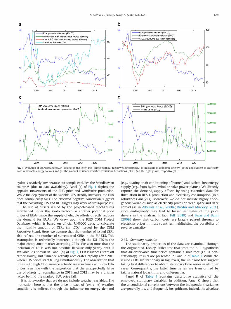
hydro is relatively low because our sample excludes the Scandinaviancountries (due to data availability). Panel (c) of Fig. 1 depicts theopposite movements of the EUA price and wind/solar production.While the deployment of the variable RES steadily increases, the EUAprice continuously falls. The observed negative correlation suggeststhat the coexisting ETS and RES targets may work at cross-purposes.

The use of offsets issued by the project-based mechanismsestablished under the Kyoto Protocol is another potential pricedriver of EUAs, since the supply of eligible offsets directly reducesthe demand for EUAs. We draw upon the IGES CDM ProjectDatabase, which is based on official UNFCCC data, to calculatethe monthly amount of CERs (in tCO2) issued by the CDMExecutive Board. Here, we assume that the number of issued CERsalso reflects the number of surrendered CERs in the EU ETS. Thisassumption is technically incorrect, although the EU ETS is themajor compliance market accepting CERs. We also note that theinclusion of ERUs was not possible because only yearly data isavailable. As shown in Panel (d) of Fig. 1, CER issuances start offrather slowly, but issuance activity accelerates rapidly after 2011when EUA prices start falling simultaneously. The observation thattimes with high CER issuance activity are also times with low EUAprices is in line with the suggestion that the unexpectedly largeuse of offsets for compliance in 2011 and 2012 may be a drivingfactor behind the marked EUA price fall.

It is noteworthy that we do not include weather variables. Themotivation here is that the price impact of (extreme) weatherconditions is indirect through the influence on energy demand

(e.g., heating or air conditioning of homes) and carbon-free energysupply (e.g., from hydro, wind or solar power plants). We directlycapture the demand/supply effects by using extended data forfluctuation in RES-E production and electricity consumption (in arobustness analysis). Moreover, we do not include highly endo-genous variables such as electricity prices or clean spark and darkspread (as in Alberola et al., 2008a; Bredin and Muckley, 2011),since endogeneity may lead to biased estimates of the pricedrivers in the analysis. In fact, Fell (2010) and Fezzi and Bunn(2009) show that carbon costs are largely passed through toelectricity prices in most countries, highlighting the possibility ofreverse causality.

2.1.3. Summary statisticsThe stationarity properties of the data are examined through

the Augmented–Dickey–Fuller test that tests the null hypothesisthat an observable time series contains a unit root (i.e. is non-stationary). Results are presented in Panel A of Table 1. While theissued CERs are stationary in log levels, the unit root test suggesttaking first differences to obtain stationary time series in all othercases. Consequently, the latter time series are transformed bytaking natural logarithms and differencing.

Panel B of Table 1 contains descriptive statistics of theemployed stationary variables. In addition, Panel C shows thatthe unconditional correlations between the independent variablesare generally low and frequently insignificant. Indeed, the absolute

Fig. 1. Evolution of EU Allowance (EUA) prices (on the left y-axis) jointly with (a) fuel (switching) prices, (b) indicators of economic activity, (c) the deployment of electricityfrom renewable energy sources and (d) the amount of issued Certified Emissions Reductions (CERs) (on the right y-axis, respectively).

N. Koch et al. / Energy Policy 73 (2014) 676–685 679

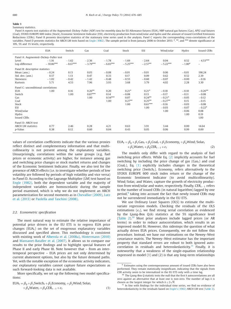
values of correlation coefficients indicate that the various proxiesreflect distinct and complementary information and that multi-collinearity is not present among the explanatory variables.Unsurprisingly, correlations within the same groups (e.g. fuelprices or economic activity) are higher, for instance among gasand switching price changes or stock market returns and changesof the Economic Sentiment Indicator. Finally, we also test for thepresence of ARCH effects (i.e. to investigate whether periods of lowvolatility are followed by periods of high volatility and vice versa)in Panel D. According to the Lagrange Multiplier (LM) test based onEngle (1982), both the dependent variable and the majority ofindependent variables are homoscedastic during the sampleperiod examined, which is why we do not implement an ARCHparameterization for second moments as in Chevallier (2009), Lutzet al. (2013) or Paolella and Taschini (2008).

2.2. Econometric specification

The most natural way to estimate the relative importance ofpotential price drivers in the EU ETS is to regress EUA pricechanges (EUAt) on the set of exogenous explanatory variablesdiscussed and specified above. This methodology is consistentwith existing work of Alberola et al. (2008a), Hintermann (2010)and Mansanet-Bataller et al. (2007). It allows us to compare ourresults to the prior findings and to highlight special features ofPhase II and early Phase III. Note however that – from an inter-temporal perspective – EUA prices are not only determined bycurrent abatement options, but also by the future demand paths.Yet, with the notable exception of the economic activity indicators,our explanatory variables cannot capture future expectations assuch forward-looking data is not available.

More specifically, we set up the following two model specifica-tions:

EUAt ¼ β0þβ1Switchtþβ2Economytþβ3Wind=Solartþβ4Watertþβ4CERt�1þεt ð1Þ

EUAt ¼ β0þβ1Gastþβ2Coaltþβ3Economytþβ4Wind=Solartþβ5Watertþβ6CERt�1þεt ð2Þ

The models only differ with regard to the analysis of fuelswitching price effects. While Eq. (2) implicitly accounts for fuelswitching by including the price change of gas (Gast) and coal(Coalt), Eq. (1) explicitly includes changes in the theoreticalswitching price (Switcht). Economyt refers alternatively to theSTOXX EUROPE 600 stock index return or the change of theEconomic Sentiment Indicator (to avoid multicollinearity).Wind=Solart and Watert capture the growth of electricity produc-tion fromwind/solar and water, respectively. Finally, CERt�1 refersto the number of issued CERs (in natural logarithm) lagged by oneperiod,9 taking into account the fact that newly issued CERs maynot be surrendered immediately in the EU ETS.

We use Ordinary Least Squares (OLS) to estimate the multi-variate regression models. Checking the residuals of the OLSestimations (εt), we find strong serial correlation as evidencedby the Ljung-Box Q ðkÞ statistics at the 5% significance level(Table 2).10 Most prior analyses include lagged prices (or ARterms) in order to reduce autocorrelation, which results in animproved model fit. However, this sidesteps the question of whatactually drives EUA prices. Consequently, we do not follow thisprocedure. Instead, we base our estimations on the Newey–Westcovariance matrix. The Newey–West estimator has the importantproperty that standard errors are robust to both ignored auto-correlation in residuals and heteroskedasticity.11 Finally, it isnoteworthy that a weakness of the single-equation relationshipexpressed in model (1) and (2) is that any long-term relationships

Table 1Summary statistics.

Panel A reports test statistics of the Augmented–Dickey–Fuller (ADF) test for monthly data for EU Allowance futures (EUA), NBP natural gas futures (Gas), API2 coal futures(Coal), STOXX EUROPE 600 index (Stock), Economic Sentiment Indicator (ESI), electricity production fromwind/solar and hydro and the amount of issued Certified EmissionsReductions (CERs). Panel B presents descriptive statistics of the stationary time series used in the analysis. Panel C reports the corresponding cross-correlations of thevariables. Panel D presents statistics for ARCH LM tests based on Engle (1982). The sample period is from January 2008 to October 2013. n, nn, and nnn denote significance at10%, 5% and 1% levels, respectively.

EUA Switch Gas Coal Stock ESI Wind/solar Hydro Issued CERs

Panel A: Augmented–Dickey–Fuller testLevel �1.16 �1.62 �2.36 �1.78 �1.69 �2.64 0.04 0.52 �4.53nnn

Log-difference �10.86nnn �8.67nnn �3.79nnn �6.83nnn �5.25nnn �2.57nn �5.22nnn �1.80n –

Panel B: descriptive statisticsMean (ann.) �0.24 0.13 0.03 �0.08 �0.01 �0.01 0.06 �0.01 198.24Std. dev. (ann.) 0.57 1.13 0.47 0.33 0.17 0.09 0.62 0.52 2.39Skewness �1.02 �0.42 �1.42 �0.48 �0.55 �0.60 �0.07 �0.00 �0.16Kurtosis 5.71 4.53 7.96 3.93 3.68 3.79 4.02 2.28 3.30

Panel C: unconditional correlationsEUA 1.00 0.16 0.26nn 0.20 0.21n 0.21n �0.18 �0.10 �0.26nn

Switch 1.00 0.87nnn 0.14 �0.08 0.13 �0.17 �0.11 �0.08Gas 1.00 0.54nnn 0.07 0.24nn �0.21n �0.05 �0.12Coal 1.00 0.27nn 0.25nn �0.27nn 0.15 �0.15Stock 1.00 0.61nnn �0.16 �0.03 �0.08ESI 1.00 �0.03 �0.07 �0.22n

Wind/solar 1.00 �0.06 0.08Hydro 1.00 0.19Issued CERs 1.00

Panel D: ARCH testARCH LM statistics 0.77 2.46 0.28 4.21 0.63 3.91 3.44 0.00 14.64p-Value 0.38 0.12 0.60 0.04 0.43 0.05 0.06 0.99 0.00

9 Estimates using the contemporaneous amount of issued CERs have also beenperformed. They remain statistically insignificant, indicating that the signals fromCER activity seem to be internalized in the EU ETS only with a time lag.

10 The Ljung-Box Q statistic tests the null that the first k autocorrelations are allzero against an alternative that at least one is non-zero. The number of lags k ischosen as the largest integer for which kr2

ffiffiffiffi

Np

.11 In line with findings for the individual time series, we find no evidence of

heteroskedasticity in the residuals based on Engle’s (1982) ARCH LM test (Table 2).

N. Koch et al. / Energy Policy 73 (2014) 676–685680

among EUA prices and their fundamentals cannot be estimated asinformation is lost due to differencing. Therefore, we also carry outcointegration analyses as robustness check.

3. Results

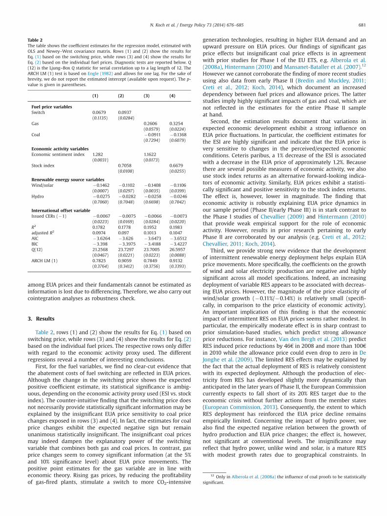
Table 2, rows (1) and (2) show the results for Eq. (1) based onswitching price, while rows (3) and (4) show the results for Eq. (2)based on the individual fuel prices. The respective rows only differwith regard to the economic activity proxy used. The differentregressions reveal a number of interesting conclusions.

First, for the fuel variables, we find no clear-cut evidence thatthe abatement costs of fuel switching are reflected in EUA prices.Although the change in the switching price shows the expectedpositive coefficient estimate, its statistical significance is ambig-uous, depending on the economic activity proxy used (ESI vs. stockindex). The counter-intuitive finding that the switching price doesnot necessarily provide statistically significant information may beexplained by the insignificant EUA price sensitivity to coal pricechanges exposed in rows (3) and (4). In fact, the estimates for coalprice changes exhibit the expected negative sign but remainunanimous statistically insignificant. The insignificant coal pricesmay indeed dampen the explanatory power of the switchingvariable that combines both gas and coal prices. In contrast, gasprice changes seem to convey significant information (at the 5%and 10% significance level) about EUA price movements. Thepositive point estimates for the gas variable are in line witheconomic theory. Rising gas prices, by reducing the profitabilityof gas-fired plants, stimulate a switch to more CO2-intensive

generation technologies, resulting in higher EUA demand and anupward pressure on EUA prices. Our findings of significant gasprice effects but insignificant coal price effects is in agreementwith prior studies for Phase I of the EU ETS, e.g. Alberola et al.(2008a), Hintermann (2010) and Mansanet-Bataller et al. (2007).12

However we cannot corroborate the finding of more recent studiesusing also data from early Phase II (Bredin and Muckley, 2011;Creti et al., 2012; Koch, 2014), which document an increaseddependency between fuel prices and allowance prices. The latterstudies imply highly significant impacts of gas and coal, which arenot reflected in the estimates for the entire Phase II sampleat hand.

Second, the estimation results document that variations inexpected economic development exhibit a strong influence onEUA price fluctuations. In particular, the coefficient estimates forthe ESI are highly significant and indicate that the EUA price isvery sensitive to changes in the perceived/expected economicconditions. Ceteris paribus, a 1% decrease of the ESI is associatedwith a decrease in the EUA price of approximately 1.2%. Becausethere are several possible measures of economic activity, we alsouse stock index returns as an alternative forward-looking indica-tors of economic activity. Similarly, EUA prices exhibit a statisti-cally significant and positive sensitivity to the stock index returns.The effect is, however, lower in magnitude. The finding thateconomic activity is robustly explaining EUA price dynamics inour sample period (Phase II/early Phase III) is in stark contrast tothe Phase I studies of Chevallier (2009) and Hintermann (2010)that provide weak empirical support for the role of economicactivity. However, results in prior research pertaining to earlyPhase II are corroborated by our analysis (e.g. Creti et al., 2012;Chevallier, 2011; Koch, 2014).

Third, we provide strong new evidence that the developmentof intermittent renewable energy deployment helps explain EUAprice movements. More specifically, the coefficients on the growthof wind and solar electricity production are negative and highlysignificant across all model specifications. Indeed, an increasingdeployment of variable RES appears to be associated with decreas-ing EUA prices. However, the magnitude of the price elasticity ofwind/solar growth (�0.11%/�0.14%) is relatively small (specifi-cally, in comparison to the price elasticity of economic activity).An important implication of this finding is that the economicimpact of intermittent RES on EUA prices seems rather modest. Inparticular, the empirically moderate effect is in sharp contrast toprior simulation-based studies, which predict strong allowanceprice reductions. For instance, Van den Bergh et al. (2013) predictRES induced price reductions by 46€ in 2008 and more than 100€in 2010 while the allowance price could even drop to zero in DeJonghe et al. (2009). The limited RES effects may be explained bythe fact that the actual deployment of RES is relatively consistentwith its expected deployment. Although the production of elec-tricity from RES has developed slightly more dynamically thananticipated in the later years of Phase II, the European Commissioncurrently expects to fall short of its 20% RES target due to theeconomic crisis without further actions from the member states(European Commission, 2013). Consequently, the extent to whichRES deployment has reinforced the EUA price decline remainsempirically limited. Concerning the impact of hydro power, wealso find the expected negative relation between the growth ofhydro production and EUA price changes; the effect is, however,not significant at conventional levels. The insignificance mayreflect that hydro power, unlike wind and solar, is a mature RESwith modest growth rates due to geographical constraints. In

Table 2The table shows the coefficient estimates for the regression model, estimated withOLS and Newey–West covariance matrix. Rows (1) and (2) show the results forEq. (1) based on the switching price, while rows (3) and (4) show the results forEq. (2) based on the individual fuel prices. Diagnostic tests are reported below. Q(12) is the Ljung–Box Q statistic for serial correlation up to a lag length of 12. TheARCH LM (1) test is based on Engle (1982) and allows for one lag. For the sake ofbrevity, we do not report the estimated intercept (available upon request). The p-value is given in parentheses.

(1) (2) (3) (4)

Fuel price variablesSwitch 0.0679 0.0937

(0.1135) (0.0284)Gas 0.2606 0.3254

(0.0579) (0.0224)Coal �0.0911 �0.1368

(0.7294) (0.6079)

Economic activity variablesEconomic sentiment index 1.282 1.1622

(0.0031) (0.0173)Stock index 0.7058 0.6679

(0.0108) (0.0255)

Renewable energy source variablesWind/solar �0.1462 �0.1102 �0.1408 �0.1106

(0.0007) (0.0297) (0.0035) (0.0399)Hydro �0.0275 �0.0282 �0.0258 �0.0246

(0.7060) (0.7048) (0.6698) (0.7042)

International offset variableIssued CERs (�1) �0.0067 �0.0075 �0.0066 �0.0073

(0.0223) (0.0169) (0.0284) (0.0220)R2 0.1782 0.1778 0.1952 0.1983adjusted R2 0.0974 0.097 0.1013 0.1047AIC �3.6264 �3.626 �3.6473 �3.6512BIC �3.398 �3.3975 �3.4188 �3.4227Q(12) 21.2568 23.7297 23.7005 26.5957

(0.0467) (0.0221) (0.0223) (0.0088)ARCH LM (1) 0.7825 0.9059 0.7849 0.9132

(0.3764) (0.3412) (0.3756) (0.3393)

12 Only in Alberola et al. (2008a) the influence of coal proofs to be statisticallysignificant.

N. Koch et al. / Energy Policy 73 (2014) 676–685 681

addition, our result is consistent with previous studies usingreservoir levels or perception as proxy for the supply of hydropower that turn out to have only marginal effects on EUA prices(Hintermann, 2010; Mansanet-Bataller et al., 2007).

Finally, we find a statistically significant negative influence ofthe issued CERs. However, given the tiny coefficient estimate, theeconomic significance of CERs seems rather limited. This findingmay imply that, contrary to expectations, the use of offsets has notnecessarily been a decisive factor impacting the EUA price.Specifically, the minor contribution from the Kyoto credits maybe explained on the basis that the maximum use of offsets wasanticipated when setting the cap. In fact, only the timing of offsetuse was different than expected because forward-looking marketparticipants adapted their offset imports to the changing regula-tion for international credits. However, we believe that theinterpretation of this result warrants some caution, since it couldbe attributed to the limitations of the available data. As outlinedabove, we have to assume that the number of issued CERs alsoreflects the number of surrendered CERs in the EU ETS. Obviously,this is technically incorrect and may introduce a bias. Moreover,the inclusion of ERUs was not possible because only yearly data isavailable. Although we acknowledge these limitations, weincluded the CER data in the analysis, in particular, to control foreffects of the unexpectedly large CER use in 2011 and 2012discussed above. It is noteworthy that all other estimates remainqualitatively very similar if we exclude the CER data.

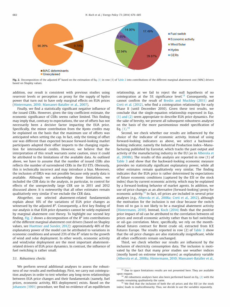
Altogether, our selected abatement-related fundamentalsexplain about 10% of the variations of EUA price changes aswitnessed by the adjusted R2. Consequently, a first key finding ofour analysis is that EUA price dynamics cannot be solely explainedby marginal abatement cost theory. To highlight our second keyfinding, Fig. 2 shows a decomposition of the R2 into contributionsof the different marginal abatement cost drivers (based on Shapleyvalues, see Huettner and Sunder, 2012): approximately 40% of theexplanatory power of the model can be attributed to variations ineconomic conditions and around 23% of the R2 relate to the growthof wind and solar deployment. In other words, economic activityand wind/solar deployment are the most important abatement-related drivers of EUA price dynamics. In contrast, the influence offuel switching is rather small.

3.1. Robustness checks

We perform several additional analyses to assess the robust-ness of our results and methodology. First, we carry out cointegra-tion analyses in order to test whether any long-term relationshipsbetween EUA price changes and their fundamentals (namely, fuelprices, economic activity, RES deployment) exists. Based on theJohansen (1991) procedure, we find no evidence of an equilibrium

relationship, as we fail to reject the null hypothesis of nocointegration at the 5% significance level.13 Consequently, wecannot confirm the result of Bredin and Muckley (2011) andCreti et al. (2012), who find a cointegration relationship for earlyPhase II (until December 2010). Given these test results, weconclude that the single-equation relationship expressed in Eqs.(1) and (2) seem appropriate to describe EUA price dynamics. Forthe sake of brevity, we present all subsequent robustness analyseson the basis of the more parsimonious model specification ofEq. (1).14

Second, we check whether our results are influenced by thechoice of the indicator of economic activity. Instead of usingforward-looking indicators as above, we select a backward-looking indicator, namely the Industrial Production Index—Manu-facturing published by Eurostat, which tracks the past output andactivity of the manufacturing industry in the EU (as in Alberola etal., 2008b). The results of this analysis are reported in row (1) ofTable 3 and show that the backward-looking economic measureprovides no statistically significant explanatory power, while allother estimates remain qualitatively very similar. The findingindicates that the EUA price is rather determined by expectationsof future economic conditions (captured by the ESI or the stockindex) than by current economic activity, which may be explainedby a forward-looking behavior of market agents. In addition, weuse oil price changes as an alternative (forward-looking) proxy foreconomic activity.15 In fact, oil prices are included in several prioranalyses (e.g., Alberola et al., 2008a; Creti et al., 2012), althoughthe motivation for the inclusion is not clear because the switchfrom oil to gas is not likely to be a marginal abatement activity(Hintermann, 2010). Instead, Koch (2014) finds that the positiveprice impact of oil can be attributed to the correlation between oilprices and overall economic activity rather than to fuel switchingor oil–gas correlation. More, specifically, we rely on the month-ahead futures contract for Brent crude oil, extracted from ICEFutures Europe. The results reported in row (2) of Table 3 showthat the oil price changes are also statistically insignificant, whileall other coefficients remain unchanged.

Third, we check whether our results are influenced by theinclusion of electricity consumption data. The inclusion is moti-vated by the fact that many prior studies use weather indices(mostly based on extreme temperatures) as explanatory variable(Alberola et al., 2008a; Hintermann, 2010; Mansanet-Bataller et al.,

Fig. 2. Decomposition of the adjusted R2 based on the estimation of Eq. (1) in row (1) of Table 2 into contributions of the different marginal abatement cost (MAC) driversbased on Shapley values.

13 Due to space limitations results are not presented here. They are availableupon request.

14 All robustness analyses have also been performed based on Eq. (2) with theresults remaining qualitatively the same.

15 We find that the inclusion of both the oil prices and the ESI (or the stockindex) leads to multicollinearity. Thus, we decide to use the variables separately.

N. Koch et al. / Energy Policy 73 (2014) 676–685682

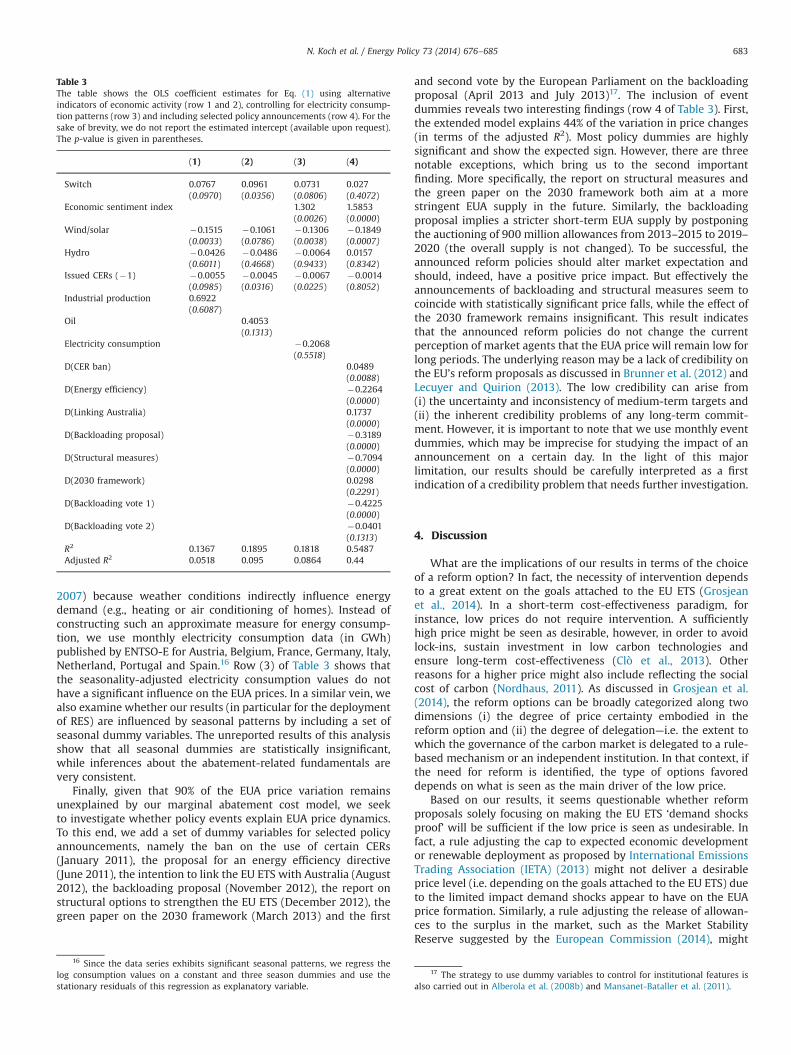
2007) because weather conditions indirectly influence energydemand (e.g., heating or air conditioning of homes). Instead ofconstructing such an approximate measure for energy consump-tion, we use monthly electricity consumption data (in GWh)published by ENTSO-E for Austria, Belgium, France, Germany, Italy,Netherland, Portugal and Spain.16 Row (3) of Table 3 shows thatthe seasonality-adjusted electricity consumption values do nothave a significant influence on the EUA prices. In a similar vein, wealso examine whether our results (in particular for the deploymentof RES) are influenced by seasonal patterns by including a set ofseasonal dummy variables. The unreported results of this analysisshow that all seasonal dummies are statistically insignificant,while inferences about the abatement-related fundamentals arevery consistent.

Finally, given that 90% of the EUA price variation remainsunexplained by our marginal abatement cost model, we seekto investigate whether policy events explain EUA price dynamics.To this end, we add a set of dummy variables for selected policyannouncements, namely the ban on the use of certain CERs(January 2011), the proposal for an energy efficiency directive(June 2011), the intention to link the EU ETS with Australia (August2012), the backloading proposal (November 2012), the report onstructural options to strengthen the EU ETS (December 2012), thegreen paper on the 2030 framework (March 2013) and the first

and second vote by the European Parliament on the backloadingproposal (April 2013 and July 2013)17. The inclusion of eventdummies reveals two interesting findings (row 4 of Table 3). First,the extended model explains 44% of the variation in price changes(in terms of the adjusted R2). Most policy dummies are highlysignificant and show the expected sign. However, there are threenotable exceptions, which bring us to the second importantfinding. More specifically, the report on structural measures andthe green paper on the 2030 framework both aim at a morestringent EUA supply in the future. Similarly, the backloadingproposal implies a stricter short-term EUA supply by postponingthe auctioning of 900 million allowances from 2013–2015 to 2019–2020 (the overall supply is not changed). To be successful, theannounced reform policies should alter market expectation andshould, indeed, have a positive price impact. But effectively theannouncements of backloading and structural measures seem tocoincide with statistically significant price falls, while the effect ofthe 2030 framework remains insignificant. This result indicatesthat the announced reform policies do not change the currentperception of market agents that the EUA price will remain low forlong periods. The underlying reason may be a lack of credibility onthe EU’s reform proposals as discussed in Brunner et al. (2012) andLecuyer and Quirion (2013). The low credibility can arise from(i) the uncertainty and inconsistency of medium-term targets and(ii) the inherent credibility problems of any long-term commit-ment. However, it is important to note that we use monthly eventdummies, which may be imprecise for studying the impact of anannouncement on a certain day. In the light of this majorlimitation, our results should be carefully interpreted as a firstindication of a credibility problem that needs further investigation.

4. Discussion

What are the implications of our results in terms of the choiceof a reform option? In fact, the necessity of intervention dependsto a great extent on the goals attached to the EU ETS (Grosjeanet al., 2014). In a short-term cost-effectiveness paradigm, forinstance, low prices do not require intervention. A sufficientlyhigh price might be seen as desirable, however, in order to avoidlock-ins, sustain investment in low carbon technologies andensure long-term cost-effectiveness (Clò et al., 2013). Otherreasons for a higher price might also include reflecting the socialcost of carbon (Nordhaus, 2011). As discussed in Grosjean et al.(2014), the reform options can be broadly categorized along twodimensions (i) the degree of price certainty embodied in thereform option and (ii) the degree of delegation—i.e. the extent towhich the governance of the carbon market is delegated to a rule-based mechanism or an independent institution. In that context, ifthe need for reform is identified, the type of options favoreddepends on what is seen as the main driver of the low price.

Based on our results, it seems questionable whether reformproposals solely focusing on making the EU ETS ‘demand shocksproof’ will be sufficient if the low price is seen as undesirable. Infact, a rule adjusting the cap to expected economic developmentor renewable deployment as proposed by International EmissionsTrading Association (IETA) (2013) might not deliver a desirableprice level (i.e. depending on the goals attached to the EU ETS) dueto the limited impact demand shocks appear to have on the EUAprice formation. Similarly, a rule adjusting the release of allowan-ces to the surplus in the market, such as the Market StabilityReserve suggested by the European Commission (2014), might

Table 3The table shows the OLS coefficient estimates for Eq. (1) using alternativeindicators of economic activity (row 1 and 2), controlling for electricity consump-tion patterns (row 3) and including selected policy announcements (row 4). For thesake of brevity, we do not report the estimated intercept (available upon request).The p-value is given in parentheses.

(1) (2) (3) (4)

Switch 0.0767 0.0961 0.0731 0.027(0.0970) (0.0356) (0.0806) (0.4072)

Economic sentiment index 1.302 1.5853(0.0026) (0.0000)

Wind/solar �0.1515 �0.1061 �0.1306 �0.1849(0.0033) (0.0786) (0.0038) (0.0007)

Hydro �0.0426 �0.0486 �0.0064 0.0157(0.6011) (0.4668) (0.9433) (0.8342)

Issued CERs (�1) �0.0055 �0.0045 �0.0067 �0.0014(0.0985) (0.0316) (0.0225) (0.8052)

Industrial production 0.6922(0.6087)

Oil 0.4053(0.1313)

Electricity consumption �0.2068(0.5518)

D(CER ban) 0.0489(0.0088)

D(Energy efficiency) �0.2264(0.0000)

D(Linking Australia) 0.1737(0.0000)

D(Backloading proposal) �0.3189(0.0000)

D(Structural measures) �0.7094(0.0000)

D(2030 framework) 0.0298(0.2291)

D(Backloading vote 1) �0.4225(0.0000)

D(Backloading vote 2) �0.0401(0.1313)

R2 0.1367 0.1895 0.1818 0.5487Adjusted R2 0.0518 0.095 0.0864 0.44

16 Since the data series exhibits significant seasonal patterns, we regress thelog consumption values on a constant and three season dummies and use thestationary residuals of this regression as explanatory variable.

17 The strategy to use dummy variables to control for institutional features isalso carried out in Alberola et al. (2008b) and Mansanet-Bataller et al. (2011).

N. Koch et al. / Energy Policy 73 (2014) 676–685 683

suffer from the same drawback. From such a perspective, a priceinstrument such as a price corridor or a price floor might offer abetter option to send a clear signal to market participants (Fell andMorgenstern 2009; Wood and Jotzo, 2011). A price floor can beimplemented as an auction reserve price in the EU ETS, i.e. anauction is only released when the auction price is beyond a pre-defined minimum price. In general, a price collar would generatethree potential market outcomes: (i) when EUA demand is low, theprice is set by the floor, and emissions are below the annual cap;(ii) when demand is moderate, the EUA price is somewherebetween the floor and ceiling, and the emissions are determinedby the cap; and (iii) when demand is high, the price is set by theceiling, and emissions are above the cap. Thus, the hybrid price-quantity mechanism would directly reduce the price uncertaintyin the EU ETS.

The policy-event dummies give us some evidence, althoughlimited, that regulatory uncertainty might play a role in price forma-tion. This finding, if confirmed, would imply different reform optionsthan the ones merely aimed at adjusting to short-term shocks (e.g. dueto economic downturn or large renewable deployment). Such reformoptions should seek to stabilize the expectations of market partici-pants. From this perspective, two types of approaches are discussed inthe literature: (i) reducing policy uncertainty and (ii) decreasing thelong-term commitment problem (Brunner et al., 2012). The formerinduces for instance the establishment of mid- to long-term legallybinding CO2 emissions reduction targets. The current debate isfocusing on the 2030 targets but to ensure long-term cost effective-ness, it might be necessary to provide to market participants a long-term decarbonization pathway. Nonetheless, as discussed in Grosjeanet al. (2014) such a strategy might not be sufficient to bring thenecessary level of stability to the expectations of market participants.

Tackling the long-term commitment problem in order to stabilizeexpectations is a delicate task. In monetary policy, the experience hasfavored delegation in setting the money supply as a tool to overcomethe problem (Barro and Gordon, 1983; Kydland and Prescott, 1977;Rogoff, 1985). In the context of the reform of the EU ETS, one couldforesee the delegation of the governance of the carbon market to anindependent authority whose goal would be to ensure that theshort-term EUA price is in line with long-term target (e.g. Clò et al.,2013; de Perthuis and Trotignon, 2013). However, this will not bewithout difficulties. The exact mandate of this institution as well asthe instrument used to achieve its goal will not be easily defined(Grosjean et al., 2014). Nonetheless, what an independent authoritymay achieve is a smoother decision-process for making reforms aswell as locating the decision outside of the political sphere (Newellet al., 2012). This might create more stable expectations on the waydecisions are taken over time, even if the goals are modified to adaptto new information and circumstances.

Based solely on the empirical findings discussed in this paper, itis difficult to assess exactly what type of reform is needed.However, it gives additional insight on the (limited) role ofabatement-related fundamentals on price development, in parti-cular with new results on the impact of renewables. In addition, itgives new evidence that regulatory uncertainty might negativelyimpact the EUA price, potentially undermining the ability of theEU ETS to deliver long-term cost-effectiveness. These are none-theless very preliminary findings and further research is neededto better understand the relation between regulatory uncertaintyand price formation as well as its influence on long-term cost-effectiveness.

5. Conclusion and policy implications

The price of EU allowances in the EU ETS fell from almost 30€in mid-2008 to less than 5€ in mid-2013. In this paper we look for

reasons behind the sharp and persistent decline of EUA prices inPhase II and early Phase III of the EU ETS. In particular, we examinewhether and to what extent the EUA price drop can be justified byabatement-related fundamentals derived from permit markettheory. Based on a broadly extended data set, we quantify theactual impact of three commonly identified explanatory factors ofthe low EUA price: the economic recession, renewable policies andthe use of international credits.

We find that EUA price dynamics cannot be solely explained bymarginal abatement cost theory. The set of abatement-relatedfundamentals explains only about 10% of the variations of EUAprice changes. Specifically, 40% of the explanatory power of themodel can be attributed to variations in expected economicconditions. Our results suggest that the Economic SentimentIndicator is a particularly useful economic state variable that isrobustly explaining EUA price movements. Consistent with the-ories suggesting that the coexistence of EU ETS and RES deploy-ment targets work at cross-purposes, we also find that the growthof wind and solar electricity production is a second importantdeterminant of EUA price drops. However, the estimated ex postsensitivity of EUA price changes to wind/solar growth is muchsmaller than predicted ex ante by simulation-based studies. Theimportant implication of this finding is that policy interactioneffects between ETS and RES targets are empirically moderate andpotentially exaggerated in simulation-based analyses. Finally, ourresults do not support the view that the large use of offsets isrelated to the EUA price fall. Although we find a statisticallysignificant negative influence of the issued CERs, the economicrelevance of CERs on EUA price dynamics seems rather limited.However, we stress again the potential bias in this result whichmay emerge from the necessary assumption that the number ofissued CERs also reflects the number of surrendered CERs in theEU ETS.

Given that 90% of the EUA price variation remains unexplainedby abatement-related fundamentals, it is necessary in furtherresearch to identify the true allowance price drivers. Although aconclusive answer to this question exceeds the scope of this paper,our robustness analysis suggests that policy events and a lack ofcredibility may be alternative explanations for the weak pricesignal. Indeed, a preliminary analysis of policy announcementeffects suggests that several announced reform policies apparentlydo not change the current perception of market agents that theEUA price will remain low for long periods. However, the use ofmonthly event dummies may be too imprecise for studying theimpact of policy events on market expectation and EUA prices. Webelieve that a key issue for future research is to verify whetherstructural weaknesses – and a lack of credibility in particular – areat the root of the inefficient carbon pricing mechanism. This iscrucial in order to structure the debate on the reform proposals forthe EU ETS, in particular in the framework of options delegating(at varying degrees) the governance of the EU ETS.

Acknowledgements

The authors would like to thank the participants of the Euro-CASE workshop in Brussels in February 2014 for their valuablefeedback and, in particular, Brigitte Knopf, Christian Flachslandand various colleagues at MCC and PIK for their constructivecomments on the study

References

Aatola, P., Ollikainen, M., Toppinen, A., 2013. Price determination in the EU ETSmarket: theory and econometric analysis with market fundamentals. EnergyEcon. 36, 380–395.

N. Koch et al. / Energy Policy 73 (2014) 676–685684

Aldy, J., Stavins, N., 2012. The promise and problems of pricing carbon: theory andexperience. J. Environ. Dev. 21 (2), 152–180.

Alberola, E., Chevalier, J., Chèze, B., 2008a. Price drivers and structural breaks inEuropean carbon prices 2005-07. Energy Policy 36 (2), 787–797.

Alberola, E., Chevalier, J., Chèze, B., 2008b. The EU emissions trading scheme: theeffects of industrial production and CO2 emissions on European carbon prices.Int. Econ. 116, 93–126.

Arouri, M., Jawadi, F., Nguyen, D.K., 2012. Nonlinearities in carbon spot-futures pricerelationships during Phase II of the EU ETS. Econ. Modelling 29, 884–892.

Barro, R.J., Gordon, D., 1983. A positive theory of monetary policy in a natural ratemodel. J. Polit. Econ. 91, 589–610.

Berghmans, N., E. Alberola, 2013. The Power Sector in Phase 2 of the EU ETS—FewerCarbon Emissions, but just as Much Coal. CDC Climate Report 42.

Bertrand, V., 2013. Modeling of Emission Allowance Markets: A Literature Review,Climate Economics Chair Working Paper 2013-04.

Bredin, D., Muckley, C., 2011. An emerging equilibrium in the EU emissions tradingscheme. Energy Econ. 33 (2), 353–362.

Brunner, S., Flachsland, C., Marschinski, R., 2012. Credible commitment in carbonpolicy. Clim. Policy 12 (2), 255–271.

Chevallier, J., 2009. Carbon futures and macroeconomic risk factors: a view fromthe EU ETS. Energy Econ. 31 (4), 614–625.

Chevallier, J., 2011. A model of carbon price interactions with macroeconomic andenergy dynamics. Energy Econ. 33, 1295–1312.

Clò, S., Battles, S., Zoppoli, P., 2013. Policy options to improve the effectiveness ofthe EU emissions trading system: a multi-criteria analysis. Energy Policy 57,477–490.

Creti, A., Jouvet, P.A., Mignon, V., 2012. Carbon price drivers: Phase I versus Phase IIequilibrium? Energy Econ. 34 (1), 327–334.

Declercq, B., Delarue, E., D’haeseleer, W., 2011. Impact of the economic recession onthe European power sector’s CO2 emissions. Energy Policy 39, 1677–1686.

Delarue, E., Voorspools, K., D’haeseleer, W., 2008. Fuel switching in the electricitysector under the EU ETS: review and prospective. J. Energy Eng.-ASCE 134,40–46.

Delarue, E., Ellerman, A.D., D’haeseleer, W., 2010. Robust MACCs? The topography ofabatement by fuel switching in the European power sector. Energy 35,1465–1475.

De Jonghe, C., Delarue, E., Belmans, R., D’haeseleer, W., 2009. Interactions betweenmeasures for the support of electricity from renewable energy sources and CO2

mitigation. Energy Policy 37, 4743–4752.Edenhofer, O., Hirth, L., Knopf, B., Pahle, M., Schlömer, S., Schmid, E., Ueckerdt, F.,

2013. On the economics of renewable energy sources. Energy Econ. 40, 12–23.Ellerman, A.D., Marcantonini, C., A. Zaklan, 2014. The EU ETS: Eight Years and

Counting. EUI Working Paper RSCAS 2014/04.Engle, R.F., 1982. Autoregressive conditional heteroskedasticity with estimates of

the variance of United Kingdom inflation. Econometrica 50, 987–1007.European Commission, 2012. The State of the European Carbon Market in 2012,

Report from the Commission to the European Council and Parliament, Brussels.European Commission, 2013. Green Paper. A 2030 Framework for Climate and

Energy Policies.European Commission, 2014. Proposal for a Decision of the European Parliament

and of the Council Concerning the Establishment and Operation of a MarketStability Reserve for the Union Greenhouse Gas Emission Trading Scheme andAmending Directive 2003/87/EC.

Fankhauser, S., Hepburn, C., Park, J., 2010. Combining multiple climate policyinstruments: how not to do it. Clim. Change Econ. 1 (3), 209–225.

Fell, H., 2010. EU-ETS and nordic electricity. Energy J. 31, 1–26.Fell, H., R. Morgenstern, 2009. Alternative Approaches to Cost Containment in a Cap-

and-Trade System, Resources for the Future Discussion Paper RFF DP 09-14.Fezzi, C., Bunn, D.W., 2009. Structural interactions of European carbon trading and

energy prices. J. Energy Markets 2, 53–69.Fischer, C., Preonas, L., 2010. Combining policies for renewable energy. Is the whole

less than the sum of its parts? Int. Rev. Environ. Resour. Econ. 4 (1), 51–92.Gavard, C., 2012. Carbon Price as Renewable Energy Support? Empirical Analysis on

Wind Power in Denmark. EUI Working Paper RSCAS 2012/19.Gloaguen, A., E. Alberola, 2013. Assessing the Factors behind CO2 Emissions

Changes Over the Phases 1 and 2 of the EU ETS: An Econometric Analysis.CDC Climate Research Working Paper 2013-15.

Goulder, L.H., 2013. Markets for pollution allowances: what are the (New) lessons?J. Econ. Perspect. 27 (1), 87–102.

Grosjean, G., Acworth, W., Flachsland, C., R. Marschinski, 2014. After MonetaryPolicy, Climate Policy: Is Delegation the Key to EU ETS Reform? MCC WorkingPaper, February 2014.

Hintermann, B., 2010. Allowance price drivers in the first phase of the EU ETS.J. Environ. Econ. Manage. 59, 43–56.

Huettner, F., Sunder, M., 2012. Axiomatic arguments for decomposing goodness offit according to Shapley and Owen values. Electron. J. Stat. 6, 1239–1250.

International Emissions Trading Association (IETA), 2013. Initial IETA Reflections onthe Concept of An “Automatic Adjustment of Auction Volumes” in the EU ETS.Retrieved from: ⟨http://www.ieta.org/assets/EUWG/ieta_reflection_flexible_supply_paper_02.10.2013_final.pdf⟩.

Johansen, S., 1991. Estimation and hypothesis testing of cointegration vectors inGaussian vector autoregressive models. Econometrica 59, 1551–1580.

Kettner, C., Köppl, A., Schleicher, S.P., Thenius, G., 2008. Stringency and distributionin the EU emissions trading scheme: first evidence. Clim. Policy 8, 41–61.

Koch, N., 2014. Dynamic linkages among carbon, energy and financial markets: asmooth transition approach. Appl. Econ. 46 (7), 715–729.

Koop, G., Tole, L., 2013. Forecasting the European carbon market. J. R. Stat. Soc. A 176(3), 723–741.

Kossoy, A., Guigon, P., 2012. States and Trends of the Carbon Market 2012. WorldBank.

Kydland, F., Prescott, E.C., 1977. Rules rather than discretion: the inconsistency ofoptimal paths. J. Polit. Econ. 85, 473–492.

Lecuyer, O., Quirion, P., 2013. Can uncertainty justify overlapping policy instru-ments to mitigate emissions? Ecol. Econ. 93, 177–191 (C).

Levinson, A., 2010. Belts and Suspenders: Interactions Among Climate PolicyRegulations. NBER Working Paper 16109.

Lutz, B.J., Pigorsch, U., Rotfuß, W., 2013. Nonlinearity in cap-and-trade systems: theEUA price and its fundamentals. Energy Econ. 40, 222–232.

Mansanet-Bataller, M., Pardo, A., Valor, E., 2007. CO2 prices, energy and weather.Energy J. 28, 73–92.

Mansanet-Bataller, M., Chevallier, J., Hervé-Mignucci, M., Alberola, E., 2011. EUAand sCER phase II price drivers: unveiling the reasons for the existence of theEUA–sCER spread. Energy Policy 39, 1056–1069.

Mizrach, B., Otsubo, Y., 2014. The market microstructure of the European climateexchange. J. Banking Finance 39, 107–116.

Montgomery, D.W., 1972. Markets in licenses and efficient pollution controlprograms. J. Econ. Theor. 5, 395–418.

Neuhoff, K., Schopp, A., Boyd, R., Stelmakh, K., Vasa, A., 2012. Banking of SurplusEmissions Allowances: Does the Volume Matter? DIW Discussion Papers 1193,1–21.

Newell, R.G., Pizer W.A., D. Raimi, 2012. Carbon Markets: Past, Present, and Future.NBER Working Paper 18504.

Nordhaus, W., 2011. Designing a friendly space for technological change to slowglobal warming. Energy Econ. 33, 665–673.

Paolella, M., Taschini, L., 2008. An econometric analysis of emission-allowanceprices. J. Banking Finance 32, 2022–2032.

de Perthuis, C., R. Trotignon, 2013. Governance of CO2 Markets: Lessons from the EUETS, Climate Economics Chair Working Paper 2013-07.

Point Carbon, 2013. Use of Credits for Compliance within EU ETS Nearly Doubles2012 Levels. Retrieved from: ⟨http://www.pointcarbon.com/aboutus/pressroom/pressreleases/1.2383916⟩.

Rogoff, K., 1985. The optimal degree of commitment to a monetary target. Q. J. Econ.100, 1169–1190.

Rubin, J.D., 1996. A model of intertemporal emission trading, banking, andborrowing. J. Environ. Econ. Manage. 31, 269–286.

Unger, T., Ahlgren, E.O., 2005. Impacts of a common green certificate market onelectricity and CO2-emission markets in the Nordic countries. Energy Policy 33,2152–2163.

Van den Bergh, K., Delarue, E., D’haeseleer, W., 2013. Impact of renewablesdeployment on the CO2 price and the CO2 emissions in the European electricitysector. Energy Policy 63, 1021–1031.

Weigt, H., Ellerman, A.D., Delarue, E., 2013. CO2 abatement from renewables in theGerman electricity sector: does a CO2 price help? Energy Econ. 40, 149–158.

Wood, P.J., Jotzo, F., 2011. Price floor for emissions trading. Energy Policy 39,1746–1753.

N. Koch et al. / Energy Policy 73 (2014) 676–685 685