case study - computational fluid dynamics (cfd) using ... · pdf fileintroduction case study...
TRANSCRIPT

IntroductionCase Study
Key Lessons
Case Study - Computational Fluid Dynamics(CFD) using Graphics Processing Units
Aaron F. Shinn
Mechanical Science and Engineering Dept., UIUC
Summer School 2009: Many-Core Processors for Science andEngineering Applications, 8-13-09
A.F. Shinn CFD using GPUs 1 / 30
IntroductionCase Study
Key Lessons
What is CFD?
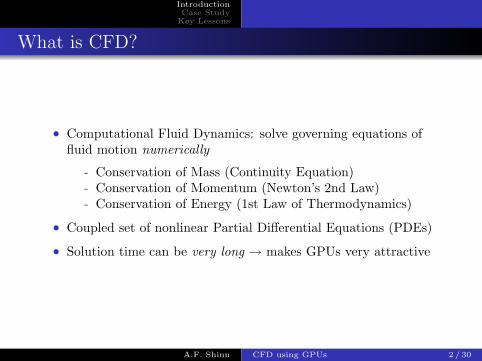
• Computational Fluid Dynamics: solve governing equations offluid motion numerically
- Conservation of Mass (Continuity Equation)- Conservation of Momentum (Newton’s 2nd Law)- Conservation of Energy (1st Law of Thermodynamics)
• Coupled set of nonlinear Partial Differential Equations (PDEs)
• Solution time can be very long → makes GPUs very attractive
A.F. Shinn CFD using GPUs 2 / 30

IntroductionCase Study
Key Lessons
General Governing Equations
Conservation of Mass∂ρ
∂t+∇ · ρu = 0
Conservation of Momentum
ρDuDt
= −∇p+∇ · ¯̄τ
Conservation of Energy
ρCpDT
Dt= βT
Dp
Dt+∇ · (k∇T ) + Φ
viscous stress tensor: ¯̄τ = µ(∂ui∂xj
+ ∂uj
∂xi
)+ δijλ(∇ · u)
substantial derivative: D( )Dt = ∂( )
∂t + u · ∇( )A.F. Shinn CFD using GPUs 3 / 30

IntroductionCase Study
Key Lessons
OverviewImplementationResults
Overview of Case Study
• Illustrate CFD implementation issues with “real” researchexample
• CU-FLOW: general-purpose Cartesian-based 3DNavier-Stokes solver written in C/CUDA for GPUs
• First implementation of fractional-step/multigridNavier-Stokes solver for Large-Eddy Simulations (LES) ofturbulence on GPUs
• Many different variations of this code were created• Countless hours spent on algorithm design, optimizations,
and debugging!
A.F. Shinn CFD using GPUs 4 / 30

IntroductionCase Study
Key Lessons
OverviewImplementationResults
Governing Equations for this Study
3D Incompressible Navier-Stokes equations
Conservation of Mass
∇ · u = 0
Conservation of Momentum∂u∂t
+ u · ∇u = −1ρ∇p+ ν∇2u
A.F. Shinn CFD using GPUs 5 / 30

IntroductionCase Study
Key Lessons
OverviewImplementationResults
Numerical Methodology
• Discretized via Finite-Volume Method on a staggeredCartesian mesh.
• Smagorinsky SGS model used for turbulence modeling.• Solved equations with fractional-step procedure.
- Pressure-Poisson equation (PPE) solved using red-blackGauss-Seidel.
- Geometric multigrid used for convergence acceleration ofPPE solution.
- Temporal advancement: explicit 2nd-orderAdams-Bashforth scheme.
- Spatial derivatives: 2nd-order central differencing.
A.F. Shinn CFD using GPUs 6 / 30

IntroductionCase Study
Key Lessons
OverviewImplementationResults
Geometric Multigrid: V-cycle
Figure: Multigrid V-cycle, where S=smooth, R=restrict residual,P=prolongate. Only three mesh levels are shown for simplicity.
A.F. Shinn CFD using GPUs 7 / 30

IntroductionCase Study
Key Lessons
OverviewImplementationResults
Multigrid: How good is it?
• Consider a unit square 2D domain, solve Laplace equation ∇2φ = 0 onthat domain
• Multigrid converges in just a few iterations, whereas using a singlegrid takes thousands!
Figure: Residuals of multigrid and single grid for solution of the Laplaceequation on a 256x256 grid, tolerance = 10−4.
A.F. Shinn CFD using GPUs 8 / 30

IntroductionCase Study
Key Lessons
OverviewImplementationResults
Layout of CU-FLOW code
Preprocessing on CPU
• set I.C. and B.C.
• generate mesh
• copy data to GPU
Time-stepping loop controlled on CPU
for(n=1; n<=nsteps; n++) {
Processing solution on GPU (call kernels)
• advance velocity from un to u∗ (Adams-Bashforth)
• advance pn to pn+1 (Multigrid V-cycle)
• advance u∗ to un+1
} // end time-stepping loop
Postprocessing on CPU
• copy data from GPU
• write plot files
A.F. Shinn CFD using GPUs 9 / 30
IntroductionCase Study
Key Lessons
OverviewImplementationResults
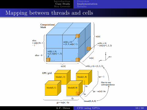
Mapping between threads and cells
Figure: Correspondence between GPU grid and computational mesh.A.F. Shinn CFD using GPUs 10 / 30

IntroductionCase Study
Key Lessons
OverviewImplementationResults
Multithreading Multigrid
• Optimal block size may conflict with mesh level dimensions.• Example: would like a 4x4x4 mesh as coarsest level, but
32x1x8 is optimal block size. Cannot map one-to-one dueto dimensions of block exceeding mesh.
• Question: how to resolve this conflict?• Possible solution: set block size based on mesh level.
A.F. Shinn CFD using GPUs 11 / 30

IntroductionCase Study
Key Lessons
OverviewImplementationResults
Multithreading Multigrid
Host code for calling a kernel
// define *fine mesh* dimensions of the blocks
#define bx_f 32
#define by_f 1
#define bz_f 8
// define *coarse mesh* dimensions of the blocks
#define bx_c 4
#define by_c 4
#define bz_c 4
...
for( n = 1; n<=ngrid; n++) {
// use block size for coarse mesh by default
bx = bx_c; by = by_c; bz = bz_c;
// for finer meshes, use better block size
if ( nx[n]%bx_f == 0 && ny[n]%by_f == 0 )
{ bx = bx_f; by = by_f; bz = bz_f; }
dim3 block(bx,by,bz);
dim3 grid(nx[n]/bx,ny[n]/by);
kernel<<<grid, block>>>(..., n, ...);
}
...
A.F. Shinn CFD using GPUs 12 / 30

IntroductionCase Study
Key Lessons
OverviewImplementationResults
Multithreading Multigrid
Device code for kernel__global__ void kernel(..., n, ...)
{
// i = tx + 2, j = ty + 2 (offset thread indices to mesh indices)
i = threadIdx.x + blockIdx.x * blockDim.x + 2;
j = threadIdx.y + blockIdx.y * blockDim.y + 2;
for (slice=0; slice<=nz[n]/blockDim.z-1; slice++)
{
k = threadIdx.z + slice * blockDim.z + 2;
m = i + (j-1)*(nx[n]+2) + \
(k-1)*(nx[n]+2)*(ny[n]+2) + begin[n] - 1;
... kernel computations ...
}
}
A.F. Shinn CFD using GPUs 13 / 30

IntroductionCase Study
Key Lessons
OverviewImplementationResults
CUDA implementation of Red-Black Gauss-Seidel
• Color the grid like a checkerboard to enable parallelprocessing of pressure
• First update the red pressures, then update the blackpressures
Figure: 2D example of red-black coloring of a mesh
A.F. Shinn CFD using GPUs 14 / 30
IntroductionCase Study
Key Lessons
OverviewImplementationResults
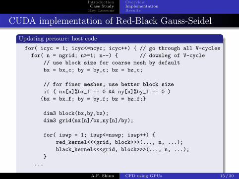
CUDA implementation of Red-Black Gauss-Seidel
Updating pressure: host code
for( icyc = 1; icyc<=ncyc; icyc++) { // go through all V-cycles
for( n = ngrid; n>=1; n--) { // downleg of V-cycle
// use block size for coarse mesh by default
bx = bx_c; by = by_c; bz = bz_c;
// for finer meshes, use better block size
if ( nx[n]%bx_f == 0 && ny[n]%by_f == 0 )
{bx = bx_f; by = by_f; bz = bz_f;}
dim3 block(bx,by,bz);
dim3 grid(nx[n]/bx,ny[n]/by);
for( iswp = 1; iswp<=nswp; iswp++) {
red_kernel<<<grid, block>>>(..., n, ...);
black_kernel<<<grid, block>>>(..., n, ...);
}
...
A.F. Shinn CFD using GPUs 15 / 30

IntroductionCase Study
Key Lessons
OverviewImplementationResults
CUDA implementation of Red-Black Gauss-Seidel
red kernel: device code
__global__ void red_kernel( ... ) {
i = threadIdx.x + blockIdx.x * blockDim.x + 2;
j = threadIdx.y + blockIdx.y * blockDim.y + 2;
for (slice=0; slice<=nz_d[n]/blockDim.z-1; slice++) {
k = threadIdx.z + slab * blockDim.z + 2;
if( (i+j+k)%2==0 ) { // test if red cell
m = i + (j-1)*(nx[n]+2)+(k-1)*(nx[n]+2)*(ny[n]+2)+begin[n]-1;
xm = xm[m]; xp = xp[m];
ym = ym[m]; yp = yp[m];
zm = zm[m]; zp = zp[m];
res = (aw_d[m] * pressure_d[xm] + ae_d[m] * pressure_d[xp] + \
as_d[m] * pressure_d[ym] + an_d[m] * pressure_d[yp] + \
al_d[m] * pressure_d[zm] + ah_d[m] * pressure_d[zp] + \
resc_d[m]) / ap_d[m];
pressure_d[m] = relxp*(res) + (1.0-relxp)*pressure_d[m];
} // end if
} //end slice
} //end kernel
A.F. Shinn CFD using GPUs 16 / 30

IntroductionCase Study
Key Lessons
OverviewImplementationResults
Profiling of CU-FLOW
• Red-black Gauss-Seidel kernels consume over 2/3 of GPUtime!
• Must optimize red-black Gauss-Seidel kernels
A.F. Shinn CFD using GPUs 17 / 30

IntroductionCase Study
Key Lessons
OverviewImplementationResults
CUDA implementation of Red-Black Gauss-Seidel
• Memory management in red-black kernels- Global memory: easiest, but slow- Shared memory: gives marginally better performance,
perhaps due to low data reuse or handling of boundaryhalos for each sub-domain in shared memory.
- Texture memory: fetch device memory through texturesinstead of expensive global memory load. Currently workingon this. This is an alternative to avoid uncoalesed memoryloads.
A.F. Shinn CFD using GPUs 18 / 30

IntroductionCase Study
Key Lessons
OverviewImplementationResults
Computational Resources
• GPU verison: CUDA, CPU version: Fortran.• Single-precision used for all calculations.• Dell Precision 690 Workstation (Linux: Red Hat Enterprise
5)• CPU: 3.0 GHz Intel Xeon• GPU: NVIDIA Tesla C1060 (∼ 1 teraFLOP)
A.F. Shinn CFD using GPUs 19 / 30

IntroductionCase Study
Key Lessons
OverviewImplementationResults
Laminar Flow in 3D Lid-Driven Cube
Figure: Computational domain for 3D lid-driven cube.
• ReL=1000• mesh: 128x128x128, constant mesh spacing.
A.F. Shinn CFD using GPUs 20 / 30

IntroductionCase Study
Key Lessons
OverviewImplementationResults
Laminar Flow in 3D Lid-Driven Cube
A.F. Shinn CFD using GPUs 21 / 30

IntroductionCase Study
Key Lessons
OverviewImplementationResults
Turbulent Flow in 3D square duct
Figure: Computational domain for 3D square duct.
• Reτ=360• mesh: 256x64x64, 3% geometric stretching in y-z plane.
A.F. Shinn CFD using GPUs 22 / 30
IntroductionCase Study
Key Lessons
OverviewImplementationResults
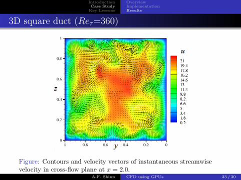
3D square duct (Reτ=360)
Figure: Contours and velocity vectors of instantaneous streamwisevelocity in cross-flow plane at x = 2.0.
A.F. Shinn CFD using GPUs 23 / 30

IntroductionCase Study
Key Lessons
OverviewImplementationResults
3D square duct (Reτ=360)
(a) present GPU simulation (b) Madabhushi and Vanka
Figure: Velocity vectors of mean flowfield in cross-flow plane.
A.F. Shinn CFD using GPUs 24 / 30

IntroductionCase Study
Key Lessons
OverviewImplementationResults
Speedup of GPU vs. CPU
• Performance of GPU versus CPU for first 100 time-steps ofsimulation, with block size bx=by=bz=4
Table 1: Laminar flow in lid-driven cube.
mesh Fortran code (sec) CUDA code (sec) speedup (CPU/GPU)
16x16x16 0.334 0.390 0.85632x32x32 3.082 1.236 2.49464x64x64 31.141 6.484 4.803
128x128x128 291.051 50.921 5.716
Table 2: Turbulent flow in a square duct.
mesh Fortran code (sec) CUDA code (sec) speedup (CPU/GPU)
256x64x64 208.088 34.555 6.022512x64x64 448.463 64.283 6.976
A.F. Shinn CFD using GPUs 25 / 30

IntroductionCase Study
Key Lessons
OverviewImplementationResults
Speedup of GPU vs. CPU
• Performance of GPU versus CPU for first 100 time-steps ofsimulation, with block size bx=by=bz=4 on coarser meshes andbx=32,by=1,bz=8 on finer meshes.
Table 1: Laminar flow in lid-driven cube
mesh Fortran code (sec) GPU code (sec) speedup (CPU/GPU)
16x16x16 0.334 0.307 1.0932x32x32 3.082 0.655 4.7164x64x64 31.141 2.710 11.49
128x128x128 291.051 18.349 15.86
Speedup improved by factor of 2.8 for 128x128x128 case
Table 2: Turbulent flow in square duct
mesh Fortran code (sec) GPU code (sec) speedup (CPU/GPU)
256x64x64 208.088 14.314 14.5
Speedup improved by factor of 2.4 for 256x64x64 case
A.F. Shinn CFD using GPUs 26 / 30

IntroductionCase Study
Key Lessons
Key Lessons
• Speedup of GPU scaled with the problem size; largestproblem size yielded maximum speedup.
• Single precision did not appreciably affect the results, evenfor turbulent flows.
• Global memory easiest to use, but worst for memorylatency.
• Need global residuals to observe convergence. This requirescudaMemcpy between CPU/GPU. Very expensive, so decidewhen you really need to see the residuals.
A.F. Shinn CFD using GPUs 27 / 30

IntroductionCase Study
Key Lessons
Key Lessons
• Optimization can be a time drain. Need to decide whencode is “good enough”
• Two possibilities:- Code is complete, just needs porting to CUDA and tuning.
Maybe have more time to optimize- Code is not complete, need to add physics features, write in
CUDA, and tune. Maybe need to spend more time onphysics algorithm and “get what you can get” out ofminimal time coding in CUDA
A.F. Shinn CFD using GPUs 28 / 30

IntroductionCase Study
Key Lessons
Future Work
• Model complex geometries in flow using the ImmersedBoundary Method (IBM)
• Multi-GPU capability - collaborating with John Stone,UIUC
A.F. Shinn CFD using GPUs 29 / 30

IntroductionCase Study
Key Lessons
References
[1] H. Ku, R. Hirsh, and T. Taylor. A Pseudospectral Method for Solution of theThree-Dimensional Incompressible Navier-Stokes Equations. Journal ofComputational Physics, 70:439-462, 1987.
[2] R.K. Madabhushi and S.P. Vanka. Large eddy simulation of turbulence-drivensecondary flow in a square duct. Phys. Fluids, 3(11):2734-2745, 1991.
A.F. Shinn CFD using GPUs 30 / 30