cascade flow calculations by a multigrid euler method flow calculations by a multigrid euler method...

JOURNAL OF PROPULSION AND POWERVol. 9, No. 1, Jan.-Feb. 1993

Cascade Flow Calculations by a Multigrid Euler Method

Feng Liu* and Antony JamesonfPrinceton University, Princeton, New Jersey 08544

An explicit finite-volume method for the Euler equations with multigrid is presented for calculating cascadeflows. The method is validated against theoretical test cases of the Hobson shock-free impulse cascade and asupersonic wedge cascade. Results for a VKI turbine cascade and a low-pressure turbine cascade are presentedand compared with experimental data. Isentropic Mach number distributions on blade surfaces show goodagreement with experiments at design conditions, whereas, discrepancy exists at off-design conditions due toflow separation. With equal efficiency the method is also able to capture qualitative features of secondary flowdue to inlet side-wall boundary layers.

Nomenclaturec = sound speedD = artificial dissipationE = stagnation energyE, F, G = flux vectors in the Euler equationsH = stagnation enthalpy(i> j, k) = grid point indicesk — summation indexP = forcing function in the multigrid methodp. = pressureq = total flow speedQ = flux balanceR = residual for the Euler equationsR = averaged residual for the Euler equationsS = entropy(u, v, w) = velocity components in x, y, z directionsVijk = cell volumeW = conserved flow variables in the Euler

equations(x, y, z) = Cartesian coordinates(a, j3, y) = inlet flow directional anglesaq = time-stepping coefficient for the qth stage of

the multistage time-stepping schemey = ratio of specific heatsAS = cell surface area8 = central difference operator, 8X(-) = (')i+l/2

- OX--1/2e = smoothing parameterp = densityfl = control volume

Subscriptsh, 2h = coarse and fine meshesi = interior cell valuesn = outer normal direction to a boundaryq = stages in the multistage time stepping00 = far-stream conditions

I. Introduction

I N order to take full advantage of computational fluid dy-namics in the design of turbomachinery blade rows, it is

Received March 23, 1992; revision received Sept. 11, 1992; ac-cepted for publication Sept. 17, 1992. Copyright © 1992 by F. Liuand A. Jameson. Published by the American Institute of Aeronauticsand Astronautics, Inc., with permission.

* Research Assistant; currently at Department of Mechanical andAerospace Engineering, University of California, Irvine, CA 92717.Member AIAA.

fProfessor, Department of Mechanical and Aerospace Engineer-ing. Fellow AIAA.

important to develop numerical methods that offer both ac-curate solutions for realistic flows and minimum computercost and turn-around time. While a three-dimensional Navier-Stokes solver is really needed for the above purpose, theproblem of turbulence modeling and the large amount ofcomputer time make a fast and robust three-dimensional Eu-ler solver still a desirable tool for routine applications. Fur-thermore, since the Euler equations do not preclude rota-tional flow, it is anticipated that, when proper inlet boundaryconditions are given and a fine enough mesh is provided, theEuler equations are capable of capturing features of secondaryflow vortices caused by the convection of the inlet side-wallboundary layers.

A notable Euler method for cascade-flow calculations wasdeveloped by Denton.1 The robustness, relative fast speed,and simplicity of the method earned its wide use in the tur-bomachine industry. On the other hand, a finite-volume methodwith a multiple stage time-stepping scheme proposed by Jame-son et al.2 has been very successful for external flows. Thismethod has the advantage of separated spatial and time dis-cretizations and is easy to implement. Coupled with a mul-tigrid scheme, the method can achieve computational effi-ciencies better than most other existing methods. Holmes3

first applied a four-stage version of the method without mul-tigrid to cascade calculations. Smith and Caughey4 later in-corporated multigrid and presented results for a rotor cascade.In this article we will present results with our latest versionof a five-stage cell-centered finite-volume method with mul-tigrids. The method is validated against theoretical test casesof the Hobson shockless impulse cascade and a supersonicwedge cascade. Detailed studies are carried out on a three-dimensional turbine cascade and the results are comparedwith those by Hodson and Dominy.5-7 One interesting featureof this work is that the method has been applied to calculatingrotational flow in an attempt to explore the possibility ofpredicting cascade secondary flow with an Euler code.

In the next section we will outline the basic numerical method.Section III describes the boundary conditions for typical cas-cade calculations. Section IV shows the results for the Hobsonimpulse cascade, a supersonic wedge cascade, and two turbinecascades. Comparisons of blade isentropic Mach number dis-tributions will be made between numerical calculation andexperiment. Preliminary results of secondary flow calculationswill also be presented to illustrate the capability and limita-tions of the inviscid calculation.

II. Numerical MethodA. Finite-Volume Scheme and Time Stepping

The basic numerical method is described in detail in Refs.8 and 9. For a perfect gasE = [pl(y - l)p] + \(u2 + v2 + w2), H = E + (pip)

90

LIU AND JAMESON: CASCADE FLOW CALCULATIONS 91

The Euler equations can be written in integral form as

~ L w dv

for a fixed region fl with boundary dft, where

W =

PpupvpwpE

pupuu + p

puvpuwpuH

F =

pvpuv

pw + ppvwpvH

s~i _

pwpuwpvw

pww + ppwH

The computational domain is divided into hexahedral cells.A system of ordinary differential equations can be obtainedby applying Eq. (1) to each cell and approximating the surfaceintegral with a finite-volume scheme

(2)

where Wijk is the average flow variable over the cell, Qijk isthe finite-volume approximation for the net flux out of thecell. With a cell-centered scheme Wijk is assumed to be at thecenter of the cell. Qijk can be evaluated as

(3)

Where Ek, Fk, and Gk denote values of the flux vectors E, F,and G on the kth face of the cell, (ASJ*, (&Sy)k, and (A^)*are the x, y, z components of the face area vector. Ek, Fk,and Gk can be evaluated by taking the averages of E, F, andG, respectively, on either side of the cell face.

The scheme constructed in this manner reduces to a central-difference scheme on Cartesian meshes, and is second-orderaccurate if the mesh is sufficiently smooth. To prevent oddand even decoupling and to capture shocks without oscilla-tions, an additional dissipation term is added to the semidis-crete Eq. (2) so that we solve

This is done in the following product form in three dimen-sions:

Rijk = Rij

Where ex, ey, and EZ are the smoothing parameters in eachdirection. Since it is only necessary to solve a sequence oftridiagonal equations for separate scalar variables, this schemerequires a relatively small amount of computational effort pertime step. Coupled with a multigrid scheme, the five-stagetime-stepping scheme with residual smoothing shows excellentconvergence rate. Although diagonalized fully implicit meth-ods are also available,10 the simplicity and applicability of themethod of residual smoothing for use on unstructured grids11

and parallel computing make it a desirable alternative.12

It can be shown for a one-dimensional model problem with-out dissipation that the scheme can be made stable for anyCourant number, provided the smoothing parameter is largeenough.8 In our calculation, best convergence is achieved atCourant numbers around nine with minimum smoothing. Inorder to further increase the rate of convergence, locally vary-ing time steps and enthalpy damping can also be used. Bothof these techniques are based on the assumption that thesolution approaches a steady state, and thus will not work fortime-accurate solutions.8'9

B. Multigrid MethodThe most effective method of accelerating convergence is

the multigrid method. Auxiliary meshes are introduced bydoubling the mesh spacing, and values of the flow variablesare transferred to a coarser grid by the rule

vhwh/v2

where the subscripts denote values of the mesh spacing pa-rameter. In three dimensions the sum is over the eight cellson the fine grid composing each cell on the coarse grid. Therule conserves mass, momentum, and energy. A forcing termis then defined as

= I

where R is the residual of the difference scheme. To updatethe solution on a coarse grid the multistage scheme is refor-mulated as

P2h)

(5)

+ RiJk(W) = 0 (4)

where Rijk is the residual

Rijk(W) = (HVijk)(Qijk - Dijk)

and Dijk is the artificial dissipation term which is formed in aconservative manner as a flux balance of blended first andthird differences of the flow variables in each coordinate di-rection.8

Equation (4) is then integrated in time by an explicit mul-tistage scheme. Multistage schemes are chosen because oftheir extended stability limit and high frequency dampingproperties which are appropriate for multigrid schemes. Forour calculations we have used a five-stage scheme with eval-uations of the dissipation term only at the first, third, andfifth stages. The readers are referred to Refs. 8 and 9 fordetails of the time-stepping scheme. The allowable Courantnumber for the five-stage scheme is 4.0. This number can befurther increased by smoothing the residuals at each stage.

where R(q} is the residual of the gth stage. In the first stageof the scheme, the addition of P2h cancels R2h[W(>Dt] and re-places it by S Rh(Wh), with the result that the evolution onthe coarse grid is driven by the residual on the fine grid. Thisprocess is repeated on successively coarser grids. Finally thecorrection calculated on each grid is passed back to the nextfiner grid by bilinear interpolation. In the present implemen-tation a W-cycle strategy12 is used in each time step.

Since the evolution on a coarse grid is driven by residualscollected from the next finer grid, the final solution on thefine grid is independent of the choice of dissipation andboundary conditions on the coarse grids when the computa-tion converges. To reduce the computational effort, only first-difference dissipation is used on the coarse grids. For externalflow calculations, some further reduction of computationaleffort can be achieved by freezing the far-field boundary con-ditions on the coarse grid calculations. It was found that, dueto the strong interactions of the inflow and outflow boundaryconditions with the interior flow in a cascade blade row, slowconvergence and possible limit cycles may be encountered ifthe inflow and outflow boundary conditions are not updated

92 LIU AND JAMESON: CASCADE FLOW CALCULATIONS

on each multigrid level as well as on the fine grid. In thecurrent work, the same boundary conditions discussed in thenext section are applied to all boundaries on all levels of thegrids.

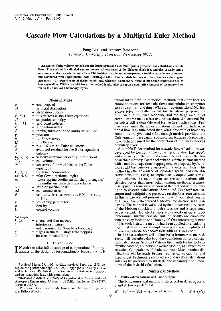
III. Boundary ConditionsAt present, H-type meshes are used. For cascade calcula-

tions we usually encounter four types of boundaries: 1) wall,2) periodic, 3) inlet, and 4) outlet as shown in Fig. 1. Imple-mentation of boundary conditions for a cell-centered finite-volume scheme is usually facilitated by using fictitious cellsexterior to the boundaries of the computational domain. Forwall boundaries, zero normal velocity is imposed, and we usethe normal momentum equation to extrapolate the pressureto the wall. For periodic boundaries, e.g., ab and AB in Fig.1, the flow variables in the fictitious cells below AB are madeto be the same as those in the interior cells right below ab,and the flow variables in the fictitious cells above ab are madeto be the same as those right above AB. Since a cell-centeredscheme is used, no special treatment is needed for the leadingand trailing edges of the blade profile.

At the inlet boundary, four of the five independent flowvariables must be specified for subsonic inlet flow. The otherflow variable must be extrapolated from inside the flowfieldaccording to characteristic analysis. For external flows, thefar-stream velocity is known since it is simply determined bythe flight speed. Therefore, we may specify a known velocitycomponent and let the flow angle be determined by the com-putation which should approach the undisturbed freestreamcondition if the boundary is far enough from the airfoil orwing. For cascade flows, usually the total pressure and totaltemperature (enthalpy) are given upstream. The velocity mag-nitude at the inlet, however, is determined by the back pres-sure downstream of the cascade. Different back pressuresresult in different velocities at the inlet. The flow angle, onthe other hand, does not change much even when the velocitymagnitude changes. In an experimental setup, e.g., the flowupstream comes from a stabilizing chamber where the flow isconditioned to be a nearly parallel stream entering the cascadeat a specific incidence angle. Specification of a velocity com-ponent is not a rational choice without knowing at least ap-proximately what the velocity magnitude is. If a rather ar-bitrary velocity component not consistent with the back pressureis chosen for the inlet, the resulting flowfield will then havea quite different incidence angle from the experimental con-dition. In light of the above argument we choose to specifythe total enthalpy, entropy, which is equivalent to total pres-sure, and the two independent flow angles of the incoming

flow. The one-dimensional Riemann invariant normal to theflow boundary is used to obtain the other condition. Let qnbe the velocity component in the direction of the outer normalof the inlet boundary and c the speed of sound for the fictitiouscells outside the inlet boundary, and let subscript / denote thecorresponding values on the interior cells adjacent to the inletboundary. The outgoing one-dimensional characteristic equa-tion can be written as

[2/(y - = qn + [2/(y - (6)

The conditions for the entropy, enthalpy, and flow angles canbe written as

S = S^ (7)

H = Hx (8)

(ulq) = cos a, (vlq) = cos /3, (w/q) = cos y (9)

where £«,, //TO, a, /3, and y are the given entropy, total en-thalpy, and the flow angles, a, /3, and y satisfy the followingcondition:

cos a2 + cos /32 + cos y2 = 1 (10)

Fig. 1 Computational domain and boundaries for typical cascadeswith an H grid.

With the above equations we can solve for all the flow vari-ables on the boundary, or rather, with the cell-centered schemeflow variables on the fictitious cells adjacent to the boundary.For supersonic inlet flow, all flow variables are specified.

Conversely on the outlet boundary, entropy, total enthalpyor the outgoing one-dimensional Riemann invariant, and flowangles are extrapolated for subsonic flow. In principle, anupstream running characteristic has to be used to reflect thefact of upstream influence in subsonic flows. However, in viewof experimental setup where the back pressure is controlledby a throttling device, here we choose to directly specify thepressure at the exit of the cascade. For outlet flow with super-sonic axial velocity all variables are extrapolated.

Because of the existence of the hub and casing in a three-dimensional cascade, the flow develops boundary layers overthe sidewalls before it enters the cascade blading where low-energy flow in the sidewall boundary layers undergoes thesame blade-to-blade pressure gradient as the inviscid coreflow. The interaction of these sidewall boundary layers withthe cascade blades results in secondary flow phenomena. Itappears that the essential vortical features of secondary flowsmay be determined by inviscid vortex dynamics which can bedescribed by the Euler equations provided a rotational ve-locity profile that include the sidewall boundary layers is spec-ified at the entrance of the cascade. This velocity profile canbe taken from experimental measurement or obtained by as-suming appropriate boundary-layer profiles with given mo-mentum and displacement thicknesses. The velocity profile isthen converted into an entropy or stagnation pressure profileby assuming a constant static pressure at the inlet boundary,and with a given stagnation enthalpy so that implementationof the inlet boundary conditions can be carried out in themanner described in the above paragraphs. It must be pointedout, however, that secondary flows are really of viscous origin,and therefore, the results of inviscid simulation ought to beappropriately interpreted.

IV. Computational Results

A. Hobson's Impulse CascadeOne of the most difficult test cases for transonic cascade

calculations is the Hobson shock-free impulse cascade.13 Ithas very thick airfoils and was designed with the hodographmethod to give a shock-free supersonic pocket. Since any suchshock-free solution is isolated in the sense that a small per-turbation in the flow conditions or airfoil shape can cause a


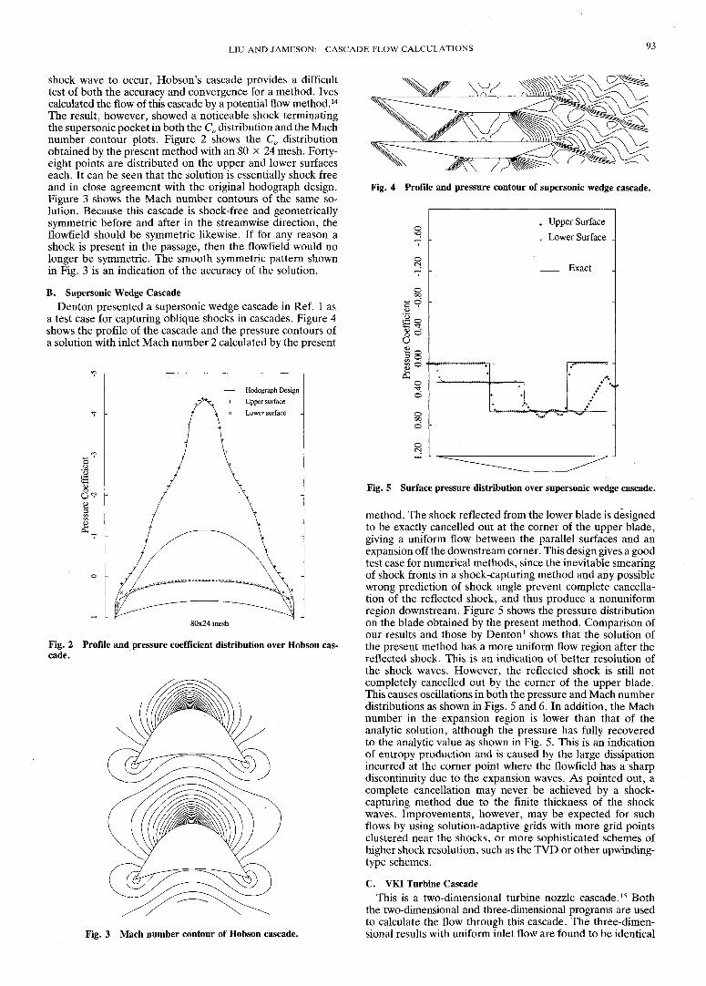
shock wave to occur, Hobson's cascade provides a difficulttest of both the accuracy and convergence for a method. Ivescalculated the flow of this cascade by a potential flow method.14

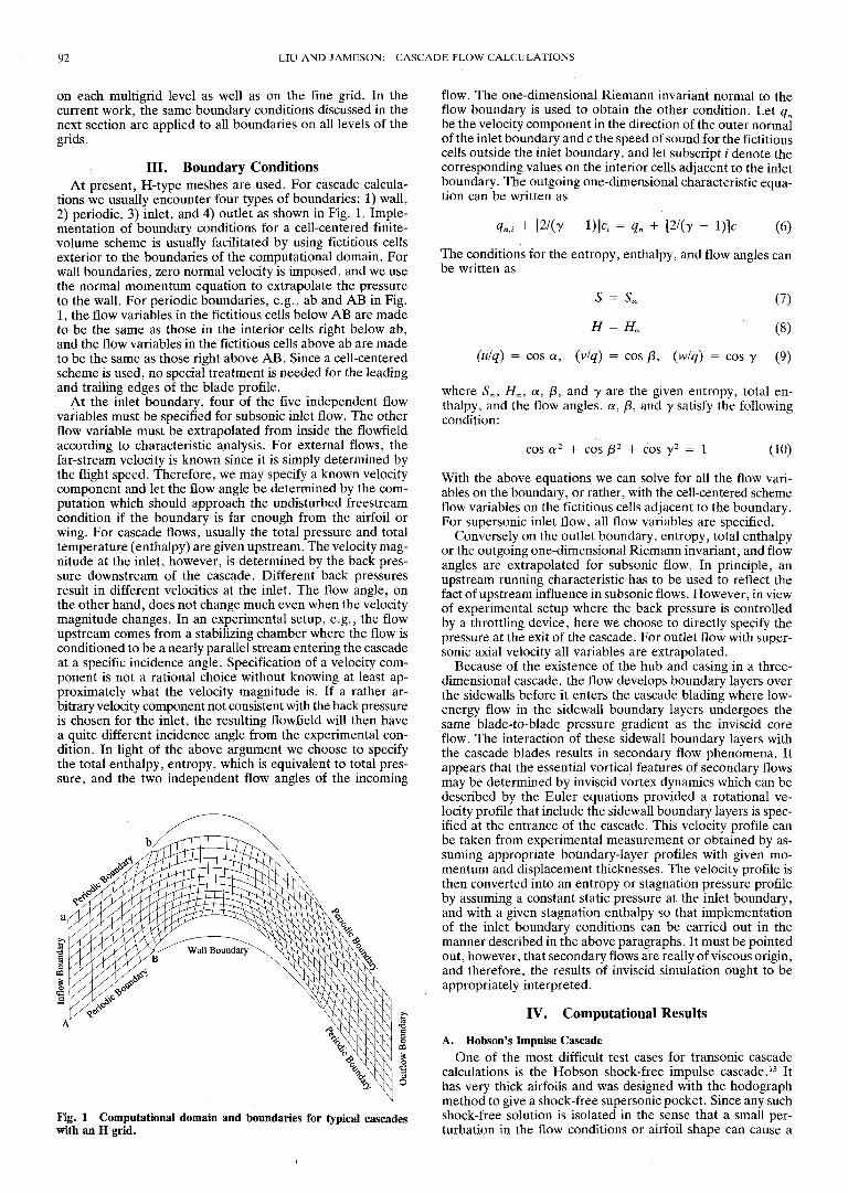
The result, however, showed a noticeable shock terminatingthe supersonic pocket in both the Cp distribution and the Machnumber contour plots. Figure 2 shows the Cp distributionobtained by the present method with an 80 x 24 mesh. Forty-eight points are distributed on the upper and lower surfaceseach. It can be seen that the solution is essentially shock freeand in close agreement with the original hodograph design.Figure 3 shows the Mach number contours of the same so-lution. Because this cascade is shock-free and geometricallysymmetric before and after in the stream wise direction, theflowfield should be symmetric likewise. If for any reason ashock is present in the passage, then the flowfield would nolonger be symmetric. The smooth symmetric pattern shownin Fig. 3 is an indication of the accuracy of the solution.

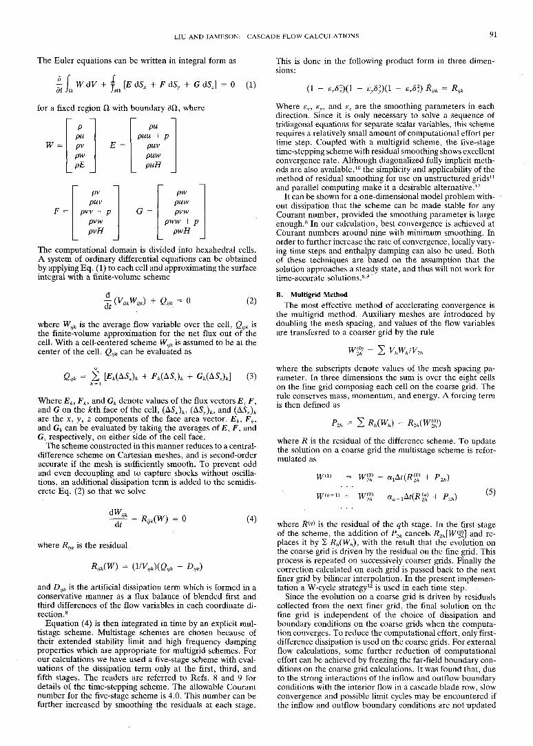
B. Supersonic Wedge CascadeDenton presented a supersonic wedge cascade in Ref. 1 as

a test case for capturing oblique shocks in cascades. Figure 4shows the profile of the cascade and the pressure contours ofa solution with inlet Mach number 2 calculated by the present

I

I

—— Hodograph Design+ Upper surface* Lower surface

80x24 mesh

Fig. 2 Profile and pressure coefficient distribution over Hobson cas-cade.

Fig. 4 Profile and pressure contour of supersonic wedge cascade.

8

.32G °o O

OTto

so

a

* Upper Surface„ Lower Surface

__ Exact

Fig. 3 Mach number contour of Hobson cascade.

Fig. 5 Surface pressure distribution over supersonic wedge cascade.

method. The shock reflected from the lower blade is designedto be exactly cancelled out at the corner of the upper blade,giving a uniform flow between the parallel surfaces and anexpansion off the downstream corner. This design gives a goodtest case for numerical methods, since the inevitable smearingof shock fronts in a shock-capturing method and any possiblewrong prediction of shock angle prevent complete cancella-tion of the reflected shock, and thus produce a nonuniformregion downstream. Figure 5 shows the pressure distributionon the blade obtained by the present method. Comparison ofour results and those by Denton1 shows that the solution ofthe present method has a more uniform flow region after thereflected shock. This is an indication of better resolution ofthe shock waves. However, the reflected shock is still notcompletely cancelled out by the corner of the upper blade.This causes oscillations in both the pressure and Mach numberdistributions as shown in Figs. 5 and 6. In addition, the Machnumber in the expansion region is lower than that of theanalytic solution, although the pressure has fully recoveredto the analytic value as shown in Fig. 5. This is an indicationof entropy production and is caused by the large dissipationincurred at the corner point where the flowfield has a sharpdiscontinuity due to the expansion waves. As pointed out, acomplete cancellation may never be achieved by a shock-capturing method due to the finite thickness of the shockwaves. Improvements, however, may be expected for suchflows by using solution-adaptive grids with more grid pointsclustered near the shocks, or more sophisticated schemes ofhigher shock resolution, such as the TVD or other up winding-type schemes.

C. VKI Turbine CascadeThis is a two-dimensional turbine nozzle cascade.15 Both

the two-dimensional and three-dimensional programs are usedto calculate the flow through this cascade. The three-dimen-sional results with uniform inlet flow are found to be identical


§8I"

Upper SurfaceLower Surface

Exact

Fig. 6 Surface Mach number distribution over supersonic wedgecascade.

Upper surfaceLower surfaceExperiment

76x20x10 mesh

Fig. 7 Isentropic Mach number distribution over VKI cascade at exitisentropic Mach 0.7.

to our two-dimensional solution as they should be. A 77 x21 H-mesh with the same surface definition as proposed inRef. 15 was used in the blade-to-blade plane. The interiorpoints of the mesh are redistributed by an elliptic mesh gen-erator after Thompson et al.16 A three-dimensional mesh isconstructed by stacking these two-dimensional H-meshes inthe spanwise direction, forming a three-dimensional linearcascade with straight side walls. The aspect ratio of the bladeis 0.4. Because of the small aspect ratio, only 11 grid pointsare used in the spanwise direction.

Figure 7 shows the blade surface isentropic Mach numberdistributions of both experiment15 and our calculation for anisentropic exit Mach number 0.7. The comparison shows goodagreement except at the trailing edge of the blade where thenumerical solution shows two points with large suction. Thisis probably due to the fact that we did not use any cusp tomodify the round trailing edge of the blade profile. Figure 8shows the solution of the same cascade at exit isentropic Machnumber 1.0. Good agreement with experimental data is alsoobtained. The fast convergence to be shown below, and the

z"S OOI *.Sn

2 §

CNo

Upper surfaceLower surfaceExperiment

76x20x10 mesh

Fig. 8 Isentropic Mach number distribution over VKI cascade at exitisentropic Mach 1.0.

ResidualMass Difference.Outflow Angle

-79.31°

c

a

o 50 100 150 200 250 300Work Units

76x20x10 mesh, 2 level(s) of multigrid W-Cycle

Fig. 9 Convergence history for VKI cascade at exit isentropic Mach1.0.

good agreement with experimental data without adding a cusp,demonstrate the robustness of the scheme.

Figure 9 plots the convergence history for the transoniccalculation at exit isentropic Mach number 1.0. The compu-tation was done with two levels of multigrids. For three-dimensional calculations, the number of grid points on thecoarse grid is I of that on the fine grid. Measured by a "workunit" consisting of the computational effort of one time stepon the fine grid, the work required for one multigrid cyclewith two levels is 1 + i plus the work required for additionalresidual calculations and data transfer, which is of the orderof 25%. Figure 9 shows that within 200 multigrid time steps,or 225 work units, the residual (shown by the solid line) isdriven to the order of 10 ~10. The dashed line shows the rel-ative difference between the mass flow at the exit and that atthe entrance of the cascade. With this difference driven tothe order of 10 ~10 we can be sure that our calculation properlyconserves mass flow in the cascade passage, which is an im-portant property for internal flow calculations. Such a cal-culation on the 77 x 21 x 11 mesh with 200 multigrid timesteps takes a total of 840 s on a single processor of a Convex


C2 computer in double precision. Double precision was usedonly to show that the scheme is capable of driving the residualbeyond the order of 10 ~7. For engineering applications, theresidual need only be reduced to the order of 10 ~4. Figure 9shows that this can be achieved within a few more than 50time steps. At that time, the mass flow difference and theoutflow angle also show that the solution has effectively reacheda steady state.

Since the Euler equations are capable of describing rota-tional flow, one expects that they can be used to solve flow-fields that involve inviscid vortex transport. In cascade prob-lems, secondary flow is not only important for the performanceof turbomachines, but also interesting, because there has beenthe suggestion that certain features of the secondary flow aredue to the inviscid convection of the vortices developed onthe side walls at the entrance. The Euler equations should beable to predict these features of the secondary flow when giventhe initial boundary-layer type velocity distribution. The or-igin of this velocity distribution is, of course, due to viscosity.However, the later development of the vortex flow and itseffect on the global flowfield, such as the appearance of pas-sage vortices, may be largely an inviscid process. To dem-onstrate this idea, we solved the Euler equations for the VKIcascade with a typical inlet boundary-layer velocity distribu-tion. Twenty-one grid points are used in the spanwise direc-tion for this calculation. They are distributed in such a waythat the grid has a better resolution near the end-walls tocapture the boundary-layer type velocity profile.

Figure 10 shows the swirl in two cross sections of the cascadeflowfield. The swirl is defined to be the dot product of thevorticity and velocity vectors normalized by the magnitude ofthe velocity. Therefore, it is essentially the streamwise vor-ticity and can be used as a good indication of secondary flow.Cross section A-A cuts through the two counter-rotatinghorseshoe vortices generated in front of the leading edge asa consequence of the interaction of the side-wall boundarylayers and the blade. Each of the horseshoe vortices branchinto two legs downstream on either side of the blade. Thebranches on the pressure side, however, have the same senseof rotation as the passage vortices generated by the pressuregradient between the upper and lower blades, and therefore,cannot be distinguished from the larger passage vortices. The

B-B

Negative SwirlPositive Swirl

suction side branch of the horseshoe vortices have the op-posite sense of rotation and can still be seen downstream incross section B-B.

D. Low-Pressure Turbine CascadeThis is a turbine cascade with blade profile typical of the

root section of a low-pressure aircraft gas turbine. Its sidewalls have a 6-deg divergence in the blade passage. The cas-cade has been extensively tested and analyzed by Hodson andDominy.5~7 At its design condition this cascade has an exitisentropic Mach number of 0.7 and an incidence angle of 38.8deg. We calculated this case with a 80 x 16 x 16 mesh.Figure 11 is the typical convergence history for our calcula-tions with three levels of multigrid. Figure 12 shows the is-

s3

ResidualMass Difference.Outflow Angle

0 50 100 150 200 250 300

Work Units80x16x16 mesh, 3 level(s) of multigrid W-Cycle

Fig. 11 Convergence history for a low pressure turbine cascade atdesign condition.

Upper surfaceLower surface

Experiment

80x16x16 mesh

Fig. 12 Midspan isentropic Mach number distribution at design con-Fig. 10 Contours of swirl of VKI cascade in two cross-sectional planes. dition over a low pressure turbine cascade.


entropic Mach number distribution at midspan, together withthe experimental data taken from Ref. 6. It is pointed out inRef. 6 that there is a separation bubble at about 0.8 chordon the upper surface of the blade. This seems to explain theslight discrepancy between the experimental data and ourinviscid solution. The inviscid solution gives a greater adversepressure gradient than the real viscous flow. The viscous flowcannot sustain the large adverse pressure, and thus separates,changing the outer inviscid flow.

Notice that our solution also predicts a suction peak nearthe leading edge. This suction peak is followed by a sharpdiffusion, and therefore, is likely to cause separation too.Although the experimental data do not show this suction peak,Hodson5 observed a small separation bubble near the leadingedge. In fact, at a larger incidence angle this suction peakbecomes obvious in the measured data too. Figure 13 showsthe computed and measured isentropic Mach number distri-bution at an 8.6-deg positive incidence angle relative to thedesign condition. The measured data is taken from Ref. 7.We can see that the leading-edge suction peak on the uppersurface is increased, while that on the lower surface disap-pears. Overall agreement between experiment and compu-tation is still obtained.

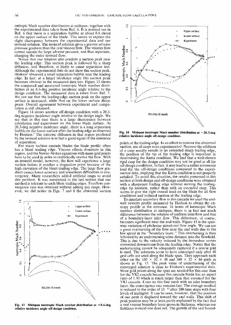
Figure 14 shows another off-design condition with a 20.3-deg negative incidence angle relative to the design angle. Wesee that in this case there is a large discrepancy betweencalculation and experiment on the lower blade surface. At20.3-deg negative incidence angle, there is a long separationbubble on the lower surface after the leading edge as observedby Hodson.7 The extreme diffusion in that region predictedby the inviscid solution is in fact a good signal of the existenceof separation.

For many turbine cascade blades the blade profile oftenhas a blunt trailing edge. Viscous effects dominate in thisregion, and the Navier-Stokes equations with many grid pointshave to be used in order to realistically resolve the flow. Withan inviscid model, however, the flow will experience a largesuction before it reaches a stagnation point because of thehigh curvature of the blunt trailing edge. The large flow gra-dient causes lower accuracy and sometimes difficulties in con-vergence. Many researchers added artificial cusps to avoidthis problem. It was mentioned in the last section that ourmethod is tolerant to such blunt trailing edges. Excellent con-vergence rate was obtained without adding any cusps. How-ever, we did notice in Figs. 7 and 8 the abnormal suction

Upper surfaceLower surface

Experiment

£ < =&

Upper surface

Lower surfaceExperiment

80x16x16 mesh

Fig. 13 Midspan isentropic Mach number distribution at + 8.6-degrelative incidence angle off-design condition.

80x16x16 mesh

Fig. 14 Midspan isentropic Mach number distribution at — 20.3-degrelative incidence angle off-design condition.

points at the trailing edge. In an effort to remove the abnormalsuction, use of cusps were experimented. Because the additionof a cusp usually results in an extended sharp trailing edge,the position of the tip of the trailing edge is important indetermining the Kutta condition. We find that a well-chosenrigid cusp for the design condition may not be good at all foroff-design conditions. In fact, it may lead to a rather erroneousload for the off-design conditions compared to the experi-mental data, implying that the Kutta condition is not properlysatisfied. To avoid this situation, the results presented in thissection at both design and off-design conditions were obtainedwith a sharpened trailing edge without moving the trailing-edge tip location, rather than with an extended cusp. Thisseems to give the right overall load on the blade for all flowconditions and reduced suction at the trailing edge.

To simulate secondary flow in this cascade we used the end-wall velocity profile measured by Hodson to obtain the en-tropy profile at the entrance. In terms of isentropic Machnumber distribution at midspan, there is in fact not muchdifference between the solution of uniform inlet flow and thatof a boundary-layer inlet flow. This difference, of course,becomes significant near the end walls. Figure 15 is the span-wise variation of pitch wise mixed-out flow angle. We can seea great overturning of the flow near the end walls due to thelow speed in the "boundary layer." This overturning is thenfollowed by an underturning some distance into the flowfield.This is due to the velocity induced by the horseshoe vortexconvected downstream from the leading edge. Notice that theunderturning cannot be adequately captured if a coarse gridis used. The solutions seem to have converged only after 48grid cells are used along the blade span. They approach eachother on the 160 x 32 x 48 and 160 x 32 x 64 grids asshown in Fig. 15. The peak value of underturning of theconverged solution is close to Hodson's experimental data.More grid points along the span are needed for this case thanfor the VKI cascade because this cascade blade has an aspectratio of 1.93 which is much larger than that assumed for theVKI cascade. Even on this fine mesh with an inlet boundarylayer, the convergence rate remains fast. The average residualis reduced to the order of 10~ lD after 100 time steps with fourlevels of multigrid. It can be seen, however, that the positionof our peak is displaced toward the end walls. This shift ofpeak position may be at least partly explained by the fact thata real viscous boundary layer grows in thickness, whereas ourfictitious inviscid one does not. The growth of the real bound-


80x16x2480x16x3280x16x4880x16x64Experiment

z/h0.5

Fig. 15 Spanwise distribution of pitchwise-mixed exit flow angle at140% axial chord.

3.0 -T

2.5 -

2.0 -

1.5 -

1.0 -

0.1 0.2 0.3 0.4 0.5

Fig. 16 Secondary velocity vectors and vorticity contours at 140%axial chord.

ary layer will displace the fluid away from the wall, and there-fore, cause the vortex to be pushed further inside.

Figure 16 shows the secondary velocity vector field and thevortex contours at 140% Cx. The secondary velocities wereobtained by projecting the velocity vectors onto the planeperpendicular to the mixed-out flow direction at the section.The vorticity is then calculated on that plane and plotted withplotSd (the flow visualization package from NASA AMES).Comparison with that obtained by Hodson6 from an experi-ment shows that although the positions of the vortices do notagree very well with experiments, the computational resultspredict qualitatively the same vortex structure.

V. Concluding RemarksA multigrid finite-volume method for the Euler equations

has been developed for calculating two- and three-dimen-sional cascade flows, including flows with end-wall boundary-

layer velocity profiles. An explicit multistage time-steppingscheme is used. The stability limit of the explicit scheme isextended by using implicit residual averaging. Convergenceis accelerated by using local time stepping, enthalpy damping,and most of all a multigrid method. The method has beenused to calculate the flow through Hobson's shock-free im-pulse cascade, a supersonic wedge cascade, the VKI turbinenozzle, and a low-pressure turbine cascade with end-wallboundary-layer profiles. Good convergence and overall ac-curacy can be obtained for blades with blunt trailing edgeswithout adding a cusp. Reduction of residuals in the order offour orders of magnitude is achieved generally within 50-100times steps. Comparisons with experiments show good ac-curacy of the method at design conditions. At off-design con-ditions, however, large separation bubbles may exist and aNavier-Stokes solver must be used. Qualitative results supportthe idea that the Euler equations are capable of capturing thesecondary flow vortices which develop as a consequence ofinviscid convection of the entrance velocity profile. Quanti-tative prediction of secondary flows with an Euler method,however, need be cautioned.

AcknowledgmentsThis research was supported by the Office of Naval Re-

search under Grant N00014-89-J-1366, the Defense AdvancedResearch Projects Agency under Grant N00014-86-K-0759,and the International Business Machines Corporation undera grant dated June 15, 1989. The authors are grateful for theirsupport.

References'Denton, J. D., "An Improved Time Marching Method for Tur-

bomachinery Flow Calculation," Journal of Engineering for Gas Tur-bines and Power, Vol. 105, July 1983, pp. 514-521.

2Jameson, A., Schmidt, W., and Turkel, E., "Numerical Solutionof the Euler Equations by Finite Volume Methods Using Runge-Kutta Time Stepping Schemes," AIAA Paper 81-1259, June 1981.

3Holmes, D. G., and Tong, S. S. "A Three-Dimensional EulerSolver for Turbomachinery Blade Rows," Journal of Engineering forGas Turbines and Power, Vol. 107, April 1985, pp. 258-264.

4Smith, W. A., and Caughey, D. A., "Multigrid Solution of In-viscid Transonic Flow Through Rotating Blade Passages," AIAAPaper 87-0608, Jan. 1987.

5Hodson, H. P., and Dominy, R. G., "Boundary Layer Transitionand Separation Observed Near the Leading Edge of a High SpeedTurbine Blade," Journal of Engineering for Gas Turbines and Power,Vol. 107, Jan. 1985, pp. 127-134.

6Hodson, H. P., and Dominy, R. G., "Three-Dimensional Flowin a Low Pressure Turbine Cascade at its Design Condition," Amer-ican Society of Mechanical Engineers Paper 86-GT-106, June 1986.

7Hodson, H. P., and Dominy, R. G., "The Off-Design Perfor-mance of a Low Pressure Turbine Cascade," American Society ofMechanical Engineers Paper 86-GT-188, June 1986.

8Jameson, A., Transonic Flow Calculations, MAE Rept. 1651,Princeton Univ., Princeton, NJ, July 1983.

9Liu, F., "Numerical Calculation of Turbomachinery CascadeFlows," Ph.D. Dissertation, Princeton Univ., Princeton, NJ, June1991.

10Puliiam, T. H., and Steger, J. L., "Recent Improvements inEfficiency, Accuracy and Convergence for Implicit Approximate Fac-torization Algorithms," AIAA Paper 85-0360, Jan. 1985.

HMavriplis, D. J., and Jameson, A., "Multigrid Solution of the2D Euler Equations on Unstructured Triangular Meshes," AIAAPaper 87-0353, Jan. 1987.

12Jameson, A., "Successes and Challenges in Computational Aero-dynamics," AIAA Paper 87-1184, June 1987.

13Hobson, D. E., "Shock-Free Transonic Flow in TurbomachineryCascades," Univ. of Cambridge, Dept. of Engineering Rept. CUED/A Turbo/TR 65, Cambridge, England, UK, 1974.

14Ives, D. C., and Liutermoza, J. F., "Second-Order-AccurateCalculation of Transonic Flow over Turbomachinery Cascades," AIAAJournal, Vol. 17, No. 8, 1979, p. 870-876.

15Sieverding, C., "Test Case 1: 2-D Transonic Turbine NozzleBlade," Numerical Methods for Flows in Turbomachinery Blading,von Karman Inst. for Fluid Dynamics Lecture Series 1982-05, RhodeSaint Genese, Belgium, April 26-30, 1982.

16Thompson, J. F., Thames, F. C., andMastin, C. W., "AutomaticNumerical Generation of Body-Fitted Curvilinear Coordinate Sys-tems for Fields Containing Any Number of Arbitrary Two-Dimen-sional Bodies," Journal of Computational Physics, Vol. 15, July 1974,pp. 299-319.

cascade flow calculations by a multigrid euler method flow calculations by a multigrid euler method...

Documents