capital structure in european smes - pure
TRANSCRIPT

MSc. Finance & International Business Authors:
Niels Stoustrup Jensen (270404)
Fabian Thomas Uhl (280905)
Academic advisor:
Jan Bartholdy, PhD
Capital Structure in European SMEs
An analysis of firm- and country specific variables
in determining leverage
Aarhus School of Business
University of Aarhus
Aug. 2008

ABSTRACT
This study investigates how country specific factors related to macroeconomic development,
corporate governance, legal- and financial environment affect the capital structure of
European small and medium sized enterprises. Using regression analysis on a data panel
consisting of nearly 500,000 observations from a total of 24 countries, the study shows
significant relationships between proxies for different institutional factors and leverage. This
suggests that policy makers can affect the environment for SMEs to operate in, by improving
certain country characteristics. By distinguishing between Eastern and Western Europe using
a dummy variable, the study further shows that there are differences in the impact of firm as
well as country specific variables on leverage, depending on the region a company is
incorporated in.
More specifically, the study finds evidence that leverage is in general lower in Eastern
Europe. This does to some extend support the findings of the OECD, that there exist an SME
financing gap in transition countries which is argued to be due to a lack of institutional
development, affecting the credit availability of SMEs.
The expectation that corporate governance, legal- and financial environment are positively
related to leverage, is only partly supported since a few surprising results are obtained
regarding certain variables. Contrary, there is clear evidence that bank concentration is
negatively correlated to leverage. Further, more profitable banks enhance the level of debt in
the capital structure of SMEs.
The study thereby questions the ability of the traditional ground pillars of capital structure
theory, namely the static trade-off- and pecking order theory, to fully explain leverage, since
they are argued to not sufficiently take into account the supply side of the financing decision.
Obligatory note to the reader
We hereby declare that this paper has been produced in full cooperation by the two authors.
No division has been done in terms of workload, and each of us is therefore responsible for
the entire paper.
Best regards,
Fabian Thomas Uhl
Niels Stoustrup Jensen

Table of Contents
1. Introduction ............................................................................................................ 1
1.1. Outline of the paper ............................................................................................ 2
2. Literature review .................................................................................................... 3
2.1. Theories of capital structure ............................................................................... 3
2.2. Miller and Modigliani’s irrelevance proposition ................................................ 3
2.3. The static Trade-off theory ................................................................................. 5
2.4. Pecking order theory ......................................................................................... 11
2.5. SME financing gap ........................................................................................... 15
2.6. Capital structure in East vs. West ..................................................................... 17
2.7. Market power .................................................................................................... 21
3. Research question and hypotheses ..................................................................... 24
4. Methodology ......................................................................................................... 27
4.1. Fixed effects vs. random effects model ............................................................ 27
4.2. Dummy variables .............................................................................................. 30
5. Data collection ...................................................................................................... 34
5.1. Firm specific data .............................................................................................. 34
5.2. Country specific data ........................................................................................ 37
5.3. The final dataset ................................................................................................ 38
6. Proxies ................................................................................................................... 39
6.1. Dependent variables .......................................................................................... 39
6.2. Independent variables ....................................................................................... 41

7. Analysis ................................................................................................................. 54
7.1. Descriptive statistics ......................................................................................... 54
7.2. Regression output ............................................................................................. 61
8. Interpretation of results ....................................................................................... 64
8.1. Hypothesis 1 – Leverage in Eastern and Western Europe ................................ 64
8.2. Hypothesis 2 – Corporate governance .............................................................. 65
8.3. Hypothesis 3 – Legal environment ................................................................... 67
8.4. Hypothesis 4 – Financial development ............................................................. 72
8.5. Hypothesis 5 – Bank concentration .................................................................. 75
8.6. Hypothesis 6 – Bank profitability ..................................................................... 76
8.7. Hypothesis 7 – Eastern and Western Europe respond differently .................... 78
9. Conclusion ............................................................................................................. 90
10. Critical assessment and suggestions for further research ................................ 93
11. Bibliography ......................................................................................................... 96
12. Appendices – Table of contents ......................................................................... 104

MSc Finance & International Business
1
1. Introduction
Ever since Miller and Modigliani in 1958 stated their famous irrelevance proposition,
capital structure theory has been of great interest to many scholars around the world.
Out of the wide body of research that has evolved over the last fifty years, the static
trade-off and pecking order theories are standing as the ground pillars of capital
structure theory. Lots of empirical work has so far been conducted in order to test the
two theories, and some has tried to favor one over the other. But today, there is still no
clear cut answer to what theory fits reality the best. Instead it seems like both theories
has its drawbacks and are only partly able to explain capital structure of companies.
The vast majority of the empirical work on capital structure has in the past been carried
out on large listed companies in the US due to data availability. This research paper will
instead focus on the capital structure of small and medium sized enterprises (SMEs) in
Europe. According to the OECD, SMEs in OECD countries stand for 60-70 percent of
net job creation and contribute innovation and general dynamism to the economy. This
gives an idea of the immense importance of SMEs in all economies. Acknowledging
this fact, policy makers around the world should be concerned about fostering a fruitful
environment for SMEs in order to promote growth. Different scholars have concluded
that institutional factors are able to explain parts of the deviation in capital structure in
cross country studies. This has lead to the primary motivation behind this research
paper, which is to identify some of these country specific factors, and to determine their
impact on capital structure. This rests on a belief that some SMEs, especially in
transition countries, find it hard to acquire appropriate external financing in order to
pursue their growth opportunities. This is supported by the OECD, who is specifically
talking about an “SME Financing GAP”, which is determined by a country’s
macroeconomic, legal, regulatory and financial development (OECD 2006).
This study is based on an analysis of the capital structure of companies from 24 Eastern
and Western European countries. The goal of the analysis is to identify significant
relations between firm specific as well as country specific factors, and leverage. The
study then goes one step further by testing whether there are differences between
Eastern and Western Europe in the use of leverage, and more importantly, whether the
impact of different variables on leverage is different between the two samples. This can
generally be summed up to the following central research question:

MSc Finance & International Business
2
Central research question:
“To what extend do country specific variables concerning macroeconomic
development, corporate governance, legal and financial environment help in explaining
leverage in small and medium sized enterprises in Eastern and Western Europe”
Besides, hopefully contributing valuable information to policy makers on which factors
affect SMEs access to finance, it can potentially add explanatory power in terms of
better predicting the capital structure of companies. It is suggested that the traditional
capital structure theories do not, to a sufficient extend, take into account country
specific factors that influence SMEs access to external financing, and therefore only
present an incomplete picture. Specifically, the supply side of external finance is not
sufficiently reflected in the traditional theories of capital structure. The authors of this
study suggest that especially for SMEs, that usually do not have access to international
capital markets, the potential lack in supply of external finance is an important
determinant of capital structure that cannot be ignored.
1.1. Outline of the paper
The paper will continue as follows. Section 2 will consist of a literature review going
over the two main theories of capital structure along with relevant empirical evidence.
The literature review will also cover previous work on differences in capital structure
between Eastern and Western Europe, along with a discussion of what institutional
factors can potentially be responsible for this. Section 3 will state the research question
and formulate the hypotheses that are going to be investigated in the paper. Section 4
will carry forward by describing the adopted methodology to test the hypotheses.
Section 5 will describe the data collection including the different data sources and
discuss the processing of the data in terms of eliminating outliers, observations with
missing data etc. The adopted methodology implies the use of different proxies, which
will be presented and discussed in section 6, together with expectations regarding their
individual impact on leverage. Section 7 will present the results from the statistical
analysis while these will be interpreted in section 8. The final conclusion of the paper
will be presented in section 9.

MSc Finance & International Business
3
2. Literature review
2.1. Theories of capital structure
Trying to understand how firms choose their capital structure has been of great interest
to scholars around the world for a very long time. Most effort has been done trying to
explain the proportion of debt relative to equity, instead of the exact combination of
different kinds of securities, such as long-term vs. short-term debt etc. During the last
50 years, several different theories have emerged. The next section will give a short
review of Miller and Modigliani’s theory of the irrelevance of the financing decision
which started the era on capital structure research. After that, a review of today’s most
popular theories on capital structure, namely the trade-off and pecking order theories
will be performed. According to (Frank, Goyal 2007), both of these theories are so
called “point of view” –theories. A “point of view” –theory is characterized by offering
a framework or guidelines, in which explicit models can be developed. It formulates
some basic underlying principles and ideas that should serve as guidelines, whereas e.g.
the well known Capital Asset Pricing Model (CAPM) is explicitly expressed in
mathematical terms. Therefore when testing the pecking order or trade-off theory, it is
necessary to formulate a specific model, which requires different assumptions to be
made (Frank, Goyal 2007).
2.2. Miller and Modigliani’s irrelevance proposition
The extensive number of research papers within the field of capital structure accelerated
after 1958, where the later Nobel Prize awarded, Merton Miller and his colleague
Franco Modigliani published their seminal paper on capital structure (Modigliani,
Merton H. Miller 1958). In this paper they presented what is nowadays often referred to
as M&M’s proposition I, also known as “The Irrelevance Proposition”, which is
considered to be the first real theory on capital structure, even though a similar idea was
presented by (Williams 1938) 20 years before. As a matter of fact, (Weston 1955)
argued that several teachers of business finance at that time actually doubted whether it
was possible at all to develop theories of capital structure. Therefore it most likely came
as a surprise when M&M in their paper stated that financing is irrelevant. Explicitly
M&M stated the following (Modigliani, Merton H. Miller 1958, p. 268):

MSc Finance & International Business
4
“The market value of any firm is independent of its capital structure and is given by
capitalizing its expected return at the rate ρk appropriate to its class.”
Mathematically, this is expressed by the simple equation below, similar to saying that
the value of a levered firm is equal to the value of an unlevered firm.
VL = VU
The underlying logic behind M&M’s proposition was that the value of a pizza does not
depend on how it is sliced (Myers 2001). Applying this intuitive point of view to a
company basically means that depending on the composition of assets on the left hand
side of the balance sheet, a company will receive a given expected stream of cash flows.
Finding the value of the company is then done by capitalizing these cash flows at the
appropriate discount rate, depending on the operating risk of the company. According to
the irrelevance theory, the amount of debt relative to equity only serves to determine the
successive split of cash flows between debt holders and equity holders, and does not
affect the aggregate value of the company. M&M proved that under their assumptions,
investors can create “home-made leverage”, by borrowing at the risk-free rate and
buying stocks in an unlevered company. The other way around, shareholders can also
undo unwanted leverage in a company by buying fewer stocks and lend money at the
risk-free rate. Because investors can easily create or undo leverage on there own, the
rationale is that they should not be willing to pay a premium for companies with a
specific capital structure, due to possible arbitrage. Hence the value of two differently
levered, but otherwise identical companies should be equal.
However, no matter how appealing this simple statement sounds, it only holds in the
synthetic world of M&M, where capital markets are perfect, i.e. no taxes, no business
disruption costs etc. But even though the theory today does not make much sense
because of the many strict and unrealistic assumptions, it brought about something else
very valuable, namely focus on capital structure theory. “The Irrelevance Proposition”
triggered a wave of research trying to develop evidence against M&M, i.e. that
financing actually matters. Referring to the pizza again, (Myers 2001) argues that the
value of a pizza actually depends on how it is sliced, since consumers gladly pay more
for the many slices, than for a whole pizza.

MSc Finance & International Business
5
2.3. The static Trade-off theory
Probably due to the many critics of the unrealistic assumptions behind their proposition
1, M&M added taxes to their, still hypothetical world, in a later paper (Modigliani,
Merton H. Miller 1963). By taking into account that interests were (and in most
countries to some extend still are) tax deductable and therefore decreased the amount of
taxes to be paid, their model introduced an interest tax shield. When debt is assumed to
be risk-free, and there is no “counterweight” in the form of increasing costs due to high
leverage, this resulted in an optimum capital structure consisting of 100% debt. This
theoretical optimum fits very badly with the empirical observations, and that was
probably one of the things that helped the trade-off theory to quickly become so
popular. The trade-off theory suggests namely that the optimal capital structure is based
on a trade-off between the value of the interest tax shield and the costs associated with
leverage. The optimal capital structure is at the point where the marginal increase in the
costs associated with additional leverage exactly offsets the marginal benefit of the
increase in the interest tax shield from additional leverage. Traditionally when referring
to “the costs associated with leverage”, one explicitly meant direct costs of bankruptcy
i.e. lawyers fees, administration expenses etc. However a study (Warner 1977) showed
that the direct costs of bankruptcy are negligible, and therefore do not alone rationalize
the observed moderate borrowing among most firms. In a study among others (Altman
1984), evidence was found, indicating that indirect costs are way more important than
direct costs, which is one of the reasons why we today refer to the costs associated with
high leverage as business disruption or financial distress costs. Examples of indirect
costs of bankruptcy that are incurred because of being highly levered, could be lost
business or lost investment opportunities (Copeland 2005). Below a graphical
presentation of the trade-off theory is shown. It can be seen that after some point (the
optimum), the marginal financial distress costs are bigger than the marginal benefits
from the interest tax shield, resulting in a decrease in the market value of the company.

MSc Finance & International Business
6
Figure 1
Source: (Myers 1984)
2.3.1. Agency costs and the trade-off theory
(Myers 2001) argues that agency costs are also a part of financial distress costs, and an
important contribution to the trade-off theory because it adds further counterweight to
the interest tax shield, helping to justify the moderate borrowing that is usually observed
in empirical findings. (Jensen, Meckling 1976) is probably one of the most well known
articles describing different principle-agent conflicts and the agency costs in connection
with these. Specifically relevant to the trade-off theory, the paper describes the agency
costs associated with debt.
One of the things described, is what the authors call “The Incentive Effects Associated
with Debt”. This concerns the fact that there is an asymmetric payoff scheme between
debt and equity holders. Equity holders have a residual claim on the company, whereas
debt holders (if we assume non-convertible debt and other forms of equity-like
securities) have a fixed promised payoff. If the manager acts 100% in the interest of
shareholders, he would have an incentive to transfer wealth from debt holders to equity
holders. This is possible through “risk shifting”, where after receiving debt financing
conditional on a certain project, the company undertakes a different project with higher
volatility. Even though the expected value of the project as a whole might be the same,
equity holders will increase their expected payoff because they have an upside chance,
while debt holders will see the value of their claim diminishing. The explanation for this

MSc Finance & International Business
7
is that debt holders in a “good scenario” still only get their promised pay off due to the
way a usual debt contract is constructed, while equity holders get the rest of the value.
In a “bad scenario” where the company becomes worthless, debt holders get nothing
exactly as equity holders. The incentive behind risk shifting can be illustrated very easy
by considering the two scenarios as the only possible outcomes. Since equity holders
never get anything in the bad scenario but get more in the good scenario depending on
volatility, there is an incentive to increase the risk, in order to get the highest expected
value from their perspective. For a numerical example of risk shifting see Appendix 1.
Debt holders are of cause aware of this incentive, and will therefore demand debt
covenants or monitoring devices in order to avoid such behavior of the stockholders
who have the ultimate control over the company. Since the costs associated with debt
covenants and especially monitoring devices are material, it will directly result in more
expensive borrowing in order to compensate for the additional costs. Therefore the
potential incentive among some borrowers to cheat the lenders, will effectively mean
that all borrowers (with good or bad intentions), will end up paying more for their loans
than if such an agency conflict did not exist between the two groups of capital
providers. Another consequence of debt covenants could be that managers are constraint
in their ability to distribute company profits to the stockholders, because the covenant
could restrict doing so if not certain economic key ratios are reached. Furthermore it
could be specified that additional borrowing is only possible under certain conditions or
that further borrowing is even prohibited. If covenants are violated, it could result in the
entire loan to fall due, and therefore the threat of financial distress could mean that the
company has to pass up profitable investment opportunities. This is not a direct
financial cost, but certainly a serious cost in terms of lost flexibility in that managers are
restricted to take certain actions because of the covenants. To sum up, agency costs
makes the use of debt less attractive because of financial as well as non-financial costs
associated with it.
2.3.2. Dynamic trade-off theory
One major drawback of the static trade-off model is that it is a “static” one-period
model. The model solves for the best possible capital structure given the factors
discussed above (interest tax shield, distress costs etc.) and implicitly assumes that all
companies should at all time be at the optimal capital structure (Frank, Goyal 2007).
However it is not realistic to expect companies to plan the financial structure only one

MSc Finance & International Business
8
period ahead. This fact resulted in several scholars turning away from the underlying
ideas of the trade-off theory (taxation and bankruptcy costs) and instead focusing on
other theories trying to explain capital structure (Frank, Goyal 2007). In the later years,
interest for a model based on the traditional trade-off ideas, but incorporating the fact
that capital structure planning is not a 1 period problem, has increased leading to the
formulation of a “dynamic trade-off theory”. By emphasizing for instance transaction
costs, several dynamic models have emerged in the literature, leading to somewhat
different conclusions. The underlying idea of all dynamic trade-off models is however
that the optimal capital structure in period t+1 depends on the optimal capital structure
in period t+2 which depend on t+3 and so on.
One interesting thing about dynamic trade-off models is that they essentially allow
companies to be at suboptimal levels of leverage. By introducing transactions costs it is
not efficient to make constant rebalancing of the capital structure, which will from time
to time drive companies away from their optimal capital structure. (Fischer, Heinkel &
Zechner 1989, p. 19) finds that: “even small recapitalizing costs leads to wide swings in
a firm’s debt ratio over time”. The authors thereby state that recapitalizing costs or
transaction costs are responsible for the observed deviations in capital structure for
companies that are essential similar. At the same time they argue that all else equal,
similar companies should have the exact same recapitalizing criteria’s. Interestingly
they find that smaller companies display larger swings in their capital structure which
could be interpreted as a sign of higher transaction costs for SMEs.
2.3.3. Empirical findings concerning the trade-off theory
A major weakness of the trade-off model is that it is very difficult to test. Nevertheless,
several studies have tried to test the theory in different ways, and some of them will be
highlighted in the following. One study (MacKie-Mason 1990) finds evidence that the
amount of tax loss carry-forwards is negatively correlated to the amount of new debt
issues. This is in line with the trade-off theory, since large tax loss carry-forwards
would make the interest tax shield created through the use of debt redundant if the
company does not earn enough taxable income to benefit from both.
(Bradley, Jarrell & Kim 1984) also interprets their study as supporting a theory of
optimal capital structure i.e. trade-off theory. The support is based on results showing
that volatility of earnings has an impact on leverage together with strong industry

MSc Finance & International Business
9
effects. The intuition according to the trade of theory is that when considering a given
level of costs associated with actual bankruptcy proceedings, the volatility of earnings
has an impact on the expected bankruptcy costs by simply affecting the probability of
default. Therefore companies in risky businesses where earnings are highly volatile will
incur higher levels of expected bankruptcy costs, and should therefore lever to a smaller
degree. The strong industry effects are interpreted as being in favor of an optimal capital
structure which is the trademark of the static trade-off theory. This is because factors
like the magnitude of financial distress costs, non-debt tax shield and the variability of
firm value, are expected to exhibit similarities within different industry classes. This
expectation does not seem very far fetched, since obvious determinants of bankruptcy
costs like e.g. the amount of tangible assets is highly industry specific.
Other studies have used a “target adjustment model” for testing whether companies over
time adjust towards an optimal capital structure. See for example (Auerbach 1985) or
(Jalilvand, Harris 1984). They find significant adjustment coefficients, and interpret it
as support for target adjustment behavior, hence also as support for the trade-off theory.
But before one gets too excited about these findings it should be noted that the statistical
power when testing the target adjustment model is essentially non-existing according to
(Shyam-Sunder, Myers 1999). In their paper, Shyam-Sunder and Myers test the
statistical power of the target adjustment model by applying it to a hypothetical dataset
generated by following the pecking order model. Interestingly they find the target
adjustment model to be accepted even though the observations in the simulated dataset
were created, strictly based on pecking order behavior. They also did the experiment the
other way around, by testing the pecking order theory based on a dataset generated
based on an alternative capital structure theory, and here the pecking order hypothesis
was correctly rejected. According to this evidence, one should be careful when
interpreting tests of the trade-off theory. (Myers 2001, p. 94) explains it in the following
way: “such results might support the theory if it were the only game in town…”. The
point here is that several ideas about capital structure exist, so one cannot test whether
one is correct over the others if you are not aware of the expectations about the other
theories. Otherwise one implicitly applies the logic of Erasmus Montanus1 when he tells
his mother that because a stone does not fly, and she does not fly, she must be a stone.
1 Erasmus Montanus is the name of a play written by Ludvig Holberg in 1723

MSc Finance & International Business
10
Naturally there are also studies that fail to find support of the trade-off theory or where
there is only partly evidence in favor of it because some puzzling results show up at the
same time. And finally some argues that there is no reason to believe that the static
trade-off theory has any explanatory power in terms of the amount of leverage that
companies take on. Critics point out that it is very hard for the trade-off theory to
explain why quite some profitable firms for years have been running at only moderate
levels of debt (Myers 2001). (Graham 2000) concludes that the average company in a
subsample consisting of half the companies in his survey could add a non-trivial
amount, equal to approximately 7.5 % to its value by increasing leverage. In the end,
one must conclude that the opinions about the validity of the trade-off theory are split.
2.3.4. SMEs and the trade-off theory
Traditionally, most research on capital structure including the trade-off theory has been
performed on samples consisting of large listed US firms, due to the better availability
of data. The scope of this paper is concerned with SMEs and therefore it is felt
necessary to elaborate on whether one can expect SMEs to behave similar to large listed
companies in terms of the trade-off theory. Some scholars argue that the actions taken
by managers of SMEs regarding financial decisions can be explained by the same
theories that are usually applied to large listed companies i.e. trade-off and pecking
order (Sogorb-Mira 2005). In the framework of the trade-off theory it is hard to argue
that SMEs would not face the same trade-off between interest tax shield and distress
costs. However it is possible that SMEs might put more emphasis on certain issues or
face problems that large listed companies do not face to the same degree. Here some of
these issues and the possible implications for the capital structure of SMEs will briefly
be discussed.
One possible reason that could explain why SMEs might not follow the trade-off theory
is simple lack of knowledge among managers. If the financing decision should be made
according to the trade-off theory, it is naturally a necessity that managers are aware of
the advantages of an interest tax shield. Within the SME segment, one could expect that
many companies are led by entrepreneurs with their expert skills lying within a field
different from finance, and therefore might not possess the knowledge or for some other
reason, be ignorant of the interest tax shield and therefore do not take advantage of it
(OECD 2006). If managers are not aware of the benefits of leverage, they might tend to
operate at lower debt levels all else equal.

MSc Finance & International Business
11
Another interesting factor is the potential financial constraint of SMEs. If some SMEs
are in fact financially constrained it would mean that independently of whether
managers are aware of the trade-off theory and recognize the advantage of debt, they
might not be able to lever up to their optimal capital structure. This is by the authors
suggested to be an important issue, since that would imply that it is for external reasons
that SMEs might not have sufficient debt according to the trade-off theory. From an
isolated perspective, it does not seem like a big issue if companies have less debt
compared to what is suggested by the theory. But one can imagine serious consequences
if the lack of debt financing results in the company having to pass up profitable
investment opportunities and thereby restricting growth. Lack of debt-financing does
not necessarily mean that no financing is available at all. It can also mean that the price
of the available finance is prohibitive. Section 2.5 will elaborate on this issue.
Finally, one reason why SMEs could have a different capital structure than their large
listed counterparts could be that their “experienced” bankruptcy costs are higher due to
a lot of them being family owned. Besides the expected financial distress costs and the
economic loss due to bankruptcy, a family owned company most likely also represents a
great amount of sentimental value to the owners. Therefore one can argue that this
dimension of distress costs will increase the expected costs of debt, and therefore lower
the optimal capital structure of family owned companies. A convenient thing about this
is that it explains within the framework of the trade-off theory, why the capital structure
of SMEs might deviate from the one of large listed companies.
2.4. Pecking order theory
In 1984, Myers proposed an alternative approach to capital structure theory by
introducing the pecking order theory. This theory states that firms prefer internal
financing to external financing, and if external financing has to be used, the cheapest
possible security is chosen first. Corporations will, when using external finance, first
use debt, then hybrid instruments, and as a last resort, issue equity. In this framework
there is no optimal debt ratio and companies do not try to maintain a target debt-ratio.
Instead, the debt-equity mix of a company is determined by their need for external
finance (Myers 1984).
The basic assumption underlying the pecking order theory is that managers act in the
interest of existing shareholders, and do have better information about the future

MSc Finance & International Business
12
prospects of the company than potential outside investors. A planned stock-issue is
perceived as a bad signal by prospective investors, because they assume that the goal of
the management is to maximize the value of the existing shareholders. The rational
supposition of outside investors is that a company issues shares because management
thinks that the shares of the company are overvalued. Hence, this perceived information
only makes an equity issue possible at a marked-down price. Therefore managers who
are in need of external funds to finance a positive NPV-project, assuming issuance of
debt is not possible, will only consider issuing undervalued shares, if the NPV of the
project is higher than the cost incurred through the undervaluation in the stock-issue.
This means that even when a company has significant growth opportunities, it will not
realize these growth opportunities by means of a stock issue, if the undervaluation due
to the signaling effect, exceeds the potential gains from the projects. Several studies
have confirmed the signaling effect, in that the announcement of a stock issue has a
subsequent negative impact on the stock-price. In a study of large listed companies by
(Asquith, Mullins 1986), the announcement of a stock issue caused an average fall in
the stock-price of about three percent. Furthermore it has been shown that the
magnitude of the price drop is related to how strong the information asymmetry
between inside management and outside investors is. Even if a company has good
prospects for the future, the perceived signaling effect has a negative impact on the
value of the firm in the short-run, i.e. the bad news of a stock issue outweigh the news
of good investment opportunities of the company.
When comparing debt to equity, debt has a senior claim on assets and earnings of the
company. This implies that creditors face less risk compared to equity holders. Only if
the risk of bankruptcy is high, the impact of the announcement of a debt issue will affect
the share-price. Taking this into consideration it can be assumed that only pessimistic
managers will make an equity issue if debt is available at a fair price. The key
predictions of the pecking order theory are therefore as follows:
1) Internal financing is preferred to external financing if available, since
asymmetric information is only relevant for external financing

MSc Finance & International Business
13
2) Changes in the net cash-flow of a listed company will usually be accompanied
by changes in external financing since dividends are in general rather “sticky”,
and cannot be changed in the short-run to finance capital expenditures
3) If external financing is necessary, i.e. the internally generated cash-flow is not
sufficient to cover capital expenditures, debt, which is the safest security, will be
issued first followed by hybrid instruments and then equity.
4) The need for external financing of a company is reflected in its debt ratio
The pecking order theory is therefore, contrary to the trade-off theory, able to explain
why profitable firms have less debt compared to less profitable companies. The reason
is not that they have a low target debt ratio, but that they to a higher degree are able to
generate sufficient internal funds to finance necessary investments (Myers 2001).
2.4.1. Empirical findings concerning the pecking order theory
Like the trade-off theory, contradicting evidence is also observed when turning to the
empirical literature concerning the pecking order theory. However it seems like the
majority of research papers are not able to find convincing overall support of the theory.
A paper that does find evidence for a pecking order is (Shyam-Sunder, Myers 1999). In
the paper, both the static trade-off model as well as the pecking order model is tested.
The paper finds that the pecking order model has more explanatory power than the
trade-off theory, and is a much better first-cut explanation of debt-equity choice. Partly
evidence in favor of the pecking order is found by (Frank, Goyal 2003). These authors
show that large firms show some aspects of pecking order behavior, but do not consider
the results robust enough. A common interpretation in favor of pecking order behavior
is when researchers find a negative correlation between profits and debt. This is also the
argument in (Fama, French 2002), (Titman, Wessels 1988), (Rajan, Zingales 1995) and
others, who find that more profitable firms have less debt.
In a later paper, Eugene Fama and Kenneth French however look critical at the pecking
order (Fama, French 2005). In this article the authors study when, and how often, firms
issue equity. They find that more than half of the companies in their sample violate the
pecking order predictions. This is interpreted from their results showing that between
54% and 72% of their sample depending on the period, makes net equity issues each

MSc Finance & International Business
14
year. Far from all of these companies are under distress, so the pecking order is not able
to explain the behavior of these firms.
(Galpin 2004) argues that the fundamental assumption of the pecking order, that equity
is used as a last resort due to the high issue costs, is not valid. In his study he concludes
that the costs of debt issues often exceed the cost of issuing equity. Galpin shows that
issuance costs have evolved over time. In 1973 debt costs amounted to 50% of equity
costs, increasing to 140% in 2002. This might suggest that the pecking order was valid
at the time it was invented, but that times have changed and it might not hold anymore.
It has to be said that the study was performed on large listed companies and that the
cost-structure could very well be different for SMEs.
2.4.2. SMEs and the pecking order theory
The development of the pecking order theory is largely based on observations from
large listed companies in the US. The structure of SMEs as well as their access to
capital markets is very different to that of large listed companies. Therefore it is
interesting to see if it is possible to verify the validity of the theory for this kind of
companies, similar to what was done regarding the static trade-off theory. Furthermore,
when testing the static trade-off theory or the pecking order theory for SMEs, it is
important to question the reason why SMEs behave according to one theory or another,
since the reason can be very different compared to large listed companies. It turns out
that there are very compelling reasons why the pecking order theory should be able to
explain the behavior of SMEs regarding capital structure. One reason is that small firms
are often owned by only one shareholder who is at the same time the director of the
company. An issue of new equity would dilute the shareholding of the owner-manager,
and can therefore lead to a loss of control in the company. To avoid this, the natural
response would be to turn to debt instead of equity for financing (Lopez-Gracia,
Sogorb-Mira 2008).
Another argument against the use of equity by SMEs is that the cost of external equity
is even higher to them compared to large listed companies. An initial public offering is
not only expensive to organize, but also subject to under pricing which has been shown
to be particularly severe for small companies (Chittenden, Hall & Hutchinson 1996).
Another source of equity finance stems from private placements with private equity
companies or business angels. Apart from the potential loss of control in the company,

MSc Finance & International Business
15
this source of finance also has significant transaction costs due to the complexity of the
contracts that have to be negotiated (Ou, Haynes 2006).
The size of a company also has an impact on the availability of debt-financing. This is
reflected in the fact that smaller companies rely more strongly on short-term financing
than larger companies, since financial constraints are mainly present when attempting to
acquire long-term finance. Therefore the pecking order for SMEs is expanded in the
sense that there is a propensity towards short-term financing over long-term financing
(Lopez-Gracia, Sogorb-Mira 2008). The circumstance that SMEs may be confronted
with constraints in acquiring debt-financing will be discussed in greater detail in the
next section, since it can have a potentially large effect on the capital-structure of SMEs.
2.5. SME financing gap
An issue that has a possible impact on the capital-structure of SMEs is the so-called
“SME Financing Gap”. In a survey performed by the “OECD SME Task Force”, most
OECD member countries agreed that a lack of appropriate financing does have a
negative impact on the growth of innovative SMEs. The “SME Financing Gap” is
commonly defined as the situation where a significant share of SMEs cannot fulfill the
financing needs which exceed their internal financing capacities, through banks, capital
markets or other suppliers of finance. There are different reasons why the financial
constraint of SMEs is larger than that of large companies. One reason is that the
problem of asymmetric information is more severe in SMEs (OECD 2006). This is
partly due to the fact that in many cases the company is very much tied to the
entrepreneur. This leads to a situation where the entrepreneur has considerably superior
information on the situation of the company. Related to this is also the problem that a
manager in an SME is more likely to have insufficient management skills compared to
the managers in large companies. Therefore potential investors have a more difficult
time to assess whether an SME manager is making bad management decisions which
could potentially threaten the well-being of the company. Morale hazard considerations
also play a significant role for the availability of credit to SMEs. The lending bank is
mainly interested in a firm’s capability to repay its loan, while the company might
prefer a high risk and high return strategy, which could lead to risk shifting (see section
2.3.1). Even though risk shifting is a potential problem with any kind of debt financing,
it is usually more severe when lending to SMEs because, as mentioned, the asymmetric

MSc Finance & International Business
16
information present when dealing with SMEs is higher compared to large listed firms
(OECD 2006).
The empirical evidence whether an “SME Financing Gap” exists in reality is rather
mixed depending on region. Most empirical studies have problems with data
availability. Nevertheless there is a general tendency in the empirical studies performed
by the OECD. It has been shown that the financing gap is more severe in OECD
countries that are considered transition countries compared to developed OECD
countries, while it is most significant in non-OECD countries. The research regarding
SME financing has shown that there are different types of financing gaps. For instance
in some emerging countries, the financial system is very much geared towards large
firms, making it much more difficult for SMEs to obtain bank-credit. This leads to a
situation where the growth potential of SMEs is constrained, and the ability of SMEs to
be the innovators of the economy, which is a role they often play, is thereby limited.
Another issue which is particularly widespread in the bank-dominated countries in
central Europe is the rather decent access to debt-financing but a lack of equity-
financing.
It is argued that a crucial component for SME financing is a solid legal, institutional and
regulatory environment. In the case of debt-financing, it is important for lenders to get
reliable financial information about prospective borrowers. In this context, weak
accounting standards are argued to be a problem. A related issue that can complicate the
access to debt-financing is weak creditor-rights. Weak creditor-rights could be
expressed through for instance a weak bankruptcy code, where bankruptcy procedures
take a very long time and the access to collateral is difficult (OECD 2006).
Several studies have been performed, looking at financial development and access to
finance in Eastern Europe, and more specifically on the possibility of an “SME
Financing Gap” in that region. Some of the empirical evidence is presented here.
(Cornelli, Portes & Schaffer 1996), (Chaves et al. 2001) and (Egerer 1995) all find
indication that leverage in Eastern Europe is low and the access to external finance is
insufficient, either in terms of the associated cost or the availability. All studies attribute
this problem to some sort of institutional factors. A more detailed description on these
studies will be presented in section 2.6.1.
More evidence for a “SME finance gap” has been presented by (Bratkowski, Grosfeld &
Rostowski 1998). In this study the authors state that banks in transition countries are

MSc Finance & International Business
17
more reluctant to provide debt-financing to SMEs than in developed countries. Another
explanation for the lower debt-levels in Eastern Europe compared to Western Europe
has been presented by (Jõeveer 2005). In her study of nine Eastern European countries,
she points out that domestic credit provided by the banking sector compared to GDP, is
around 40 percent in the observed region of Eastern Europe, and more than 100 percent
in Western Europe. This view is to some extend also supported by a survey that was
commissioned by the European Union, which was supposed to investigate the access to
finance of SMEs in Eastern and Western Europe. In this survey, less than two third of
the interviewed SMEs in Eastern Europe said that they had sufficient financing to see
their projects through (EOS Gallup Europe 2006). On the contrary more than three
quarters of the interviewed SMEs from Western Europe said that they had sufficient
financing opportunities for their projects. In this context it is also interesting to note that
59 percent of the interviewed companies in Eastern Europe believe that banks are not
willing to take on the risk associated with lending to SMEs.
It has to be mentioned that the availability of external-finance is of cause also highly
dependent on the type of SME. For instance, innovative SMEs that are for example
developing a new product and have at present, negative cash-flows and high uncertain
growth opportunities might not be able to acquire debt-financing independent of
location. The risk-premium associated with a loan for such a company could potentially
drive up the cost to prohibitive heights.
It has to be pointed out that for example the type of SMEs in the respective sample, as
mentioned above, also has to be considered when drawing conclusions about a potential
financing gap. Nevertheless, to sum up the empirical evidence, it is supported that
companies in Eastern Europe rely to a smaller degree on debt-financing and it has also
been put forward that this is due to short-comings in the institutional environment.
2.6. Capital structure in East vs. West
Since this study is dealing with capital structure in Western as well as Eastern Europe, it
is necessary to look at some previous work, concerning differences in capital structure
from a geographical point of view. Thereby the research questions and expectations
about the findings in this study can be formulated based on a review of other people’s
experience, and hopefully shed light on new unexplored issues.

MSc Finance & International Business
18
As previously mentioned, most research on capital structure has been performed on
datasets consisting of large listed companies mainly located in the US. Even though an
increasing body of literature has lately focused on SMEs, the research has primarily
been based on US or Western European firms (Klapper, Sarria-Allende & Sulla 2002).
Some of the studies that highlight the general importance of country specific factors are
e.g. (Porta et al. 1998), (Booth et al. 2001), (Giannetti 2000), (Jõeveer 2005) and several
others. After reviewing these studies there is no doubt as to the importance of country
specific factors in general. An important statement in this connection is that of (Jõeveer
2006). She argues that country specific factors have a larger impact on the capital
structure of small unlisted companies, while firm specific factors explain a relatively
larger portion of the capital structure of listed and large unlisted companies. Her study
highlights the importance of country specific variables in the context of this study since
it exclusively deals with unlisted SMEs. This might suggests that when a company
reaches a certain size, the importance of country specific factors are reduced because the
company for instance has access to international capital markets. A brief discussion of
differences in institutional factors in Eastern and Western Europe can be found in
appendix 2.
2.6.1. Empirical findings
In the following, some empirical work specific to the capital structure of Eastern
European countries, and how it may deviate from their Western counterparts, will be
highlighted.
According to (Klapper, Sarria-Allende & Sulla 2002), Eastern Europe offers an
interesting study base, because of the unique state of financial development and market
characteristics, and therefore one can expect that SMEs incorporated in these countries
will exhibit a different financing behavior, compared to Western companies. The
expected difference in the environment for SMEs is also what makes it ideal in terms of
this study, where the variability is a necessity for making inference about the
relationship between leverage and the different country specific factors.
One of the later studies (Nivorozhkin 2005) looks at leverage in five countries
(Bulgaria, the Czech Republic, Poland, Romania and Estonia) from Eastern Europe. The
paper observes that on average, the companies in transition countries operate at lower
debt levels than comparable Western European firms. Trying to explain the leverage
ratio, a panel data regression is being performed with leverage as the dependent variable

MSc Finance & International Business
19
and different country characteristics as the independent variable. Among other things,
they find that leverage is positively correlated with variables that proxy for financial
development like “domestic credit to private sector as a proportion of GDP”. The results
of the macroeconomic variables showed that inflation is negatively related, while
growth in GDP is positively related to leverage. In the study the authors distinguish
between advanced transition countries and less advanced transition countries. Their
results show that the more advanced countries are more similar to the Western countries
on some aspects while the less advanced countries are more different. This intuitively
makes good sense when taking the importance of the country specific factors into
consideration, since one would also expect these factors to be more like the West in the
advanced transition countries (e.g. Poland and Czech Republic).
Lower leverage in Eastern Europe (Poland and Hungary) is also found by (Cornelli,
Portes & Schaffer 1996). Here the authors conclude that the reason for the lower
leverage in East is a supply side phenomenon. By this it is meant that sufficient finance
is not available to the firms who are actually willing to take on more debt. The lack of
financial supply is interpreted as being a consequence of country specific factors like
underdeveloped financial markets and legal environment etc.
Similarly, a country specific study of Romanian firms, performed by (Chaves et al.
2001), shows that companies in this region suffer from insufficient finance. It further
suggests that the reason for the insufficient finance is high inflation and a weak legal
system, which makes it very difficult for firms to obtain long-term financing.
Finally a similar conclusion is drawn in another country specific study (Egerer 1995).
Here it is found that firms in the Czech Republic also have insufficient access to finance
due to country specific factors. The author argues that the financing difficulties arise
from weak creditor rights and collateral laws. So to some degree, similar factors as in
Romania are responsible for the observed financing gap.
2.6.2. How do country specific factors fit with traditional capital structure theory
The observed differences in institutional factors and their implications for capital
structure will here briefly be discussed, within the framework of the two main capital
structure theories, as described in section 2.3 and 2.4.
According to the trade-off theory, the benefit of a tax shield is affected by the statutory
tax rate, which is highly individual from country to country. A higher tax rate should all
else equal increase the potential gain from a tax shield, and will therefore make the use

MSc Finance & International Business
20
of debt more attractive. Looking at the costs of debt i.e. distress costs, it is argued that
the relevance of country specific factors can only partly be explained in the trade-off
model. Tangible assets are usually, within the trade-off model said to increase leverage,
because it secures the claim of creditors in case of bankruptcy. The same rationale could
be employed in the case of good bankruptcy laws or a general high development of the
legal system. All else equal, this should be an advantage for creditors in terms of a
potential bankruptcy proceeding, and help the creditor to recover as much as possible of
his claim. Another thing is that in terms of bad law enforcement, debt covenants could
be hard to enforce, and therefore increase agency costs of debt. These examples
illustrate that it is to some degree possible to interpret the effects of some country
specific factors in terms of the trade-off theory.
In terms of the pecking order theory, it is more difficult to see the same relevance of
these country specific factors. The theory implies that transparency of the firms is
important since it has implications for the level of asymmetric information and thereby
the agency costs. (Jõeveer 2006) argues that the level of asymmetric information is
particularly high in companies in transition economies. This could e.g. stem from
weaker accounting standards, less presence of credit registries etc. These factors are
some of the better examples, of how country specific factors can influence the
opaqueness of companies. It is however difficult to think about how other country
specific variables like e.g. effectiveness of legal system, investor protection etc. fit
within the pecking order.
Even though it is possible to interpret some country specific factors in the context of the
traditional capital structure theories, it is argued that these models do not explicitly
incorporate these factors. In the empirical literature there is evidence suggesting that the
supply side of financing, i.e. the availability and price of external financing is affected
by country specific factors (Cornelli, Portes & Schaffer 1996). It is suggested that
traditional capital structure theories do, to a too large extend, assume perfect capital
markets in the sense that companies can frictionless acquire the financing they need.
The supply side of financing, which is affected by country specific factors, might
therefore deserve more attention than that it has gotten so far. The impact of country
specific factors on leverage can be seen as an indicator that the traditional theories of
capital structure are, through having to strong assumptions, incomplete in the real
world.

MSc Finance & International Business
21
2.7. Market power
Besides the two major theories about the determinants of capital structure as discussed
above, a few scholars have made an effort to develop other theories about the influence
of some variables (firm specific as well as country specific) on leverage or the
availability of credit. Some of these theories are concerned with the banking
concentration in a country and the credit availability to SMEs, which is believed to
affect leverage. In this paragraph, different theories concerning the banking
concentration within an economy will be discussed. The theories have contradicting
expectations about the relationship between the concentration ratio and credit
availability. In the literature, empirical evidence for both theories exists, so it is difficult
to make priori inferences about the relationship between banking concentration and
leverage.
Generally throughout the ninety’s, the banking industry has been characterized by
lowering the barriers to trade (Lipczynski 2006 p. 11), changes in the legal environment
through the Second Banking Directive (Gual 1999), the common market and other
factors resulting in the competition among banks to intensify. A consequence of this has
been a consolidation in the industry which brought about an increase in the
concentration on most European banking markets (Lipczynski 2006). However large
differences can still be observed in the concentration ratios between countries, which
makes it possible to investigate whether banking concentration has a positive or
negative relation with leverage. But first a short review of two contradicting theories
will be presented.
2.7.1. Information based / efficient structure hypothesis
The information based- or efficient structure hypothesis, as it is also referred to as,
suggests that higher banking concentration eases companies’ access to finance. This can
be in the form of lower interest rates, or just by increased willingness among banks to
lend out money. According to (Corvoisier, Gropp 2002), this is brought about by an
expected higher efficiency of the overall sector in concentrated markets, which the
customers (in this case SMEs) are benefitting from. This explanation is rooted in the
“Chicago School” from Industrial Organization see e.g. (Lipczynski 2006). This very
liberal point of view argues that a high concentration ratio is the result of the most
efficient banks being able to grow faster than the less efficient ones and/or even take
over the inefficient banks and thereby driving them out of the market. Thereby

MSc Finance & International Business
22
eventually only the streamlined and efficient banks will be left in the market. If
borrowers are in fact supposed to benefit from this, through a higher degree of credit
availability, it is of course necessary that the banks do not take advantage of their
market power, but instead pass through the efficiency gain to the borrowers. The point
of view of the “The Chicago School” on this issue is that it should not be a problem
since the banks will have a wish for sustaining their position in the market. So in
general, competition will ensure that the customers will continue to benefit from the
efficient sector. Regarding the threat from potential collusion, “The Chicago School”
argues that cartels are inherently unstable and thereby eliminate themselves. A main
implication of the Chicago point of view is that good credit availability is not the result
of the high concentration ratio itself. It is more a result of the efficient banks growing
big and the less efficient banks being driven out of the market, which as a side effect
increases the concentration ratio.
2.7.1.1. Relationship lending
Another possible and interesting explanation for a positive relation between banking
concentration and credit availability is suggested by (Berger, Udell 2005). This study
looks at the credit availability of SMEs based on an analysis of different lending
technologies. Here it is argued that SMEs, and in particularly those who are
informational opaque, rely very much on relationship lending rather than other lending
technologies like e.g. financial statement lending, asset-based lending or other
transaction based lending technologies. Relationship lending is characterized by the
lender making an assessment of soft or qualitative information of the borrower, whereas
transaction based lending is based on hard quantitative information. In relationship
lending, the soft information is mainly acquired by the loan officer responsible for the
loan approval. The information is gathered over a period of time through direct contact
with the company, but also by observing the general performance and an analysis of the
future prospects for the company (Berger, Udell 2005). This “due diligence” analysis
could consist of an assessment of the company’s environment i.e. customers, suppliers
and competitors. A high degree of concentration makes it more attractive for the bank to
invest in lending relationships. This is because these relationships are expensive, and a
high concentration results in the probability that the company will find other sources of
finance in the future to be smaller than in a less concentrated market (Berger, Udell
2005).

MSc Finance & International Business
23
2.7.1.2. Empirical evidence
(Petersen, Rajan 1995) find evidence in favor of a positive relationship between banking
concentration and credit availability. They find that young firms in markets with high
banking concentration receive more institutional finance than similar companies in less
concentrated markets. Moreover it seems like young companies in concentrated markets
get credit at a more favorable price. However this favorable rate is reversed into an
unfavorable rate once the company gets older. The authors argue that a reason for this
could be that the banks in the concentrated areas are willing to lend at low rates up front
because they have some sort of assurance of being able to lend money to the same
company in the future but at a more profitable rate. This is in line with the explanation
previously referred to in (Berger, Udell 2005), that it is more attractive to invest in a
lending relationship in concentrated markets.
Other studies like e.g. (Dell'Ariccia, Bonaccorsi di Patti 2004) also find evidence
supporting a positive relationship between banking concentration and credit availability.
However as we will see soon, empirical evidence supporting the exact reversed
relationship between bank concentration and credit availability also exist. This kind of
relationship is predicted by the market power hypothesis also known as the structure
performance hypothesis.
2.7.2. Structure performance hypothesis
The structure performance hypothesis states that the relation between banking
concentration and access to finance should be negative. The reasoning behind the theory
can likewise be found in the industrial organization literature, but in the “Structure-
Conduct-Performance Paradigm”, see e.g. (Lipczynski 2006). According to this
paradigm, a market where the structure is characterized by a high degree of
concentration (e.g. oligopoly), will affect the conduct of the companies, in the sense that
they will tend to exploit their market power and extract abnormal profits from their
customers. In the case of banks, this could show up as e.g. charging higher interest rates
from the companies they lend to. Naturally, collusion is potentially possible even on a
market with low concentration and small dispersed banks, but the fact is, that it is much
easier to sustain a well functioning cartel, when the number of participants is rather low
(Lipczynski 2006). Opposing to “The Chicago School”, the Structure-Conduct-
Performance Paradigm thereby acknowledge the presence and sustainability of cartels
e.g. in the form of tacit collusion where no explicit agreement between two or more

MSc Finance & International Business
24
companies exist, and expects a negative relation between concentration and credit
availability.
2.7.2.1. Empirical evidence
In a cross-country study, (Beck, Demirguc-Kunt & Maksimovic 2004) find that high
bank concentration creates difficulties for SMEs to obtain finance, but only in countries
with low levels of economic and institutional development. They find this effect to be
strongest for SMEs compared to large companies, which makes it even more relevant
for the study performed in this paper. Their study is however only considered to
partially support the structure-performance hypothesis, since the consequence of a high
bank concentration relies on a lack of financial development, and is thereby not a
“ceteris paribus” effect. One important thing to be learned from that paper is that when
trying to make inference about the effect of bank concentration, it is very important to
control for economic, institutional and regulatory factors.
Other evidence supporting the structure-performance hypothesis is found in a study
(Corvoisier, Gropp 2002) where the impact of bank concentration on different bank
products is analyzed. Specific to bank loans, the study suggests that a higher degree of
concentration leads to higher interest margins i.e. more expensive financing (Beck,
Demirguc-Kunt & Maksimovic 2004).
3. Research question and hypotheses
In the previous literature review, traditional capital structure theories were reviewed
together with some empirical evidence. It was also described how focus on country
specific factors in determining leverage has increased in the later years. The
fundamental expectation underlying this research paper is that the traditional capital
structure theories can only partly explain leverage, since they seem to ignore an
important factor in the system of mechanisms that determine leverage among
companies. The missing factor is argued to be the supply side of the financing equation,
which is only partly incorporated in traditional capital structure theory. It is expected
that country specific factors in terms of corporate governance systems and financial
infrastructure, influence the supply and price of finance, by affecting the overall risk of
lending to SMEs. The idea is that both the trade-off as well as the pecking order theory,
takes the point of view of the company, and assumes that companies are not financially

MSc Finance & International Business
25
constraint in the sense that they can acquire unlimited external financing at a certain
acceptable price. In this study it is expected that the access to finance is influenced by
the legal environment, corporate governance etc. In countries where these factors are
less developed, it is expected that firms will experience difficulties in obtaining credit at
normal market rates. This expectation can be summarized by the following main
research question:
“To what extend do country specific variables concerning macroeconomic
development, corporate governance, legal and financial environment help in explaining
leverage in small and medium sized enterprises in Eastern and Western Europe”
If significant relationships between certain country specific variables and leverage can
be successfully identified, it will add valuable information to policy makers, maybe
especially in Eastern Europe. This rests on a belief that corporate governance, legal and
financial environment is generally less developed in this region. This could very well be
the reason behind the empirical evidence described in section 2.5, which seems to
suggest that companies in Eastern Europe are more financially constraint compared to
Western European companies. By being financially constraint, it is as previously
explained not meant that SMEs cannot get financing at all, but rather that it can only be
obtained at unfavorable rates to compensate for the higher risk that the environment
implies. This should all else equal lead to less use of debt in the capital structure of
Eastern European SMEs, which is the foundation of the first hypothesis of this paper.
Hypothesis 1) Leverage ratios are on average lower in Eastern Europe compared to
Western Europe.
The expectation that country specific variables have explanatory power for the level of
leverage can be summarized into the following hypotheses:
Hypothesis 2) The level of corporate governance in a country is positively correlated
to firm leverage.

MSc Finance & International Business
26
Hypothesis 3) The strength of the legal environment is positively correlated to firm
leverage.
Hypothesis 4) Financial development is positively correlated to firm leverage.
Hypothesis 5) Bank concentration is negatively correlated to firm leverage.
Hypothesis 6) Bank profitability is positively correlated to firm leverage.
The above hypotheses are mainly based on the economic intuition of the authors, since
comparable research is scarce, probably due to the availability of reliable data. The
availability of data has however changed due to among others, the Doing Business
initiative of the World Bank, which will be one of the primary data sources in this
study. Using this new source of data and investigating several countries to create
variation in the country specific variables, it is expected to be possible to quantify the
relationship between certain variables and leverage. This is a new and fairly unexplored
area of capital structure research and it is expected to add new insights to the
importance of country specific factors. As previously mentioned, several studies have
acknowledged the fact that country specific factors seems to influence capital structure.
But due to the issue of data availability, they have only been able to infer that
differences in leverage across geographic regions are stemming from country specific
variables. This is of cause a first step. But without knowing which specific factors
influence capital structure, it is hard for policy makers to use the information in the
creation of reforms and development of the financial and legal environment.
This study goes one step further by expecting that there might be a difference in how
countries in Eastern and Western Europe respond to the different variables. This is
based on the general expectation that corporate governance, legal system and financial
development on average are different in Eastern Europe. This gives the authors reason
to believe that the marginal impact of changes in specific variables might be different
across the two regions. It is for instance argued to be a reasonable assumption that the
importance of say corruption is diminishing as it gets lower. By this it is meant that the
marginal benefit of lowering the corruption is expected to be higher in countries like

MSc Finance & International Business
27
Bulgaria where corruption is a much bigger issue than in Finland2. This expectation is
behind the final hypothesis of this research paper.
Hypothesis 7) Companies in Eastern and Western Europe respond differently to
country specific as well as firm specific variables in either strength or
sign.
The seven presented hypotheses will form the main scope of this research paper.
However this does not mean that interesting findings during the analysis will not be
elaborated on. If feasible, further interesting findings will be analyzed and concluded
on, or otherwise suggested for further research.
4. Methodology
In order to test the above stated hypotheses, a panel data methodology will be used. The
data panel will consist of data collected over the time-period 2001 to 2006. One of the
advantages of using panel data is the possibility to control for firm specific
heterogeneity (Wooldridge 2006).
4.1. Fixed effects vs. random effects model
There are in general two different methods to estimate panel data models that
incorporate unobserved effects. There is the so-called fixed effect model and the
random effect model. A fixed effect model can be specified in the following way:
��� � ��� � α� ε��
Within the fixed effect model, it is possible to control for cross-sectional as well as
time-specific unobserved effects. Here the variable α� captures the firm specific,
unobserved, time-constant effects that influence ���. This variable therefore picks up
effects that are not controlled for through the independent variables included in the
regression, such as industry effects. A model with these specifications is also called a
one-way fixed effect model. It is also theoretically possible to specify a two-way fixed
2 http://www.transparency.org/policy_research/surveys_indices/cpi/2007

MSc Finance & International Business
28
effect model. Here the second fixed effect reflects time-specific effects, i.e. the variable
could pick up e.g. uncontrolled macroeconomic factors that influence firm leverage in a
specific year. This approach is not being used for the following reasons. Firstly, several
macroeconomic control variables are going to be included in the regression to control
for these effects. Secondly, there is a significant loss in terms of degrees of freedom,
which also explains why a two-way fixed effect model is rarely used in econometric
studies (Greene 2003).
A crucial characteristic of the fixed effect model is that it allows the unobserved effects
to be correlated with the included independent variables. On the contrary, the random
effect model does not allow such a correlation, i.e. a necessary condition for the random
effects model is the following:
��� ����� , ��� � 0 .
From a pure economical perspective, this condition seems very unlikely because it can
be assumed that industry effects, which are captured within α�, are correlated with for
instance tangibility (Wooldridge 2006). Nevertheless it will be formally tested whether
a random-effect or a fixed effect model is appropriate for this analysis. In order to do
this, a random effect model will be specified and a Hausman-test will be performed.
This test identifies whether the random effects are uncorrelated with the independent
variables. The null hypothesis of the Hausman-test is that there is no misspecification of
the model, i.e. that the random effects are uncorrelated with the independent variables.
If the null hypothesis can be rejected, a fixed effect specification is appropriate
(Quantitative Micro Software 2004).
When employing a fixed effect model, it is necessary to test for the significance of the
estimated fixed effects. To do this, an F-test can be employed, implying that an
unrestricted model, including the fixed effects in question, has to be estimated along
with the appropriate restricted model. The regression as well as the additional analysis
is performed in Eviews3 5.1. When testing the significance of the effects in a one-way
fixed effect model, Eviews uses two different methods to perform the test. The joint
significance of the cross-section fixed effects is tested using the sum of square, i.e. an F-
test and the likelihood function (Chi-squared test) (Quantitative Micro Software 2005).
3 Eviews is an econometrics package provided by QMS: Quantitative Micro Software

MSc Finance & International Business
29
The fixed effect model can be estimated in different ways, for instance by fixed effects
transformation or via a least square dummy variable model. Only the fixed effects
transformation will be described here, because this is the method which is used by
Eviews, as described in the accompanying user manual. The initial fixed effect model
can be represented by the following equation:
��� � ������ ������ � ������ �� ��� , � 1,2, … . , %.
This equation is then averaged over time for each i (cross-sections). This leads to:
�&� � ���'�� ���'�� ���'�� �� �&�
If the second, over time averaged equation is subtracted from the first equation, one
ends up with the following equation:
�(�� � ���(��� ���(��� … ���(��� �( ��, � 1,2, … . , %.
This, time-demeaned model, is called the fixed effects transformation or the within
transformation. In this equation, the unobserved effect �� has disappeared. It has to be
noted that it is not possible to include explanatory variables that are constant over time
for all i, because these will be swept away by the fixed effect transformation. It becomes
clear that the estimated one-way fixed effect model should not include an overall
intercept, because the time-demeaning eliminates the fixed effects which represent the
cross-section individual intercepts. Eviews nevertheless reports an overall intercept,
which according to (Wooldridge 2006), some econometric packages do, because they
see the fixed effect as a parameter to estimate. The reported intercept is then usually the
average of the �)� across all i. That means that the reported intercept is the average of the
individual fixed effects. It is however more meaningful to interpret the ��’s, as omitted
variables that are controlled for through the fixed effect transformation. This way of
viewing the ��’s is reinforced by the fact, that the manner in which the �� can be
estimated is generally weak. This is because when an additional cross-sectional
observation is added, another �� is included into the model. Better estimates of �� would
be possible with larger T (time periods), but the usual composition of panel datasets are

MSc Finance & International Business
30
made up of a large cross-section and a rather small time-frame. The focus of the model
lies on the estimated beta coefficients that are estimated by means of the fixed effects
transformation (Wooldridge 2006).
Another issue that has to be addressed is heteroskedasticity. Heteroskedasticity means
that the variance of the error term is not constant. This does not have an impact on the
beta coefficients, i.e. they are still unbiased, but it does have an impact on the estimated
standard errors, and hence on the calculated t-statistics and p-values. In the presence of
heteroskedasticity, the ordinary-least square t-statistics do not have t-distributions. This
matter is not resolved by using a large sample-size. Therefore in order to correct for this
type of potential bias, heteroskedasticity robust standard errors (White standard errors)
will be computed. It has to be noted that there will not explicitly be tested for
heteroskedasticity, which is an increasingly common practice in applied work with large
sample-sizes. If the sample-size is large enough, the asymptotic properties of the White
standard errors are unambiguous (Greene 2003).
4.2. Dummy variables
The focus of this analysis is to test the impact of firm specific and especially country
specific variables on leverage, and whether this impact is different when comparing a
sample of Western European companies to a sample of Eastern European companies. In
order to test this, dummy variables will be incorporated into the regression in the form
of slope dummies, to distinguish between the two groups. The resulting model is as
follows:
��� � ������ *� + ,�--�./0� + ���� ������ *� + ,�--�./0� + ���� �
������ *� + ,�--�./0� + ���� �� ��� , � 1,2, … . , %.
Such a model allows the researcher to investigate whether specific variables influence
leverage in different ways in the two samples. However this model does not allow
making inference about which variables are statistically significant in the Eastern
European sample. For example the beta coefficient for a specific variable could be
positive in the Western sample with a statistically significant p-value, and the
corresponding coefficient of the dummy, representing the Eastern sample, could be
statistically significantly negative. When adding up the two coefficients, a slightly
positive coefficient for the Eastern sample turns up. Now it would be possible to say

MSc Finance & International Business
31
that the Eastern and Western Sample behave differently regarding this variable, but it is
not possible to determine whether the coefficient is statistically significant for the
Eastern sample. The significant p-value associated with the dummy-coefficient for a
specific variable only states that the coefficient for the Eastern sample is different than
the one for the Western sample. To test whether the coefficient of a specific variable is
statistically significant for the Eastern sample, a separate regression has to be run only
on the Eastern sample. The resulting beta-coefficients of this regression will be equal to
adding up the coefficient determined for the Western sample and the corresponding
dummy coefficient, but the p-values will be different. The p-values of this regression
accordingly express if a specific variable helps to explain leverage in the Eastern
sample. To test the robustness of the estimation, a separate regression for the Western
sample will likewise be performed even though it should be redundant. This is done
with the expectation that there is no change compared to the regression with the dummy
variables. This regression will therefore not be reported.
It came to the attention of the authors that Eviews, when specifying a one-way fixed
effect model, reports under effect specifications; “cross-section fixed dummy
variables”. This would suggest that Eviews uses a method referred to as the “least
square dummy variable model”, when estimating the model. This contradicts the
Eviews user-guide, where it is stated that the above described fixed effects
transformation is used to estimate the model. One indicator that Eviews actually uses
the “least square dummy variable model” to estimate the fixed-effect model, is that the
R-squared that is obtained from the regressions is rather high. Under the “least square
dummy variable model”, the high R-squared is explained by the fact that there is a
dummy variable included for each cross-section which explains much of the variation in
the data. It is rather intuitive that most of the variation in the data can be explained when
a dummy variable for each cross-section is used. Therefore not that much emphasis
should be put on R-squared. More important is the economic interpretation of the beta-
coefficients of the variables as well as the corresponding p-values. For practical matters
it is not important which model is used by Eviews. Both models yield the same results
regarding beta coefficients as well as standard errors and hence t-statistics and p-values.
The fact that an unbalanced panel data is used does not cause any estimation problems
since this kind of data input is supported in Eviews 5.1.

MSc Finance & International Business
32
A matter that has to be addressed is that the employed fixed effect model allows for
heterogeneity in the intercept, but assumes slope homogeneity. In a first step, the
authors run a regression where all countries are pooled into one sample. It is possible to
consistently estimate the mean of the parameter in the population, and it is at the same
time interesting to see which sign predominates when the coefficients are estimated.
Nevertheless the assumption of parameter stability, i.e. that the coefficients are the same
for each country in the sample is strong. Due to the diversity of the countries in the
sample regarding the firm specific variables as well as the country specific variables,
“sample homogeneity” is a rather strong assumption, even though it is often assumed in
empirical cross-country studies (Fforde 2004). Expecting complete parameter
heterogeneity, meaning that all countries behave differently in respect to capital
structure has major drawbacks in the sense that panel-data analysis is not feasible
anymore. Instead time-series estimation on a per-country basis has to be employed. But
while this is possible for the firm specific variables, data availability puts serious
constraints on the country specific variables. Inflation data or GDP growth can usually
be expected to change yearly, but factors like investor protection which are measured as
an index, do not change very often e.g. only when the country in question undertakes
institutional reforms which are reflected in the index. If indexes are used to proxy for
investor protections etc. then the way to test the impact of investor protection on
leverage in a regression environment, is with a cross-country panel, because there the
necessary variability in the variable is present. If the impact of institutional development
on leverage is supposed to be tested in a single country, then more refined proxies for
the institutional development has to be used, which are to the knowledge of the authors,
not available at the moment. It can be seen that there are very compelling arguments
supporting the use of cross-country panel data. Nevertheless the issue of parameter
stability has to be addressed and dealt with (Lin, Ng 2007).
The introduction of a dummy variable which distinguishes between Eastern and
Western Europe, do therefore not only provide interesting insights to whether there are
differences between these two groups regarding capital structure. It also helps to
potentially reduce the heterogeneity in the sample.
One way to reduce the heterogeneity in the sample is to construct groups based on a
priori economic information, such as for instance whether a country is member of the
OECD, or based on geographic criteria’s. The initial rational used in this study for

MSc Finance & International Business
33
grouping into Eastern and Western Europe, is the geographic distinction and more
important, the historical political and economic divergence. Nevertheless this is not the
only reason for this way of grouping the data. Descriptive statistics of the two groups
have been analyzed and for many variables (but not all), a rather clear-cut pattern can be
identified, meaning that either most Eastern or most Western countries have higher
values for a specific variable. Furthermore, alternative means of sorting the data have
been considered e.g. by a measure of country-risk (see Appendix 3). In this measure of
country-risk, most of the Western European countries have a better ranking than the
Eastern European countries, and therefore this also support this way of grouping the
observations.
It has to be mentioned that in a regression framework with many different independent
variables, there are likely several ways how the sample can be partitioned. It can be
rather difficult to determine which way of partitioning is optimal from a statistical
viewpoint. There is argued to be support for the way the grouping is done in this study,
when looking at the distribution of the firm specific- and the majority of the country
specific variables.
Several statistical methods have been suggested, which formally propose the ideal
grouping of observations from a statistical perspective. One of these models takes into
consideration the different variables to calculate, so-called “pseudo thresholds”, in order
to sort the data (Lin, Ng 2007). Due to the complexity of the algorithm and the non-
availability of this kind of procedure in the used econometric software, this kind of
analysis has not been performed. It is the view of the authors, that the chosen grouping
is the most efficient one, taking into account the available data and the number of
countries in the sample. An additional division of the countries into more sub-groups,
with for example a separate group for the Mediterranean countries, is when looking at
descriptive statistics not necessarily appropriate. Furthermore, such a division would
reduce the variability of the country specific factors to an unacceptable degree.
The used regression equation, as it is presented in Eviews, is presented in Appendix 4.

MSc Finance & International Business
34
5. Data collection
In the following paragraphs, a description of the data needs and how it was collected
will take place. First the firm-level data will be discussed and later the country specific
data will follow.
5.1. Firm specific data
The need for firm specific data, which includes detailed data on balance sheet and P&L
items, are fulfilled by the ORBIS database offered by Bureau van Dijk. Here it is
possible to find information about more than 40 million companies worldwide, of which
approximately 18 million companies are European. Even though companies comply
with different accounting standards across countries, the numbers found in ORBIS are
comparable since Bureau van Dijk has performed a harmonization of the financial
statements (Jõeveer 2005). Knowing this makes it reliable to make a cross country
investigation.
The scope of this paper is capital structure of SMEs, implying that only data on SMEs
has to be extracted from ORBIS. Since “SME” is a sometimes arbitrary definition,
reasonable criteria’s has to be setup in order to define what an SME is in this context. In
this study it has been chosen to rely on the SME definition made by the European
Commission. According to this, an SME has to fulfill the criteria’s seen in the table
below.
Table 1 – SME Criteria’s
Total Assets 2 M. € ≤ 43 M. €
Revenue 2 M. € ≤ 50 M. €
Employees 10 ≤ 250
Source:http://ec.europa.eu/enterprise/enterprise_policy/sme_definition/index_en.htm
In the search process it is possible to filter out companies that do not fulfill these
criteria’s, by setting up a filter in the ORBIS search interface. Since a data panel is
being used (see section 4), data covering a certain period of time has to be collected. It
is recognized that the status of a company can change within this period e.g. a company
is categorized as an SME in one year, but subsequently grows in size and may not be an
SME in the following year. On the contrary a company could also be an SME in one
year but go bankrupt the next, and therefore not be present in the sample anymore. A

MSc Finance & International Business
35
simple way of dealing with this is obviously to define the filter so that a company
simultaneously has to fulfill the criteria’s for all years in the period. A drawback of this
approach is however that it would introduce survivorship bias in the data, in the sense
that only companies that were able not to go bankrupt in the period, will be in the
sample. At the same time very good companies that are growing out of the SME
segment in the end of the period would also be eliminated entirely from the sample by
moving into the “big enterprise” category. To overcome this problem, the filter was
applied to one year at a time, and all companies that are considered SMEs in that
specific year were exported. After applying this procedure to each year, the datasets
were merged into one large dataset consisting of all observations covering the entire
period. The procedure was slightly different in terms of the years 2001 and 2002,
compared to the rest of the years due to the search possibilities in the ORBIS interface.
This issue is discussed more in depth in appendix 5. This way of collecting the data will
result in an unbalanced dataset because not all cross-sectional units will have
observations in all time periods. But this issue can relatively easy be dealt with in the
statistical analysis, and therefore this trade-off is considered to be fair.
Besides fulfilling the SME criteria’s, it has also been chosen to filter out insurance
companies and financial intermediaries. The impact of explicitly eliminating these
companies is considered to be very low, since it appears as if all of them fell for the
SME criteria’s in the first place, in terms of primarily size. Moreover, listed companies
are filtered out since their capital structure is believed to be highly influenced by their
ability to make use of the capital market. In order to get a more homogenous sample, it
is therefore decided to only include privately held companies. As a further constraint it
was chosen only to include incorporated companies. The argument for excluding non-
incorporated firms is that it is desired to minimize the number of companies where
private collateral is pledged as security for loans to the business, since it is believed to
possibly bias the results of the analysis.
An implication of applying the SME filter is that all companies not publishing
information on total assets, revenues or employees, will automatically be filtered out.
But after this, it was still necessary to eliminate observations from the sample because
of missing data in one or more of the crucial variables. This elimination was performed
on the raw export from ORBIS in excel. Companies with missing data in one of the
following variables were eliminated:

MSc Finance & International Business
36
Table 2 – Elimination criteria
Operating revenue time t Tangible fixed assets
Operating revenue time t-1 Other fixed assets
Total assets time t Depreciation
Total assets time t-1 Long-term debt
Return on assets Loans
Year of incorporation
Furthermore companies with negative values in one of the following variables or
combinations were also eliminated from the dataset because it is considered to be flaws:
Table 3 – Further elimination criteria
Total Assets Tangible Fixed Assets + Other Fixed Assets
Age Long-term Debt + Loans
5.1.1. Merging in SAS and creating new variables
From the raw data in terms of pure accounting numbers and information like e.g. “date
of incorporation”, new variables had to be computed to satisfy the needs of the proxies
that will be presented in section 6. This includes among others, variables like age,
tangibility, profitability and naturally the different leverage measures etc. Also a
dummy variable was created based on the geographic origin of the companies. The
dummy takes the value of 0 in the case of the Western companies and the value of 1 for
companies incorporated in Eastern Europe. Due to the size of the aggregated dataset,
and the limitations of Microsoft Excel 2003 in terms of handling more than
approximately 65,000 observations, this data manipulation was performed using SAS
Enterprise Guide. After having a look at the descriptive statistics, it was chosen to
eliminate outliers with extreme values in growth of assets. The very extreme growth
rates are believed to stem from companies founded in the year prior to the one where the
data is extracted. Thereby extremely high growth rates can show up, even if the growth
in nominal terms is not that great. In order to deal with this, 0.5% of the observations in
each side of the distribution were deleted.

MSc Finance & International Business
37
5.2. Country specific data
After having collected, aggregated and manipulated the firm level data, the country
specific data was collected and merged with the firm specific data in order to get the
final data set, serving as input for the regression analysis. Below, the sources for the
different country specific data can be seen.
Table 4 – Data sources
Variable Source
Contract Enforcement Doing Business
Legal Rights Doing Business
Credit Information Doing Business
Disclosure Doing Business
Investor Protection Doing Business
Recovery Rate Doing Business
Market Capitalization to GDP Global Market Information Database
Inflation Global Market Information Database
GDP Growth World Development Indicators
Bank Concentration International Monetary Fund
Net Interest Margin International Monetary Fund
Nearly all variables are readily available from the source, without the need to further
manipulate them. Market Capitalization to GDP is the only variable that was computed
based on raw data available at Global Market Information Database, which is provided
by Euromonitor. Doing Business is a fairly new initiative taken by the World Bank, and
contains country specific index data on several issues related to opening or running a
business around the world. Unfortunately due to Doing Business being a young project,
it is not able to provide full coverage of all years present in this study for all variables
across all countries. It has therefore been necessary to make approximations regarding
some of the index values in the early years. Specifically, if not available, it has been
assumed that the index value has not changed, meaning that if for instance data is not
available from 2003, then it is explicitly assumed that the value is identical to the one
for 2004. This is expected to be a reasonable assumption, since there is not a lot of
variability over time within the individual countries. It is also consistent with the belief

MSc Finance & International Business
38
of the authors that the variables available from Doing Business, is relatively rigid, and
does not change from year to year like e.g. inflation, GDP growth etc. Regarding GDP
Growth, Bank Concentration and Net Interest Margin, full detailed coverage for each
country is available from World Development Indicators and the International Monetary
Fund respectively.
5.3. The final dataset
By merging the country specific data with the firm specific data, the final dataset is
constructed. This will serve as input for the regression analysis described in section 4.
Since there is not data available for all companies during all years, the dataset is
characterized by being unbalanced. The final number of observations per country can be
seen in the table below:
Table 5 – Observations per country
Western sample Eastern sample
Austria 109 Bulgaria 1,576
Belgium 12,658 Czech Republic 16,257
Switzerland 321 Estonia 1,250
Germany 2972 Croatia 1,022
Spain 130,226 Hungary 1,546
Finland 8,968 Lithuania 228
France 29,388 Latvia 320
Great Britain 27,963 Poland 4,928
Greece 20,086 Romania 6,235
Italy 187,496 Serbia 2,024
Netherland 921 Slovakia 2,693
Portugal 5,665
Sweden 25,186
Total 451,959 Total 38,079
As expected, the number of observations is a lot higher in the Western sample. The
difference in population does not alone justify this difference. A suggested reason for
the relatively small number of observations in the Eastern sample is that only the formal
business sector is available at ORBIS. This means that only registered companies that
pay registration fees, taxes etc. is available. The size of the informal business sector
could be different across countries and could therefore account for the lack of
observations in the Eastern sample (Klapper, Sarria-Allende & Sulla 2002).

MSc Finance & International Business
39
Looking at the number of observations per year as seen in the table below, it can be seen
that the observations are fairly equally distributed between the different years.
Table 6 – Observations per year
Year Western Sample Eastern Sample Total
2001 58,504 2,968 61,472
2002 68,086 5,185 73,271
2003 81,814 5,119 86,933
2004 72,662 7,154 79,816
2005 78,642 9,170 87,812
2006 92,251 8,483 100,734
Total 451,959 38,079 490,038
2001 and 2002 has the smallest number of observations, which is argued to be due to
the special circumstances under which the data was collected, see appendix 5. Detailed
descriptive statistics will follow in the analysis part.
6. Proxies
In the following paragraphs, the different proxies that will be employed in the
regression analysis will be explained. The explanation will cover a definition of what
the proxy measures, how it is constructed, what it is intended to proxy for and finally
the name it is represented by in the regression. Regarding the independent variables,
other empirical evidence employing a similar proxy will be highlighted when possible.
This is done in order to help forming expectations about the relationship, between the
proxy and the leverage measures.
6.1. Dependent variables
When constructing leverage measures, theories of capital structure usually refer to the
market-value of equity, rather than the book-value of equity. In this study, only the
book-value of equity is used when calculating the different leverage measures. The
main reason for this is that the sample consists of unlisted companies, and therefore the
market-value of equity is not readily available. This is not considered a major drawback
since it has been shown that leverage, based on market-value, is highly correlated with
leverage based on book values (Bowman 1980). Furthermore, book-values reflect the
relative amount of capital received from different external sources, and can therefore

MSc Finance & International Business
40
appropriately reflect the financing mix a company uses (Baskin 1989). Finally, in
relation to the static trade-off theory, managers usually set their target debt-ratios based
on book-values (Thies Clifford F, Klock Mark S 1992).
In this paper, six different measures of leverage are considered as dependent variables.
These measures are as follows:
1. LONGTERMBANKDEBT: 12345�678 9:3; <69�
=2�:> ?@@6�@
2. SHORTBANKDEBT: 12:3@
=2�:> ?@@6�@
3. NARROWLEVERAGE: 12:3@A 12345�678 9:3; <69�
=2�:> ?@@6�@
4. SHORTTERMDEBT4:
12:3@A=7:<6 B76<��
=2�:> ?@@6�@
5. CURRENTLIABILITIES: CD7763� 1�:9�>���6@
=2�:> ?@@6�@
6. BROADLEVERAGE: =2�:> 1�:9�>���6@
=2�:> ?@@6�@
The last two measures, namely CURRENTLIABILITIES and BROADLEVERAGE are
only included in the study for completeness because they are used in several other
studies (see e.g. (Jõeveer 2005), (Michaelas, Chittenden & Poutziouris 1999)). These
measures will not be the main focus of the study, and the results will only be presented
in appendix 6. This is because there are several reasons why these measures could
potentially be biased. The general problem with the measure BROADLEVERAGE, is
that total liabilities also include short-term as well as long-term provisions, which can
constitute a large part of total liabilities due to for example pension-provisions.
Provisions are usually not used for financing, and should therefore not be included in
4 This measure reflects all means of short-term-financing that can be derived from a balance-sheet. The
authors are aware of the fact that leasing and also renting is another source of short-term financing.
However the unconsolidated balance-sheets used in this study are prepared in accordance with local
GAAP, and therefore it is not possible to doubtless identify the amount of leasing used by a company as a
mean of short-term financing.

MSc Finance & International Business
41
the measure of leverage. The same reasoning goes for the measure
CURRENTLIABILITES. This is because short-term provisions are also included in this
measure, which are of cause potential liabilities but not a mean of financing. For
example, a provision which has been created for a pending court case does not have
anything to do with the way the company finances itself. Furthermore, both leverage
measures include trade-credits which could potentially be used more for transaction-
purposes than for financing purposes and should therefore not be included in the
measure of leverage (Rajan, Zingales 1995). It has nevertheless been suggested that
trade-credit is an important source of finance for SMEs, and especially in Eastern
Europe. To test that prediction, trade-credits are included in the measure
SHORTTERMDEBT (Jõeveer 2005),(OECD 2006) . To sum up, it is expected that the
measures BROADLEVERAGE and CURRENTLIABILITIES overestimate leverage,
and therefore the main focus will be on the first four measures of leverage, which in the
understanding of the authors, are more precise measures of leverage in the context of
this study.
A measure of long-term bank debt as well as short-term bank debt is included as
dependent variables. This is because it has been shown that these measures are
influenced in different ways by determinants of leverage. In order to detect the overall
impact of our different independent variables on bank debt, the measure
NARROWLEVERAGE is included. If a specific independent variable, such as for
example tangibility, is positively related to long-term bank debt but negatively related to
short-term bank debt, it is possible to determine what the overall effect on bank-debt is.
As stated earlier, trade-credits can be used as a source of financing. In order to evaluate
this, SHORTTERMDEBT is included as a measure of leverage which includes trade-
credits. By comparing the coefficients of SHORTTERMDEBT with
SHORTBANKDEBT, it is not only possible to determine if trade-credits are influenced
by certain independent variables, but also in which manner.
6.2. Independent variables
Here follows a description of the independent variables that will be used to explain the
different leverage measures in the regression. The choice of variables is to a large
extend based on other empirical evidence, but some are also based on the intuition and
curiosity of the authors. For each proxy, a discussion of the measure, as well as the

MSc Finance & International Business
42
expected sign of the coefficient will take place. If not otherwise stated, the expectation
about the relationship between the proxy and all measures of leverage will be the same.
6.2.1. Firm specific variables
First a description of the firm specific variables will take place. These variables are
more or less the classical explanatory variables when looking at empirical work on
capital structure theory.
6.2.1.1. Size
The natural logarithm of turnover (LNTURNOVER) will be used to proxy for the size
of a company. One reason why size is included in the regression is that size is argued to
proxy for the inverse probability of default (Rajan, Zingales 1995). Small firms have a
higher risk of default compared to large firms. This stems from larger companies in
general being more diversified, and this should lead to a lower leverage ratio among
small firms. This line of reasoning is in line with the static trade-off theory, because the
benefits of more debt-financing are weighted against the potential costs of bankruptcy
which is affected by the probability of default (Rajan, Zingales 1995). Another
argument why size is related to leverage stems from the fact that larger firms are
expected to be more transparent than smaller firms, because the quality of financial
information available about the company is higher. This reduces the problem of
asymmetric information, and therefore larger firms should have easier access to debt-
financing. Regarding the proxy for size, the static trade-off theory as well as the pecking
order theory point in the same direction, namely that size is positively related to
leverage (Jõeveer 2006). The majority of empirical research also suggests this
relationship. Some of them are (Rajan, Zingales 1995), (Cornelli, Portes & Schaffer
1996), (Shenoy, Koch 1996) and (Friend, Lang 1988). For a more exhaustive list, see
table 2 in appendix 7. Based on this, the expectation for size is that it is positively
related to all leverage measures.
6.2.1.2. Profitability
The profitability measure employed in this study is return on assets (ROA), which is
provided by the ORBIS database, and is measured as profit before tax over total assets.
The theory about the effect of profitability on leverage is two-fold, depending on the
theory which is conferred with. The static trade-off theory predicts that profitable firms
will have higher debt-ratios than less profitable firms in order to shield their income

MSc Finance & International Business
43
with a larger interest tax-shield. Contrary to this prediction, several studies have shown
that the most profitable firms actually borrow the least, which is in line with the pecking
order theory (Wald 1999). Explained in the framework of pecking order theory,
profitable firms generate more internal funds to finance new projects, and do therefore
not depend as much on raising funds via an issue of debt (or equity).
When turning to the wide body of empirical work, the evidence is mixed. This is
illustrated in table 3 in appendix 7. Therefore it does not give a clear cut picture of what
to expect by just turning to other studies. In this study it is believed that the pecking
order theory is more suitable than the static trade-off theory in explaining the impact of
profitability on leverage, thereby leading to an expected negative relation between
profitability and leverage. This should be seen in the light of this study dealing strictly
with SMEs, where a part of these are assumed to be family owned. These families are
expected to behave according to pecking order theory, in order not to give up too much
control. The expectation is therefore that profitability is negatively related to leverage.
6.2.1.3. Growth
Growth in assets (GROWTHASSETS) is used to proxy for the growth opportunities a
company has. Intuitively a company that has profitable growth opportunities will seek
to pursue these. Following the pecking order theory, first retained earnings will be used
to finance these projects. It is however expected that retained earnings are not sufficient
to entirely finance these projects, meaning that debt financing has to be sought. Here it
seems reasonable to expect SMEs to first use short-term debt in the form of short-term
loans or trade-credits to finance these projects before long-term loans are used. A reason
for this has been brought forward by (Myers 1977), since growth opportunities have the
potential to create moral hazard. Lenders will only recover the amount of their loans,
and will therefore not participate in the benefits of the growth opportunities beyond
their initial claim. These benefits will solely go to the SME, but the down-side risk of
bankruptcy is on the other hand shared between the lender and the SME. This risk will
be addressed by increasing the cost of long-term debt, which makes it less attractive for
the company (Hall, Hutchinson & Michaelas 2004). It is expected that growth is in
general positively related to leverage while being more positively related to the short-
term leverage measures. Table 4 in appendix 7 gives an overview of different studies
identifying positive as well as negative relationships between growth and leverage.

MSc Finance & International Business
44
6.2.1.4. Tangibility
Tangibility is calculated based on the balance sheet data from the ORBIS database, and
is given by tangible fixed assets over total assets (NARROWTANGIBILITY). The
reason for using a tangibility measure as a variable to explain leverage, is that its
relevance is well documented in great many empirical studies see e.g. (Rajan, Zingales
1995). An overview of some of these studies is presented in table 1 in appendix 7.
Tangibility is suggested to proxy for the amount of collateral a company has to secure a
loan with. It is therefore believed that tangibility will be positively associated with the
amount of debt a company can carry. Some studies use a broader measure of tangibility,
like all tangible assets over total assets (Chen, Hammes 2004). But since usually only
tangible fixed assets, such as real-estate, machinery or land etc., can be used as
collateral for a loan, it is believed that the measure employed in this study is the better
one. Firms with a high level of tangible fixed assets will usually have a higher
liquidation value in the case of bankruptcy. It has also been stated that firms with a high
level of tangible assets are mature firms, and therefore less risky. It is nevertheless
unclear if this also applies to SMEs (Chen, Hammes 2004). When accounts payable is
used as a source of financing, the importance of collateral in the form of tangible fixed
assets should be reduced. Trade credit is given in the course of regular business
activities and is suggested to be independent of the asset structure of the company.
Therefore the results regarding leverage measures including trade credits could deviate
from the general expectation that tangibility is positively related to leverage.
6.2.1.5. Age
Age is measured as the number of years since the date of incorporation and is
represented in the regression as (AGE). This way of measuring the age is a very feasible
solution, but it is also exposed to a possible slight bias, since some companies can have
existed under another corporate form before. This means that the true age of the
companies in the sample is on average expected to be slightly higher than what is
actually measured. This bias is however considered to be sufficiently small to not affect
the robustness of the results.
Age is not one of the “typical” variables to include, when looking at most of the well
known empirical evidence about capital structure. (Pfaffermayr, Stöckl 2008) is one of
the studies that do incorporate age, and finds a negative relation between it and the use
of debt. Further, a U-shaped relation is observed in the study, in the sense that the

MSc Finance & International Business
45
relationship changes to positive at an age of around 105 years. Another study (Bhaird,
Ciarán mac an, Lucey 2007) also finds a significant negative relation between age and
long-term debt, while it is insignificant for short-term debt. Finally, (Lucey, Bhaird,
Ciarán mac an 2006) find the same result regarding long-term debt and argues that it is
consistent with SMEs following a life cycle model of financing. Older firms have in
general had the opportunity to accumulate more retained earnings over the years than
younger firms and should therefore to a higher degree be able to finance projects with
internal funds. Therefore they do not have to seek external funds to do so. Based on this
empirical evidence, it is expected to see a tendency for older firms to rely more on
internal funds i.e. less debt financing. Yet it will be interesting to see how and if the
Eastern European sample deviates from the Western European sample, since many
companies in Eastern Europe have been founded only in the beginning of the 1990’s. In
the light of the suggested U-shape by (Pfaffermayr, Stöckl 2008), it could potentially
turn out that the younger firms in East will behave different. However the general
expectation is that age will be negatively related to leverage.
6.2.1.6. Non debt tax shield
Non debt tax shield is calculated as depreciation over total assets (NDTSHIELD).
Interest payments are not the only way to reduce tax payments. Depreciations for
instance, are also tax deductible, and therefore when determining the optimal capital
structure from a tax perspective, also the non debt tax shield has to be considered. When
the non debt tax shield is sufficiently high, e.g. depreciations are high, maybe due to
accelerated depreciation plans, the gain from using debt for tax saving purposes
diminishes. The advantage of being able to use a non debt tax shield instead of a debt
induced tax shield is that distress costs and adjustment costs can be circumvented. In
certain countries, the non debt tax shield can be of specific significance to SMEs,
because they receive special treatment under the local tax code. It is expected to see a
negative relationship between non debt tax shield and leverage, because if the non debt
tax shield is sufficiently high, the need for a debt tax shield is reduced (Lopez-Gracia,
Sogorb-Mira 2008). Table 5 in appendix 7 illustrates other studies incorporating Non
debt tax shield.

MSc Finance & International Business
46
6.2.2. Country specific variables
Here follows a description of the country specific proxies.
6.2.2.1. GDP growth
GDP growth (GDPGROWTH) is used as a macroeconomic control variable to proxy for
the overall state of the economy in a country. If the GDP of a country is growing, it is a
signal that companies have better investment opportunities and are thereby expected to
create more profit and hence, more internal funds can be used for investments. Under
the static trade-off theory, more debt should be taken on to shield these profits from
taxation. On the contrary under the pecking order theory, these improved economic
conditions lead to a higher free cash-flow that can be used for investments, and thereby
the need for external financing in the form of debt diminishes. It is believed that the
pecking order theory is dominating for SMEs, and it is therefore believed that GDP
growth will lead to a situation where more projects can be financed with internal funds.
The variable will likely pick up other effects as well, however GDP growth is expected
to be negatively associated to leverage.
6.2.2.2. Inflation
Inflation is represented in the regression as (INFLATION). It is used to proxy for the
cost of capital in a country, since the prime interest rate is partly a consequence of
inflation in a country. If the prime interest rate in a country gets higher, the cost of
equity as well as the cost of debt for companies should increase. This might
nevertheless not be the case in real terms, due to the deterioration of the real value of the
principal at the time of repayment. Furthermore, when part of the interest paid on a loan
is actually compensation for deterioration of the principal, then also the value of the tax-
shield is increased, because part of the principal repayment is then tax-deductible
(Myers 2001). Therefore a positive relationship between inflation and leverage is
expected.
6.2.2.3. Market capitalization to GDP
Market capitalization to GDP (MARKETCAPTOGDP) is a proxy for the financial
development and depth of the capital market within a country. The ease of acquiring
external finance is to some degree influenced by the development of capital markets, i.e.
bond markets as well as stock markets. It has to be mentioned that initial public

MSc Finance & International Business
47
offerings in the form of a stock market flotation do not play a big role in the financing
considerations of SMEs. One reason is for instance that the transaction costs associated
with an initial public offering are high, as well as the potential loss of control by the
initial shareholders. The proxy should therefore be understood more as an indicator of
the state of the financial development in a specific country. A high stock market
capitalization compared to GDP is only possible if a certain level of regulatory
requirements as well as institutional development within a country is fulfilled. High
regulatory requirements lead to a higher degree of security on the side of potential
lenders as well as equity investors. These considerations lead to the prediction that
market capitalization to GDP is positively related to leverage. It is expected that the
impact of market capitalization to GDP is higher on leverage measures not
incorporating trade credits, because the effect of regulatory environment on the
availability of trade-credits should be rather small.
6.2.2.4. Bank Concentration
The argument behind including bank concentration (BANKCONCENTRATION) as an
independent variable is to control for the competitive situation in the banking sector.
This is argued to influence the availability of credit, however there are different
expectations regarding the impact on leverage as described in section 2.7. Different
measures of market concentration are widely used in the literature, while the N-firm
concentration ratio, Herfindahl-Hirsch-, Hannah-Kay- and Lerner -index being the most
common. To a large extend, the choice of concentration measure in this study is
determined by the availability of data from a reliable source. The extensive dataset
covering 24 countries over a 6 year period narrows down the possibilities for getting
satisfactory data. However the choice fell upon a 3-firm concentration index provided
by the International Monetary Fund. This variable has a value between 0 and 1, and
measures the combined asset value of the three largest banks, relative to the entire bank
market in a country. Choosing among the different concentration measures can possibly
have an effect on the outcome of the relationship between the proxy and leverage.
(Santiago Carbó-Valverde, Francisco Rodriquez-Fernandez & Udell 2006) have tested
the relationship between competition on the banking market and leverage among SMEs
using different proxies for banking concentration. Very interestingly, they find
ambiguous results supporting both the information hypothesis (positive relationship
between leverage and concentration) and the structure-performance hypothesis

MSc Finance & International Business
48
(negative relation between concentration and leverage), depending on the concentration
measure they use. For a thorough discussion of the two hypotheses, see section 2.7.
Specifically (Santiago Carbó-Valverde, Francisco Rodriquez-Fernandez & Udell 2006)
find evidence supporting the information hypothesis, when using a Herfindahl-Hirsch
indicator, which is calculated by summing the squares of the market shares of each
individual company. By doing that, the measure automatically puts more emphasis on
the big companies due to the squaring. The other measure that is used in the article is
the Lerner index, which is normally defined by the following mathematical expression:
L = (P-MC)/P
In the article it is slightly modified to fit the context and is defined as: ”price of total
assets – marginal costs of total assets)/price” (Santiago Carbó-Valverde, Francisco
Rodriquez-Fernandez & Udell 2006 p. 17) . Using this measure, the results are different
and support the structure-performance hypothesis. Naturally this ambiguity concerning
the use of the different measures raised a discussion about the appropriateness of each.
The authors eventually conclude that in the context of financial constraints, the Lerner
index is a better indicator.
The reason for highlighting this article even though, due to data availability, this paper
utilizes a third concentration measure, is to make the reader aware that interpretation of
the coefficient on banking concentration should be made with caution. Making
expectations about the relationship is therefore also made with some uncertainty. As
described in section 2.7, the empirical evidence is split, possibly due to the use of
different measures of concentration. It is however expected that the results will show a
negative relation between concentration in the banking sector and leverage (i.e. support
for structure-performance hypothesis) because, based on the economic intuition of the
authors, it seems more plausible that banks will take advantage of oligopolistic market
conditions and thereby making it more difficult for SMEs to get debt financing at
reasonable costs.
6.2.2.5. Net interest margin
The data needed for the variable is like banking concentration retrieved from the dataset
provided by the IMF. The variable is constructed by using data from Fitch’s BankScope
database, and is measured as: “accounting value of bank’s net interest revenue as a

MSc Finance & International Business
49
share of its interest-bearing (total earnings) assets.” NETINTERESTMARGIN can be
regarded as a profitability measure of banking activities, and according to the literature
of industrial organization, it could therefore be related to the concentration measure.
According to the Structure Conduct Performance paradigm, as previously mentioned in
section 2.7.2, a positive relationship between concentration and profitability is expected
due to companies taking advantage of their strong position in the market e.g. cournot
behavior (Santiago Carbó-Valverde, Francisco Rodriquez-Fernandez & Udell 2006).
However, it should be noted that some studies specifically have rejected such behavior
in the banking industry, see e.g. (Roberts 1984) and (Berg, Kim 1994).
It is hard to find studies where the same measure is being employed in a similar context
as this paper. (Berger, Udell 2006) finds that bank profitability is negatively related to
their proxy for financial constraints, i.e. more profitable banks all else equal enhance
credit availability. Having no reason to expect something different, the expectation in
this study is similarly a positive relation between net interest margin of banks, and
leverage.
6.2.2.6. Recovery rate
RECOVERYRATE shows the average relative amount recouped by creditors through a
bankruptcy or insolvency proceeding in a country. It is thus a general measure of the
expected payoff to creditors in the case of bankruptcy, but does not say anything about
the probability of a company going into bankruptcy. The data is from Doing Business,
and takes the form of a number between 0 and 100, telling how many percent creditors
can expect to get back in the case of bankruptcy. Being a general measure of the
efficiency of the bankruptcy law, it captures different underlying determinants hereof.
The relationship between the recovery rate and leverage is all else equal expected to be
positive. No support for this belief has however been found in the empirical literature.
This is not because a reverse relationship has been proven, but rather because of lack of
studies employing recovery rate as an explanatory variable. If the variable turns out to
be significant, it is expected to have a positive coefficient associated with it. The
economic reasoning behind this statement is that the higher the expected payoff in the
case of bankruptcy, the better for the creditors which could be translated into less risk.
This should make it easier for SMEs to get financing and/or lower the price hereof.

MSc Finance & International Business
50
6.2.2.7. Contract enforcement
Measured in days, the contract enforcement variable (CONTRACTENF) measures how
long it takes on average to solve a commercial dispute between two parties. Intuitively,
one would expect better contract enforcement to increase credit availability by
protecting creditors in the case of a dispute. Of course it is interrelated to the measures
of the legal system, meaning that contract enforcement does not in itself protect
creditors, if there is not at the same time authority in the law. Naturally it also goes the
other way around, meaning for instance that superior legal rights does not help creditors
if they are not at the same time enforced. In a recent study (Arellano, Bai & Zhang
2007), good contract enforcement is argued to act like a subsidy on the amount firms
can borrow, and as a tax in the case of bad contract enforcement. Further it is argued
that small firms are affected more by the degree of contract enforcement. Since the
variable measures the time it takes to solve a dispute, the expectation is that contract
enforcement is negatively related to leverage.
6.2.2.8. Corruption
CORRUPTION is based on an index (Corruption Perception Index: CPI), constructed
by Transparency International, which is an organization with the goal to fight corruption
around the world. As argued by e.g. (Hillman, Krausz 2005), corruption is often closely
related to financial stability. Figure 2 shows a clear trend towards increasing financial
strength as the CPI score increases (i.e. lower corruption).

MSc Finance & International Business
51
Figure 2
Source: (Hillman, Krausz 2005)
This relation suggests that less corruption increases leverage. (Hillman, Krausz 2005)
argues that corruption reduces financial mediation, which makes sense because as a
potential creditor, you would most likely feel more comfortable operating in a less
corrupt environment. Therefore highly corrupt areas are expected to be characterized by
more expensive credit and/or less credit availability. Since the variable is constructed so
that a higher score equals less corruption, the expectation is that the variable is
positively correlated to leverage.
6.2.2.9. Credit Information
CREDITINF also takes the form of an index, and the data is provided by Doing
Business. The following description of the variable can be found at the website of doing
business5: “… measures the coverage, scope, quality and accessibility of credit
information available through public and private credit registries”. The data is
constructed by assigning the score of 1 to each of 6 different features that the public
5 www.doingbusiness.org

MSc Finance & International Business
52
and/or private credit registry fulfills. This methodology was developed in the paper
(Djankov, McLiesh & Shleifer 2007), and is adopted by Doing Business with minor
changes. A potential weakness about the data is considered to arise from the way it is
constructed. Consider for instance two countries with the same score of say 3. The same
score of 3 could be assigned to the two countries even though they have two rather
different credit information systems. One country could fulfill the first 3 criteria’s,
whereas the second country might fulfill criteria 4-6. This means that the index only
makes sense as a sort of measure of strength of the credit information system in general.
It does not make sense to talk about the marginal effect of an increase in the index, since
this increase can come about by fulfilling one additional criteria out of many. However
when this is said, it is believed that this variable will add explanatory power to the
model by controlling for the development of the credit information system. The
economic reasoning behind the variable is that a more developed credit information
system can help creditors to better assess the risk of SMEs (or any other company) by
offering information on e.g. repayment history, unpaid debts etc. This is information
that at least to some extent helps to mitigate the problem of asymmetric information.
Increasing the level of information concerning the loan applicant, will help lowering the
overall risk of the loan, and should thereby lower the price and/or increase the
availability of credit to SMEs. Concerning the latter, (Jappelli, Pagano 2000) and
(Pagano, Jappelli 1993) has shown that credit bureaus have an effect on credit
availability. Based on the discussion above, the expectation is that credit information is
positively correlated to leverage.
6.2.2.10. Disclosure
DISCLOSURE is constructed to measure the ability of a majority shareholder to make
transactions that he personally will benefit from, on the cost of minority shareholders
and creditors in the company (See www.doingbusiness.org for further description on the
adopted methodology). The index is based on voting rights, requirements for disclosure
e.g. immediate announcement to the public about the personal conflict of interests or
disclosure in the annual report, and the demand for an external body e.g. an auditor, to
approve the transaction. It is therefore a corporate governance measure, which points
towards a positive relation with leverage. On the other hand, one would maybe expect
lenders to include covenants in the loan agreements and by doing so, governing their
own rights. But as also discussed in section 2.3.1 on agency costs, covenants can be

MSc Finance & International Business
53
costly to implement and enforce, so it is doubtful how feasible these are when used on
rather small commercial loans to SMEs. A comparable empirical study, where a similar
measure of disclosure is incorporated as an explanatory variable, has not successfully
been identified. Therefore the expectations regarding this proxy is solely based on the
intuition of the authors, suggesting that better corporate governance should increase
leverage by helping to secure the claims of the creditors.
6.2.2.11. Investor protection
Like the disclosure index, this variable measures the strength of one dimension of the
corporate governance system. INVESTORPROTECTION is also constructed by Doing
Business, following the methodology of (Djankov et al. 2005). Among other things, the
index measures the degree to which directors can be held personal liable and the ease of
shareholder suits. It is argued that not only shareholders but also creditors will benefit
from a high level of investor protection when measured in this way. Therefore the
relation between this measure of investor protection and leverage is not expected to
behave as suggested by (Cheng, Shiu 2007). This study indicates that good investor
protection increases the supply of equity funds thus leading to less use of debt by
companies, which in a sense can be considered as a reverse pecking order. Instead it is
believed that better investor protection will be associated with better access to loan
financing for SMEs, since director liability and shareholder suits can help lower agency
costs in connection with bank financing, because managers or majority shareholders
cannot without consequence get away with expropriating wealth from the company. It
should also be kept in mind as previously explained, that SMEs are argued to prefer
debt over equity in order not to give up control and this does not fit well with the
findings by (Cheng, Shiu 2007). The expectation is therefore that investor protection is
positively related to leverage.
6.2.2.12. Legal rights
LEGALRIGHTS is again taken from the website of Doing Business. The data is
constructed in a similar way as Credit Information in the sense that it captures the
presence of 7 aspects of collateral law, and 3 aspects in the bankruptcy law of a country.
A score of 1 is then assigned to each of the 10 attributes, if they are defined in the law,
and the index is then aggregating the values. The expected relation between legal rights
and leverage is positive and should be quite intuitive. If legal rights are very low, one

MSc Finance & International Business
54
would most likely expect creditors to hesitate before approving a loan, or at least
demand a very high risk premium. This expected relation is supported by (Hall,
Jörgensen 2006), who shows a positive correlation between, what they call creditor
rights and leverage in a sample of Central and Eastern European companies. Their
measure is argued to be comparable despite its different name, since it as described in
the paper, measures both legal remedy in the case of bankruptcy, and effectiveness of
collateral laws. Similar results are found in (Safavivan, Sharma 2007), who also find a
significantly positive relation between creditor rights and firms access to credit. As also
argued in the paragraph concerning contract enforcement, these authors conclude that
creditor rights and the enforcement of such rights are interrelated. Their results show
that the relation is much weaker in areas where the rights are not backed by efficient
court systems, which could potentially be the case in Eastern Europe. Summing up, the
expectation regarding legal rights is that it is positively related to leverage.
7. Analysis
In this section, the actual regression will be performed and the corresponding results
presented. The regression is as previously mentioned, performed in Eviews 5.1 which is
a standard econometrics package. First, different relevant descriptive statistics will be
discussed in order to give the reader a feel for the data. Later an overview of the
estimated coefficients along with the level of significance will be presented. The actual
regression output along with the estimation statistics can be found in appendix 11.
7.1. Descriptive statistics
Descriptive statistics have been calculated for the different variables, included in the
model. The structure is so that descriptive statistics of the different leverage-measures
will be presented first. After that follows a description of the firm specific variables, and
finally the country specific variables.
7.1.1. Measures of Leverage
Along with the primary regression analysis, Eviews offers different opportunities for
analyzing the dataset in the form of descriptive statistics. Table 7 below, describes the
mean and distribution of the different leverage measures employed in this study.

MSc Finance & International Business
55
Table 7 -Descriptive Statistics of the different leverage-measures
SHORTTERMDEBT
Mean Max Min. Std. Dev. Obs.
West 0.308542 2.957429 0.000000 0.266927 451,887
East 0.266417 3.997787 0.000000 0.256485 37,643
All 0.305303 3.997787 0.000000 0.266375 489,530
SHORTBANKDEBT
Mean Max Min. Std. Dev. Obs.
West 0.110858 1.756930 0.000000 0.148832 451,959
East 0.065948 1.510541 0.000000 0.109352 37,778
All 0.107393 1.756930 0.000000 0.146657 489,737
NARROWLEVERAGE
Mean Max Min. Std. Dev. Obs.
West 0.207581 1.972945 0.000000 0.200207 451,959
East 0.131536 2.085988 0.000000 0.174599 37,778
All 0.201715 2.085988 0.000000 0.199384 489,737
LONGBANKDEBT
Mean Max Min. Std. Dev. Obs.
West 0.096723 1.972945 0.000000 0.145961 451,959
East 0.065334 1.445051 0.000000 0.135809 38,079
All 0.094284 1.972945 0.000000 0.145441 490,038
The table shows that all measures have one thing in common, namely that mean
leverage is higher for the Western sample, which is in line with other studies, see e.g.
(Nivorozhkin 2005) or (Jõeveer 2005). A potential explanation for this observation has
been presented in the section 2.5, where it has been suggested that availability of
external-finance is inferior in Eastern Europe compared to Western Europe. This does
not necessarily mean that external-financing is not available in sufficient quantities in
Eastern Europe, but can also mean that the cost of the available finance is very high.
The mean value of trade credits to total assets can be determined by deducting the
mean-value of SHORTTERMDEBT from the mean-value of SHORTBANKDEBT. The
mean value for the Western sample can thereby be computed as 0.198, while the mean-
value for the Eastern sample with 0.200 is very similar. This suggests that Eastern- and
Western European companies use comparable amounts of trade-credits.
The main difference between the two samples can be found in the amount of bank-debt
used for financing. Here it has to be mentioned that while on average, bank-debt is

MSc Finance & International Business
56
higher in the Western sample compared to the Eastern sample, there is some variation
between the different countries in the two samples. For instance, French companies
have rather low levels of long-term debt in their capital structure compared to the other
countries in the Western sample. The likely explanation for this can be attributed to
industry effects, which are controlled for within the cross-section fixed effect in the
model. Approximately 60 percent of the selected French companies operate in the
service industry compared to only 50 percent in the rest of Western Europe. This is also
supported by the fact that French companies have low values of tangible fixed assets,
which is typical for companies in the service industry. This implies that the differences
in leverage within the two samples do not necessarily reject the expectation that there is
a general Western European and an Eastern European pattern regarding leverage, when
for instance industry effects are controlled for. The existence of a general pattern is
further supported when analyzing the firm specific descriptive statistics, as well as the
country specific descriptive statistics. Per country descriptive statistics of the different
leverage measures, are presented in appendix 8.

MSc Finance & International Business
57
7.1.2. Firm specific variables
Here follows a description of the firm specific variables. Table 8 below is similar to
table 7, except it also reports the median.
Table 8 - Descriptive statistics of the different firm specific variables
AGE
Mean Median Max Min. Std. Dev. Obs.
West 20.81286 17.86301 348.0000 0.000000 14.72829 451,947
East 11.65810 10.84932 261.0000 1.002740 9.395925 38,079
All 20.10146 16.86849 348.0000 0.000000 14.59221 490,026
GROWTHASSETS
Mean Median Max Min. Std. Dev. Obs.
West 0.135311 0.065975 6.939042 -0.842820 0.364812 451,959
East 0.299226 0.155607 6.959731 -0.842963 0.582938 38,079
All 0.148048 0.070978 6.959731 -0.842963 0.388686 490,038
LNTURNOVER
Mean Median Max Min. Std. Dev. Obs.
West 8.881256 8.793522 11.31479 3.573272 0.739809 451,958
East 8.821058 8.752311 11.24271 2.010393 0.717542 38,079
All 8.876579 8.790210 11.31479 2.010393 0.738278 490,037
NARROWTANGIBILITY
Mean Median Max Min. Std. Dev. Obs.
West 0.234313 0.177354 1.392733 0.000000 0.207648 451,959
East 0.353513 0.332930 1.484537 0.000000 0.234261 38,078
All 0.243575 0.186735 1.484537 0.000000 0.212249 490,037
NDTSHIELD
Mean Median Max Min. Std. Dev. Obs.
West 0.040930 0.030168 2.266872 2.03E-07 0.039617 451,959
East 0.043223 0.032570 4.147329 -0.200882 0.050860 37,304
All 0.041105 0.030358 4.147329 -0.200882 0.040589 489,263
ROA
Mean Median Max Min. Std. Dev. Obs.
West 4.908862 3.400 99.858 -99.976 9.643392 451,959
East 8.749457 5.598 99.548 -99.210 1.353914 38,079
All 5.207300 3.512 99.858 -99.976 1.005334 490,038

MSc Finance & International Business
58
It can be seen from the descriptive statistics for the variable age, that Eastern European
companies are on average younger than the ones in Western Europe. This result has
been confirmed by other studies (Klapper, Sarria-Allende & Sulla 2002). The average
age in the Eastern European sample is around 11.7 years, which suggests that most
companies have been founded in the transition period after the break-down of the Soviet
Union. Even when considering that some of these companies are likely to be spin-offs
of previously state-owned companies, it is apparent that many of these companies
operate under a fairly new corporate structure. For comparison, the average firm in the
Western sample is 20.8 years old.
When interpreting the descriptive statistics of the employed growth measure (growth in
assets), it is argued to be more meaningful to base the interpretation on the median
instead of the mean. This is because the median as a measure of central tendency in
contrast to the mean, is unaffected by extreme values in the data. Even though the data
was corrected for extreme outliers, there is still a skew in the distribution for the growth
measure. The main reason for that is that newly founded companies often do not have a
lot of assets in the year of founding. Therefore the growth in assets, when measured in
percent, can be extremely high in the following year. This result would be similar if
another growth measure such as growth in turnover is used. When considering this, it is
interesting to see that the median growth in assets is higher in Eastern Europe compared
to Western Europe, with growth rates of 15.6% and 6.6% respectively. This finding
could be related to the fact that companies in the East are on average younger than
companies in the West, and therefore more companies might be in an earlier stage of the
company life-cycle, i.e. more companies could be in the growth stage in Eastern
Europe. These results are related to GDP growth, which is basically higher in all
Eastern European countries compared to Western Europe. In a faster growing economy
it is natural to also expect companies to have higher individual growth rates.
The employed proxy for size is LNTURNOVER. It can be seen that the mean size is
rather similar in the two samples. This is at first glance surprising, because one could
for instance expect that the, on average younger firms in Eastern Europe, would be
smaller. The obtained result can to some degree be explained by how the data has been
selected, meaning that a company had to have a turnover between 2 M. and 43 M. to be
selected. Therefore if the distribution of firms regarding size is approximately the same
in East and West within this interval, the obtained results should show up.
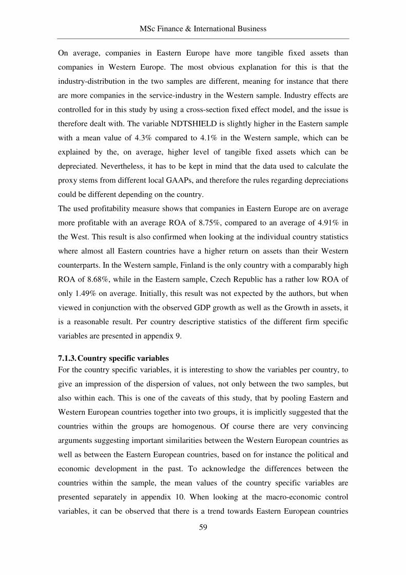
MSc Finance & International Business
59
On average, companies in Eastern Europe have more tangible fixed assets than
companies in Western Europe. The most obvious explanation for this is that the
industry-distribution in the two samples are different, meaning for instance that there
are more companies in the service-industry in the Western sample. Industry effects are
controlled for in this study by using a cross-section fixed effect model, and the issue is
therefore dealt with. The variable NDTSHIELD is slightly higher in the Eastern sample
with a mean value of 4.3% compared to 4.1% in the Western sample, which can be
explained by the, on average, higher level of tangible fixed assets which can be
depreciated. Nevertheless, it has to be kept in mind that the data used to calculate the
proxy stems from different local GAAPs, and therefore the rules regarding depreciations
could be different depending on the country.
The used profitability measure shows that companies in Eastern Europe are on average
more profitable with an average ROA of 8.75%, compared to an average of 4.91% in
the West. This result is also confirmed when looking at the individual country statistics
where almost all Eastern countries have a higher return on assets than their Western
counterparts. In the Western sample, Finland is the only country with a comparably high
ROA of 8.68%, while in the Eastern sample, Czech Republic has a rather low ROA of
only 1.49% on average. Initially, this result was not expected by the authors, but when
viewed in conjunction with the observed GDP growth as well as the Growth in assets, it
is a reasonable result. Per country descriptive statistics of the different firm specific
variables are presented in appendix 9.
7.1.3. Country specific variables
For the country specific variables, it is interesting to show the variables per country, to
give an impression of the dispersion of values, not only between the two samples, but
also within each. This is one of the caveats of this study, that by pooling Eastern and
Western European countries together into two groups, it is implicitly suggested that the
countries within the groups are homogenous. Of course there are very convincing
arguments suggesting important similarities between the Western European countries as
well as between the Eastern European countries, based on for instance the political and
economic development in the past. To acknowledge the differences between the
countries within the sample, the mean values of the country specific variables are
presented separately in appendix 10. When looking at the macro-economic control
variables, it can be observed that there is a trend towards Eastern European countries

MSc Finance & International Business
60
having the highest GDP growth as well as inflation rate. When looking at the stock-
market capitalization to GDP, there is also a rather clear cut distinction between
Western and Eastern Europe, with most Western European countries having higher
values, indicating a higher development of the financial markets. When looking at bank
concentration, the distinction between East and West is not that clear cut, while on
average the bank concentration is higher in the West. On the other hand, when
analyzing the profitability of banks with the variable net interest margin, it can be seen
that there is a strong tendency for banks in Eastern Europe to be more profitable. When
looking at the variable recovery rate, which is an indicator of the quality and
effectiveness of the bankruptcy law, it can be observed that nearly all Western European
countries have higher values than any of the Eastern countries. The only exception is
Lithuania being at Western standards with a value of 50 percent. The variable contract
enforcement is more ambiguous, meaning that while the mean-value in the East is
slightly higher, there is some variation within the different groups. It can for example be
observed that in the Eastern sample, the Baltic countries, Estonia, Latvia and Lithuania
have low (good) contract enforcement values, while Mediterranean countries like Italy,
Greece, Portugal and to a lower extend also Spain, have high (bad) values of contract-
enforcement. This could suggest that cultural commonalities are playing a role in
explaining contract enforcement, and not only whether a country is located in Eastern or
Western Europe. To some extend, national culture, which might have an impact on the
tendency of a company to acquire external financing, is captured in the fixed effect.
Western European countries have in general higher values in the corruption index (less
corruption) than the Eastern European countries. Again, Italy and Greece depart to some
degree from the general tendency, meaning that Estonia actually has a better value in
the corruption index than Italy. This is also the case in terms of Greece, were Hungary,
Lithuania and Estonia have a better value. Taking into consideration the overall picture,
there is however a clear tendency towards higher values in the West compared to East.
When looking at the variables that proxy for credit information, disclosure, investor
protection and legal rights, only for credit-information the values are on average higher
in the West. For the other three variables there is no clear-cut pattern. Some variation is
present within the groups, for instance Great Britain has extraordinarily high values for
disclosure and investor-protection, which could be due to the fact that Great Britain is a
market oriented economy where the majority of the other countries are bank oriented

MSc Finance & International Business
61
(Brounen, Jong & Koedijk 2005). While being interesting to see which sign the
coefficients for these variables have and whether they are statistically significant, the
variation within the groups could potentially have a negative impact on the robustness
of these variables in the model. Taking into account the scope of this paper, which is
among other things to show that country specific factors have an impact on leverage and
that this impact is potentially different between Eastern and Western Europe, this
limitation has to be accepted. Due to data availability on these country specific factors, a
more in-depth segmentation of the countries in more sub-groups is not feasible.
7.2. Regression output
In Table 9 the sign and significance of the coefficients from the regression are presented
separately for each sample. In table 10, the sign and significance of the dummy
interactions are illustrated, showing whether the Eastern sample behaves different from
the Western one. The regression output from Eviews is presented in appendix 11. For
reference, also a regression where Eastern and Western Europe are pooled into one
group is presented in appendix 12. The interpretation is based on the model where
Western Europe serves as the base group and the dummy-interactions represent how and
if the Eastern European sample deviates. Based on this, it is possible to see whether the
Eastern sample behaves different for a specific variable compared to the Western
sample. However, no inference about the significance of the coefficients in the Eastern
European sample can be made from this regression. Therefore a regression for the
Eastern European sample only, is presented in Appendix 13. This regression enables
one to determine the significance of the coefficients in the Eastern sample, and this is
illustrated in the lower part of table 9
The Hausman test presented in appendix 14, confirms that the fixed effects model is the
appropriate specification, while the F-test presented in appendix 15 shows that the fixed
effects are jointly significant.
The effect specifications of the four different regressions all show high R-squared
values, ranging from 0.826 to 0.860 for SHORTBANKDEBT and LONGBANKDEBT
respectively. As has been explained in section 4.1, the high R-squared are as expected
due to the inclusion of a dummy variable for each cross-section.
Serial correlation, meaning that the error terms are correlated over time, does not bias
the coefficient estimates, but can potentially bias the standard errors and therefore the

MSc Finance & International Business
62
associated t-statistics. The presence of serial correlation can be tested using the Durbin-
Watson statistic. A value close to 2.0 indicates that there is no autocorrelation present.
A value considerably smaller would indicate positive autocorrelation, while a value
significantly bigger points toward negative autocorrelation. The actual values of the
Durbin-Watson statistic obtained for the four regressions range from 1.77 for
NARROWLEVERAGE to 1.90 for LONGBANKDEBT. This suggests that there is no
serial correlation.
The issue of potential non constant variance has been addressed by using “White’s
heteroskedasticity robust standard errors”. This issue should therefore not cause any
concern.

MSc Finance & International Business
63
Table 9 – Regression results Western Sample
Shortermdebt shorttermbankdebt narrowleverage longbankdebt
age +*** +*** +*** +***
bankconcentration -*** -*** -*** -***
contractentforcement +*** -*** -*** -***
corruption - +** -*** -***
creditinf -*** -*** - +***
disclosure -*** + -*** -***
gdpgrowth -*** - -*** -***
growthassets -*** -*** +*** +***
inflation -*** -*** + +***
investorprotection +*** +*** +*** +*
legalrights -*** -*** +*** +***
lnturnover +*** +*** +*** +*
marketcaptogdp +*** +*** +*** +*
narrowtangibility -*** -*** +*** +***
ndtshield -*** -*** -*** -***
netinterstmargin +*** +*** +*** +***
recoveryrate -*** -*** -*** +***
roa -*** -*** -*** -***
Eastern sample
shortermdebt shorttermbankdebt narrowleverage longbankdebt
age - -*** -*** -**
bankconcentration -*** -** -*** -
contractentforcement -*** -*** -*** -***
corruption -*** -*** -*** -**
creditinf -*** -*** -*** -
disclosure -*** -*** -*** -***
gdpgrowth -*** - -*** -***
growthassets +*** + +*** +***
inflation +*** +*** +*** +***
investorprotection +*** +*** +*** +***
legalrights - - - -
lnturnover +* +*** + -**
marketcaptogdp +*** +*** +*** +**
narrowtangibility +*** -** +*** +***
ndtshield -* -*** -** -*
netinterstmargin +*** +*** +*** +***
recoveryrate +*** +*** +*** +***
roa -*** -*** -*** -***
* = significant at the 10 % level
** = significant at the 5 % level
***= significant at the 1 % level

MSc Finance & International Business
64
Table 10 – Dummy interactions shortermdebt shorttermbankdebt narrowleverage longbankdebt
age -*** -*** -*** -***
bankconcentration - - - +
contractentforcement -*** -*** -*** +
corruption -*** -*** -*** -
creditinf + - -** -**
disclosure -*** -*** -*** -***
gdpgrowth -*** - +*** +***
growthassets +*** +*** - -**
inflation +*** +*** + -***
investorprotection +*** +*** +*** +***
legalrights + - -* -***
lnturnover -*** -*** -*** -***
marketcaptogdp +*** +*** +*** +***
narrowtangibility -*** + -*** -***
ndtshield +** +** +*** +***
netinterstmargin +*** +*** +*** +***
recoveryrate +*** +*** +*** +**
roa +*** +*** +*** +***
* = significant at the 10 % level
** = significant at the 5 % level
***= significant at the 1 % level
8. Interpretation of results
In the following paragraphs, each hypothesis stated in section 3 will be evaluated based
on the results from the statistical analysis.
8.1. Hypothesis 1 – Leverage in Eastern and Western Europe
It is concluded that there is support for hypothesis 1, namely that leverage is in
general lower in Eastern Europe compared to Western Europe.
The descriptive statistics in table 7 in section 7.1.1 gave an indicator of this, and the
formal statistical test shown in appendix 16, confirms the first hand impression by
showing that there is a significant difference in all four leverage measures between East
and West. This result is confirmed by other studies e.g. (Nivorozhkin 2005) and
(Jõeveer 2005), and is therefore not surprising.

MSc Finance & International Business
65
One thing that was mentioned when describing the descriptive statistics and should be
kept in mind is that the analysis carried out, only shows the difference in average.
Within each group there is some variation, meaning that one cannot interpret the results
as all countries in Western Europe have higher debt ratios than any country in Eastern
Europe.
8.2. Hypothesis 2 – Corporate governance
The regression results only partly support hypothesis 2, that higher levels of corporate
governance are positively related to leverage.
Two measures of corporate governance have been employed in this study, namely
investor protection and disclosure. Investor protection generally shows the results that
were expected, namely a positive coefficient across all leverage measures in both East
and West. Except for LONGBANKDEBT in the Western sample, all coefficients are
significant at the 1%-level. LONGBANKDEBT in West is only significant at the 10%-
level, however with a p-value of 0.059, and is therefore considered to be significant
with fairly strong certainty. This is suggested to clearly indicate that better investor
protection helps SMEs to get credit, both long-term as well as short-term. This goes
well with the static trade-off theory in the sense that agency costs of debt are argued to
decline when investor protection is good. This all else equal increases the level of debt
in the optimal capital structure from the trade-off perspective. The availability of debt is
improved, because for instance the possibility of banks to hold directors personally
liable are improved when investor-protection is high and thereby reduces the
uncertainty of repayment of a loan.
Looking at the dummy interactions in the regressions indicate that the influence of
investor protection is a great deal stronger in the East for all measures of leverage.
Further it looks like trade credits are affected in a similar positive way, since the
coefficient SHORTTERMDEBT is larger than SHORTBANKDEBT in both East and
West.
The fact that East seems to respond more heavily to investor protection than their
Western counterparts can of course stem from several reasons. One reason could be that
banks in the East simply put more weight on investor protection. This could be

MSc Finance & International Business
66
especially important in the East, where corruption is on average higher, see appendix
10. When the probability of corruption is higher, the ability to hold directors personally
liable could be an important tool to restrain managers, and avoid bad behavior. This is
purely a supply side explanation in the sense that it is the banks that are limiting the
credit availability in more corrupt areas if investor protection is not sufficiently good.
Therefore it can be concluded that improved investor-protection has a positive impact
on the availability of debt-financing in Eastern as well as Western Europe, while the
impact is even stronger in Eastern Europe.
The expected positive impact of better corporate governance on leverage is more
ambiguous when looking at disclosure. Quite surprisingly, this proxy has a statistically
significant negative impact on all leverage measures except SHORTBANKDEBT in the
West. The variable was chosen because it was expected to be a proxy for a certain
dimension of the corporate governance system. It results thereby suggest that better
corporate governance should be associated with less debt, which there is no obvious
explanation for. A possible explanation could be that this proxy to a higher degree
proxies for the protection of equity investors. This could mean that a high degree of
disclosure makes equity more available and relatively cheaper; hence debt is not used as
widely. This of cause, strongly contradicts the pecking order theory, and might seem a
bit far fetched, especially when considering that it has been shown that new equity
issues only play a minor role in the capital structure decisions of SMEs. Another and
more plausible reason for the peculiar results regarding the sign of the coefficients,
could be that this variable is not a sufficiently good measure of corporate governance,
and picks up other factors which have not been considered in this study.
To sum up, the argument that better corporate governance has a positive impact on
leverage can only partly be supported, while investor protection supports the hypothesis,
disclosure does not. One possible explanation for the somehow ambiguous results could
be that the employed proxies are not refined enough, and also that not every
improvement of corporate governance, actually leads to improved access to finance.

MSc Finance & International Business
67
8.3. Hypothesis 3 – Legal environment
There is only partly support for hypothesis 3 that a strong legal environment is
positively related to leverage.
The reason for the results only partly supporting the hypothesis is that corruption shows
a negative relation with leverage, which is contrary to what was expected. Again the
reader should keep in mind that a high corruption score means a low degree of
corruption. Contract Enforcement shows the expected sign, and confirms that it is of
importance in determining leverage. Recovery rate also shows the expected sign for all
measures of leverage in the Eastern sample, but only for LONGBANKDEBT in the
Western sample. Finally Legal rights are insignificant in East, while showing negative
and positive signs for short and long-term measures of leverage respectively, in the
west.
Looking more thoroughly at the impact of the proxies on the different leverage
measures, one can see that in the Western sample, recovery rate is negatively related to
SHORTTERMDEBT, SHORTBANKDEBT and NARROWLEVERAGE, while it is
positively related to LONGBANKDEBT. The most negative coefficient is found for
SHORTTERMDEBT, followed by SHORTBANKDEBT. In the Eastern sample,
Recovery rate is positively related to all measures of leverage. All coefficients in the
Western and Eastern samples are significant at the one percent level. The dummy
variable is statistically significant at the one percent level of confidence for all leverage
measures besides LONGBANKDEBT, where it is only significant at the five percent
level of confidence. The coefficients in the Eastern sample are more positive than the
corresponding coefficients in the Western sample, for all measures of leverage.
Recovery rate is a measure for how much creditors can recover in the case of
bankruptcy of the debtor. Hence, it was expected that recovery rate would be positively
related to all measures of leverage, which however is not the case. In the Western
sample, recovery rate is only positively related to LONGBANKDEBT and negatively
related to the rest. The impact and importance of the recovery rate on the propensity of
banks to provide debt-financing, is argued to depend decisively on the probability of
default of the debtor. The probability that a company will default on a short-term loan is

MSc Finance & International Business
68
much smaller than the probability that it will default on a long-term loan. This is due to
the fact that a bank is much more capable to assess the capability of a company to repay
a short-term loan, because the short-term prospects and cash-flows of a company are
much more certain than their long-term prospects and cash-flows. According to this, it
makes sense that the impact of the recovery rate is highest for long-term debt in the
West. The negative relationship between the recovery rate and the short-term debt
measure can be explained as follows: Assuming that recovery rate does not affect the
amount of short-term debt, but does affect the amount of long-term debt and thereby
also increases total assets, given that long-term debt is not taken on to retire short-term
debt, then the short-term debt ratio decreases. In this line of reasoning, the negative
impact on short-term debt actually stems from the impact of long-term debt on the
denominator (total assets) of the short-term leverage measures. The fact that recovery
rate in the East is positively related to all leverage measures, including the ones for
short-term debt, can be seen as a sign of the business environment being more unstable
and volatile in Eastern Europe, meaning that banks consider the possibility of default of
the borrower even when lending short-term. If this is true, it makes sense that a higher
recovery rate will convince more lenders to provide short-term debt or trade credits.
However it is still puzzling that recovery rate is most strongly related to
SHORTTERMDEBT. A possible explanation for this observation is that the proxy
picks up factors that have not been considered by the authors, and therefore further
research is suggested.
The variable contract enforcement is as expected negatively related to all four measures
of leverage in the Eastern sample. The same results are observed for all the leverage
measures but SHORTTERMDEBT in the Western sample. All coefficients are
significant at the one percent confidence level. When comparing the results of the
Eastern sample with the ones from the Western sample, it can be seen that contract
enforcement has an economically higher negative impact on leverage in the Eastern
sample. This is true for all measures of leverage besides LONGTERMBANKDEBT
where no statistically significant difference between the two samples can be identified.
When looking at the Western sample, it can be seen that contract enforcement has the
biggest negative impact on NARROWLEVERAGE, followed by LONGBANKDEBT
and SHORTBANKDEBT, while the smallest economical impact can be observed for

MSc Finance & International Business
69
SHORTTERMDEBT. Looking from the supply-side of bank-credit, it makes sense that
long-term bank debt is more strongly affected by the ease of enforcing a contract than
short-term bank debt. As previously argued, it is easier for a bank to assess the
probability of repayment of a short-term loan. Therefore the importance of the ease to
enforce a claim by legal action increases for a long-term loan because it is more likely
that it becomes necessary to do so, compared to a short-term loan. The supply of long-
term loans should therefore be more negatively affected by long contract enforcement
periods. This line of reasoning is also supported by the fact that SHORTTERMDEBT is
not as strongly affected by long contract enforcement periods as SHORTBANKDEBT
is. The apparent reason here is that the supply of trade-credits is not that much affected
by the length of contract-enforcement, because the probability that it becomes necessary
to enforce the trade-credit by legal action is argued to be smaller, compared to both
short and long-term debt, due to the usually even shorter maturity of trade-credit. The
coefficient on SHORTTERMDEBT suggests that trade-credits are actually positively
related to the length of contract-enforcement. This indicates that companies make more
use of trade-credits when it becomes harder to acquire long and short-term financing.
When comparing the impact of contract enforcement on the different leverage-measure
in Eastern Europe, the picture becomes different. Economically speaking, contract
enforcement has the biggest negative impact on SHORTTERMDEBT, which indicates
that the access to trade-credit as well as short-term debt becomes relatively more
difficult when the time spent to enforce a contract increases. A potential reason for the
fact that contract enforcement is negatively related to trade-credits could be that
repayment behavior concerning trade credits is worse in Eastern Europe. For instance
(Tom 2005) states that the payment behavior of companies in Czech Republic and also
to a lower extend Poland, leaves a lot to be desired. If that is a general pattern, the
probability to have to enforce a claim by legal action is increased, and then it seems
intuitive that a longer processing time of these claims, worsens the access to trade-
credit. The core of this argument is that trade-credit in Eastern Europe is more risky
than it is in Western Europe and is therefore affected by contract enforcement in a
different manner. Contract enforcement also affects SHORTBANKDEBT more
economically significant in Eastern Europe than it does in Western Europe. A potential
explanation could be that default risk on short-term loans is all else equal higher in
Eastern Europe, which is reflected in a higher negative coefficient. To sum up the

MSc Finance & International Business
70
results, it can be noted that in both regions, the ease to enforce a contract is related to
the availability of credit. The explanation for the negative impact of a bad contract
enforcement environment on leverage can only be explained when looking at the
supply-side of debt. Banks take into consideration the ease of recovering their loans
juridical when handing out loans. This seems to be even more important in Eastern
Europe compared to Western Europe.
The proxy for corruption is based on an index from transparency international, where a
higher index value represents less corruption in the country. Therefore a positive
coefficient would mean that all else equal, the less corrupt a country, is the more
leverage a firm in that country is expected to have. In the Western sample the proxy is
statistically insignificant for SHORTERMDEBT and positively related to
SHORTBANKDEBT but only at the five percent significance level. On the other hand
it is negatively related to NARROWLEVERGE and LONGTERMDEBT, both at the
one percent significance level. In the Eastern sample, all leverage measures are
negatively related to corruption at the one percent significance level. In addition the
coefficients of the Eastern sample are all more negative than the corresponding
coefficients in the Western sample. The predominantly negative sign, leads to the
interpretation that the less corrupt a country is the less debt the companies in that
country use. This seems to be counterintuitive at first sight. An explanation for the
result could be that debt is used as a disciplining tool. The corruption index employed
might proxy for the overall propensity of managers to behave unethical. A low value in
the corruption index is also a statement of a countries attitude towards good governance
and what business practices are commonly accepted. If the owner of a company can
expect that the managers of a company do not behave in the best interest of the
company, by for instance making excessive use of perks, it might be reasonable to take
on debt as a disciplining measure. The use of debt as a device to discipline managers
has been stated by Jensen in the so-called “free cash flow hypothesis”. There it is
pointed out that debt has the capability to reduce the agency costs associated with free
cash flows, and can serve to streamline the organization (Jensen 1986). One problem
with this line of reasoning is that many SMEs are managed by the owner, which should
make debt as a restraining measure unnecessary. The detected negative coefficient is

MSc Finance & International Business
71
therefore to some extend puzzling, and the explanation given has to be taken with some
critical skepticism.
The last proxy for the legal environment is Legal Rights. In the Western sample,
LONGBANKDEBT as well as NARROWLEVERAGE shows the expected positive
relation, being significant at the 1%-level. The coefficients are also economically
significant, the values of the index taken into consideration. When turning to the short-
term leverage measures, the picture is different. Here the relationship is negative, also
significant at the 1%-level, however with less economically significant coefficients. In
the East, nothing shows up significant in any of the regressions. This basically suggests
three different relationships depending on leverage measure and region.
One explanation for legal rights to be without importance for leverage in the Eastern
sample could be that it is a bad proxy for the security of lenders in this region, when
employed as a stand-alone measure. As previously argued, this could be due to the
benefits of good legal rights being very much dependent on the enforcement of these
rights. This is what was also described in section 6.2.2.12, and found by (Safavivan,
Sharma 2007). It makes sense that strong legal rights are not worth much if not
enforced. It should be noted that the index is based on whether certain criteria’s are
defined in the law. It is the impression of the authors that the interpretation of laws and
court practice is very important in determining the expected outcome of say a financial
dispute. Therefore the formal definition of some specific rights, may not tell everything
about the actual rights in a country. The insignificant coefficients in the Eastern sample
could be a result of court practice being relatively more important in this region or
enforcement of the law being weaker.
It is challenging to try to explain the sign-change regarding the coefficients on short vs.
long-term debt in the Western sample. Intuitively it seems wrong that better legal rights
should mean that companies have higher difficulties in getting credit, as the coefficients
on SHORTBANKDEBT and SHORTTERMDEBT might suggest when looking at them
isolated. When looking more closely at the two regressions, it can be seen that
SHORTTERMDEBT has a less negative coefficient compared to SHORTBANKDEBT,
meaning that trade credits must pull in the opposite direction i.e. be positively related to
legal rights. Therefore it seems like it is only SHORTBANKDEBT that is negatively
related to legal rights. One interpretation for this is that SHORTBANKDEBT is used as

MSc Finance & International Business
72
a last resort when it is difficult to obtain long-term financing, triggered by weak legal
rights. E.g. it is expected that a company will be more prone to use its overdraft facility
in situations where long-term financing is not possible. This is due to the usually higher
price of an overdraft facility compared to collateral based long-term loans. Since an
overdraft facility is considered a short-term loan, it is included in the
SHORTTERMBANK measure of leverage. If good legal rights ease the availability of
the relatively cheaper long-term financing, it is argued to lower the incentive for using
overdraft facilities and other short-term credit facilities which could be why the negative
coefficient comes up significant.
8.4. Hypothesis 4 – Financial development
Hypothesis 4 that financial development is positively related to firm leverage is to a
large extend supported by the regression results.
The measures used to proxy for financial development are Marketcap to GDP and credit
information. Of these two, Marketcap to GDP is argued to be the most important
measure of financial development in this study. Positive coefficients for Marketcap to
GDP in all regressions across both regions are in accordance with the expected
hypothesis, that a well developed financial market should increase the availability of
credit all else equal. The economical significance turns out to be greater in Eastern
Europe for all leverage measures, and it should also be noted that in the
LONGBANKDEBT regression in West, the statistical significance is somewhat low
with a p-value of 0.086.
An explanation for a positive sign has been presented by (Demirguc-Kunt, Maksimovic
1995), suggesting that a developed stock market helps to convey information from
better informed investors to the market. Thereby it helps to solve the asymmetric
information problem. This explanation does not fit into the context of this research,
since none of the companies in the sample are listed on a stock exchange. Therefore the
answer has to be found somewhere else. In a cross country study (Demirguc-Kunt,
Levine 1995) finds that the stock market development is highly correlated to the
development of the banking market. Assuming this is correct, it makes sense that a
more developed banking market eases the availability of credit for companies. This
could be brought about by developed banking markets being characterized by more

MSc Finance & International Business
73
liquidity, better information flow, better legal environment etc. The general positive
sign is considered intuitive and is not very surprising. A more interesting question arises
from the fact that short-term financing in general, and the companies in the East, turns
out to be more affected. The fact that companies in the East are more affected could
stem from a possible diminishing return from stock market development. That fits with
the results presented in appendix 10 showing that the mean value of market cap to GDP
is lower in East. This is interpreted in the direction that the marginal benefit from an
increase in the financial market development is more beneficial in areas where it is less
developed. Changing relationships depending on the initial development of the stock
market was also found by (Demirguc-Kunt, Maksimovic 1995). In that study the change
is as dramatic as a sign-flip suggesting that in developed markets, further development
decrease the use of equity. The reason that the change is not as dramatic in this study, is
maybe because the companies here do not have the same opportunity for getting
financing through the stock market and thereby substitute this for debt.
Regarding Credit information, the result for LONGBANKDEBT in the Western sample
is statistically but only borderline economically significant, based on the coefficient
being 0.0035 and the highest possible index value being 6. The positive coefficient is as
expected based on the reasoning that a better developed credit information system
should all else equal help creditors in assessing the risk of potential lenders, and thereby
easing SMEs access to credit. By adding the dummy interaction coefficient to the
Western coefficient, it looks like the Eastern sample behaves in the opposite direction
i.e. a negative relation on LONGBANKDEBT. But this can not be confirmed when
turning to the regression performed strictly on the Eastern sample, since the relationship
is not significant (See appendix 13). This result is to some extend surprising, but might
be explained by Eastern European SMEs being additional informational opaque. This
could for instance have the implication that banks do not rely solely on information
from credit registries even if available, but consider it necessary to carry out a thorough
due diligence on the lender, before a loan will be approved. Also the fact that the
companies in East are on average younger, and hence have a shorter and for some
companies insufficient credit history, supports this line of reasoning.
Looking at the other leverage measures, there is a clear trend towards a negative relation
where only the coefficient for NARROWLEVERAGE in the Western sample is
insignificant. This is a result of the two offsetting effects from, the positive coefficient

MSc Finance & International Business
74
on LONGBANKDEBT on the one side, and the negative effect from
SHORTBANKDEBT on the other side. This could suggest a substitution effect of
LONGBANKDEBT for SHORTBANKDEBT. The rationale behind such a substitution
effect based on credit information is nevertheless unclear. From the point of view of the
company, long-term debt is usually more expensive than short-term debt illustrated by
the usually upward sloping yield curve6. The obvious advantage of long-term debt is
that it exposes the company to less refinancing risk. Refinancing risk is however not
considered to be that big of an issue, since it is expected that larger investments are
financed with maturity matched debt. Moreover, larger investments are to a large extend
characterized by being tangible, which is already controlled for in the analysis. Such a
substitution effect meaning that companies take on long-term debt to pay of short-term
debt, stemming from an increase in creditor information, is therefore not expected to be
the case. The SHORTTERMDEBT and SHORTBANKDEBT in both East and West
shows negative coefficients, the former being a lot more economically significant,
suggesting that trade credits are considerably negative related to the development of the
credit information system. This contradicts the expectations and is generally found hard
to explain. It is difficult to think of anything brought about by the presence of credit
registries, that could reduce credit availability or SMEs demand for debt, except
potentially transaction costs. If SMEs in order to get a loan from a bank in the presence
of credit registries have to submit certain information, financial as well as non-financial,
it will add transaction costs to the overall price of the loan making it less attractive.
Here it is reasonable that the effect of these transaction costs is relatively higher on
short-term financing, because these loans are potentially smaller than long-term loans,
while the costs associated with transmitting financial statements to credit-registries is
the same. While this is seen from the demand-side, a possible supply side explanation
also exists. If banks in order to be competitive, perceive it necessary to purchase
information from credit registries if available, and pass on these additional costs to the
clients, it is also going to have an impact on the price of credit and/or the availability
hereof. Summing up, the outcome of the variable was only as expected in the case of
LONGBANKDEBT in the Western sample. For the other cases, possible explanations
have here been argued, but yet they should not be considered definite answers.
6 See e.g. http://www.bloomberg.com/markets/rates/

MSc Finance & International Business
75
Summing up, the hypothesis that financial development is positively correlated to firm
leverage can be supported based on the results from the market-cap to GDP variable.
This measure is in the view of the authors also the most reliable measure for financial
development compared to credit information. The reason is that it is not based on an
index which only covers a narrow area of financial development, but on country specific
data that picks up a broader latitude of financial development. Also when looking at
credit information, the expected result is obtained for LONGBANKDEBT in the West.
It is expected that financial development should be most influential on long-term debt.
Nevertheless it has to be mentioned that the results for the effect of credit information
on the short-term measures of leverage are not clear-cut.
8.5. Hypothesis 5 – Bank concentration
Hypothesis 5 expecting that bank concentration is negatively related to leverage, is
accepted.
This is based on the regression results showing negative coefficients in both regions
across all leverage measures. Only the coefficient on LONGBANKDEBT in the Eastern
sample is insignificant, otherwise the rest is significant at the 1% level except
SHORTTERMDEBT in Eastern Europe, which is significant at the 5% level. These
results are as expected, and provide evidence in favor of the structure-performance
hypothesis, stating that banks are taking advantage of market power by demanding high
prices or by limiting credit availability.
At first sight it might seem surprising that the coefficient for LONGBANKDEBT in the
East is insignificant. The dummy interaction in the pooled regression is not significant,
meaning that it does not prove that the coefficient in the Eastern sample is significantly
different from the one in the Western sample. This would suggest that the coefficients
are fairly equal in the two samples, and it is therefore a good example of the importance
of testing the robustness of the results by running a separate regression on the Eastern
sample. The answer for why the coefficient can neither be tested significantly different
from 0 in the regression only on the Eastern sample, nor significantly different from the
negative coefficient in the Western sample, should be found in the large standard errors.
(Klapper, Sarria-Allende & Sulla 2002) argues that the current financial development
and market structure in Eastern Europe is of a unique nature. This could potentially help

MSc Finance & International Business
76
explain why bank concentration is not significant for LONGBANKDEBT in the East.
The idea is that if the financial infrastructure is still under development, banks in this
region are maybe not to the same extend, able to exploit their market position as
expected by the market power hypothesis. Instead they could be focused on adapting to
the changes in the competitive environment, where foreign banks are expanding their
presence (Clarke et al. 2003). However when looking at the three other measures of
leverage, there is no significant evidence that the relationship is either stronger or
weaker in the Eastern sample i.e. the dummy interaction is insignificant. Bearing in
mind that different measures of bank concentration can lead to contradicting results, and
the difficulties in explaining the insignificant coefficient in the Eastern sample
regarding LONGBANKDEBT, the aggregate results is interpreted in the way of
supporting the structure-performance hypothesis.
8.6. Hypothesis 6 – Bank profitability
Hypothesis 6 that bank profitability is positively correlated to firm leverage is
supported by the regression results.
Net interest margin is as expected positively related to all measures of leverage in both
regions, being significant at the one percent confidence level. Looking at the dummy
representing the Eastern sample, it can be seen that it is always positive and also
significant at the one percent significance level, meaning that net interest margin has a
bigger positive impact on all leverage measures in the Eastern sample.
There are several possible reasons why banking profitability is positively related to
leverage and also to the availability of debt. One reason is that banks that are very
profitable are able to retain more earnings and can thereby improve their equity base.
The profitability and the equity base of a bank, directly influence the rating of the bank.
This rating in turns influences the cost of refinancing for the bank. A bank with a better
rating can refinance itself cheaper and thereby also offer loans at a cheaper rate. This
will increase the demand for bank-credit by SMEs. A related issue is that profitable
banks with a therefore good equity base, can lend out more money. National legislators
limit the amount a bank is allowed to lend to its customers based on the equity base of a
bank. This means that banks are allowed to lend out a multiple of their capital base as

MSc Finance & International Business
77
determined by national regulators. According to the Basel I agreement, which set out
the rules for capital requirement in the EU and the US up to January 1st 2007, banks
which operate internationally are required to hold capital equal to 8 percent of their risk-
weighted assets. It should be noted that Basel I became internationally accepted in the
1990s and has from then on been the standard in roughly one hundred countries. The
risk weights under Basel I was assigned in the following way:
Table 11 – Risk weights under Basel I
Risk weight in % 0 20 50 100
Debtor-category State Bank Mortgages Companies/private customers
This means that a bank with a large equity base which has been acquired for example by
retained earnings can lend more and also take on more risk by lending relatively more to
companies. It has to be noted that one of the main criticisms of Basel I was that it did
not incorporate the creditworthiness of companies into the formula for calculating the
minimum capital requirements, which meant that the same amount of underlying bank-
equity is needed for lending to a company with a high rating as is for lending to a
company with a low rating. This is one of many reasons why new risk-adjusted capital
requirements were introduced within an agreement called Basel II, which became
effective in the EU through the EU-directive 2006/48/EG and 2006/49/EG on the
January 1st 2007 (European Parliament 2006). Under the Basel II regulations there are
now different risk-weights for loans to companies based on their credit rating and hence
the required underlying bank-equity differs depending on this credit rating. This makes
credit more expensive to companies with a low credit-rating in order for the bank to get
the same return on equity, which is in this sense a scarce resource. This study uses data
from the years 2001 to 2006. This means that at this time Basel II was not in effect yet.
This could be an explanation for why bank profitability has a higher impact on leverage
in Eastern Europe than it has in Western Europe, when the expectation is made that
companies in Eastern Europe are on average less creditworthy than firms in Western
Europe. This is due to the fact that there is an incentive for banks to lend to less
creditworthy companies under the regulations of Basel I, because the interest-rates that
can be charged are higher while the necessary underlying equity is the same as for loans
to a company with a better credit rating. So when taking into account that risk is related

MSc Finance & International Business
78
to return, meaning that returns are higher when a bank takes on more risk, it makes
sense that net interest margin has a higher impact on the Eastern sample. An example
clarifying this proposition is presented in Appendix 17. This situation will of course
only prevail as long as taking more risk is profitable for banks. Under Basel II, lending
to companies with a bad credit rating will become more expensive for banks because
these loans have to be backed up with more equity then. Therefore the cost of capital of
lending to companies with a good credit rating is comparably lower. It can therefore be
expected that companies with a bad credit rating will face higher costs for acquiring
debt financing, because the higher costs incurred by the banks will be passed on to the
companies. This expectation would make it very interesting to analyze the impact of
Basel II on SME financing, especially in areas where many companies can expect a
poor credit rating. It would also be interesting to perform a study on the difference
between credit rating in Eastern and Western Europe and to investigate the impact of
bank profitability on leverage under Basel I and how this relationship might change
under Basel II.
8.7. Hypothesis 7 – Eastern and Western Europe respond differently
Hypothesis 7 that companies in the East and West respond differently to country
specific as well as firm specific variables either in strength or sign is supported.
One result of this study, apart from showing that country specific factors do have an
impact on leverage, is that this impact is different when comparing Eastern to Western
Europe for the country specific variables but also for the firm specific variables. This is
regarded as support for hypothesis 7.
When looking at the dummy variables distinguishing the Eastern from the Western
sample, it can be seen that majority is statistically significant. There is only one variable
where the dummy is insignificant for all four leverage measures. This variable is
banking-concentration, indicating that the impact of this variable is not statistically
different between Eastern and Western Europe. Other insignificant dummy variables
can for example be observed for the effect of credit information and legal rights on the
two short-term debt measures. Nevertheless the overall tendency for most variables is
that there are significant differences either in strength or sign.

MSc Finance & International Business
79
Subsequently a discussion of the different variables that have not previously been
discussed will take place, where emphasis will be put on the possible reasons for
differences between the Eastern and the Western sample where applicable.
Firm specific variables
Size
In the Western sample, size behaves as expected and supports by the static trade-off
theory i.e. a positive relation with all leverage measures. This observation fits well with
the general perception that size proxies for the inverse probability of default. Further, as
argued by (Ang, Chua & McConnell 1982), bankruptcy costs are considered to
constitute a relatively larger part of firm value for small firms. In East the coefficient is
insignificant for NARROWLEVERAGE and significantly negative regarding
LONGBANKDEBT, while at the same time being positive for the short-term measures.
Looking at the Western sample first, comparing the regressions show a clear tendency
for the short-term measures of leverage being more affected than LONGBANKDEBT,
in the sense that the size of the coefficients are larger. As previously mentioned, size is
normally argued to proxy for the inverse probability of default. According to this, the
observed difference in impact makes good sense. Bankruptcy costs are not only
determined by the probability of a company going into bankruptcy, but also the costs
that will be incurred during a bankruptcy proceeding. Long-term debt is to a larger
degree expected to be secured by collateral, compared to short-term debt. The implied
cost of bankruptcy for creditors holding collateralized long-term claims is smaller, since
the value of the loan will be backed by an asset, which the creditor have a senior claim
on. Since the value of a collateralized loan should then be less volatile based on
fluctuations in the probability of default, it is argued to be the reason why long-term
debt ratios are not affected to the same degree as short-term debt ratios. It should be
noted that the relation in the LONGBANKDEBT regression is only significant at the
10%-level. But looking at the p-value (0.0555), it shows that it is just on the borderline
of being significant at 5%. The evidence is therefore considered fairly strong.
In all regressions the dummy interactions are significant, showing that the East is
behaving different either in terms of the size of the coefficient or more extremely even
with a sign-change. A sign-change is what is found in the LONGBANKDEBT
regression for the East. The negative coefficient in the East is economically significant

MSc Finance & International Business
80
and statistically significant at the 5%-level. A reverse relationship between regions
regarding size has been seen before e.g. (Rajan, Zingales 1995). They generally find a
positively relation between size and leverage, but surprisingly shows a negative relation
in Germany. They are unfortunately not able to explain this behavior, but suggest
further research. The fact that companies in East seems to have less long-term bank debt
as they grow older, can be seen from both the demand side and the supply side. Seen
from the demand side, the less levered older firms could be a result of their own
preference, while the supply side point of view would suggest that the credit institutions
are responsible for the lack of debt financing. It is not clear why larger firms would
have a preference for smaller debt ratios, but the observed result can stem from larger
firms not being as dependent on debt financing. Larger companies may tend to be more
mature companies with a cash-generating product portfolio i.e. stable cash flows
without the same need to invest heavily in e.g. research and development. By having a
smaller financing need in general, the amount of retained earnings will therefore likely
constitute a relatively larger part of the total financing, thereby bringing down the debt
ratio. This stronger reliance on internal finance points in the direction of the pecking
order theory. However the authors believe that at least to some extend, the answer
should be found on the supply side which will be explained next.
Looking at it from the supply side, the underlying assumption is that companies from
the East have an inferior access to debt-financing compared to the companies in the
West. When companies cannot get sufficient external financing and therefore finance
their operations with retained earnings, it will most likely harm their growth. However
some very successful companies will manage to cope with the financial limitations and
grow larger without using external financing. This could also be a reason among others
why the Western sample is relatively bigger than the Eastern sample i.e. that in the East
lack of availability of debt hinders many companies to reach the threshold for selection
applied in this study. An indicator here fore has been presented by (Klapper, Sarria-
Allende & Sulla 2002) who has identified a very large number of very small companies
in for instance Romania. To some degree this proposition can also be supported by the
fact that on average, Eastern European companies in our sample are almost twice as
profitable as their Western European counterparts. This argument could bring about the
negative relationship between size and leverage. The negative relationship is therefore
suggested to not be brought about by companies paying of debt when they grow older.

MSc Finance & International Business
81
This would also contradict the findings in the West and the vast majority of empirical
research. Instead the unique factors constituting the capital markets in Eastern Europe
potentially restrain the growth of certain companies, resulting in the majority of those
who grow big, to be less levered.
Profitability
As expected, profitability shows a significant negative relationship with all leverage
measures, which is supporting the pecking order theory where more profitable firms use
less debt, because they have more internal funds available. Since this study is only
dealing with SMEs, there is a chance that the manager is also the owner. Considering
this, the question arises about what behavioral pattern is responsible for this negative
relationship. Is the preference for internal funds against external, caused by asymmetric
information, or is it instead rooted in managers wish for retaining control. It is the belief
of the authors that the effect of the latter is definitely not negligible and could very well
count for the majority of the combined effect when talking about SMEs. Looking at the
mathematically construction of the leverage measures, it is clear that even if managers
do not take any actions at all, leverage will decrease as profitable companies are
retaining their earnings.
EF�FG�HF I� JFK -F�L�GF M%� �N OLLF L P
As illustrated above, when a company retains earnings it will increase the asset side of
the balance sheet e.g. by increasing the cash balance, marketable securities etc.
Assuming the company does not use the cash to pay off debt, the passive side of the
balance sheet will only be affected by increasing shareholders funds. In terms of the
leverage measures, the nominator (amount of debt) will stay unchanged, while the
denominator (total assets) will increase, resulting in the leverage measure to decline.
This illustrates that without the management taking any actions regarding debt, the
leverage can decline as a result of increased total assets.
When looking more closely at the regressions, it can be seen that the coefficients are
less economically significant in the LONGBANKDEBT regressions in both East and
West compared to the short-term measures. This suggests that profitability has less to
say in determining long-term debt levels. One explanation for this could be that short-
term debt serves as a buffer and will absorb here and now changes in profitability.

MSc Finance & International Business
82
Long-term debt levels are expected to be more rigid relative to short-term, in the sense
that a firm is not expected to make extraordinary payments on long-term loans, unless it
is perfectly sure that it has enough liquidity for the near future. At the same time,
obtaining long-term financing is costly and will therefore only be taken after a thorough
financial planning process or in connection with a large investment. The point here is
that short-term debt will be used to accommodate the daily liquidity need through e.g.
an overdraft facility because it is more flexible. Cash inflows are likewise expected to
reduce the balance on the overdraft facility as they are incurred, and therefore bringing
down short-term debt. The profitability measure employed here is a somewhat short-
term measure since it goes back only one year. The explanation for the larger impact on
the short-term debt levels is suggested to stem from this type of debt being used as a
liquidity buffer, and is thereby highly dependent on the current profitability of the
company.
Comparing the coefficients between the two regions shows that they are generally less
negative in the East, meaning that these companies respond less to profitability. This
could indicate a finance gap, since profitable companies do not to the same extend as in
the west, substitute debt with internal funds.
Tangibility
In both samples Narrow tangibility is negatively related to SHORTTERMDEBT and
SHORTBANKDEBT, while being positively related to NARROWLEVERAGE and
LONGBANKDEBT. All coefficients are significant at the one percent level of
confidence. When looking at the dummy it can be seen that it is statistically significant
at the one percent level for all four measures of leverage. When comparing the size of
the coefficients of the Eastern Sample with the Western sample, it can be noticed that
the coefficient is higher in the East for SHORTBANKDEBT, while it is higher in the
West for the other three leverage-measures.
The positive impact of narrow tangibility on the long-term leverage measures is as
expected. The reason is that tangible fixed assets can serve as collateral, and therefore
reduce the agency costs of debt (Rajan, Zingales 1995). One reason for the negative
impact of narrow tangibility on the short-term leverage measures is that collateral does
not have the same significance to banks when lending short-term, because they can
more accurately estimate the probability of default. Nevertheless this is not the only

MSc Finance & International Business
83
reason for the negative impact. To fully explain the impact of narrow tangibility on
short-term leverage, one has to look at the way companies finance their investments.
Narrow tangibility is determined as tangible fixed assets over total assets. Tangible
fixed assets contain for instance buildings or machinery. These kinds of capital
investments are expected to usually be financed long-term to achieve maturity-
matching. So when companies make capital investments, they will try to acquire long-
term financing and not short-term financing. Therefore it can be expected for capital
investments, that while total assets increase, short-term debt stays constant, and hence a
negative relationship will be observed (Heyman, Deloof & Ooghe 2003). The more
positive coefficients in the Western sample for the long-term debt measures can
possibly be attributed to the fact that the financial development and also the
enforceability of contracts is in general better in Western Europe. Therefore the relative
value of collateral is improved meaning that in case of default of the debtor, the bank
can easier take hold of the collateral.
Growth
The impact of growth in assets on the different leverage measures is different for the
Eastern and the Western sample. In the Western sample growth in assets is negatively
related to SHORTTERMDEBT and SHORTBANKDEBT, while the former has the
more negative coefficient, implying that not only short-term bank debt, but also trade
credits are negatively influenced by growth. LONGBANKDEBT and
NARROWLEVERAGE are positively related to growth assets. It is clear that the
coefficient on LONGBANKDEBT is bigger than that on NARROWLEVERAGE
because of the negative impact of growth in assets on short-term bank debt, which is
included in the narrow leverage measure. All coefficients for the Western sample are
significant at the one percent significance level. When looking at the dummy variable it
can be seen that in the Eastern sample the impact of growth in assets on the employed
leverage measures is different for all leverages measures, besides
NARROWLEVERAGE. Contrary to the relationship in the Western sample,
SHORTTERMDEBT is positively related to growth in assets in the Eastern sample and
significant at the one percent level. The coefficient for SHORTBANKDEBT has a
positive sign, but is statistically insignificant indicating that the effect observed for
SHORTTERMDEBT stems from trade-credits. The positive sign examined in the

MSc Finance & International Business
84
regressions on NARROWLEVERAGE and LONGBANKDEBT is in line with the
results of the Western sample.
The obtained result for the Western sample is not in line with expectations based on
agency theory, because the sign of growth in assets in the regressions on the two short-
term leverage measures are negative. Myers suggested that the problem of asset
substitution can be resolved with the use of short-term debt to finance growth (Myers
1977), and hence a positive relationship between short-term debt and growth is
expected. To shed light on this effect, the regression result for tangibility, has to be
taken into consideration. As shown above, Tangibility is negatively related to short-term
leverage and positively related to NARROWLEVERAGE and long-term leverage. This
implies that additions to tangible fixed assets are all else equal, financed with long-term
debt. This suggests that companies try to match the maturity of debt to the maturity of
their assets. This result has previously been shown in a study on Belgian SMEs, also
using data from Bureau van Dijk. The same study also proposes that firms with a better
credit-score tend to borrow more long-term, while firms that demonstrate a poor credit
quality borrow short-term (Heyman, Deloof & Ooghe 2003). Maturity matching
provides an explanation for the negative relationship between growth in assets and
short-term debt, as well as for the positive relationship between growth in assets and
long-term debt, i.e. capital investments are financed long-term rather than short-term. If
long-term debt is used to finance capital investments necessary for growth, then total
assets will increase and the short-term debt ration will decrease. Myers’ theory
regarding asset substitution and the connected problem of moral hazard can therefore
not be supported for the Western sample. On the contrary in the Eastern sample, asset
growth is positively related to all measures of leverage but insignificant for
SHORTBANKDEBT. The strongest positive relation in the Eastern sample can be
observed for SHORTTERMDEBT, which would imply that growth is largely financed
with the help of trade-credits. Furthermore the coefficient for LONGBANKDEBT is
higher for the Western sample than it is for the Eastern sample. The proposition is
therefore that companies in the East rely on long-term debt supplemented by trade-
credit to finance growth. In the view of the authors, the reason why trade-credits are
also used to finance growth in Eastern Europe can be attributed to inferior access to
bank-debt compared to Western Europe. This insufficient access to external finance
compared to Western Europe is, as also discussed in section 2.5, supported by a survey

MSc Finance & International Business
85
performed by the European Union as well as by the finding that debt-levels are on
average lower in Eastern Europe compared to Western Europe. It has been suggested
that the access to finance is related to the success of macroeconomic and institutional
reforms, as well as to the development of the capital market in the country (EOS Gallup
Europe 2006) and (Nivorozhkin 2005). The obtained results suggest that companies in
the East as well as in the West, finance growth in assets to some degree with long-term
debt in an effort to match the maturities of debt and assets. This goal is achieved to a
higher degree in the West than in the East, which is believed to be due to financial
constraints in Eastern Europe. No solid evidence supporting Myers’ theory of assets
substitution was found.
Age
Age was expected to be negatively correlated to leverage, based on the belief that older
companies are able to finance a larger part of their investments with funds generated
internally, which is in line with the pecking order theory.
Looking at the model output shows that the Western sample contradicts the expectations
by showing positive coefficients at the 1% level for all 4 leverage measures. The
dummy interaction is significant in all regressions and indicates that the companies in
the Eastern sample respond exactly the other way around i.e. with a negative relation
between age and leverage. This is confirmed when looking at the regressions performed
on only the Eastern sample, except in case of SHORTTERMDEBT, where the variable
is statistically insignificant. Even though it in the expectations was mentioned that the
Eastern sample could behave differently, it is surprising to generally see such a large
difference as a sign shift.
The positive coefficient for West can be interpreted in favor of the static trade-off
theory, while it is hard to explain from the point of view of pecking order theory. In the
framework of static trade-off theory, companies that can show a long credit history
could be associated with less uncertainty since the lender is able to observe how the
company has handled its debt from a historical perspective. Furthermore, older
companies are normally associated with more stable cash flows and are therefore less
risky, which all else equal is argued to ease their access to credit. According to pecking
order theory, older companies have had the opportunity to plow back more retained

MSc Finance & International Business
86
earnings, and therefore should have more internal funds to finance their investments
with, which all else equal is expected to lead to lesser use of debt financing.
One argument why age could be positively related to leverage stems from research on
relationship-lending as also referred to in section 2.7.1.1. It has for instance been shown
that companies that have long-standing relationships with their bank get credit at more
favorable rates. This suggests that older companies that have grown relationships with
their banks for several years have better and also more attractive access to debt-
financing (Santiago Carbó-Valverde, Francisco Rodriquez-Fernandez & Udell 2006). In
a further study, (Booth et al. 2001) states that collateral requirements as well as interest
rates become smaller, the longer the relationship between the company and the bank has
lasted, which is further evidence, pointing towards a positive relation. Moral hazard
problems are also significantly reduced if a company uses the same bank for all their
financial transactions, because the bank can then monitor the companies’ capability to
repay its loans through cash-flow movements on the accounts the company has with the
bank. These arguments could lead to a situation where older firms have more debt than
younger firms, due to better relationships with their bank, which is suggested to result in
better access to debt. Furthermore the positive relationship also fits with the positive
relationship obtained for the size proxy, assuming that both variables are inverse proxies
of default risk, i.e. the availability of debt is higher because the probability of default is
lower.
Regarding the sign shift for the Eastern sample, (Klapper, Sarria-Allende & Sulla 2002)
find a similar negative relation on their sample of Eastern European companies. A
potential explanation for this can be the existence of a similar phenomenon as the one
previously explained in (Pfaffermayr, Stöckl 2008), namely the U-shaped relation
between age and leverage. As can be seen in the descriptive statistics, the companies in
the Eastern sample are in general younger than the companies in the West. This could
suggest a similar U-shape, meaning that in the early years, age is negatively associated
with leverage but the relationship then changes to be positive in the later years. While
this could be due to age only serving as an inverse proxy of default after a critical age
has been reached, it is not possible to say when this sign shift occurs.

MSc Finance & International Business
87
Non debt tax-shield
The results regarding non debt tax-shield generally supports the expectations i.e. a
negative relation with leverage. However the significance levels are different in the two
samples. More precise, the coefficients in the SHORTTERMDEBT and
LONGBANKDEBT regressions are only significant at the 10%-level in the East while
being significant at the 1% level in the West. The negative coefficients across all
leverage measures in both regions provide evidence supporting the trade-off theory. It
means that companies with high tax shields stemming from depreciations are less likely
to utilize debt for tax purposes. Even though it is in line with the trade-off theory, it
does not mean that it contradicts the competing theory of pecking order. Imagine a
company with a given stream of cash flows. If the company for some reason gets an
increase in the non debt tax-shield, the earnings after tax, and thereby all else equal
retained earnings, will increase. This would reduce the need for external financing i.e.
debt, and should therefore result in a smaller debt ratio.
A reason for the LONGBANKDEBT to be less significant in East could stem from the
way the measure is constructed. In this study the non debt tax-shield only takes
depreciation into consideration. (DeAngelo, Masulis 1980) shows that besides
depreciations, factors that can substitute the role of debt for tax purposes can be
research and development costs, investment deductions etc. Without having researched
on the exact tax code of the different countries, it is not possible to argue whether the
ones of Eastern Europe in general gives larger tax advantages in terms of other things
but debt. This could potentially explain why the coefficients are less significant both
economically and statistically in the East. This question is however left for further
research.
Macroeconomic control variables
GDP growth
GDP growth has a negative coefficient for all measures of leverage in both regions. The
measure is not statistically significant for SHORTBANKDEBT in the East as well as in
the West, but for all other leverage measures the coefficients are significant at the one
percent confidence level. There is a significant difference in the behavior of the variable
between East and West for all four employed leverage-measures. For
SHORTBANKDEBT and SHORTTERMDEBT, the coefficient is more negative for the

MSc Finance & International Business
88
Eastern sample while for the other two measures, the coefficient for the west is more
negative. The negative coefficient of this macroeconomic control variable is in
accordance with what was expected.
Inflation
In the Western sample, inflation is positively related to LONGBANKDEBT and is
statistical significant at the one percent level. On the contrary, the effect of inflation on
NARROWLEVERAGE is not statistically significant. This appears to be due to the
offsetting negative effect, inflation has on SHORTBANKDEBT which appears to
cancel out the positive effect on LONGBANKDEBT. Furthermore,
SHORTTERMDEBT has the highest negative coefficient. The dummy variables are all
significant at the one percent level besides the one in the regression on
NARROWLEVERAGE, where it is not statistically significant. In the Eastern sample,
inflation is positively related to all four measures of leverage which is in accordance
with the general expectation. The expectation that inflation is positively related to
leverage is on the one hand based on the fact that (a priori) the “real” cost of debt is
reduced in inflationary periods by deteriorating the real value of the principal. It has
previously been shown (for developed countries) that companies use more debt in
inflationary periods (Modigliani 1983). Furthermore, interest-payments are in fact only
partly true interest payments, while the other part is actually compensation for the loss
of real value of the principal. For tax-purposes, companies are nevertheless able to
deduct their entire interest expenses, including the part which is effectively repayment
of principal. It is interesting to see that the short-term leverage measures are more
positively related to inflation than the long-term leverage measures in the Eastern
sample. There are two possible explanations for this result. When looking at descriptive
statistics, it can be seen that the mean inflation in the East is more than two times bigger
than in the West, with the largest inflation being in Serbia in 2001 with 91.1 percent.
Here it has to be mentioned that in 2001, Serbia was just making the transition to
democracy, and recovering from a war. Nevertheless, very high values of inflation can
be observed for other countries in Eastern Europe as well. Romania for instance
experienced inflation rates of 34.5 percent in 2001, and 22.5 percent in 2002. This leads
to a problem which has been formulated by Mozes in the following way: “There is a
common misconception that in a high inflation environment, long-term investments can

MSc Finance & International Business
89
be funded by long-term loans as long as a high nominal interest rate is charged”
(Mozes 1995, p. 1). From the perspective of the lender, long-term loans in high inflation
environments can yield an acceptable real compensation if the nominal interest rate is
sufficiently high, and the interest-rate risk is managed appropriately. The real cost of the
long-term loan might also be reasonable to the borrower, but it might entail a cash-flow
structure that is unsuitable for financing long-term investments. High nominal interest
rates, make the cash-outflows, stemming from a long-term loan, comparably high in the
early stage of the loan, and could therefore potentially be greater than the expected
cash-inflows from the project at that stage. Capital investments usually require a large
initial cash outlay which has to be recovered over a long period. The inappropriate cash-
flow structure of long-term debt in periods of high inflation might hustle companies
towards taking on short-term debt instead of long-term debt which is supported by the
result for Eastern Europe (Mozes 1995). It has also been shown that in countries with
high inflation the availability of long-term debt from banks, due to the interest-rate risk
encountered by these institutions, is reduced which is further evidence supporting the
observed results (Caprio, Demirgu-Kunt 1998). A reason for the reduced availability of
long-term debt can also be found in the fact that there is a relation between high, and
especially volatile inflation rates, and poor levels of financial development (Boyd,
Levine & Smith 2001). This study employing the variable market-cap to GDP, shows
that good financial development has a positive impact on long-term debt (Demirguc-
Kunt, Thorsten & Levine 2005). The interpretations of the obtained results are
somehow substantiated by the results for the Western sample. Here the impact of
inflation is positive for long-term debt compared to a slightly negative impact on short-
term debt, which indicates that the availability of long-term debt is not that constrained,
because the volatility of inflation rates is smaller and the correlated financial
development is better. Therefore companies are able to make use of the advantages of
inflation on the after-tax costs of debt.
Summing up, there is strong evidence supporting the hypothesis that companies in the
East and West respond differently to country specific variables as well as firm specific
variables either in strength or sign. There are, as discussed above, diverse reasons for
the different impacts of the variables in this study on the employed measures of
leverage, when comparing the Western with the Eastern sample. One interesting point
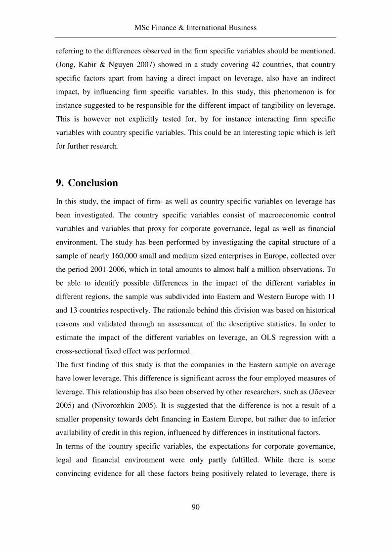
MSc Finance & International Business
90
referring to the differences observed in the firm specific variables should be mentioned.
(Jong, Kabir & Nguyen 2007) showed in a study covering 42 countries, that country
specific factors apart from having a direct impact on leverage, also have an indirect
impact, by influencing firm specific variables. In this study, this phenomenon is for
instance suggested to be responsible for the different impact of tangibility on leverage.
This is however not explicitly tested for, by for instance interacting firm specific
variables with country specific variables. This could be an interesting topic which is left
for further research.
9. Conclusion
In this study, the impact of firm- as well as country specific variables on leverage has
been investigated. The country specific variables consist of macroeconomic control
variables and variables that proxy for corporate governance, legal as well as financial
environment. The study has been performed by investigating the capital structure of a
sample of nearly 160,000 small and medium sized enterprises in Europe, collected over
the period 2001-2006, which in total amounts to almost half a million observations. To
be able to identify possible differences in the impact of the different variables in
different regions, the sample was subdivided into Eastern and Western Europe with 11
and 13 countries respectively. The rationale behind this division was based on historical
reasons and validated through an assessment of the descriptive statistics. In order to
estimate the impact of the different variables on leverage, an OLS regression with a
cross-sectional fixed effect was performed.
The first finding of this study is that the companies in the Eastern sample on average
have lower leverage. This difference is significant across the four employed measures of
leverage. This relationship has also been observed by other researchers, such as (Jõeveer
2005) and (Nivorozhkin 2005). It is suggested that the difference is not a result of a
smaller propensity towards debt financing in Eastern Europe, but rather due to inferior
availability of credit in this region, influenced by differences in institutional factors.
In terms of the country specific variables, the expectations for corporate governance,
legal and financial environment were only partly fulfilled. While there is some
convincing evidence for all these factors being positively related to leverage, there is

MSc Finance & International Business
91
some disturbing evidence regarding certain proxies. It is however beyond doubt that
these three aspects are important in determining leverage of SMEs.
Turning to the proxies for corporate governance, it can be seen that investor protection
shows the expected positive relationship, while disclosure shows a surprising negative
relationship with leverage. On the one hand, this unexpected result supports the
proposition that not every improvement of corporate governance has a positive impact
on debt financing. On the other hand it could show a potential weakness of the index
data, through picking up other effects besides the intended, and thereby not being
refined enough. Based on this, only partly evidence in favor of corporate governance
being positively related to leverage, was found.
There is evidence that the effectiveness of the legal environment is positively associated
with leverage. This is captured by the proxies, contract enforcement and recovery rate.
The legal rights proxy, through being insignificant in the Eastern sample, indicates that
the benefit of a good legal code is very much dependent on effective enforcement. This
is substantiated by the descriptive statistics showing that contract enforcement and
recovery rate are on average worse in Eastern Europe. This line of reasoning is also
suggested by (Safavivan, Sharma 2007). The last proxy concerning the legal
environment is corruption. It was initially expected that less corruption would be
associated with more leverage. The results do however not support this expectation.
Instead it can be seen, that more corruption all else equal leads to more debt among
SMEs. While a potential explanation can be found in the free cash flow hypothesis, this
result is still puzzling, especially when taking into consideration that a non-trivial
amount of SMEs is expected to be owner-managed. Therefore the disciplining function
of debt should be unnecessary.
When looking at the proxies for financial development, it can be seen that the very
broad proxy “Marketcap to GDP” shows the expected result, namely that a more
developed financial environment increases leverage among SMEs. This is interpreted
as an enhancement of credit availability when the overall development of the financial
market increases. Contrary to this intuitive result, the negative impact of credit
information, which is the other proxy for financial development employed in this study,
is challenging to interpret. The negative coefficient could stem from transaction costs
associated with SMEs having to supply credit registries with detailed credit information
when applying for debt financing. However, credit information is picking up a very

MSc Finance & International Business
92
narrow dimension of the degree of financial development, and the overall conclusion is
therefore that financial development is positively associated with leverage of SMEs.
Further, evidence was found supporting that banking concentration is negatively related
to leverage. This is in line with the structure-performance hypothesis, that banks take
advantage of high market power by restraining credit availability and/or increasing the
price of credit.
Banking profitability was shown to have a positive effect on the amount of debt in the
capital structure of SMEs. This is argued to be due to cheaper refinancing possibilities
for profitable banks, and the fact that Basel 1, which was applicable at that time, allows
banks to lend out a certain multiple of their equity base. Profitable banks are assumed to
all else equal increase their equity base, and thereby being able to lend out more money,
which should also be to the benefit of SMEs. Under Basel 1, the credit rating of the
borrower did not affect the amount of equity the bank had to underlie a loan with. With
the implementation of the Basel 2 accords in the beginning of 2007, the amount of
equity a bank has to underlie a loan with is now based on the credit rating of the
borrower. This is suggested to likely harm the credit availability for SMEs, since they
are in general considered to be more risky than for instance large listed companies.
There is in general strong evidence that companies in the two regions respond
differently to country- as well as firm specific variables. This is shown by the majority
of the dummy interactions being significant. The different impact of firm specific
variables can for instance be attributed to country specific factors also having an
indirect impact, through interacting with the firm specific variables. As an example,
tangibility is more economically significant in the West, which could be due to e.g. the
better enforcement of contracts c.f. descriptive statistics. The different impact of country
specific variables can among other things be attributed to elasticity effects, stemming
from the current state of the institutional environment being different in the two regions.
Overall there can be no doubt to the importance of country specific factors in
determining leverage of SMEs. While the static trade-off- and pecking order theory are
useful in explaining the impact of certain firm specific variables on leverage, it has been
beyond the scope of this study to explicitly test which one better explains capital
structure of European SMEs. However it is argued that both models neglect the
importance of the supply side of the financing decision. It has been suggested that

MSc Finance & International Business
93
SMEs, especially in transition economies, are not able to acquire all the financing they
need for pursuing their investment opportunities (OECD 2006). The observation in this
study, that SMEs in the Eastern sample has lower debt ratios, could very well indicate
such a financing gap. OECD has further proposed that the availability of debt financing
is dependent on the development of institutional factors within a country. This study
confirms that, by proving that specific factors related to corporate governance, legal and
financial development are positively correlated to leverage among SMEs.
This is a first attempt to identify relationships between specific institutional factors and
leverage. When further research has confirmed these results, this information can be
very important for policy makers initiating reforms pointed towards enhancing the
environment for SMEs. Especially the fact that the marginal impact of changes in
institutional factors can be different across regions, asks for a careful assessment before
implementation of reforms.
10. Critical assessment and suggestions for further research
The conclusions drawn from this study are based on a thorough analysis. However the
authors are aware of certain weaknesses. While the shortcomings are not considered to
invalidate the overall findings, they should be kept in mind, and are therefore presented
in the following.
Some of the country specific variables used to proxy for institutional factors are based
on index data. This index data is to some degree exposed to subjective judgment about
what factors the index should be based on. E.g. the composition of the determinants of
Investor protection might not reflect all issues of investor protection that could be
relevant to leverage. This means that the indices could potentially pick up unintended
effects. The authors acknowledge this caveat, but were not able to verify the robustness
of the collected indices, based on no data availability from other sources.
The majority of this index data has been gathered and constructed by Doing Business
(the World Bank) which is a fairly new initiative. The fact that these indices are only
available for a narrow timeframe, and that institutional factors do not change very often,
results in moderate intra-country variation. This means that it is not possible to conduct
the study on a “per country” basis. This is the reason why a cross country regression has
been employed. This raises the question of parameter stability within the sample. This

MSc Finance & International Business
94
issue was addressed by subdividing the sample into Eastern and Western Europe. In the
eyes of the authors, this is the most feasible division of these countries, based on a priori
economic expectations and a critical assessment of the descriptive statistics. A formal
cluster analysis has not been performed due to the large number of explanatory
variables. Nevertheless it has to be acknowledged, that a different pooling could
potentially lead to different results.
Another issue is that the coverage of firm specific data from ORBIS is not equally
comprehensive across all countries, stemming from different reporting obligations etc.
This unequal distribution of the sample put some strains on the power of the analysis.
Nevertheless, when sample homogeneity is expected, the severity of this problem is
reduced.
An SME financing gap has been suggested in this paper. This belief rests on evidence
from e.g. the OECD and (Jõeveer 2005). The impact of the country specific factors on
leverage is interpreted as mainly affecting the supply side of financing, and therefore
supports the possibility of a financing gap. It is suggested that further research should be
done regarding the presence and severity of this financing gap. This could for instance
be done through estimating a disequilibrium model as suggested in (Santiago Carbó-
Valverde, Francisco Rodriquez-Fernandez & Udell 2006). Further more, it would be
interesting to shed light on the economic impact of this financing gap and the constraint
on growth.
It has been mentioned that country specific factors do not only have a direct impact on
leverage, but also an indirect effect, through influencing the impact of firm specific
variables. This expectation could be further investigated by including interaction terms
into a regression framework.
In order to surmount the problems associated with evaluating the impact of country
specific variables on leverage through a cross-country study, it would also be very
interesting to perform the analysis on a single country. A potential way to do this could
be, by means of a time-series analysis, where the impact of certain reforms in the
institutional environment over time is assessed. This could also address the issue that
the impact of institutional reforms on leverage is likely to be time-delayed. A potential
drawback of this approach is the possible non-availability of country specific data over
a sufficiently long time-frame especially when index data is used.

MSc Finance & International Business
95
Another important field for further research could be the identification of good proxies
for country specific factors. Many indices are not available for a very long time, or
might lack the necessary refinement for use in an academic study. It would therefore be
very useful to create indices for a longer timeframe in order to make cross country
studies, as well as potentially single country time series analysis, more comprehensive.
A more specific area of further research could be the evaluation of the impact of the
Basel 2 accords on the availability of bank debt to SMEs in Eastern as well as Western
Europe. To the knowledge of the authors, no study has so far compared the credit-
ratings of Eastern European countries with Western European countries.
It would certainly also be interesting to compare the impact of country-specific
variables on leverage, between large listed companies and SMEs. In the view of the
authors it can be expected that the impact on SMEs is larger because they do not to the
same extend have access to international capital markets. Large listed companies can to
some degree, circumvent the effects of country-specific factors through this access
Lastly, it will be interesting to further investigate the impact of institutional reforms on
especially Eastern European SMEs. As mentioned by the World Bank, some countries
in Eastern Europe have introduced massive institutional reforms in the last couple of
years. While the pace of development is not the same across all Eastern European
countries it can be seen that for instance Estonia already have quiet strong institutional
systems. Therefore it needs to be carefully reassessed in the coming years, to what
extend a division of Europe into East and West in respect to capital structure and also
more generally, is still appropriate. In the future, a grouping into Northern and Southern
Europe is maybe more appropriate for a cross-country study like this. An indicator of
this could be that countries like Portugal, Greece and Italy are lacking behind the rest of
Western Europe when it comes to certain institutional factors. This is however only one
possible way of grouping which needs further investigation in the time to come.

MSc Finance & International Business
96
11. Bibliography
Altman, E.I. 1984, "A Further Empirical Investigation of the Bankruptcy Cost
Question", The Journal of Finance, vol. 39, no. 4, pp. 1067-1089.
Ang, J.S., Chua, J.H. & McConnell, J.J. 1982, "The Administrative Costs of Corporate
Bankruptcy: A Note", The Journal of Finance, vol. 37, no. 1, pp. 219-226.
Arellano, C., Bai, Y. & Zhang, J. 2007, Capital Structure and Contract Enforcement,
Federal Reserve Bank of Minneapolis.
Asquith, P. & Mullins, D.J. 1986, "Equity issues and offering dilution", Journal of
Financial Economics, vol. 15, no. 1-2, pp. 61-89.
Auerbach, A.J. 1985, Real Determinants of Corporate Leverage, National Bureau of
Economic Research, Inc.
Baskin, J. 1989, "An Empirical Investigation of the Pecking Order Hypothesis",
Financial Management, vol. 18, no. 1, pp. 26-35.
Beck, T., Demirguc-Kunt, A. & Maksimovic, V. 2004, "Bank Competition and Access
to Finance: International Evidence", Journal of Money, Credit and Banking, vol.
36, no. 3, pp. 627-48.
Berg, S.A. & Kim, M. 1994, "Oligopolistic Interdependence and the Structure of
Production in Banking: An Empirical Evaluation", Journal of Money, Credit and
Banking, vol. 26, no. 2, pp. 309-22.
Berger, A.N. & Udell, G.F. 2006, "A more complete conceptual framework for SME
finance", Journal of Banking & Finance, vol. 30, no. 11, pp. 2945-2966.
Berger, A.N. & Udell, G.F. 2005, A more complete conceptual framework for financing
of small and medium enterprises, World Bank Policy Research Working Paper No.
3795, New York.
Bhaird, Ciarán mac an & Lucey, B. 2007, "Determinants of the Capital Structure of
SMEs: A Seemingly Unrelated Regression Approach", Available at SSRN:
http://ssrn.com/abstract=1018383, .
Bobirca, A. & Miclaus, P. 2007, "Extensiveness and Effectiveness of Corporate
Governance Regulations in South-Eastern Europe", unpublished research paper
available at http://www.waset.org/ijhss/v1/v1-1-2.pdf, .

MSc Finance & International Business
97
Booth, L., Aivazian, V., Demirguc-Kunt, A. & Maksimovic, V. 2001, "Capital
Structures in Developing Countries", The Journal of Finance, vol. 56, no. 1, pp.
87-130.
Bowman, R.G. 1980, "The Importance of a Market-Value Measurement of Debt in
Assessing Leverage", Journal of Accounting Research, vol. 18, no. 1, pp. 242-254.
Boyd, J.H., Levine, R. & Smith, B.D. 2001, "The impact of inflation on financial sector
performance", Journal of Monetary Economics, vol. 47, no. 2, pp. 221-248.
Bradley, M., Jarrell, G.A. & Kim, E.H. 1984, "On the Existence of an Optimal Capital
Structure: Theory and Evidence", The Journal of Finance, vol. 39, no. 3, Papers
and Proceedings, Forty-Second Annual Meeting, American Finance Association,
San Francisco, CA, December 28-30, 1983, pp. 857-878.
Bratkowski, A., Grosfeld, I. & Rostowski, J. 1998, Investment and Finance in De Novo
Private Firms: Empirical Results form the Czech Republic, Hungary and Poland,
DELTA (Ecole normale supérieure).
Brounen, D., Jong, A.d. & Koedijk, C.G. 2005, Capital Structure Policies in Europe:
Survey Evidence, Erasmus Research Institute of Management (ERIM), Rotterdam.
Caprio, G., Jr. & Demirgu-Kunt, A. 1998, "The Role of Long-Term Finance: Theory
and Evidence", The World Bank Research Observer, vol. 13, no. 2, pp. 171-189.
Chaves, R.A., Sanchez, S., Schor, S. & Tesliuc, E. 2001, Financial Markets, Credit
Constraints, and Investment in Rural Romania, World Bank - Technical Papers.
Chen, Y.H. & Hammes, K. 2004, "Capital Structure Theories and Empirical Results - A
Panel Data Analysis", unpublished research paper available at
http://ssrn.com/abstract=535782, .
Cheng, S. & Shiu, C. 2007, "Investor protection and capital structure: International
evidence", Journal of Multinational Financial Management, vol. 17, no. 1, pp. 30-
44.
Chittenden, F., Hall, G. & Hutchinson, P. 1996, "Small firm growth, access to capital
markets and financial structure: Review of issues and an empirical investigation",
Small Business Economics, vol. 8, no. 1, pp. 59-67.

MSc Finance & International Business
98
Clarke, G., Cull, R., Maria Soledad Martinez Peria & Susana M. S·nchez 2003,
"Foreign Bank Entry: Experience, Implications for Developing Economies, and
Agenda for Further Research", World Bank Research Observer, vol. 18, no. 1, pp.
25-59.
Copeland, T.E. 2005, Financial theory and corporate policy Thomas E. Copeland, J.
Fred Weston, 4th ed., Addison-Wesley, Reading, Mass.
Cornelli, F., Portes, R. & Schaffer, M. 1996, The Capital Structure of Firms in Central
and Eastern Europe, DELTA (Ecole normale supérieure).
Corvoisier, S. & Gropp, R. 2002, "Bank concentration and retail interest rates", Journal
of Banking & Finance, vol. 26, no. 11, pp. 2155-2189.
DeAngelo, H. & Masulis, R.W. 1980, "Optimal capital structure under corporate and
personal taxation", Journal of Financial Economics, vol. 8, no. 1, pp. 3-29.
Dell'Ariccia, G. & Bonaccorsi di Patti, E. 2004, "Bank Competition and Firm Creation",
Journal of Money, Credit, and Banking, , no. 01, pp. 225-251.
Demirguc-Kunt, A. & Levine, R. 1995, Stock market development and financial
intermediaries : stylized facts, The World Bank.
Demirguc-Kunt, A. & Maksimovic, V. 1995, Stock market development and firm
financing choices, The World Bank.
Demirguc-Kunt, A., Thorsten, B. & Levine, R. 2005, "Law and Firms' Access to
Finance", American Law and Economics Review, vol. 7, no. 1, pp. 211-252.
Djankov, S., LaPorta, R., Florencio Lopez-de-Silanes & Shleifer, A. 2005, The Law and
Economics of Self-Dealing, National Bureau of Economic Research, Inc.
Djankov, S., McLiesh, C. & Shleifer, A. 2007, "Private credit in 129 countries", Journal
of Financial Economics, vol. 84, no. 2, pp. 299-329.
Egerer, R. 1995, Capital markets, financial intermediaries, and corporate governance :
an empirical assessment of the top ten voucher funds in the Czech Republic, The
World Bank.
EOS Gallup Europe 2006, SME Access to Finance in the New Member States,
European Commision - FLASH EUROBAROMETER.
European Parliament 2006, Directive 2006/49/EC, The European Parliament and the
Council on the capital adequacy of investment firms and credit institutions.

MSc Finance & International Business
99
Fama, E.F. & French, K.R. 2005, "Financing decisions: who issues stock?", Journal of
Financial Economics, vol. 76, no. 3, pp. 549-582.
Fama, E.F. & French, K.R. 2002, "Testing Trade-Off and Pecking Order Predictions
About Dividends and Debt", Review of Financial Studies, vol. 15, no. 1, pp. 1-33.
Fforde, A. 2004, Persuasion: Reflections on Economics, Data and the 'Homogeneity
Assumption', The University of Melbourne.
Fischer, E.O., Heinkel, R. & Zechner, J. 1989, "Dynamic Capital Structure Choice:
Theory and Tests", Journal of Finance, vol. 44, no. 1, pp. 19-40.
Frank, M.Z. & Goyal, V.K. 2007, "Trade-off and Pecking Order Theories of Debt",
Available at SSRN: http://ssrn.com/abstract=670543, .
Frank, M.Z. & Goyal, V.K. 2003, "Testing the pecking order theory of capital
structure", Journal of Financial Economics, vol. 67, no. 2, pp. 217.
Friend, I. & Lang, L.H.P. 1988, "An Empirical Test of the Impact of Managerial Self-
interest on Corporate Capital Structure", Journal of Finance, vol. 43, no. 2, pp.
271-81.
Galpin, N. 2004, "Can the Pecking Order Explain the Costs of Raising Capital?",
unpublished research paper available at
http://papers.ssrn.com/sol3/papers.cfm?abstract_id=475770, .
Giannetti, M. 2000, Do Better Institutions Mitigate Agency Problems? Evidence from
Corporate Finance Choices, Bank of Italy, Economic Research Department.
Graham, J.R. 2000, "How Big Are the Tax Benefits of Debt?", Journal of Finance, vol.
55, no. 5, pp. 1901-1941.
Greene, W.H. 2003, Econometric Analysis, 5th ed., Prentice Hall, New Jersey.
Gual, J. 1999, Deregulation, integration and market structure in European banking,
IESE Business School.
Hall, T.W. & Jörgensen, F. 2006, "Capital Structure, Asset Tangibility, and Creditor
Rights: Time Series Evidence", Research paper available under:
http://www.sse.edu/NR/rdonlyres/58A89700-C377-4705-AE44-
37F98567B6F6/0/FredrikJ%C3%B6rgensen_CreditStructure.pdf, .

MSc Finance & International Business
100
Hall, G.C., Hutchinson, P.J. & Michaelas, N. 2004, "Determinants of the Capital
Structures of European SMEs", Journal of Business Finance & Accounting, vol.
31, no. 5-6, pp. 711-728.
Heyman, D., Deloof, M. & Ooghe, H. 2003, The debt-maturity structure of small firms
in a creditor-oriented environment, Vlerick Leuven Gent Management School.
Hillman, A.L. & Krausz, M. 2005, "Credit markets and corruption", Research Paper
presented at Workshop on “Political Economy and Development”, Available from:
http://www.cesifo-group.de
Jalilvand, A. & Harris, R.S. 1984, "Corporate Behavior in Adjusting to Capital
Structure and Dividend Targets: An Econometric Study", Journal of Finance, vol.
39, no. 1, pp. 127-45.
Jappelli, T. & Pagano, M. 2000, Information Sharing in Credit Markets: The European
Experience, Centre for Studies in Economics and Finance (CSEF), University of
Salerno, Italy.
Jensen, M.C. 1986, "Agency Costs of Free Cash Flow, Corporate Finance, and
Takeovers", American Economic Review, vol. 76, no. 2, pp. 323-29.
Jensen, M.C. & Meckling, W.H. 1976, "Theory of the firm: Managerial behavior,
agency costs and ownership structure", Journal of Financial Economics, vol. 3, no.
4, pp. 305-360.
Jõeveer, K. 2006, Sources of capital structure: evidence from transition countries,
CERGE-EI Working Papers wp306, Prague.
Jõeveer, K. 2005, What Do We Know about the Capital Structure of Small Firms?, The
Center for Economic Research and Graduate Education - Economic Institute,
Prague.
Jong, A.d., Kabir, R. & Nguyen, T.T. 2007, Capital Structure around the World: The
Roles of Firm- and Country-Specific Determinants, Erasmus Research Institute of
Management (ERIM).
Klapper, L., Sarria-Allende, V. & Sulla, V. 2002, Small and medium size enterprise
financing in Eastern Europe, The World Bank.
Lin, C. & Ng, S. 2007, "Estimation of panel data models with parameter heterogeneity
when group membership is unknown", Columbia University publication.

MSc Finance & International Business
101
Lipczynski, J. 2006, Industrial organization an analysis of competing markets
competition, strategy, policy, FT/Prentice Hall, Harlow.
Lopez-Gracia, J. & Sogorb-Mira, F. 2008, "Testing trade-off and pecking order theories
financing SMEs", Small Business Economics, , no. vol. 31(2), pp. 117-136.
Lucey, B. & Bhaird, Ciarán mac an 2006, "What Determines the Capital Structure of
SMEs: Irish Evidence", Available at SSRN: http://ssrn.com/abstract=905845, .
MacKie-Mason, J.K. 1990, "Do Taxes Affect Corporate Financing Decisions?", The
Journal of Finance, vol. 45, no. 5, pp. 1471-1493.
Mcgee, R.W. & Preobragenskaya, G.G. 2004, "Corporate Governance In Transition
Economies: The Theory And Practice Of Corporate Governance In Eastern
Europe", unpublished research paper available at
http://papers.ssrn.com/sol3/papers.cfm?abstract_id=538582, .
Michaelas, N., Chittenden, F. & Poutziouris, P. 1999, "Financial Policy and Capital
Structure Choice in U.K. SMEs: Empirical Evidence from Company Panel Data",
Small Business Economics, vol. 12, no. 2, pp. 113-130.
Modigliani, F. 1983, "Debt, Dividend Policy, Taxes, Inflation, and Market Valuation:
Erratum", Journal of Finance, vol. 38, no. 3, pp. 1041-1042.
Modigliani, F. & Merton H. Miller 1963, "Corporate Income Taxes and the Cost of
Capital: A Correction", The American Economic Review, vol. 53, no. 3, pp. 433-
443.
Modigliani, F. & Merton H. Miller 1958, "The Cost of Capital, Corporation Finance and
the Theory of Investment", The American Economic Review, vol. 48, no. 3, pp.
261-297.
Mozes, D. 1995, Long-term finance in inflationary economies: high inflation creates
punishing repayment schedules, the Worldbank - technical note FPD note Nr. 35.
Myers, S.C. 2001, "Capital Structure", Journal of Economic Perspectives, vol. 15, no. 2,
pp. 81-102.
Myers, S.C. 1984, "The Capital Structure Puzzle", Journal of Finance, vol. 39, no. 3,
pp. 575-92.
Myers, S.C. 1977, "Determinants of corporate borrowing", Journal of Financial
Economics, vol. 5, no. 2, pp. 147-175.

MSc Finance & International Business
102
Nivorozhkin, E. 2005, "Financing choices of firms in EU accession countries",
Emerging Markets Review, vol. 6, no. 2, pp. 138-169.
OECD (ed) 2006, The SME financing gap - Theory and Evidence, Volume 1 ed.,
OECD Publishing, Paris.
Ou, C. & Haynes, G. 2006, "Acquisition of Additional Equity Capital by Small Firms
– Findings from the National Survey of Small Business Finances", Small
Business Economics, vol. 27, no. 2, pp. 157-168.
Pagano, M. & Jappelli, T. 1993, "Information Sharing in Credit Markets", Journal of
Finance, vol. 48, no. 5, pp. 1693-1718.
Petersen, M.A. & Rajan, R.G. 1995, "The Effect of Credit Market Competition on
Lending Relationships", The Quarterly Journal of Economics, vol. 110, no. 2, pp.
407-43.
Pfaffermayr, M. & Stöckl, M. 2008, "Capital Structure, Corporate Taxation and Firm
Age", Working Paper from Faculty of Economics and Statistics, University of
Innsbruck, .
Porta, R.L., Florencio Lopez-de-Silanes, Shleifer, A. & Vishny, R.W. 1998, "Law and
Finance", Journal of Political Economy, vol. 106, no. 6, pp. 1113-1155.
Prasad, S., Green, C.J. & Murinde, V. 2001, Company Financing, Captial Structure, and
Ownership: A Survey, and Implications for Developing Economies, SUERF - The
European Money and Finance Forum.
Quantitative Micro Software (ed) 2005, Eviews 5.1 update, 3.th edn, Irvine, Canada.
Quantitative Micro Software (ed) 2004, Eviews 5 User's guide, Irvine, Canada.
Rajan, R.G. & Zingales, L. 1995, "What Do We Know about Capital Structure? Some
Evidence from International Data", Journal of Finance, vol. 50, no. 5, pp. 1421-
1460.
Roberts, M.J. 1984, "Testing oligopolistic behavior", International Journal of Industrial
Organization, vol. 2, no. 4, pp. 367-383.
Safavivan, M. & Sharma, S. 2007, "When Do Creditor Rights Work?", Available at
SSRN: http://ssrn.com/abstract=953009, .
Santiago Carbó-Valverde, Francisco Rodriquez-Fernandez & Udell, G.F. 2006, "Bank
market power and SME financing constraints", Proceedings, , pp. 143-163.

MSc Finance & International Business
103
Shenoy, C. & Koch, P.D. 1996, "The firm's leverage-cash flow relationship", Journal of
Empirical Finance, vol. 2, no. 4, pp. 307-331.
Shyam-Sunder, L. & Myers, S.C. 1999, Testing static trade-off against pecking-order
models of capital structure, National Bureau of Economic Research, Inc.
Sogorb-Mira, F. 2005, "How SME Uniqueness Affects Capital Structure: Evidence
From A 1994-1998 Spanish Data Panel", Small Business Economics, vol. 25, no. 5,
pp. 447-457.
Thies Clifford F & Klock Mark S 1992, "Determinants of capital structure", Review of
Financial Economics, vol. 1, no. 2, pp. 40-53.
Titman, S. & Wessels, R. 1988, "The Determinants of Capital Structure Choice",
Journal of Finance, vol. 43, no. 1, pp. 1-19.
Tom, D. 2005, "Steady Economic Progress In Central And Eastern Europe", Business
Credit, vol. 107, no. 6, pp. 54-57.
Vliegenhart, A. & Horn, L. 2007, "The Role of the EU in the (Trans)formation of
Corporate Governance Regulation in Central Eastern Europe - The Case of Czech
Republic", unpublished research paper available at
http://www.ingentaconnect.com/content/maney/com/2007/00000011/00000002/art0
0004, .
Wald, J.K. 1999, "How Firm Characteristics Affect Capital Structure: An International
Comparison", Journal of Financial Research available at SSRN:
http://ssrn.com/abstract=142576, .
Warner, J.B. 1977, "Bankruptcy, absolute priority, and the pricing of risky debt claims",
Journal of Financial Economics, vol. 4, no. 3, pp. 239-276.
Weston, F.J. 1955, "Toward Theories of Financial Policy", The Journal of Finance, vol.
2.
Williams, J.B. 1938, "The Theory of Investment Value", Harvard University Press, .
Wooldridge, J.M. 2006, Introductory Econometrics, a modern approach, 3.th edn,
Thomson, Mason, USA.
World Bank "Doing Business 2008", Available at www.doingbusiness.org, .

MSc Finance & International Business
104
12. Appendices – Table of contents
Appendix 1: Risk Shifting I
Appendix 2: Institutional factors in Eastern and Western Europe II
Appendix 3: Country Risk V
Appendix 4: Regression equation VI
Appendix 5: The special case of collecting data in 2001 and 2002 VII
Appendix 6: Regression output for Current Liabilities and Broadleverage VIII
Appendix 7: Empirical Evidence on firm specific variables X
Appendix 8: Per country descriptive statistics of the leverage measures XIV
Appendix 9: Per country descriptive statistics of firm specific variables XV
Appendix 10: Mean values of country specific factors per country XVI
Appendix 11: Regression output XVIII
Appendix 12: Pooled regression XXII
Appendix 13: Regression for the Eastern European sample only XXIII
Appendix 14: Hausmann test XXV
Appendix 15: F-test for joint significance of the fixed effects XXVI
Appendix 16: Equality test of leverage XXVII
Appendix 17: Example on Net interest margin XXVIII

MSc Finance & International Business
I
Appendix 1 - Risk shifting
Overall project Shareholder payoff Debt holder payoff
125
75
50
Low volatility E(V) = 100 E(V) = 50 E(V) = 50
75 25 50
175
125
50
High volatility E(V) = 100 E(V) = 62.5 E(V) = 37.5
25 0 25 Assumption: Initial project is financed with 50 in equity and 50 in debt. Probability of good/bad scenario is 50%
The above figure shows how shareholders can extract wealth from the debt holders by undertaking
a more volatile project, after receiving debt financing.
The first column named “Overall project”, shows the two different projects that the company can
invest in. Both projects have an expected value of 100, but the risk is different, illustrated by the
different cash flows in the good and bad states. Moving to the right, the next column shows
shareholders payoff in good and bad states, along with the expected value from their perspective.
Shareholders payoff in a specific state is computed by subtracting the debt (equal to 50) from the
cash flow of the overall project in the equivalent state. The last column shows the payoff to debt
holders. They have a promised payoff of 50, which they will exactly get in all states, except if the
company defaults on the debt i.e. the cash flow from the overall project is not sufficient.
If the company undertakes the low volatility project, then the value of the shareholders stake in the
company is 50, as seen by the expected value. Similarly, debt holders get 50, and thereby the
overall project value of 100 is equally split between the two.
Now if the company undertakes the high volatility project the expected value of the overall project
is still 100. Shareholders can however see the value their stake, increase to 62.5 while debt holders
will see the value of their claim diminishing.

MSc Finance & International Business
Appendix 2 – Institutional factors in Eastern and
Corporate governance is in many Eastern European countries a fairly new
the Berlin Wall and the collapse of the Soviet Union, corporate governance was not an issue since
companies were owned by the state. After this, things have changed in the old East block.
Companies have been privatized, capital m
corporate governance has become important in order to attract external capital
Preobragenskaya 2004). The need for good corporate governance in the
even more important than in the West, because they do not have the long established financial
infrastructure to monitor corporations and take care of corporate governance issues, as argued by
(Bobirca, Miclaus 2007). In line with the general perception,
Corporate Governance in Eastern Europe is on average
the fact that the systems are still young.
In order to verify that, data on different country specific measures from a sample of
Western countries has been collected and presented below in order to give a general overview.
Credit-information, investor-protection, legal rights and corruption are index data, while market cap
to GDP is a ratio. For all these measure a high value is better. Contract enforcement is measured in
years, and a smaller value is therefore better
0,00
2,00
4,00
6,00
8,00
MARKETCAPTOGDP CREDITINF
Western Europe
Western Europe: Austria, Belgium, Switzerland, Ge
Greece, Italy, Netherlands, Portugal and Sweden.
Eastern Europe: Bulgaria, Czech Republic, Estonia, Croatia, Hungary, Lithuania, Latvia, Poland,
Romania, Serbia and Slovakia
Source: Doingbusiness.org and GMID,
MSc Finance & International Business
II
Institutional factors in Eastern and Western Europe
Corporate governance is in many Eastern European countries a fairly new issue. Before the fall of
the Berlin Wall and the collapse of the Soviet Union, corporate governance was not an issue since
companies were owned by the state. After this, things have changed in the old East block.
Companies have been privatized, capital markets have evolved, and suddenly the issue of good
corporate governance has become important in order to attract external capital
. The need for good corporate governance in the Eastern
even more important than in the West, because they do not have the long established financial
infrastructure to monitor corporations and take care of corporate governance issues, as argued by
. In line with the general perception, (Bobirca, Miclaus
ernance in Eastern Europe is on average lagging behind, as a natural consequence of
young.
In order to verify that, data on different country specific measures from a sample of
countries has been collected and presented below in order to give a general overview.
protection, legal rights and corruption are index data, while market cap
to GDP is a ratio. For all these measure a high value is better. Contract enforcement is measured in
is therefore better.
INV. PROTECTION LEGALRIGHTS CORRUPTION CONTRACTENF
Western Europe Eastern Europe
Europe: Austria, Belgium, Switzerland, Germany. Spain, Finland, France, Great Britain,
Greece, Italy, Netherlands, Portugal and Sweden.
Eastern Europe: Bulgaria, Czech Republic, Estonia, Croatia, Hungary, Lithuania, Latvia, Poland,
Source: Doingbusiness.org and GMID, Average values from 2001-2006
Europe
issue. Before the fall of
the Berlin Wall and the collapse of the Soviet Union, corporate governance was not an issue since
companies were owned by the state. After this, things have changed in the old East block.
and suddenly the issue of good
corporate governance has become important in order to attract external capital (Mcgee,
Eastern countries is maybe
even more important than in the West, because they do not have the long established financial
infrastructure to monitor corporations and take care of corporate governance issues, as argued by
(Bobirca, Miclaus 2007) finds that
lagging behind, as a natural consequence of
In order to verify that, data on different country specific measures from a sample of Eastern and
countries has been collected and presented below in order to give a general overview.
protection, legal rights and corruption are index data, while market cap
to GDP is a ratio. For all these measure a high value is better. Contract enforcement is measured in
CONTRACTENF
Spain, Finland, France, Great Britain,
Eastern Europe: Bulgaria, Czech Republic, Estonia, Croatia, Hungary, Lithuania, Latvia, Poland,

MSc Finance & International Business
III
The graph is intended to confirm the perception that Western European countries are generally
speaking on a higher level of development, but at the same time raise the question whether it in the
future will still be correct to talk about the East and West as two separate blocks of countries.
Looking at the graph gives a good grasp of the current situation and shows that the West is on
overall more developed. But it is also clear that at least parts of Eastern Europe are catching up on
certain aspects, like for instance investor protection and legal rights, as can be seen in the graph and
also from the appendix 3. One can for instance mention Estonia which is a good example of an
Eastern European country with consistently high GDP growth rates which can at least partly be
attributed to the good institutional reforms in the country. Regarding investor protection and legal
rights, it is however important to keep in mind that e.g. good legal rights has to be enforced in order
to be effective. Investor protection and legal rights in this graph only tells something about the
presence of certain rights in the law, but not the strength of the legal system in general.
Financial development proxied by market cap to GDP, shows the most clear cut difference between
East and West. Also when turning to corruption, which is argued to be a crucial factor, the East has
room for improvement. Credit Information which is another variable related to the development of
financial markets is also indicating that the West is more developed.
On certain aspects of corporate governance like investor protection and legal rights, it is however
not possible to make a clear-cut distinction. This is argued to be due to two things. First, some
countries in Western Europe e.g. Greece and Italy are lacking behind the rest of Western Europe
regarding a few factors, and are thereby dragging down the average score. Secondly, and this is
most likely the most important thing. Eastern Europe has in the later period being among the top
reformers in the world (World Bank). This has as a result helped several of the countries to improve
the environment for doing business, bringing it closer to Western standards.
It is argued that the EU used to, and still plays an important role in the development and
transformation of corporate governance systems in the East. Czech Republic serves as a good
example for this importance. In Czech Republic’s process toward accession into the European
Union, the EU was exporting a political agenda that set out to regulate markets and improve the
overall corporate governance in the country (Vliegenhart, Horn 2007). One of the initiatives was to
privatize the banking sector, which together with a more developed capital market, is argued to
attract foreign capital, which in turn demands for better corporate governance (Vliegenhart, Horn
2007). The acceptance of the new EU member states will likely put pressure on these to enhance
their corporate governance system as well as financial development. This will possibly lead to a

MSc Finance & International Business
IV
further convergence between countries in the EU. Since some of the Mediterranean countries in
Western Europe are not performing as good as the rest of the Western countries, there is a danger
that they will lack behind some of the new economies in the future, if they do not improve.
Summing up, it might be valid to talk about East and West right now, but in the future the picture
could become more blurred.

MSc Finance & International Business
V
Appendix 3 - Country Risk
The country-risk measures have been obtained from www.country-check.com, which is a project of
the World-check. World-check is one of the leading providers of risk intelligence in the world.

MSc Finance & International Business
VI
Appendix 4 - Regression equation
The equation below the one estimated in Eviews:
LEVERAGE = C(1) + C(2)*AGE + C(3)*AGE*DUMMY + C(4)*BANKCONCENTRATION
+ C(5)*BANKCONCENTRATION*DUMMY + C(6)*CONTRACTENF +
C(7)*CONTRACTENF*DUMMY + C(8)*CORRUPTION + C(9)*CORRUPTION*DUMMY
+ C(10)*CREDITINF + C(11)*CREDITINF*DUMMY + C(12)*DISCLOSURE +
C(13)*DISCLOSURE*DUMMY + C(14)*GDPGROWTH + C(15)*GDPGROWTH*DUMMY
+ C(16)*GROWTHASSETS + C(17)*GROWTHASSETS*DUMMY + C(18)*INFLATION +
C(19)*INFLATION*DUMMY + C(20)*INVESTORPROTECTION +
C(21)*INVESTORPROTECTION*DUMMY + C(22)*LEGALRIGHTS +
C(23)*LEGALRIGHTS*DUMMY + C(24)*LNTURNOVER +
C(25)*LNTURNOVER*DUMMY + C(26)*MARKETCAPTOGDP +
C(27)*MARKETCAPTOGDP*DUMMY + C(28)*NARROWTANGIBILITY +
C(29)*NARROWTANGIBILITY*DUMMY + C(30)*NDTSHIELD +
C(31)*NDTSHIELD*DUMMY + C(32)*NETINTERESTMARGIN +
C(33)*NETINTERESTMARGIN*DUMMY + C(34)*RECOVERYRATE +
C(35)*RECOVERYRATE*DUMMY + C(36)*ROA + C(37)*ROA*DUMMY

MSc Finance & International Business
VII
Appendix 5 – The special case of collecting data in 2001 and 2002
When it comes to collecting data for 2001 and 2002, it is not possible in the ORBIS search interface
to apply the SME filter for these years. The reason for this is that it unfortunately is not possible to
specify search criteria’s for data prior to 2003.
This issue was dealt with by applying the SME filter so as the companies fulfill it in year 2003, but
adding some slack in both ends of the intervals in order for allowing companies to have changed
their status since the year of interest. The used criteria’s can be seen in the table below, which for
total assets and revenue is the equivalent of adding/subtracting 25% in each end, and for employees
expanding the interval to all companies with up to 350 employees, compared to the SME filter used
for the other years.
Search criteria’s for 2001 and 2002
Total Assets 1.5 M. € ≤ 53.75 M. €
Revenue 1.5 M. € ≤ 62.5 M. €
Employees 1 ≤ 350
After this search, the data were sorted in Excel in order to filter out companies who did not fulfill
the correct SME criteria’s for 2001 and 2002.
This way of identifying SMEs in 2001 and 2002 is of course not optimal, but is considered to be a
fair way of coping with the problem of specifying criteria’s for the years prior to 2003. This is due
to the data for these years only being considered slightly biased in terms of survivorship. This is
argued to be the case because the time difference is only 1 and 2 years respectively, so the number
of companies being kept out of the sample in the 2 years because of bankruptcy in a later year
should be very small.

MSc Finance & International Business
VIII
Appendix 6 – Regression output for Current Liabilities and Broadleverage
BROADLEVERAGE CURRENTLIABILITIES
Variable Coefficient t-Statistic p-value Coefficient t-Statistic p-value
C 0.544875 40.95203 0.0000 0.236587 16.26893 0.0000
AGE -0.008003 -50.54367 0.0000 -0.009673 -57.57299 0.0000
AGE*DUMMY 0.003879 3.851842 0.0001 0.007028 9.355788 0.0000
BANKCONCENTRATION -0.03165 -18.72651 0.0000 -0.0069 -3.533217 0.0004
BANKCONCENTRATION*DUMMY 0.089434 6.154233 0.0000 0.055726 3.538776 0.0004
CONTRACTENF -0.000152 -17.95902 0.0000 -5.72E-05 -5.834278 0.0000
CONTRACTENF*DUMMY -9.46E-05 -2.337623 0.0194 -0.000144 -3.556336 0.0004
CORRUPTION 0.004538 5.060028 0.0000 0.016454 16.47227 0.0000
CORRUPTION*DUMMY -0.042662 -8.987829 0.0000 -0.048052 -9.925184 0.0000
CREDITINF 0.010159 7.558801 0.0000 0.007783 5.072618 0.0000
CREDITINF*DUMMY -0.023315 -7.933174 0.0000 -0.021927 -7.263715 0.0000
DISCLOSURE -0.000755 -1.713366 0.0866 0.005127 10.92427 0.0000
DISCLOSURE*DUMMY -0.052069 -7.883944 0.0000 -0.06012 -7.887215 0.0000
GDPGROWTH -0.00176 -7.116468 0.0000 0.003283 11.83396 0.0000
GDPGROWTH*DUMMY 0.0008 1.087255 0.2769 -0.002986 -3.53918 0.0004
GROWTHASSETS 0.037079 52.61015 0.0000 0.028728 35.71632 0.0000
GROWTHASSETS*DUMMY -0.004935 -2.208572 0.0272 -0.00462 -1.82749 0.0676
INFLATION 0.003943 9.028658 0.0000 -0.002813 -6.348211 0.0000
INFLATION*DUMMY -0.003581 -7.824476 0.0000 0.003412 7.318107 0.0000
INVESTORPROTECTION -0.001058 -3.326248 0.0009 0.000197 0.462973 0.6434
INVESTORPROTECTION*DUMMY 0.042668 2.021863 0.0432 0.047619 2.08976 0.0366
LEGALRIGHTS 0.002043 2.406966 0.0161 0.00143 1.610502 0.1073
LEGALRIGHTS*DUMMY 0.01879 2.277877 0.0227 0.032305 3.706914 0.0002
LNTURNOVER 0.04546 45.02174 0.0000 0.054644 49.00926 0.0000
LNTURNOVER*DUMMY -0.011493 -3.060687 0.0022 -0.023507 -5.772433 0.0000
MARKETCAPTOGDP 0.000736 0.538262 0.5904 -0.001527 -1.107258 0.2682
MARKETCAPTOGDP*DUMMY -0.165107 -8.440041 0.0000 -0.14744 -8.305126 0.0000
NARROWTANGIBILITY -0.014598 -4.349368 0.0000 -0.25407 -68.12744 0.0000
NARROWTANGIBILITY*DUMMY -0.058704 -3.982305 0.0001 -0.036005 -2.308714 0.0210
NDTSHIELD -0.086894 -5.393873 0.0000 -0.002106 -0.125979 0.8997
NDTSHIELD*DUMMY 0.010277 0.231386 0.8170 -0.04793 -1.365354 0.1721
NETINTERESTMARGIN 0.308172 11.02949 0.0000 -0.002514 -0.080309 0.9360
NETINTERESTMARGIN*DUMMY 0.928474 4.674462 0.0000 1.272306 5.725902 0.0000
RECOVERYRATE -1.49E-06 -0.057388 0.9542 -0.000311 -11.06551 0.0000
RECOVERYRATE*DUMMY 0.001215 5.951133 0.0000 0.001181 5.739573 0.0000
ROA -0.004597 -89.56732 0.0000 -0.003193 -63.1101 0.0000
ROA*DUMMY 0.000203 1.317626 0.1876 -6.08E-05 -0.398009 0.6906

MSc Finance & International Business
IX
Effects Specification Effects Specification
Cross-section fixed effect Cross-section fixed effect
R-squared 0.937211 R-squared 0.914057
Adjusted R-squared 0.907263 Adjusted R-squared 0.873081
S.E. of regression 0.07008 S.E. of regression 0.083655
Sum squared resid 1624.754 Sum squared resid 2315.904
Log likelihood 700768.8 Log likelihood 614334.5
Durbin-Watson stat 1.621983 Durbin-Watson stat 1.937125
Mean dependent var 0.692523 Mean dependent var 0.541041
S.D. dependent var 0.230126 S.D. dependent var 0.234816
Akaike info criterion -2.222483 Akaike info criterion -1.868399
Schwarz criterion 1.361888 Schwarz criterion 1.715069
F-statistic 31.29457 F-statistic 22.30748
Prob(F-statistic) 0 Prob(F-statistic) 0

MSc Finance & International Business
X
Appendix 7 – Empirical evidence on firm specific variables
This appendix presents five tables from (Prasad, Green & Murinde 2001). The tables are intended to
give an overview of some of the empirical work that has been done on capital structure
incorporating the same firm specific variables as in this paper (except age). The tables show the
estimated relationship between the applied proxy and leverage. In order to obtain detailed
references, the reader must turn to the original source (Prasad, Green & Murinde 2001).
Table 1: The Influence of Tangibility on Firm Leverage
Source: (Prasad, Green & Murinde 2001)

MSc Finance & International Business
XI
Table 2: The Influence of Size on Firm Leverage
Source: (Prasad, Green & Murinde 2001)

MSc Finance & International Business
XII
Table 3: The Influence of Profitability on Firm Leverage
Source: (Prasad, Green & Murinde 2001)

MSc Finance & International Business
XIII
Table 4: The Influence of Growth on Firm Leverage
Source: (Prasad, Green & Murinde 2001)
Table 5: The Influence of Non-debt Tax-shields on Firm Leverage
Source: (Prasad, Green & Murinde 2001)

MSc Finance & International Business
XIV
Appendix 8 - Per country descriptive statistics of the leverage measures
Western Europe
SHORTTERMDEBT SHORTBANKDEBT NARROWLEVERAGE LONGBANKDEBT
Austria 0.209219 0.107058 0.351426 0.244367
Belgium 0.347052 0.090384 0.216822 0.126439
Switzerland 0.105516 0.03398 0.312323 0.278342
Germany 0.252077 0.110686 0.318816 0.20813
Spain 0.184611 0.065196 0.203473 0.138276
Finland 0.177956 0.056096 0.250623 0.194527
France 0.32945 0.075436 0.097644 0.022208
Great Britain 0.317848 0.127264 0.245074 0.11781
Greece 0.484531 0.226481 0.286143 0.059662
Italia 0.393845 0.147647 0.204875 0.057228
Netherlands 0.230834 0.095375 0.178067 0.082692
Portugal 0.352476 0.12348 0.279394 0.155914
Sweden 0.168945 0.03252 0.222837 0.190317
Eastern Europe
SHORTTERMDEBT SHORTBANKDEBT NARROWLEVERAGE LONGBANKDEBT
Bulgaria 0.373192 0.072366 0.261077 0.188711
Czech Republic 0.261357 0.063792 0.128589 0.064797
Estonia 0.301823 0.097549 0.225317 0.127768
Croatia 0.41631 0.098441 0.098441 0
Hungary 0.17887 0.06674 0.093691 0.025305
Lithuania 0.360198 0.109521 0.23167 0.121613
Latvia 0.364891 0.116725 0.331634 0.214909
Poland 0.375541 0.111745 0.195235 0.083851
Romania 0.075322 0.016232 0.028436 0.012205
Serbia 0.409212 0.072113 0.143344 0.071231
Slovakia 0.330135 0.06588 0.143201 0.077321
The presented values are the mean-values per country averaged over time.

MSc Finance & International Business
XV
Appendix 9 - Per country descriptive statistics of firm specific variables
Western Europe
ROA age growth assets lnturnover non debt tax-shield
Austria 4.008138 24.56881 0.075239 9.542729 0.055047
Belgium 4.437309 25.49147 0.07615 9.249163 0.060933
Switzerland 1.492009 57.29377 0.008437 9.200415 0.085868
Germany 6.440368 32.50811 0.096234 9.505262 0.052522
Spain 5.562199 18.40663 0.18768 8.677875 0.036948
Finland 8.682205 23.55905 0.124814 8.993366 0.057249
France 6.034566 24.94775 0.114788 8.889978 0.041025
Great Britain 5.122258 23.96678 0.081189 9.300126 0.043672
Greece 5.354362 15.77751 0.148139 8.653191 0.03632
Italia 3.909415 21.09404 0.117192 8.930449 0.039882
Netherlands 6.25537 29.85384 0.029331 10.11215 0.057503
Portugal 2.784845 22.76193 0.13192 8.619583 0.048023
Sweden 6.254 20.89434 0.11783 8.981759 0.049774
Eastern Europe
ROA age growth assets lnturnover non debt tax-shield
Bulgaria 7.894293 11.62597 0.430672 8.706006 0.041202
Czech
Republic 7.167192 10.13237 0.203619 8.877043 0.04246
Estonia 13.33254 11.77357 0.345556 8.706374 0.043505
Croatia 10.25619 18.5846 0.26398 8.644041 0.053717
Hungary 6.80947 11.54895 0.225479 8.938311 0.04327
Lithuania 7.404724 8.521774 0.281597 8.464121 0
Latvia 6.012997 8.973545 0.188526 8.723039 0.051898
Poland 7.73307 16.93466 0.213599 9.039773 0.051913
Romania 12.32692 9.457831 0.627685 8.598792 0.037398
Serbia 13.66336 17.57267 0.244222 8.463155 0.032099
Slovakia 7.539241 9.845564 0.285871 9.028751 0.051345
The presented values are the mean-values per country averaged over time.

MSc Finance & International Business
XVI
Appendix 10 – Mean values of country specific factors per country
Western Europe
GDPGROWTH INFLATION MARKETCAPTOGDP BANKCONCENTRATION NETINTERESTMARGIN RECOVERYRATE
Austria 2.18 1.98 0.29 0.64 0.02 72.29
Belgium 1.76 2.05 1.01 0.85 0.02 78.25
Switzerland 1.44 0.91 2.37 0.87 0.02 46.60
Germany 1.67 1.71 0.43 0.69 0.03 53.63
Spain 3.28 3.26 0.81 0.76 0.03 77.39
Finland 2.97 1.23 1.11 0.98 0.02 88.37
France 1.55 1.88 0.80 0.58 0.03 46.68
Great Britain 2.43 2.58 1.34 0.57 0.02 85.68
Greece 4.36 3.36 0.57 0.85 0.03 43.91
Italia 0.86 2.37 0.43 0.49 0.03 54.46
Netherlands 1.08 2.12 1.06 0.60 0.01 87.53
Portugal 1.08 2.76 0.37 0.92 0.03 74.64
Sweden 2.78 1.37 1.00 0.96 0.03 77.23
Eastern Europe
GDPGROWTH INFLATION MARKETCAPTOGDP BANKCONCENTRATION NETINTERESTMARGIN RECOVERYRATE
Bulgaria 5.78 5.70 0.17 0.47 0.05 33.49
Czech Republic 4.42 2.12 0.26 0.66 0.02 17.41
Estonia 9.35 3.73 0.35 0.98 0.03 39.23
Croatia 4.71 2.60 0.31 0.58 0.04 28.83
Hungary 4.15 4.22 0.32 0.65 0.05 38.29
Lithuania 6.92 0.30 0.10 0.80 0.03 50.00
Latvia 7.08 2.58 0.09 0.55 0.03 35.86
Poland 3.78 2.28 0.26 0.57 0.04 36.26
Romania 6.23 12.40 0.19 0.69 0.06 13.56
Serbia 5.67 21.27 0.14 0.48 0.08 27.48
Slovakia 6.28 4.84 0.09 0.78 0.03 42.36

MSc Finance & International Business
XVII
Western Europe
CONTRACTENF CORRUPTION CREDITINF DISCLOSURE INVESTORPROTECTION LEGALRIGHTS
Austria 397.00 8.34 6.00 3.00 4.00 5.00
Belgium 505.00 7.28 4.00 8.00 7.00 5.00
Switzerland 417.00 8.90 5.00 0.00 3.00 6.00
Germany 396.78 8.03 6.00 5.00 5.00 8.00
Spain 515.00 6.98 6.00 5.00 5.00 6.00
Finland 256.09 9.69 5.00 6.00 5.70 6.00
France 331.00 6.99 4.00 10.00 5.30 3.38
Great Britain 404.00 8.59 6.00 10.00 8.00 10.00
Greece 819.00 4.29 3.54 1.00 3.00 3.00
Italia 1351.74 5.11 5.79 7.00 5.38 3.00
Netherlands 514.00 8.78 5.00 4.00 4.70 7.00
Portugal 577.00 6.56 4.00 6.00 6.00 4.00
Sweden 508.00 9.20 4.00 2.84 4.60 6.00
Eastern Europe
CONTRACTENF CORRUPTION CREDITINF DISCLOSURE INVESTORPROTECTION LEGALRIGHTS
Bulgaria 564.00 4.00 3.40 10.00 6.00 6.00
Czech Republic 825.92 4.19 4.41 2.00 5.00 6.00
Estonia 425.00 6.09 5.00 8.00 6.00 4.00
Croatia 561.00 3.62 0.00 1.00 4.00 5.00
Hungary 335.00 5.06 5.00 2.00 4.30 5.80
Lithuania 210.00 4.80 3.00 5.00 5.00 4.00
Latvia 281.72 3.78 0.41 5.00 5.70 8.00
Poland 992.00 3.67 4.00 7.00 5.76 4.00
Romania 537.00 2.94 4.56 8.31 5.79 5.00
Serbia 865.29 2.57 2.07 7.00 5.30 3.54
Slovakia 582.55 4.27 3.00 3.00 4.70 9.00
The presented values are the mean-values per country averaged over time.

MSc Finance & International Business
XVIII
Appendix 11 – Regression output
West is serving as base group while the DUMMY indicates the Eastern sample
SHORTTERMDEBT SHORTBANKDEBT
Variable Coefficient t-Statistic p-value Coefficient t-Statistic p-value
C -0.356595 -16.43295 0.0000 -0.062349 -5.255416 0.0000
AGE 0.004059 19.52964 0.0000 0.002086 15.38304 0.0000
AGE*DUMMY -0.005042 -7.657114 0.0000 -0.00321 -8.889094 0.0000
BANKCONCENTRATION -0.044439 -15.09035 0.0000 -0.011403 -6.43295 0.0000
BANKCONCENTRATION*DUMMY -0.012783 -0.688895 0.4909 -0.013104 -1.358885 0.1742
CONTRACTENF 8.52E-05 6.927934 0.0000 -4.21E-05 -4.547285 0.0000
CONTRACTENF*DUMMY -0.000856 -18.51851 0.0000 -0.000163 -6.498419 0.0000
CORRUPTION -0.001523 -1.255836 0.2092 0.001731 2.132711 0.0329
CORRUPTION*DUMMY -0.040225 -7.322477 0.0000 -0.010843 -3.340124 0.0008
CREDITINF -0.048669 -27.0485 0.0000 -0.005756 -3.941373 0.0001
CREDITINF*DUMMY 0.00092 0.273872 0.7842 -0.000456 -0.218379 0.8271
DISCLOSURE -0.001587 -3.066102 0.0022 0.000219 0.677345 0.4982
DISCLOSURE*DUMMY -0.065906 -8.441719 0.0000 -0.02717 -6.826253 0.0000
GDPGROWTH -0.004104 -10.99335 0.0000 -6.06E-05 -0.256888 0.7973
GDPGROWTH*DUMMY -0.002449 -2.645894 0.0081 -0.00027 -0.539523 0.5895
GROWTHASSETS -0.003645 -3.322606 0.0009 -0.003066 -5.176581 0.0000
GROWTHASSETS*DUMMY 0.020725 7.071083 0.0000 0.00355 2.734081 0.0063
INFLATION -0.004901 -10.08576 0.0000 -0.002736 -8.245583 0.0000
INFLATION*DUMMY 0.007976 15.12896 0.0000 0.003048 8.86107 0.0000
INVESTORPROTECTION 0.004494 6.234145 0.0000 0.002431 5.874891 0.0000
INVESTORPROTECTION*DUMMY 0.262041 9.024016 0.0000 0.068726 4.383298 0.0000
LEGALRIGHTS -0.014044 -16.73296 0.0000 -0.006763 -11.13993 0.0000
LEGALRIGHTS*DUMMY 0.007554 0.251676 0.8013 -0.002513 -0.213548 0.8309
LNTURNOVER 0.109055 70.99107 0.0000 0.028499 31.65438 0.0000
LNTURNOVER*DUMMY -0.100141 -21.04582 0.0000 -0.021544 -9.589296 0.0000
MARKETCAPTOGDP 0.009552 7.108677 0.0000 0.004185 4.354435 0.0000
MARKETCAPTOGDP*DUMMY 0.196949 9.690301 0.0000 0.050042 3.856024 0.0001
NARROWTANGIBILITY -0.123816 -28.33337 0.0000 -0.022927 -8.247223 0.0000
NARROWTANGIBILITY*DUMMY -0.079878 -5.302238 0.0000 0.005356 0.640166 0.5221
NDTSHIELD -0.117767 -6.954373 0.0000 -0.071403 -6.479236 0.0000
NDTSHIELD*DUMMY 0.068053 2.244488 0.0248 0.037078 2.392496 0.0167
NETINTERESTMARGIN 0.335571 7.298433 0.0000 0.082511 3.087266 0.0020
NETINTERESTMARGIN*DUMMY 6.978727 24.47481 0.0000 1.756932 13.23499 0.0000
RECOVERYRATE -0.000567 -17.13467 0.0000 -0.000338 -14.73483 0.0000
RECOVERYRATE*DUMMY 0.003169 13.27196 0.0000 0.001252 8.259343 0.0000
ROA -0.002998 -56.68835 0.0000 -0.00175 -51.23967 0.0000
ROA*DUMMY 0.000966 5.908602 0.0000 0.001008 13.77707 0.0000

MSc Finance & International Business
XIX
SHORTTERMDEBT SHORTBANKDEBT
Effects Specification
Cross-section fixed effect
Effects Specification
Cross-section fixed effect
R-squared 0.850947 R-squared 0.825796
Adjusted R-squared 0.779881 Adjusted R-squared 0.742735
S.E. of regression 0.125004 S.E. of regression 0.07442
Sum squared resid 5167.66 Sum squared resid 1832.316
Log likelihood 417763.5 Log likelihood 671338.7
Durbin-Watson stat 1.865945 Durbin-Watson stat 1.90209
Mean dependent var 0.3052 Mean dependent var 0.1074
S.D. dependent var 0.2664 S.D. dependent var 0.1467
Akaike info criterion -1.0651 Akaike info criterion -2.1023
Schwarz criterion 2.5182 Schwarz criterion 1.4812
F-statistic 11.9741 F-statistic 9.9419
Prob(F-statistic) 0.0000 Prob(F-statistic) 0.0000

MSc Finance & International Business
XX
NARROWLEVERAGE LONGBANKDEBT
Variable Coefficient t-Statistic p-value Coefficient t-Statistic p-value
C -0.042669 -2.783944 0.0054 0.020985 1.981135 0.0476
AGE 0.003336 18.873 0.0000 0.001249 9.213776 0.0000
AGE*DUMMY -0.005387 -10.17655 0.0000 -0.00223 -5.413416 0.0000
BANKCONCENTRATION -0.039073 -17.76713 0.0000 -0.027671 -17.41183 0.0000
BANKCONCENTRATION*DUMMY -0.005572 -0.395361 0.6926 0.008443 0.736986 0.4611
CONTRACTENF -0.000169 -16.66415 0.0000 -0.000127 -17.02023 0.0000
CONTRACTENF*DUMMY -0.000138 -3.467421 0.0005 2.81E-05 0.810638 0.4176
CORRUPTION -0.005409 -5.359362 0.0000 -0.00714 -9.495449 0.0000
CORRUPTION*DUMMY -0.013006 -2.852836 0.0043 -0.001184 -0.327509 0.7433
CREDITINF -0.002241 -1.465408 0.1428 0.003515 3.085084 0.0020
CREDITINF*DUMMY -0.006649 -2.198125 0.0279 -0.006041 -2.313098 0.0207
DISCLOSURE -0.002451 -4.853816 0.0000 -0.002669 -5.829236 0.0000
DISCLOSURE*DUMMY -0.041855 -7.792307 0.0000 -0.013483 -3.070227 0.0021
GDPGROWTH -0.005257 -16.96321 0.0000 -0.005197 -21.65295 0.0000
GDPGROWTH*DUMMY 0.001838 2.702311 0.0069 0.002061 3.804945 0.0001
GROWTHASSETS 0.006998 8.77097 0.0000 0.010063 17.10187 0.0000
GROWTHASSETS*DUMMY -0.000102 -0.051533 0.9589 -0.003374 -2.21236 0.0269
INFLATION 0.000481 0.982924 0.3256 0.003217 7.677999 0.0000
INFLATION*DUMMY 0.000169 0.333994 0.7384 -0.00287 -6.684052 0.0000
INVESTORPROTECTION 0.003013 6.419578 0.0000 0.000582 1.885149 0.0594
INVESTORPROTECTION*DUMMY 0.151805 7.31813 0.0000 0.078857 4.784917 0.0000
LEGALRIGHTS 0.021144 23.50868 0.0000 0.027907 38.42343 0.0000
LEGALRIGHTS*DUMMY -0.028813 -1.857008 0.0633 -0.027471 -5.206423 0.0000
LNTURNOVER 0.030009 26.65847 0.0000 0.00151 1.91479 0.0555
LNTURNOVER*DUMMY -0.02928 -8.646706 0.0000 -0.007911 -3.011084 0.0026
MARKETCAPTOGDP 0.006191 4.468722 0.0000 0.002006 1.71672 0.0860
MARKETCAPTOGDP*DUMMY 0.084647 4.797579 0.0000 0.033659 2.604042 0.0092
NARROWTANGIBILITY 0.190621 47.58052 0.0000 0.213548 65.83541 0.0000
NARROWTANGIBILITY*DUMMY -0.105061 -7.586604 0.0000 -0.108292 -9.443655 0.0000
NDTSHIELD -0.202504 -13.65936 0.0000 -0.131101 -13.31248 0.0000
NDTSHIELD*DUMMY 0.126392 3.797191 0.0001 0.088405 3.472127 0.0005
NETINTERESTMARGIN 0.377934 10.74682 0.0000 0.295424 10.95504 0.0000
NETINTERESTMARGIN*DUMMY 2.702229 13.89181 0.0000 0.8995 6.025454 0.0000
RECOVERYRATE -0.000196 -6.817521 0.0000 0.000142 6.341044 0.0000
RECOVERYRATE*DUMMY 0.0016 7.740182 0.0000 0.000347 2.079228 0.0376
ROA -0.00285 -64.389 0.0000 -0.001101 -34.05773 0.0000
ROA*DUMMY 0.001491 13.44296 0.0000 0.000499 5.654928 0.0000

MSc Finance & International Business
XXI
NARROWLEVERAGE LONGBANKDEBT
Effects Specification
Cross-section fixed effect
Effects Specification
Cross-section fixed effect
R-squared 0.85538 R-squared 0.859796
Adjusted R-squared 0.786424 Adjusted R-squared 0.792939
S.E. of regression 0.092148 S.E. of regression 0.066165
Sum squared residuals 2809.277 Sum squared residuals 1449.177
Log likelihood 566940.2 Log likelihood 729238.1
Durbin-Watson stat 1.771442 Durbin-Watson stat 1.904215
Mean dependent var 0.2017 Mean dependent var 0.0942
S.D. dependent var 0.1994 S.D. dependent var 0.1454
Akaike info criterion -1.6750 Akaike info criterion -2.3375
Schwarz criterion 1.9086 Schwarz criterion 1.2465
F-statistic 12.4047 F-statistic 12.8603
Prob(F-statistic) 0.0000 Prob(F-statistic) 0.0000

MSc Finance & International Business
XXII
Appendix 12 - Pooled Regression
SHORTTERMDEBT SHORTBANKDEBT NARROWLEVERAGE LONGBANKDEBT
Variable Coefficient t-Statistic p-value Coefficient t-Statistic p-value Coefficient t-Statistic p-value Coefficient t-Statistic p-value
C -0.267837 -17.47212 0.0000 -0.042922 -4.706313 0.0000 -0.006444 -0.546039 0.5850 0.03657 4.205998 0.0000
AGE 0.003791 18.46086 0.0000 0.002021 15.58239 0.0000 0.003359 19.78636 0.0000 0.001333 10.82168 0.0000
BANKCONCENTRATION -0.038043 -14.07873 0.0000 -0.011355 -6.989628 0.0000 -0.040624 -20.22102 0.0000 -0.029221 -19.9388 0.0000
CONTRACTENF -7.96E-05 -10.0732 0.0000 -6.64E-05 -14.59186 0.0000 -0.00016 -27.1593 0.0000 -9.35E-05 -21.40323 0.0000
CORRUPTION -0.008834 -7.585581 0.0000 -0.000255 -0.338967 0.7346 -0.006369 -6.674962 0.0000 -0.006056 -8.427925 0.0000
CREDITINF -0.026136 -27.07714 0.0000 -0.003539 -6.456333 0.0000 -0.004432 -6.002973 0.0000 -0.00089 -1.476153 0.1399
DISCLOSURE 0.000163 0.325663 0.7447 0.000712 2.298372 0.0215 -0.001598 -3.261187 0.0011 -0.002307 -5.146983 0.0000
GDPGROWTH -0.006089 -18.80696 0.0000 -0.00095 -4.957478 0.0000 -0.005308 -20.9839 0.0000 -0.004371 -22.51376 0.0000
GROWTHASSETS -0.001159 -1.121752 0.2620 -0.002631 -4.879834 0.0000 0.007163 9.565985 0.0000 0.009821 17.71761 0.0000
INFLATION 0.004101 15.86754 0.0000 0.000666 7.190013 0.0000 0.001397 9.808018 0.0000 0.000736 7.988493 0.0000
INVESTORPROTECTION 0.005099 7.202461 0.0000 0.00265 6.577176 0.0000 0.002403 5.288869 0.0000 -0.000242 -0.822003 0.4111
LEGALRIGHTS -0.009808 -11.7808 0.0000 -0.0053 -8.872246 0.0000 0.0217 24.50562 0.0000 0.026924 37.89059 0.0000
LNTURNOVER 0.096611 65.28325 0.0000 0.025631 30.70856 0.0000 0.026502 24.95537 0.0000 0.000858 1.146517 0.2516
MARKETCAPTOGDP 0.009548 7.128536 0.0000 0.004274 4.515717 0.0000 0.005084 3.755125 0.0002 0.000792 0.697499 0.4855
NARROWTANGIBILITY -0.135734 -32.05841 0.0000 -0.023814 -9.053644 0.0000 0.178544 46.1117 0.0000 0.202498 64.54212 0.0000
NDTSHIELD -0.099711 -5.850368 0.0000 -0.060758 -6.211754 0.0000 -0.172472 -8.789897 0.0000 -0.111714 -8.033587 0.0000
NETINTERESTMARGIN 0.568868 12.53487 0.0000 0.151153 5.947818 0.0000 0.50164 14.83831 0.0000 0.349413 13.60278 0.0000
RECOVERYRATE -0.000384 -11.83042 0.0000 -0.000275 -12.4763 0.0000 -0.000143 -5.219139 0.0000 0.000134 6.464406 0.0000
ROA -0.002872 -56.9369 0.0000 -0.001638 -52.25711 0.0000 -0.002688 -64.77585 0.0000 -0.001049 -34.44586 0.0000
Effects Specification: Cross-section fixed effect Effects Specification: Cross-section fixed effect Effects Specification: Cross-section fixed effect Effects Specification: Cross-section fixed effect
R-squared 0.849541 R-squared 0.825376 R-squared 0.854877 R-squared 0.859495
Adjusted R-squared 0.777817 Adjusted R-squared 0.742128 Adjusted R-squared 0.785693 Adjusted R-squared 0.792506
S.E. of regression 0.125589 S.E. of regression 0.074508 S.E. of regression 0.092306 S.E. of regression 0.066234
Sum squared resid 5216.399 Sum squared resid 1836.734 Sum squared resid 2819.049 Sum squared resid 1452.288
Log likelihood 415471.2 Log likelihood 670750.4 Log likelihood 566091.8 Log likelihood 728713.9
Durbin-Watson stat 1.85158 Durbin-Watson stat 1.899028 Durbin-Watson stat 1.767964 Durbin-Watson stat 1.902392
Mean dependent var 0.3052 Mean dependent var 0.1074 Mean dependent var 0.2017 Mean dependent var 0.0942
S.D. dependent var 0.2664 S.D. dependent var 0.1467 S.D. dependent var 0.1994 S.D. dependent var 0.1454
Akaike info criterion -1.0558 Akaike info criterion -2.1000 Akaike info criterion -1.6716 Akaike info criterion -2.3354
Schwarz criterion 2.5271 Schwarz criterion 1.4832 Schwarz criterion 1.9116 Schwarz criterion 1.2482
F-statistic 11.8446 F-statistic 9.9147 F-statistic 12.3565 F-statistic 12.8304
Prob(F-statistic) 0.0000 Prob(F-statistic) 0.0000 Prob(F-statistic) 0.0000 Prob(F-statistic) 0.0000

MSc Finance & International Business
XXIII
Appendix 13 - Regression for the Eastern European sample only
SHORTTERMDEBT SHORTBANKDEBT
Variable Coefficient t-Statistic p-value Coefficient t-Statistic p-value
C -0.187981 -0.8292 0.4070 -0.047102 -0.446033 0.6556
AGE -0.000982 -1.4584 0.1447 -0.001124 -3.11453 0.0018
BANKCONCENTRATION -0.057222 -2.8968 0.0038 -0.024506 -2.398169 0.0165
CONTRACTENF -0.000771 -16.0439 0.0000 -0.000205 -8.162366 0.0000
CORRUPTION -4.17E-02 -7.2268 0.0000 -0.009112 -2.689035 0.0072
CREDITINF -0.047749 -15.6094 0.0000 -0.006212 -3.855349 0.0001
DISCLOSURE -0.067493 -8.0355 0.0000 -0.026951 -6.30168 0.0000
GDPGROWTH -0.006553 -7.1760 0.0000 -0.000331 -0.694627 0.4873
GROWTHASSETS 0.01708 5.8283 0.0000 0.000485 0.388908 0.6973
INFLATION 0.003075 13.9492 0.0000 0.000313 3.189167 0.0014
INVESTORPROTECTION 0.266536 8.5155 0.0000 0.071156 4.211116 0.0000
LEGALRIGHTS -0.006489 -0.2006 0.8410 -0.009276 -0.732177 0.4641
LNTURNOVER 0.008914 1.8357 0.0664 0.006955 3.13392 0.0017
MARKETCAPTOGDP 0.206502 9.4439 0.0000 0.054227 3.886541 0.0001
NARROWTANGIBILITY -0.203695 -13.1035 0.0000 -0.017571 -2.065503 0.0389
NDTSHIELD -0.049714 -1.8333 0.0668 -0.034324 -2.921848 0.0035
NETINTERESTMARGIN 7.314298 24.1062 0.0000 1.839443 13.12169 0.0000
RECOVERYRATE 0.002602 10.2065 0.0000 0.000914 5.658685 0.0000
ROA -0.002032 -12.1809 0.0000 -0.000741 -10.62379 0.0000
Effects Specification Effects Specification
Cross-section fixed effect Cross-section fixed effect
R-squared 0.8523 R-squared 0.8155
Adjusted R-squared 0.7464 Adjusted R-squared 0.6834
S.E. of regression 0.1293 S.E. of regression 0.0613
Sum squared resid 355.4195 Sum squared resid 80.3386
Log likelihood 32751.1000 Log likelihood 60185.5300
Durbin-Watson stat 2.5848 Durbin-Watson stat 2.4758
Mean dependent var 0.2640 Mean dependent var 0.0649
S.D. dependent var 0.2567 S.D. dependent var 0.1090
Akaike info criterion -0.9591 Akaike info criterion -2.4501
Schwarz criterion 2.5923 Schwarz criterion 1.1015
F-statistic 8.0506 F-statistic 6.1713
Prob(F-statistic) 0.0000 Prob(F-statistic) 0.0000

MSc Finance & International Business
XXIV
NARROWLEVERAGE LONGBANKDEBT
Variable Coefficient t-Statistic p-value Coefficient t-Statistic p-value
C -0.2363 -1.687134 0.0916 -0.170225 -1.953828 0.0507
AGE -0.0021 -3.813157 0.0001 -0.000981 -2.340411 0.0193
BANKCONCENTRATION -0.0446 -2.975036 0.0029 -0.019228 -1.572824 0.1158
CONTRACTENF -0.0003 -7.401755 0.0000 -9.90E-05 -2.714454 0.0066
CORRUPTION -0.0184 -3.842165 0.0001 -0.008324 -2.184543 0.0289
CREDITINF -0.0089 -3.159365 0.0016 -0.002526 -0.997398 0.3186
DISCLOSURE -0.0443 -7.685186 0.0000 -0.016153 -3.431897 0.0006
GDPGROWTH -0.0034 -5.236034 0.0000 -0.003136 -5.99232 0.0000
GROWTHASSETS 0.0069 3.542583 0.0004 0.00669 4.412763 0.0000
INFLATION 0.0007 4.566536 0.0000 0.000347 3.443653 0.0006
INVESTORPROTECTION 0.1548 6.924628 0.0000 0.079439 4.473965 0.0000
LEGALRIGHTS -0.0077 -0.459266 0.6460 0.000436 0.077428 0.9383
LNTURNOVER 0.0007 0.211758 0.8323 -0.006401 -2.370185 0.0178
MARKETCAPTOGDP 0.0908 4.790367 0.0000 0.035665 2.571073 0.0101
NARROWTANGIBILITY 0.0856 5.986976 0.0000 0.105256 8.880715 0.0000
NDTSHIELD -0.0761 -2.369001 0.0178 -0.042697 -1.687531 0.0915
NETINTERESTMARGIN 3.0802 14.93401 0.0000 1.194924 7.552313 0.0000
RECOVERYRATE 0.0014 6.360805 0.0000 0.000489 2.742587 0.0061
ROA -0.0014 -12.4005 0.0000 -0.000602 -6.809169 0.0000
Effects Specification Effects Specification
Cross-section fixed effect Cross-section fixed effect
R-squared 0.8426 R-squared 0.8348
Adjusted R-squared 0.7298 Adjusted R-squared 0.7167
S.E. of regression 0.0901 S.E. of regression 0.0717
Sum squared resid 173.3141 Sum squared resid 110.8739
Log likelihood 46098.56 Log likelihood 54872.28
Durbin-Watson stat 2.2852 Durbin-Watson stat 2.1580
Mean dependent var 0.1291 Mean dependent var 0.0639
S.D. dependent var 0.1733 S.D. dependent var 0.1348
Akaike info criterion -1.6812 Akaike info criterion -2.1370
Schwarz criterion 1.8704 Schwarz criterion 1.4136
F-statistic 7.4718 F-statistic 7.0673
Prob(F-statistic) 0.0000 Prob(F-statistic) 0.0000

MSc Finance & International Business
XXV
Appendix 14 – Hausman test
Correlated Random Effects - Hausman Test
SHORTTERMDEBT
Test Summary Chi-Sq. Statistic Chi-Sq. d.f. p-value
Cross-section random 10475.71654 36 0.0000
SHORTBANKDEBT
Test Summary Chi-Sq. Statistic Chi-Sq. d.f. p-value
Cross-section random 5635.285338 36 0.0000
NARROWLEVERAGE
Test Summary Chi-Sq. Statistic Chi-Sq. d.f. p-value
Cross-section random 8729.003189 36 0.0000
LONGBANKDEBT
Test Summary Chi-Sq. Statistic Chi-Sq. d.f. p-value
Cross-section random 9084.734885 36 0.0000
In all four regressions the null-hypothesis, saying that there is no misspecification in the model, is
rejected based on the p-values being equal to zero. This implies that the correct model to use is a
fixed-effects model. This can seem obvious from an economic point of view, since a random effects
model does not allow the estimated effect to be correlated with the explanatory variables. The
estimated effect is among other things going to capture industry effects. These are commonly
known to be highly correlated with the amount of tangible assets i.e. the tangibility proxy, and
thereby violates the assumptions behind the random effects model.

MSc Finance & International Business
XXVI
Appendix 15 – F-test for joint significance of the fixed effects
Test for the redundancy of cross-section fixed effects
H0 = fixed effects are redundant
Redundant Fixed Effects Tests
SHORTTERMDEBT
Effects Test Statistic d.f. p-value
Cross-section F 7.2058 -157639.331 0.0000
Cross-section Chi-square 727439.5245 157639 0.0000
SHORTBANKDEBT
Effects Test Statistic d.f. p-value
Cross-section F 7.7462 -157712.331 0.0000
Cross-section Chi-square 755352.8290 157712 0.0000
NARROWLEVERAGE
Effects Test Statistic d.f. p-value
Cross-section F 9.8489 -157712.331 0.0000
Cross-section Chi-square 849942.7661 157712 0.0000
LONGBANKDEBT
Effects Test Statistic d.f. p-value
Cross-section F 9.1265 -157817.331 0.0000
Cross-section Chi-square 820001.8199 157817 0.0000

MSc Finance & International Business
XXVII
Appendix 16 - Equality test of leverage
Test for Equality of Means of SHORTTERMDEBT Test for Equality of Means of SHORTBANKDEBT
Method df Value P-value Method df Value P-value
t-test 489528 29.50507 0.0000 t-test 489735 57.36907 0.0000
Anova F-statistic (1.489528) 870.549 0.0000 Anova F-statistic (1.489735) 3291.211 0.0000
Analysis of Variance Analysis of Variance
Source of Variation df Sum of Sq. Mean Sq. Source of Variation df Sum of Sq. Mean Sq.
Between 1 61.66081 61.6608 Between 1 70.3156 70.3156
Within 489528 34673.17 0.0708 Within 489735 10463.02 0.0214
Total 489529 34734.83 0.0710 Total 489736 10533.34 0.0215
Category Statistics Category Statistics
Std. Err. Std. Err.
Count Mean Std. Dev. of Mean Count Mean Std. Dev. of Mean
West 451887 0.308542 0.266927 0.0004 West 451959 0.110858 0.148832 0.0002
East 37643 0.266417 0.256485 0.0013 East 37778 0.065948 0.109352 0.0006
All 489530 0.305303 0.266375 0.0004 All 489737 0.107393 0.146657 0.0002
Test for Equality of Means of NARROWLEVERAGE Test for Equality of Means of LONGBANKDEBT
Method df Value P-value Method df Value P-value
t-test 489735 71.58544 0.0000 t-test 490036 40.51292 0.0000
Anova F-statistic (1.48973) 5124.475 0.0000 Anova F-statistic (1.490036) 1641.297 0.0000
Analysis of Variance Analysis of Variance
Source of Variation df Sum of Sq. Mean Sq. Source of Variation df Sum of Sq. Mean Sq.
Between 1 201.6095 201.6095 Between 1 34.60243 34.6024
Within 489735 19267.38 0.0393 Within 490036 10331.12 0.0211
Total 489736 19468.99 0.0398 Total 490037 10365.72 0.0212
Category Statistics Category Statistics
Std. Err. Std. Err.
Count Mean Std. Dev. of Mean Count Mean Std. Dev. of Mean
West 451959 0.207581 0.200207 0.0003 West 451959 0.096723 0.145961 0.0002
East 37778 0.131536 0.174599 0.0009 East 38079 0.065334 0.135809 0.0007
All 489737 0.201715 0.199384 0.0003 All 490038 0.094284 0.145441 0.0002

MSc Finance & International Business
XXVIII
Appendix 17 - Example on Net interest margin
In this example it is assumed that SMEs in different countries have the same average demand for
external financing. If 80 percent of all companies in the West, but only 40 percent of the companies
in the East, can satisfy their need for external financing at a certain net interest margin level and that
at a net interest margin this is increased to 85 and 75 percent respectively. Then the marginal impact
of an increase in net interest margin is higher on the East. This is illustrated in the figure below.
0
0,05
0,1
0,15
0,2
0,25
0,3
0,35
0 1 2 3 4 5 6 7
lev
era
ge
Net interest margin
West
East
Lineær (West)
Lineær (East)