calibrating auxiliary differential equation to … · calibrating auxiliary differential equation...
TRANSCRIPT

International Journal of Mathematics and Statistics Studies
Vol.2,No.4, pp.62-77, September 2014
Published by European Centre for Research Training and Development UK (www.eajournals.org)
62 ISSN 2053-2229 (Print), ISSN 2053-2210 (Online)
CALIBRATING AUXILIARY DIFFERENTIAL EQUATION TO SOLVE THE
BENJAMIN-BONA-MOHONY EQUATION
Mohammad. Ali. Bashir 𝟏 & Lama. Abdulaziz. Alhakim 𝟐,𝟑
1 Mathematics Department, Faculty of Science, Alnillin University, Alkortom, Alsodan.
2 Mathematics Department, Faculty of post Graduate Studies,
Omdurman Islamic University, Alkortom, Alsodan.
3 Department of Management Information System and Production Management
College of Business & Economics, Qassim University, Buraidah, K.S.A
emails: [email protected] & [email protected]
ABSTRACT: In this paper we propose a new method called calibrating auxiliary differential
equation to establish exact solutions for the Benjamin-Bona-Mohony equation. Among the
obtained exact solutions are solitary and periodic wave solutions of nonlinear evolution equations.
The proposed calibrating auxiliary differential equation method is straight forward and powerful
mathematical tool that could be used for solving other nonlinear partial differential equations.
KEYWORDS: Benjamin-Bona-Mohony equation, Auxiliary Differential Equation, Traveling
Wave Solutions, Exact solutions.
INTRODUCTION
Nonlinear evolution equations (NLEEs) play an important role in science because it is used to
model various complex phenomena. Thus, obtaining and analyzing the exact solutions of these
equations contributes to describe and understand the dynamic aspect of the phenomena under
consideration. Among the well-known NLEEs which attracted many researchers is the Benjamin-
Bona-Mohony (BBM) equation.Many different approaches have been proposed to find the exact
solutions of the NLEEs equations and in particular to BBM equation. Among these methods that
have been widely used are: F-expansion method [6], (𝐺 ′
𝐺) expansion method [7], the sine-cosine
function method [8-9], the tanh-function method [10], the exp-function method [11], the Jacobi
elliptic function method [12], auxiliary equation method [13-15].
In this paper we propose a new efficient method that is used to find the exact solutions of the BBM
equation. The method, that we call calibrating auxiliary differential equation, is based on the
auxiliary differential equation. The remaining of the paper is organized as follows. In Section 2
the new method is described, followed in Section 3 by its applications to obtain exact solutions of
the BBM equation. Section 4 shows the graphics of some obtained exact solutions. Finally, Section
5 concludes the paper.

International Journal of Mathematics and Statistics Studies
Vol.2,No.4, pp.62-77, September 2014
Published by European Centre for Research Training and Development UK (www.eajournals.org)
63 ISSN 2053-2229 (Print), ISSN 2053-2210 (Online)
The Calibrating Auxiliary Differential Equation method
In the following, we introduce the main steps of the calibrating auxiliary equation method
Step 1: Suppose that a nonlinear partial differential equation is given by
𝐹(𝑢, 𝑢𝑡, 𝑢𝑥 , 𝑢𝑥𝑥, 𝑢𝑡𝑡 , 𝑢𝑥𝑡 , 𝑢𝑥𝑡𝑡, 𝑢𝑡𝑥, 𝑢𝑡𝑡𝑥 …… . ) = 0, (2.1)
where 𝑢 = 𝑢(𝑥, 𝑡) is an unknown function, 𝐹 is a polynomial in 𝑢 and its partial derivatives in
which the highest order derivatives and nonlinear terms are involved. Using the following
generalized wave transformation:
𝑢(𝑥, 𝑦, 𝑡) = 𝑢(𝜉), 𝜉 = 𝑘1𝑥 + 𝑘2𝑡 + 𝜉0, (2.2)
where 𝑘1, 𝑘2 and 𝜉0 are a constant, Then Eq. (2.1) is reduced to the following ODE:
𝑃(𝑢, 𝑘1𝑢 ′ , 𝑘2𝑢
′ , 𝑘12𝑢 ′′ , 𝑘2
2𝑢 ′′ , ………) = 0, (2.3)
where ( ′ =𝑑
𝑑𝜉)and 𝑃 is a polynomial in 𝑢 and its total derivatives.
Step2. We suppose that Eq. (2.3) has the following formal solution:
𝑢(𝜉) = ∑𝑁𝑖=1 𝛼𝑖(𝐹(𝜉))
𝑖 (2.4)
where 𝑁 is a positive integer, 𝛼𝑖(𝑖 = 1,2, . . . ) are constants, and the function 𝐹(𝜉) satisfies a
nonlinear ordinary differential equation:
𝑑
𝑑𝜉𝐹(𝜉) = (𝐴0 + 𝐴1𝐹(𝜉))√𝐵0 + 𝐵1𝐹(𝜉) + 𝐵2𝐹
2(𝜉) (2.5)
Step3. Determine the positive integer N in (2.4 ) by balancing the highest order derivatives and
nonlinear terms in Eq. (2.3 ).
Step4. Substituting (3.4) along with (2.5) into (2.3) and equating the coefficients of
√𝐵0 + 𝐵1𝐹(𝜉) + 𝐵2𝐹2(𝜉)(𝐹(𝜉))𝑗(𝑗 = 0,1,2. . ) to be zero, yields a set of algebraic equations for
𝐴0, 𝐴1, 𝐵0, 𝐵1, 𝐵2, 𝑘1, 𝑘2, 𝜉0 and 𝛼𝑖(𝑖 = 0,1,2, . . 𝑁).
Step5. Solving these algebraic equations by Maple or Mathematica, we get the values of
𝐴0, 𝐴1, 𝐵0, 𝐵1, 𝐵2, 𝑘1, 𝑘2, 𝜉0 and 𝛼𝑖(𝑖 = 0,1,2, . . 𝑁).
Step6. Substituting the values 𝐴0, 𝐴1, 𝐵0, 𝐵1, 𝐵2 into (2.5) , and then solving the resulting a
nonlinear ordinary differential equation we can obtain the 𝐹(𝜉).
Step7. Substituting the 𝐹(𝜉), 𝑘1, 𝑘2, 𝜉0 and 𝛼𝑖(𝑖 = 0,1,2, . . 𝑁) into (2.4) we can obtain the
exact solutions of Eq. (2.3).
3 Exact solutions of the BBM Equation
In this section, we apply proposed method to study well known Benjamin-Bona-Mohony equation.
Let us consider the following BBM equation:
𝑢𝑡 + 𝛿0𝑢𝑥 + 𝛿1𝑢𝑢𝑥 − 𝛿2𝑢𝑥𝑥𝑡 = 0 (3.1)
By balancing (𝑢𝑢𝑥) and (𝑢𝑥𝑥𝑡) in Eq (3.1) we obtain (𝑛 = 2).
International Journal of Mathematics and Statistics Studies
Vol.2,No.4, pp.62-77, September 2014
Published by European Centre for Research Training and Development UK (www.eajournals.org)
64 ISSN 2053-2229 (Print), ISSN 2053-2210 (Online)
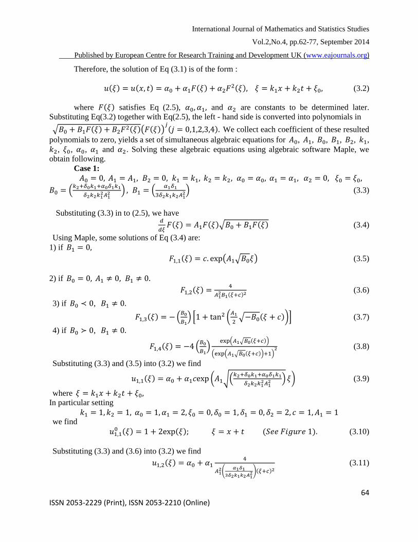
Therefore, the solution of Eq (3.1) is of the form :
𝑢(𝜉) = 𝑢(𝑥, 𝑡) = 𝛼0 + 𝛼1𝐹(𝜉) + 𝛼2𝐹2(𝜉), 𝜉 = 𝑘1𝑥 + 𝑘2𝑡 + 𝜉0, (3.2)
where 𝐹(𝜉) satisfies Eq (2.5), 𝛼0, 𝛼1, and 𝛼2 are constants to be determined later.
Substituting Eq(3.2) together with Eq(2.5), the left - hand side is converted into polynomials in
√𝐵0 + 𝐵1𝐹(𝜉) + 𝐵2𝐹2(𝜉)(𝐹(𝜉))𝑗(𝑗 = 0,1,2,3,4). We collect each coefficient of these resulted
polynomials to zero, yields a set of simultaneous algebraic equations for 𝐴0, 𝐴1, 𝐵0, 𝐵1, 𝐵2, 𝑘1,
𝑘2, 𝜉0, 𝛼0, 𝛼1 and 𝛼2. Solving these algebraic equations using algebraic software Maple, we
obtain following.
Case 1:
𝐴0 = 0, 𝐴1 = 𝐴1, 𝐵2 = 0, 𝑘1 = 𝑘1, 𝑘2 = 𝑘2, 𝛼0 = 𝛼0, 𝛼1 = 𝛼1, 𝛼2 = 0, 𝜉0 = 𝜉0,
𝐵0 = (𝑘2+𝛿0𝑘1+𝛼0𝛿1𝑘1
𝛿2𝑘2𝑘12𝐴1
2 ) , 𝐵1 = (𝛼1𝛿1
3𝛿2𝑘1𝑘2𝐴12) (3.3)
Substituting (3.3) in to (2.5), we have
𝑑
𝑑𝜉𝐹(𝜉) = 𝐴1𝐹(𝜉)√𝐵0 + 𝐵1𝐹(𝜉) (3.4)
Using Maple, some solutions of Eq (3.4) are:
1) if 𝐵1 = 0,
𝐹1,1(𝜉) = 𝑐. exp(𝐴1√𝐵0𝜉) (3.5)
2) if 𝐵0 = 0, 𝐴1 ≠ 0, 𝐵1 ≠ 0.
𝐹1,2(𝜉) =4
𝐴12𝐵1(𝜉+𝑐)2
(3.6)
3) if 𝐵0 ≺ 0, 𝐵1 ≠ 0.
𝐹1,3(𝜉) = −(𝐵0
𝐵1) [1 + tan2 (
𝐴1
2√−𝐵0(𝜉 + 𝑐))] (3.7)
4) if 𝐵0 ≻ 0, 𝐵1 ≠ 0.
𝐹1,4(𝜉) = −4 (𝐵0
𝐵1)
exp(𝐴1√𝐵0(𝜉+𝑐))
(exp(𝐴1√𝐵0(𝜉+𝑐))+1)2 (3.8)
Substituting (3.3) and (3.5) into (3.2) we find
𝑢1,1(𝜉) = 𝛼0 + 𝛼1𝑐exp (𝐴1√(𝑘2+𝛿0𝑘1+𝛼0𝛿1𝑘1
𝛿2𝑘2𝑘12𝐴1
2 ) 𝜉) (3.9)
where 𝜉 = 𝑘1𝑥 + 𝑘2𝑡 + 𝜉0,
In particular setting
𝑘1 = 1, 𝑘2 = 1, 𝛼0 = 1, 𝛼1 = 2, 𝜉0 = 0, 𝛿0 = 1, 𝛿1 = 0, 𝛿2 = 2, 𝑐 = 1, 𝐴1 = 1 we find
𝑢1,10 (𝜉) = 1 + 2exp(𝜉); 𝜉 = 𝑥 + 𝑡 (𝑆𝑒𝑒 𝐹𝑖𝑔𝑢𝑟𝑒 1). (3.10)
Substituting (3.3) and (3.6) into (3.2) we find
𝑢1,2(𝜉) = 𝛼0 + 𝛼14
𝐴12(
𝛼1𝛿1
3𝛿2𝑘1𝑘2𝐴12)(𝜉+𝑐)2
(3.11)

International Journal of Mathematics and Statistics Studies
Vol.2,No.4, pp.62-77, September 2014
Published by European Centre for Research Training and Development UK (www.eajournals.org)
65 ISSN 2053-2229 (Print), ISSN 2053-2210 (Online)
where 𝜉 = 𝑘1𝑥 + 𝑘2𝑡 + 𝜉0,
In particular setting
𝑘1 = 1, 𝑘2 = −2, 𝛼0 = 1, 𝛼1 = 6, 𝜉0 = 0, 𝛿0 = 1, 𝛿1 = 1, 𝛿2 = 1, 𝑐 = 0, 𝐴1 = 1 We find
𝑢1,20 (𝜉) = 1 −
24
𝜉2 ; 𝜉 = 𝑥 − 2𝑡 (𝑆𝑒𝑒 𝐹𝑖𝑔𝑢𝑟𝑒 2). (3.12)
Substituting (3.3) and (3.7) into (3.2) we find
𝑢1,3(𝜉) = 𝛼0 − 3𝛼1 (𝑘2+𝛿0𝑘1+𝛼0𝛿1𝑘1
𝛼1𝛿1𝑘1) [1 + tan2 (
𝐴1
2√−(
𝑘2+𝛿0𝑘1+𝛼0𝛿1𝑘1
𝛿2𝑘2𝑘12𝐴1
2 ) (𝜉 + 𝑐))] (3.13)
where 𝜉 = 𝑘1𝑥 + 𝑘2𝑡 + 𝜉0,
In particular setting
𝑘1 = 1, 𝑘2 = −3, 𝛼0 = 1, 𝛼1 = 3, 𝜉0 = 0, 𝛿0 = 1, 𝛿1 = 1, 𝛿2 = −1
3, 𝑐 = 0, 𝐴1 = 1
We find
𝑢1,30 (𝜉) = 4 + 3tan2 (−
𝜉
2) ; 𝜉 = 𝑥 − 3𝑡 (𝑆𝑒𝑒 𝐹𝑖𝑔𝑢𝑟𝑒 3). (3.14)
Substituting (3.3) and (3.8) into (3.2) we find
𝑢1,4(𝜉) = 𝛼0 − 12𝛼1 (𝑘2+𝛿0𝑘1+𝛼0𝛿1𝑘1
𝛼1𝛿1𝑘1)
exp(𝐴1√(𝑘2+𝛿0𝑘1+𝛼0𝛿1𝑘1
𝛿2𝑘2𝑘12𝐴1
2 )(𝜉+𝑐))
(exp(𝐴1√(𝑘2+𝛿0𝑘1+𝛼0𝛿1𝑘1
𝛿2𝑘2𝑘12𝐴1
2 )(𝜉+𝑐))+1)
2 (3.15)
where 𝜉 = 𝑘1𝑥 + 𝑘2𝑡 + 𝜉0,
In particular setting
𝑘1 = 1, 𝑘2 = 1, 𝛼0 = 1, 𝛼1 = 9, 𝜉0 = 1, 𝛿0 = 1, 𝛿1 = 1, 𝛿2 = 3, 𝑐 = −1, 𝐴1 = 1 We find
𝑢1,40 (𝜉) = 1 −
36exp(𝜉−1)
(exp(𝜉−1)+1)2; 𝜉 = 𝑥 + 𝑡 + 2𝜋 (𝑆𝑒𝑒 𝐹𝑖𝑔𝑢𝑟𝑒 4) (3.16)
Case 2:
𝐴0 = 𝐴0, 𝐴1 = 𝐴1, 𝐵1 = 𝐵1, 𝐵2 = 0, 𝑘1 = 𝑘1, 𝑘2 = 𝑘2, 𝛼0 = 𝛼0, 𝛼2 = 0, 𝜉0 = 𝜉0 (3.17)
𝐵0 = (𝑘2+𝛿0𝑘1+𝛼0𝛿1𝑘1−2𝛿2𝑘2𝑘1
2𝐴0𝐴1𝐵1
𝛿2𝑘2𝑘12𝐴1
2 ), 𝛼1 = (3𝛿2𝑘1𝑘2𝐴1
2𝐵1
𝛿1)
Substituting (3.12) in to (2-5), we have
𝑑
𝑑𝜉𝐹(𝜉) = (𝐴0 + 𝐴1𝐹(𝜉))√𝐵0 + 𝐵1𝐹(𝜉) (3.18)
Using Maple, the solutions of Eq (3.18) are:
1) if 𝐴0 = 0, 𝐵0 = 0, 𝐵1 ≠ 0, 𝐴1 ≠ 0.
𝐹2,1(𝜉) =4
𝐵1𝐴12(𝜉+𝑐)2
(3.19)
2) if 𝐴0 = 0, 𝐵0 ≺ 0, 𝐵1 ≠ 0,

International Journal of Mathematics and Statistics Studies
Vol.2,No.4, pp.62-77, September 2014
Published by European Centre for Research Training and Development UK (www.eajournals.org)
66 ISSN 2053-2229 (Print), ISSN 2053-2210 (Online)
𝐹2,2(𝜉) = −(𝐵0
𝐵1) [1 + tan2 (
𝐴1√−𝐵0
2(𝜉 + 𝑐))] (3.20)
3)𝐴0 = 0, 𝐵0 ≻ 0, 𝐵1 ≠ 0,
𝐹2,3(𝜉) = −4 (𝐵0
𝐵1)
exp(𝐴1√𝐵0)
(exp(𝐴1√𝐵0)+1)2 (3.21)
4) if 𝐵0 = 0, 𝐴1 ≠ 0,𝐴0𝐵1
𝐴1≻ 0,
𝐹2,4(𝜉) =𝐴0
𝐴1tan2 [
𝐴1
2√
𝐴0𝐵1
𝐴1(𝜉 + 𝑐)] (3.22)
5) if 𝐵0 = 0, 𝐴1 ≠ 0,𝐴0𝐵1
𝐴1≺ 0,
𝐹2,5(𝜉) = −(𝐴0
𝐴1) [
exp(𝐴1√−𝐴0𝐵1𝐴1
(𝜉+𝑐))+1
exp(𝐴1√−𝐴0𝐵1𝐴1
(𝜉+𝑐))−1
]
2
(3.23)
6) if𝐴0 = 𝐵0, 𝐴1 = 𝐵1, 𝐴1 ≠ 0,
𝐹2,6(𝜉) = −𝐴0𝐴1
2(𝜉+𝑐)2−4
𝐴13(𝜉+𝑐)2
(3.24)
7)if (𝐴0𝐵1 − 𝐴1𝐵0) = 0, 𝐴1 ≠ 0, 𝐵1 ≠ 0
𝐹2,7(𝜉) = −𝐴1
2𝐵0(𝜉+𝑐)2−4
𝐵1𝐴12(𝜉+𝑐)2
(3.25)
8) if (𝐴0𝐵1−𝐴1𝐵0
𝐴1) = Δ1 ≻ 0, 𝐴1 ≠ 0, 𝐵1 ≠ 0,
𝐹2,8(𝜉) = −(𝐵0
𝐵1) + (
Δ1
𝐵1) tan2 (
𝐴1
2√Δ1(𝜉 + 𝑐)) (3.26)
9) if (𝐴0𝐵1−𝐴1𝐵0
𝐴1) = −Δ1 ≺ 0, 𝐴1 ≠ 0, 𝐵1 ≠ 0,
𝐹2,9(𝜉) = −(𝐴0𝐵1𝐴1
)[exp(𝐴1√Δ1(𝜉+𝑐))−1]2+4𝐵0exp(𝐴1√Δ1(𝜉+𝑐))
𝐵1[exp(𝐴1√Δ1(𝜉+𝑐))+1]2 (3.27)
Substituting (3.17) and (3.19) into (3.2) we find
𝑢2,1(𝜉) = 𝛼0 + (12𝛿2𝑘1𝑘2𝐴1
2𝐵1
𝛿1𝐵1𝐴12 )
1
(𝜉+𝑐)2 (3.28)
where 𝜉 = 𝑘1𝑥 + 𝑘2𝑡 + 𝜉0.
In particular setting
𝑘1 = 1, 𝑘2 = 2, 𝛼0 = −1, 𝜉0 = 0, 𝛿0 = −1, 𝛿1 = 𝛿2 = 1, 𝑐 = 0, 𝐴0 = 0, 𝐴1 = 3, 𝐵1 = 1
we find
𝑢2,10 (𝜉) = −1 +
24
𝜉2 ; 𝜉 = 𝑥 + 2𝑡 (𝑆𝑒𝑒 𝐹𝑖𝑔𝑢𝑟𝑒 5) (3.29)
Substituting (3.17) and (3.20) into (3.2) we find
𝑢2,2(𝜉) = 𝛼0 − (3𝛿2𝑘1𝑘2𝐴1
2𝐵0
𝛿1) [1 + tan2 (
𝐴1√−𝐵0
2(𝜉 + 𝑐))] (3.30)

International Journal of Mathematics and Statistics Studies
Vol.2,No.4, pp.62-77, September 2014
Published by European Centre for Research Training and Development UK (www.eajournals.org)
67 ISSN 2053-2229 (Print), ISSN 2053-2210 (Online)
where 𝜉 = 𝑘1𝑥 + 𝑘2𝑡 + 𝜉0,
In particular setting
𝑘1 = 1, 𝑘2 = 1, 𝛼0 = −3, 𝜉0 = 0, 𝛿0 = 1, 𝛿1 = 𝛿2 = 1, 𝑐 = 0, 𝐴0 = 0, 𝐴1 = 1, 𝐵1 = −1
We find
𝑢2,20 (𝜉) = 3tan2 (
1
2𝜉) ; 𝜉 = 𝑥 + 𝑡 (𝑆𝑒𝑒 𝐹𝑖𝑔𝑢𝑟𝑒 6) (3.31)
Substituting (3.17) and (3.21) into (3.2) we find
𝑢2,3(𝜉) = 𝛼0 − (12𝛿2𝑘1𝑘2𝐴1
2𝐵0
𝛿1)
exp(𝐴1√𝐵0(𝜉+𝑐))
(exp(𝐴1√𝐵0(𝜉+𝑐))+1)2 (3.32)
Where
𝜉 = 𝑘1𝑥 + 𝑘2𝑡 + 𝜉0, In particular setting
𝑘1 = 1, 𝑘2 = 1, 𝛼0 = 1, 𝜉0 = 1, 𝛿0 = 1, 𝛿1 = 1, 𝛿2 = 3, 𝑐 = −1, 𝐴0 = 0, 𝐴1 = 1, 𝐵1 = 2 We find
𝑢2,30 (𝜉) = 1 − 36
exp(𝜉−1)
(exp(𝜉−1)+1)2; 𝜉 = 𝑥 + 𝑡 + 1 (𝑆𝑒𝑒 𝐹𝑖𝑔𝑢𝑟𝑒 7) (3.33)
Substituting (3.17) and (3.22) into (3.2) we find
𝑢2,4(𝜉) = 𝛼0 + (3𝛿2𝑘1𝑘2𝐴0𝐴1𝐵1
𝛿1) tan2 [
𝐴1
2√
𝐴0𝐵1
𝐴1(𝜉 + 𝑐)] (3.34)
where𝜉 = 𝑘1𝑥 + 𝑘2𝑡 + 𝜉0,
In particular setting
𝑘1 = 1, 𝑘2 = 1, 𝛼0 = −1, 𝜉0 = 𝜋, 𝛿0 = 1, 𝛿1 = 1, 𝛿2 =1
2, 𝑐 = 0, 𝐴0 = 1, 𝐴1 = 1, 𝐵1 = 1
We find
𝑢2,40 (𝜉) = −1 +
3
2cot2 (
1
2𝜉) ; 𝜉 = 𝑥 + 𝑡 + 𝜋 (𝑆𝑒𝑒 𝐹𝑖𝑔𝑢𝑟𝑒 8) (3.35)
Substituting (3.17) and (3.23) into (3.2) we find
𝑢2,5(𝜉) = 𝛼0 − (3𝛿2𝑘1𝑘2𝐴0𝐴1𝐵1
𝛿1) [
exp(𝐴1√−𝐴0𝐵1𝐴1
(𝜉+𝑐))+1
exp(𝐴1√−𝐴0𝐵1𝐴1
(𝜉+𝑐))−1
]
2
where 𝜉 = 𝑘1𝑥 + 𝑘2𝑡 + 𝜉0,
In particular setting
𝑘1 = 1, 𝑘2 = 1, 𝛼0 = 2, 𝜉0 = 0, 𝛿0 = 𝛿1 = −1, 𝛿2 = 1, 𝑐 = 0, 𝐴0 = 1, 𝐴1 = −1, 𝐵1 = 1
we find
𝑢2,50 (𝜉) = 2 − 3 (
exp(−𝜉)+1
exp(−𝜉)−1)2
; 𝜉 = 𝑥 + 𝑡 (𝑆𝑒𝑒 𝐹𝑖𝑔𝑢𝑟𝑒 9) (3.36)
Substituting (3.17) and (3.24) into (3.2) we find
𝑢2,6(𝜉) = 𝛼0 − (3𝛿2𝑘1𝑘2𝐵1
𝛿1𝐴1) (
𝐴0𝐴12(𝜉+𝑐)2−4
(𝜉+𝑐)2) (3.37)
where 𝜉 = 𝑘1𝑥 + 𝑘2𝑡 + 𝜉0,
In particular setting
𝑘1 = 1, 𝑘2 = 1, 𝛼0 = 1, 𝜉0 = 0, 𝛿0 = 1, 𝛿1 = 1, 𝛿2 =1
18, 𝑐 = 1, 𝐴0 = 2, 𝐴1 = 3, 𝐵1 = 3

International Journal of Mathematics and Statistics Studies
Vol.2,No.4, pp.62-77, September 2014
Published by European Centre for Research Training and Development UK (www.eajournals.org)
68 ISSN 2053-2229 (Print), ISSN 2053-2210 (Online)
We find
𝑢2,60 (𝜉) = 1 −
18(𝜉+1)2−4
6(𝜉+1)2; 𝜉 = 𝑥 + 𝑡 (𝑆𝑒𝑒 𝐹𝑖𝑔𝑢𝑟𝑒 10) (3.38)
Substituting (3.17) and (3.25) into (3.2) we find
𝑢2,7(𝜉) = 𝛼0 − (3𝛿2𝑘1𝑘2
𝛿1) (
𝐴12𝐵0(𝜉+𝑐)2−4
(𝜉+𝑐)2) (3.39)
Where 𝜉 = 𝑘1𝑥 + 𝑘2𝑡 + 𝜉0,
In particular setting
𝑘1 = 1, 𝑘2 = 1, 𝛼0 = 4, 𝜉0 = 0, 𝛿0 = 1, 𝛿1 = 1, 𝛿2 = 1, 𝑐 = 0, 𝐴0 = 2, 𝐴1 = 1, 𝐵1 = 1
We find
𝑢2,70 (𝜉) = 4 − 6
(𝜉2−2)
𝜉; 𝜉 = 𝑥 + 𝑡 (𝑆𝑒𝑒 𝐹𝑖𝑔𝑢𝑟𝑒 11) (3.40)
Substituting (3.17) and (3.26) into (3.2) we find
𝑢2,8(𝜉) = 𝛼0 + (3𝛿2𝑘1𝑘2𝐵0𝐴1
2
𝛿1) ×
[(−𝐵0
𝐵1) + (
𝐴0𝐵1−𝐴1𝐵0
𝐵1𝐴1) tan2 (
𝐴1
2√(
𝐴0𝐵1−𝐴1𝐵0
𝐴1) (𝜉 + 𝑐))] (3.41)
(46)
Where 𝜉 = 𝑘1𝑥 + 𝑘2𝑡 + 𝜉0,
In particular setting
𝑘1 = 1, 𝑘2 = 1, 𝛼0 = 3, 𝜉0 =𝜋
2, 𝛿0 = 1, 𝛿1 = 1, 𝛿2 = 1, 𝑐 = 0, 𝐴0 = 1, 𝐴1 = 1, 𝐵1 = 2
We find
𝑢2,80 (𝜉) = 3tan2 (
𝜉
2) ; 𝜉 = 𝑥 + 𝑡 +
𝜋
2 (𝑆𝑒𝑒 𝐹𝑖𝑔𝑢𝑟𝑒 12) (3.42)
Substituting (3.17) and (3.27) into (3.2) we find
𝑢2,9(𝜉) = 𝛼0 + (3𝛿2𝑘1𝑘2𝐵1𝐴1
2
𝛿1) [−
(𝐴0𝐵1𝐴1
)[exp(𝐴1√Δ1(𝜉+𝑐))−1]2+4𝐵0exp(𝐴1√Δ1(𝜉+𝑐))
𝐵1[exp(𝐴1√Δ1(𝜉+𝑐))+1]2 ] (3.43)
Where 𝜉 = 𝑘1𝑥 + 𝑘2𝑡 + 𝜉0 ; Δ1 = (𝐴0𝐵1−𝐴1𝐵0
𝐴1)
In particular setting
𝑘1 = 1, 𝑘2 = 1, 𝛼0 = 2, 𝜉0 = 0, 𝛿0 = 1, 𝛿1 = 1, 𝛿2 = 1, 𝑐 = 0, 𝐴0 = 1, 𝐴1 = 1, 𝐵1 = 1
We find
𝑢2,90 (𝜉) = 2 − 3
[(exp(𝜉)−1)2+8exp(𝜉)]
[exp(𝜉)+1]2; 𝜉 = 𝑥 + 𝑡 (𝑆𝑒𝑒 𝐹𝑖𝑔𝑢𝑟𝑒 13) (3.44)
Case3 :
International Journal of Mathematics and Statistics Studies
Vol.2,No.4, pp.62-77, September 2014
Published by European Centre for Research Training and Development UK (www.eajournals.org)
69 ISSN 2053-2229 (Print), ISSN 2053-2210 (Online)
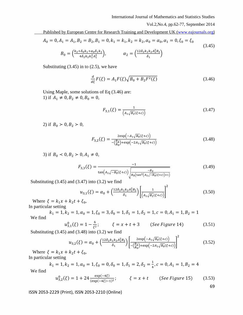
𝐴0 = 0, 𝐴1 = 𝐴1, 𝐵2 = 𝐵2, 𝐵1 = 0, 𝑘1 = 𝑘1, 𝑘2 = 𝑘2, 𝛼0 = 𝛼0, 𝛼1 = 0, 𝜉0 = 𝜉0 (3.45)
𝐵0 = (𝑘2+𝛿0𝑘1+𝛼0𝛿1𝑘1
4𝛿2𝑘2𝑘12𝐴1
2 ), 𝛼2 = (12𝛿2𝑘1𝑘2𝐴1
2𝐵2
𝛿1)
Substituting (3.45) in to (2.5), we have
𝑑
𝑑𝜉𝐹(𝜉) = 𝐴1𝐹(𝜉)√𝐵0 + 𝐵2𝐹2(𝜉) (3.46)
Using Maple, some solutions of Eq (3.46) are:
1) if 𝐴1 ≠ 0, 𝐵2 ≠ 0, 𝐵0 = 0,
𝐹3,1(𝜉) =1
(𝐴1√𝐵2(𝜉+𝑐)) (3.47)
2) if 𝐵0 ≻ 0, 𝐵2 ≻ 0,
𝐹3,2(𝜉) =2exp(−𝐴1√𝐵0(𝜉+𝑐))
−(𝐵2𝐵0
)+exp(−2𝐴1√𝐵0(𝜉+𝑐)) (3.48)
3) if 𝐵0 ≺ 0, 𝐵2 ≻ 0, 𝐴1 ≠ 0,
𝐹3,3(𝜉) =−1
tan(𝐴1√−𝐵0(𝜉+𝑐))√−𝐵2
𝐵0(tan2(𝐴1√−𝐵0(𝜉+𝑐))+1)
(3.49)
Substituting (3.45) and (3.47) into (3.2) we find
𝑢3,1(𝜉) = 𝛼0 + (12𝛿2𝑘1𝑘2𝐴1
2𝐵2
𝛿1) [
1
(𝐴1√𝐵2(𝜉+𝑐))]
2
(3.50)
Where 𝜉 = 𝑘1𝑥 + 𝑘2𝑡 + 𝜉0,
In particular setting
𝑘1 = 1, 𝑘2 = 1, 𝛼0 = 1, 𝜉0 = 3, 𝛿0 = 1, 𝛿1 = 1, 𝛿2 = 1, 𝑐 = 0, 𝐴1 = 1, 𝐵2 = 1 We find
𝑢3,10 (𝜉) = 1 −
6
𝜉2 ; 𝜉 = 𝑥 + 𝑡 + 3 (𝑆𝑒𝑒 𝐹𝑖𝑔𝑢𝑟𝑒 14) (3.51)
Substituting (3.45) and (3.48) into (3.2) we find
𝑢3,2(𝜉) = 𝛼0 + (12𝛿2𝑘1𝑘2𝐴1
2𝐵2
𝛿1) [
2exp(−𝐴1√𝐵0(𝜉+𝑐))
−(𝐵2𝐵0
)+exp(−2𝐴1√𝐵0(𝜉+𝑐))]
2
(3.52)
Where 𝜉 = 𝑘1𝑥 + 𝑘2𝑡 + 𝜉0,
In particular setting
𝑘1 = 1, 𝑘2 = 1, 𝛼0 = 1, 𝜉0 = 0, 𝛿0 = 1, 𝛿1 = 2, 𝛿2 =1
4, 𝑐 = 0, 𝐴1 = 1, 𝐵2 = 4
We find
𝑢3,20 (𝜉) = 1 + 24
exp(−4𝜉)
(exp(−4𝜉)−1)2; 𝜉 = 𝑥 + 𝑡 (𝑆𝑒𝑒 𝐹𝑖𝑔𝑢𝑟𝑒 15) (3.53)
International Journal of Mathematics and Statistics Studies
Vol.2,No.4, pp.62-77, September 2014
Published by European Centre for Research Training and Development UK (www.eajournals.org)
70 ISSN 2053-2229 (Print), ISSN 2053-2210 (Online)
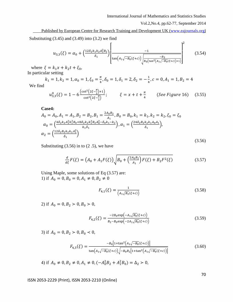
Substituting (3.45) and (3.49) into (3.2) we find
𝑢3,3(𝜉) = 𝛼0 + (12𝛿2𝑘1𝑘2𝐴1
2𝐵2
𝛿1)
[
−1
tan(𝐴1√−𝐵0(𝜉+𝑐))√−𝐵2
𝐵0(tan2(𝐴1√−𝐵0(𝜉+𝑐))+1)] 2
(3.54)
where 𝜉 = 𝑘1𝑥 + 𝑘2𝑡 + 𝜉0,
In particular setting
𝑘1 = 1, 𝑘2 = 1, 𝛼0 = 1, 𝜉0 =𝜋
4, 𝛿0 = 1, 𝛿1 = 2, 𝛿2 = −
1
4, 𝑐 = 0, 𝐴1 = 1, 𝐵2 = 4
We find
𝑢3,30 (𝜉) = 1 − 6
(cot2(2𝜉−𝜋
2)+1)
cot2(2𝜉−𝜋
2)
; 𝜉 = 𝑥 + 𝑡 +𝜋
4 (𝑆𝑒𝑒 𝐹𝑖𝑔𝑢𝑟𝑒 16) (3.55)
Case4:
𝐴0 = 𝐴0, 𝐴1 = 𝐴1, 𝐵2 = 𝐵2, 𝐵1 =2𝐴0𝐵2
𝐴1, 𝐵0 = 𝐵0, 𝑘1 = 𝑘1, 𝑘2 = 𝑘2, 𝜉0 = 𝜉0
𝛼0 = (4𝛿2𝑘2𝐴1
2𝑘12𝐵0+8𝛿2𝑘2𝑘1
2𝐵2𝐴02−𝛿0𝑘1−𝑘2
𝑘1𝛿1) , 𝛼1 = (
24𝛿2𝐵2𝑘2𝑘1𝐴0𝐴1
𝛿1),
𝛼2 = (12𝛿2𝐵2𝑘2𝑘1𝐴1
2
𝛿1)
(3.56)
Substituting (3.56) in to (2 .5), we have
𝑑
𝑑𝜉𝐹(𝜉) = (𝐴0 + 𝐴1𝐹(𝜉))√𝐵0 + (
2𝐴0𝐵2
𝐴1)𝐹(𝜉) + 𝐵2𝐹
2(𝜉) (3.57)
Using Maple, some solutions of Eq (3.57) are:
1) if 𝐴0 = 0, 𝐵0 = 0, 𝐴1 ≠ 0, 𝐵2 ≠ 0
𝐹4,1(𝜉) =1
(𝐴1√𝐵2(𝜉+𝑐)) (3.58)
2) if 𝐴0 = 0, 𝐵2 ≻ 0, 𝐵0 ≻ 0,
𝐹4,2(𝜉) =−2𝐵0exp(−𝐴1√𝐵0(𝜉+𝑐))
𝐵2−𝐵0exp(−2𝐴1√𝐵0(𝜉+𝑐)) (3.59)
3) if 𝐴0 = 0, 𝐵2 ≻ 0, 𝐵0 ≺ 0,
𝐹4,3(𝜉) =−𝐵0[1+tan2(𝐴1√−𝐵0(𝜉+𝑐))]
tan(𝐴1√−𝐵0(𝜉+𝑐))√−𝐵0𝐵2[1+tan2(𝐴1√−𝐵0(𝜉+𝑐))]
(3.60)
4) if 𝐴0 ≠ 0, 𝐵2 ≠ 0, 𝐴1 ≠ 0, (−𝐴02𝐵2 + 𝐴1
2𝐵0) = Δ2 ≻ 0,

International Journal of Mathematics and Statistics Studies
Vol.2,No.4, pp.62-77, September 2014
Published by European Centre for Research Training and Development UK (www.eajournals.org)
71 ISSN 2053-2229 (Print), ISSN 2053-2210 (Online)
𝐹4,4(𝜉) = −2√Δ2exp(−√Δ2(𝜉+𝑐))−𝐴0exp(−2√Δ2(𝜉+𝑐))+𝐴0𝐵2
𝐴1[𝐵2−exp(−2√Δ2(𝜉+𝑐))] (3.61)
5) if 𝐴0 ≠ 0, 𝐵2 ≠ 0, 𝐴1 ≠ 0, (−𝐴02𝐵2 + 𝐴1
2𝐵0) = −Δ2 ≺ 0,
𝐹4,5(𝜉) = −Δ2+Δ2tan2(√Δ2(𝜉+𝑐))+𝐴0tan(√Δ2(𝜉+𝑐))√Δ2𝐵2(1+tan2(√Δ2(𝜉+𝑐)))
𝐴1tan(√Δ2(𝜉+𝑐))√Δ2𝐵2(1+tan2(√Δ2(𝜉+𝑐))) (3.62)
6) if 𝐴0 ≠ 0, 𝐵2 ≠ 0, 𝐴1 ≠ 0, (−𝐴02𝐵2 + 𝐴1
2𝐵0) = 0;
𝐹4,6(𝜉) = [−1
𝐴1√𝐵2(𝜉+𝑐)−
𝐴0
𝐴1] (3.63)
Substituting (3.56) and (3.58) into (3.2) we find
𝑢4,1(𝜉) = (4𝛿2𝑘2𝐴1
2𝑘12𝐵0−𝛿0𝑘1−𝑘2
𝑘1𝛿1) +
(12𝛿2𝐵2𝑘2𝑘1𝐴1
2
𝛿1)
(𝐴1√𝐵2(𝜉+𝑐))2 (3.64)
Where 𝜉 = 𝑘1𝑥 + 𝑘2𝑡 + 𝜉0,
In particular setting
𝑘1 = −1, 𝑘2 = 1, 𝜉0 = −1, 𝛿0 = 2, 𝛿1 = 𝛿2 = 1, 𝑐 = 1, 𝐴1 = 1, 𝐴0 = 0, 𝐵0 = 0, 𝐵2 = 4
We find
𝑢4,10 (𝜉) = −1 −
2
(𝜉+1)2; 𝜉 = −𝑥 + 𝑡 − 1 (𝑆𝑒𝑒 𝐹𝑖𝑔𝑢𝑟𝑒 17) (3.65)
Substituting (3.56) and (3.59) into (3.2) we find
𝑢4,2(𝜉) = (4𝛿2𝑘2𝐴1
2𝑘12𝐵0−𝛿0𝑘1−𝑘2
𝑘1𝛿1) + (
12𝛿2𝐵2𝑘2𝑘1𝐴12
𝛿1) [
−2𝐵0exp(−𝐴1√𝐵0(𝜉+𝑐))
𝐵2−𝐵0exp(−2𝐴1√𝐵0(𝜉+𝑐))]
2
(3.66)
where 𝜉 = 𝑘1𝑥 + 𝑘2𝑡 + 𝜉0,
In particular setting
𝑘1 = 1, 𝑘2 = −1, 𝜉0 = 0, 𝛿0 = 𝛿1 = 𝛿2 = 1, 𝑐 = 0, 𝐴1 = 1, 𝐴0 = 0, 𝐵0 = 4,
𝐵2 = exp(−25)
We find
𝑢4,20 (𝜉) = −16 −
768exp(−25)exp(−4𝜉)
(exp(−25)−4exp(−4𝜉))2 ; 𝜉 = 𝑥 − 𝑡 (𝑆𝑒𝑒 𝐹𝑖𝑔𝑢𝑟𝑒 18) (3.67)
Substituting (3.56) and (3.60) into (3.2) we find
𝑢4,3(𝜉) = (4𝛿2𝑘2𝐴1
2𝑘12𝐵0−𝛿0𝑘1−𝑘2
𝑘1𝛿1) + (
12𝛿2𝐵2𝑘2𝑘1𝐴12
𝛿1)
× (−𝐵0[1+tan2(𝐴1√−𝐵0(𝜉+𝑐))]
tan(𝐴1√−𝐵0(𝜉+𝑐))√−𝐵0𝐵2[1+tan2(𝐴1√−𝐵0(𝜉+𝑐))]
)
2
(3.68)
where 𝜉 = 𝑘1𝑥 + 𝑘2𝑡 + 𝜉0,
In particular setting
International Journal of Mathematics and Statistics Studies
Vol.2,No.4, pp.62-77, September 2014
Published by European Centre for Research Training and Development UK (www.eajournals.org)
72 ISSN 2053-2229 (Print), ISSN 2053-2210 (Online)
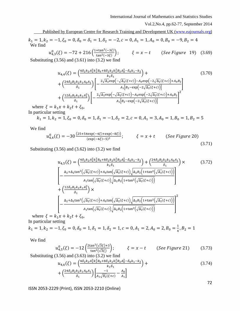
𝑘1 = 1, 𝑘2 = −1, 𝜉0 = 0, 𝛿0 = 𝛿1 = 1, 𝛿2 = −2, 𝑐 = 0, 𝐴1 = 1, 𝐴0 = 0, 𝐵0 = −9, 𝐵2 = 4 We find
𝑢4,30 (𝜉) = −72 + 216 (
1+tan2(−3𝜉)
tan2(−3𝜉)) ; 𝜉 = 𝑥 − 𝑡 (𝑆𝑒𝑒 𝐹𝑖𝑔𝑢𝑟𝑒 19) (3.69)
Substituting (3.56) and (3.61) into (3.2) we find
𝑢4,4(𝜉) = (4𝛿2𝑘2𝐴1
2𝑘12𝐵0+8𝛿2𝑘2𝑘1
2𝐵2𝐴02−𝛿0𝑘1−𝑘2
𝑘1𝛿1) + (3.70)
+(24𝛿2𝐵2𝑘2𝑘1𝐴0𝐴1
𝛿1) [−
2√Δ2exp(−√Δ2(𝜉+𝑐))−𝐴0exp(−2√Δ2(𝜉+𝑐))+𝐴0𝐵2
𝐴1[𝐵2−exp(−2√Δ2(𝜉+𝑐))]]
+(12𝛿2𝐵2𝑘2𝑘1𝐴1
2
𝛿1) [−
2√Δ2exp(−√Δ2(𝜉+𝑐))−𝐴0exp(−2√Δ2(𝜉+𝑐))+𝐴0𝐵2
𝐴1[𝐵2−exp(−2√Δ2(𝜉+𝑐))]]
2
where 𝜉 = 𝑘1𝑥 + 𝑘2𝑡 + 𝜉0,
In particular setting
𝑘1 = 1, 𝑘2 = 1, 𝜉0 = 0, 𝛿0 = 1, 𝛿1 = −1, 𝛿2 = 2, 𝑐 = 0, 𝐴1 = 3, 𝐴0 = 1, 𝐵0 = 1, 𝐵2 = 5
We find
𝑢4,40 (𝜉) = −30
(25+54exp(−4𝜉)+exp(−8𝜉))
(exp(−4𝜉)−5)2; 𝜉 = 𝑥 + 𝑡 (𝑆𝑒𝑒 𝐹𝑖𝑔𝑢𝑟𝑒 20)
(3.71)
Substituting (3.56) and (3.62) into (3.2) we find
𝑢4,5(𝜉) = (4𝛿2𝑘2𝐴1
2𝑘12𝐵0+8𝛿2𝑘2𝑘1
2𝐵2𝐴02−𝛿0𝑘1−𝑘2
𝑘1𝛿1) + (
24𝛿2𝐵2𝑘2𝑘1𝐴0𝐴1
𝛿1) × (3.72)
[−Δ2+Δ2tan2(√Δ2(𝜉+𝑐))+𝐴0tan(√Δ2(𝜉+𝑐))√Δ2𝐵2(1+tan2(√Δ2(𝜉+𝑐)))
𝐴1tan(√Δ2(𝜉+𝑐))√Δ2𝐵2(1+tan2(√Δ2(𝜉+𝑐)))]
+(12𝛿2𝐵2𝑘2𝑘1𝐴1
2
𝛿1) ×
[−Δ2+Δ2tan2(√Δ2(𝜉+𝑐))+𝐴0tan(√Δ2(𝜉+𝑐))√Δ2𝐵2(1+tan2(√Δ2(𝜉+𝑐)))
𝐴1tan(√Δ2(𝜉+𝑐))√Δ2𝐵2(1+tan2(√Δ2(𝜉+𝑐)))]
2
where 𝜉 = 𝑘1𝑥 + 𝑘2𝑡 + 𝜉0,
In particular setting
𝑘1 = 1, 𝑘2 = −1, 𝜉0 = 0, 𝛿0 = 1, 𝛿1 = 1, 𝛿2 = 1, 𝑐 = 0, 𝐴1 = 2, 𝐴0 = 2, 𝐵0 =1
4, 𝐵2 = 1
We find
𝑢4,50 (𝜉) = −12 (
2tan2(√3𝜉)+3
tan2(√3𝜉)) ; 𝜉 = 𝑥 − 𝑡 (𝑆𝑒𝑒 𝐹𝑖𝑔𝑢𝑟𝑒 21) (3.73)
Substituting (3.56) and (3.63) into (3.2) we find
𝑢4,6(𝜉) = (4𝛿2𝑘2𝐴1
2𝑘12𝐵0+8𝛿2𝑘2𝑘1
2𝐵2𝐴02−𝛿0𝑘1−𝑘2
𝑘1𝛿1) + (3.74)
+(24𝛿2𝐵2𝑘2𝑘1𝐴0𝐴1
𝛿1) [
−1
𝐴1√𝐵2(𝜉+𝑐)−
𝐴0
𝐴1]
International Journal of Mathematics and Statistics Studies
Vol.2,No.4, pp.62-77, September 2014
Published by European Centre for Research Training and Development UK (www.eajournals.org)
73 ISSN 2053-2229 (Print), ISSN 2053-2210 (Online)
+(12𝛿2𝐵2𝑘2𝑘1𝐴1
2
𝛿1) [
−1
𝐴1√𝐵2(𝜉+𝑐)−
𝐴0
𝐴1]2
where 𝜉 = 𝑘1𝑥 + 𝑘2𝑡 + 𝜉0,
In particular setting
𝑘1 = 1, 𝑘2 = 1, 𝜉0 = 2, 𝛿0 = 1, 𝛿1 = 1, 𝛿2 = 1, 𝑐 = 3, 𝐴1 = 1, 𝐴0 = 1, 𝐵0 = 1, 𝐵2 = 1
We find
𝑢4,60 (𝜉) = −2
(𝜉2+6𝜉+3)
(𝜉+3)2; 𝜉 = 𝑥 + 𝑡 + 2 (𝑆𝑒𝑒 𝐹𝑖𝑔𝑢𝑟𝑒 22) (3.75)
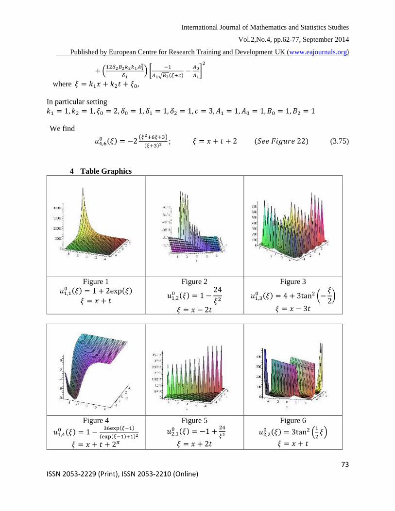
4 Table Graphics
Figure 1
𝑢1,10 (𝜉) = 1 + 2exp(𝜉)
𝜉 = 𝑥 + 𝑡
Figure 2
𝑢1,20 (𝜉) = 1 −
24
𝜉2
𝜉 = 𝑥 − 2𝑡
Figure 3
𝑢1,30 (𝜉) = 4 + 3tan2 (−
𝜉
2)
𝜉 = 𝑥 − 3𝑡
Figure 4
𝑢1,40 (𝜉) = 1 −
36exp(𝜉−1)
(exp(𝜉−1)+1)2
𝜉 = 𝑥 + 𝑡 + 2𝜋
Figure 5
𝑢2,10 (𝜉) = −1 +
24
𝜉2
𝜉 = 𝑥 + 2𝑡
Figure 6
𝑢2,20 (𝜉) = 3tan2 (
1
2𝜉)
𝜉 = 𝑥 + 𝑡

International Journal of Mathematics and Statistics Studies
Vol.2,No.4, pp.62-77, September 2014
Published by European Centre for Research Training and Development UK (www.eajournals.org)
74 ISSN 2053-2229 (Print), ISSN 2053-2210 (Online)
Figure 7
𝑢2,30 (𝜉) =
[1 − 36exp(𝜉−1)
(exp(𝜉−1)+1)2]
𝜉 = 𝑥 + 𝑡 + 1
Figure 8
𝑢2,40 (𝜉) = −1 +
3
2cot2 (
1
2𝜉)
𝜉 = 𝑥 + 𝑡 + 𝜋
Figure 9
𝑢2,50 (𝜉) =
[2 − 3 (exp(−𝜉)+1
exp(−𝜉)−1)2
]
𝜉 = 𝑥 + 𝑡
Figure 10
𝑢2,60 (𝜉) = 1 −
18(𝜉+1)2−4
6(𝜉+1)2
𝜉 = 𝑥 + 𝑡
Figure 11
𝑢2,70 (𝜉) = 4 − 6
(𝜉2−2)
𝜉
𝜉 = 𝑥 + 𝑡
Figure 12
𝑢2,80 (𝜉) = 3tan2 (
𝜉
2)
𝜉 = 𝑥 + 𝑡 +𝜋
2
International Journal of Mathematics and Statistics Studies
Vol.2,No.4, pp.62-77, September 2014
Published by European Centre for Research Training and Development UK (www.eajournals.org)
75 ISSN 2053-2229 (Print), ISSN 2053-2210 (Online)
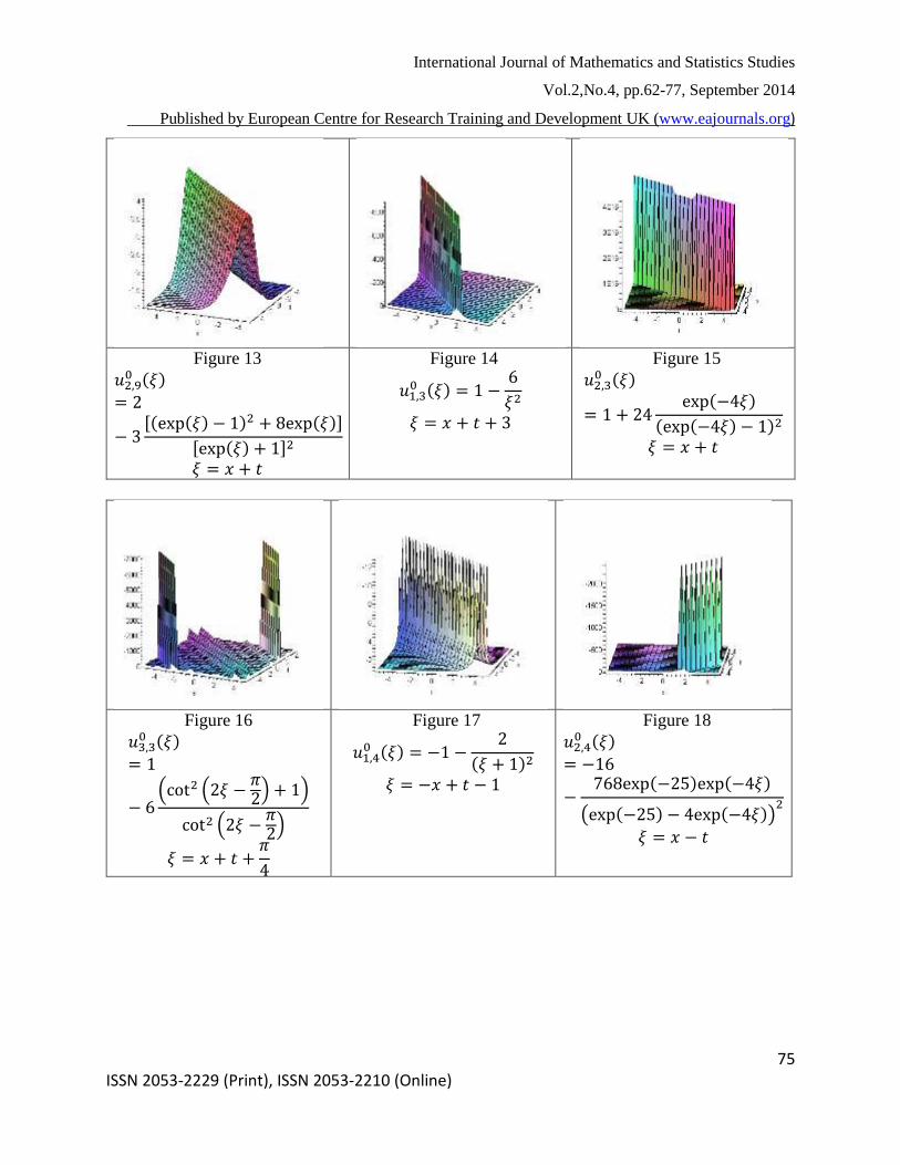
Figure 13
𝑢2,90 (𝜉)
= 2
− 3[(exp(𝜉) − 1)2 + 8exp(𝜉)]
[exp(𝜉) + 1]2
𝜉 = 𝑥 + 𝑡
Figure 14
𝑢1,30 (𝜉) = 1 −
6
𝜉2
𝜉 = 𝑥 + 𝑡 + 3
Figure 15
𝑢2,30 (𝜉)
= 1 + 24exp(−4𝜉)
(exp(−4𝜉) − 1)2
𝜉 = 𝑥 + 𝑡
Figure 16
𝑢3,30 (𝜉)
= 1
− 6(cot2 (2𝜉 −
𝜋2) + 1)
cot2 (2𝜉 −𝜋2)
𝜉 = 𝑥 + 𝑡 +𝜋
4
Figure 17
𝑢1,40 (𝜉) = −1 −
2
(𝜉 + 1)2
𝜉 = −𝑥 + 𝑡 − 1
Figure 18
𝑢2,40 (𝜉)
= −16
−768exp(−25)exp(−4𝜉)
(exp(−25) − 4exp(−4𝜉))2
𝜉 = 𝑥 − 𝑡

International Journal of Mathematics and Statistics Studies
Vol.2,No.4, pp.62-77, September 2014
Published by European Centre for Research Training and Development UK (www.eajournals.org)
76 ISSN 2053-2229 (Print), ISSN 2053-2210 (Online)
Figure 19
𝑢3,40 (𝜉) = −72 +
216 (1+tan2(−3𝜉)
tan2(−3𝜉))
𝜉 = 𝑥 − 𝑡
Figure 20
𝑢4,40 (𝜉) =
−30(25+54exp(−4𝜉)+exp(−8𝜉))
(exp(−4𝜉)−5)2
𝜉 = 𝑥 + 𝑡
Figure 21
𝑢5,40 (𝜉) =
−12 (2tan2(√3𝜉)+3
tan2(√3𝜉))
𝜉 = 𝑥 − 𝑡
Figure 22
𝑢6,40 (𝜉) = −2
(𝜉2+6𝜉+3)
(𝜉+3)2
𝜉 = 𝑥 + 𝑡 + 2
CONCLUSION
In this article, we have proposed a new method called calibrating auxiliary differential equation
method using the generalized wave transformation (2.2), to obtain the exact solutions for BBM equation. The main advantage of this method is its capability of greatly reducing the size of

International Journal of Mathematics and Statistics Studies
Vol.2,No.4, pp.62-77, September 2014
Published by European Centre for Research Training and Development UK (www.eajournals.org)
77 ISSN 2053-2229 (Print), ISSN 2053-2210 (Online)
computational work compared to existing techniques.
The method could be used for a large class of very interesting nonlinear equations.
REFERENCES [1] E. Fan (2000). Darboux transformation and soliton - like solutions for the Gerdjikov-Ivanov equation, J phys A,
33 , 6925-33.
[2] J. B. Liu, K. Q. Yang (2004). The extended F-expansion method and exact solutions of nonlinear PDEs, Chaos
Solitions Fractals, 22 ,111-121.
[3] J. H. He, M. A. Abdou (2007).New periodic solutions for nonlinear evolution equations using Exp-function
method, Chaos, Solitons Fractals , 34, 1421-1429.
[4] E. J. Parkes, B. R. Duffy (1969). An automated tanh-function method for findind solitary wave solutions to
nonlinear evolution equations, Comp. Phys. Commun, 98 , 288-300.
[5] S. D. Zhu (2007). Exact solutions for the high-order dispersive cubic-quintic nonlinear Schrodinger equation by
the extended hyperbolic auxiliary equation method, Chaos Solitons Fract, 34, 1608-1612.
[6] Mohammad Ali Bashir and Lama Abdulaziz Alhakim (2013). New F expansion method and its application to
modified Kdv equation , Vol. 5, no. 4, 83-94.
[7] Mohammad Ali Bashir and Alaaeddin Amin Moussa (2014). New approach of (𝐺 ′
𝐺) expansion method.
Applications to Kdv equation , Vol. 6, no. 1, 24-32.
[8] A. M. Wazawaz (2006).New traveling wave solutions of differential physical structures to generalized BBM
equation, Phys. Lett. A., 355, 358-362.
[9] Marwan T. Alquran (2012).Solitons and Periodic Solutions to Nonlinear Partial Differential Equations by the
Sine-Cosine Method, Appl. Math. Inf. Sci, 6, No. 1, 85-88
[10] Zayed E. M. E., Zedan H. A. and Geprell K. A (2004). Group analysis and modified tanh-function to find the
invariant solutions and soliton solution for nonlinear Euler equations, Int J Non Sci and Nume Simul, 21, 221-
234.
[11] He J. H. and Wu X. H (2006). Exp-function method for nonlinear wave equations, Chaos, Solitons and Fractals
, 30, 700-708.
[12] Yong Chen and Qi Wang (2005). Extended Jacobi elliptic function rational expansion method and abundant
families of Jacobi elliptic function solutions to (1+1)-dimensional dispersive long wave equation, Chaos,
Solitons and Fractals , 24, 745-757.
[13] S. ZHANG (2007) A generalized new auxiliary equation method and its application to the (2+1)- dimensional
breaking soliton equations, Appl. Math. Comput , 190, 510-516.
[14] E. YOMBA (2008). A generalized auxiliary equation method and its application to nonlinear Klein- Gordon
and generalized nonlinear Camassa-Holm equations, Phys. Lett. A. , 372, 1048 - 1060.
[15] F. KANGALGIL AND F. AYAZ (2008). New exact traveling wave solutions for the Ostrovsky equation, Pyys.
Lett. A. , 372, 1831-1835.