c. maes, f. redig and e. saada- abelian sandpile models in infinite volume

8/3/2019 C. Maes, F. Redig and E. Saada- Abelian Sandpile Models in Infinite Volume

http://slidepdf.com/reader/full/c-maes-f-redig-and-e-saada-abelian-sandpile-models-in-infinite-volume 1/21

Abelian Sandpile Models in Infinite Volume∗

C. Maes †

F. Redig ‡

E. Saada §

30th May 2004

Abstract: Since its introduction by Bak,Tang and Wiesenfeld, the abelian sandpiledynamics has been studied extensively in finite volume. There are many problems posedby the existence of a sandpile dynamics in an infinite volume S : its invariant distributionshould be the thermodynamic limit (does the latter exist?) of the invariant measure forthe finite volume dynamics; the extension of the sand grains addition operator to infinitevolume is related to the boundary effects of the dynamics in finite volume; finally, thecrucial difficulty of the definition of a Markov process in infinite volume is that, due tosand avalanches, the interaction is long range, so that no use of the Hille-Yosida theoremis possible. In that review paper, we recall the needed results in finite volume, thenexplain how to deal with infinite volume when S = Z, S = T is an infinite tree, S = Zd

with d large, and when the dynamics is dissipative (i.e. sand grains may disappear ateach toppling) 1.

1 Introduction

Since their appearance in [2], sandpile models have been studied intensively. One phys-ical motivation is the phenomenon of ‘self-organized criticality’. The steady state typ-ically exhibits power law decay of correlations and of avalanche sizes with universalcritical exponents found in many computer simulations and in a wide range of naturalphenomena, such as forest fires, earthquakes, etc.(see e.g. [18] for an overview of variousmodels).

∗

†Instituut voor Theoretische Fysica, K.U.Leuven, Celestijnenlaan 200D, 3001 Leuven, Belgium‡Faculteit Wiskunde en Informatica, Technische Universiteit Eindhoven, Postbus 513, 5600 MB

Eindhoven, The Netherlands§

CNRS, UMR 6085, Laboratoire de mathematiques Raphael Salem, Universite de Rouen, site Col-bert, 76821 Mont-Saint-Aignan Cedex, France1MSC 2000: Primary-82C22; secondary-60K35.

Key-words: Sandpile dynamics, Nonlocal interactions, Interacting particle systems, Thermodynamiclimit.

1



The abelian sandpile model in a finite volume V describes the evolution on a latticeof configurations η of discrete height-variables , which can be thought as local slopes of asandpile. Sand grains are randomly added on the sites x ∈ V , and if at a site the heightvalue for configuration η exceeds some critical value γ , then that ‘unstable’ site ‘topples’,i.e., gives an equal portion of its grains to each of its neighboring sites which in turn canbecome unstable and topple etc., until every site has again a subcritical height-value.An unstable site thus creates an ‘avalanche’ involving possibly the toppling of manysites around it. The range of this avalanche depends on the configuration, making the

dynamics highly non-local. The action of the ‘addition operator’ ax,V consists in theinstantaneous passage from configuration η to which a sand grain has been added onsite x to the stable configuration ax,V η reached after the avalanche has ended.

This model has a rich mathematical structure, first discovered by Dhar (see forinstance [4, 5, 9, 17, 15]). The main tool in its analysis is the ‘abelian group’ of additionoperators, identified with the set RV of recurrent configurations for the dynamics. Thestationary measure for the dynamics is the uniform measure μV on RV .

We aim at defining the model on infinite graphs S , or better, to understand howthe process settles down in a stationary regime as the volume increases. The mainproblems to overcome are the non-locality and the dependence to boundary-conditionsof the dynamics.

The questions we are interested in are, in successive order:

Q1. The convergence of the measures μV when V ↑ S to a probability measure μ.

Q2. The extension of the addition operators ax,V to operators ax on S ; the abelianproperty for those ax; the invariance of μ under those ax.

Q3. The construction of a Markov process that extends the sandpile dynamics fromfinite to infinite volume, corresponding to Poissonian addition of sand grains in infinitevolume; the invariance and ergodicity of μ for this process.

These questions have been partially or completely answered for the one-dimensionallattice S = Z, for infinite homogeneous trees, for S = Z

d with d large, and for dissipative

models, in the papers [12, 13, 14, 1, 10]. In this review, we explain the main content of these papers.

In Section 2, we recall the definition and properties of the model in a finite volumeV , with details on the tools we need later on. We then explain our methods to deal withthe above questions, and their applications to the different settings of S : we considersuccessively Q1 in Section 4, Q2 in Section 5, Q3 in Section 6.

We will analyse separately the dynamics on S = Z, in Section 3: as we will noticefrom examples of Section 2, it is possible there to guess an explicit and simple expres-sion of axη, so that our construction is specific, and uses monotonicity. The invariantmeasure for the dynamics will be the Dirac measure concentrating on the ‘full config-

uration’ (i.e. the height is the critical value on each site). This result seems intuitive:since we continue adding sand at each lattice site, after some time every site will havereceived enough extra sand particles, and once the configuration is full, it remains full.Nevertheless, this intuitive picture is somewhat dangerous, since we are working ininfinite volume, and sand particles could possibly ‘disappear’ at infinity. Indeed, the

2



same statement is not true anymore in the other cases, where the measure μ will notbe trivial.

Our tools come from the theory of interacting particle systems (see [11]). However,due to the non-locality of the dynamics, no use of the usual techniques, such as theHille-Yosida theorem, is possible. Indeed, the Markov processes we will construct ininfinite volume turn out not to be Feller. In the cases we study, we will take advantageof the existing results for the dynamics in finite volume: for the infinite tree, we relyon the very precise results derived in [6]. For dissipative models, the critical value γ is

larger than the maximal number of neighbors of a site in S , and at the toppling of aconsiderable fraction of sites, grains disappear in a sink associated to the volume. Moreprecisely, in terms of the simple random walk on S with a sink associated to the volume,the Green’s function decays exponentially in the lattice distance. There is a strongercontrol of the non-locality, which induces that ‘avalanche clusters’ are almost surelyfinite. For Zd with d large, one uses Priezzhev’s ideas on waves ([9]), and properties of two-component spanning trees.

2 Finite volume model

This section contains definitions and properties of abelian sandpiles in finite volumethat we need later on. In [4], [5], [9], [17] and [15], the reader will find more details.

The infinite graphs S on which is constructed the abelian sandpile dynamics areS = Z

d, infinite trees S = T, and ‘strips’, that is, S = Z × {1, . . . , }, for some integer > 1 (notice that = 1 corresponds to S = Z

d with d = 1). Finite subsets of S will bedenoted by V, W ; we write S = {W ⊂ S : W finite}. We denote by ∂ eV - resp. ∂ iV - theexternal - resp. internal - boundary of V , i.e. all the sites in S \ V - resp. V - that havea nearest neighbor in V - resp. in S \ V . Let N be the maximal number of neighbors of a site in S , e.g., N = 2d for S = Z

d and N = 4 for S = Z× {1, . . . , }, ≥ 3. The statespace of the process in infinite volume is Ω = {1, . . . , γ }S , for some integer γ ≥ N .

We fix V ∈ S , a nearest neighbor connected subset of S . Then ΩV = {1, . . . , γ }V isthe state space of the process in the finite volume V . We denote by N V (x) the numberof nearest neighbors of x in V .

A (infinite volume) height configuration η is a mapping from S to N = {1, 2,...}assigning to each site x a ‘number of sand grains’ η(x) ≥ 1. If η ∈ Ω, it is called astable configuration. Otherwise η is unstable . For η ∈ Ω, ηV is its restriction to V ,and for η, ζ ∈ Ω, ηV ζ V c denotes the configuration whose restriction to V (resp. V c)coincides with ηV (resp. ζ V c).

The configuration space Ω is endowed with the product topology, making it intoa compact metric space. A function f : Ω → R is local if there is W ∈ S such that

ηW = ζ W implies f (η) = f (ζ ). The minimal (in the sense of set ordering) such W isthe dependence set Df of f . A local function can be seen as a function on ΩW for allW ⊃ Df , and every function on ΩW can be seen as a local function on Ω. The set L of all local functions is uniformly dense in the set C(Ω) of all continuous functions on Ω.

3



2.1 The dynamics in finite volume

The toppling matrix Δ on S is defined by, for x, y ∈ S ,

Δxx = γ,

Δxy = −1 if x and y are nearest neighbors,

Δxy = 0 otherwise (2.1)

We denote by ΔV the restriction of Δ to V × V (remark that for x ∈ V , ΔV xx = Δxx).

A site x ∈ V is dissipative in the volume V if y∈V

Δxy > 0. (2.2)

Thus if γ > N , every site is dissipative. If γ = N , the sites of ∂ iV are the onlydissipative sites in V .

Examples 2.3 1. For S = Zd, we have γ = N = 2d.

2. For the binary tree, γ = N = 3.

3. For the strip S = Z× {1, . . . , }, γ = 4, and N = 3 for = 2, N = 4 for > 2.

4. For dissipative systems on S = Zd with d ≥ 2, we have N = 2d, γ > N .

To define the sandpile dynamics in the volume V , we first introduce the toppling of a site x ∈ V as the mapping T x : NV → N

V defined by

T x(η)(y) = η(y) − ΔV xy if η(x) > Δxx,

= η(y) otherwise. (2.4)

In words, site x topples if and only if its height is strictly larger than γ , by transferring−ΔV

xy ∈ {0, 1} grains to site y = x and losing itself in total γ grains. Notice that if x isa dissipative site, then, upon toppling, some grains are lost.Toppling rules commute on unstable configurations, that is, for x, y ∈ V such thatη(x) > γ = Δxx and η(y) > γ = Δyy :

T x (T y(η)) = T y (T x(η)) (2.5)

The toppling transformation is the mapping T : NV → ΩV defined by the requirementthat for η ∈ N

V , T (η) arises from η by toppling , i.e. there exists a k-tuple (x1, . . . , xk)of sites in V such that T (η) = (k

i=1 T xi)(η). The existence of dissipative sites implies

that stabilization of an unstable configuration is always possible. The fact that T iswell-defined , that is, that the same final stable configuration is obtained irrespective of the order of the topplings, is a consequence of the commutation property (see [15] fora complete proof).

4



For x ∈ V , η ∈ NV , we denote by ex (resp. eV

x ) the mapping from S (resp. V ) to{0, 1} which is one at site x and zero at all other sites, and by η + eV

x the configurationobtained from η by adding one grain to site x. The addition operator defined by

ax,V : ΩV → ΩV ; η → ax,V η = T (η + eV x ) (2.6)

represents the effect of adding a grain to the stable configuration η and letting a stableconfiguration arise by toppling. Because T is well-defined, and because of (2.5), thecomposition of addition operators is commutative. This is the so-called abelian property

of the model, which is a crucial simplification in its mathematical analysis.We can now define a discrete time Markov chain {ηn : n ≥ 0} on ΩV by picking a

point x ∈ V randomly at each discrete time step and applying the addition operatorax,V to the configuration. We define also a continuous time Markov process {ηt : t ≥ 0}with infinitesimal generator

L0,ϕV f (η) =

x∈V

ϕ(x)[f (ax,V η) − f (η)]; (2.7)

this is a pure jump process on ΩV , where ϕ : S → (0, ∞) is the addition rate function.

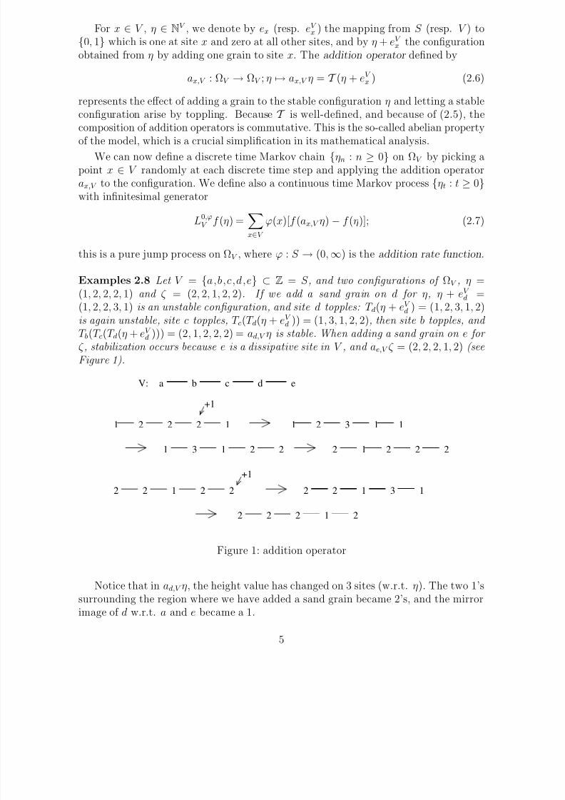
Examples 2.8 Let V = {a,b,c,d,e} ⊂ Z = S , and two configurations of ΩV , η =(1, 2, 2, 2, 1) and ζ = (2, 2, 1, 2, 2). If we add a sand grain on d for η, η + eV

d =(1, 2, 2, 3, 1) is an unstable configuration, and site d topples: T d(η + eV

d ) = (1, 2, 3, 1, 2)is again unstable, site c topples, T c(T d(η + eV

d )) = (1, 3, 1, 2, 2), then site b topples, and T b(T c(T d(η + eV

d ))) = (2, 1, 2, 2, 2) = ad,V η is stable. When adding a sand grain on e for ζ , stabilization occurs because e is a dissipative site in V , and ae,V ζ = (2, 2, 2, 1, 2) (seeFigure 1).

2 2 2 1 2

2 2 2 11

+1

1 2 3 1 1

1 3 1 2 2 22 1 2 2

+1

2 2 1 2 12 2 1 3

a b c d eV:

2

Figure 1: addition operator

Notice that in ad,V η, the height value has changed on 3 sites (w.r.t. η). The two 1’ssurrounding the region where we have added a sand grain became 2’s, and the mirrorimage of d w.r.t. a and e became a 1.

5



2.2 Recurrent configurations, invariant measure

We call RV the set of recurrent configurations for {ηn : n ≥ 0} (or for its continuoustime version {ηt}) , i.e. those for which P η(ηn = η infinitely often) = 1, where P ηdenotes the distribution of {ηn : n ≥ 0} starting from η0 = η ∈ ΩV .

Proposition 2.9 1. RV contains only one recurrent class.

2. The addition operators ax,V generate an abelian group G of permutations of RV .

That group acts transitively on RV , in particular |G| = |RV | = det(ΔV ).

3. The uniform measure on recurrent configurations

μV =

η∈RV

1

|RV |δη (2.10)

is invariant under the action of ax,V and of a−1x,V , x ∈ V ( δη is the Dirac measureon configuration η).

For the proof of this proposition, we refer to [4, 13, 15]. We emphasize that adding

Δx,x particles at a site x ∈ V makes the site topple, and −ΔV x,y particles are trans-

ferred to y. This gives aΔx,x

x,V =y=x

a−ΔV

x,y

y,V , that we rewrite as a closure relation that

characterizes the group G: y∈V

aΔV xy

y,V = Id (2.11)

2.3 Burning algorithm and consequences

2.3.1 Burning algorithm

A configuration η ∈ ΩV belongs to RV if it passes the burning algorithm (see [4]), whichis described as follows. Pick η ∈ ΩV and erase the set V 1 of all sites x ∈ V with a heightstrictly larger than the number of neighbors of that site in V :

η(x) > N V (x) (2.12)

Iterate this procedure for the new volume V \ V 1, and so on. If at the end some non-empty subset V f is left, then η satisfies, for all x ∈ V f ,

η(x) ≤ N V f (x)

and the restriction ηV f is called a forbidden subconfiguration (fsc). If η does not con-tain any fsc, the configuration is called allowed. The set AV of allowed configurationscoincides with the set of recurrent configurations, AV = RV (see [9], [15], [17]).

6



1

1 12 1 1 2

2 2 1 2 2 1

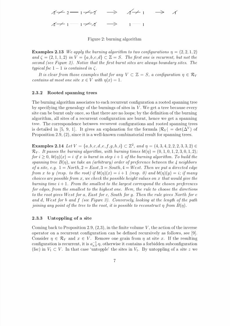
Figure 2: burning algorithm

Examples 2.13 We apply the burning algorithm to two configurations η = (2, 2, 1, 2)

and ζ = (2, 1, 1, 2) in V = {a,b,c,d} ⊂ Z = S . The first one is recurrent, but not thesecond (see Figure 2). Notice that the first burnt sites are always boundary sites. Thetypical fsc 1 − 1 is contained in ζ .

It is clear from those examples that for any V ⊂ Z = S , a configuration η ∈ RV

contains at most one site x ∈ V with η(x) = 1.

2.3.2 Rooted spanning trees

The burning algorithm associates to each recurrent configuration a rooted spanning treeby specifying the genealogy of the burnings of sites in V . We get a tree because every

site can be burnt only once, so that there are no loops; by the definition of the burningalgorithm, all sites of a recurrent configuration are burnt, hence we get a spanningtree. The correspondence between recurrent configurations and rooted spanning treesis detailed in [5, 9, 1]. It gives an explanation for the formula |RV | = det(ΔV ) of Proposition 2.9, (2), since it is a well-known combinatorial result for spanning trees.

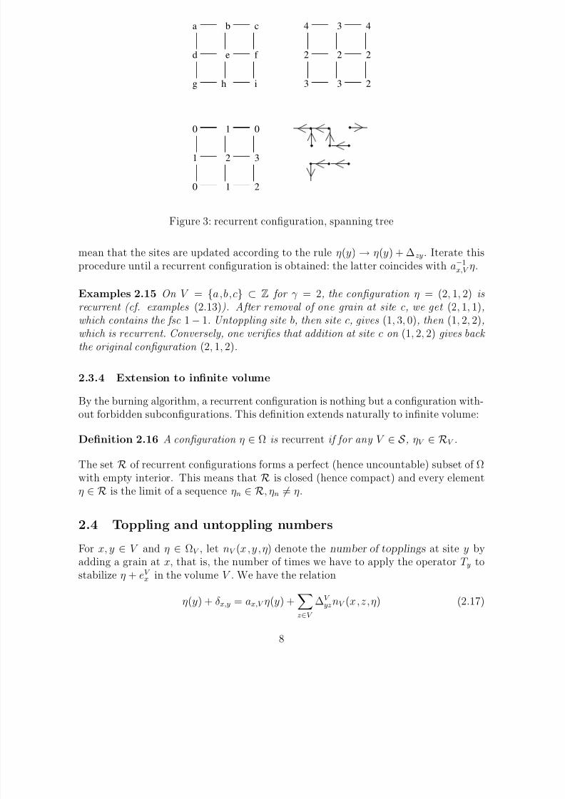
Examples 2.14 Let V = {a,b,c,d,e,f,g,h,i} ⊂ Z2, and η = (4, 3, 4, 2, 2, 2, 3, 3, 2) ∈

RV . It passes the burning algorithm, with burning times bt(η) = (0, 1, 0, 1, 2, 3, 0, 1, 2); for i ≥ 0, bt(η)(x) = i if x is burnt in step i + 1 of the burning algorithm. To build thespanning tree B(η), we take an (arbitrary) order of preference between the 4 neighborsof a site, e.g. 1 = North, 2 = East, 3 = South, 4 = West. Then we put a directed edge

from x to y (resp. to the root) if bt(η)(x) = i + 1 (resp. 0) and bt(η)(y) = i; if many choices are possible from x, we check the possible height values on x that would give theburning time i + 1. From the smallest to the largest correspond the chosen preferences

for edges, from the smallest to the highest one. Here, the rule to choose the directionsto the root gives West for a, East for c, South for g. Then the rule gives North for eand d, West for b and f (see Figure 3). Conversely, looking at the length of the path

joining any point of the tree to the root, it is possible to reconstruct η from B(η).

2.3.3 Untoppling of a site

Coming back to Proposition 2.9, (2,3), in the finite volume V , the action of the inverseoperator on a recurrent configuration can be defined recursively as follows, see [9].Consider η ∈ RV and x ∈ V . Remove one grain from η at site x. If the resultingconfiguration is recurrent, it is a−1x,V η, otherwise it contains a forbidden subconfiguration(fsc) in V 1 ⊂ V . In that case ‘untopple’ the sites in V 1. By untoppling of a site z we

7



a b c

d e f

g ih

4 3 4

2 2 2

3 3 2

0 1 0

1 2 3

0 1 2

Figure 3: recurrent configuration, spanning tree

mean that the sites are updated according to the rule η(y) → η(y) + Δzy . Iterate thisprocedure until a recurrent configuration is obtained: the latter coincides with a−1x,V η.

Examples 2.15 On V = {a,b,c} ⊂ Z for γ = 2, the configuration η = (2, 1, 2) isrecurrent (cf. examples (2.13)). After removal of one grain at site c, we get (2, 1, 1),which contains the fsc 1 − 1. Untoppling site b, then site c, gives (1, 3, 0), then (1, 2, 2),which is recurrent. Conversely, one verifies that addition at site c on (1, 2, 2) gives back the original configuration (2, 1, 2).

2.3.4 Extension to infinite volume

By the burning algorithm, a recurrent configuration is nothing but a configuration with-

out forbidden subconfigurations. This definition extends naturally to infinite volume:

Definition 2.16 A configuration η ∈ Ω is recurrent if for any V ∈ S , ηV ∈ RV .

The set R of recurrent configurations forms a perfect (hence uncountable) subset of Ωwith empty interior. This means that R is closed (hence compact) and every elementη ∈ R is the limit of a sequence ηn ∈ R, ηn = η.

2.4 Toppling and untoppling numbers

For x, y ∈ V and η ∈ ΩV , let nV (x,y,η) denote the number of topplings at site y by

adding a grain at x, that is, the number of times we have to apply the operator T y tostabilize η + eV

x in the volume V . We have the relation

η(y) + δx,y = ax,V η(y) +z∈V

ΔV yz nV (x,z,η) (2.17)

8



Defining

GV (x, y) =

μV (dη) nV (x,y,η) (2.18)

one obtains, by integrating (2.17) over μV :

GV (x, y) = (ΔV )−1xy . (2.19)

The Markov inequality and (2.18) provide an estimate of the probability that site ytopples after addition at site x:

μV ( nV (x,y,η) ≥ 1) ≤ GV (x, y) (2.20)

This inequality plays a crucial role in controlling avalanches when the volume increases.

Call n−V (x,y,η) the number of untopplings at site y by removing one grain from xand from untoppling sites until a recurrent configuration is obtained. As previously,

n−V (x,y,η)μV (dη) = GV (x, y) (2.21)

3 A sandpile dynamics on Z

In this section we summarize our construction of the infinite volume sandpile dynamicson the one-dimensional lattice Z. We refer to [12] for details.

3.1 Addition operator.

We use the simple and explicit form of the evolution in finite volume (that we explainedin examples 2.8) to define a toppling transformation directly on Z. For any configurationη ∈ Ω = {1, 2}Z and any lattice site i ∈ Z, we define (with the convention inf ∅ := +∞)

k+(i, η) := inf { j ≥ 0 : η(i + j) = 1}, (3.1)

the distance from i to the first site to its right (including i) with value 1 and

k−(i, η) := inf { j > 0 : η(i − j) = 1}, (3.2)

the positive distance from i to the first site with value 1 to its left. We distinguish fivecases to define aiη = T (η + ei) (cf. (2.6)):

1. k+(i, η) = 0, i.e. η(i) = 1, then aiη = η + ei.

2. k+(i, η) > 0, k+(i, η) ∨ k−(i, η) < ∞, then

aiη = η + ei+k+(i,η) + ei−k−(i,η) − ei+k+(i,η)−k−(i,η) (3.3)

3. k+(i, η) = ∞, k−(i, η) < ∞, then aiη = η + ei−k−(i,η).

9



4. k+(i, η) < ∞, k−(i, η) = ∞, then aiη = η + ei+k+(i,η).

5. k+(i, η) = k−(i, η) = ∞ (i.e. η ≡ 2), then aiη = η.

As in examples 2.8, case 2 says that when we add a sand grain on a site i with height 2surrounded by two sites i + k+(i, η), i − k−(i, η) with height 1, those two 1’s become 2’s,and the mirror image i + k+(i, η) − k−(i, η) of i w.r.t. the sites i + k+(i, η), i − k−(i, η)becomes a 1. Cases 3,4,5 are conventions to define aiη for all η ∈ Ω, and to write downa formal generator. However, these choices are ‘correct’, as will follow from Theorem

3.12.Note that the transformations ai and a j commute, i.e.

ai(a j (η)) = a j (ai(η)), ∀i, j ∈ Z, ∀η ∈ Ω. (3.4)

3.2 Construction of the sandpile process.

In the construction of the sandpile process in dimension 1, monotonicity plays a crucialrole. We recall its definition and main properties, and refer to [11], Chapter 2, Section2 for details.

For η, ξ ∈ Ω, η ≤ ξ if η(x) ≤ ξ(x) for all x ∈ Z. A function f : Ω → R is monotoneif η ≤ ξ implies f (η) ≤ f (ξ), for all η, ξ ∈ Ω. We denote by M the class of all monotonebounded Borel measurable functions. A Markov process {ηt : t ≥ 0} on Ω with Markovsemigroup {S (t) : t ≥ 0} is monotone if f ∈ M implies S (t)f ∈ M. Two probabilitymeasures μ and ν satisfy μ ≤ ν if for all monotone functions,

f dμ ≤

f dν .

A usual way to prove monotonicity of a Markov process is by explicitly constructinga coupling of path space measures such that for η ≤ ξ one has P η,ξ (ηt ≤ ξt, ∀t ≥ 0) = 1.

Let Ωf be the set of configurations η with a finite number A(η) of critical sites, i.e.

Ωf := {η ∈ Ω : η−1({2}) = A(η) ∈ S}. (3.5)

The correspondence between S and Ωf via A → ηA, where η−1A ({2}) = A (or η → A(η))is one-to-one.

The following formal generator is well-defined for every local function f for η ∈ Ωf

Lf (η) = Lbf (η) + Laf (η), (3.6)

where the “birth part”

Lbf (η) =i∈Z

χ(η(i) = 1)[f (η + ei) − f (η)] (3.7)

corresponds to a pure birth process, thus is a well-defined generator of a Feller semi-group. The “avalanche part”

Laf (η) =i∈Z

χ(η(i) = 2)[f (aiη) − f (η)] (3.8)

10



however gives technical problems related to the nonlocality of the transformation ai.One cannot run the standard Hille-Yoshida program, which would give a Feller semi-group associated to Lb + La.

We proceed in three steps to construct the sandpile process:

1. Definition of a process associated to La on Ωf . Construction of a non-trivialcoupling showing that this process is monotone.

2. Definition of a process associated to La + births in the finite interval [−n, n] on

Ωf . Construction of a coupling showing that this process is still monotone. Thisgives us a semigroup defined on f ∈ M by S n(t)f (η) = limη∈Ωf , η↑η S n(t)f (η),where limη↑η denotes the limit along sequences {ηn, n ∈ N} ⊂ Ωf such thatηn ≤ ηn+1.

3. Monotonicity of the semigroups S n(t) in n, i.e., for all f ∈ M, η ∈ Ω, t ≥0, S n+1(t)f (η) ≥ S n(t)f (η).

We finally define the sandpile process as the process associated to the semigroup

S (t)f (η) = limn↑∞

limη∈Ωf ,η↑η

S n(t)f (η). (3.9)

Proposition 3.10 The sandpile process is not Feller, and for some initial configura-tions the process has no right-continuous version.

In particular, for all η ∈ Ω such that η−1({1}) ∈ S (finite number of ones), for allt > 0,

P ηSP (ηt(x) = 2) = 0. (3.11)

3.3 Properties of the sandpile process.

Even if the transformation ai is non-local, we still have some kind of locality. We candefine a subset of decent configurations , that contains the configurations with a positivedensity of 1’s, and also decent functions , that depend on a finite number of blocksof 2’s between 1’s when applied to decent configurations. Then the generator is thederivative at time 0 of the semi-group operating on decent functions applied to decentconfigurations. Notice that since the process is not Feller, the fact that

Lfdμ = 0

for every local function f does not necessarily imply that μ is invariant. In particularone cannot use case 5 of the definition of ai to say that δ2 is invariant. The followingtheorem proves that is is indeed true, and that the stationary state is reached in finitetime.

Theorem 3.12 1. δ2 is invariant for the sandpile process.

2. For all η ∈ Ω, there exists a finite T η ∈ [0, 1] such that for all t ≥ T η

P ηSP [ηt(0) = 1] = 0.

11



4 Infinite volume limit of μV , the uniform measure

on recurrent configurations RV

From now on, we address the questions enumerated in the introduction, and checkanswers on the various graphs S we consider, except on the one-dimensional case treatedin the previous section. The first point is to obtain a probability measure μ on Ω asthe thermodynamic limit of the measures μV , i.e.

Definition 4.1 The measures (μV , V ∈ S ) converge to a probability measure μ on Ωif for any f ∈ L, for any ε > 0, there exists V 0 ∈ S such that for any V ∈ S , V ⊃ V 0,

|

f dμV −

f dμ| < ε.

By (2.10) and Definition 2.16, μ, if it exists, concentrates on R: for any given V 0 ∈ S ,and V ∈ S , V ⊃ V 0, the restriction ηV 0 is an element of RV 0 with μV -probability one.

We now detail what we have in the different cases studied

4.1 S = T is an infinite tree

The stationary measures μV converge to a unique infinite volume measureμ. This wasproved in [13], using many explicit results from [6] on the dynamics on a finite volumetree. Among them,

(a) when adding a grain on a particular site 0 of height 3, the set of toppled sites isthe connected cluster C 3(0, η) of sites including 0 having height 3;

(b) the correlations in the measures μV are estimated in terms of the eigenvalues of a product of transfer matrices ([6], section 5).

Theorem 4.2 The probability measure μ on Ω is invariant under tree automorphisms,

mixing, and satisfies

1. for a positive constant C ,

limk↑∞

k3/2μ (|C 3(0, η)| = k) = C (4.3)

2. μ (η : |C 3(0, η)| < ∞) = 1,

3.

|C 3(0, η)|μ(dη) = ∞.

4.2 Dissipative systems

In that case, the critical value γ is larger than N , so that in the limit V ↑ S , GV

converges to the Green’s function G of the simple random walk on S with a sinkassociated to the dissipative sites (that is every site x is linked with γ − N S (x) edgesto a sink and the walk stops when it reaches the sink).

12



Definition 4.4 We say that the sandpile model is dissipative if

supx∈S

y∈S

G(x, y) < +∞ (4.5)

In the examples 2.3(3,4), if γ > 2d for Zd or γ ≥ 4 for strips, the Green’s functionG(x, y) decays exponentially in the lattice distance between x and y and hence (2.1)defines a dissipative model.

As we will see in the next section, the measures (μV , V ∈ S ) converge to a probability

measure μ, which can be viewed as the Haar measure of a compact abelian group.Moreover, if γ is large enough, μ has exponential decay of correlations: Let pc(d)

denote the percolation threshold for Bernoulli site percolation on Zd. Let V ∈ S , and

Λ ⊂ V on which we fix two arbitrary height configurations ηΛ and ηΛ.

Theorem 4.6 Suppose that γ ≥ 4 for S = Z × {1, . . . , } or 4d < γpc(d) for S = Zd

in (2.1). There exist constants α > 0, C < +∞ so that for all V ∈ S , Λ ⊂ V, W ⊂V \ Λ, η ∈ R and for every event A ∈ F W ,

|μV (A|ηΛ) − μV (A|ηΛ)| ≤ Ce−αdist (W,Λ) (4.7)

where dist (·, ·) is the nearest neighbor distance between the two subsets.

Heuristics of proof . This proof combines a decoupling argument and a geometric one.For γ large enough, with a sufficiently high probability, there will be typically some‘circuit’ C , separating two far away dependence sets, on which we can burn the sub-configuration. We end up with a percolation-like argument (as reviewed in [8]), usingthat the cluster-diameter in sub-critical Bernoulli site percolation has an exponentialtail.

Examples 4.8 1. For S = Z2, we have pc(2) = 0.5927 (as numerical result). Thus

we need to take γ > 13 so that 8 < γpc(2).

2. For S = Zd in high dimension, since pc(d) 1/(2d) for large d, we concludeexponential decay of correlations as soon as γ > 8d2.

3. For the strips S = Z× {1, . . . , } with finite it always suffices that γ > 3.

4.3 S = Zd

Recently in [1], the authors proved

1. The measures (μV , V ∈ S ) converge to a probability measure μ when V ↑ Zd ford ≥ 4.

2. We denote Λn = [−n, n]d ∩ Zd. For d ≥ 5, (μΛn)n∈N converge to a probabilitymeasure μ.

The proof is based on the correspondence between recurrent configurations and spanningtrees (cf. section 2.3.2), and on results of Pemantle on the uniform spanning forest ([16]).

13



5 Addition operators

Once we have answered to question Q1, we have to define addition operators on Ω,from the finite volume addition operators ax,V (cf. (2.6)). As a first step, we extendthe latter to Ω via

ax,V : Ω → Ω : η → ax,V η = (ax,V ηV )V ηV c. (5.1)

(with some slight abuse of notation). Similarly, the inverses are defined on R via

a−1x,V : R → Ω : η → (a−1x,V ηV )V ηV c (5.2)

Remark that if η ∈ R, then (ax,V η)W ∈ RW for all W ⊂ V but ax,V η is not necessarilyan element of R.

Definition 5.3 A configuration η ∈ Ω is normal if for every x ∈ S , there exists a minimal finite set V x(η) ∈ S such that for all V ∈ S , V ⊃ V x(η), ax,V η = ax,V x(η)η; in that case, the limit of the finite volume addition operators is defined on η, and

axη = ax,V x(η)η (5.4)

We denote by Ω the (measurable) set of normal and recurrent configurations.

Similarly, for η ∈ R, the limit of the finite volume inverse addition operators is de-fined on η if for every x ∈ S , there exists Λx(η) ∈ S such that for any Λ ∈ S , Λ ⊃Λx(η), a−1x,Λη = a−1x,Λx(η)

η; we write

a−1x η = a−1x,Λx(η)η (5.5)

Remark that if η ∈ R and ax is defined on η, then axη ∈ R.

Proposition 5.6 1. We assume Ω closed under the action of the addition operatorsax for all x ∈ S . Then, for all η ∈ Ω, x,y ∈ S, ax(ayη) = ay(axη).

2. Fix μ ∈ I . We assume μ(Ω) = 1. Then, for all x ∈ S ,

(a) μ is invariant under the action of ax.

(b) a−1x is defined μ-a.s., and μ is invariant under the action of a−1x .

(c) μ-a.s. on Ω, axa−1x = a−1x ax = id.

To illustrate the spirit of our method, we detail the proof of this proposition.

Proof . 1. Let η ∈ Ω, two different sites x, y ∈ S and V ∈ S be such that V ⊃V x(η) ∪ V y(η) ∪ V y(axη) ∪ V x(ayη). Since ax,V and ay,V commute, we have

ax(ayη) = ax,V (ayη) = ax,V (ay,V η) = ay,V (ax,V η) = ay,V (axη) = ay(axη). (5.7)

14



2. We fix x ∈ S . Let ε > 0, f ∈ L, V n ∈ S , V n ↑ S such that μV n converges to μ (cf.definition 4.1). Since μ(Ω) = 1, there exists n0 such that if we fix n ≥ n0,

μ{η ∈ Ω : V x(η) ⊂ V n} ≤ε

4f ∞ + 1= ε. (5.8)

2(a). Because the indicator function χ(V x(η) ⊂ V n) is local, we have μ{V x(η) ⊂ V n} =lim

m→∞μV m{V x(η) ⊂ V n}. We estimate

f (axη)dμ − f (η)dμ ≤ f (ax,V nη)dμ − f (η)dμ+ 2f ∞μ{V x(η) ⊂ V n}

≤ limm→∞

f (ax,V nη)dμV m −

f (η)dμV m

+ε

2

≤ 2f ∞ limm→∞

μV m (ax,V n(η) = ax,V m(η)) +ε

2

= 2f ∞

1 − limm→∞

μV m(V x(η) ⊂ V n)

+ε

2≤ ε.

2(b). The second part is proved as 2(a). For the first part, by 2(a) and (5.8),

μ {∃V ⊃ V n : a−1x,V (η) = a−1x,V n(η)}

= μ{∃V ⊃ V n : a−1x,V (axη) = a−1x,V n(axη)}

= μ

{∃V ⊃ V n : a−1x,V (ax,V x(η)η) = a−1x,V n(ax,V x(η)η)} ∩ Ω

≤ μ

{∃V ⊃ V n : a−1x,V (ax,V x(η)η) = a−1x,V n(ax,V x(η)η)} ∩ {V x(η) ⊂ V n}

+ ε

= μ{∃V ⊃ V n ⊃ V x(η) : a−1x,V (ax,V η) = a−1x,V n(ax,V nη)} + ε

= ε

2(c). Let η ∈ Ω on which a−1x is defined, and V ∈ S be such that V ⊃ V x(η) ∪Λx(η) ∪ V x(a−1x η) ∪ Λx(axη) (cf. (5.4),(5.5)):

ax(a−1x η) = ax,V (a−1x,V η) = η = a−1x,V (ax,V η) = a−1x (axη)

We now detail what we have in the different cases studied. The main problem toget the existence of ax consists in proving that normal configurations have μ-measure1. This amounts in controlling avalanches in larger and larger volumes.


From subsection 4.1,(a), a configuration η is normal (cf. Definition 5.4) if all the clustersC 3(x, η), x ∈ S are finite, since then

V x(η) = C 3(x, η) ∪ ∂C 3(x, η). (5.9)

Because χ(|C 3(x, η)| = n) is measurable, the set Ω

of normal configurations is measur-able. Moreover, by (5.9),C 3(x, ayη) ⊂ V x(η) ∪ V y(η). (5.10)

which implies that Ω is closed under the action of all the addition operators ax, x ∈ S .From (4.3) and Theorem 4.2, μ(Ω) = 1, and proposition 5.6 is valid.

15




By condition (4.5), avalanche clusters have a finite first moment uniformly in the volume.Moreover, if we identify recurrent configurations that differ by a multiple of Δ (thusdefining an equivalence relation on R denoted ∼), we can define appropriately additionof those equivalence classes via the following procedure:

For the class [η] containing η ∈ R, for ξ ∈ An(η) = {ζ ∈ R : ∃m ∈ ZS , η + n =

ζ + Δm}, then x∈S

anxx [η] = [ξ]. For [η], [ξ] in R/ ∼, then [η] ⊕ [ξ] is the equivalence class

which contains Aξ(η). We then obtain

Theorem 5.11 (R/ ∼, ⊕) is a compact abelian group, hence it admits a unique Haar measure.

As a corollary, the Markov process of section 6.2 can be viewed as a random walk on acompact abelian group, hence μ is the invariant measure of this Markov process.

5.3 S = Zd for d large

In [10], the following results are obtained

1. The addition operators ax exist μ-a.e. for d ≥ 3.

2. The measure μ is invariant under the action of ax for d ≥ 5.

3. Avalanches are μ-a.s. finite for d ≥ 5.

These results are based on the study of the uniform measure on two-component spanningtrees (see [3, 16]).

6 Infinite volume Markov process

Once we have a stationary measure μ, the μ-a.s. existence of addition operators ax, wewould like to construct a Markov process on R with stationary measure μ, correspondingto the following intuition:

To each site x ∈ S we associate a Poisson process N t,xϕ (for different sites these

Poisson processes are mutually independent) with rate ϕ(x). We denote by P the jointdistribution of these independent Poisson processes. At the event times of N t,x

ϕ we ‘adda grain’ at x, that is, we apply the addition operator ax to the configuration.

The formal generator and the semigroup on Ω should be given by the formulas

Lϕf =x∈S

ϕ(x)[axf − f ], (6.1)

S ϕ(t)f = exp(tLϕ)f =

x∈S

aN t,xϕx f

dP. (6.2)

16



To construct a stationary Markov process on μ-typical infinite volume configurations(see [13] for more details), we assume in this subsection that the measures (μV , V ∈ S )converge to a probability measure μ, that proposition 5.6 is valid, and that the additionrate function ϕ introduced in (2.7) satisfies

supy∈S

x∈S

ϕ(x)G(y, x) < ∞ (6.3)

The summability condition (6.3) ensures that the number of topplings at any site x ∈ S remains finite almost surely in any finite interval of time when grains are added atintensity ϕ (cf. (2.20)).

For every finite volume V ∈ S , the natural extension of (2.7)

LϕV =

x∈V

ϕ(x)(ax − I ) (6.4)

is the L p(μ) generator of the stationary pure jump process on Ω with semigroup

S ϕV (t)f = exp(tLϕV )f =

x∈V

aN t,xϕx f

dP, (6.5)

where f ∈ L p(μ).

To prove that (6.1) is the generator of a Markov process, we cannot rely on standardresults. As an illustration, we detail the following lemma, which says that the L1(μ)-domain of Lϕ is rich enough.

Lemma 6.6 We assume (6.3). All local functions belong to

{f : Ω → R : f bounded ,x∈S

ϕ(x)

|f (axη) − f (η)|dμ(η) < ∞}. (6.7)

Proof . It is enough to consider f (η) = η(y) for some y ∈ S :

x∈S

ϕ(x)

|axη(y) − η(y)|dμ(η) ≤ 3x∈S

ϕ(x)μ (axη(y) = η(y)) (6.8)

If by adding a grain at x we influence y, this can only be achieved by the toppling of one of the nearest neighbor sites of y. Using μ(Ω) = 1, (2.18),(2.20), (5.4),

μ (axη(y) = η(y)) = limV ↑S

μ (axη(y) = η(y), V x(η) ∪ {y} ⊂ V )

= limV ↑S

limW ↑S

μW (ax,V η(y) = η(y), V x(η) ∪ {y} ⊂ V ∪ W )

≤ limW ↑S

μW (ax,W η(y) = η(y))

≤ limW ↑S

μW (∃ z ∈ W, z ∼ y, nW (z,y,η) ≥ 1)

≤ limW ↑S

z∼y

dμW (η)nW (z , y , η)

=z∼y

G(z, y). (6.9)

17



Using essentially the abelian property of the dynamics, and estimates in the spiritof the proof of Lemma 6.6 we derive

Theorem 6.10 If ϕ satisfies condition (6.3), then

1. The semigroups S ϕV (t) converge strongly in L1(μ) to a semigroup S ϕ(t).

2. S ϕ(t) is the L1

(μ) semigroup of a stationary Markov process {ηt : t ≥ 0} on Ω.3. For any f ∈ L,

limt↓0

S ϕ(t)f − f

t= Lϕf =

x∈S

ϕ(x)[axf − f ],

where the limit is taken in L1(μ).

4. The process {ηt : t ≥ 0} admits a cadlag version (right-continuous with left limits).

The intuitive description of the process {ηt : t ≥ 0} is correct under condition (6.3),

that is, the process has a representation in terms of Poisson processes:

Theorem 6.11 Assume (6.3).

1. For μ × P almost every (η, ω) the limit

limV ↑S

x∈V

aN t,xϕ (ω)

x η = ηt (6.12)

exists. The process {ηt : t ≥ 0} is a version of the process of Theorem 6.10, that is, its L1(μ) semigroup coincides with S ϕ(t).

2. Let ν ≤ μ. For ν × P almost every (η, ω) the limit (6.12) exists. The process{ηt : t ≥ 0} is Markovian with η0 distributed according to ν .

3. In particular, η ≡ 1 can be taken as initial configuration.

Here again, the essential tool is the abelian property: if we consider the dynamics onvolumes V n ⊂ V n+1, it is possible to add sand grains first in the volume V n, and then inV n+1 \ V n.

We now detail what we have in the different cases studied

18




For x ∈ T, |x| denotes the generation number of x in the tree. The Green’s function of the simple random walk on T is given by, for x ∈ T,

G(0, x) = C 2−|x|. (6.13)

Then to construct the Markov process in infinite volume, by (6.13), condition (6.3)becomes

x∈S

ϕ(x)2−|x| < ∞ (6.14)

and Theorems 6.10, 6.11 are valid.


The limit μ of the measures (μV , V ∈ S ) is the natural candidate for a stationarymeasure of a Markov process on infinite volume recurrent configurations. The existenceand Poisson representation of the latter on μ-typical infinite volume configurationsfollow Theorems 6.10, 6.11. For this, we assume that the addition rate function ϕintroduced in (2.7) satisfies (6.3), and, by (4.5), we can take it to be constant.

6.2.1 An ergodic theorem

This answers a question still open for the tree. More precisely, if we assume for simplicitythat ϕ ≡ 1, and an exponential fast decay of the Green function we have the followingtheorem. We write S (t) (see Theorem 6.10), S V (t) (see (6.5)) N t,x, L and L0

V (see (2.7))without subscript ϕ.

Theorem 6.15 Suppose ν is a probability measure on Ω such that ν ≤ μ. There is a constant C 2 > 0 so that for all f ∈ L, there exists C f < +∞ such that

S (t)f dν −

f dμ

≤ C f exp(−C 2t) (6.16)

In particular, νS (t) converges weakly to μ, uniformly in ν ≤ μ and exponentially fast.

Sketch of proof . We approximate S (t) by the finite volume semigroups S V (t), andestimate the speed of convergence as a function of the volume.

S (t)f dν −

f dμ

≤ AV t (f ) + BV

t (f ) + C V (f ) (6.17)

with, denoting by ν V the restriction of ν to V ,

AV t (f ) = S (t)f dν − S V (t)f dν V

BV t (f ) =

S V (t)f dν V −

f dμV

C V (f ) =

f dμV −

f dμ

19



The term AV t (f ) measures to what extent addition outside V influences Df . It is con-

trolled by (2.20), and the exponential decay of the Green function. Applying moreoverthe convergence of μV to μ and the dissipativity condition (4.5), we get

limV ↑S

C V (f ) = limV ↑S

AV (f ) = 0. (6.18)

The term BV t (f ) is estimated by the relaxation to equilibrium of the finite volume

dynamics. Let λV be the minimum absolute value of the real part of the non-zero

eigenvalues of the generator L0V . Then, for C f > 0,

BV t (f ) ≤ C f exp(−λV t) (6.19)

which is controlled in the dissipative case, and goes to 0 for γ large enough.

6.3 S = Zd, d ≥ 5

The following results are obtained in [10].

1. Theorem 6.10 is valid.2. Assume that the addition rate function ϕ is positive. If the measure μ is tail

trivial, then the stationary process starting from μ is ergodic.

Aknowledgements. E.S. thanks warmly Siva Athreya, Abbay Bhatt, Rajeeva Karandikar,Rahul Roy and Anish Sarkar, who organized such a nice conference at I.S.I. New Delhi,that lead to this review paper.

References

[1] Athreya, S.R., Jarai, A.A., Infinite volume limit for the stationary distribution of Abelian sandpile models, Preprint (2003), to appear in Commun. Math. Phys.

[2] Bak, P., Tang, K. and Wiesenfeld, K., Self-Organized Criticality , Phys. Rev. A 38,364–374 (1988).

[3] Benjamini, I., Lyons, R., Peres, Y., Schramm, O., Uniform Spanning Forests, Ann.Probab. 29, 1–65 (2001).

[4] Dhar, D., Self Organised Critical State of Sandpile Automaton Models, Phys. Rev.Lett. 64, No.14, 1613–1616 (1990).

[5] Dhar, D., The Abelian Sandpiles and Related Models, Physica A 263, 4–25 (1999).

[6] Dhar, D. and Majumdar, S.N., Abelian Sandpile Models on the Bethe Lattice, J.Phys. A 23, 4333–4350 (1990).

20



[7] Dhar, D. and Majumdar, S.N., Equivalence between the Abelian Sandpile Model and the q → 0 limit of the Potts model , Physica A 185, 129–145 (1992).

[8] Georgii, H.-O., Haggstrom, O., Maes, C., The random geometry of equilibrium phases, Phase Transitions and Critical Phenomena , Vol. 18, Eds C. Domb andJ.L. Lebowitz (Academic Press, London), 1–142 (2001).

[9] Ivashkevich, E.V., Priezzhev, V.B., Introduction to the sandpile model , Physica A254, 97–116 (1998).

[10] Jarai, A.A., Redig F., Infinite volume limits of high-dimensional sandpile modelsPreprint (2004).

[11] Liggett, T.M., Interacting Particle Systems , Springer, 1985.

[12] Maes, C., Redig, F., Saada E. and Van Moffaert, A., On the thermodynamic limit for a one-dimensional sandpile process, Markov Proc. Rel. Fields, 6, 1–22 (2000).

[13] Maes, C., Redig, F., Saada E., The abelian sandpile model on an infinite tree, Ann.Probab. 30, No. 4, 1–27 (2002).

[14] Maes, C., Redig, F., Saada E., The infinite volume limit of dissipative abelian sandpiles, Commun. Math. Phys. 244, No. 2, 395–417 (2004).

[15] Meester, R., Redig, F. and Znamenski, D., The abelian sandpile; a mathematical introduction , Markov Proc. Rel. Fields, 7, 509–523 (2002).

[16] Pemantle R., Choosing a spanning tree for the integer lattice uniformly , Ann.Probab. 19, 1559–1574 (1991).

[17] Speer, E., Asymmetric Abelian Sandpile Models, J. Stat. Phys. 71, 61–74 (1993).

[18] Turcotte, D.L., Self-Organized Criticality , Rep. Prog. Phys. 62, 1377–1429 (1999).

21

c. maes, f. redig and e. saada- abelian sandpile models in infinite volume

Documents