by j. s. o'brien, 1 p. y. julien, 2 and w. t. fullerton, 3...

T w o - D I M E N S I O N A L W A T E R F L O O D AND

M U D F L O W S I M U L A T I O N

By J. S. O'Brien, 1 P. Y. Julien, 2 and W. T. Fullerton, 3 Members, ASCE

ABSTRACT: FLO-2D is a two-dimensional finite difference model that simulates clear-water flood hazards, mudflows, and debris flows on alluvial fans and urban floodplains. Interactive flood or mudflow routing between channel, street, and floodplain flow is performed using a uniform grid system to describe complex floodplain topography. A quadratic rheological model, developed from field and laboratory mudflow data, enables appropriate simulations of flooding conditions ranging from clear water to hyperconcentrated sediment flows. Computer-aided design (CAD) graphics of predicted time-sequenced flood depths automates the delineation of flood hazards. Replication of the 1983 Rudd Creek mudflow in Utah demonstrates the capability of the model.

INTRODUCTION

Most flood hazard studies, and particularly those on alluvial fans, are conducted in urban development areas. The extent of urban flooding is generally defined by considering a variety of flow conditions, including flow through subdivisions, street flow, and culvert or flood channel discharge. Conventional one-dimensional hydraulic models, such as the U.S. Army Corps of Engineers HEC-2 model, require the interpretation of overbank flood boundaries between cross sections that may extend through urban areas. Flood elevations and areas of inundation are difficult to interpret for locations where floodplain storage, flood attenuation, flow around buildings, or flow in streets is significant.

Flood hazards on alluvial fans are presently delineated with a simplistic probabilistic model adopted by the Federal Emergency Management Agency (FEMA) (FAN, 1990). Since the F E M A method doesn't simulate flood hydrographs, it is inappropriate for the design of flood mitigation structures such as levees, flood containment walls and flood channels. It is also inappropriate for flooding in urban areas, as well as for analyzing mud and debris flow hazards.

Previous attempts to simulate debris flows were accomplished with one- dimensional flow-routing models. DeLeon and Jeppson (1982) modeled laminar water flows with enhanced friction factors. Spatially varied and steady-state Newtonian flow was assumed, and flow stoppage could not be simulated. Schamber and MacArthur (1985) designed a one-dimensional finite element model for mudflows using the Bingham rheological model to evaluate the shear stresses of a nonNewtonian fluid. O'Brien (1986) designed a one-dimensional mudflow model for watershed channels that also utilized the Bingham model.

In 1986, MacArthur and Schamber presented two-dimensional finite element model for application to simplified overland topography. The fluid properties were considered to be those of a Bingham fluid, whose static

~Prin., FLO Engrg., Inc., P.O. Box 1659, Breckenridge, CO 80424. 2Assoc. Prof., Dept. of Civ. Engrg., Colorado State Univ., Fort Collins, CO 80523. 3pres., FLO Engrg., Inc., P.O. Box 1659, Breckenridge, CO 80424. Note. Discussion open until July 1, 1993. To extend the closing date one month,

a written request must be filed with the ASCE Manager of Journals. The manuscript for this paper was submitted for review and possible publication on August 27, 1992. This paper is part of the Journal of Hydraulic Engineering, Vol. 119, No. 2, February, 1993. �9 ISSN 0733-9429/93/0002-0244/$1.00 + $. 15 per page. Paper No. 1965.

244

Downloaded 11 Jul 2011 to 129.82.233.112. Redistribution subject to ASCE license or copyright. Visithttp://www.ascelibrary.org

shear stress is a function of the fluid viscosity and yield strength. The model description was published by the U.S. Army Corps of Engineers (Incor- porating 1986), and included applications for mudflow on simplified, single- plane topography.

Takahashi and Tsujimoto (1985) proposed a two-dimensional finite difference model for debris flows based on a dilatant-fluid model coupled with Coulomb flow resistance. The dilatant-fluid model was derived from Bag- nold's dispersive stress theory, which describes the stress resulting from the collision of sediment particles. More recently, Takahashi and Nakagawa (1989) modified the debris flow model to include turbulence.

O'Brien and Julien (1988), Major and Pierson (1990), and Julien and Lan (1991) showed in rheological investigations that mudflow matrices behave as Bingham fluids at high concentrations of fine sediments and low shear rates. At low sediment concentrations, turbulent stresses dominate. High concentrations of coarse particles combined with low concentrations of fine particles are required to generate dispersive stresses. The quadratic shear stress model proposed by O'Brien and Julien (1985) seems most appropriate to describe the continuum of flow regimes from viscous to turbulent/dispersive flow.

The two-dimensional finite difference model FLO-2D was conceived for routing non-Newtonian flood flows on alluvial fans. The objective in de- signing this model was to estimate the probable range of flow properties (velocity and depth), predict a reasonable area of inundation, and simulate flow cessation. The model has been applied to a variety of flooding prob- lems, including the replication of the 1983 Rudd Creek mudflow.

The advantage of this model is embodied in its versatility to route channel flow using variable area cross sections, predict channel overbank discharge, and simulate floodplain flow over complex topography. Simulation of urban flooding on developed fans and floodplains became plausible when model components were designed to evaluate street flow and account for flow path obstructions, such as buildings.

GOVERNING EQUATIONS

The two-dimensional constitutive equations include the continuity equation

o__h + + o h V , _ i at ox o, . . . . . . . . . . . . . . . . . . . . . . . . . . . . . . . . . . . . . . . ( 1 )

and the two-dimensional equations of motion

G = So. Ox g Ox g a y g o t

oh vy oG vx or, 1 ovy Oy g a y g G got

Sly ~ Soy

. . . . . . . . . . . . . . . . . . . . . ( 2 )

. . . . . . . . . . . . . . . . . . . . . ( 3 )

in which h = flow depth; and Vx and Vy = depth-averaged velocity components along the x and y coordinates. The excess rainfalI intensity i may be nonzero on the alluvial fan or the floodplain. The friction slope components Srx and Sly are written in (2) and (3) as a function of bed slope Sox and Soy, pressure gradient, and convective and local acceleration terms. A diffusiiee wave approximation to the equations of motion is defined by ne-

245


glecting the last three acceleration terms of (2) and (3). Further, by ne- glecting the pressure term, a kinematic wave representation is derived. These approximations are valid for steep alluvial fans. The option of using either a kinematic wave or diffusive wave equation is available in FLO-2D.

The diffusive wave aproximation has a broader application than the kinematic wave model (Ponce et al. 1978), and very little accuracy is normally sacrificed compared to the full dynamic model (Akan and Yen 1981). Con- comitantly, computation time improves when a diffusive wave approximation is used instead of the full dynamic wave (Hromadka and Yen 1987).

The rheological behavior of hyperconcentrated sediment flows involves the interaction of several complex physical processes. The nonNewtonian behavior of the fluid matrix is controlled in part by the cohesion between fine sediment particles. This cohesion contributes to the yield stress "ry, which must be exceeded by an applied stress in order to initiate fluid motion. By combining the yield stress and viscous stress components, the well-known Bingham plastic model is prescribed. For large rates of fluid matrix shear (as might occur on steep alluvial fans), turbulent stresses may be generated. An additional shear stress component arises in turbulent flow from the collision of sediment particles under large rates of deformation.

The total shear stress in hyperconcentrated sediment flows, including those described as debris flows, mud flows, and mud floods, can be cal- culated from the summation of five shear stress components

"r = "r c ..t- ' Tmc "t'- 3" v -'}- 'r t "~ ~'d . . . . . . . . . . . . . . . . . . . . . . . . . . . . . . . . . . (4)

in which the total shear stress -r depends on the cohesive yield stress %, the Mohr-Coulomb shear "rmc, the viscous shear stress %, the turbulent shear stress "r,, and the dispersive shear stress "r~. When written in terms of shear rates (dv/dy), the following quadratic rheological model can be developed (O'Brien and Julien 1985):

T = ~'y "~ 'lq ~yy q- C ~k~yy / . . . . . . . . . . . . . . . . . . . . . . . . . . . . . . . . ( 5 a )

where

'Ty ~ - T c J(- " rmc . . . . . . . . . . . . . . . . . . . . . . . . . . . . . . . . . . . . . . . . . . . . . . ( 5 b )

and

c = p d 2 + f(pm, cv) d , . . . . . . . . . . . . . . . . . . . . . . . . . . . . . . . . . . . . (5c)

in which "q = dynamic viscosity; % = cohesive yield strength; the Mohr- Coulomb stress "rmc = p, tan ~ depends on the intergranular pressure Ps and the angle of repose ~b of the material; and C = inertial shear stress coefficient, which depends on the mass density of the mixture p,,, the Prandtl mixing length l, the sediment size ds, and a function of the volumetric sediment concentration Cv. Bagnold (1954) defined f(Pm, Cv) as

f(p,,, Cv) = aipm ~ - 1 . . . . . . . . . . . . . . . . . . . . . . . . . . . . . (5d)

in which the empirical coefficient ai = 0.01 and C, = maximum static volume concentration for the sediment particles. Egashira et al. (1989) challenged this relationship, and posed

246


12

11

10

9

.~ 7

~ 5

0 4

3

. . . . . . . ~ . . . . . . . . ~ . . . . . . . : , . ~ = . = , ~ . . . . . . . . . . . . . ! . . . . . .

. . . . . . . : . . . . . . . . : . . . . . . . . : " t ' . . . . . . . . . ! . . . . . .

. . . . . . . i . . . . . . . . .

: : i : !5000 C F S FLO-2D . . . . . . . . . . . . . . . . . . . . . . . -: . . . . . . . . i . . . . . . : . . . . . . . : . . . . . . . . . . . i . . . . .

: : 5 o o o c ~ s l~zc-~ . . . .

. . . . . . . . . . . . . . . . . . . . . . . . . : . . . . . . . - . . . . . . . : . . . . . . . . ; . . . . . . : . . . . . . . ! . . . . .

0 (a)

25 50 75 100 125 150 175 200 225

C h a n n e l D i s t a n c e in F e e l x I00

u3

{9 0 09

:>

o f.~

18

~Tj 16

15

14

13

12

11

1 0

9

8

7

6

5

4

3

2

1

. . . . . . i . . . . . . . . i : i . . . . . . . i . . . . . . . i . . . . . . . i . . . . . . i . . . . . . . . . . . .

. . . . . . i . . . . . . . i . . . . . . i b O o 0 ' ~ ' ~ z ' - 2 ! a - : - - ! . . . . . . . . : . . . . . .

. . . . . . . ~ . . . . . . . ~ T Y . . . . . . ~ ioo~i~ i :o: -2 /~ i . . . . . . . i . . . . ~ . ~ " ' . . . . . . . . . . . . . . . . : . . . . . . . . . . . . . . i . . . . . . . : . . . . . . . '. . . . . : ' I : ' - ' . . . . . . ' . . . . . .

/

. . . . . . . : . . . . . . . . : . . . . . . . ~ . . . . . . . ~ . . . . . . . ! . . . . . . . ~, . . . . . . . - . ~ . . . . . .

. . . . . . . �9 . . . . . . . . . . . . . . . : . . . . . . . ' . . . . . . . . . . . . . . ! . . . . . . . ! i . . . . . . . . . . . .

, . . . . . . : . . . . . . . . . . . . . . : . . . . . : . . . . . . f .

. . . . . ; . . . . . . . . : . . . . . . . . . . . . . . . : . . . . . . . . . . . . . . . : . . . . . . . . . . . . . . . . . . .

. . . . . . ! . . . . . . . . i . . . . . . . . . . . . . . . . i . . . . . . . i . . . . . . . : . . . . . . : i . . . . . . . . . . . .

0 25 50 75 100 125 150 175 20o 2e5

( b ) C h a n n e l D i s t a n c e in F e e t X t 0 0

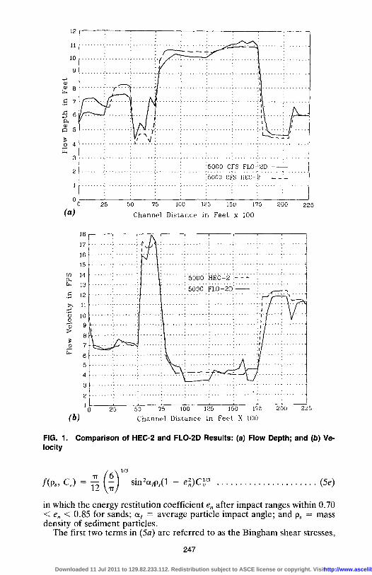
FIG. 1. Comparison of HEC-2 and FLO-2D Results: (a) Flow Depth; and (b) Ve- locity

f(p,, Cv) = ]-~ sin2c~,ps(1 - - p2](~'1/3 (5e) v n ] v v . . . . . . . . . . . . . . . . . . . . . .

in which the energy restitution coefficient e, after impact ranges within 0.70 < e, < 0.85 for sands; at = average particle impact angle; and Ps = mass density of sediment particles.

The first two terms in (5a) are referred to as the Bingham shear stresses,

247


FIG. 2. Rudd Creek Alluvial Fan Topography

and represent the internal resistance stresses of a Bingham fluid. The sum of the yield stress and viscous stress defines the shear stress of a cohesive, hyperconcentrated sediment fluid in a viscous flow regime. The last term represents" the sum of the dispersive and turbulent shear stresses, which depends on the square of the vertical velocity gradient. A discussion of these stresses and their role in hyperconcentrated sediment fows can be found in Julien and O'Brien (1987).

A mudflow model that incorporates only the Bingham stresses, and ig- nores the inertial stresses,, assumes that the simulated mudflow is viscous. This assumption is not generally applicable, because all mud floods and some mudfows are turbulent, with velocities as high as 8 m/s (25 fps). Even flows considered as mudflows with concentrations up to 40% by volume can be turbulent (O'Brien 1986). Depending on the fluid matrix properties, viscosity and yield stresses for concentrations up to 40% can still be relatively small compared to the turbulent stresses at high velocities.

To define the terms in (5a) for use in the FLO-2D model, the following approach was taken. By analogy with the work of Meyer-Peter and Mfiller (1948) and Einstein (1950), the shear stress relationship (4) is depth-inte- grated and rewritten in the following sIope form

S~ = S~ + S~ + S,. . . . . . . . . . . . . . . . . . . . . . . . . . . . . . . . . . . . . . . . . . . (6 )

in which the total friction slope S s = sum of the components: the yield slope Sy; the viscous slope St.; and the turbulent-dispersive slope Sta. The viscous and turbulent-dispersive slope terms are written in terms of depth-averaged velocity V. The viscous slope can be written as

K.qV Sv - 8~,, h ~ . . . . . . . . . . . . . . . . . . . . . . . . . . . . . . . . . . . . . . . . . . . . . . . . (7)

in which "y,~ = specific weight of the sediment mixture. The resistance parameter K for laminar flow equals 24 for smooth, wide, rectangular channels, but increases with roughness and irregular cross section geometry.

248


FIG. 3. Rudd Creek 1983 Mudflow Boundary

The flow resistance of the turbulent and dispersive components of (7) are combined into an equivalent Manning n value for the flow

F/2V2 Sta- h4/3 . . . . . . . . . . . . . . . . . . . . . . . . . . . . . . . . . . . . . . . . . . . . . . . . . ( 8 )

Accordingly, the friction slope components can be written as

% K'qV n2V 2 s~-- ~mh + ~ + h 4,---v . . . . . . . . . . . . . . . . . . . . . . . . . . . . . . . . . . . (9)

The velocity is computed across each grid boundary using the average flow depth between two adjacent elements. Reasonable values of K and Manning n can be assumed for the channel and overland flow roughness. The specific weight of the fluid matrix 7,n increases with sediment concert-

249


10000

9000

8000

7ooo! 6000

5000 1

4000

3 0 0 0

2000

lO00

RUDD CREEK MUDFLOW

/ !

I r l

I I

I I I I

r ~ ! I

HYDROGRAPH

/ CC NC. BY VOL / %

I

CHARGE (Ci q ~)

~ L i00 200 300 400

TIME (SECONDS)

FIG. 4. Rudd Creek Mudflow Hydrograph

500 600

5o / . r,,

49 ~ r~-

4~

4v ~ C >

46 .

45 ,~ c

44 ~

4a ~

c 42 ~-

700

FIG. 5. Mudflow Frontal Deposit (Courtesy of USDA Soil Conservation Service, Salt Lake City)

250


FIG. 6. FLO.2D Grid System and Location of Principal Streets and Buildings

tration. The yield stress Ty and the viscosity "q vary principally with sediment concentration. The following empirical relationships can be selected, unless a rheological analysis of the material is available:

= e q e ~ , C ~ . . . . . . . . . . . . . . . . . . . . . . . . . . . . . . . . . . . . . . . . . . . . . . . . (10) and

Ty = ~ z e ~-c~ . . . . . . . . . . . . . . . . . . . . . . . . . . . . . . . . . . . . . . . . . . . . . . . (11)

in which c~i and [3i = empirical coefficients defined by laboratory experiment (O'Brien and Julien 1988). The viscosity and yield stress are shown to be functions of the volumetric sediment concentration C~, of silts, clays, and in some cases, fine sands, and do not include larger elastic material rafted along with the flow.

251


CONTOUR INTERVAL = 2 FT

"~

RU

DD

~

....

... -

~s

J C

RE

EK

\

(a)

l ~t GR

APHIC

SC

AL

E

(IN F

t%"r.

I F'

r ffi

0.30

5 m

) _

T (b

)

CR

EE

K

7

CONTOU

R INTER

VAL =

2

FT

(0.6

1 m

)~sfL ~

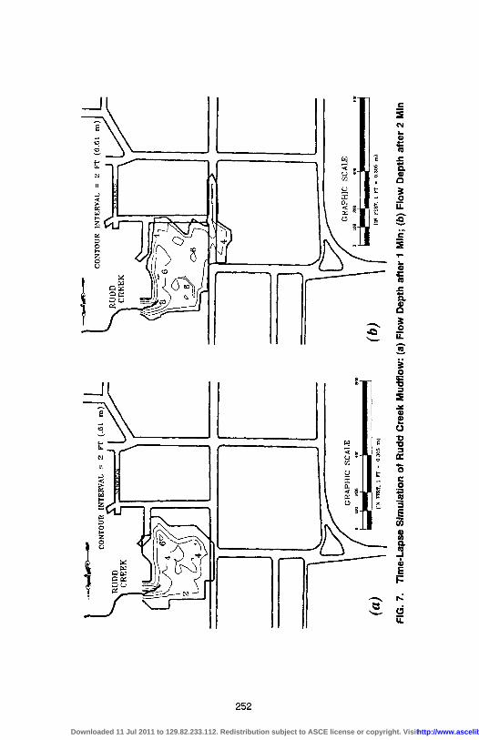
FIG

. 7.

Tim

e-La

pse

Sim

ulat

ion

of R

udd

Cre

ek M

udflo

w:

(a)

Flow

Dep

th a

fter

1 M

in;

(b)

Flow

Dep

th a

fter

2 M

in


r~

! -~

-

co.o

uR ,

~vA

~ :

~ ~

Io~

J__

(c)

RUDD

L CREEK !k

CONT

OUR

INTE

RVAL

= ~

FT

(0.6

i) L

-S

G RA

PI-~

IC S

C ~LF

= i

i .

..

..

.

)

(d)

(iN .E

'r ...

....

. ,

FIG

. 7.

(Con

tinue

d) T

ime-

Laps

e S

imul

atio

n of

Rud

d C

reek

Mud

flow

: (c

) Fl

ow D

epth

aft

er 3

Mln

; (d

) Fl

ow D

epth

aft

er 5

Min


~)

(b)

FIG. 8. 3-D Graphic Presentation of Time-Lapse Simulation: (a) Flow Depth after 1 Min; (b) Flow Depth after 2 Min

FLO-2D MODEL DESCRIPTION

The FLO-2D model evolved from the diffusive hydrodynamic model (DHM) (Hromadka and Yen 1987). The original DHM routing algorithm was re- vised and expanded to improve computational stability, decrease computational time, and broaden its application to more diverse flooding conditions. Very little of the original code remains.

The model uses a central finite difference routing scheme (an explicit numerical technique) for the application of the equations of motion. The surface topography is discretized into uniform square-grid elements. Each element is assigned a location on the grid system, an elevation, a roughness factor, and area and flow width reduction factors used to simulate flow blockage.

Flow is routed through the grid system using estimates of the flow depth to compute discharge. For a given element and time step, the discharge across each of the four boundaries is computed and summed. The resultant volume change is uniformly distributed over the available flow area in the element. Time steps vary according to the Courant-Friedrich-Lewy stability condition (Liggett and Cunge 1975), resulting in relatively short time steps (e.g., 1-30 s).

254


(d)

FIG. 8. (Continued) 3-D Graphic Presentation of Time-Lapse Simulation: (c) Flow Depth after 3 Min; (d) Flow Depth after 5 Min

Mass conservation is maintained for both the water and mudflow sediment volumes as the flow hydrograph is routed over the grid system. When routing mudflows, the sediment continuity is preserved by tallying the sediment volume for each grid element; thus tracking the sediment volume through the grid system. At each time step, the model computes the change in water and sediment volumes, and the corresponding change in sediment concentration.

Flow cessation is simulated with the potential for remobilization. For mudflows, high sediment concentrations result in a very viscous flow, which may halt on mild slopes. When successive discharges of less sediment concentration enter a grid element with a halted flow, the diluted mixture may remobilize.

The accuracy of FLO-2D hydraulic computations for steady flow was verified through a comparison with field data and replication of HEC-2 results for contained channel flow, as shown in Fig. 1. Both water surface and velocity results were compared using similar data files for a variable area channel and alternating subcritical and supercritical slope reaches ex- tending over 6.4 km (4 mi). Separate HEC-2 runs were required for the subcritical and supercritical flow regimes. The HEC-2 predicted water surface was estimated in the flow transition locations. Additional information on model verification is available in O'Brien and Fullerton (1990).

255


RUDD L CREEK

1983 MUDFLOW BOUNDARY (COE) ,

J

800 | # 0

" CONTOUR INTERVAL = 2 FT GRAPHIC SCALE

100 200 400 800

( IN FEE~ )

FIG. 9. Rudd Creek Mudflow Simulation after 15 Min

MODEL LIMITATIONS AND ASSUMPTIONS

Wave attenuation in the diffusive model is the resuk of overbank storage and the interaction of the friction slope and diffusive pressure gradient terms with the bed slope. The present model does not have the ability to simulate shock waves or hydraulic jumps, and tends to smooth out these abrupt changes in the flow profile.

The inherent assumptions in applying the model for flood routing are: (1) Steady flow for the duration of the time step (usually a few seconds); (2) hydrostatic pressure distribution; (3) steady flow resistance equation; (4) sufficiently uniform cross section shape and hydraulic roughness of the channel; and (5) single values of grid-element elevation and roughness.

In addition, FLO-2D is a rigid bed model and does not simulate degra- dation. This is not a serious limitation for urban floodplain flow (less erodible

256


RUDD CREEK

1983 MUDFLOW BOUNDARY (cos) ,

CONTOUR INTERVAL

,/ ,W

LI

V

I "I / GRAPHIC SCALE lOO 200 i .00 t I I 400 800

( ]N FEET )

FIG. 10. Rudd Creek Mudflow Simulated Maximum Flow Depth Contours

surfaces) and depositional flows such as mudflows, which may cease flowing when obstacles are encountered.

The detail and accuracy of a flood simulation is related to grid size. A grid size of 30-150 m (100-500 ft) is usually appropriate for detailed simulations. Finer grid resolution requires more computer run time, more ex- tensive data files, and more detailed boundary conditions.

CASE STUDY~1983 RUDD CREEK MUDFLOW

Model simulation of water flooding through urban areas with channels and streets has produced excellent results (O'Brien and Fullerton 1990). The simulation of mud or debris flow requires more engineering judgment. To demonstrate FLO-2D's capability to model mudflows, the 1983 Rudd Creek mudflow in Davis County, Utah, is presented. Figs. 2 and 3 show

257


the approximate boundary of the mudflow after the flow had ceased, as indicated by the U.S. Army Corps of Engineers (Incorporating 1986). Close examination of photos taken after the event shows that the boundaries of the deposit were slightly more irregular than shown in Figs. 2 and 3, but the correlation is reasonable.

The flood hydrograph and other pertinent data used in the simulation were published by the U.S. Army Corps of Engineers (Incorporating 1986).The hydrograph is shown in Fig. 4. Available field data from the event included: (1) The area of inundation indicated from photography; (2) a surveyed volume of the mudflow deposit of approximately 64,200 m 3 (84,000 cu yd); (3) mudflow frontal velocity on the alluvial fan of approximately the speed that a man could walk [0.6-1.2 rrds (2-4 fps), eyewitness account]; and (4) observed mudflow depths that ranged from approximately 3.7 m (12 ft) at the apex of the alluvial fan to approximately 0.6-0.9 m (2-3 ft) at the debris front (Fig. 5).

The mudflow was initiated by a landslide, and therefore a relatively uniform sediment concentration was assumed, which increased slightly as the event progressed to simulate dewatering (Fig. 4). Manning n roughness values for each grid element varied from 0.035 to 0.10, depending on veg- etation and flow obstruction. Appropriate values from laboratory data were selected for et i and [3i in (10) and (11) to compute viscous and yield stresses. The buildings that influenced the flow path were modeled, and their location is shown in Fig. 6.

A time-lapse simulation of the progression of the mudflow over the Rudd Creek alluvial fan is illustrated in Fig. 7. Time-sequence flow depths are written to files for a CAD graphics program that plots the depth contours. With the plotting package, the flood hazard delineation is automated. When the viscous flow encounters a street with a favorable slope, it proceeds ahead of the main body of the flow, as shown for the 2 min and 5 min simulation times in Fig. 7. A 3-dimensional graphic display of the time-lapse simulation, as viewed from the upstream direction, is shown in Fig. 8. The 3-D view helps to visualize how the mud piles up near the fan apex. Postevent photos revealed that houses in this vicinity received the most damage.

The hydrograph in Fig. 4 indicates that the flood event was over in less than 7 min. The model predicted that the mudflow continued to creep down the fan for several more minutes before flow cessation. By the end of 15 rain, all the flow on the fan had ceased (Fig. 9). There is little difference in the mudflow boundary after 15 min (Fig. 9) and the boundary for the 5 min simulation (Fig. 7).

The maximum computed flow depth of 3.6 m (11.8 ft) downstream of the apex compared well with the 3.7 m (12 ft) observed depth (Fig. 10). Mudflow velocities predicted on the fan ranged from 0.3 to 1.2 m/s (1-4 fps) or approximately walking speed, as was observed. Near the fan apex, maximum predicted velocities were less than 3.0 m/s (10 fps). Just upstream of the apex in the Rudd channel area, predicted velocities exceeded 6.1 m/s (20 fps). Predicted frontal lobe depths ranged from 0.6 to 1.2 m (2-4 ft), depending on the location on the fan, and correlated well with postevent photos.

CONCLUSIONS

The two-dimensional model FLO-2D is a flexible tool to augment the capability of the floodplain manager and engineer to predict flood hydraulics, identify areas of inundation, and design options for flood containment.

258


The model has components to enhance the prediction of floodplain or alluvial fan flooding including flood hydrograph routing, prediction of street flow, and mudflow simulation. Urban flood simulation has been improved by modeling flow-path obstruction and storage loss due to buildings and flood-containment walls.

Simulation of the 1983 Rudd Creek mudflows with FLO-2D correlated well with the observed area of inundation, maximum flow depth at the fan apex, frontal wave flow depths, and velocities and final deposits based on mudflow cessation. Mudflow in streets was predicted to advance in front of the main flow body, while building obstructions caused increased flow depth near the fan apex.

APPENDIX I. REFERENCES

Akan, A. O., and Yen, B. C. (1981). "Diffusion-wave routing in Channel Networks." J. Hydr. Div., ASCE, 107(6), 719-732.

Bagnold, R. A. (1954). "Experiments on a gravity-free dispersion of large solid spheres in a Newtonian fluid under shear." Proc., Royal Society of London, series A, 225, 49-63.

DeLeon, A. A., and Jeppson, R. W. (1982). "Hydraulic and numerical solutions of steady-state but spatially varied debris flow." Hydraulics and hydrology series, UWRL/H-82/03, Utah State Univ., Logan, Utah.

Egashira, S., Ashida, K., Yajima, H., and Takahama, J. (1989). "Constitutive equations of debris flow.'" Ann., disaster prevention res. inst., No. 32B-2, Kyoto Univ., Kyoto, Japan, 487-501.

Einstein, H. A. (1950). "The bed-load function for sediment transportation in open channel flows." USDA tech. bull. no. 1026, U.S. Department of Agriculture, Washington, D.C.

FAN, an alluvial fan flooding computer program, user's manual. (1990). Federal Emergency Management Agency, Office of Risk Assessment, Washington, D.C.

Hromadka, T. V. II, and Yea, C. C. (1987). "Diffusive hydrodynamic model." Water Resources Investigations Report 87-4137, USGS, Denver Federal Center, Denver, Colo.

Incorporating the effects of mudflows into flood studies on alluvial fans. (1986). U.S. Army Corps of Engineers, Omaha District, Omaha, Ne.

Julien, P. Y., and Lan, Y. Q. (1991). "On the theology of hyperconcentration." J. Hydr. Engr., ASCE, 117(3), 346-353.

Julien, P. Y., and O'Brien, J. S. (1987). "Discussion of "Mountain torrent erosion." Sediment transport in gravel-bed rivers. John Wiley & Sons, New York, N.Y., 537-539.

Liggett, J. A., and Cunge, J. A. (1975). "Numerical methods of solution of the unsteady flow equations." Unsteady Flow in Open Channels, K. Mahmood and V. Yevjevich, eds., Water Resources Publications, Fort Collins, Colo.

MacArthur, R. C., and Schamber, D. R. (1986). "Numerical methods for simulating mudflows." Proc., 3rd Int. Symp. on River Sedimentation, Univ. of Mississippi, Oxford, Miss., 1615-1623.

Major, J. J., and Pierson, T. C. (1990). "Rheological analysis of fine-grained natural debris-flow material." Proc., Int. Symp. on Hydr./Hydro. of Arid Lands, ASCE, New York, N.Y., 225-231,

Meyer-Peter, E., and Mtiller, R. (1948). "Formulas for bedload transport." Proc., IAHRM 2nd Congr., Int. Assoc. for Hydr. Res., Stockholm, 39-64.

O'Brien, J. S. (1986). "Physical processes, rheology and modeling of mudflows," PhD thesis, Colorado State University, Fort Collins, Colo.

O'Brien, J. S., and Fullerton, W. T. (1990). "Urban floodplain and alluvial fan stormwater modeling." Urban Hydro., Proc., 26th Annual A WRA Conf., Denver, Colo.

O'Brien, J. S., and Julien, P. Y. (1985). "Physical properties and mechanics of hyperconcentrated sediment flows." Proc., ASCE Specialty Conf. on the Deline-

259


ation of Landsfides, Flash Floods and Debris Flow Hazards in Utah, Utah Water Research Lab., Univ. of Utah at Logan, Utah, 260-279.

O'Brien, J. S., and Julien, P. Y. (1988). "Laboratory analysis of mudflow properties." J. Hydr. Engrg., ASCE, 114(8), 877-887.

Ponce, V. M., Li, R. M., and Simons, D. B. (1978). "Applicability of kinematic and diffusion models." J. of Hydr. Div., ASCE, 104(3), 353-360.

Schamber, D. R., and MacArthur, R. C. (1985). "One-dimensional model for mudflows." Proc., ASCE specialty conference on hydr. and hydro, in the small comp. age. Vol. 2, ASCE, New York, N.Y., 1334-1339.

Takahashi, T., and Tsujimoto, H. (1985). "Delineation of the debris flow hazardous zone by a numerical simulation method." Proc., Int. Syrup. on Erosion, Debris Flow and Disaster Prevention, Tsukuba, Japan, 457-462.

Takahashi, T., and Nakagawa, H. (1989). "Debris flow hazard zone mapping." Proc., Japan-China (Taipei) Joint Seminar on Natural Hazard Mitigation, Kyoto, Japan, 363-372.

APPENDIX II. NOTATION

The following symbols are used in this paper:

a i

C = c~= C, --

e n

f = g =

h = i =

K = 1 =

n =

s~= s~=

S t d ~

S v -=

s ,= So~= S o y ~

t = V =

v~= v ,=

X ~

y =

~ I "~

(~-i ~

.q =

coefficient defined by Bagnold; inertial shear stress coefficient; volumetric sediment concentration; maximum static volume concentration for sediment particles; representative sediment size; particle energy restitution coefficient after impact; Darcy-Weisbach friction coefficient; gravitational acceleration; flow depth; rainfall intensity; resistance parameter for viscous flow; Prandtl mixing length; Manning resistance coefficient; friction slope; friction slope component along x coordinate axis; friction slope component along y coordinate axis; turbulent-dispersive slope; viscous slope; yield slope; bed slope component along x coordinate axis; bed slope component along y coordinate axis; time; depth averaged velocity; velocity component along x coordinate axis; velocity component along y coordinate axis; velocity; coordinate axis; coordinate axis; average particle impact angle; coefficients of viscosity and yield stress; exponents of viscosity and yield stress; specific weight of mixture; dynamic viscosity;

260


~ r n

Ps = I" -----

T c ~---

3- d ~---

Trrlc

T t

- r r=

= mass density of mixture; sediment particle mass density; total shear stress; cohesive yield strength; dispersive shear stress; Mohr-Coulomb shear stress; turbulent shear stress; viscous shear stress; yield stress; and angle of repose of flow material.

261


by j. s. o'brien, 1 p. y. julien, 2 and w. t. fullerton, 3...

Documents