1

Buying Beauty: On Prices and Returns in the Art Market

Luc Renneboog and Christophe Spaenjers*

This version: 6 December 2011

Abstract: This paper investigates the price determinants and investment performance of art. We apply a

hedonic regression analysis to a new data set of over one million auction transactions of paintings and

works on paper. Based on the resulting price index, we conclude that art has appreciated in value by a

moderate 3.97% per year, in real U.S. dollar terms, between 1957 and 2007. This is a performance

similar to that of corporate bonds – at much higher risk. A repeat-sales regression on a subset of the data

demonstrates the robustness of our index. Next, quantile regressions document larger price

appreciations in higher price brackets. We also find variation in historical returns across mediums and

movements. Finally, we show that both high-income consumer confidence and art market sentiment

forecast art price trends.

Key words: art; auctions; hedonic regressions; investments; repeat-sales regressions; sentiment.

* Luc Renneboog (luc.renneboog@uvt.nl) is Professor of Corporate Finance, Tilburg University, the Netherlands. Christophe Spaenjers (spaenjers@hec.fr) is Assistant Professor of Finance, HEC Paris, France. The authors would like to thank Sofiane Aboura, Richard Agnello, David Bellingham, Fabio Braggion, Michael Brennan, Peter Carpreau, Geraldo Cerqueiro, Gilles Chemla, Mark Clatworthy, Craig Clunas, Peter De Goeij, Neil De Marchi, Alberta Di Guili, Elroy Dimson, Kevin Evans, Julian Franks, Rik Frehen, Edith Ginglinger, Victor Ginsburgh, Marc Goergen, William Goetzmann, Tom Gretton, Duncan Hislop, Noah Horowitz, Jonathan Ingersoll, Martin Kemp, Marius Kwint, Geraldine Johnson, Benjamin Mandel, David Marginson, Bill Megginson, Allison Morehead, Thierry Morel, Michael Moses, Kim Oosterlinck, Liang Peng, Rachel Pownall, Clara C. Raposo, Catarina Reis, Keith Robson, Frans de Roon, Geert Rouwenhorst, Ahti Salo, Sofia Santos, Marie Shushka, Mick Silver, Myron Slovin, Cindy Soo, Matthew Spiegel, Darius Spieth, Peter Szilagyi, Nick Taylor, Svetlana Taylor, Radomir Todorov, Hans Van Miegroet, Joost Vanden Auwera, Stephen Walker, Jason Xiao, Roberto Zanola, and participants at seminars and workshops at Antwerp University, Cambridge University, Cardiff Business School, Duke University, ISCTE Business School, London Business School, Manchester Business School, Paris-Dauphine University, Tilburg University, UCL-Core, Universidade Catolica Portuguesa, Universidade Nova de Lisboa, Yale University, the 2009 FMA Meetings, the 2009 LBS Annual Art Investment Conference, and the 2009 Multinational Finance Conference for valuable comments and suggestions. Spaenjers would like to thank the Netherlands Organisation for Scientific Research (NWO) for financial support, and London Business School for its hospitality.

2

I. Introduction

Stories about the baffling amounts of money paid for first-tier art frequently entertain newspaper readers

around the world. Yet, high prices do not necessarily imply high returns. Consider, for example, Claude

Monet’s “Dans la Prairie”, the star lot of the Impressionist and Modern Art Evening Sale at Christie’s

London in February 2009. The canvas changed owners for the substantial sum of 10 million British Pound

(GBP), and was the top seller in an auction that, according to the Wall Street Journal (2009), “showed that

there's plenty of life” in the Impressionist and Modern sector. However, the same painting had been sold

twice before in recent history – in June 1988 at Sotheby’s London for 14.3 million GBP, and in November

1999 at Sotheby’s New York for 15.4 million U.S. dollars (USD). By any standard, the rate of return on the

Monet was dismal.

Nevertheless, the growth in the number of multi-million dollar sales, the expansion of the global

population of high-net-worth individuals, and the increasing need for portfolio diversification have all

brought increased attention to art as an investment in recent years. In turn, the belief in art as a viable

alternative asset class has led to the creation of several art funds – not all very successful (Horowitz, 2011)

– and art market advisory services which cater to affluent individuals who consider investing in art. The

Wall Street Journal (2010) recently reported that almost 8% of total wealth is held in so-called “passion

investments”: art, musical instruments, wine, jewelry, antiques, etc. Of all such luxury assets, art is the most

likely to be acquired for its potential appreciation in value (Capgemini, 2010).

There is a growing academic literature on art investments, but previous studies have utilized relatively

small data sets of sales (pairs) at the high end of the market. The resulting indices are prone to a number of

estimation issues and selection biases (cf. Section II). The current paper therefore uses a comprehensive

new data set of nearly 1.1 million auction sales to re-examine the price formation and returns in the art

market, over a period from 1957 to 2007.

We perform a hedonic regression analysis which relates transaction prices to a wide range of value-

determining characteristics and year effects. Our results show that artist reputation, attribution, signs of

authenticity, medium, size, topic, and the timing and location of the sale are significantly correlated with

price levels. Based on the regression coefficients on the year dummies in our model, we can build a price

index that controls for time variation in the composition of the market (and corrects for changes in price

dispersion). We find that constant-quality art prices increased by a moderate 3.97% in real USD terms on a

yearly basis over the 1957-2007 period. Between 1982 and 2007, the geometric average annual real return

is 5.19%. For the second half of the twentieth century, our estimates are substantially below those reported

by Goetzmann (1993) and Mei and Moses (2002).

Our baseline hedonic index proves robust to alternative specifications and estimation methods. For

example, allowing for time variation in the hedonic coefficients does not materially affect our results.

3

Importantly, also applying a repeat-sales regression to a subset of our sample leads to nearly identical return

estimates for the 1982-2007 period. Quantile regressions over the same time frame show that historical

rates of appreciation vary across the price distribution; the annualized real return at the 95th percentile is

almost 5 percentage points higher than the return at the 5th percentile. In line with this finding, but in

contrast to previous research (and to what the Monet example may suggest), we do not find that portfolios

of masterpieces underperform the rest of the market. Moreover, a “value” strategy, in which one focuses on

important but relatively less expensive artists, has outperformed our baseline index by 1.6 percentage points

on an annualized basis. Next, we show that oil paintings and post-war movements have outperformed other

art over the last few decades.

Overall, the risk-return profile of art has been inferior to that of financial assets, even before transaction

costs, especially in the second half of our time frame. However, art has outperformed other physical assets,

such as gold, commodities, and real estate. While we find a low correlation between changes in the art price

index and same-year equity returns, the correlation with lagged equity returns is substantially higher.

Finally, we examine the determinants of art market returns. We find evidence that (lagged) equity

market returns and changes in high-income consumer confidence predict art returns, highlighting the

importance of luxury consumption demand. However, we document that also a novel art buyer sentiment

measure (based on volume and buy-in rates at high-profile auctions, and on media reports) forecasts price

changes. This suggests that time-varying optimism about the potential of ‘art as an investment’ can partially

explain the existence of art market cycles.

II. Literature on art returns

Researchers have used different methodologies to calculate the financial returns on art investments, starting

from public auction records.1 Stein (1977) considers the auctioned objects in each year as a random sample

of the underlying stock of art (by deceased artists), and constructs an index based on the yearly average

transaction price. Baumol (1986) and Frey and Pommerehne (1989) calculate the geometric mean return on

works that sold at least twice during the considered time frame. Unfortunately, however, these simple

methods do not enable the construction of a price index that adjusts for variations in quality. Most recent

studies have therefore used either repeat-sales regressions or hedonic regressions to measure the price

movements of art and other infrequently traded assets (e.g., real estate).

Repeat-sales regressions (RSR) explicitly control for differences in quality between works by only

considering items that have been sold at least twice. The method uses purchase and sale price pairs to

1 Art is not only sold at auction, but also privately, for example through dealers. Total turnover in the art and antiques market is roughly split equally between the two transaction types (McAndrew, 2010). However, it is generally accepted that auction prices set a benchmark also used in the private market.

4

estimate the average return of a portfolio of assets in each time period. Pesando (1993), Goetzmann (1993),

Mei and Moses (2002), and Pesando and Shum (2008), among others, have applied the methodology to art

investments. There are three problems with existing RSR studies. First, since art objects trade very

infrequently (and resales can be hard to identify), only considering repeated transactions decimates any data

set to a relatively small number of observations. For example, Mei and Moses (2002) include 4,896 sales

pairs over a period of 125 years; Goetzmann et al. (2011) use even fewer sales pairs, although their focus is

not on the resulting price index itself. Meese and Wallace (1997) show that the use of such small databases

renders RSR estimators sensitive to influential observations. Second, most repeat-sales studies suffer from

selection issues. For example, the sample used by Mei and Moses (2002) includes sales pairs with a first

transaction anywhere in the world, but a resale at Sotheby’s or Christie’s New York – arguably the most

expensive sales rooms in the world. Moreover, the initial purchase is identified using the provenance entries

in the New York sales catalogues; this information could be more likely to be included when a high price is

expected. An index estimated based upon such a sample may thus be biased upwards. Other studies,

including Goetzmann (1993), have utilized repeat-sales information from the so-called “Reitlinger data” –

books with auction price data until the 1960s – of which is well known that they are incomplete and focus

disproportionately on famous artists (Guerzoni, 1995). Third, even abstracting from the issues just outlined,

items which trade twice may in general not be representative for the overall population of art works.

Hedonic regressions control for quality changes in the transacted goods by attributing implicit prices to

their “utility-bearing characteristics” (Rosen, 1974). In the often-used time-dummy variant of the hedonic

pricing methodology, all available transaction data are pooled, and prices are regressed on a set of value-

determining attributes and one or more time dummies. Under the assumption that all omitted characteristics

are orthogonal to those included (Meese and Wallace, 1997),2 the coefficients on the time dummies account

for constant-quality price trends over the sample period. Since no information is thrown away prior to the

estimation, hedonic regressions make efficient use of available data, and may therefore give more reliable

estimates of price indices than RSR. Not surprisingly, one of the key difficulties is the choice of hedonic

characteristics (Ashenfelter and Graddy, 2003). Observable and easily quantifiable features such as size,

medium, and the location of sale are frequently used (Anderson, 1974; Buelens and Ginsburgh, 1993;

Chanel et al., 1996; Agnello and Pierce, 1996), but the number of hedonic variables often remains relatively

limited. The literature has failed to systematically include variables that measure reputation or the strength

of attribution, an important price-determining factor for Old Masters (Robertson, 2005). Also, just like in

studies using RSR, the utilized samples have been relatively small and selective. Research has been based

2 Although there are omitted variables in every model, hedonic pricing is particularly suitable for luxury consumption goods markets, in which a limited number of key characteristics often determine the willingness to pay for an item (e.g., the 4 Cs of a diamond). In any case, Butler (1982) argues that the omitted variable bias is often negligible; “approximate correctness can be achieved with significantly fewer characteristics than is generally supposed”.

5

either on the problematic (and old) Reitlinger data mentioned before (Buelens and Ginsburgh, 1993; Chanel

et al., 1996), or on samples of art from one country (Agnello and Pierce, 1996; Renneboog and Van Houtte,

2002; Higgs and Worthington, 2005).

The estimated returns on art vary with data, methodology, and the time period under consideration

(Ashenfelter and Graddy, 2003). With respect to paintings, the two most influential repeat-sales studies

report relatively high real returns over the second half of the twentieth century. Goetzmann (1993)

calculates an average annual real appreciation of 3.8% between 1850 and 1986, but with a “long and

strong” bull market, in which annualized returns average around 15%, since 1940. Mei and Moses (2002)

reports a real return of 4.9% over the period 1875-1999, but a higher annualized return estimate of 8.2%

after 1950. (For prints, Pesando and Shum (2008) report much lower returns over the period 1977-2004.) In

general, studies that use hedonic regressions have found somewhat lower returns, but to date no exhaustive

hedonic analysis has been undertaken.

III. Data and methodology

In this paper, we construct a price index for art using the hedonic regression methodology. As outlined

before, the main advantage of this approach is that information on all observed transactions can be taken

into account. Our model relates the natural logs of real USD prices to year dummies, while controlling for a

wide range of hedonic characteristics:

∑ ∑= =

+++=M

m

T

tktkttmktmkt DXP

1 1ln εγβα (1),

where Pkt represents the price of art object k at time t, Xmkt is the value of characteristic m of item k at time t,

and Dkt is a time dummy variable that takes the value one if object k is sold in period t (and zero otherwise).

The coefficients βm reflect the attribution of a relative shadow price to each of the m characteristics, while

the antilogs of the coefficients γt can be used to construct an art price index that controls for time variation

in the quality of art sold. The value of the hedonic index in year t is:

100*)exp( tt γ≡Π

(2),

with γ0 set equal to 0 for the initial, left-out period. The return in year t is then:

11

−ΠΠ

≡−t

ttr

(3).

However, a subtle (and often neglected) point is that such an index will track the geometric – not the

arithmetic – mean of prices over time, due to the log transformation prior to the estimation. This is

especially important for our estimation of returns if there is time variation in the heterogeneity-controlled

dispersion in prices, i.e., the hedonic regression residuals (Silver and Heravi, 2007). If we assume that the

6

residuals of our hedonic regression are normally distributed in each period, with variance 2tσ in period t,

then we can correct for this transformation bias by defining the corrected index values as follows (Triplett,

2004; Silver and Heravi, 2007):

100*)(21exp 2

02*

−+≡Π σσγ ttt

(4).

The corrected return in year t, can then be defined as follows:

1*1

** −

ΠΠ

≡−t

ttr

(5).

We describe our data in subsection A. The hedonic variables that will be used in the estimation of Eq.

(1) are presented in subsection B.

A. Data

We focus on the market for oil paintings and works on paper (i.e., watercolors and drawings), which

account for a substantial proportion of all transactions – and about 85% of total turnover – in the art market

(Artprice, 2006). We start by compiling a list of artists. This selection of artists has to be as exhaustive as

possible, so as not to have a bias towards artists that are popular today, and therefore we consult several

authoritative art history resources from different time periods. Our artist selection procedure, of which

details can be found in Appendix A, culminates in a list of 10,442 artists. We classify 4,490 of those artists

in at least one of the following art movements: Medieval & Renaissance; Baroque; Rococo; Neoclassicism;

Romanticism; Realism; Impressionism & Symbolism; Fauvism & Expressionism; Cubism, Futurism &

Constructivism; Dada & Surrealism; Abstract Expressionism; Pop; Minimalism & Contemporary.

We then collect data on all relevant sales by matching our list of names with all artists in the online

database Art Sales Index [http://www.artinfo.com/artsalesindex]. This resource contains auction records for

different types of art. Prices are hammer prices, exclusive of transaction costs. Historically, the Art Sales

Index, just like many other databases, has not included buy-ins (i.e., items that do not reach the reserve

price and remain unsold).

Although the first sales in the Art Sales Index date from the beginning of the 1920s, data are unavailable

or sparse in many years until the second half of the 1950s. Therefore, we start our analysis in 1957, the first

year for which we have more than 1,000 observations. (Unfortunately, however, for 1963 the data coverage

is limited, with only some of the highest priced sales included.) The Art Sales Index only includes London

sales until the late 1960s, but it has an exhaustive worldwide coverage afterwards. The most recent auction

records available for this study are from the autumn auctions of 2007.

Our final data set consists of 1,088,709 sales; about 60% of these transactions concern oil paintings,

with the remainder split roughly evenly between watercolors and drawings. The artist with the highest

7

numbers of sales (5,405) is Pablo Picasso. The magnitude of our database enables us to draw a complete

picture of the price formation and the returns in the art market, in contrast to most previous studies which

are based on more selective samples.

We translate all nominal prices in our data set to prices in year 2007 USD, using the CPI as a measure of

inflation. In real terms, the most expensive transaction is ‘Portrait du Dr. Gachet’ by Vincent van Gogh,

which sold for 75 million USD in May 1990 at Christie's New York. (In nominal prices, it is ‘Garçon à la

Pipe’ by Pablo Picasso, which was auctioned off for 93 million USD in May 2004 at Sotheby's New York.)

While such high-profile sales attract ample attention, the average price level is much lower. The mean

(resp. median) sales price over all observations for 2007 is 159,354 USD (resp. 14,775 USD).

Goetzmann (1996) argues that survivorship could cause upward bias in the estimation of art returns,

since artists who “fall from fashion” are typically not traded. The impact of this bias on our results may be

rather small. First, as Goetzmann (1996) points out himself, the rate of artist obsolescence is relatively low.

Second, in contrast to previous work, we do not require a work of art to trade twice and/or to sell at a large

auction house. Our sample thus also includes many sales of less popular artists at smaller auction houses at

any point in time (especially after 1970). Finally, pieces that are donated to museums after a substantial

increase in an artist’s fame – or items that are sold through private transactions in the early part of artists’

careers – are not observed at auction either (Goetzmann, 1993; Mei and Moses, 2002), partially offsetting

the upward bias. Nevertheless, our return estimate should probably still be considered as an upper bound on

the rate of return (before transaction costs) realized by art investors over our time frame.

B. Variables

Our hedonic regressions include a number of variables that capture the characteristics of the artist, of the

work, and of the sale. The descriptive statistics for these hedonic variables are presented in Table 1.

[Insert Table 1 about here]

First, in addition to artist dummies capturing each artist’s uniqueness, we consider the following

exogenous reputational measure:

Textbook dummy. We manually check which of our artists were included in several editions of the

classic art history textbook ‘Gardner’s Art Through the Ages’ (1926, 1959, 1980, 1996, and 2004). In

total, 652 of our artists are listed in at least one edition. The dummy variable TEXTBOOK equals one if

the artist was featured in the edition of – or the last edition prior to – the year of sale.

Two other characteristics related to the artist’s career are included in the late-twentieth-century movement-

specific models (cf. Section IV.E), but not in our general models, as they could potentially pick up price

differences between various eras or movements:

8

Exhibition dummy. The variable EXHIBITION equals one once the artist has been represented at

Documenta in Kassel. Inclusion in this prestigious exhibition evidences an artist’s rise to fame. In

total, 680 of our artists were represented at one of the eleven exhibitions between 1955 and 2002.

Dead artist dummy. It is often assumed that prices for art works increase after the death of an artist.

The dummy variable DECEASED, which equals one if the sale occurs subsequent to the artist’s

death, should capture this effect.

Second, we also consider a range of price-determining variables that capture the attribution and

authenticity, the medium, the size, and the subject matter of the work of art:

Attribution dummies. Attribution can be an important factor influencing the price of art objects,

especially of older works. Different levels of attribution are used in the auction world:

ATTRIBUTED (to), STUDIO (of), CIRCLE (of), SCHOOL (of), AFTER, and (in the) STYLE (of).

About 12% of the observations in our sample carry such an attribution.

Authenticity dummies. More than half of the art works is SIGNED, while about one third is DATED.

Medium dummies. We introduce dummies for the different medium categories: OIL,

WATERCOLOR (including gouaches), and DRAWING.

Size. The height and width in inches are represented by HEIGHT and WIDTH (with squared values

HEIGHT_2 and WIDTH_2). The average work has a height and a width of about 20 inches (51 cm).

Topic dummies. The subject matter can significantly affect the aesthetic appreciation of art objects.

We therefore categorize the works in different topic groups based on the first word(s) of the title. We

create eleven categories, based on the search strings listed in Appendix B: ABSTRACT, ANIMALS,

LANDSCAPE, NUDE, PEOPLE, PORTRAIT, RELIGION, SELF-PORTRAIT, STILL_LIFE,

UNTITLED, and URBAN. Furthermore, we create a dummy STUDY that equals one if the title

contains the words “study” or “etude”. The largest categories are portraits and landscapes.

Third, we include dummies that indicate the timing of the sale, and the reputation and location of the

auction house:

Month dummies. Since important sales are often clustered in time, we include month dummies. The

busiest months are May, June, November, and December.

Auction house dummies. We make a distinction between different fine art auction houses that have

been important throughout our sample period. For Sotheby’s and Christie’s, we introduce dummy

variables for their London, New York, and other sales (e.g., SOTH_LONDON, SOTH_NY, and

SOTH_OTHER). Together, these two institutions are responsible for about half of all sales in our

sample. For two other big British auction houses, Bonhams and Phillips, we make a distinction

between their London sales rooms and other activities (e.g., BON_LONDON and BON_OTHER).

9

We also create two dummies to account for the sales by important European and American auction

houses (AUCTION_EUROPEAN and AUCTION_AMERICAN) – see Appendix C.

IV. The returns on art

A. Baseline indices

Table 2 shows the parameter estimates of the hedonic variables for our baseline model. Eq. (1) is estimated

using ordinary least squares (OLS) and the dependent variable is the natural log of the real price in USD.

For 1,078,482 sales we have complete information on all hedonic characteristics presented in the previous

section. Because of the very large number of observations, nearly all coefficients are statistically highly

significant. Hence, we focus on economic significance as well: Table 2 shows the “price impact” of each

hedonic variable, which can be proxied by taking the exponent of the coefficient, and subtracting one. It is

important to note that the variables are in most cases picking up otherwise unobservable differences in

quality, and that the regression coefficients thus reflect correlation instead of causality. For example, works

sold at Sotheby’s or Christie’s mainly catch higher prices because of their high attractiveness, not

necessarily because of auction house certification.

[Insert Table 2 about here]

Table 2 reveals that works are on average priced 13.5% higher after the inclusion of the artist in an

important art history reference book. Also the strength of the attribution has an important effect on the price

of an art object. Whenever an attribution dummy comes into play, the price level drops by more than 50%.

Not surprisingly, larger discounts are recorded for works that are “in the style of” or “after” a master than

for “attributed” or “studio” works. We also observe that signed and dated works carry higher prices: a

signature increases the price by as much as 31% on average, while a date adds almost 19% in value. Works

on paper are priced lower than oil paintings, and drawings are less valuable than watercolors. Furthermore,

prices increase with size, up to the point that the work becomes too large, as indicated by the negative

coefficients on the squared terms. Regarding the topic dummies, there are significant discounts associated

with studies and portraits, while self-portraits trade at a premium. The coefficients on our month-of-the-

year dummies confirm that the most expensive auctions are clustered at the ends of the spring and the

autumn. Finally, the highest prices are paid at the main offices of Sotheby’s and Christie’s.

Based on the coefficients on the time dummies and the variance of residuals in each period, we construct

both an uncorrected art price index Π, and a price index Π* that corrects for log transformation bias. The

results are reported in Table 3; the price levels in 1957 are standardized to 100. As mentioned before, the

coverage of the data is very selective for the year 1963, so we geometrically interpolate index values for

that year. (Previous studies showed very small price movements in 1963.) Table 3 indicates that the index

values have high statistical precision. In most cases, the standard deviation on the regression coefficient is

10

around 0.03, which implies tight confidence intervals around each index value. Figure 1 graphically depicts

the evolution of the indices over our time frame, and compares them to the evolution of deflated average

and median prices in our data set.

[Insert Table 3 and Figure 1 about here]

The corrected price index in Figure 1 illustrates that, in boom periods, prices can increase very fast: they

more than tripled in real terms between 1982 and 1990. The yearly increase in prices between 1985 and

1990 exceeded 23%. However, prices also rapidly decreased after 1990, and no large changes in price

levels occurred between the mid-1990s and the first years of the 2000s. In the most recent art boom period

of 2002-2007, the annual real price appreciation averaged 13.65%.

The figure documents that an index based on average or median prices would overestimate the volatility

of prices, because of the lack of control for quality differences over time. Indeed, a key contribution of this

paper is to disentangle changes in market composition from those in heterogeneity-controlled price levels.

At the same time, however, the average and median series serve as a check on the order of magnitude of the

overall price appreciation (at least over the last two-three decades, when the coverage of the data set is no

longer expanding notably). Figure 1 also illustrates the quantitative importance of the correction for the log

transformation; while the end-of-period index values are very similar, we observe marked deviations

between Π and Π* over some periods.

Annualized (i.e., geometric average) returns are reported in Panel A of Table 4. We focus on the

corrected price index. On average, art has appreciated at a yearly real rate of 3.97% between 1957 and

2007. Over the last 25 years, the geometric mean real return is somewhat higher (5.19%). The nominal

equivalents (not reported), obtained by correcting the index for the year-to-year changes in the CPI series,

are 8.21% (1957-2007) and 8.47% (1982-2007). These numbers are substantially below the return estimates

reported in Goetzmann (1993) or Mei and Moses (2002) for the periods in common. For example, over the

period 1957-1999, Mei and Moses (2002) report an annualized nominal return of 12.81%, while our index

appreciated by 7.59% on an annual basis – a difference of over 5%.

[Insert Table 4 about here]

Table 4 also reports standard deviations of the time series of annual returns. For our corrected index, the

standard deviation over the full time frame is slightly above 15%. However, we will later note that this

number still underestimates the true riskiness of art investments (cf. Section V).

B. Robustness checks

We now check the quantitative robustness of our baseline results. First, we repeat our analysis using a

number of different set-ups: (i) excluding the topic dummies (as these may capture the subject matter rather

imprecisely), (ii) excluding the more than 5,000 artists with fewer than 100 sales (as these artists are less

11

liquid), and (iii) excluding Minimalism & Contemporary art (as selection and survivorship issues may be

more of a concern for more recent artists). Panel B of Table 4 shows the uncorrected real return estimates

for 1957-2007 and 1982-2007, which can be compared to the performance of price index Π, as shown in

Panel A. Our estimates do not change substantially, with annualized price appreciations over the period

1957-2007 that differ by less than 0.05% from those reported earlier.

Second, a potential problem with the hedonic approach is that coefficients are constrained to be stable

across the whole sample window. This is a strong assumption as shadow prices of hedonic characteristics

(i.e., tastes) may change over time. An adjacent-period model can mitigate this problem: by dividing the

sample in subperiods, it enables the hedonic coefficients to fluctuate (Triplett, 2004). We apply this method

to our data set by performing a separate hedonic regression for every two consecutive years since 1982 (and

then chain-linking our returns). We restrict our analysis to the second half of our time frame, because the

methodology would underestimate the returns over the full time frame due to the expansion of coverage by

the database over the first 20-25 years. The adjacent-year model generates an uncorrected return estimate

(4.60%) that is very similar to the one we obtained from the pooled data, lending further support to our

benchmark index.

Third, the main advantage of RSR is that is controls for the uniqueness of each work. Also, in contrast to

a hedonic price index, it can be thought of as an investable index, at least in theory. Unfortunately, our data

set does not uniquely identify each artwork – let alone each repeated sale. Yet, we aim to identify multiple

transactions of the same item indirectly. We consider two items as being identical if they are from the same

artist (not from a pupil or follower), have the same dimensions, carry the same title (but not “Untitled” or

“Composition”), are of the same medium, and do not differ with respect to the presence of a signature or

date. Strikingly, this reduces the data set from 1.1 million individual transactions to 30,611 ‘repeat sales’

with a holding period of at least a year. For similar reasons as before – an RSR over the full sample would

underestimate average returns because of the focus on higher-priced items in the first half of our time frame

– we look at the 21,846 transactions between 1982 and 2007. (This number compares favorably to the size

of the databases used in previous repeat-sales studies.) In line with Goetzmann (1993) and Mei and Moses

(2002), we apply a three-stage estimation procedure on our sample of repeat sales, based on Case and

Shiller (1987). In a first step, we regress returns on a matrix (containing a row for each item and a column

for each time period) with dummy variables indicating the holding period of each item, using OLS. In a

second stage, we regress the squared residuals from the first step on an intercept and the time between sales.

In a third step, we redo the RSR, using weighted least squares, with the fitted squared residuals as weights.

The last line of Panel B of Table 4 shows that, over the time frame under consideration, the RSR implies an

average annual increase in the geometric mean price of 4.56%, compared to 4.55% for the (uncorrected)

12

hedonic regression index.3 The standard deviation is only slightly higher than before. The correlation

between the repeat-sales returns and the hedonic returns (not reported) is 0.98.

C. Quantile regressions

Despite some work on the “masterpiece effect” – which examines the question whether more expensive art

out- or underperforms the overall market (e.g., Pesando, 1993; Mei and Moses, 2002) – prior literature has

not systematically explored the potential variation of returns across price brackets. This is surprising, given

that the art market is likely to be segmented for a number of reasons. First, art is indivisible, and therefore

small investors are generally not able to invest in higher-end works. Second, wealthy individuals may be

less tempted to buy in the lower-end of the market, where works do not signal the same social status

(Mandel, 2009). Third, the more expensive parts of the market may be more prone to speculation. The

distribution of returns may thus be skewed over and above a potential masterpiece effect. In such a setting,

quantile regressions may be particularly useful (Zietz et al., 2008; Scorcu and Zanola, 2011). While OLS

regressions provide estimates for the conditional means only, non-linear quantile regressions can

characterize the entire distribution of the dependent variable (Koenker and Hallock, 2001).

We estimate price trends for the percentiles 0.95, 0.75, 0.50, 0.25, and 0.05, using the adjacent-year set-

up outlined before. (We split our sample in subperiods to avoid that the hedonic coefficients measure

variation in premiums or discounts across time rather than across price brackets). We denote the price

indices by Q95, Q75, etc. We show the results, again since 1982, in Panel C of Table 4 and in Figure 2. An

interesting pattern emerges. The low performance of Q05 is particularly striking: it has an annual growth

rate of only 1.35%, compared with 4.91% for Q50 (i.e., the constant-quality median price level). Over the

last 25 years, prices have gone up more in the higher price brackets. For example, for Q95, we record an

annualized return of 6.32%. Paired-sample t-tests on the return series (not reported) show that the

difference in (arithmetic) average return between Q05 and any of the other quantile series is statistically

significant at the 0.05 level. The outperformance of the higher quantiles is mainly due to strong price rises

in times of increasing demand for art. This finding seems in line with “superstar economics”.4 The higher

3 As with the hedonic regression, the RSR implies an index that is related to the geometric mean price in each period. Goetzmann (1992) proposes to correct for log transformation bias by adding half of the cross-sectional variance of the returns in each period to the estimated coefficient, where this variance is estimated in the second step of the Case-Shiller method. However, Goetzmann and Peng (2002) argue that the nature of the bias due to the log transformation is generally not uniform through time. There is also a danger of misspecification of the error structure (Meese and Wallace, 1997) which may lead to an overestimation of the relevant correction term. Since we are mainly interested in testing the robustness of our baseline index to a change in methodology, we compare the pre-correction indices to each other; they should give similar results. 4 In Rosen (1981), a small number of superstars earn large amounts of money, and increases in demand make the earnings distribution ever more skewed. A condition is that there is “imperfect substitution among quality

13

average growth and higher volatility of the upper price range can also be associated with increases in both

income inequality (Goetzmann et al., 2011) and the income cyclicality of high-income households (Parker

and Vissing-Jorgensen, 2010), although we do not formally test these hypotheses in this paper (because of

lack of a sufficiently long time series). In contrast, at first sight, the results seem at odds with the finding of

Mei and Moses (2002) that masterpieces underperform – an issue that we turn to next.

[Insert Figure 2 about here]

D. The performance of “masterpiece” and “value” portfolios

The quantile regression results shows that prices have generally gone up more for high-value items. To

further examine the profitability and riskiness of buying high-end art, we estimate the historical

performance of two different investment strategies, based on our repeat-sales data. First, we consider a

“masterpiece” strategy: we ‘buy’ in year t all auctioned works by the 100 artists that were most expensive

over years t-1 and t-2 (as measured by an adjacent-period hedonic regression model over those years). This

strategy comes close to how other authors have examined the masterpiece effect, although we do not select

works endogenously on realized transaction prices. Second, we implement a “value” strategy: we buy in

year t all observed works by the 100 least expensive artists over t-1 and t-2 that were nevertheless included

in the art history textbook described earlier at the start of year t-2. Such a strategy could exploit fluctuations

in taste, or a lag in appreciation by the market relative to the recognition of the artist’s art-historical

significance. (Of course, the items included in this portfolio are in general still expensive compared to the

overall sales distribution.) In both cases, we apply the RSR methodology to estimate returns; in other

words, we ‘sell’ whenever the owner sold in practice. The results are shown in Panel D of Table 4, and

compared to our earlier constructed RSR index in Figure 3.

[Insert Figure 3 about here]

We find no evidence of underperformance of a “masterpiece” strategy, which is not inconsistent with

our quantile regressions, but stands in contrast to Mei and Moses (2002).5 The described strategy yields an

annualized growth in price levels of 4.81%, compared to 4.56% for our earlier constructed RSR index. The

differentiated goods”. This is certainly the case in the art market: ten mediocre works do not add up to a single masterpiece. In a recent paper, Gyourko et al. (2006) rely on superstar economics to rationalize why the gap in house prices between “superstar cities” and less attractive locations keeps increasing over time; the authors note that “living in a superstar city is like owning a luxury good”. 5 Mei and Moses (2002) and Ashenfelter and Graddy (2003) argue that idiosyncratic overbidding and mean reversion could be one explanation for the seemingly negative effect in studies that identify masterpieces based on transaction prices. Goetzmann (1996) provides an alternative explanation: if only larger auction houses are taken into account, expensive items that drop in value are more likely to be included in the sample than lesser-quality works that underperform. Of course, the relative performance of masterpieces may also vary over time, for example if it depends on evolutions in aggregate demand or the income distribution (cf. supra).

14

“masterpiece” strategy realized strikingly high returns in the boom in the late 1980s (when indeed “blue

chip” art was very much in favor), but lost much in the subsequent bust. For the “value” strategy, we record

an annualized return of 6.16%; it has performed notably well since the mid-2000s. Both high-end strategies

thus have end-of-period index values above those for the overall sample, although the outperformance is

not statistically significant at the traditional levels. The (unreported) p-value of a t-test on the difference

between the “value” returns and the benchmark returns is 0.14.

E. Indices per medium and per movement

We now return to our baseline hedonic model and repeat the hedonic regression analysis on three

complementary subsamples of our data set: oil paintings, watercolors, and drawings. The coefficients on the

hedonic variables (not reported) are in line with the previous results. Although the trends are similar across

the different types of art, we find faster price increases for oil paintings. In real terms, watercolors and

drawings were on average still priced lower in 2007 than in 1989 and 1990. Panel E of Table 4 reports the

(corrected) returns over the different time frames. Over the last half century, prices for oil paintings have

appreciated at a yearly average real rate of 4.63%, while watercolors and drawings have increased by

3.67% and 2.51% annually. Oil paintings have strongly and significantly outperformed works on paper in

the second half of our time frame – a finding that is related to the discrepancies in returns between price

categories reported before. The lower performance of art items other than paintings is also consistent with

Pesando and Shum (2008), who find an average real return on prints of 1.51% between 1977 and 2004.

Finally, we run a separate hedonic regression for each movement, based on the classification of each

artist. We add the variables EXHIBITION and DECEASED to the models for the three most recent art

movements (Abstract Expressionism, Pop, and Minimalism & Contemporary). Most artists of these

movements have been active over our time frame, which will enable a correct measurement of exhibition

and death effects. We find that EXHIBITION is significantly positive in the Abstract Expressionism and

Minimalism & Contemporary set-ups; in the latter model we also observe a clearly positive death effect

(not reported). In general, the results on the other hedonic characteristics are in line with the earlier

findings, although there is some variation in the coefficients on the topic dummies (e.g., a premium is paid

for nudes only in Pop) and on the auction house dummies (e.g., auctions at the large continental European

houses generate premiums for the earliest art movements). The average yearly real returns for the different

art movements since 1957 and since 1982 are also reported in Panel E of Table 4. Since 1957, the indices

have increased by between 2.57% and 6.32% on average per year. Between 1982 and 2007, only the post-

war art movements Abstract Expressionism, Pop, and Minimalism & Contemporary have shown real price

appreciations of more than 7% per annum, on average. However, the standard deviations show that these

movements have also been the more volatile ones. Romanticism, Realism, Impressionism & Symbolism,

15

and Fauvism & Expressionism record mean appreciations of less than 5% over the same time frame. The

indices for three art movements from different time periods (Rococo; Cubism, Futurism & Constructivism;

and Pop) are plotted in Figure 4 from 1982 onwards. The figure confirms that a post-war art movement like

Pop has been more profitable – the outperformance is statistically significant at the 0.05 level – but is also

more risky.

[Insert Figure 4 about here]

V. Comparison of investment performance and correlation with other asset classes

We want to compare the performance of art investments to that of other assets. However, we first need to

address the underestimation of risk by our hedonic indices. Since our methodology aggregates sales

information per calendar year, our returns will suffer from spurious first-order autocorrelation and have

understated standard deviations. We can unsmooth our baseline index Π*, a technique originated in the real

estate literature, but later also applied to collectibles (e.g., Campbell, 2008; Dimson and Spaenjers, 2011).

Based on Working (1960), we can calculate that taking a yearly average of daily prices induces spurious

first-order serial correlation in the hedonic coefficients of about 0.25. We therefore re-estimate our standard

deviations, removing this spurious autocorrelation from the return series. Over the period 1957-2007, the

standard deviation of our desmoothed art index is now equal to 19.05% (instead of 15.21%). Over the

second quarter century, the standard deviation rises less sharply, from 15.31% to 18.04%.6

We collect data from Global Financial Data on indices measuring total returns on U.S. T-bills, 10-year

U.S. government bonds, Dow Jones corporate bonds, the GFD global index for government bonds, S&P

500 stocks, the GFD world index for equity, gold prices, and the CRB commodity price index. We borrow

data on residential real estate prices in the U.S. from Shiller (2009); unfortunately, commercial real estate

price indices have only been available for shorter time periods. Panel A of Table 5 shows the average

yearly real returns and volatilities calculated over the periods 1957-2007 and 1982-2007. The same table

also presents the ex-post (arithmetic) Sharpe ratios, using the returns on T-bills as the risk-free rate.

[Insert Table 5 about here]

Over the longer time frame, the art index clearly underperforms stocks. The S&P 500 and the GFD

global equity index have appreciated at average real rates of 6.63% and 6.34%, respectively, while our art

index increased by 3.97% annually over the same period. The reward-to-variability, as measured by the

Sharpe ratio, is higher for stocks and corporate bonds than for art. The art index has a higher average return

6 Even these new numbers are still a lower estimate of the true riskiness of art investments, for two reasons. First, the standard deviations reported here refer to the aggregate art market; Panel D of Table 4 made clear that the volatility of most art portfolios is likely to be higher. Second, our analysis does not take into account buy-ins. If reserve prices in the art market follow recent sales prices, this implies a return measurement bias when the market reverses (Goetzmann and Peng, 2006): returns may be underestimated (resp. overestimated) in boom (resp. bust) periods.

16

since 1957 than both government bond indices, but the Sharpe ratios only surpasses that of U.S.

government bonds. Nevertheless, compared to the other tangible assets in Table 5 (gold, commodities, and

real estate), art does relatively well. Over the shorter time frame (since 1982), the risk-return profile of art

only compares favorably to that of other real asset classes.

Our comparison does not take into account differences in transaction costs, which are high for art

investments. For most of our time frame, auction houses charged buyer’s premiums and seller’s

commissions of around 10% (Pesando, 1993; Ashenfelter and Graddy, 2003). However, in recent years,

while important consignors have sometimes been able to obtain lower commission rates, the buyer’s

premium has grown to around 25% for many smaller purchases. The large transaction costs emphasize the

need for long holding periods in collectibles markets (Dimson and Spaenjers, 2011). Moreover, art buyers

have to take into account storage and insurance costs.

We now turn to the correlations between the asset categories. Panel B of Table 5 shows the correlation

matrix of real returns for the 1957-2007 time frame. The correlations between our art index on the one hand

and the gold, commodity, and real estate price indices on the other are 0.30 or higher. In contrast, we find

very little comovement between art and financial assets. Yet, additional (unreported) analysis shows

correlations of art returns with lagged equity returns of 0.34 (S&P stocks) and 0.55 (global stocks). This

suggests that wealth effects may drive art prices – something we examine in more depth in the next section.

VI. Explaining the returns on art

Art is ultimately a durable luxury consumption good, and consumption indeed seems to dominate the art

purchase decision for a representative agent (Mandel, 2010). The fundamental value of a work of art can

thus be thought of as the present value of all future flows of consumption services. Since supply is inelastic,

the market price of these consumption flows will be determined by the strength of demand in each period.

The importance of investment income for wealthy households, together with the discretionary nature of

luxury consumption, may then induce positive correlation between art prices and financial asset values

(Aït-Sahalia et al., 2004). Previous literature (e.g., Hiraki et al., 2009; Goetzmann et al., 2011) has indeed

found a strong relation between stock prices and art prices. In line with this work, in column (1) of Table 6,

we regress our art returns on same-year and lagged global stock market returns over the period 1981-2007.

Below each coefficient, we report Newey-West standard errors that control for heteroskedasticity and

autocorrelation up to two lags. Adjusted R-squareds are reported at the bottom. The results confirm that

stock returns significantly affect art price growth rates.7

7 In unreported analysis, we also control for changes in top incomes (using updated U.S. data from Piketty and Saez (2003), available from Emmanuel Saez’ webpage), real interest rates, and equity market sentiment (Baker and Wurgler, 2006), but this does not materially change our results.

17

[Insert Table 6 about here]

To further examine the role of consumer demand, we add in column (2) a variable that measures

whether high-income (upper third) consumers think it is a good time to purchase “major household items”.

(Ludvigson (2004) notes that “there is some evidence that consumer confidence surveys reflect

expectations of income and non-stock market wealth growth”.) The information is taken from the

University of Michigan’s Survey of Consumers, and we use the data for December of the previous year.

The measure has been standardized to have zero mean and unit variance. We find that consumer sentiment

strongly significantly affects art returns. We also see an increase in adjusted R-squared from 0.33 to 0.49.

The results in columns (1) and (2) of Table 6 highlight the importance of consumption demand.

However, they cannot fully explain the pattern of art markets booms and busts that we have witnessed over

the last decades. This may be because the fundamental value of art, as defined before, is hard to grasp.

Combined with the impossibility of short-selling, this uncertainty implies a potential role for art buyer

sentiment, which could be defined as unjustified optimism (or pessimism) about future resale values.

Furthermore, because auctions are held infrequently, sentiment may only slowly exert pressure on observed

aggregate price levels. We thus expect high sentiment to be followed by price appreciations – at least in the

short run – rather than by low returns as is the case in more liquid financial asset markets (Baker and

Wurgler, 2006).

We propose three proxies for art buyer sentiment which can be measured by the end of each year (so

that they can be related to price levels in the year starting immediately after). A first factor is the year-on-

year change in fourth-quarter sales volume at Sotheby’s and Christie’s (London). Baker and Stein (2004)

argue that in markets with short-sale constraints liquidity can proxy for sentiment. Moreover, they suggest

that the “liquidity-as-sentiment approach” is particularly relevant for “real” asset markets. Our second

variable equals the rate of items sold (and thus not bought in) at the Impressionist and/or Modern art

evening auctions in the Fall of each year (since 1980) in New York. These high-profile auctions are

considered a barometer for the market, and buy-ins at these sales are widely commented upon in the press.

We proxy for the sales rates by dividing the number of observed transactions by the maximum lot number

for each auction. For our third proxy, we turn to the historical archives of The Economist. We look up all

articles dated between 1980 and 2006 which mention “art market”, “art prices”, or “art auctions”. We read

each article to verify that it is indeed about the state of the art market, or about art investment. We then

analyze the content of each of the 56 selected articles using a software package called General Inquirer.

General Inquirer counts the number of words belonging to certain categories in a text, and is also used by

Tetlock (2007) in his analysis of Wall Street Journal columns. In each year, our measure of sentiment is the

relative use of “positive outlook” versus “negative outlook” words in the latest article of the year, using the

built-in dictionaries of the software.

18

Our main sentiment measure is then the first principal component of these three sentiment proxies

(which have positive pairwise correlations of between 0.3 and 0.4). Applying a principal components

procedure reduces the idiosyncratic noise in each individual measure (Baker and Wurgler, 2006). We show

the evolution of our standardized sentiment measure since 1980 in Figure 5. Sentiment was negative in the

early 1980s, 1990s, and 2000s, and generally positive in the second half of the 1980s and the mid-2000s.

[Insert Figure 5 about here]

In column (3) of Table 6, we regress the returns on art on the lagged sentiment measure, controlling for

same-year and lagged global equity returns and the lagged consumer confidence measure, over the period

1981-2007. The lagged stock return variable is still positive but loses significance at the traditional levels.

In line with expectations, we find a positive impact of art market sentiment that is statistically significant at

the 0.05 level. This strongly suggests that time-varying optimism about art investment impacts art pricing.

Unreported analysis shows that Pop and Minimalism & Contemporary art, which may be harder to value,

are more sensitive to changes in art buyer sentiment.

VII. Conclusion

Many collectors are acutely attuned to the financial value of their assets (Burton and Jacobsen, 1999).

Moreover, investors are increasingly turning to collectibles markets to diversify their portfolios. This

underlines the importance of an accurate measure of the financial returns to art. Therefore, in this paper, we

have investigated the price determinants and historical investment performance of art, by applying an

extensive hedonic regression framework to a data set of more than one million paintings and works on

paper. Our hedonic art price index indicates that art prices have increased by a moderate 3.97%, annually,

in real USD terms between 1957 and 2007. This return estimate is lower than that reported in previous

papers that used smaller samples of high-quality paintings sold at top auction houses. During art market

booms, however, prices can skyrocket. For example, between 2002 and 2007, our index shows a real return

of 13.65% per year. We also document larger price appreciations at the upper end of the market, and

variation in average returns across mediums and movements. In general, art’s risk-return profile is much

less attractive than that of financial assets, even before transaction costs. Finally, regression results show

that art price cycles are determined by both luxury consumption demand and variation in art market

sentiment.

Appendix A – Compilation of list of artists We start by consulting Grove Art Online [http://www.oxfordartonline.com], a database published by Oxford University Press that contains all articles of the 34-volume ‘The Dictionary of Art’ (1996) as well as ‘The Oxford Companion to Western Art’ (2001). We select all 9,775 individual artists from the categories ‘graphic arts’, ‘painting and drawing’, and ‘printmaking’. We subsequently expand our set of artists by means of another online database, Artcyclopedia [http://www.artcyclopedia.com]. This raises the number of artists to 10,211.

19

We then compose a list of thirteen art movements: Medieval & Renaissance; Baroque; Rococo; Neoclassicism; Romanticism; Realism; Impressionism & Symbolism; Fauvism & Expressionism; Cubism, Futurism & Constructivism; Dada & Surrealism; Abstract Expressionism; Pop; and Minimalism & Contemporary. When possible, we classify our artists into one of these categories, based on the ‘Styles and Cultures’ from Grove Art Online and ‘Art Movements’ of Artcyclopedia. We can put 4,132 artists into at least one art movement.

Next, we expand our data set in two more ways, to correct for the possible underrepresentation of modern and contemporary art. We compare the index of the influential book ‘Modern Art’ (Britt, 1989) to our data set and add 62 modern artists to our list (with classification). The book also enables us to assign another 87 artists not yet classified to a specific art movement. Next, in order to have a representative and up-to-date sample of contemporary artists, we consult Wikipedia [http://en.wikipedia.org/wiki/List_of_contemporary_artists] in April 2008. We can add 169 artists, bringing our list to 10,442 artists in total; 40 other artists can now be classified in Minimalism & Contemporary.

Finally, we check for pseudonyms and different spellings of all artists’ names. Appendix B – Titles and topics We use the first word(s) of the title to classify works in topic categories. Most titles in our database are in English, but we also include French keywords in our analysis. We avoid search strings that can be used in different contexts. Sometimes we only search for titles no longer than one word or in which the word is followed by a space (e.g., “cat_”) to avoid misclassifications due to longer words with identical first characters (e.g., “catholic”).

These are the topic categories, along with their search strings: ABSTRACT (“abstract”, “composition”), ANIMALS (“horse”, “cheval”, “chevaux”, “cow_”, “cows”, “vache”, “cattle”, “cat_”, “cats”, “chat_ “, “dog_”, “dogs”, “chien”, “sheep”, “mouton”, “bird”, “oiseau”), LANDSCAPE (“landscape”, “country landscape”, “coastal landscape”, “paysage”, “seascape”, “sea_”, “mer_”, “mountain”, “river”, “riviere”, “lake”, “lac_”, “valley”, “vallee”), NUDE (“nude”, “nu_”, “nue_”), PEOPLE (“people”, “personnage”, “family”, “famille”, “boy”, “garcon”, “girl”, “fille”, “man_”, “men_”, “homme”, “woman”, “women”, “femme”, “child”, “enfant”, “couple”, “mother”, “mere_”, “father”, “pere_”, “lady”, “dame”), PORTRAIT (“portrait”), RELIGION (“jesus”, “christ_”, “apostle”, “ange_”, “angel”, “saint_”, “madonna”, “holy_”, “mary magdalene”, “annunciation”, “annonciation”, “adoration”, “adam and eve”, “adam et eve”, “crucifixion”, “last supper”), SELF-PORTRAIT (“self-portrait”, “self portrait”, “auto-portrait”, “autoportrait”), STILL_LIFE (“still life”, “nature morte”, “bouquet”), UNTITLED (“untitled”, “sans titre”), URBAN (“city”, “ville”, “town”, “village”, “street”, “rue”, “market”, “marche”, “harbour”, “port_”, “paris”, “london”, “londres”, “new york”, “amsterdam”, “rome_”, “venice”, “venise”). Appendix C – Important European and American auction houses The AUCTION_EUROPEAN category includes all sales by: Lyon & Turnbull (Scotland), Francis Briest / Artcurial Briest (France), Ader, Picard & Tajan / Ader & Tajan / Tajan (France), Bruun Rasmussen (Denmark), Dorotheum (Austria), Koller (Switzerland), Lempertz (Germany), Neumeister (Germany), Finarte (Italy), Bukowskis (Sweden), Stockholms Auktionsverk (Sweden). The AUCTION_AMERICAN category includes all sales by: Butterfields (until 2002), Swann Auction Galleries, Skinner, Doyle New York, Freeman’s, Leslie Hindman. References Aït-Sahalia, Y., Parker, J., Yogo, M. “Luxury goods and the equity premium.” Journal of Finance 59 (2004), 2959-

3004. Agnello, R., Pierce, R. “Financial returns, price determinants, and genre effects in American art investment.” Journal

of Cultural Economics 20 (1996), 359-383. Anderson, R. “Paintings as an investment.” Economic Inquiry 12 (1974), 13-26. Artprice. Art market trends 2005. Artprice.com (2006). Ashenfelter, O., Graddy, K. “Auctions and the price of art.” Journal of Economic Literature 41 (2003), 763-786.

20

Baker, M., Stein, J. “Market liquidity as a sentiment indicator.” Journal of Financial Markets 7 (2004), 271-299. Baker, M., Wurgler, J. “Investor sentiment and the cross-section of stock returns.” Journal of Finance 61 (2006),

1645-1680. Baumol, W. “Unnatural value: Or art investment as floating crap game.” American Economic Review 76 (AEA Papers

and Proceedings) (1986), 10-14. Britt, D. (ed.) Modern art: Impressionism to post-modernism. Thames & Hudson, London (1989). Buelens, N., Ginsburgh, V. “Revisiting Baumol’s “art as a floating crap game”.” European Economic Review 37

(1993), 1351-1371. Burton, B., Jacobsen, J. “Measuring returns on investments in collectibles.” Journal of Economic Perspectives 13

(1999), 193-212. Butler, R. “The specification of hedonic indexes for urban housing.”Land Economics 58 (1982), 96-108. Campbell, R. “Art as a financial investment.” Journal of Alternative Investments 10 (2008), 64-81. Capgemini. World Wealth Report 2010. Capgemini and Merrill Lynch Global Wealth Management (2010). Case, K., Shiller, R. “Prices of single-family homes since 1970: New indexes for four cities.” New England Economic

Review (1987), Sep/Oct, 45-56. Chanel, O., Gérard-Varet, L., Ginsburgh, V. “The relevance of hedonic price indices: The case of paintings.” Journal

of Cultural Economics 20 (1996), 1-24. Dimson, E., Spaenjers, C. “Ex post: The investment performance of collectible stamps.” Journal of Financial

Economics 100 (2011), 443-458. Frey, B., Pommerehne, W. Muses and markets: Explorations in the economics of the arts. Basil Blackwell, Oxford

(1989). Goetzmann, W. “The accuracy of real estate indices: Repeat sale estimators.” Journal of Real Estate Finance and

Economics 5 (1992), 5-53. Goetzmann, W. “Accounting for taste: Art and the financial markets over three centuries.” American Economic

Review 83 (1993), 1370-1376. Goetzmann, W. “How costly is the fall from fashion? Survivorship bias in the painting market.” In: Victor A.

Ginsburgh, and Pierre-Michel Menger, eds.: Economics of the Arts: Selected Essays. Elsevier, Amsterdam (1996). Goetzmann, W., Peng, L. “The bias of the RSR estimator and the accuracy of some alternatives.” Real Estate

Economics 30 (2002), 13-39. Goetzmann, W., Peng, L. “Estimating house price indexes in the presence of seller reservation prices.” Review of

Economics and Statistics 88 (2006), 100-112. Goetzmann, W., Renneboog, L., Spaenjers, C. “Art and Money.”American Economic Review 101 (AEA Papers &

Proceedings) (2011), 222-226. Guerzoni, G. “Reflections on historical series of art prices: Reitlinger’s data revisited.” Journal of Cultural Economics

19, 251-260. Gyourko, J., Mayer, C., Sinai, T. “Superstar cities.” NBER Working Paper 12355 (2006). Higgs, H., Worthington, A. “Financial returns and price determinants in the Australian art market, 1973-2003.” The

Economic Record 81 (2005), 113-123. Hiraki, T., Ito, A., Spieth, D., Takezawa, N. “How did Japanese investments influence international art prices?”

Journal of Financial and Quantitative Analysis 44 (2009), 1489-1514. Horowitz, N. Art of the Deal: Contemporary Art in a Global Financial Market. Princeton University Press, Princeton

(2011). Koenker, R., Hallock, K. “Quantile regression.” Journal of Economic Perspectives 15 (2001), 143-156. Ludvigson, S. “Consumer confidence and consumer spending.” Journal of Economic Perspectives 18 (2004), 29-50. Mandel, B. “Art as an investment and conspicuous consumption good.” American Economic Review 99 (2009), 1653-

1663.

21

Mandel B. “Investment in the visual arts: Evidence from international transactions.” Working paper, Federal Reserve System (2010).

Marshall, A. Principles of Economics (8th Edition). Macmillan and co., London (1920). McAndrew, C. The International Art Market 2007-2009: Trends in the Art Trade during Global Recession. TEFAF,

Maastricht (2010). Meese, R., Wallace, N. “The construction of residential housing price indices: A comparison of repeat-sales, hedonic-

regression, and hybrid approaches.” Journal of Real Estate Finance and Economics 14 (1997), 51-73. Mei, J., Moses, M. “Art as an investment and the underperformance of masterpieces.” American Economic Review 92

(2002), 1656-1668. Parker, J., Vissing-Jorgensen, A. “The increase in income cyclicality of high-income households and its relation to the

rise in top income shares.” Brookings Papers on Economic Activity (2010), Fall, 1-70. Pesando, J. “Art as an investment: The market for modern prints.” American Economic Review 83 (1993), 1075-1089. Pesando, J., Shum, P. “The auction market for modern prints: Confirmations, contradictions, and new puzzles.”

Economic Inquiry 46 (2008), 149-159. Piketty, T., Saez, E., “Income inequality in the United States, 1913-1998.” Quarterly Journal of Economics 118

(2003), 1-39. Renneboog, L., Van Houtte, T. “The monetary appreciation of paintings: From realism to Magritte.” Cambridge

Journal of Economics 26 (2002), 331-357. Robertson, I. (ed.) Understanding international art markets and management. Routledge, New York (2005). Rosen, S. “Hedonic prices and implicit markets: Product differentiation in pure competition.” Journal of Political

Economy 82 (1974), 34-55. Rosen, S. “The economics of superstars.” American Economic Review 71 (1981), 845-858. Scorcu, A., Zanola, R. “The “right” price for collectibles: A quantile hedonic regression investigation of Picasso

paintings.” Journal of Alternative Investments 14 (2011), 89-99. Shiller, R. Irrational Exuberance (2nd Edition). Princeton University Press, Princeton (2009). Silver, M., Heravi, S. “Why elementary price index number formulas differ: Evidence on price dispersion.” Journal of

Econometrics 140 (2007), 874-883. Stein, J. “The monetary appreciation of paintings.” Journal of Political Economy 85 (1977), 1021-1036. Tetlock, P. “Giving content to investor sentiment: The role of media in the stock market.” Journal of Finance 62

(2007), 1139-1168. Triplett, J. “Handbook on hedonic indexes and quality adjustments in price indexes.” OECD Science, Technology and

Industry Working Papers 2004/9 (2004). Wall Street Journal. “Art-world jitters ahead of contemporary auctions.” February 6 (2009). Wall Street Journal. “Follow your heart? Examining the pros and cons of allowing passion into your portfolio.” The

Wall Street Journal Europe, The Journal Report: Wealth Adviser, September 20 (2010). Working, H. “Note on the correlation of first differences of averages in a random chain.” Econometrica 28 (1960),

916-918. Zietz, J., Zietz, E., Sirmans, G. “Determinants of house prices: A quantile regression approach.” Journal of Real

Estate Finance and Economics 37 (2008), 317-333.

22

Table 1 – Descriptive statistics hedonic variables Table 1 displays the descriptive statistics for the hedonic variables used in this study. TEXTBOOK is a dummy variable that equals one if the artist was included in the last edition of ‘Gardner’s Art Through the Ages’ (1926, 1959, 1980, 1996, or 2004) prior to the sale. EXHIBITION is a dummy variable that equals one once the artist has exhibited at the Documenta art exhibition in Kassel, Germany. DECEASED equals one in case the artist is dead at the time of the sale. The attribution dummies ATTRIBUTED, STUDIO, CIRCLE, SCHOOL, AFTER, and STYLE equal one if the auction catalogue identifies the work as being “attributed to” the artist, from the “studio” of that artist, from the “circle” of the artist, from the artist’s “school”, “after” the artist, or “in the style of” the artist, respectively. The authenticity dummies SIGNED and DATED take the value of one if the work carries a signature of the artist or is dated, respectively. The medium dummies OIL, WATERCOLOR, and DRAWING indicate whether the work is an oil painting, a watercolor (or a gouache), or another work on paper. The variables HEIGHT and WIDTH measure the height and the width of the work in inches. The topic dummies are based on the first word(s) of the title of the work (cf. Appendix B). The month dummies indicate the month of the sale. The auction house dummies SOTH_LONDON, SOTH_NY, SOTH_OTHER, CHR_LONDON, CHR_NY, CHR_OTHER, BON_LONDON, BON_OTHER, PHIL_LONDON, and PHIL_OTHER equal one if the sale takes place at Sotheby’s London, Sotheby’s New York, another branch of Sotheby’s, Christie’s London, Christie’s New York, another branch of Christie’s, Bonhams London, another office of Bonhams, Phillips London, or another sales room of Phillips, respectively. AUCTION_EUROPEAN and AUCTION_AMERICAN are dummy variables that equal one if the sale takes place at a large Continental European or a large American auction house, respectively (cf. Appendix C). For each variable, we report the number of observations (N), the mean, and the standard deviation (S.D.). For dummy variables, we also show the number of zeros and ones. N Mean S.D. 0 1 Artist characteristics

TEXTBOOK 1,088,709 0.1218 0.3271 956,096 132,613

EXHIBITION 1,088,709 0.2118 0.4086 858,118 230,591

DECEASED 1,088,709 0.8810 0.3238 992,796 95,913

Work characteristics

Attribution dummies

ATTRIBUTED 1,088,709 0.0435 0.2040 1,041,361 47,348

STUDIO 1,088,709 0.0051 0.0716 1,083,104 5,605

CIRCLE 1,088,709 0.0229 0.1496 1,063,778 24,931

SCHOOL 1,088,709 0.0065 0.0802 1,081,663 7,046

AFTER 1,088,709 0.0101 0.1002 1,077,668 11,041

STYLE 1,088,709 0.0288 0.1671 1,057,407 31,302

Authenticity dummies

SIGNED 1,088,709 0.5900 0.4918 446,375 642,334

DATED 1,088,709 0.3292 0.4699 730,275 358,434

Medium dummies

OIL 1,088,709 0.6025 0.4894 432,813 655,896

WATERCOLOR 1,088,709 0.1739 0.3790 899,358 189,351

DRAWING 1,088,709 0.2236 0.4167 845,247 243,462

Size variables

HEIGHT 1,078,702 20.6597 14.8467

WIDTH 1,078,549 21.5984 15.8748

Topic dummies

STUDY 1,088,709 0.0152 0.1225 1,072,127 16,582

ABSTRACT 1,088,709 0.0255 0.1576 1,060,960 27,749

ANIMALS 1,088,709 0.0108 0.1033 1,076,970 11,739

LANDSCAPE 1,088,709 0.0430 0.2028 1,041,934 46,775

NUDE 1,088,709 0.0082 0.0903 1,079,757 8,952

PEOPLE 1,088,709 0.0377 0.1906 1,047,628 41,081

PORTRAIT 1,088,709 0.0619 0.2410 1,021,273 67,436

23

RELIGION 1,088,709 0.0161 0.1257 1,071,234 17,475

SELF-PORTRAIT 1,088,709 0.0030 0.0544 1,085,479 3,230

STILL_LIFE 1,088,709 0.0244 0.1543 1,062,130 26,579

UNTITLED 1,088,709 0.0287 0.1670 1,057,438 31,271

URBAN 1,088,709 0.0137 0.1164 1,073,761 14,948

Sale characteristics

Month dummies

JANUARY 1,088,709 0.0287 0.1670 1,057,438 31,271

FEBRUARY 1,088,709 0.0450 0.2074 1,039,667 49,042

MARCH 1,088,709 0.0916 0.2884 989,021 99,688

APRIL 1,088,709 0.0862 0.2807 994,864 93,845

MAY 1,088,709 0.1358 0.3426 940,857 147,852

JUNE 1,088,709 0.1389 0.3459 937,442 151,267

JULY 1,088,709 0.0547 0.2275 1,029,109 59,600

AUGUST 1,088,709 0.0132 0.1141 1,074,345 14,364

SEPTEMBER 1,088,709 0.0325 0.1773 1,053,329 35,380

OCTOBER 1,088,709 0.0904 0.2868 990,270 98,439

NOVEMBER 1,088,709 0.1674 0.3733 906,483 182,226

DECEMBER 1,088,709 0.1155 0.3196 962,974 125,735

Auction house dummies

SOTH_LONDON 1,088,709 0.1220 0.3273 955,868 132,841

SOTH_NY 1,088,709 0.0868 0.2816 994,167 94,542

SOTH_OTHER 1,088,709 0.0553 0.2285 1,028,541 60,168

CHR_LONDON 1,088,709 0.0945 0.2925 985,848 102,861

CHR_NY 1,088,709 0.0621 0.2413 1,021,149 67,560

CHR_OTHER 1,088,709 0.0711 0.2570 1,011,321 77,388

BON_LONDON 1,088,709 0.0106 0.1023 1,077,189 11,520

BON_OTHER 1,088,709 0.0058 0.0759 1,082,400 6,309

PHIL_LONDON 1,088,709 0.0151 0.1220 1,072,251 16,458

PHIL_OTHER 1,088,709 0.0093 0.0960 1,078,571 10,138

AUCTION_EUROPEAN 1,088,709 0.1364 0.3432 940,173 148,536

AUCTION_AMERICAN 1,088,709 0.0189 0.1361 1,068,160 20,549

24

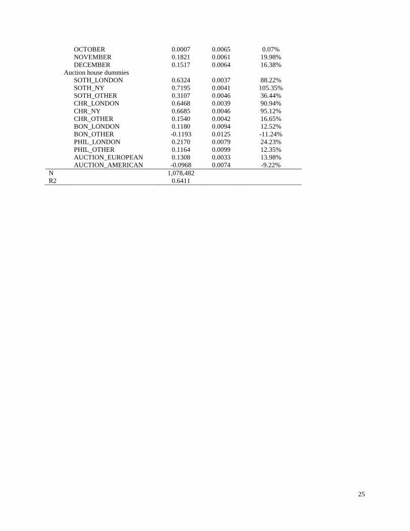
Table 2 – Baseline hedonic regression results Table 2 presents the baseline hedonic regression results. Eq. (1) is estimated using OLS. The dependent variable is the natural log of the price in year 2007 USD. The descriptive statistics for the independent variables are shown in Table 1. For each variable, we report the coefficient (β), the standard deviation (S.D.), and the price impact (i.e., the exponent of the coefficient minus one). The number of observations (N) and the R-squared (R2) are presented at the bottom of the table. β S.D. exp(β) - 1

Year dummies [included] Artist characteristics Artist dummies [included] TEXTBOOK 0.1263 0.0065 13.46% Work characteristics Attribution dummies ATTRIBUTED -0.7365 0.0050 -52.12%

STUDIO -0.7977 0.0134 -54.96%

CIRCLE -1.0490 0.0068 -64.97%

SCHOOL -1.4152 0.0120 -75.71%

AFTER -1.8850 0.0104 -84.82%

STYLE -1.5688 0.0064 -79.17%

Authenticity dummies SIGNED 0.2703 0.0027 31.04%

DATED 0.1706 0.0026 18.60%

Medium dummies OIL [left out] WATERCOLOR -0.7144 0.0033 -51.05%

DRAWING -1.1005 0.0030 -66.73%

Size variables HEIGHT 0.0205 0.0002 2.07%

WIDTH 0.0250 0.0002 2.53%

HEIGHT_2 -0.0001 0.0000 -0.01%

WIDTH_2 -0.0001 0.0000 -0.01%

Topic dummies STUDY -0.2049 0.0078 -18.53%

ABSTRACT -0.0780 0.0068 -7.50%

ANIMALS -0.1703 0.0094 -15.66%

LANDSCAPE -0.1320 0.0048 -12.37%

NUDE -0.1645 0.0105 -15.17%

PEOPLE -0.0372 0.0050 -3.65%

PORTRAIT -0.2278 0.0050 -20.37%

RELIGION -0.1114 0.0082 -10.54%

SELF-PORTRAIT 0.1202 0.0171 12.77%

STILL_LIFE 0.0410 0.0067 4.18%

UNTITLED -0.1639 0.0065 -15.12%

URBAN 0.0409 0.0081 4.17% Sale characteristics Month dummies JANUARY [left out] FEBRUARY -0.1209 0.0072 -11.39%

MARCH 0.0318 0.0065 3.23%

APRIL 0.0859 0.0065 8.97%

MAY 0.1325 0.0062 14.16%

JUNE 0.1430 0.0063 15.37%

JULY 0.0843 0.0070 8.80%

AUGUST -0.0629 0.0101 -6.09%

SEPTEMBER -0.1599 0.0077 -14.78%

25

OCTOBER 0.0007 0.0065 0.07%

NOVEMBER 0.1821 0.0061 19.98%

DECEMBER 0.1517 0.0064 16.38%

Auction house dummies SOTH_LONDON 0.6324 0.0037 88.22%

SOTH_NY 0.7195 0.0041 105.35%

SOTH_OTHER 0.3107 0.0046 36.44%

CHR_LONDON 0.6468 0.0039 90.94%

CHR_NY 0.6685 0.0046 95.12%

CHR_OTHER 0.1540 0.0042 16.65%

BON_LONDON 0.1180 0.0094 12.52%

BON_OTHER -0.1193 0.0125 -11.24%

PHIL_LONDON 0.2170 0.0079 24.23%

PHIL_OTHER 0.1164 0.0099 12.35%

AUCTION_EUROPEAN 0.1308 0.0033 13.98% AUCTION_AMERICAN -0.0968 0.0074 -9.22% N 1,078,482 R2 0.6411

26

Table 3 – Baseline art price indices and art returns Table 3 presents the art price indices and returns for the baseline hedonic regression model detailed in Table 2. For each year, we report the dummy coefficient (γ), the standard deviation (S.D.), the variance of the residuals (σ2), the uncorrected price index and return (Π and r), and the price index and return that are corrected for changes in price dispersion over time (Π* and r*) (cf. Section III). Index values for 1963 are geometrically interpolated. Year γ S.D. σ2 Π r Π* r* 1957

1.1789 100.00

100.00

1958 -0.0817 0.0402 1.1144 92.16 -7.84% 89.23 -10.77% 1959 0.2102 0.0384 1.2183 123.39 33.89% 125.85 41.03% 1960 0.2275 0.0380 1.1131 125.55 1.75% 121.48 -3.47% 1961 0.3014 0.0382 1.1805 135.18 7.67% 135.28 11.36% 1962 0.3327 0.0353 1.1744 139.47 3.18% 139.16 2.86% 1963 - - - 140.72 0.89% 140.61 1.04% 1964 0.3505 0.0355 1.1803 141.97 0.89% 142.07 1.04% 1965 0.5273 0.0338 1.1770 169.44 19.35% 169.27 19.15% 1966 0.6390 0.0345 0.9487 189.45 11.81% 168.85 -0.25% 1967 0.7044 0.0347 0.9466 202.26 6.76% 180.07 6.65% 1968 0.8423 0.0334 1.0564 232.17 14.79% 218.37 21.27% 1969 0.8716 0.0335 1.0208 239.08 2.98% 220.90 1.16% 1970 0.7773 0.0325 0.9335 217.57 -9.00% 192.44 -12.88% 1971 0.9410 0.0312 0.9100 256.25 17.78% 224.01 16.40% 1972 1.1224 0.0308 1.0856 307.22 19.89% 293.22 30.89% 1973 1.3932 0.0304 0.9249 402.77 31.10% 354.73 20.98% 1974 1.2909 0.0303 0.9030 363.61 -9.72% 316.75 -10.71% 1975 1.0670 0.0304 0.8847 290.66 -20.06% 250.89 -20.79% 1976 0.9606 0.0301 0.8685 261.31 -10.10% 223.75 -10.82% 1977 0.9581 0.0300 0.8779 260.68 -0.24% 224.25 0.22% 1978 1.0943 0.0300 0.8710 298.69 14.58% 256.07 14.19% 1979 1.1720 0.0299 0.8397 322.86 8.09% 272.49 6.41% 1980 1.1763 0.0299 0.8148 324.22 0.42% 270.26 -0.82% 1981 1.0436 0.0299 0.8329 283.94 -12.43% 238.83 -11.63% 1982 0.8652 0.0300 0.8095 237.56 -16.34% 197.49 -17.31% 1983 0.8888 0.0299 0.8137 243.21 2.38% 202.62 2.60% 1984 0.9058 0.0298 0.8711 247.40 1.72% 212.10 4.68% 1985 0.9976 0.0298 0.8566 271.17 9.61% 230.80 8.82% 1986 1.2319 0.0298 0.8567 342.76 26.40% 291.75 26.40% 1987 1.5505 0.0297 0.8845 471.38 37.53% 406.86 39.46% 1988 1.7498 0.0297 0.8662 575.35 22.06% 492.07 20.94% 1989 1.9651 0.0296 0.9220 713.58 24.03% 627.57 27.54% 1990 2.0252 0.0297 0.9227 757.79 6.20% 666.68 6.23% 1991 1.6356 0.0298 0.7791 513.24 -32.27% 420.25 -36.96% 1992 1.5304 0.0298 0.7576 462.02 -9.98% 374.26 -10.95% 1993 1.3661 0.0298 0.7699 392.01 -15.15% 319.51 -14.63% 1994 1.3595 0.0297 0.8066 389.41 -0.66% 323.27 1.18% 1995 1.3727 0.0297 0.8103 394.58 1.33% 328.17 1.52% 1996 1.3678 0.0297 0.7994 392.66 -0.49% 324.78 -1.03% 1997 1.3676 0.0297 0.8437 392.60 -0.02% 332.02 2.23% 1998 1.3954 0.0297 0.8626 403.65 2.82% 344.60 3.79% 1999 1.4458 0.0297 0.8745 424.54 5.17% 364.60 5.80% 2000 1.4157 0.0297 0.9165 411.94 -2.97% 361.28 -0.91% 2001 1.3539 0.0297 0.9354 387.26 -5.99% 342.86 -5.10% 2002 1.4276 0.0297 0.9354 416.88 7.65% 369.08 7.65% 2003 1.5405 0.0297 0.8974 466.69 11.95% 405.40 9.84% 2004 1.6462 0.0297 0.9214 518.74 11.15% 456.07 12.50% 2005 1.6691 0.0296 0.9769 530.76 2.32% 479.76 5.19% 2006 1.7724 0.0296 1.0711 588.51 10.88% 557.62 16.23% 2007 1.9786 0.0299 1.1133 723.27 22.90% 699.91 25.52%

27

Table 4 – Annualized returns for baseline indices, robustness checks, and extensions Panel A of Table 4 presents the annualized (i.e., geometric average) returns and standard deviations (S.D.) over the periods 1957-2007 and 1982-2007 for the baseline art price indices detailed in Table 3. It also shows the number of observations (N) included in the estimation. Panel B shows the results for a number of robustness checks (cf. Section IV.B). Panel C repeats the adjacent-period hedonic model using quantile regressions (cf. Section IV.C). Panel D presents the RSR results for two different trading strategies (cf. Section IV.D). Panel E shows the return estimates (corrected for changes in price dispersion over time) for the different mediums and movements considered in this study (cf. Section IV.E).

N Real returns

1957-2007

1982-2007

Mean S.D. Mean S.D. Panel A: Baseline indices

Art price index Π 1,078,482

4.04% 16.68%

4.55% 14.39%

Art price index Π* 1,078,482

3.97% 15.21%

5.19% 15.31%

Panel B: Robustness checks (compare to Π)

Drop topic dummies 1,078,482

4.02% 14.05%

4.53% 14.39%

Exclude artists < 100 sales 935,736

4.04% 14.26%

4.57% 14.69%

Exclude Min. & Cont. 1,059,010

4.00% 13.95%

4.48% 14.26%

Adjacent-period model -

- -

4.60% 13.62%

Repeat-sales regression (RSR) 21,846 (x2)

- -

4.56% 15.79%

Panel C: Quantile regressions

Q95 862,290

- -

6.32% 18.99%

Q75 862,290

- -

5.77% 16.54%

Q50 862,290

- -

4.91% 15.11%

Q25 862,290

- -

3.89% 13.84%

Q05 862,290

- -

1.35% 12.57%

Panel D: Trading strategies (compare to RSR)

“Masterpiece” strategy 1,467 (x2)

- -

4.81% 22.08%

“Value” strategy 727 (x2)

- -

6.16% 20.99%

Panel E: Indices per medium and per movement

Oil 650,563

4.63% 14.69%

5.73% 15.39%

Watercolor 187,612

3.67% 16.38%

3.96% 14.79%

Drawing 240,307

2.51% 20.64%

4.37% 15.22%

Medieval & Renaissance 30,806

3.01% 27.13%

6.44% 19.59%

Baroque 124,617

4.76% 17.69%

5.82% 12.57%

Rococo 30,292

3.69% 25.42%

5.03% 12.15%

Neoclassicism 12,601

6.32% 45.93%

5.36% 22.45%

Romanticism 41,897

4.28% 17.34%

4.79% 15.24%

Realism 60,820

2.57% 21.42%

4.16% 15.46%

Impressionism & Symbolism 95,829

4.10% 24.01%

4.55% 16.70%

Fauvism & Expressionism 73,543

3.72% 22.84%

4.90% 18.36%

Cubism, Futurism & Constr. 49,056

5.53% 22.40%

6.01% 20.55%

Dada & Surrealism 49,697

5.85% 32.32%

5.58% 19.42%

Abstract Expressionism 35,960

- -

7.78% 21.91%

Pop 18,924

- -

10.35% 29.33%

Minimalism & Contemporary 19,472 - - 7.07% 23.68%

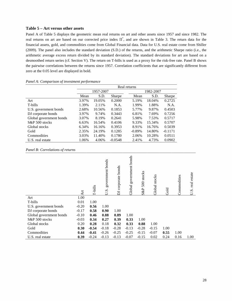
28

Table 5 – Art versus other assets Panel A of Table 5 displays the geometric mean real returns on art and other assets since 1957 and since 1982. The real returns on art are based on our corrected price index Π*, and are shown in Table 3. The return data for the financial assets, gold, and commodities come from Global Financial data. Data for U.S. real estate come from Shiller (2009). The panel also includes the standard deviation (S.D.) of the returns, and the arithmetic Sharpe ratio (i.e., the arithmetic average excess return divided by its standard deviation). The standard deviations for art are based on a desmoothed return series (cf. Section V). The return on T-bills is used as a proxy for the risk-free rate. Panel B shows the pairwise correlations between the returns since 1957. Correlation coefficients that are significantly different from zero at the 0.05 level are displayed in bold. Panel A: Comparison of investment performance

Real returns

1957-2007

1982-2007

Mean S.D. Sharpe Mean S.D. Sharpe Art 3.97% 19.05% 0.2000 5.19% 18.04% 0.2725 T-bills 1.39% 2.11% N.A.

1.99% 1.88% N.A.

U.S. government bonds 2.68% 10.56% 0.1853

5.77% 9.87% 0.4503 DJ corporate bonds 3.97% 9.74% 0.3443

6.81% 7.69% 0.7256

Global government bonds 3.07% 8.19% 0.2641

5.98% 7.53% 0.5717 S&P 500 stocks 6.63% 16.54% 0.4106

9.33% 15.34% 0.5707

Global stocks 6.34% 16.16% 0.3953

8.91% 16.76% 0.5039 Gold 2.35% 24.19% 0.1285

-0.89% 14.80% -0.1171

Commodities 3.03% 11.40% 0.1780

2.06% 10.28% 0.0511 U.S. real estate 1.06% 4.06% -0.0548 2.41% 4.73% 0.0902

Panel B: Correlations of returns

Art

T-bi

lls

U.S

. gov

ernm

ent b

onds

DJ c

orpo

rate

bon

ds

Glo

bal g

over

nmen

t bon

ds

S&P

500

stoc

ks

Glo

bal s

tock

s

Gol

d

Com

mod

ities

U.S

. rea

l est

ate

Art 1.00 T-bills 0.01 1.00

U.S. government bonds -0.20 0.56 1.00 DJ corporate bonds -0.17 0.58 0.90 1.00

Global government bonds -0.10 0.46 0.88 0.89 1.00 S&P 500 stocks -0.03 0.34 0.27 0.39 0.33 1.00

Global stocks 0.20 0.28 0.18 0.32 0.33 0.88 1.00 Gold 0.30 -0.54 -0.18 -0.28 -0.13 -0.28 -0.15 1.00

Commodities 0.44 -0.41 -0.26 -0.25 -0.25 -0.15 -0.07 0.55 1.00 U.S. real estate 0.39 -0.24 -0.13 -0.13 -0.07 -0.15 0.02 0.24 0.16 1.00

29

Table 6 – Explaining the returns on art Table 6 presents the results of a linear regression of art returns on a number of independent variables, over the period 1981-2007. Below each coefficient, we report Newey-West standard errors that control for heteroskedasticity and autocorrelation up to two lags. The real returns on art are based on our corrected price index Π*, and are shown in Table 3. Model (1) only includes same-year and lagged global stock returns, from Global Financial Data, as independent variables. Column (2) adds (lagged and standardized) data from the University of Michigan’s Survey of Consumers on the attitude of high-income (upper third) consumers with respect to the purchase of “major household items”. Model (3) adds a newly constructed (lagged and standardized) art market sentiment measure, based on volume and buy-in rates at high-profile auctions, and on media reports (cf. Section VI). The number of observations (N) and the adjusted R-squared (R2) are presented at the bottom of the table.

(1)

(2)

(3)

Dependent variable: real returns on art

Same-year global stock returns 0.1751

0.1325

0.1184

(0.1050)

(0.0901)

(0.0987)

Previous-year global stock returns 0.5396 ** 0.4012 * 0.2976

(0.2534)

(0.1941)

(0.2066)

High-income consumer confidence

0.0677 *** 0.0554 **

(0.0226)

(0.0231)

Art market sentiment

0.0425 **

(0.0175)

N 27

27

27

Adjusted R2 0.33 0.49 0.52

30

Figure 1 – Hedonic price indices Figure 1 presents the baseline art price indices detailed in Table 3. Π is the uncorrected price index, while Π* corrects for changes in price dispersion over time. The figure also includes the average and median real price for each year in our data set.

Figure 2 – Quantile regressions Figure 2 presents the art price indices that result from repeating the adjacent-period hedonic model using quantile regressions (cf. Section IV.C).

0

100

200

300

400

500

600

700

800

1957

1959

1961

1963

1965

1967

1969

1971

1973

1975

1977

1979

1981

1983

1985

1987

1989

1991

1993

1995

1997

1999

2001

2003

2005

2007

Π (uncorrected) Π* (corrected)

Average real price Median real price

0

50

100

150

200

250

300

350

400

450

500

1982

1983

1984

1985

1986

1987

1988

1989

1990

1991

1992

1993

1994

1995

1996

1997

1998

1999

2000

2001

2002

2003

2004

2005

2006

2007

Q95 Q75 Q50 Q25 Q05

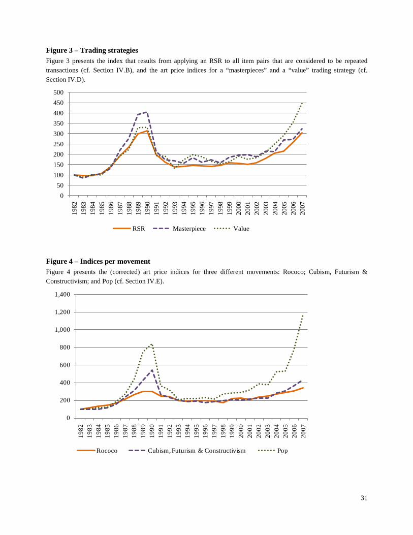
31

Figure 3 – Trading strategies Figure 3 presents the index that results from applying an RSR to all item pairs that are considered to be repeated transactions (cf. Section IV.B), and the art price indices for a “masterpieces” and a “value” trading strategy (cf. Section IV.D).

Figure 4 – Indices per movement Figure 4 presents the (corrected) art price indices for three different movements: Rococo; Cubism, Futurism & Constructivism; and Pop (cf. Section IV.E).

050

100150200250300350400450500

1982

1983

1984

1985

1986

1987

1988

1989

1990

1991

1992

1993

1994

1995

1996

1997

1998

1999

2000

2001

2002

2003

2004

2005

2006

2007

RSR Masterpiece Value

0

200

400

600

800

1,000

1,200

1,400

1982

1983

1984

1985

1986

1987

1988

1989

1990

1991

1992

1993

1994

1995

1996

1997

1998

1999

2000

2001

2002

2003

2004

2005

2006

2007

Rococo Cubism, Futurism & Constructivism Pop

32

Figure 5 – Art market sentiment Figure 5 presents the end-of-year values for the art market sentiment measure used in this study. It is based on volume and buy-in rates at high-profile auctions, and on media reports (cf. Section VI). It is standardized to have zero mean and unit variance.

-3

-2

-1

0

1

2

3

1980

1981

1982

1983

1984

1985

1986

1987

1988

1989

1990

1991

1992

1993

1994

1995

1996

1997

1998

1999

2000

2001

2002

2003

2004

2005

2006