This article was downloaded by: [Universite De Paris 1]On: 19 May 2013, At: 09:10Publisher: RoutledgeInforma Ltd Registered in England and Wales Registered Number: 1072954 Registered office: MortimerHouse, 37-41 Mortimer Street, London W1T 3JH, UK

Quantitative FinancePublication details, including instructions for authors and subscription information:http://www.tandfonline.com/loi/rquf20

Buyer's quantile hedge portfolios in discrete-timetradingMustafa Ç. Pinar aa Department of Industrial Engineering , Bilkent University , Ankara 06800 , TurkeyPublished online: 22 Mar 2011.

To cite this article: Mustafa Ç. Pinar (2013): Buyer's quantile hedge portfolios in discrete-time trading, QuantitativeFinance, 13:5, 729-738

To link to this article: http://dx.doi.org/10.1080/14697688.2010.538075

PLEASE SCROLL DOWN FOR ARTICLE

Full terms and conditions of use: http://www.tandfonline.com/page/terms-and-conditions

This article may be used for research, teaching, and private study purposes. Any substantial or systematicreproduction, redistribution, reselling, loan, sub-licensing, systematic supply, or distribution in any form toanyone is expressly forbidden.

The publisher does not give any warranty express or implied or make any representation that the contentswill be complete or accurate or up to date. The accuracy of any instructions, formulae, and drug dosesshould be independently verified with primary sources. The publisher shall not be liable for any loss, actions,claims, proceedings, demand, or costs or damages whatsoever or howsoever caused arising directly orindirectly in connection with or arising out of the use of this material.

Quantitative Finance, 2013

Buyer’s quantile hedge portfolios in

discrete-time trading

MUSTAFA C. PINAR*

Department of Industrial Engineering, Bilkent University, Ankara 06800, Turkey

(Received 21 April 2009; in final form 29 October 2010)

The problem of quantile hedging for American claims is studied from the perspective of thebuyer of a contingent claim by minimizing the ‘expected failure ratio’. After a general study ofthe problem in infinite-state spaces, we pass to finite dimensions and examine the properties ofthe resulting finite-dimensional optimization problems. In finite-state probability spaces weobtain a bilinear programming formulation that admits an exact linearization using binaryexercise variables. Numerical results with S&P 500 index options demonstrate the compu-tational viability of the formulations.

Keywords: Asset pricing; Optimization; Risk management; American style derivative securities

1. Introduction

A fundamental problem of financial economics is thepricing of financial instruments called ‘contingent claims’.When an arbitrage-free financial market is not complete,it is well-known that there exists a set of ‘risk-neutral’probability measures that make the (discounted) prices oftraded instruments martingales. An important feature ofthe set of risk-neutral measures is that the value of thecheapest portfolio to dominate the pay-off at maturity ofa contingent claim coincides with the maximum expectedvalue of the (discounted) pay-off of the claim with respectto this set. This value, called the ‘super-hedging price’,allows the seller to assemble a portfolio that achieves avalue at least as large as the pay-off to the claim holder atthe maturity date of the claim in all non-negligible events.By a similar reasoning, the largest price that a potentialbuyer is willing to disburse to acquire a contingent claimis called a ‘sub-hedging price’ (or lower hedging price),which is equal to the value of the most precious portfoliothat is dominated by the contingent claim pay-off atmaturity. (If the claim is attainable, then the smallest priceto super-hedge and the largest price to sub-hedge areequal to the hedging price, and the expected value doesnot depend on the chosen risk-neutral measure, so theprevious statement still applies.) The super-hedging priceis the natural price to be asked by the writer of acontingent claim and, together with the bid price obtained

by considering the analogous problem from the point of

view of the buyer, it constitutes an interval that is

sometimes called the ‘no-arbitrage price interval’ for the

claim in question.A writer may not always ask for the whole

super-hedging price to ‘sell’ a claim with pay-off FT

(see, e.g., Follmer and Schied 2004, chapters 7 and 8 for a

discussion and examples showing that the super-hedging

price may be too high). On the other hand, some

economic considerations such as pre-existing endowments

or liabilities may induce a buyer to pay a larger price than

the sub-hedging price to acquire the claim. It may also be

the case that the no-arbitrage buyer price, i.e. the

sub-hedging price, may be too low to be interesting for

any potential seller. In such a case, neither buyer nor

seller will be able to set up sub-hedging or super-hedging

portfolios, which implies that they will face a positive

probability of ‘falling short’, i.e. for the writer his/her

portfolio will take values VT smaller than those of the

claim on a non-negligible event, and for the buyer his/her

portfolio will take values VT larger than those of the claim

on a non-negligible event. Thus, the writer and the buyer

will need to choose hedging strategies according to some

optimality criterion to be decided. One such criterion that

has been widely studied comes from the idea of quantile

hedging, which consists of choosing a hedge portfolio that

minimizes the probability of a shortfall in the case of a

writer. The problem has been studied in several papers

(Spivak and Cvitanic 1999, Follmer and Leukert 2000,

Nakano 2003, 2004, Rudloff 2007, 2009) in discrete time*Email: mustafap@bilkent.edu.tr

Vol. 13, No. http://dx.doi.org/10.1080/14697688.2010.5380755, 729–738,

� 201 Taylor & Francis3

Dow

nloa

ded

by [

Uni

vers

ite D

e Pa

ris

1] a

t 09:

10 1

9 M

ay 2

013

and infinite state spaces or in continuous time, almostexclusively—to the best of this author’s knowledge—fromthe viewpoint of a writer of a European claim.Perez-Hernandez (2007) studied the problem of quantilehedging for American contingent claims in an infinite-state space setting from the perspective of the writer of theclaim.

The purpose of this paper is to study quantile hedgingportfolio strategies from a buyer’s perspective underdiscrete-time trading in incomplete markets for Americanclaims. We analyse the problem both in infinite- andfinite-state spaces. In the latter case, we formulate theassociated optimization problems as problems that can betreated numerically by available software, and investigatetheir properties. The resulting bilinear programmingformulations for lower quantile hedging of Americancontingent claims are new, and appear for the first time inthe present paper, to the best of the author’s knowledge.

The rest of the paper is organized as follows. In section2 we recall briefly the quantile hedge problem from awriter’s point of view. Section 3 is devoted to the quantilehedge problems of American contingent claims in general,and section 4 to the same problems in finite-dimensionalspaces, from a buyer’s perspective. An interesting aux-iliary—but important in its own right—result allows us toobtain a compact, bilinear, continuous optimizationformulation. Using the binary nature of variables thatrepresent exercise strategies for the American claim, weobtain a linear mixed-integer programming formulationthat is equivalent to the bilinear continuous formulation.Finally, section 5 is devoted to the numerical testing of theformulations of the paper using data from S&P 500options. It appears that the linearized version of thebilinear formulation, while giving rise to large optimiza-tion problems, may be processed numerically by availablesoftware.

A common criticism leveled against the criterion ofquantile hedging is that it ignores the magnitude of thelosses (Follmer and Schied 2004). In response to thiscriticism, several authors have studied the criterion ofexpected shortfall minimization (see, e.g., Nakano (2003),Follmer and Schied (2004) and Rudloff (2007, 2009)).We will investigate this criterion in the spirit of thepresent paper, that is, from a buyer’s perspective, in asubsequent work.

2. Background on writer’s quantile hedge for

European claims

In the present paper, we work in a financial marketM¼ (�,F ,P,T,S, {F t}t2T) with discrete-time tradingover the time set T¼ {0, 1, . . . ,T } and where(�,F ,P, {F}t2T) is a complete filtered probability space,and S¼ {St}t2T is an R

2þ asset price process over the time

set T adapted to the filtration {F}t2T. We assume withoutloss of generality that the first component of S is thenumeraire security, i.e. S0

t ¼ 1 for all t2T. Let Q be theset of equivalent martingale measures in the arbitrage-free

(not necessarily complete) marketM. For the rest of the

paper we make the following blanket assumption.

Assumption 2.1: The market is arbitrage free, i.e. the set

Q is non-empty.

Let us recall the problem of quantile hedging from the

point of view of the writer of a contingent claim. The

problem in the form that we will address was studied by

Follmer and Leukert (2000). The idea is the following. Fix

a capital v smaller than the no-arbitrage price for the

contingent claim H with (discounted with respect to the

numeraire) pay-offs {Ht}t2T, i.e. v5�"(H )� supQ2Q

EQ[HT], and find a hedge policy that maximizes the

probability of success, where the probability of success is

the probability of the event that the value of an admissible

portfolio strategy at the time of expiration of the claim is

at least as large as the value of the claim. A self-financing

trading strategy is called admissible if its value process is

non-negative at the time of expiration of the contingent

claim (Follmer and Schied 2004, definition 8.1). Hence,

the problem is to construct an admissible strategy ��� suchthat its value process V� satisfies

P½V�T � H� ¼ maxP½VT � H�, ð1Þ

where the maximum is searched for in the set of all

admissible portfolio strategies satisfying

V0 � v: ð2Þ

The set {VT�H} is termed the success set. Follmer and

Schied (2004) show that the problem is guaranteed to

admit a closed-form solution for complete markets, under

a technical condition that may not always be verified

(Follmer and Leukert 2000). More precisely, let Q be a

singleton, i.e. Q¼ {Q�}. Assuming that A� maximizes the

probability P[A] among all sets A2FT satisfying the

constraint

EQ�

½H11A� � v,

the replicating strategy ��� of the knock-out option

H� ¼ H11A� solves the above optimization problem. To

construct the optimal set A� using the Neyman–Pearson

theory, an auxiliary measure Q� is introduced, given by

dQ�

dQ� ¼

H

EQ�

½H�:

The set A� was explicitly pointed out by Follmer and

Schied (2004, chapter 8). If

Q�½A�� ¼v

EQ�

½H�,

then A� maximizes P[A] among all sets A2FT satisfying

the constraint

EQ�

½H11A� � v,

and the replicating strategy of H11A� solves the prob-

lem (1)–(2). However, in general it may be impossible to

find such a set A� with probability under Q� exactly equal

to v=EQ�

½H�. Hence, Follmer and Leukert introduced

2 M.C. Pinar730

Dow

nloa

ded

by [

Uni

vers

ite D

e Pa

ris

1] a

t 09:

10 1

9 M

ay 2

013

an extended version of the problem where the so-called‘expected success ratio’ is minimized.

For an admissible strategy � and its value process V wedefine the success ratio V of � by

V :¼ 11fVT�Hg þVT

H11fVT5Hg ¼

VT

H^ 1:

For an amount v5�"(H ), the writer’s problem consistsof searching among all admissible strategies, with initial

endowment equal to at most v, for one that maximizes theexpected success ratio. In other words, the problem ofinterest to the writer is problem [WECP] over variables �that are admissible adapted portfolio strategies � (and

their value processes V )

sup

s:t:

EP½ V�,

V0 � v:

The set { V¼ 1} coincides with the success set

{VT�H} of V. Instead of solving the above problem,Follmer and Leukert (2000) and Follmer and Schied(2004) advocate solving the auxiliary problem

sup EP½ �,

s:t: supQ2Q

EQ½H � � v,

2 ½0, 1� P-a.s.

They show that a solution � exists and the valueprocess of a super-hedging strategy for the modified claimH � leads to the optimal success set corresponding toinitial capital v. The details can be found in Follmer and

Schied (2004, chapter 8). The above ideas were extendedto the case of American contingent claims from theviewpoint of the writer by Perez-Hernandez (2007).

3. Quantile hedging: Buyer’s view for American claims

The study of American contingent claims poses an

additional challenge due to the presence of the earlyexercise possibility. For an in-depth treatment ofAmerican contingent claims in discrete time, our desktop

reference is Follmer and Schied (2004). One common wayto describe exercise strategies of American claims is bystopping times. These are functions � :

�! {0, . . . ,T}[ {þ1} such that {!2� | �(!)¼ t}2F t,for each t¼ 0, . . . ,T. Let T denote the set of stoppingtimes. It is well-known that the buyer lower hedging priceof an American claim with pay-off process C¼ {Ct}t2T is

given by

�#ðCÞ ¼ sup�2T

infQ2Q

EQ½C��:

We shall refer to �#(C) as the sub-hedging price forAmerican claim C. Chalasani and Jha (2001) show that

�#(C) can be obtained as the optimal value of thefollowing optimization problem:

max�2�f�V0ð�Þ j 9� 2 T s.t. V�ð�Þ þ C� � 0g,

where � represents the set of self-financing portfolio

strategies �. Assuming �� is an optimal portfolio strategy

and �� an optimal exercise rule, the buyer borrows the

amount V0(��) at time 0 to pay the seller for the

contingent claim, and acquires the claim. At the time ��

of exercise of the claim, the buyer repays his/her debt

incurred at time 0. We refer to the optimal portfolio

strategy of the buyer as a ‘sub-hedging strategy’. A sub-

hedging strategy �� has the property that Vt(��)�Ct on

{Ct40} for all t2T, and VT� 0 (Chalasani and Jha 2001,

Follmer and Schied 2004, Pennanen and King 2006).Following Perez-Hernandez (2007), let the American

contingent claim C¼ {Ct}t2T be a given non-negative

adapted and P-integrable process. For a portfolio strat-

egy � we define the ‘failure ratio’ process � of � by

�t :¼ 11fVtð�Þ�Ctg þVtð�Þ

Ct11fVtð�Þ4Ctg ¼

Vtð�Þ

Ct_ 1:

For an amount v4�#(C ), the buyer’s problem consists of

searching among all self-financing portfolio strategies,

with initial endowment equal to at least v, for one that

minimizes the maximum of the expected failure ratio over

all stopping times. In other words, the problem of interest

to the buyer is problem ACP (American Claim Problem)

inf sup�2T

EP½ �� �,

s:t: V0ð�Þ�v:

We define by R the set of [1, 1]-valued adapted

processes, i.e.

R¼f ¼f tgt2T : t 2 ½1,1�, andF t-measurable, 8t2Tg:

For the American claim C we define the subset R0 of R

R0 ¼ 2 R : infQ2Q

sup�2T

EQ½C� � � � v

� �:

We are interested in solving the problem [PACP] as a

proxy to [ACP]

inf sup�2T

EP½ � �,

s:t: infQ2Q

sup�2T

EQ½C� � � � v,

2 ½1,1� P-a.s.

As an elementary observation note that, if t solves

[PACP], every process � 2 R0 with � t � t, 8t2T, also

solves [PACP].

Theorem 3.1: Let the infimum in PACP be finite. Then we

have the following.

(1) The problem [PACP] has an optimal solution, i.e.

there exists a 2 R0 with

sup�2T

EP½ �� ¼ min

2R0

sup�2T

EP½ � �

� �:

(2) For an optimal solution of [PACP], a sub-hedging

strategy � for the adjusted American claim

C ¼ C � is a solution of problem ACP.

Buyer’s quantile hedge portfolios in discrete-time trading 3731

Dow

nloa

ded

by [

Uni

vers

ite D

e Pa

ris

1] a

t 09:

10 1

9 M

ay 2

013

Proof: For part 1, observe that in [PACP] the functional

f ð Þ � EP½ �� is a linear functional in � for fixed �. Since

the supremum of an arbitrary collection of linear func-

tionals is convex and piecewise linear (Van Tiel 1984), the

objective function in [PACP] is a convex functional in .Now fix �4 inf 2R0

f . Since the level set lev( f, �)¼ { |

f ( )� �} is convex, and closed (Van Tiel 1984), the set

lev( f, �)\ { | 2 [1,1] P-a.s.} is closed and bounded,

and hence compact using the assumption that

inf 2R0f4�1. On the other hand, the set { | infQ2Q

sup�2T EQ[C� �]� v} is closed, hence its intersection with

lev( f, �)\ { | 2 [1,1] P-a.s.} is a compact set. Since

PACP is equivalent to minimizing f over lev( f, �)\ { |

2 [1,1] P-a.s.}\ { | infQ2Q sup�2T EQ[C� �]� v}, a

compact set by the previous assertion, f attains its

infimum over this set by the Weierstrass’ theorem. This

proves part 1.For part 2, let � be a self-financing portfolio strategy

with V0(�)� v and VT� 0, and � 2T be a stopping time.

Using Doob’s Stopping Theorem (Follmer and Schied

2004, theorem 6.17) on the Q-martingale V(�) we

have that

EQ½C�

��� ¼ E

Q½V�ð�Þ _ C�� � E

Q½V0ð�Þ� � v,

hence �2R0, and as a feasible point of [ACFP] we obtain

sup�2T

EP½ ��� � sup

�2TE

P½ ��: ð3Þ

Now let us consider a sub-hedging strategy � for the

adjusted American claim C � C . Using the correspond-

ing failure ratio � we have

Ct � �t ¼ Ct _ Vtð�Þ � Ct _ ðCt Þ ¼ Ct :

Therefore, �t is dominated by t on the set {Ct40}.

Moreover, any failure ratio is equal to 1 on {Ct¼ 0}

following a reasoning similar to Perez-Hernandez (2007).

Hence, we obtain

�t � t, P-a.s.

Now, since every process � such that � t � t for all t2T

is also a solution to PACP we obtain that � solves [PACP].

Combined with (3), we have that sup�2T EP½ ��� ¼

sup�2T EP½ � � and � solves [ACP]. h

For an optimal �, the sub-hedging portfolio strategy

for the scaled-up claim C � is the optimal quantile hedge

strategy corresponding to initial capital v. We nextinvestigate the ramifications of this result in finite-state

markets.

4. Buyer’s problem for American claims in finite-state

markets

In finite-state markets, we can transform PACP into a

finite-dimensional optimization problem that can be

processed numerically by existing optimization algo-rithms and software.

4.1. The finite-state market

Now we assume � has a finite number of atoms, i.e.�¼ {!1, . . . ,!K}. More precisely, we assume as in King(2002) that security prices and other payments are discreterandom variables supported on a finite probability space(�,F ,P) whose atoms are sequences of real-valuedvectors (asset values) over discrete time periodst2T¼ {0, 1, . . . ,T}. The market evolves as a discrete,non-recombinant scenario tree in which the partition ofprobability atoms !2� generated by matching pathhistories up to time t corresponds one-to-one with nodesn2N t at level t in the tree. The set N 0 consists of the rootnode n¼ 0, and the leaf nodes n2N T correspond one-to-one with the probability atoms !2�. While not needed inthe finite probability setting, the �-algebras F t generatedby the partitions N t are such that F 0¼ {;, �}, F tF tþ1

for all 0� t�T� 1 and FT¼F . A stochastic process issaid to be ðF tÞ

Tt¼0-adapted if, for each t¼ 0, . . . ,T, the

outcome of the process only depends on the element of F t

that has been realized at stage t. Similarly, a decisionprocess is said to be ðF tÞ

Tt¼0-adapted if, for each t2T, the

decision depends on the element of F t that has beenrealized at stage t. In the scenario tree, every node n2N t

for t¼ 1, . . . ,T has a unique parent denoted �(n)2N t�1,and every node n2N t, t¼ 0, 1, . . . ,T� 1, has a non-empty set of child nodes C(n)N tþ1. We denote the set ofall nodes in the tree by N . The set A(n) denotes thecollection of ascendant nodes or the unique path leadingto node n (including itself) from node 0 and the set D(n)denotes the collection of descendant nodes of node nincluding itself. The probability distribution P is obtainedby attaching positive weights pn to each leaf node n2N T

so thatP

n2N Tpn ¼ 1. For each non-leaf (intermediate

level) node in the tree, i.e. for all ‘2N nN T, theprobability is determined recursively by

p‘ ¼X

m2CðnÞ

pm, 8n 2 N t, t ¼ T� 1, . . . , 0:

Hence, each non-leaf node has a probability mass equal tothe combined mass of its child nodes.

A stochastic process {Xt} is a time-indexed collection ofrandom variables such that each Xt is a random variablewith realizations Xn for all n2N t. The expected value ofXt is uniquely defined by the sum

EP½Xt� :¼

Xn2N t

pnXn:

The conditional expectation of Xtþ1 on N t is given by theexpression

EP½Xtþ1 j N t� :¼

Xm2CðnÞ

pmpn

Xm:

The market consists, as in the previous section, of a bondand a single risky security with prices at node n given by

4 M.C. Pinar732

Dow

nloa

ded

by [

Uni

vers

ite D

e Pa

ris

1] a

t 09:

10 1

9 M

ay 2

013

the two-dimensional vector Sn ¼ ðS0n,S

1nÞ

T. The number ofshares of securities held by the investor in state (node)n2N t is denoted �n2R

2. Therefore, to each state n2N t

is associated the two-dimensional real vector �n. The valueof the portfolio at state n is Sn � �n. We assume withoutloss of generality that prices at all nodes have been scaledso that S0

n ¼ 1 for all n2N . The assumption of a singlerisky security can easily be relaxed, and the developmentof the paper can be repeated for multiple securities,mutatis mutandis.

Definition 4.1: If there exists a probability measureQ ¼ fqngn2NT such that

St ¼ EQ½Stþ1 j N t� ðt � T� 1Þ,

then the process {St} is called a martingale under Q, andQ is called a martingale probability measure for theprocess {St}.

We denote (as usual) by Q the set of all equivalentprobability measures that make S a martingale over[0, 1, . . . ,T ].

4.2. Lower hedging price for the buyer of an Americanclaim

Before embarking on this transformation we need anauxiliary result that is important in its own right and willlet us formulate the pricing problem of the buyer as alinear program with all the nice duality theory attachedto it.

We define the sets of exercise strategies

E ¼

�e j e is ðF tÞ

Tt¼0-adapted,

XTt¼0

et � 1 and

et 2 f0, 1g P-a.s.

�,

~E ¼

�e j e is ðF tÞ

Tt¼0-adapted ,

XTt¼0

et � 1 and

et � 0 P-a.s.

�:

The relation et¼ 1 , �¼ t defines a one-to-one corre-spondence between stopping times and decision processese2E. Now, let us recall that an arbitrage seeking buyer’sproblem for an American contingent claim C with pay-offs Cn for all n2N , i.e. the computation of thesub-hedging price �#(C) and the sub-hedging strategy,can be formulated as the following problem that we willrefer as AP1 (Pennanen and King 2006, Camci andPinar 2009):

maxV,

s:t: S0 � �0 ¼ C0e0 � V,

Sn � ð�n � ��ðnÞÞ ¼ Cnen, 8n 2 N t, 1 � t � T,

Sn � �n � 0, 8n 2 N T,Xm2AðnÞ

em � 1, 8n 2 N T,

en 2 f0, 1g, 8n 2 N :

The optimal value of the variable V is the largestamount that a potential buyer is willing to disburse foracquiring a given American contingent claim C, i.e. itgives the sub-hedging price. The optimal values of thevariables �n give the sub-hedging strategy forthe American contingent claim C. The computation ofthe sub-hedging price via the above integer programmingproblem is carried out by the construction of an optimal(adapted) portfolio process that satisfies the requirementsdescribed in the previous section. Such a portfolio processreplicates the proceeds from the contingent claim(if exercised) by self-financing transactions using themarket-traded securities so as to avoid any terminallosses. The first constraint expresses the value of theportfolio process at time 0. The second set of constraintsare the self-financing portfolio rebalancing constraints ateach subsequent trading date, and each node of thescenario tree at that trading date. The third set ofconstraints ensure that the value of the portfolio processat time T (end of the horizon) is non-negative. Theinteger-valued variables en and related constraints repre-sent the one-time exercise of the American contingentclaim (see Pennanen and King 2006 for further details).Alternatively, we can view the buyer implementing asub-hedging strategy as follows. He/she borrows theamount �#(C) to acquire the claim, and tries to close thedebt positions with self-financing transactions and pro-ceeds from the exercise of the claim in subsequent timeperiods in all states of the market.

A linear programming relaxation of AP1 is the follow-ing problem AP2:

maxV,

s:t: S0 � �0 ¼ C0e0 � V,

Sn � ð�n � ��ðnÞÞ ¼ Cnen, 8n 2 N t, 1 � t � T,

Sn � �n � 0, 8n 2 N T,Xm2AðnÞ

em � 1, 8n 2 N T,

en � 0, 8n 2 N :

Theorem 4.2: There exists an optimal solution to AP2with en2 {0, 1}, 8n2N .

The proof of this theorem is somewhat involved andpublished elsewhere (Camci and Pinar 2009).

A direct consequence of the above result is thefollowing. We denote by ~Q the set of all martingalemeasures (not necessarily equivalent to P) that is theclosure of Q in discrete-time finite-state markets(King 2002).

Assuming no arbitrage in the financial market, thebuyer’s price for American contingent claim F can beexpressed as in the following theorem (see Pennanen andKing 2006 and Camci and Pinar 2009 for a proof).

Theorem 4.3:

max�2T

minQ2 ~Q

EQ½C� � ¼ min

Q2 ~Qmax�2T

EQ½C��: ð4Þ

Buyer’s quantile hedge portfolios in discrete-time trading 5733

Dow

nloa

ded

by [

Uni

vers

ite D

e Pa

ris

1] a

t 09:

10 1

9 M

ay 2

013

Corollary 4.4: infQ2Q sup�2T EQ[C�]¼OPT(AP1)¼

OPT(AP2).

4.3. Formulation of the buyer quantile hedge forAmerican claims

We now return to the problem [PACP]

inf sup�2T

EP½ � �,

s:t: infQ2Q

sup�2T

EQ½C� � � � v,

2 ½1,1� P-a.s.

In finite-state markets we are facing the following

problem:

inf supe2E

EP½ � e�,

s:t: infQ2Q

supe2E

EQ½C � � e� � v,

2 ½1,1� P-a.s.

We shall now transform this problem step by step into

an optimization problem that can be processed numeri-

cally by off-the-shelf optimization software.Let us first treat the objective function

inf supe2E

EP½ � e�:

We first transform the inner maximization problem

supe2E EP[ � e]. Note that E is a discrete set. It is a set

of binary vectors satisfying the one-time exercise inequal-

itiesP

m2A(n) em� 1, 8n2N T. On the other hand, the set~E, which is the continuous relaxation of E, is the convex

hull of the e’s (Chalasani and Jha 2001, Pennanen and

King 2006). This result follows from the fact that the

matrix obtained from the one-time exercise inequalities

above is an interval matrix (Schrijver 1986). Hence, it is a

totally unimodular matrix, which implies that the set ~E

has binary extreme points coinciding with the binary

vectors that constitute the set E. As a consequence of this

property, optimizing a linear function over E and ~E yields

the same result, and since ~E is compact the sup is attained.

Therefore, we have

maxe2E

EP½ � e� ¼ max

e2 ~EEP½ � e�:

In other words, for fixed we face the linear program-

ming problem

maxe2 ~E

Xn2N

pn nen

�����X

m2AðnÞ

em � 1 8n 2 N T, en � 0 8n 2 N

( ):

Now, attaching the non-negative Lagrange multipliers �nto the constraints

Pm2A(n) em� 1 8n2N T we obtain the

Lagrange function

Lðen, �nÞ ¼Xn2N

pn nen þXn2N T

�nX

m2AðnÞ

em � 1

!:

Maximizing the function L over non-negative en for n2N

we obtain the dual problem

min�n�0,n2N T

Xn2N T

�n

������X

m2DðnÞ\N T

�m � pn n 8n 2 N T

8<:

9=;:

Since the set ~E is non-empty and compact, by the duality

theorem of linear programming (Ben-Tal and Nemirovski

2001, theorem 1.3.2) we have

maxe2 ~E

EP½ � e�

¼ min�n�0,n2N T

Xn2N T

�n

������X

m2DðnÞ\N T

�m � pn n 8n 2 N T

8<:

9=;:

This completes the first step of our transformation of the

problem. Our problem now consists of minimizing with

respect to variables n� 1 and �n� 0 the functionXn2N T

�n

over the constraintsXm2DðnÞ\N T

�m � pn n, 8n 2 N T,

and

infQ2Q

supe2E

EQ½C � � e� � v: ð5Þ

We now transform the constraint (5) above. By

theorem 4.2 the left-hand side of the inequality is equal

to the optimal value of problem AP2 for the adjusted

claim C ! That is, we have, for fixed ,

infQ2Q

supe2E

EQ½C � � e� ¼ sup�S0 � �0 þ C0e0 0,

where the sup on the right-hand side is computed over the

constraints

Sn � ð�n � ��ðnÞÞ ¼ Cnen n, 8n 2 N t, 1 � t � T, ð6Þ

Sn � �n � 0, 8n 2 N T, ð7Þ

Xm2AðnÞ

em � 1, 8n 2 N Ten � 0, 8n 2 N : ð8Þ

Therefore, we have the constraint

sup�S0 � �0 þ C0e0 0 � v,

and constraints (6)–(8) equivalent to the constraint (5).

Since we can omit the sup without changing the problem,

and using the dual transformation in the objective

function described above, we obtain the main result of

the paper.

Theorem 4.5: The buyer quantile hedge problem [PACP]

for an American claim C in discrete-time finite-state

6 M.C. Pinar734

Dow

nloa

ded

by [

Uni

vers

ite D

e Pa

ris

1] a

t 09:

10 1

9 M

ay 2

013

markets is posed as the problem [BPACP] (Bilinear PACP)

minXn2N T

�n,

s:t:X

m2DðnÞ\N T

�m � pn n, 8n 2 N T,

�S0 � �0 þ C0e0 0 � v,

Sn � ð�n � ��ðnÞÞ ¼ Cnen n, 8n 2 N t, 1 � t � T,

Sn � �n � 0, 8n 2 N T,Xm2AðnÞ

em � 1, 8n 2 N T,

en � 0, 8n 2 N ,

n � 1, 8n 2 N ,

�n � 0, 8n 2 N :

Furthermore, any optimal portfolio strategy �� to BPACP

solves problem ACP.

Note that the problem BPACP involves only continu-

ous variables! But it is a bilinear and hence non-convex

problem (Bard 1998). Such problems can be notoriously

difficult to solve numerically. On the other hand, we could

have equally stated the above result as follows.

Theorem 4.6: The buyer quantile hedge problem [PACP]

for an American claim C in discrete-time finite-state

markets is posed as the problem [BBPACP] (Bilinear

Binary PACP)

minXn2N T

�n,

s:t:X

m2DðnÞ\N T

�m � pn n, 8n 2 N ,

�S0 � �0 þ C0e0 0 � v,

Sn � ð�n � ��ðnÞÞ ¼ Cnen n, 8n 2 N t, 1 � t � T,

Sn � �n � 0, 8n 2 N T,Xm2AðnÞ

em � 1, 8n 2 N T,

en 2 f0, 1g 8n 2 N ,

n � 1, 8n 2 N ,

�n � 0, 8n 2 N :

Furthermore, any optimal portfolio strategy �� to BBPACPsolves problem ACP while the optimal e� give the optimal

exercise strategy.

Proof: The proof is identical to that of the previous

theorem since we could equally represent the buyer

no-arbitrage value,

infQ2Q

sup�2T

EQ½C� ��,

using problem AP1 by corollary 4.4. h

It is known that some numerical algorithms and

software exist for the numerical solution of the problems

BPACP and BBPACP. On the other hand, as we shall see

in section 5, an exact linearization of BPACP that uses the

binary nature of the exercise variables e gives a mixed-

integer linear formulation for which many well-developedalgorithms and software are available. We treat thistopic next.

4.4. An exact linearization

Consider the following linear mixed-integer program[LBPACP]:

minXn2N T

�n,

s:t:X

m2DðnÞ\N T

�m � pn n, 8n 2 N ,

�S0 � �0 þ C0w0 � v,

Sn � ð�n � ��ðnÞÞ ¼ Cnwn, 8n 2 N t, 1 � t � T,

Sn � �n � 0, 8n 2 N T,Xm2AðnÞ

em � 1, 8n 2 N T,

en 2 f0, 1g, 8n 2 N ,

wn �Men, 8n 2 N ,

wn � n, 8n 2 N ,

n � 1, 8n 2 N ,

�n � 0, 8n 2 N ,

where M can be chosen to be a suitable positive constanttimes v in our computational experience.

Theorem 4.7: OPT(BPACP)¼OPT(LBPACP).

Proof: Let ��, �, ��, e� be feasible for BPACC. Assumee� 2E after recalling that we can equally solve BPACC asa mixed-integer nonlinear optimization problem follow-ing theorem 4.6. Define w�n ¼

�ne�n for all n2N . For

suitable M, this is feasible for LBPACC.For the converse, assume you have �L, L, �L, eL, wL

that are feasible for LBPACC. If for all n2N we havewLn ¼ eLn

Ln , then �

L, L, �L, eL, wL is clearly feasible forBPACC. On the other hand, if there exists 2N such thatwL 6¼ eL

L where eL ¼ 1, we have that wL

6¼ L , i.e.

wL 5 L

. Consider the corresponding constraint where woccurs on the right-hand side:

S � ð�L � �

L�ðÞÞ ¼ Cw

L 5C ,

i.e. we have

S � ð�L � �

L�ðÞÞ þ ¼ C

L ,

for some 40. But, since S0n ¼ 1 for all n2N we can

absorb the slack by adding to �L , i.e. �L ¼ �

L þ .

This operation does not affect the portfolio values in thenodes leading to node , i.e. the nodes in A()n. Theimpact on the portfolio positions in the descendant nodesD() is an increase in the net portfolio value, whichpropagates into the leaf nodes’ portfolio position as a net

Buyer’s quantile hedge portfolios in discrete-time trading 7735

Dow

nloa

ded

by [

Uni

vers

ite D

e Pa

ris

1] a

t 09:

10 1

9 M

ay 2

013

increase and thus preserves feasibility. Hence, we haveobtained a new set of portfolio positions, and hence afeasible solution to BPACC with objective function valueidentical to the objective function value of LBPACC at�L, L, �L, eL, wL. h

Let RLBPACC denote the linear programming relax-ation of LBPACC.

Proposition 4.8:

OPTðLBPACCÞ

OPTðRLBPACCÞ�

v

�#ðCÞ:

Proof: It is clear that 1 is a lower bound on the optimalvalue of RLBPACC. On the other hand, ¼ v/�#(C) isfeasible in BPACC and hence in LBPACC with objectivefunction value v/�#(C). h

Remark 1: The lower bound equal to 1 forOPT(RLBPACC) is tight. To see this, consider thefollowing numerical example with three time periodst¼ 0, 1, 2. The market consists of a risky stock and a bondwith zero interest rate. The stock trades at 10 at time t¼ 0,and moves to one of the values in {20, 15, 7.5} at t¼ 1with equal probability. If it is valued at 20 at t¼ 1 itmoves to one of {22, 21, 19} at t¼ 2. If it is valued 15 itmoves to one of {16, 14, 13}. Finally from 7.5 it can moveto one of {9, 8, 7}. All nine sample paths are equallyprobable. Assume an American option with strike equalto 11 is priced by a potential buyer. Setting up and solvingthe problem RLBPACC with v¼ 8/3 and M¼ 3, oneobtains an optimal value equal to one.

5. Computational results with S&P 500 options

In this section we demonstrate that the models advocatedin the previous sections can be solved numerically. Forsimplicity of exposition we use the basic pricing models ofthe previous sections with a slight modification involvingthe ‘calibrated option bounds’ model proposed by King etal. (2005).

5.1. Calibrated option bounds

In the setting of King et al. (2005), liquid options tradedin the market are used for hedging purposes in addition tosecurities. These liquid options give the investor thepossibility of forming buy-and-hold strategies in thehedging portfolio sequence. In other words, every liquidoption can be bought or shorted by the investor at timezero with the purpose of hedging a contingent claim, andno intermediary trading is available for these options.Assuming there are K such liquid options, we denote themby Gk, k¼ 1, . . . ,K. Bid and ask prices observed in themarket at time 0 for option k are denoted by Fk

b and Fka,

respectively, with the latter greater than or equal to theformer. Gk

n is the payoff of option k at node n ofscenario 3 and Gn is the vector of option payoffs atnode n. Under these assumptions the buyer problem[BPACC] should be modified as [CBPACC]

(Calibrated Bilinear PACP)

minXn2N T

�n,

s:t:X

m2DðnÞ\N T

�m� pn n, 8n2N T,

�S0 � �0�Fa � �þþFb � ��þC0e0 0� v,

Sn � ð�n� ��ðnÞÞ ¼Gn � ð�þ� ���ÞCnen n, 8n2N t, 1� t�T,

Sn � �n� 0, 8n2N T,Xm2AðnÞ

em� 1, 8n2N T,

en40, 8n2N ,

n� 1, 8n2N ,

�þ;�� � 0,

�n� 0, 8n2N :

where �þ, ��2RK denote the long and short option

portfolio position vectors, respectively.The passage to the linearized, mixed-integer model can

be accomplished as in the previous section.

5.2. Numerical results

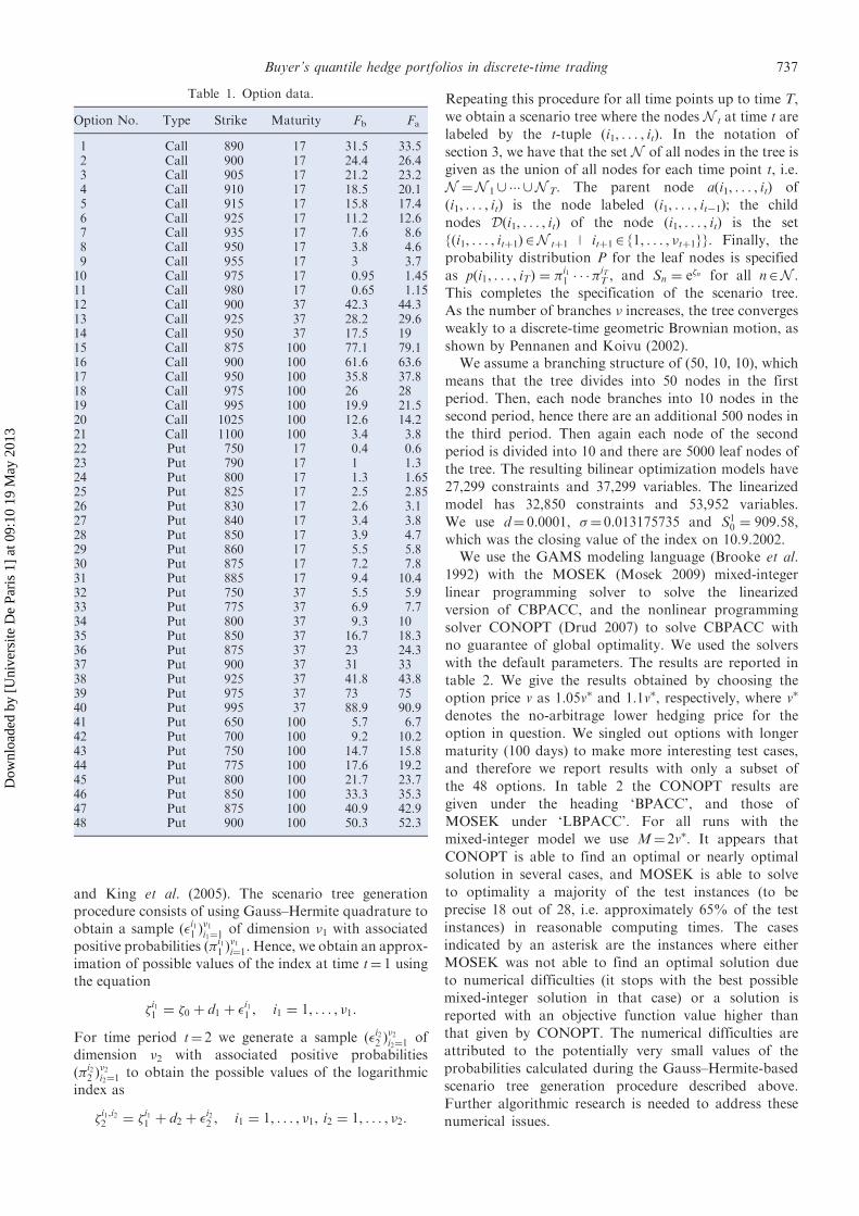
We use 48 European options written on the S&P 500index (table 1) in our computational experimentation.The option data were available in the market onSeptember 10, 2002. The first 21 of the options are calloptions and the remainder are put options. Strikes andmaturities as well as actual bid and ask prices (columns Fb

and Fa) of these options are given in table 1. To create atest case close to reality we treat a given option C as anAmerican option, while the remaining 47 options aretaken as European options to be used in buy-and-holdpolicies in hedging C. We repeat this exercise for 14 of theoptions given in table 1, namely call options numbered15–20 and those put options numbered 41–48.

We use a four period setting where we assume thatinvestors can trade at days 0, 17, 37 and 100. We useS¼ (1, S1) as the traded securities. Having S0

¼ 1 for alldates means that the interest rate is zero. We assume thatthe price of the S&P 500 index (i.e. S1) follows a geometricBrownian motion. Under this assumption, we generate ascenario tree by the Gauss–Hermite process discussed byOmberg (1988) and King et al. (2005) in detail. Theprocedure works as follows. We assume that the value S1

of the S&P 500 index evolves as a geometric Brownianmotion with daily drift d and volatility �. Let l be thelength of period t in days. Then, the logarithm �t ¼ lnS1

t

evolves according to

�t ¼ �t�1 þ dt þ �t,

where dt¼ ltd, and �t is normally distributed with zeromean and standard deviation �t ¼

ffiffiffiltp

�. Using givenparameters �0 and the initial values of �, lt, t¼ 1, . . . ,T, dand �, we construct a scenario tree approximation to thestochastic process �t using Gauss–Hermite quadrature asadvocated by Omberg (1988), Pennanen and Koivu (2002)

8 M.C. Pinar736

Dow

nloa

ded

by [

Uni

vers

ite D

e Pa

ris

1] a

t 09:

10 1

9 M

ay 2

013

and King et al. (2005). The scenario tree generationprocedure consists of using Gauss–Hermite quadrature toobtain a sample ð�i11 Þ

�1i1¼1

of dimension �1 with associatedpositive probabilities ð�i11 Þ

�1i¼1. Hence, we obtain an approx-

imation of possible values of the index at time t¼ 1 usingthe equation

�i11 ¼ �0 þ d1 þ �i11 , i1 ¼ 1, . . . , �1:

For time period t¼ 2 we generate a sample ð�i22 Þ�2i2¼1

ofdimension �2 with associated positive probabilitiesð�i22 Þ

�2i2¼1

to obtain the possible values of the logarithmicindex as

�i1,i22 ¼ �i11 þ d2 þ �i22 , i1 ¼ 1, . . . , �1, i2 ¼ 1, . . . , �2:

Repeating this procedure for all time points up to time T,

we obtain a scenario tree where the nodes N t at time t are

labeled by the t-tuple (i1, . . . , it). In the notation of

section 3, we have that the set N of all nodes in the tree is

given as the union of all nodes for each time point t, i.e.

N ¼N 1[ ��� [N T. The parent node a(i1, . . . , it) of

(i1, . . . , it) is the node labeled (i1, . . . , it�1); the child

nodes D(i1, . . . , it) of the node (i1, . . . , it) is the set

{(i1, . . . , itþ1)2N tþ1 | itþ12 {1, . . . , �tþ1}}. Finally, the

probability distribution P for the leaf nodes is specified

as pði1, . . . , iTÞ ¼ �i11 � � ��

iTT , and Sn ¼ e�n for all n2N .

This completes the specification of the scenario tree.

As the number of branches � increases, the tree convergesweakly to a discrete-time geometric Brownian motion, as

shown by Pennanen and Koivu (2002).We assume a branching structure of (50, 10, 10), which

means that the tree divides into 50 nodes in the first

period. Then, each node branches into 10 nodes in the

second period, hence there are an additional 500 nodes in

the third period. Then again each node of the second

period is divided into 10 and there are 5000 leaf nodes of

the tree. The resulting bilinear optimization models have

27,299 constraints and 37,299 variables. The linearized

model has 32,850 constraints and 53,952 variables.

We use d¼ 0.0001, �¼ 0.013175735 and S10 ¼ 909:58,

which was the closing value of the index on 10.9.2002.We use the GAMS modeling language (Brooke et al.

1992) with the MOSEK (Mosek 2009) mixed-integer

linear programming solver to solve the linearized

version of CBPACC, and the nonlinear programming

solver CONOPT (Drud 2007) to solve CBPACC with

no guarantee of global optimality. We used the solvers

with the default parameters. The results are reported in

table 2. We give the results obtained by choosing the

option price v as 1.05v� and 1.1v�, respectively, where v�

denotes the no-arbitrage lower hedging price for the

option in question. We singled out options with longer

maturity (100 days) to make more interesting test cases,

and therefore we report results with only a subset of

the 48 options. In table 2 the CONOPT results are

given under the heading ‘BPACC’, and those of

MOSEK under ‘LBPACC’. For all runs with the

mixed-integer model we use M¼ 2v�. It appears that

CONOPT is able to find an optimal or nearly optimal

solution in several cases, and MOSEK is able to solve

to optimality a majority of the test instances (to be

precise 18 out of 28, i.e. approximately 65% of the test

instances) in reasonable computing times. The cases

indicated by an asterisk are the instances where either

MOSEK was not able to find an optimal solution due

to numerical difficulties (it stops with the best possible

mixed-integer solution in that case) or a solution is

reported with an objective function value higher than

that given by CONOPT. The numerical difficulties are

attributed to the potentially very small values of the

probabilities calculated during the Gauss–Hermite-based

scenario tree generation procedure described above.

Further algorithmic research is needed to address these

numerical issues.

Table 1. Option data.

Option No. Type Strike Maturity Fb Fa

1 Call 890 17 31.5 33.52 Call 900 17 24.4 26.43 Call 905 17 21.2 23.24 Call 910 17 18.5 20.15 Call 915 17 15.8 17.46 Call 925 17 11.2 12.67 Call 935 17 7.6 8.68 Call 950 17 3.8 4.69 Call 955 17 3 3.710 Call 975 17 0.95 1.4511 Call 980 17 0.65 1.1512 Call 900 37 42.3 44.313 Call 925 37 28.2 29.614 Call 950 37 17.5 1915 Call 875 100 77.1 79.116 Call 900 100 61.6 63.617 Call 950 100 35.8 37.818 Call 975 100 26 2819 Call 995 100 19.9 21.520 Call 1025 100 12.6 14.221 Call 1100 100 3.4 3.822 Put 750 17 0.4 0.623 Put 790 17 1 1.324 Put 800 17 1.3 1.6525 Put 825 17 2.5 2.8526 Put 830 17 2.6 3.127 Put 840 17 3.4 3.828 Put 850 17 3.9 4.729 Put 860 17 5.5 5.830 Put 875 17 7.2 7.831 Put 885 17 9.4 10.432 Put 750 37 5.5 5.933 Put 775 37 6.9 7.734 Put 800 37 9.3 1035 Put 850 37 16.7 18.336 Put 875 37 23 24.337 Put 900 37 31 3338 Put 925 37 41.8 43.839 Put 975 37 73 7540 Put 995 37 88.9 90.941 Put 650 100 5.7 6.742 Put 700 100 9.2 10.243 Put 750 100 14.7 15.844 Put 775 100 17.6 19.245 Put 800 100 21.7 23.746 Put 850 100 33.3 35.347 Put 875 100 40.9 42.948 Put 900 100 50.3 52.3

Buyer’s quantile hedge portfolios in discrete-time trading 9737

Dow

nloa

ded

by [

Uni

vers

ite D

e Pa

ris

1] a

t 09:

10 1

9 M

ay 2

013

6. Conclusions

We have addressed the problem of quantile hedging forAmerican contingent claims from the perspective of thebuyer of a contingent claim in discrete-time financialmarkets. After a general exposition in a discrete-timeinfinite-state space setting we specialize our results to thefinite-dimensional probability setting. The specializationresulted in finite-dimensional optimization problemswhich turn out to be bilinear or mixed-integer linearprogramming problems. We have shown that the prob-lems can be processed numerically by state-of-the artsolvers with default parameters for the case of findingbuyer quantile hedge price bounds for S&P 500 optionsusing other such options as part of the hedge portfolio.

Acknowledgements

The assistance of Tardu S. Sepin with the numericalexperiments is gratefully acknowledged. The researchreported in this paper was partially supported byTUBITAK grant 107K250.

References

Bard, J.F., Practical Bilevel Optimization: Algorithms andApplications, 1998 (Kluwer Academic: Dordrecht).

Ben-Tal, A. and Nemirovski, A., Lectures on Modern ConvexOptimization: Analysis, Algorithms and EngineeringApplications, 2001 (MPS-SIAM Series on Optimization)(SIAM: Philadelphia).

Brooke, A., Kendrick, D. and Meeraus, A., GAMS: A User’sGuide, 1992 (The Scientific Press: San Fransisco).

Camci, A. and Pinar, M.C., Pricing American contingent claimsby stochastic linear programming. Optimization, 2009, 58(6),627–640.

Chalasani, P. and Jha, S., Randomized stopping times andAmerican option pricing with transaction costs.Math. Finance, 2001, 11, 33–77.

Drud, A., CONOPT Solver Manual, 2007 (ARKI Consulting:Bagsvaerd, Denmark).

Follmer, H. and Leukert, P., Quantile hedging. FinanceStochast., 2000, 3, 251–273.

Follmer, H. and Schied, A., Stochastic Finance: An Introductionin Discrete Time, 2nd ed., 2004 (De Gruyter Studies inMathematics) (De Gruyter: Berlin).

King, A.J., Duality and martingales: A stochastic programmingperspective on contingent claims. Math. Prog. Ser. B, 2002,91, 543–562.

King, A.J., Koivu, M. and Pennanen, T., Calibrated optionbounds. Int. J. Theor. Appl. Finance, 2005, 8(2), 141–159.

MOSEK Solver Manual, 2009 (Mosek ApS: Copenhagen).Nakano, Y., Minimizing coherent risk measures of shortfall indiscrete time models under cone constraints. Appl. Math.Finance, 2003, 10, 163–181.

Nakano, Y., Efficient hedging with coherent risk measures.J. Math. Anal. Applic., 2004, 293, 345–354.

Omberg, E., Efficient discrete time jump process models inoption pricing. J. Financial Quant. Anal., 1988, 23(2),161–174.

Pennanen, T. and King, A., Arbitrage pricing of Americancontingent claims in incomplete markets – A convexoptimization approach. Working Paper, 2006. Availableonline at: math.tkk.fi/teemu/american.pdf

Pennanen, T. and Koivu, M., Integration quadratures indiscretization of stochastic programs. StochasticProgramming E-Print Series, 2002.

Perez-Hernandez, L., On the existence of an efficient hedge foran American contingent claim within a discrete time market.Quant. Finance, 2007, 7, 547–551.

Rudloff, B., Convex hedging in incomplete markets.Appl. Math. Finance, 2007, 14, 437–452.

Rudloff, B., Coherent hedging in incomplete markets.Quant. Finance, 2009, 9, 197–206.

Schrijver, A., Theory of Linear and Integer Programming, 1986(Wiley: Chichester).

Spivak, G. and Cvitanic, J., Maximizing the probability of aperfect hedge. Ann. Appl. Probab., 1999, 9, 1303–1328.

Van Tiel, J., Convex Analysis: An Introductory Text, 1984(Wiley: Chichester).

Table 2. Numerical results with S&P 500 options using MOSEK and CONOPT solvers.

Results for %5 Expanded prices Results for %10 Expanded prices

Option properties BPACC LBPACC BPACC LBPACC

Type Strike Objective value Time Objective value Time Objective value Time Objective value Time

Call 875 1.0177 268.50 19.26� 478.43 1.1543 155.12 2.40� 423.77Call 900 1.0153 276.04 12.49� 507.38 1.0306 298.62 13.17� 562.34Call 950 1.0042 458.61 1.0042 308.28 1.0123 396.01 1.0123 631.49Call 975 1.0035 405.30 1.0034 146.50 1.0101 349.37 1.0101 1314.68Call 995 1.0027 417.43 1.0027 41.00 1.0079 287.57 1.0079 1248.10Call 1025 1.0002 316.85 1.0002 136.39 1.0010 301.88 1.0010 69.68Put 650 1.0001 124.80 1.0001 155.97 1.0001 145.55 1.0002� 35.22Put 700 1.00002 21.25 1.00003� 112.74 1.00002 22.01 1.0002� 31.88Put 750 1.00002 82.06 1.00002 116.65 1.00002 82.47 1.00002� 967.43Put 775 1.00003 103.19 1.00003 125.29 1.00005 133.31 1.00006� 22.91Put 800 Infeasible 1.0001 583.10 1.00005 152.51Put 850 1.0001 796.48 1.0001 151.05 1.0001 1266.20 1.0001 208.56Put 875 1.0001 1020.71 1.00005 774.50 1.0001 1254.80 1.0001 1093.06Put 900 1.0001 995.81 1.0001 775.39 1.0001 1751.11 1.0001 189.83

10 M.C. Pinar738

Dow

nloa

ded

by [

Uni

vers

ite D

e Pa

ris

1] a

t 09:

10 1

9 M

ay 2

013