arX

iv:h

ep-p

h/03

0213

0v1

16

Feb

2003

Bose-Einstein and Fermi-Dirac Interferometry

in Particle Physics

GIDEON ALEXANDER

School of Physics and AstronomyRaymond and Beverly Sackler Faculty of Exact Sciences

Tel-Aviv University, Tel-Aviv 69978, Israel

Abstract

The application of the Bose-Einstein and Fermi-Dirac interferometry to multi-hadronfinal states of particle reactions is reviewed. The underlying theoretical concepts of parti-cle interferometry is presented where a special emphasis is given to the recently proposedFermi-Dirac correlation analysis. The experimental tools used for the interferometry anal-yses and the interpretation of their results are discussed in some details. In particularthe interpretation of the dimension r, as measured from the interferometry analysis, isinvestigated and compared to that measured in heavy-ion collisions. Finally the similaritybetween the dependence of r on the hadron mass and the interatomic separation on theatomic mass in Bose condensates is outlined.

Contents

1 Introduction 2

2 Basic concepts in particle interferometry 42.1 The Bose-Einstein correlation of two hadrons . . . . . . . . . . . . . . . . . . . . 42.2 The Kopylov-Podgoretskii parametrisation . . . . . . . . . . . . . . . . . . . . . 62.3 Higher order Bose-Einstein correlations . . . . . . . . . . . . . . . . . . . . . . . 72.4 Bose-Einstein correlation in two and three dimensions . . . . . . . . . . . . . . . 9

3 Fermi-Dirac correlation 103.1 The spin-spin correlation . . . . . . . . . . . . . . . . . . . . . . . . . . . . . . . 113.2 The phase space density approach . . . . . . . . . . . . . . . . . . . . . . . . . . 13

4 Experimental procedure and data analysis 144.1 Choice of the reference sample . . . . . . . . . . . . . . . . . . . . . . . . . . . . 15

4.1.1 Reference samples derived from the data . . . . . . . . . . . . . . . . . . 154.1.2 Monte Carlo generated reference samples . . . . . . . . . . . . . . . . . . 16

4.2 Final state interactions . . . . . . . . . . . . . . . . . . . . . . . . . . . . . . . . 184.2.1 The Coulomb effect . . . . . . . . . . . . . . . . . . . . . . . . . . . . . . 184.2.2 Strong final state interactions . . . . . . . . . . . . . . . . . . . . . . . . 19

5 The 1-Dimensional correlation results 195.1 The ππ Bose-Einstein correlation . . . . . . . . . . . . . . . . . . . . . . . . . . 195.2 The K±K± and K0

SK0S systems . . . . . . . . . . . . . . . . . . . . . . . . . . . 21

5.3 Isospin invariance and generalised Bose-Einstein correlation . . . . . . . . . . . . 245.4 Observation of higher order Bose-Einstein correlations . . . . . . . . . . . . . . . 255.5 Experimental results from Fermi-Dirac correlation analyses . . . . . . . . . . . . 26

6 The r dependence on the hadron mass 276.1 The r(m) description in terms of the Heisenberg relations . . . . . . . . . . . . . 286.2 QCD description of r(m) via the virial theorem . . . . . . . . . . . . . . . . . . 29

7 Results from multi-dimensional Bose-Einstein correlation analyses 317.1 rz(mT) description in terms of the Heisenberg relations . . . . . . . . . . . . . . 327.2 Application of the Bjorken-Gottfried relation to r(mT ) . . . . . . . . . . . . . . 347.3 r(m) and the interatomic separation in Bose condensates . . . . . . . . . . . . . 34

8 On the relation between r and the emitter size 378.1 The r dependence on the number of emitting sources . . . . . . . . . . . . . . . 39

9 Summary and conclusions 40

1

1 Introduction

The two-particle intensity interferometry (intensity correlation) method has been worked outand exploited for the first time in the 1950’s by Hanbury-Brown and Twiss (HBT) [1–3] to cor-relate intensity of electro-magnetic radiation, arriving from extraterrestrial radio-wave sources,and thus measure the angular diameter of stars and other astronomical objects. This methodrests on the fact that bosons obey the Bose-Einstein statistics so that the symmetrisation ofthe multi-particle wave function affects the measured many-particle coincident spectra to leadto an enhancement, relative to the single particle spectra, whenever they are emitted close byin time-phase space. Thus the interest in the Bose-Einstein correlation properties was not onlyrestricted to their fundamental quantum theoretical aspects but above all as a tool in the studyof the properties and spatial extent of sources emitting radiation and particles in the fields ofastronomy, and non-perturbative QCD aspects of particles and nuclei interactions.

Figure 1: The two indistinguishable diagrams that describe the emission of two identical bosons, π1and π2, emerging from the two points, r1 and r2, which lie within an emitter volume, and are detectedat the positions x1 and x2.

The difference between the intensity interferometry and the conventional amplitude interfer-ometry can be illustrated [4,5] with the help of Fig. 1. Consider a finite source which emits twoindistinguishable particles from the positions r1 and r2 which are later observed at positions x1and x2. In an amplitude interferometry the positions x1 and x2 could be a slit through whichthe emitted particles pass. The particles could then produce an interference pattern whichwill depend on the relative phase of the particle’s amplitude as measured at x1 and x2. In an

intensity interferometry a normalised correlation function∼

K (1, 2) of the particles 1 and 2 isformed from the average number 〈n1,2〉 of counts where n1 and n2 are detected simultaneouslyat x1 and x2:

∼

K (1, 2) =〈n1,2〉

〈n1〉〈n2〉− 1 . (1)

The correlation function is thus proportional to the intensity of the particles at x1 and x2.Because of the symmetrisation of their wave function, identical particles can have a nonzerocorrelation function even if the particles are otherwise noninteracting.

As can be expected intensity interferometry is closely related to the amplitude interferometrywhich essentially measures the square of the amplitudes A1 and A2 falling on the detectors x1and x2:

|A1 + A2|2 = |A1|2 + |A2|2 + (A⋆1A2 + A1A

⋆2) ,

where the last term is the fringe visibility denoted by V , which is the part of the signal whichis sensitive to the separation between the emission points. Averaged over random variations its

2

square is given by the product of the intensities landing on the two detectors:

〈V 2〉 = 2〈|A1|2|A2|2〉 + 〈A⋆21 A

22〉 + 〈A2

1A⋆22 〉 → 2〈I1I2〉 .

Since the last two terms of the 〈V 2〉 expression vary rapidly and average to zero, 〈V 2〉 is pro-portional to the time averaged correlation of the product of the two intensities (see e.g. Ref. [6]).

The Bose-Einstein correlation (BEC) analysis method was for the first time introduced in1959/60 by Goldhaber, Goldhaber, Lee and Pais (GGLP) [7, 8] to the hadron sector in orderto study the time-space structure of identical pions produced in particle interactions. Theirobservation of a BEC enhancement of pion-pairs emerging from pp annihilations at small rela-tive momenta was parametrised in terms of the finite spatial extension of the pp source and thefinite localisation of the decay pions. The momentum range of the enhancement could then berelated to the size of the particle source in space coordinates. Since then the boson interferome-try has been used extensively in variety of particle interactions and over a wide range of energies.

In the mid 1990’s the boson intensity interferometry measurement method has been ex-tended to the spin 1/2 baryon sector utilising the Fermi-Dirac statistical properties and inparticular the Pauli exclusion principle [9]. Already the results from the first attempt to studythe Fermi-Dirac correlation (FDC) of the ΛΛ and ΛΛ pairs, emerging from the decay of thegauge Z0 boson, indicated that the spatial extension of the hadron source is strongly dependenton its mass.

0

1

2

3

4

5

6

7

8

9

0 2 4A1/3

r rms(

fm)

Figure 2: An early compilation of values obtained for the emitter dimension rrms, extracted frominterferometry analyses of identical charged pion-pairs produced in heavy ion collisions are displayedas a function of A1/3 where A is the atomic number of the projectile. The values are taken fromRef. [10] and whenever more than one value is quoted for a given projectile nucleus, the plotted datapoints represent the average weighted values. The solid line represents the relation rrms = 1.2×A1/3

fm.

In parallel to the BEC studies of hadronic final states produced in particle reactions, ex-tensive pion-pair correlation analyses were and are applied to heavy ion collisions in order toexplore the characteristics of these rather complex reactions [6, 11, 12]. A compilation, taken

3

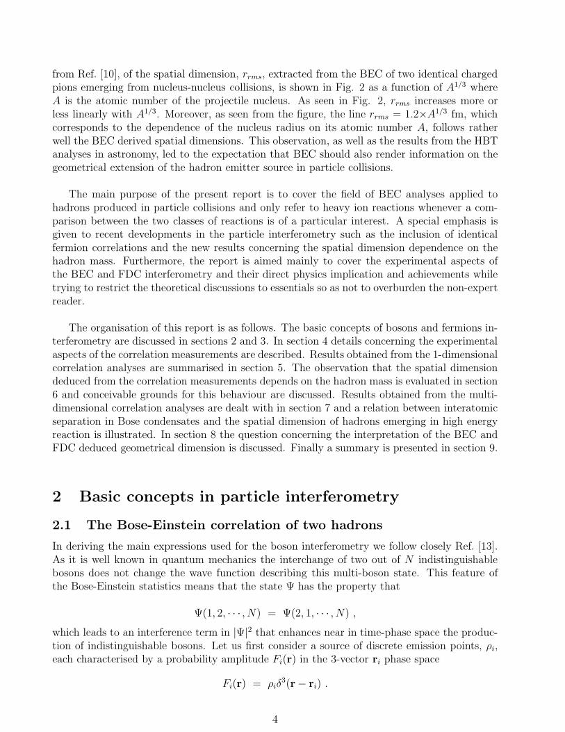
from Ref. [10], of the spatial dimension, rrms, extracted from the BEC of two identical chargedpions emerging from nucleus-nucleus collisions, is shown in Fig. 2 as a function of A1/3 whereA is the atomic number of the projectile nucleus. As seen in Fig. 2, rrms increases more orless linearly with A1/3. Moreover, as seen from the figure, the line rrms = 1.2×A1/3 fm, whichcorresponds to the dependence of the nucleus radius on its atomic number A, follows ratherwell the BEC derived spatial dimensions. This observation, as well as the results from the HBTanalyses in astronomy, led to the expectation that BEC should also render information on thegeometrical extension of the hadron emitter source in particle collisions.

The main purpose of the present report is to cover the field of BEC analyses applied tohadrons produced in particle collisions and only refer to heavy ion reactions whenever a com-parison between the two classes of reactions is of a particular interest. A special emphasis isgiven to recent developments in the particle interferometry such as the inclusion of identicalfermion correlations and the new results concerning the spatial dimension dependence on thehadron mass. Furthermore, the report is aimed mainly to cover the experimental aspects ofthe BEC and FDC interferometry and their direct physics implication and achievements whiletrying to restrict the theoretical discussions to essentials so as not to overburden the non-expertreader.

The organisation of this report is as follows. The basic concepts of bosons and fermions in-terferometry are discussed in sections 2 and 3. In section 4 details concerning the experimentalaspects of the correlation measurements are described. Results obtained from the 1-dimensionalcorrelation analyses are summarised in section 5. The observation that the spatial dimensiondeduced from the correlation measurements depends on the hadron mass is evaluated in section6 and conceivable grounds for this behaviour are discussed. Results obtained from the multi-dimensional correlation analyses are dealt with in section 7 and a relation between interatomicseparation in Bose condensates and the spatial dimension of hadrons emerging in high energyreaction is illustrated. In section 8 the question concerning the interpretation of the BEC andFDC deduced geometrical dimension is discussed. Finally a summary is presented in section 9.

2 Basic concepts in particle interferometry

2.1 The Bose-Einstein correlation of two hadrons

In deriving the main expressions used for the boson interferometry we follow closely Ref. [13].As it is well known in quantum mechanics the interchange of two out of N indistinguishablebosons does not change the wave function describing this multi-boson state. This feature ofthe Bose-Einstein statistics means that the state Ψ has the property that

Ψ(1, 2, · · · , N) = Ψ(2, 1, · · · , N) ,

which leads to an interference term in |Ψ|2 that enhances near in time-phase space the produc-tion of indistinguishable bosons. Let us first consider a source of discrete emission points, ρi,each characterised by a probability amplitude Fi(r) in the 3-vector ri phase space

Fi(r) = ρiδ3(r− ri) .

4

Next we introduce the central assumption pertaining to the BEC effect namely, the chaoticor the total incoherence limit, which corresponds to the situation where the phases of theproduction amplitudes wildly fluctuate in every point of space. In this limit all the phases canbe set to zero. If ψk(r) is the wave function of the emitted particle, then the total probabilityP (k) to observe the emission of one particle with a 3-momentum vector k is given by summingup the contributions from all the i points, that is

P (k) =∑

i

|ρiψ(ri)|2 .

For simplicity we will further use plane wave functions ψk ∝ ei(kr+φ) where in the incoherentcase we can set φ = 0. Next we replace the sum by an integral so that

P (k) =∫

|ρ(r)|2d3r . (2)

The probability to observe two particles with momenta k1 and k2 is

P (k1,k2) =∫

|ψ1,2|2|ρ(r1)|2|ρ(r2)|2d3r1d3r2 , (3)

where ψ1,2 = ψ1,2(k1,k2, r1, r2) is the two-particle wave function.

Taking incoherent plane waves, then for two identical bosons the symmetrised ψ1,2 is of theform

ψs1,2 =

1√2

[

ei(k1r1+k2r2) + ei(k1r2+k2r1)]

(4)

so that|ψs

1,2|2 = 1 + cos[(k1 − k2)(r1 − r2)] = 1 + cos[∆k(r1 − r2)] . (5)

Using Eqs. (2), (3) and (5) one can define a second order correlation function

C2(k1,k2) ≡P (k1,k2)

P (k1)P (k2)= 1 +

∫

cos[∆k(r1 − r2)]|ρ(r1)|2|ρ(r2)|2d3r1d3r2P (k1)P (k2)

, (6)

where ∆k = k1 −k2. Assuming that the emitter extension ρ(r) is localised in space and timethen it follows that when ∆k = 0 the last term of Eq. (6) can vary between the values 0 to1. From Eq. (6) one obtains after integration (Fourier transformation)

C2(∆k) = 1 + |ρ(∆k)|2 .

In many of the two-boson one dimensional BEC analyses one uses the Lorentz invariant param-eter Q, defined as Q2 = Q2

2 = −(q1−q2)2 ≡ M22 − 4µ2. Here q1, q2 andM

22 are respectively

the 4-momentum vectors and the invariant mass squared of the two identical bosons of mass µ.Thus one obtains

C2(Q) = 1 + |ρ(Q)|2 . (7)

Assuming further that the source is described by a spherical symmetric Gaussian density dis-tribution of emitting centres

ρ(r) = ρ(0)e− r2

2r20 ,

then the Bose-Einstein correlation function assumes the form

C2(∆k) = 1 + e−r20∆k2

.

5

In terms of the variable Q and the dimension rG, introduced by Goldhaber et al. [7, 8], thecorrelation function in the completely chaotic limit is equal to

C2(Q) = 1 + e−r2GQ2

. (8)

In the completely coherent case it can be shown [14] that C2(Q) = 1. In order to accommodatethose cases where the source is not completely chaotic one introduces a chaoticity parameterλ2 which can vary between the value 0, corresponding to a complete coherent case, to the value1 at the total chaotic limit. Thus Eq. (8) is transformed to the GGLP form

C2(Q) = N(1 + λ2e−r2

GQ2

) , (9)

where N is added as a normalisation factor. Since the strength of the BEC effect dependsalso on the experimental data quality, like the purity of the identical boson sample, λ2 is oftenalso referred to as the BEC strength parameter. In the following, unless otherwise stated,we will denote by r the dimension values obtained from BEC analyses which used the GGLPparametrisation, that is r ≡ rG. Two examples of a typical behaviour of the correlation functionC2(Q) of identical charged pion-pairs are shown in Fig. 3. The first are the results of OPAL [15]where the pion-pairs were taken from the hadronic Z0 decays and the second reported by theZEUS collaboration [16] in their study of the deep inelastic ep scattering produced at the HERAcollider.

0.8

1

1.2

1.4

1.6

1.8

0 0.5 1 1.5 2

with FSI

without FSI

N(±

±)/N

BG

Q [GeV/c]

OPAL

Q (GeV)

C

ZEUS

+

Q

2

> 110 GeV

2

ZEUS (prel.) 98-00

Æ (in luded in the �t)

�

0

K

0

S

Figure 3: The π±π± BEC as a function of Q. Left: OPAL results [15] obtained in the hadronic Z0

decays. The solid and dashed lines represent the fit results of Ref. [17] respectively with and withoutthe inclusion of final state interactions (see Sec. 4.2). Right: ZEUS results obtained in deep inelasticep scattering with momentum transfer of Q2 > 110 GeV2 [16]. The regions of K0

S and ρ0 which wereomitted from the fit of the correlation function C2(Q) are indicated.

2.2 The Kopylov-Podgoretskii parametrisation

In addition to the Goldhaber parametrisation, given by Eq. (9), another favourite parametri-sation is that proposed by Kopylov and Podgoretskii (KP) [18–20] which corresponds to a

6

radiating sphere surface of radius rKP with incoherent point-like oscillators of lifetime τ , namely

C(qt, q0) = 1 + λ[4J21 (qtrKP )/(qtr

2KP ]/[1 + (q0τ)

2] , (10)

where J1 is the first-order Bessel function. Here q0 is equal to |E1 − E2| and qt = |q × k|/|k|where k = k1+k2, the sum of the two hadron momenta and q = k1−k2 is the difference betweenthem. This correlation expression is not Lorentz invariant and its variables are calculated inthe centre of mass system (CMS) of the final state hadrons. The correlation function C(qt, q0)can be written in terms of the Goldhaber geometrical parameter rG as [21]

C(qt, q0) = 1 + λ exp[−r2Gq2t − r2Gq20/(γ

2 − 1)] , (11)

where γ is the γ−factor of the identical boson pair. From a comparison between Eqs. (11) and(9) it is clear that the parameters rG and rKP have different interpretations. At small qt andq0, however, the parametrisation (10) can be approximated to be

C(qt, q0) = 1 + λ exp[−(rKP/2)2q2t − (q0τ)

2] . (12)

From Eqs. (11) and (12) one finds the approximate relation rKP ≃ 2rG which is verified ex-perimentally. For example, in a study [22] of the BEC of the π±π± system emerging from thedecay of the Z0 boson one obtained rG = 0.955 ± 0.012(stat.) ± 0.015(syst.) fm as comparedto rKP = 1.778± 0.023(stat.)± 0.036(syst.) fm.

In contrast to the rather simple and straightforward BEC analysis offered by the GGLPparametrisation, the KP method expects a correlation enhancement at low, near zero, q0 valuesso that the analysis is carried out in several q0 energy slices. In addition the KP formalismhas an extra free parameter, (q0τ)

2, which has to be determined through a fit to the data.For these reasons the KP correlation investigations require higher statistical data samples thanthose needed for the BEC analysis in the GGLP method.

2.3 Higher order Bose-Einstein correlations

A Bose-Einstein correlation enhancement is also expected to be present in identical bosonsystems of more than two particles when they emerge from the interaction within a small time-space region. In the search for these so called, higher order BEC enhancements, one has todifferentiate between those produced from the lower BEC order(s) and those who are genuinecorrelations. The normalised over-all inclusive correlations of n identical bosons is given by [23]

Rn =ρn(p1, p2 · · · pn)

ρ1(p1)ρ1(p2) · · · ρ1(pn)= σn−1 dnσ

dp1dp2 · · · dpn

/

dσ

dp1

dσ

dp2· · · dσ

dpn

, (13)

where σ is the total boson production cross section, ρ1(pi) and dσ/dpi are the single-boson den-sity in momentum space and the inclusive cross section, respectively. Similarly ρn(p1, p2 · · · pn)and dnσ/(dp1dp2 · · · dpn) are respectively the density of the n-boson system and its inclusivecross section. The product of the independent one-particle densities ρ1(p1)ρ1(p2) · · · ρ1(pn) isreferred to as the reference density distribution, or reference sample, to which the measuredcorrelations are compared to. Specifically the inclusive two-boson density ρ2(p1, p2) can bewritten as:

ρ2(p1, p2) = ρ1(p1)ρ1(p2) +K2(p1, p2) , (14)

7

where ρ1(p1)ρ1(p2) represents the two independent boson momentum spectra and K2(p1, p2)describes the two-body correlations. In this simple case of two identical bosons the normaliseddensity function R2, defined by Eq. (13), already measures the genuine two-body correlationswhich here (see Sec. 2.1) is referred to as the C2 correlation function. Thus one has

C2 ≡ R2 = 1+∼

K2 (p1, p2) , (15)

where∼

K2 (p1, p2) = K2(p1, p2)/[ρ1(p1)ρ1(p2)] is the normalised two-body correlation term whichin the GGLP parametrisation defined in Eq. (9), is equal to λ2 exp(−Q2

2r22).

The inclusive correlation of three identical bosons, ρ3(p1, p2, p3), includes the three indepen-dent boson momentum spectra, the two-particle correlation K2 and the genuine three-particlecorrelation K3, namely:

ρ3(p1, p2, p3) = ρ1(p1)ρ1(p2)ρ1(p3) +∑

(3)

ρ1(pi)K2(pj, pk) +K3(p1, p2, p3) , (16)

where the summation is taken over all the three possible permutations. The normalised inclusivethree-body density, is then given by

R3 =ρ3(p1, p2, p3)

ρ1(p1)ρ1(p2)ρ1(p3)= 1 +R1,2+

∼

K3 (p1, p2, p3) . (17)

Here

R1,2 =

∑

(3) ρ1(pi)K2(pj , pk)

ρ1(p1)ρ1(p2)ρ1(p3)and

∼

K3 (p1, p2, p3) =K3(p1, p2, p3)

ρ1(p1)ρ1(p2)ρ1(p3)

represent the mixed three-boson system in which only two of them are correlated and the three-boson correlation. In analogy to C2, one defines a correlation function C3 which measures thegenuine three-boson correlation, by subtracting from R3 the term which contains the two-bosoncorrelation contribution. Thus

C3 ≡ R3 −R1,2 = 1+∼

K3 (p1, p2, p3) , (18)

which depends only on the genuine three-boson correlation. For the study of the three-bosoncorrelation one often uses the variable Q3 which, analogous to the variable Q2

2, is defined as

Q23 =

∑

(3)

q2i,j = M23 − 9µ2 ,

where the summation is taken over all the three different i, j boson-pairs. Here M23 is the

invariant mass squared of the three-boson system and µ is the mass of the single boson. Fromthe definition of this three-boson variable it is clear that asQ3 approaches zero so do all the threerelated qi,j values which eventually reach the region where the two-boson BEC enhancementsare observed. It has been shown [24] that the genuine three-pion correlation function C3(Q3)can be parametrised by the expression

C3(Q3) = 1 + 2λ3e−Q2

3r23 , (19)

where λ3 is the chaoticity parameter which may assume a value between zero and one.

8

The method outlined here for the extraction of the three-boson BEC enhancement can inprinciple be extended to higher orders, however it becomes too cumbersome to be of a practicaluse and on top of it, it requires very high statistics data. For these reasons two other approacheshave been advocated and utilised experimentally. In the first, one measures experimentally theover-all correlation, as defined by Rn in Eq. (13), and then with the help of various modelsone tries to extract the higher order genuine BEC parameters rn and λn. Such an approach isadopted for example in references [25,26]. In the second approach one analyses the data in termsof correlation functions [27, 28] known as factorial cumulant moments or, in their integratedform are referred to as the semi-invariant cumulants of Thiele which constitutes an importantelement in proving the central limit theorem in statistics (see e.g. [29]). Having n particlesin a given domain then the corresponding factorial cumulant moments will be different fromzero only if a genuine n-particle correlation exists. The shortcoming of the cumulant approachis however the fact that its results for a given higher order (n ≥ 3) pertain to the overallgenuine correlation present in the data so that the partial contribution of the genuine BEC,parametrised by rn and λn is not transparent.

2.4 Bose-Einstein correlation in two and three dimensions

In the GGLP interferometry analysis the emitter shape is considered to be of a spherical shapewith a Gaussian density distribution. A method to explore the possibility that the time-spaceextent of the particle emission region deviates from a sphere, and in fact is characterised bymore than one dimension, has been recently proposed [11,30,31]. To this end the BEC analysisis carried out in the Longitudinal Centre-of-Mass System (LCMS) shown schematically in Fig.4. This coordinate system is defined for each pair of identical bosons as the system in which

Qlong

Q t,side

t,out

Q

p+p

p

Quark / jet / thrust

1

p1

2

21

p-p2

Figure 4: The Longitudinal Centre-of-Mass-System coordinates (taken from Ref. [32]).

the sum of the boson-pair 3-momenta p1 + p2, referred to as the out - axis, is perpendicular tothe thrust (or jet) direction of the multi-hadron event defined as the z - axis (≡ long - axis).The momentum difference of the pion-pair Q is then resolved into the longitudinal directionQz ≡ Q|| parallel to the thrust axis, to the Qout - axis which is collinear with the pair momentasum and the third axis, Qside which is perpendicular to both Qz and Qout. In this system theprojections of the total momentum of the particle-pair onto the longitudinal and side directions

9

are equal to zero. The total Q2 value is given by

Q2 = Q2z +Q2

side +Q2out(1− β2), where β =

p1,out + p2,outE1 + E2

. (20)

Here the indices 1 and 2 refer to the first and second boson. Since p1,z = −p2,z one has

Qz = Q‖ = p1,z − p2,z = 2p1,z = 2pz .

The difference in the emission time of the pions, which couples to the energy difference betweenthem, appears only in the Qout direction. The 3-dimension correlation function is given by

C2(Qz, Qside, Qout) = 1 + λ2e−(r2zQ

2z + r2

sideQ2

side+ r2outQ

2

out) . (21)

In many cases due to lack of sufficient statistics, one wishes to reduce the number of pa-rameters to be fitted in the correlation function by defining the transverse component rT in theLCMS to be r2T = r2side + r2out corresponding to

Q2T = Q2

out + Q2side .

Thus the correlation function, which is fitted to the data, is of the form

C2(Qz, QT ) = 1 + λ2e−(r2zQ

2z + r2

TQ2

T) , (22)

where rz, estimated from Eq. (22) as Qz approaches zero, is the longitudinal geometrical radiusand rT is composed of the transverse radius and the emission time difference. The experimentalfindings in heavy ion collisions [33, 34], in hadron-hadron reactions [35, 36] and e+e− annihila-tions [37–39], verify the theoretical expectations of the Lund string model [40,41] that the ratiorT/rz is significantly smaller than one (see Sec. 4.1.2).

The assignment of a well defined physical direction in the LCMS, such as thrust axis, allowsto study in the framework of the BEC analysis an additional meaningful variable namely, theaverage transverse mass mT of the two identical hadrons. This transverse mass is defined as

mT =1

2[m1,T + m2,T ] =

1

2

[√

m21 + p21,T +

√

m22 + p22,T

]

, (23)

where the indices 1 and 2 refer to the first and second hadron.

3 Fermi-Dirac correlation

The application of two-boson correlation to the estimation of an r dimension has recently beenextended to identical pairs of fermions (baryons) [9]. This extension is based on the Fermi-Diracstatistics feature which prohibit the total spin to have the value S = S1+S2 = 1 when the twoidentical fermions are in an s-wave (ℓ = 0) state. Thus in the so called Fermi-Dirac correlation(FDC) method one can, similarly to the BEC analysis, study the contributions of the S = 0 andS = 1 states to the di-fermion system as Q approaches zero where, in the absence of di-baryonresonances, only the s-wave state survives.

The estimation of r from the rate of depletion of the S = 1 population as Q → 0 can beachieved in two ways. The first consists of a direct measurement of the relative contributions ofS = 1 and S = 0 spin states to the di-baryon system as a function of Q (see next section). Analternative method consists of a measurement of the di-baryon density decrease as Q approacheszero, assuming its origin to be due to the Pauli exclusion principle. This second method isequivalent to that used in the BEC analysis of two identical bosons.

10

3.1 The spin-spin correlation

If F0(Q) and F1(Q) are respectively the fraction of the S = 0 and the S = 1 contributions, ata given Q value, to the di-baryon system then one can e.g. study two correlation functions,CS=0(Q) and CS=1(Q), defined by the ratios:

C0(Q) =2F0(Q)

F0(Q) + F1(Q)/3and C1(Q) =

2F1(Q)/3

F0(Q) + F1(Q)/3,

where F1(Q) is divided by 3 to offset the statistical 2S+1 spin factor. At high Q values, where

Q (Arbitrary Units)

C (

Q)

(a)

S = 0

S =

1

0

0.2

0.4

0.6

0.8

1

1.2

1.4

1.6

1.8

2

0 0.1 0.2 0.3 0.4 0.5 0.6 0.7 0.8 0.9 10

0.2

0.4

0.6

0.8

1

1.2

1.4

1.6

1.8

2

-1 -0.8 -0.6 -0.4 -0.2 0 0.2 0.4 0.6 0.8 1y

1/N

dN

/dy

(b)

S = 1

S = 0

Figure 5: (a) Schematic view of the FDC functions C0 and C1 dependence on Q, for the S = 0 andS = 1 states, of an identical spin 1/2 two-baryon system. The dashed line represents the expectationfor a baryon anti-baryon system in the absence of resonances. (b) The (1/N)dN/dy behaviour of theS = 0 and S = 1 states of a two identical baryons sample.

the highest angular momentum ℓmax is large, one may expect that C0∼= C1

∼= 1 correspondingto a statistical spin mixture ensemble. On the other hand when Q = 0, one will observeC0 ≈ 2 and C1 ≈ 0. Thus the C0 behaviour as a function of Q is similar to the BEC functionC2(Q), of two identical mesons, which rises as the ℓmax → 0. As for the di-baryon correlationfunction C1(Q) there is no parallel case in the identical charged di-boson system. One furtherassumes the emitter to be a sphere with a Gaussian distribution so that, analogous to the BECparametrisation, the di-baryon correlation functions can be parametrised as [9]:

C0(Q) = 1 + λe−r2Q2

and C1(Q) = 1− λe−r2Q2

.

Here the λ parameter, which can vary between 0 and 1, measures the strength of the effect andis mainly sensitive to the purity of the data sample. A schematic view of the dependence ofC0 and C1 on Q is shown in Fig. 5a. The study of either C0 or C1 can render a value for rhowever, since the diminishing contribution of the S = 1 state is responsible for the variationof the correlation function as Q decreases, one usually analyses C1. Here it should be notedthat unlike the BEC effect which can be extended to many-boson states, the FDC is limited totwo identical fermions since already the third one is in an ℓ > 0 state (Pauli exclusion principle).

11

A general method for the direct measurement of the total spin composition of any two spin1/2 baryons system which decay weakly has been outlined in reference [9]. Here we illustratethis method (later referred as Method I) in its application to the ΛΛ and the ΛΛ systems. Thesimplest measurable case is the one where the Λ decays into p1 + π− and the other Λ, or Λ, top2 + π+ where pi stands for the decay proton or anti-proton both of which we will further referto as protons. Let us further denote by y the cosine of the angle (in space) between p1 andp2 and 〈y〉 as its average, defined in a system reached after two transformations. The first, tothe CMS of the di-Λ pair and the second where each proton is transformed to the CMS of itsparent Λ. To note is that at Q = 0 the second transformation is superfluous.

In the decay of a single Λ, the proton angular distribution with respect to the spin directionin the centre of mass, is given by [42]:

dw/d cos θ ∝ 1− αΛ cos θ , (24)

where the parity violating parameter αΛ = −αΛ was measured experimentally [43] to be0.642 ± 0.013. Setting x = cos θ the average 〈xΛ〉 is given by:

〈xΛ〉 =1

2πN

∫ 2π

0dφ∫ xmax

xmin

(1− αΛx)xdx where N =∫ xmax

xmin

(1− αΛx)dx . (25)

In particular, the average over the whole angular range from xmin = −1 to xmax = +1 yields

〈xΛ〉 = −0.214± 0.004 and 〈xΛ〉 = +0.214± 0.004 .

General arguments do not allow dN/dy distribution of a two spin-1/2 hyperon system atthreshold to have a y dependence higher than its first power. This means that dN/dy is of theform

dN/dy = A[1 +BS y] .

The factor BS can then be determined independent of the total angular momentum J value atQ = 0 or nearby from the value of 〈y〉 using the Wigner-Eckart theorem [44, 45]. Thus for theΛΛ and ΛΛ pairs one obtains

BS=0 = −9 〈xΛ〉2 = −0.4122 and BS=1 = +3 〈xΛ〉2 = +0.1374 .

As a result one then has for the ΛΛ(ΛΛ) system at, or very near, its threshold

dN/dy|S=0

∝ 1− 0.4122y and dN/dy|S=1

∝ 1 + 0.1374y . (26)

To note is that the ℓ = 0, S = 1 state is forbidden by the Pauli principle. These two distinctlydifferent distributions, are shown in Fig. 5b. In a similar way one obtains for the ΛΛ system

dN/dy|S=0

∝ 1 + 0.4122y and dN/dy|S=1

∝ 1− 0.1374y . (27)

Even though the Wigner-Eckart theorem is applicable to the di-baryon system at Q = 0, it isshown in Ref. [9] that Eqs. (26) and (27) can also be applied to at Q > 0 as long as the protonsemerging from the Λ decays are non-relativistic. That this method can be extended even tohigher Q values has been pointed out in Ref. [46]. If the parameter ǫ is defined as the fractionof the S = 1 contribution to the two-baryon system then it can be measured as a function of

12

Q by fitting the expression

dN/dy = (1 − ǫ) dN/dy|S=0 + ǫ dN/dy|S=1 , (28)

to the data. In the case of a statistical spin mixture, ǫ is equal to 0.75 which yields a constantdN/dy distribution. This spin analysis method has the advantage that it directly measuresthe S =1 depletion as expected from the Pauli principle. In addition it does not require anyreference sample which, as is well known from the BEC analyses, is the major contributor tothe systematic errors of the measurement (see Sec. 4.1). The main disadvantage of the directspin measurement is its need for a rather large data sample. In addition, it is limited to spin1/2 baryons which decay weakly into hadrons and thus is not applicable, for example, to pairsof protons or neutrons.

3.2 The phase space density approach

The probability to observe two particles, emitted from an interaction with 3-momenta k1 andk2, is proportional to the square of its total wave function Ψ1,2 which is equal to the orbitalwave function ψ1,2 times the spin part. In the case of identical spin 1/2 baryons, the functionΨ1,2 should be anti-symmetric under the 1 ↔ 2 exchange. Assuming plane waves and acompletely incoherent emitter (i.e. the arbitrary phases can be set to zero) the symmetric andthe anti-symmetric orbital wave functions are given by

ψs1,2 =

1√2

[

ei(k1r1+k2r2) + ei(k1r2+k2r1)]

and ψa1,2 =

1√2

[

ei(k1r1+k2r2) − ei(k1r2+k2r1)]

.

From these, as is shown in Sec. 2.1, one obtains for the symmetric orbital wave function,applicable to two identical hadrons

|ψs1,2|2 = 1 + cos[(k1 − k2)(r1 − r2)] = 1 + cos(∆k∆r) ,

whereas one obtains

|ψa1,2|2 = 1− cos[(k1 − k2)(r1 − r2)] = 1− cos(∆k∆r) ,

for the anti-symmetric orbital wave function. If we further consider a source with a sphericalsymmetric Gaussian density distribution [7, 8]

f(r) ∝ e−r2/(2r20) ,

then the rate will be

|ψs1,2|2 = 1 + e−r2

0∆k

2

and |ψa1,2|2 = 1− e−r2

0∆k

2

.

Because of the Fermi-Dirac statistics the symmetric orbital part of the di-baryon system, |ψs1,2|2,

is coupled to the anti-symmetric spin part, that is S = 0, whereas the anti-symmetric orbitalpart |ψa

1,2|2 is coupled to the symmetric S = 1 spin part. If we further assume that at high Qvalues we face a statistical spin mixture ensemble, where the probability to find a di-baryonin an S state is proportional to 2S + 1, we finally obtain for the emission rate, when properlynormalised that

|Ψ1,2|2 = 0.25[1 + e−r20∆k2

+ 3(1− e−r20∆k2

)] = 1− 0.5e−r20∆k2

,

13

or in its Lorentz invariant form

|Ψ1,2(Q)|2 = 1− 0.5e−r2Q2

.

Thus one expects at Q = 0 a reduction in the correlation function to half of its value at thehigh Q region provided the following conditions are satisfied:

• At high Q values one has a statistical spin mixture ensemble;• The di-baryon emitter is completely incoherent;• Absence of resonance states at low Q values;• Final states interactions can be neglected.

To accommodate in this FDC analysis method (further referred to as Method II) the caseswhere the emitter is not completely incoherent one introduces, as in the BEC case, a chaoticityfactor λ, that can vary between 0 and +1, so that the correlation function assumes the form

C(Q) = N(1− 0.5λe−r2Q2

) , (29)

where N represents a normalisation factor.

4 Experimental procedure and data analysis

Well suited reactions for a BEC analysis are those which lead to multi-hadron final states wherethe correlations due to resonances and conservation laws, like energy-momentum and chargebalance, have minor effects. Since in these reactions the fraction of pions is the highest one, inmany of the analyses one assumes that all the outgoing particles are pions and the contamina-tion from other hadrons are accounted for by a proper correction factor and/or by an increaseof the systematic error. The correlation study of kaon and proton pairs require special hadronselection criteria which tend to reduce the data statistics and introduce larger systematic errors.

In the BEC analysis the space density of the data hadron pairs dependence on Q is comparedto a reference sample distribution which serves as a yardstick. The correlation function, of theform given in Eq. (9), is then fitted to the ratio of the data density distribution to that ofthe reference sample. To account in the GGLP parametrisation, for the so called ’long rangecorrelations’ due e.g. to energy and momentum conservation, Eq. (9) is often modified toinclude linear and quadratic terms in Q, namely

C(Q) = N(1 + λe−r2Q2

)(1 + δQ+ ηQ2) , (30)

where δ and η are free parameters to be determined by the fit to the data. In assessing thefitting results obtained for the r and λ parameters one has to be aware of the fact that inmany cases these are not independent and a correlation between the two does exist. The weakpart of the BEC analysis is undoubtedly the fact that it depends rather strongly on the chosenreference sample which thus is the main contributer to the over all systematic errors associatedwith the fitted parameters. The different available reference samples and the effect of the finalstate interactions on the BEC analysis results are discussed in some details in the followingsections.

14

4.1 Choice of the reference sample

As mentioned above the study of the second and higher order particles’ BEC enhancementsrequires a yardstick against which they can be detected and measured as is also evident from theC2(k1k2) definition given by Eq. (6). This yardstick is given by the so called reference samplethat should be identical to the analysed data in all its aspects but free from Bose-Einsteinor Fermi-Dirac statistics effects. An ideal solution to this requirement really does not existbut one has a choice of possibilities which satisfy approximately this requirement. These aredivided mainly into two categories. Reference samples constructed out of the data themselvesand those supplied by Monte Carlo generated samples which are subject to a full simulation ofthe experimental setup with its particle detection capabilities.

4.1.1 Reference samples derived from the data

The methods where the reference samples are constructed from the data themselves are oftenpreferred as they are expected to retain many of the kinematic and dynamical data correla-tions such as those originating from charge, momentum and energy conservation as well ascorrelations arising from hadronic resonances. In the following we will briefly describe some ofthe data derived reference samples which, were and still are, utilised in the BEC analyses ofpion-pairs.

a) In many studies of the BEC of identical charged pion-pairs (π±π±) the simplest refer-ence sample is used. Namely, the one which is constructed out of the correlation of oppositecharged pion-pairs (π±π∓) present in the same data sample. This choice however has the fol-lowing rather severe drawback. Whereas the π±π± is a so called exotic system void of bosonicresonances, the origin of the π±π∓ pairs may also be resonances where among them the mostdominant one is the ρ(770). To overcome this deficiency the expression of the correlation func-tion, like that given by Eq. (9), is fitted to the experimental results only in the Q regions wherethe data is known to be free of resonances.

b) Another frequently used reference sample is the one known under the name ’mixed-event’sample. In this method one couples two identical pions each originating from a different dataevent. In this way one is guaranteed that no BEC effects will exist in the sample but at the pricethat all other kinds of correlations, like those arising from kinematic conservation laws, are alsoeliminated. Furthermore, as long as the data analysed is produced at low energies where thethe particles emerge to a good approximation isotropically, this event mixing procedure may besatisfactory. However at higher energies where the particles emerge in hadron-jets, the mixedevent technique can only be applied to two-jets events where the mixing takes place betweentwo events with a thrust (sphericity) axes lying very nearby or alternatively after one event isrotated so that the two events axes coincide.

c) A third method in use for the generation of a reference sample, which avoids the need torotate the event, is constructed by folding each data event along its sphericity or thrust axis sothat the emerging hadrons are divided into two hemispheres. The entries to the reference sam-ple are then all possible identical pion-pairs belonging to different hemispheres. This method,as the former one, can only be applied to two-hadron jet events.

Finally to note is that the choice of data derived reference samples for a BEC analysis

15

of kaon-pairs or for a FDC Method II analysis of baryon-pairs is much more restricted. Forexample, in the BEC analyses of K±K± or K0

SK0S pairs the data K±K∓ pairs cannot be used

due to the strong presence of the φ(1020) → K±K∓ decay which lies at the very low Q rangewhere the BEC interference is near its maximum.

4.1.2 Monte Carlo generated reference samples

Modelling of the hadron production in particle reaction plays a central role in any experimentaldata analysis in high energy physics. Its aim is mainly the evaluation of the various experi-mental deficiencies due to the imperfection of the detection system such as the geometricalacceptance, angular resolution and separation of tracks as well as the limited particle identifi-cation capabilities. In addition, the hadron production simulation serves as a yardstick againstwhich various physics phenomena and hypotheses can be detected and measured. In this lastcapacity modelling of hadron production is also used extensively in the study of particle corre-lations.

Figure 6: A schematic diagram for the production of hadrons in e+e− annihilation.

To illustrate the hadronisation process we show in Fig. 6 a schematic diagram for the pro-duction of hadrons in the process e+e− → Z0/γ⋆ → qq. The qq, which is not directly detected,results in a relative large number of hadrons. This final step process is governed by the stronginteractions and can be divided into two parts. Firstly a parton cascade develops in which theq and q pair radiates gluons, which in turn may radiate additional gluons and split into newqq pairs. This process is followed by the hadronisation stage which emits the final observedparticles. These two last stages are described in the standard model of particles and fields interms of the Quantum Chromo Dynamics (QCD) theory where the force field between partonsis the so called colour field.

At short distances and over short times the quarks and gluons can be considered as freeparticles where the perturbative QCD can be applied. This is not the case at the hadronisationstage where there is a need to rely on non-perturbative QCD models. One of the leading suc-cessful models, which currently is applied to many of the high energy particle reactions leadingto hadronic final states, is the Lund string fragmentation model [47], shown schematically in

16

Fig. 7. In this Lund model the probability |M(qq → h1....hn)|2 to emit n-hadrons is propor-tional e−bA where A is the colour field area spanned in time-space by the primary qq pair andb is a real positive constant.

In the simplest case where the q and q emerge in opposite directions, the colour field spannedbetween them is approximated by a massless relativistic string with constant energy density.These quarks oscillate back and forth and if given by collision enough energy the string willtear and a new pair of quarks will be produced. This process repeats itself until only ordinaryhadrons will remain. In this model the produced hadrons are given a small transverse momen-tum with respect to the string axis. To note is that the production of quark pairs with mq > 0costs energy which is taken from the constant energy density string which means that theycannot be produced at the same location but will be separated by some distance proportionalto their mass. The success of the Lund model stems not only from its ability to describe manyof the high energy interaction features but also from the fact that it can be formulated stochas-tically as an iterative process and therefore is well suited for computer Monte Carlo simulationprograms like the JETSET and its more recent advanced versions.

hadron rank 1 rank 3

p 1.9 2.9

�

s

1.9 2.9

�

c

2.6 (only created as rank 1)

�

b

2.7 (only created as rank 1)

Table 3: h�i for light baryons and h�

eff

i for heavy baryons. JETSET 7.4 default simulation

of e

+

e

�

collisions at Z

0

energies (using Bowler correction to f(z) for heavy avours).

t

x

qq

q1q1

q2q2

A

Figure 1: String fragmentation in x-t space.

16

Figure 7: The hadronic decay of a Lund model string spanning the time-space area A.

Another approach to the hadronisation has been taken by the cluster model [48]. Thismodel is based on the observation that partons generated in a branching process tend to bearranged in colour singlet clusters formed from qq pairs with limited extension in coordinateand momentum space. These clusters have masses typically of the energy scale at which theparton shower terminates. Very massive clusters decay first into lighter clusters pairs and theneach cluster decays isotropically into observable hadron pairs with branching ratio determinedby the density of states. This model is implemented in the HERWIG Monte Carlo programready to be used in the experimental analyses.

At this point it is important to note that although outgoing particle tracks generated in theMonte Carlo programs do have a charge ascription their Coulomb effects are not included. Inaddition, all generated particles are spinless. In the Lund model derived Monte Carlo versionsa facility has been added so that the Bose-Einstein statistics effects present in identical boson

17

system can be incorporated [49]. Another deficiency of the Monte Carlo programs is the needto adjust quite a few free parameters, like the ratio between vector and scalar resonances andtheir production cross sections, to the experimental findings. As a consequence, one shouldproceed with caution when comparing a particular effect seen in the data with the Monte Carloprogram prediction. Moreover, the setting of the many free parameters may well interfere withthe possibility to test the validity of the assumptions and underlying building elements of theparticular hadronisation model.

4.2 Final state interactions

In the BEC and FDC analyses, final state interactions (FSI) may also play a role. There aretwo major FSI types. The first is the Coulomb interaction which affects the charged hadronsystems and the second, the strong interaction final state which is present in both chargedand neutral hadron systems. So far many of the reported BEC analyses have included theCoulomb effect whereas the strong final state interactions have in general been avoided due totheir complexity and the realisation that their effect on the λ and r parameters is relativelysmall and can be absorbed in the overall systematic errors (see Sec. 4.2.2).

4.2.1 The Coulomb effect

In the Bose-Einstein correlation of identical charged hadrons the Coulomb repulsive force tendsto reduce the enhancement signal. If Cmeas

2 (Q) denotes the measured correlation of two hadronsthen its relation to the true correlation C2(Q) is given by

Cmeas2 (Q) = C2(Q)×G2(Q) , (31)

where G2(Q) is determined through the Gamow penetration factor [50]

G2(Q) =2πη1,2

e2πη1,2 − 1where η1,2 = ǫ1ǫ2

α m

Q. (32)

Here ǫi are the charges in positron units of the hadrons, m their mass and α is the fine-structure constant. As seen from Eq. (32), the Coulomb effect increases as Q approaches zero.The measured correlation is corrected by the factor 1/G2(Q) which may produce an exaggeratedBEC signal [51] and therefore proper caution has to be exercised in its application. A somewhatdifferent Coulomb correction method has been advocated in [52]. To note is that the Coulombcorrection for a di-pion system is rather small (see Fig. 8) and even at Q2 = 0.2 GeV doesnot amount to more than 2% and therefore in many reported BEC studies this correction wasignored.

The Coulomb effect on the BEC analysis of three identical charged hadrons can be expressed[54], to a good approximation, in terms of two-hadron Coulomb factors as

G3(Q3) = G2(Q1,2)×G2(Q1,3)×G2(Q2,3) . (33)

Further improvements to Eq. (33) have been proposed (see e.g. Refs. [55, 56]). Unlike thedi-pion case the Coulomb correction for three equally charged pions at Q3 = 0.25 GeV is notnegligible and, as seen in Fig. 8, amounts to about 7%.

18

(a)

0 0.5 1 1.5 2Q

2 (GeV)

0.96

0.98

1

1.02

1.04

1.06

1.08

1/G

2 (Q

2)

Q3 (GeV)

1/G

3(Q3)

(b)

0.96

0.98

1

1.02

1.04

1.06

1.08

0 0.5 1 1.5 2

Figure 8: The Coulomb correction to the BEC correlation function [53]. (a) For two identical charged-pion systems as a function of Q2 and (b) for the three charged pion systems as a function of Q3.

4.2.2 Strong final state interactions

The simultaneous effect of both the Coulomb and the strong interaction scattering of two iden-tical charged pions on the BEC analyses have been lately worked out and reported in Ref. [17]where references to earlier studies are also included. The FSI of the strong type are limited,due to the short range of strong interaction, to the s-wave alone. For the π±π± system theFSI dependence on Q is given by the well measured Iππ = 2 phase shift δ

(2)0 (Q) which can be

incorporated into the BEC function.

An example for the inclusion of FSI in a BEC analysis Ref. [17] is illustrated in Fig. 3. Inthis figure the data points shown are the π±π± correlation function versus Q as measured bythe OPAL collaboration [15] in the hadronic Z0 decays. The solid line represents the fit resultsto the BEC function including Coulomb and strong FSI whereas the dashed line is the outcomeof a fit where the FSI were ignored. In a systematic study of the FSI in several BEC analysesapplied to e+e− → pions data collected at energies on the Z0 mass and below, it was foundthat in general the inclusion of the FSI tends to increase λ and decrease the r value [17].

5 The 1-Dimensional correlation results

5.1 The ππ Bose-Einstein correlation

The major information concerning the BEC features is coming from the π±π± system whichhas been analysed in a large variety of particle reactions and over a wide range of centre ofmass energies. In Table 1 results obtained from the 1-dimensional BEC analyses of two iden-tical pions produced in e+e− annihilation in the energy range from 29 to 91 GeV are listed.The values for r2 and λ2 are divided into two groups according to the reference sample typethat was used. In Method I the reference sample chosen was the data π±π∓ system whereasin Method II the reference sample used was either a generated Monte Carlo sample plus a full

19

Table 1: The two-pion GGLP emitter dimension r2 and the chaoticity parameter λ2 deduced fromBEC studies of e+e− annihilations using one or two choices for the reference sample. In Method Ithe reference sample was the π+π− data sample. In Method II the reference sample used was eitherMonte Carlo generated events or a sample created by the event mixing technique. The given errors arethe statistical and systematic errors added in quadrature. The values given are without a Coulombcorrection.

π±π± BEC Method I Method II

Experiment√see [GeV] r2 [fm] λ2 r2 [fm] λ2

MARK II [24] 29 0.75 ± 0.05 0.28 ±0.04 0.97 ± 0.11 0.27 ± 0.04

TPC [57] 29 − − 0.65 ± 0.06 0.50 ± 0.04

TASSO [58] 34 0.82 ± 0.07 0.35 ± 0.03 − −AMY [59] 58 0.73 ± 0.21 0.47 ± 0.07 0.58 ± 0.06 0.39 ± 0.05

ALEPH [60] 91 0.82 ± 0.04 0.48 ± 0.03 0.52 ± 0.02 0.30 ± 0.01

DELPHI [61] 91 0.83± 0.03 0.31 ± 0.02 0.47 ± 0.03 0.24 ± 0.02

L3 [62] 91 − − 0.46 ± 0.02 0.29 ± 0.03

OPAL [22] 91 0.96 ± 0.02 0.67 ± 0.03 0.79 ± 0.02 0.58 ± 0.01

π0π0 BEC r2 [fm] λ2 r2 [fm] λ2

L3 [62, 63] 91 − − 0.31 ± 0.10 0.16 ± 0.09

OPAL [64] 91 − − 0.59 ± 0.11 0.55 ± 0.15

detector simulation or a sample obtained by the event mixing technique.

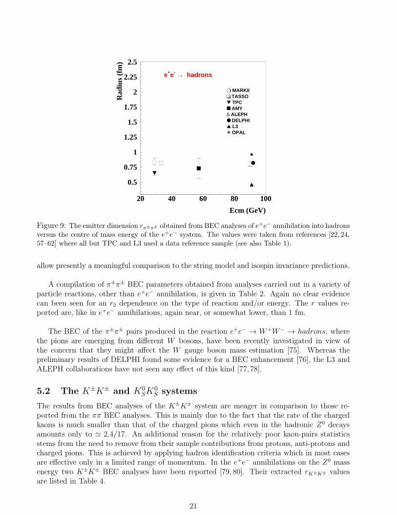
From the π±π± BEC analyses results shown in Table 1 one can make the following observa-tions. Firstly the values of r2 are in general found to be higher in the Method I analysis thanin the Method II analysis whereas the λ2 values are roughly the same. Secondly there is noclear evidence for an r dependence on the centre of mass energy. To note is also the fact thatthe values of r2 are smaller than 1 fm and their average in Method I is in the vicinity of 0.8fm. In Method II the r values are less stable and fluctuate from experiment to experiment. Itis generally believed that these fluctuations of the r values are just a reflection of the fact thatdifferent experiments used different BEC analysis procedures, namely in their data selectioncriteria and in their choice of the reference sample. This situation is also clearly seen in Fig.9 where r2 is plotted against the e+e− centre of mass energy, Ecm. In particular to note arethe three r2 values obtained in Method I for the π±π± pairs emitted from the Z0 gauge bosonwhere the OPAL value differs by several standard deviations from those reported by ALEPHand DELPHI. The L3 collaboration has not given an r value in the framework of the MethodI analysis. Unlike the abundant results on the π±π± correlations the information on the BECanalyses of π0π0 pairs is very limited due to the experimental difficulties in identifying thetwo neutral bosons. At the same time there exists an interest in the two neutral pion sys-tem both in the framework of the string model and in the so called generalised BEC whereisospin invariance is incorporated into the analysis. The two r values, obtained from the BECanalysis of the π0π0 system, present in the hadronic Z0 decay and listed in Table 1, do not

20

0.5

0.75

1

1.25

1.5

1.75

2

2.25

2.5

20 40 60 80 100

Ecm (GeV)

Rad

ius

(fm

)

e+e- → hadrons

❍ MARKII❏ TASSO▼ TPC■ AMY∆ ALEPH● DELPHI▲ L3✭ OPAL

Figure 9: The emitter dimension rπ±π± obtained from BEC analyses of e+e− annihilation into hadronsversus the centre of mass energy of the e+e− system. The values were taken from references [22, 24,57–62] where all but TPC and L3 used a data reference sample (see also Table 1).

allow presently a meaningful comparison to the string model and isospin invariance predictions.

A compilation of π±π± BEC parameters obtained from analyses carried out in a variety ofparticle reactions, other than e+e− annihilation, is given in Table 2. Again no clear evidencecan been seen for an r2 dependence on the type of reaction and/or energy. The r values re-ported are, like in e+e− annihilations, again near, or somewhat lower, than 1 fm.

The BEC of the π±π± pairs produced in the reaction e+e− → W+W− → hadrons, wherethe pions are emerging from different W bosons, have been recently investigated in view ofthe concern that they might affect the W gauge boson mass estimation [75]. Whereas thepreliminary results of DELPHI found some evidence for a BEC enhancement [76], the L3 andALEPH collaborations have not seen any effect of this kind [77, 78].

5.2 The K±K± and K0SK

0S systems

The results from BEC analyses of the K±K± system are meager in comparison to those re-ported from the ππ BEC analyses. This is mainly due to the fact that the rate of the chargedkaons is much smaller than that of the charged pions which even in the hadronic Z0 decaysamounts only to ≃ 2.4/17. An additional reason for the relatively poor kaon-pairs statisticsstems from the need to remove from their sample contributions from protons, anti-protons andcharged pions. This is achieved by applying hadron identification criteria which in most casesare effective only in a limited range of momentum. In the e+e− annihilations on the Z0 massenergy two K±K± BEC analyses have been reported [79, 80]. Their extracted rK±K± valuesare listed in Table 4.

21

Table 2: A representative sample of the two-pion emitter dimension r and the chaoticity parameter λ2

deduced from BEC studies of hadron-hadron, lepton-hadron and γγ reactions leading to multi-hadronfinal states. The data selection and reference samples, as well as the application of the Coulombcorrection, differ from experiment to experiment. In most cases the errors given are only the statisticalones. The systematic errors are typically of the order of 10 to 20% of the measured parameter values.

π±π± BEC analyses Parameter

Reaction ECM [GeV] r2 [fm] λ2

γγ → h [24] < 5 > 1.05 ± 0.08 1.20 ± 0.13

γγ → 6π± [65] 1.6 − 7.5 0.54 ± 0.22 0.59 ± 0.20

ν(ν)N → h [66] 8 − 64 0.64 ± 0.16 0.46 ± 0.16

µp→ h [67] 23 0.65 ± 0.03 0.80 ± 0.07

π+p→ h [68] 21.7 0.83 ± 0.06 0.33 ± 0.02

pp→ h [69] 26 1.02 ± 0.20 0.32 ± 0.08

pp→ h [70] 27.4 1.20 ± 0.03 0.44 ± 0.01

pp→ h [71] 63 0.82 ± 0.05 0.40 ± 0.03

pp→ h [72] 1.88 1.04 ± 0.01 1.96 ± 0.03

pp→ h [73] 200 - 900 0.73 ± 0.03 0.25 ± 0.02

e p→ e h [74] 6 < Q2γ < 100 [GeV2] 0.68 ± 0.06 0.52 ± 0.20

e p→ e h [16] 110 < Q2γ [GeV2] 0.67 ± 0.04 0.43 ± 0.09

Unlike the K±K± pairs, the origin of the K0SK

0S system is not only fed from strangeness

±2 states but also from the boson-antiboson K0K0(strangeness = 0) system which in turn

may be fed from the decay of resonances. Neglecting CP violation1 we show in the followingthat a Bose-Einstein like threshold enhancement is nevertheless expected in the Q(K0

S, K0S)

distribution even when its origin is the K0K0system [81–84].

In general a boson-antiboson, BB, pair is an eigenstate of the charge conjugation operatorC. In the absence of outside constraints, one can write the probability amplitude for a givencharge conjugation eigenvalue Cn as follows:

1√2

∣

∣

∣B;B⟩

Cn=±1=

1

2

∣

∣

∣B(p);B(−p)⟩

± 1

2

∣

∣

∣B(p);B(−p)⟩

, (34)

where p is the three momentum vector defined in the BB centre of mass system. In the Q = 0limit, where the BEC effect should be maximal, p is equal to zero and Eq. (34) reads

1√2

∣

∣

∣B;B⟩

Cn=±1=

1

2

∣

∣

∣B(0);B(0)⟩

± 1

2

∣

∣

∣B(0);B(0)⟩

. (35)

This means that, at Q = 0, the probability amplitude for the Cn = −1 state (odd ℓ values) iszero whereas the Cn = +1 state (even ℓ values) is maximal. Here it is important to note that

1The inclusion of CP violation effect in the following discussion is straightforward but with negligible conse-quences at the current experimental precision level.

22

these equations do hold for any spinless boson-antiboson pair such the K0K0, the K+K− and

the π+π− systems. What does distinguish the K0K0from the other spinless boson-antiboson

pairs is the simplicity by which one is able to project out the Cn = +1 and the Cn = −1 partsof the probability amplitude.

As is well known, the K0 and the K0mesons are described in terms of the two CP eigen-

states, K0S with CPn = +1 and K0

L with CPn = −1. From this follows that, when the K0K0

pair is detected through their K0S and K0

L decays, a definite eigenvalue Cn of the K0K0sys-

tem can be selected. Thus, as Q approaches zero, an enhancement should be observed in theprobability to detect K0

S K0S pairs and/or K0

LK0L pairs (Cn = +1), whereas a decrease should

be seen in the probability to find K0SK

0L pairs (Cn = −1). The BEC can thus be analysed by

forming for the eigenstate Cn = +1 and Cn = −1 respectively the correlation functions:

C+(Q) =2P (K0

SK0S) + 2P (K0

LK0L)

P (K0 K0)

and C−(Q) =2P (K0

SK0L) + 2P (K0

LK0S)

P (K0 K0)

, (36)

where P stands for the production rate of a given two-boson state as a function of Q.

These C+(Q) and C−(Q) dependence on Q, for λ = 1, are drawn schematically in Fig. 10.As seen, when Q approaches zero, C(Q) splits into two branches. The first rises up to the valuetwo and the other decreases to zero in such a way that their sum remains constant and equal

to one at all Q values. This means, that if all the decay modes of the K0K0pairs are detected

and used simultaneously in the same correlation analysis then, according to Eqs. (34) and (35),no BEC effect will be observed at Q = 0. This however should not come as a surprise if one

recalls that the K0K0system is at the very end not composed of two identical bosons.

Q (Arbitrary Units)

C (

Q)

Cn = +1

even wave

C n =

−1

odd

wave

0

0.2

0.4

0.6

0.8

1

1.2

1.4

1.6

1.8

2

0 0.1 0.2 0.3 0.4 0.5 0.6 0.7 0.8 0.9 1

Figure 10: Schematic behaviour of the correlation functions C(Q) of the K0 K0system given by

Eq. (36). The Cn = +1 probability amplitude reaches the value 2 at the limit of Q = 0 whereasthe Cn = −1 probability amplitude reaches the value 0. The sum of Cn = +1 and Cn = −1 remainsconstant down to Q = 0.

The interpretation of a BEC enhancement in the K0SK

0S system is not straightforward as

23

its origin may also be the decay of the scalar f0(980) resonance. This resonance, which ismainly observed in its decay to pion-pair in the decay of the Z0 gauge boson [85], lies within its

width at the K0K0threshold of 995.3 MeV. Thus the low Q enhancement seen in the K0

S K0S

correlation at Q ∼ 0 may be formed from the Bose-Einstein effect and/or from the f0(980)resonance decay. A possible method to disentangle the two contributions is given by isospinconsiderations [86] which is outlined in the following section. Values for λ and r obtained forthe K0

S K0S system, produced in e+e− annihilation on the Z0 mass, are given in Table 4.

5.3 Isospin invariance and generalised Bose-Einstein correlation

In the sector of strong interacting hadrons where BEC and FDC analyses are performed, theisospin is a conserved quantity. In analogue to the so called generalised Pauli principle, whichis the extension of that principle from two identical nucleons, the proton-proton and neutron-neutron pairs, to the proton-neutron system, one can generalise the Bose-Einstein statistics bythe inclusion of the isospin invariance. This extension may relate for example, BEC resultsof the π±π± pairs to those obtained for the π+π0 system. This extension was pointed out byseveral authors (see e.g. references [13, 87–89]) and recently was worked out in details [86] toproduce concrete relations between the BEC effects of hadron systems which are connectedby isospin and are proposed to be tested experimentally. So far however the concept of thegeneralised BEC has not been verified as it involves pion systems which include one or moreneutral pions which experimentally are hard to detect and identify. However if the gener-alised BEC assumption is confirmed then its effect on particles correlations is not negligible. Inthe following we briefly discuss some aspects of the generalised BEC features and consequences.

First to note is that in many cases boson pairs, like the KK and ππ systems, are producedtogether with other hadrons, here denoted by X , from an initial state which is isoscalar to avery good approximation. These include e.g. pairs produced from an initial multi-gluon state,pairs from hadronic decays of J/ψ and Υ, or pairs produced by Z0 decays. In some of thesecases the initial state is however not pure I=0 but has also some contamination of an I=1component which is mixed in like in those processes where the J/ψ and Υ decay to hadronsvia one photon annihilation. According to the specific case methods can be applied to reduce,or even eliminate, this contamination. For example, the subsample of the Cn = −1 quarkoniawhich decays into an odd number of pions assures, due to G-parity, that the hadronic finalstate is in an I=0 state. Forming such a subsample from the hadronic Z0 decays is not useful,but on the other hand multi-hadron final states which originate from Z0 decays into ss, cc andbb quark pairs, are in an I=0 state.

Several specific relations in the framework of the generalised Bose-Einstein statistics be-tween charge and neutral K-mesons have been proposed in reference [86]. Among others, ofa particular interest are those relations which have a bearing on the analysis of the enigmaticscalar f0(980) resonance, whose mass and width lie in the KK threshold region, and which hasa long history regarding its nature and decay modes [43, 90–92]. For details concerning theserelations the reader is advised to turn to reference [86].

Next we turn to the effect of the generalised BEC assumption on the ππ system. In thissystem there are more states and more isospin amplitudes than the two, I=0 and I=1 of theKK system. In the low Q region where only the s-wave contributes, the π+π+, π+π− and π0π0

24

amplitudes depend upon only two isospin amplitudes, I=0 and I=2. Their intensities in thisregion satisfy a triangular inequality [86]

∑

X

∣

∣

∣

∣

√

(2/3) · P [io → (π0π0)X ]−√

(1/3) · P [io → (π+π−)eX ]∣

∣

∣

∣

≤

≤∑

X

√

P [io → (π±π±)X ] =∑

X

√

P [io → (π±π0)eX ] ≤

≤∑

X

∣

∣

∣

∣

√

(2/3) · P [io → (π0π0)X ] +√

(1/3) · P [io → (π+π−)eX ]∣

∣

∣

∣

, (37)

where the notation (ππ)e is used to indicate that only even partial waves for the (ππ) final stateare included in the sum. Here io denotes an initial I=0 state and X stands for the hadronsproduced in association with the two earmarked pion-pair.

In this last relation the middle line is of a particular interest as it states that at low Qvalues, where only the s-wave survives, the BEC enhancement in the π±π0 system should beequal to that present in the π±π± pairs. Finally the BEC features of the π0π0 system shouldnot be far from that of the π+π+ state as long as the contribution of the π±π∓ to the triangleinequality relation remains small.

5.4 Observation of higher order Bose-Einstein correlations

As mentioned in Sec. 2.3, the directly measured higher order BEC are essentially limited to thecase of three identical charged pions. In these analyses, the contribution from the two-hadronBEC was subtracted in each experiment with somewhat different method. The genuine π±π±π±

BEC were also measured in the reaction e+e− → Z0 followed by an hadronic decay [93–95].The experimental normalised distribution, which is marked by (a) in Fig. 11, is that found byOPAL [94] to describe the contribution to R3(Q3), as defined in Eq. (17), from the over-allthree identical charged pion BEC enhancement. In the same figure the three-pion distribution,denoted by (b), corresponds to the BEC enhancement due to the lower order BEC correlationsi.e. the two-pion system. A clear evidence is seen for the genuine three-pion BEC enhancementwhich can be extracted by subtracting the distribution (b) from that of (a) which then allowsthe evaluation of r3.

Results for the three-boson emitter dimension are listed in Table 3 where the values of r3and the ratio r3/r2 are given. As can be seen, it does not seem to exist a significant dependenceof the r3 and r3/r2 values on the type and/or energy of the particles reaction.

In Ref. [24] a relation is derived between the two-pion emitter radius r2 and the three-pionemitter radius r3 as extracted from a fit of R3(Q3) to the over-all (non-genuine) three-bosoncorrelation distribution. This relation, which is based on the Fourier transform of a Gaussianshape hadron source, is given by the inequality

r2/√3 ≤ r3 ≤ r2/

√2 . (38)

so that r3/r2, lies in the range of 0.55 to 0.71. The inequality relation (38) is reduced to theequality

r3 = r2/√2 , (39)

25

Q3(GeV)

δ (1

04 ent

ries

/ 0.

01 G

eV)

OPAL

(a) (b)

0

1

2

3

4

5

0 0.5 1 1.5 2

Figure 11: BEC results from an OPAL study of three identical charged pions detected in the hadronicZ0 decays [94]. The over-all normalised BEC enhancement is described by the (a) distribution whereasdistribution (b) corresponds to the three-pion BEC enhancement generated from the lower order BECenhancement of the two-pion system.

when the emitter radius r3 is determined from the genuine BEC distribution parametrised byC3(Q3) so that r3/r2 should exactly be equal to 0.71. The experimental results, shown in Table3, are seen to fulfil the expected relations between r2 and r3 and in particular the results fromthe genuine three-pion correlation obtained from the hadronic Z0 decay are consistent withinone to two standard deviations with the expectation of Eq. (39).

5.5 Experimental results from Fermi-Dirac correlation analyses

Until recently FDC analyses of fermion-pairs were prohibited due to the low production rateof identical di-baryons in particle reactions at low and intermediate energies. This situationchanged with the commission of the LEP collider, operating on the Z0 mass energy, whereeach of its four experiments have accumulated some 3 to 4 million hadronic Z0 decays. Theinclusive Z0 decay branching ratio of ∼0.34 Λ per event was sufficiently high to allow a FDCanalysis of the Λ Λ(Λ Λ) and Λ Λ pairs which are free of Coulomb effects and are relatively easyidentified. Results from these analyses have been reported by the OPAL [98], DELPHI [99] andALEPH [100] collaborations using the spin-spin correlation method (see Fig. 12). The ALEPHcollaboration has further repeated its analysis with Method II, i.e. with the phase space densityapproach and found the results of both methods to be consistent within errors (see Fig. 13).In the same figure is also shown the OPAL [101] recent p p FDC measurement carried out inthe hadronic Z0 decays.

A summary of the measured di-baryon r values is given in Table 4 together with the averageLEP1 value for the π± π± pairs and values for the K± K± and K0

S K0S systems obtained from

BEC analyses. To note is the fact, as already discussed in Sec. 5.2, that the K0S K

0S pairs

may also be the decay product of resonances like the f0(980), whereas the other hadron pairslisted in the Table form, so called, exotic states, that is they are in isospin 2 or strangeness ±2

26

Table 3: Results for r3 and r3/r2 values obtained from BEC analyses of two and three identicalcharged pions. Values for genuine three-pion BEC are marked by (g) otherwise they are marked by(n).

2π and 3π BEC analyses Parameter

Reaction ECM [GeV] r3 [fm] r3/r2

π+p,K+p→ h [96] 22 0.51 ± 0.01 (g) 0.61 ± 0.12

pp→ h [97] 26 0.58 ± 0.07 (n) 0.58 ± 0.25

pp→ h [70] 27.4 0.54 ± 0.01 (n) 0.45 ± 0.07

pp→ h [71] 63 0.41 ± 0.02 (n) 0.50 ± 0.13

e+e− → h [24] 3.1 0.53 ± 0.03 (n) 0.65 ± 0.17

e+e− → γγ [24] 5 0.55 ± 0.03 (n) 0.65 ± 0.20

e+e− → h [24] 4−7 0.45 ± 0.04 (n) 0.63 ± 0.18

e+e− → h [24] 29 0.64 ± 0.06 (n) 0.77 ± 0.25

e+e− → h [58] 29−37 0.52 ± 0.07 (n) 0.59 ± 0.21

e+e− → h [93] 91 0.66 ± 0.05 (g) 0.80 ± 0.16

e+e− → h [94] 91 0.58 ± 0.05 (g) 0.73 ± 0.13

e+e− → h [95] 91 0.65 ± 0.07 (g) 1.00 ± 0.12

states or they belong to an identical di-baryon state. The most striking feature that emergesfrom the measured data listed in Table 4 is the very small r values obtained for the identicaldi-baryon systems which lie in the vicinity of ∼0.15 fm, way below the values obtained for themesons and also much smaller than the proton charge and nuclear radius [105] of ∼ 0.83±0.02fm. Finally the fact that the data in Table 4 utilised the same reaction at the same centre ofmass energy, affords a unique opportunity to study the emitter dimension r as a function ofthe hadron mass. This feature is dealt with in the following sections.

6 The r dependence on the hadron mass

The r2 dependence on the hadron mass, r(m), shown in Fig. 14, exhibits a relatively strongdecrease in r as the hadron mass increases, a feature which however currently rests mainlyon the results obtained for the baryon-pairs. The possibility that the origin of this behaviourarises from purely kinematic considerations has been explored in Ref. [106] with the conclusionthat this by itself cannot account for the rather sharp decrease of r2 with m. Thus this r2dependence on the hadron mass has to be faced by all non-perturbative QCD models whichattempt to describe the hadron production process. In particular r(m) poses a challenge to thestring approach which also constitutes a basis for the Lund model of hadronisation described indetails in [47], which expects that ∂r/∂m > 0 in its rudimental form. Whereas the somewhatsmaller value of r(mK) as compared to that of r(mπ), may still be acceptable, the very smallr2 values extracted from the Λ and proton pairs cannot apparently be accommodated withinthe Lund string approach [107].

27

0

50

100

150

200

0.0 GeV < Q < 1.5 GeV

Λ Λ , Λ−

Λ−

Ent

ries

/ 0.

2

0

500

1000

1500

2000

0.0 GeV < Q < 1.5 GeV

ΛΛ−

0

50

100

150

200

1.5 GeV < Q < 2.0 GeV0

250

500

750

1000

1.5 GeV < Q < 2.0 GeV

0

200

400

600

-1 -0.5 0 0.5 1

2.0 GeV < Q < 4.0 GeV

y

0

500

1000

1500

-1 -0.5 0 0.5 1

2.0 GeV < Q < 4.0 GeV

y

Figure 12: The ALEPH results from the spin-spin FDC analysis of the ΛΛ and ΛΛ pairs observed inthe hadronic Z0 decays [100] given at several Q regions and presented in terms of dN/dy where y isthe cosine angle between the two decay protons. The lines represent the best fit of Eq. (28) to thedata.

6.1 The r(m) description in terms of the Heisenberg relations

The maximum of the BEC and FDC effects, from which the dimension r is deduced, occurswhen the Q value of the two identical hadrons of mass m approaches zero i.e., the hadrons arealmost at rest in their CMS which also means that the three vector momentum difference ∆papproaches zero. This motivated the attempt to link the r(m) behaviour to the Heisenberguncertainty principle [102]. From these uncertainty relations one has that

∆p∆r = 2µ v r = m v r = h c , (40)

where m and v are the hadron mass and its velocity. Here µ is the reduced mass of the di-hadron system and r is the geometrical distance between them. The momentum difference ∆pis measured in GeV and r ≡ ∆r is given in Fermi units while hc = 0.197 GeV fm. From Eq.(40) follows that

r =hc

mv=

hc

p. (41)

Simultaneously one also utilises the uncertainty relation expressed in terms of time and energy

∆E∆t =p2

m∆t = h , (42)

where the ∆E is given in GeV and ∆t in seconds. Thus one has

p2 = hm/∆t so that p =√

h m/∆t . (43)

28

0

0.5

1

ALEPH

A)

C(Q

)

0

0.5

1

B)

0

0.5

1

0 1 2 3 4 5 6 7 8 9 10

Q [GeV]

C)

Q (GeV)0 1 2 3 4 5 6 7 8

C(Q

)

0

0.2

0.4

0.6

0.8

1

1.2

1.4

1.6

1.8

2

OPAL Preliminary

Figure 13: Left: The correlation function C(Q) obtained by the ALEPH collaboration [100] usingMethod II for the ΛΛ pairs for three different reference samples. A) Monte Carlo, B) and C) two,somewhat differently treated, mixed events samples. Right: The OPAL C(Q) distribution of the p psystem taken from Ref. [101]. The continuous lines represent the best fit of Eq. (29) to the C(Q)results.

Inserting this last expression for p in Eq. (41) one finally obtains

r(m) =hc/

√

h/∆t√m

=c√h∆t√m

. (44)

If one further assumes that ∆t is independent of the hadron mass and its identity and justrepresents the time scale of strong interactions, of the order of ∆t = 10−24 seconds, thenr(m) = A/

√m with A = 0.243 fm GeV1/2. This r dependence on m is shown in Fig. 14

by the thin solid line. The sensitivity of r(m) to the value of ∆t is represented by the dashedlines in the same figure. The upper and the lower dashed lines correspond respectively to thevalues of ∆t = 1.5× 10−24 and 0.5× 10−24 seconds. A fit of Eq. (44) to the data points plottedin Fig. 14 yields ∆t = (1.2 ± 0.3)× 10−24 seconds where 0.3 represents the statistical error.As seen in the figure, the dependence of r on the mass m, as determined from the Heisenbergrelations, follows within errors the measured values and thus offers a natural explanation forthe experimental found hierarchy rππ > rKK > rpp ∼ rΛΛ.

6.2 QCD description of r(m) via the virial theorem

In the previous section it has been shown that the observed hierarchy ∂r/∂m < 0 has anatural and a rather general explanation. Here we would like to demonstrate that such adependence could shed light on the character of the “soft” interaction or, in other words, onthe non-perturbative QCD which is responsible for the interaction at long distances. In thatwe follow [102] and use the semi-classical approximation as in Sec. 6.1, which means that theangular momentum is given by

ℓ = | ~p1 − ~p2 | bt = 2 p bt ≈ h c , (45)

29

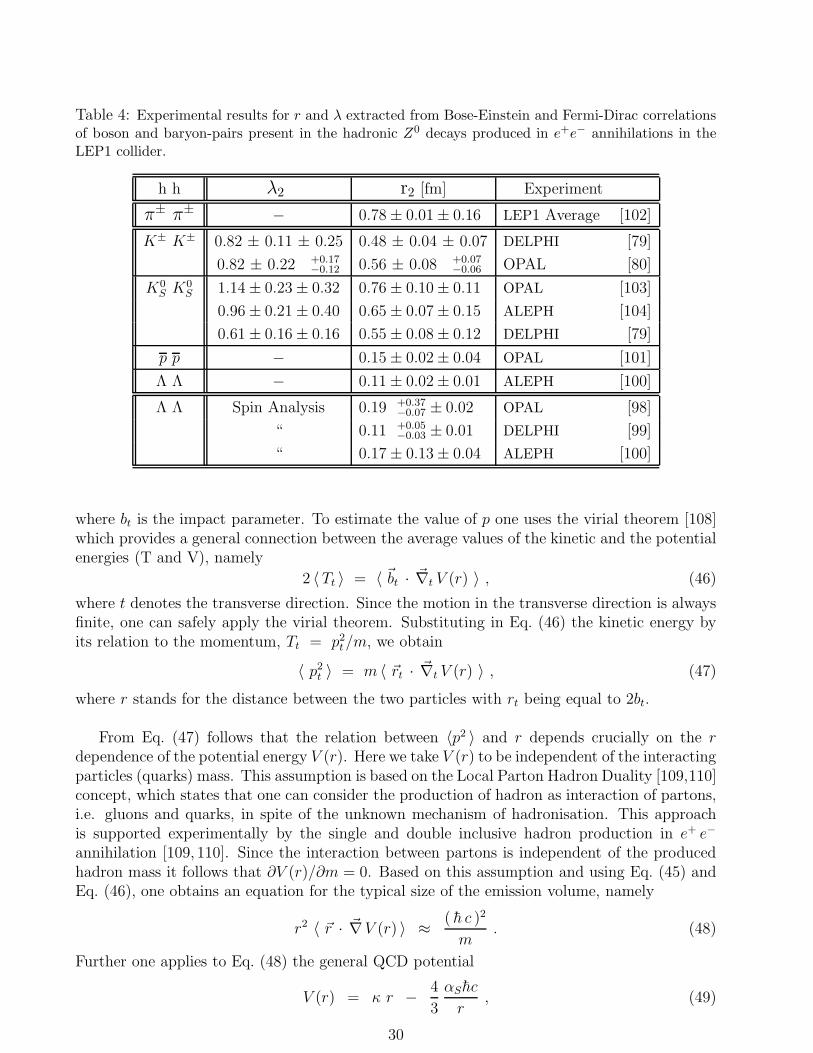
Table 4: Experimental results for r and λ extracted from Bose-Einstein and Fermi-Dirac correlationsof boson and baryon-pairs present in the hadronic Z0 decays produced in e+e− annihilations in theLEP1 collider.

h h λ2 r2 [fm] Experiment

π± π± − 0.78± 0.01± 0.16 LEP1 Average [102]

K± K± 0.82 ± 0.11 ± 0.25 0.48 ± 0.04 ± 0.07 DELPHI [79]

0.82 ± 0.22 +0.17−0.12 0.56 ± 0.08 +0.07

−0.06 OPAL [80]

K0S K

0S 1.14± 0.23± 0.32 0.76± 0.10± 0.11 OPAL [103]

0.96± 0.21± 0.40 0.65± 0.07± 0.15 ALEPH [104]

0.61± 0.16± 0.16 0.55± 0.08± 0.12 DELPHI [79]

p p − 0.15± 0.02± 0.04 OPAL [101]

Λ Λ − 0.11± 0.02± 0.01 ALEPH [100]

Λ Λ Spin Analysis 0.19 +0.37−0.07 ± 0.02 OPAL [98]

“ 0.11 +0.05−0.03 ± 0.01 DELPHI [99]

“ 0.17± 0.13± 0.04 ALEPH [100]

where bt is the impact parameter. To estimate the value of p one uses the virial theorem [108]which provides a general connection between the average values of the kinetic and the potentialenergies (T and V), namely

2 〈 Tt 〉 = 〈 ~bt · ~∇t V (r) 〉 , (46)

where t denotes the transverse direction. Since the motion in the transverse direction is alwaysfinite, one can safely apply the virial theorem. Substituting in Eq. (46) the kinetic energy byits relation to the momentum, Tt = p2t/m, we obtain

〈 p2t 〉 = m 〈 ~rt · ~∇t V (r) 〉 , (47)

where r stands for the distance between the two particles with rt being equal to 2bt.

From Eq. (47) follows that the relation between 〈p2 〉 and r depends crucially on the rdependence of the potential energy V (r). Here we take V (r) to be independent of the interactingparticles (quarks) mass. This assumption is based on the Local Parton Hadron Duality [109,110]concept, which states that one can consider the production of hadron as interaction of partons,i.e. gluons and quarks, in spite of the unknown mechanism of hadronisation. This approachis supported experimentally by the single and double inclusive hadron production in e+ e−

annihilation [109, 110]. Since the interaction between partons is independent of the producedhadron mass it follows that ∂V (r)/∂m = 0. Based on this assumption and using Eq. (45) andEq. (46), one obtains an equation for the typical size of the emission volume, namely

r2 〈 ~r · ~∇V (r) 〉 ≈ ( h c )2

m. (48)

Further one applies to Eq. (48) the general QCD potential

V (r) = κ r − 4

3

αShc

r, (49)

30

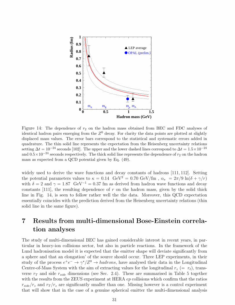
Hadron mass (GeV)

Rad

ius

(fm

)

▲ LEP average

● OPAL (prelim.)

mp mΛmπ mK0

0.1

0.2

0.3

0.4

0.5

0.6

0.7

0.8

0.9

1

0 0.5 1 1.5

Figure 14: The dependence of r2 on the hadron mass obtained from BEC and FDC analyses ofidentical hadron pairs emerging from the Z0 decay. For clarity the data points are plotted at slightlydisplaced mass values. The error bars correspond to the statistical and systematic errors added inquadrature. The thin solid line represents the expectation from the Heisenberg uncertainty relationssetting ∆t = 10−24 seconds [102]. The upper and the lower dashed lines correspond to ∆t = 1.5×10−24

and 0.5×10−24 seconds respectively. The thick solid line represents the dependence of r2 on the hadronmass as expected from a QCD potential given by Eq. (49).

widely used to derive the wave functions and decay constants of hadrons [111, 112]. Settingthe potential parameters values to κ = 0.14 GeV2 = 0.70 GeV/fm , αs = 2π/9 ln(δ + γ/r)with δ = 2 and γ = 1.87 GeV−1 = 0.37 fm as derived from hadron wave functions and decayconstants [111], the resulting dependence of r on the hadron mass, given by the solid thickline in Fig. 14, is seen to follow rather well the the data. Moreover, this QCD expectationessentially coincides with the prediction derived from the Heisenberg uncertainty relations (thinsolid line in the same figure).

7 Results from multi-dimensional Bose-Einstein correla-

tion analyses

The study of multi-dimensional BEC has gained considerable interest in recent years, in par-ticular in heavy-ion collisions sector, but also in particle reactions. In the framework of theLund hadronisation model it is expected that the emitter shape will deviate significantly froma sphere and that an elongation’ of the source should occur. Three LEP experiments, in theirstudy of the process e+e− → γ⋆/Z0 → hadrons, have analysed their data in the LongitudinalCentre-of-Mass System with the aim of extracting values for the longitudinal rz (= rℓ), trans-verse rT and side rside dimensions (see Sec. 2.4). These are summarised in Table 5 togetherwith the results from the ZEUS experiment at HERA ep collisions which confirm that the ratiosrside/rz and rT/rz are significantly smaller than one. Missing however is a control experimentthat will show that in the case of a genuine spherical emitter the multi-dimensional analysis

31

procedure will in fact yield the results that rside/rz ≈ rT/rz ≈ 1.

A somewhat surprising result which came out of the BEC multi-dimensional analysis ofpion-pairs is the dependence of rz, as well as rside and rT , on the transverse mass mT . Anexample of this rz dependence on mT is the one reported by the DELPHI collaboration [113]which is shown in Fig. 15. This rz(mT ) behaviour is very similar to that seen in heavy ioncollisions where it is often attributed to nuclei collective effects which should be absent inparticle reactions and in particular in e+e− annihilations. A theoretical understanding in termsof the Lund model of this effect in particle reactions is apparently still lacking even if only forthe reason that the inclusion of the BEC effect into the model is a highly non-trivial task andstill seems to need further improvements [114, 115].

Table 5: Evidence for the elongation of the source from experimental results for the ratios rside/rzand rT /rz obtained from multi-dimensional BEC analyses of identical charged pions. The first andthe second errors are respectively the statistical and systematic ones.

Reaction√s [GeV] Experiment rside/rz rT/rz

e+e− → Z →h 91 L3 [37] 0.80± 0.02+0.03−0.18

e+e− → Z →h 91 OPAL [39] 0.82± 0.02+0.01−0.05

e+e− → Z →h 91 DELPHI [38] 0.62± 0.02± 0.05

e p→ e h 110 < Q2γ [GeV2] ZEUS [16] 0.67± 0.08

7.1 rz(mT) description in terms of the Heisenberg relations

We have seen that there is a a great similarity between the dependence of the 1-dimensional r2on the hadron mass m and the dependence of the rz on the transverse mass mT . This is notsurprising once one realises that the longitudinal distance ∆rz, and ∆pz, the difference in thelongitudinal momentum of the two hadrons in the LCMS, are also conjugate observables whichobey the uncertainty relation [116]

∆rz∆pz = hc . (50)

Here ∆pz is measured in GeV, ∆rz ≡ rz is given in Fermi units and hc = 0.197 GeV fm. Inthe LCMS one has

∆pz = 2µvz = pz ,

where µ = m/2 is the reduced mass of the two identical hadrons of massm and the longitudinalvelocity vz of these hadrons. Thus

rz =hc

pz. (51)

Simultaneously one considers the uncertainty relation expressed in terms of energy and time

∆E∆t = h , (52)

32

0.2

0.3

0.4

0.5

0.6

0.7

0.8

0.9

0 0.5 1 1.5mT

ππ (GeV)

r z (fm

)

∆t = 2.1x10-24sec

∆t = 1.0x10-24sec

Figure 15: Preliminary results of DELPHI [113] for the dependence of the longitudinal emitterdimension rz(ππ) on the transverse mass mT (ππ) in hadronic Z0 decays. The data are compared withthe expression for rz given in Eq. (59) setting ∆t to the best fitted value of 2.1 ×10−24 sec (continuousline) and the expectation for 1.0 ×10−24 sec (dashed line).

where ∆E is given in GeV and ∆t in seconds. In as much as the total energy E of the two-hadron system is given by their mass and their kinetic energy, i.e. the potential energy can beneglected, one has

E =2∑

i=1

√

m2 + p2i,x + p2i,y + p2z =2∑

i=1

√

m2i,T + p2z , (53)

where m1,T and m2,T are the transverse mass of the first and second hadron. As Qz decreasesthe longitudinal momentum pz vanishes so that one can, once p2z < m2

i,T , expand the hadronenergy E in terms of p2z/m

2i,T and retain only the two first terms,

E =2∑

i=1

mi,T

√

√

√

√1 +p2zm2

i,T

≈2∑

i=1

mi,T +2∑

i=1

1

2

p2zmi,T

. (54)

Next one can order the identical bosons so that m1,T ≥ m2,T and define

δmT =m1,T −m2,T

m2T − (δmT )2

while mT =m1,T +m2,T

2. (55)

Inserting these relations into Eq. (54) one gets, after a few algebraic steps that

E = 2mT +mT p

2z

m2T − (δmT )2

. (56)

Thus as long as m2T ≫ (δmT )

2 the total energy of the di-boson system is approximately equalto

E ≈ 2mT +p2zmT

. (57)

33

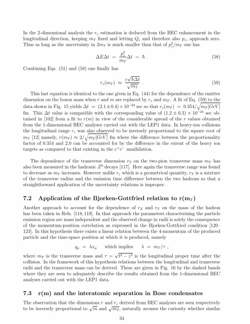
In the 2-dimensional analysis the rz estimation is deduced from the BEC enhancement in thelongitudinal direction, keeping mT fixed and letting Qz and therefore also pz, approach zero.Thus as long as the uncertainty in 2mT is much smaller than that of p2z/mT one has

∆E∆t =p2zmT

∆t = h . (58)

Combining Eqs. (51) and (58) one finally has

rz(mT ) ≈ c√h∆t√mT

. (59)

This last equation is identical to the one given in Eq. (44) for the dependence of the emitterdimension on the boson mass when r and m are replaced by rz and mT . A fit of Eq. (59) to the

data shown in Fig. 15 yields ∆t = (2.1±0.4)×10−24 sec so that rz(mT ) = 0.354/√

mT [GeV ]

fm. This ∆t value is compatible with the corresponding value of (1.2 ± 0.3) × 10−24 sec ob-tained in [102] from a fit to r(m) in view of the considerable spread of the r values obtainedfrom the 1-dimensional BEC analyses carried out with the LEP1 data. In heavy-ion collisionsthe longitudinal range rz was also observed to be inversely proportional to the square root of

mT [12] namely, r(mT ) ≈ 2/√

mT [GeV ] fm where the difference between the proportionalityfactor of 0.354 and 2.0 can be accounted for by the difference in the extent of the heavy iontargets as compared to that existing in the e+e− annihilation.

The dependence of the transverse dimension rT on the two-pion transverse mass mT hasalso been measured in the hadronic Z0 decays [117]. Here again the transverse range was foundto decrease as mT increases. However unlike rz which is a geometrical quantity, rT is a mixtureof the transverse radius and the emission time difference between the two hadrons so that astraightforward application of the uncertainty relations is improper.

7.2 Application of the Bjorken-Gottfried relation to r(mT )

Another approach to account for the dependence of rZ and rT on the mass of the hadronhas been taken in Refs. [118, 119]. In that approach the parameters characterising the particleemission region are mass independent and the observed change in radii is solely the consequenceof the momentum-position correlation as expressed in the Bjorken-Gottfried condition [120–123]. In this hypothesis there exists a linear relation between the 4-momentum of the producedparticle and the time-space position at which it is produced, namely

qµ = λxµ which implies λ = mT/τ ,

where mT is the transverse mass and τ =√t2 − z2 is the longitudinal proper time after the

collision. In the framework of this hypothesis relations between the longitudinal and transverseradii and the transverse mass can be derived. These are given in Fig. 16 by the dashed bandswhere they are seen to adequately describe the results obtained from the 1-dimensional BECanalyses carried out with the LEP1 data.

7.3 r(m) and the interatomic separation in Bose condensates

The observation that the dimensions r and rz derived from BEC analyses are seen respectivelyto be inversely proportional to

√m and

√mT , naturally arouses the curiosity whether similar

34

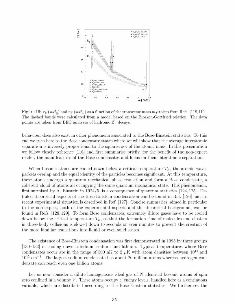
Mass Dependen e of HBT Correlations in e

+

e

�

Annihilation (II) 2907

0

0.2

0.4

0.6

0.8

1

0 0.2 0.4 0.6 0.8 1 1.2m [ GeV ]

R [

fm

]

R||

R⊥

R0 (K,Λ0) ALEPHR0 (K,Λ0) DELPHIR0 (K,Λ0) OPAL

R⊥ (π) DELPHIR|| (π) DELPHIR⊥ =Rtside (π) L3R|| (π) L3R⊥ =Rtside (π) OPALR|| (π) OPAL

Fig. 1. R

k

and R

?

al ulated from the model (shaded bands) for �;K; p;�. Data

points atm = m

�

represent results of 2- and 3-dimensional analysis of LEP data [4℄.

For 3-dim results the R

Tside

was hosen as the representative geometri al transverse

dimension of the pions sour e. Points at higher masses represent 1-dim sour e

radius R

0

[5℄

4. In on lusion, we have found that the orrelation between the mo-

mentum and the produ tion point of a produ ed hadron, suggested by the

Gottfried�Bjorken hypothesis of the in-out as ade, seems to a ount for

the observed orrelation between identi al parti les observed in e

+

e

�

an-

nihilation. In parti ular, it an a ount for the experimentally measured

anisotropy of the two-pion orrelation fun tion. The mass dependen e of

the �sour e radius� is also adequately des ribed. Large un ertainties, both

in the theoreti al determination of the model parameters, and in the experi-

mental data do not allow, however, to obtain more quantitative on lusions.

Several omments are in order.

(i) The mass dependen e of the e�e tive HBT orrelation radii al ulated

from the model and shown in Fig. 1 was obtained under the assumption

that the parameters of the model do not depend on parti le masses.

For v; Æ and � this assumption an be � in prin iple � veri�ed,

on e better data are available. No su h dire t he k is in sight for

�

0

, however. Nevertheless, sin e the observed mass dependen e of the

Figure 16: rz (=R||) and rT (=R⊥) as a function of the transverse massmT taken from Refs. [118,119].The dashed bands were calculated from a model based on the Bjorken-Gottfried relation. The datapoints are taken from BEC analyses of hadronic Z0 decays.

behaviour does also exist in other phenomena associated to the Bose-Einstein statistics. To thisend we turn here to the Bose condensate states where we will show that the average interatomicseparation is inversely proportional to the square-root of the atomic mass. In this presentationwe follow closely reference [116] and first summarise briefly, for the benefit of the non-expertreader, the main features of the Bose condensates and focus on their interatomic separation.

When bosonic atoms are cooled down below a critical temperature TB, the atomic wave-packets overlap and the equal identity of the particles becomes significant. At this temperature,these atoms undergo a quantum mechanical phase transition and form a Bose condensate, acoherent cloud of atoms all occupying the same quantum mechanical state. This phenomenon,first surmised by A. Einstein in 1924/5, is a consequence of quantum statistics [124, 125]. De-tailed theoretical aspects of the Bose-Einstein condensation can be found in Ref. [126] and itsrecent experimental situation is described in Ref. [127]. Concise summaries, aimed in particularto the non-expert, both of the experimental aspects and the theoretical background, can befound in Refs. [128, 129]. To form Bose condensates, extremely dilute gases have to be cooleddown below the critical temperature TB, so that the formation time of molecules and clustersin three-body collisions is slowed down to seconds or even minutes to prevent the creation ofthe more familiar transitions into liquid or even solid states.

The existence of Bose-Einstein condensation was first demonstrated in 1995 by three groups[130–132] in cooling down rubidium, sodium and lithium. Typical temperatures where Bosecondensates occur are in the range of 500 nK to 2 µK with atom densities between 1014 and1015 cm−3. The largest sodium condensate has about 20 million atoms whereas hydrogen con-densate can reach even one billion atoms.

Let us now consider a dilute homogeneous ideal gas of N identical bosonic atoms of spinzero confined in a volume V . These atoms occupy ǫi energy levels, handled here as a continuousvariable, which are distributed according to the Bose-Einstein statistics. We further set the

35

ground state to be ǫ0 = 0. If N0 is the number of atoms in this ground state and Nex is thenumber of atoms in the excited states then N = N0 + Nex. For a homogeneous ideal gas ofidentical bosonic atoms it can be shown (see e.g. Ref. [133]) that at a low temperature T onehas

Nex = 2.612 V

(

2πmkT

h2

)3/2

, (60)

where V is the volume occupied by the atoms of massm. Since TB is defined as the temperaturewhere almost all bosons are still in excited states, we can, to a good approximation, equate Nwith Nex. That is

N = 2.612 V

(

2πmkTBh2

)3/2

. (61)

For T < TB one obtains from Eqs. (60) and (61) that the number of atoms N0 which are inthe condensate state is,

N0 = N −Nex = N

[

1−(

T

TB

)3/2]

, (62)

where T is the temperature of the atoms lying at the excited energy states above the condensateenergy level ǫ0 = 0. The atomic density of the Bose gas at very low temperatures, T/TB << 1where N ≈ N0, is then given by

ρ =N

V= 2.612

(

2πmkT

h2

)3/2

, (63)

where k is the Boltzmann constant and ρ, the atomic density, has the dimension of L−3. Fromthis follows that ρ−1/3 is the average interatomic separation in the Bose condensate. At thesame time the thermal de Broglie wave length is equal to

λdB =

(

h2

2πmkT

)1/2

. (64)

Combining Eqs. (63) and (64) one has for the state of a Bose condensate the relation

ρλ3dB ≈ 2.612 . (65)

Thus the average interatomic distance in a Bose condensate, dBE , is equal to

dBE ≡ ρ−1/3 ≈ λdB/1.378 . (66)

Next one can consider two different bosonic gases, having atoms with masses m1 and m2,which are cooled down to the same very low temperature T0, below the critical temperature TBof both of them. In this case one produces two Bose condensates with interatomic distances

dBE(mi) ≈√2π

1.378

(

h2

mikT0

)1/2

; i = 1, 2 . (67)

From this follows that when two condensates are at the same fixed temperature T0 one has

dBE(m1)

dBE(m2)=

√

m2

m1

, (68)

36

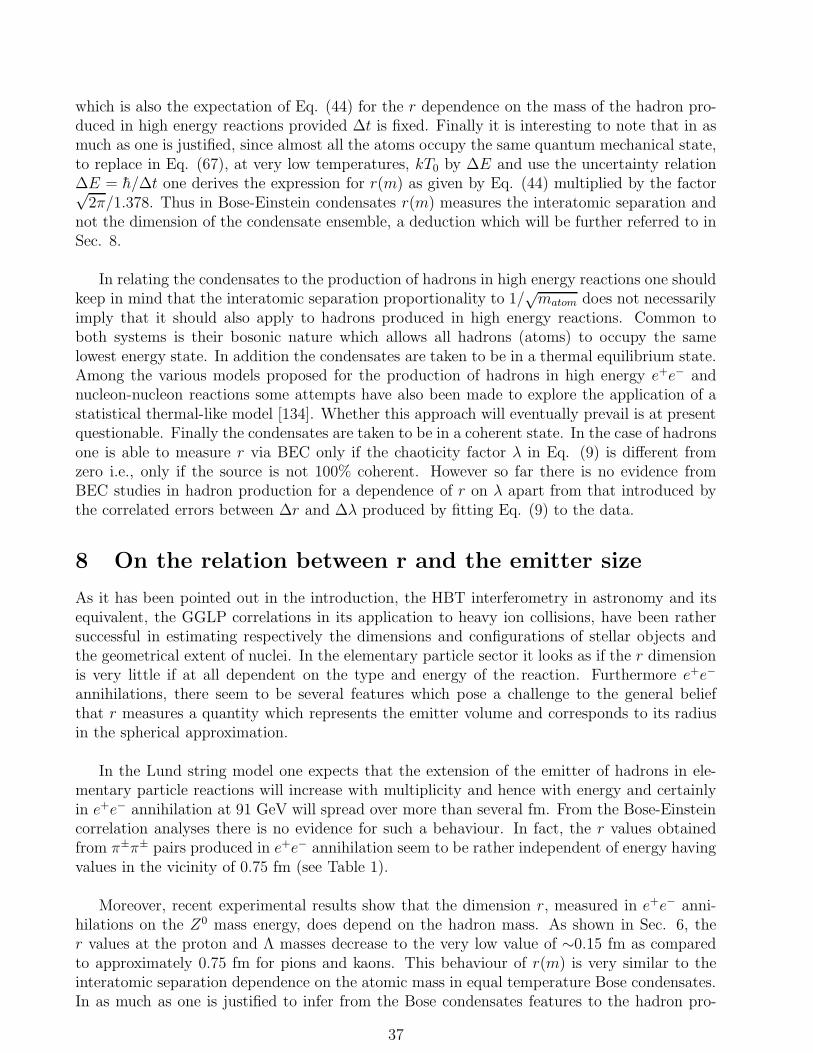
which is also the expectation of Eq. (44) for the r dependence on the mass of the hadron pro-duced in high energy reactions provided ∆t is fixed. Finally it is interesting to note that in asmuch as one is justified, since almost all the atoms occupy the same quantum mechanical state,to replace in Eq. (67), at very low temperatures, kT0 by ∆E and use the uncertainty relation∆E = h/∆t one derives the expression for r(m) as given by Eq. (44) multiplied by the factor√2π/1.378. Thus in Bose-Einstein condensates r(m) measures the interatomic separation and

not the dimension of the condensate ensemble, a deduction which will be further referred to inSec. 8.

In relating the condensates to the production of hadrons in high energy reactions one shouldkeep in mind that the interatomic separation proportionality to 1/

√matom does not necessarily

imply that it should also apply to hadrons produced in high energy reactions. Common toboth systems is their bosonic nature which allows all hadrons (atoms) to occupy the samelowest energy state. In addition the condensates are taken to be in a thermal equilibrium state.Among the various models proposed for the production of hadrons in high energy e+e− andnucleon-nucleon reactions some attempts have also been made to explore the application of astatistical thermal-like model [134]. Whether this approach will eventually prevail is at presentquestionable. Finally the condensates are taken to be in a coherent state. In the case of hadronsone is able to measure r via BEC only if the chaoticity factor λ in Eq. (9) is different fromzero i.e., only if the source is not 100% coherent. However so far there is no evidence fromBEC studies in hadron production for a dependence of r on λ apart from that introduced bythe correlated errors between ∆r and ∆λ produced by fitting Eq. (9) to the data.

8 On the relation between r and the emitter size

As it has been pointed out in the introduction, the HBT interferometry in astronomy and itsequivalent, the GGLP correlations in its application to heavy ion collisions, have been rathersuccessful in estimating respectively the dimensions and configurations of stellar objects andthe geometrical extent of nuclei. In the elementary particle sector it looks as if the r dimensionis very little if at all dependent on the type and energy of the reaction. Furthermore e+e−

annihilations, there seem to be several features which pose a challenge to the general beliefthat r measures a quantity which represents the emitter volume and corresponds to its radiusin the spherical approximation.

In the Lund string model one expects that the extension of the emitter of hadrons in ele-mentary particle reactions will increase with multiplicity and hence with energy and certainlyin e+e− annihilation at 91 GeV will spread over more than several fm. From the Bose-Einsteincorrelation analyses there is no evidence for such a behaviour. In fact, the r values obtainedfrom π±π± pairs produced in e+e− annihilation seem to be rather independent of energy havingvalues in the vicinity of 0.75 fm (see Table 1).

Moreover, recent experimental results show that the dimension r, measured in e+e− anni-hilations on the Z0 mass energy, does depend on the hadron mass. As shown in Sec. 6, ther values at the proton and Λ masses decrease to the very low value of ∼0.15 fm as comparedto approximately 0.75 fm for pions and kaons. This behaviour of r(m) is very similar to theinteratomic separation dependence on the atomic mass in equal temperature Bose condensates.In as much as one is justified to infer from the Bose condensates features to the hadron pro-

37

duction sector, r(m) apparently does not measure the emitter radius but rather the distancebetween two neighbouring identical hadrons.

In any case, the experimental results found for the dependence of r on the hadron mass arenot reconcilable with the notion of a unique emitter radius for all outgoing hadrons. Howeverthe possibility that baryons are emitted from a much smaller source than pions and kaons hasits own difficulty [135] if one considers the source energy density ǫ. To illustrate this problemlet us assume that the emitter source is a sphere of radius r, as determined from the correlationanalysis, filled homogeneously with at least the energy which corresponds to the sum of therest masses of the two outgoing identical hadrons. Then, for a given hadron mass mh and itsemitter radius rh, the energy density of the source is given by

ǫmeasured =3

4π

2mh

r3h(69)

which is plotted in Fig. 17 for the pion, kaon, proton and Λ pairs. The dashed lines in thefigure are the predicted dependence of the energy density on the hadron mass computed fromEq. (70), which is based on the expression of r(m) given in Eq. 44, namely

ǫmodel =3

2π

m5/2h

c3(h∆t)3/2. (70)

Whereas the energy density of the pion and kaon pairs are still lying within an acceptable range,the energy density of the proton and Λ emitter sources reach the very high value of about 100GeV/fm3.

10-1

1

10

10 2

0 1 2 32 mh (GeV)

Ede

nsit

y(G

eV/f

m3 )

▲ LEP average● OPAL (prelim.)

Figure 17: Energy density of the hadron emitter, calculated from Eq. (69), as a function of thehadron mass assuming a spherical emitter having the radius r which was extracted from the BECanalysis. The dashed lines are the expectations from Eq. (70) setting ∆t to plus and minus threestandard deviations away from its median value of 1.2× 10−24 seconds [135].

In trying to cope with these observations, it may be helpful to try and identify the un-derlying variable or variables, apart from the hadron mass, which r depends on. A partial

38

answer to this quest [136], which is briefly outlined in the following section, is provided by therelation between the BEC analysis and the genuine particle correlation method which utilisesthe factorial cumulant moments (see Sec. 2.3).

8.1 The r dependence on the number of emitting sources

Let us consider a simplified description of heavy ions (AA) interactions at high energies whichis given in terms of several distinct, say S, primary nucleon-nucleon (nn) collisions leading tohadrons. In this approach the hadrons produced in a single primary nucleon-nucleon reactionare emitted from an Snn source. The hadron produced in heavy ion (AA) collisions are thencoming from SAA sources so that SAA/Snn=S. Since here the AA collisions are described interms of the single primary nucleon-nucleon reactions one can define, without loss of generality,Snn as a unit source so that SAA = S.

Next the π±π± pairs emerging from a single primary nucleon-nucleon reaction and thoseemerging from the heavy ion collisions are subject to BEC analyses and the correlation functions

CS=12 (Q) = 1 + λS=1e

−Q2r2S=1 and CS

2 (Q) = 1 + λSe−Q2r2

S

are fitted, each to its corresponding data distribution. In general for every S value the resultingrS can be extracted from the fitted correlation functions by integration C2 − 1 over Q fromzero to infinity so that

∫ ∞

0

[

CS2 (Q)− 1

]

dQ =∫ ∞

0λSe

−Q2r2SdQ =

1

2

λS√π

rS, (71)

where λS is, as customary in the BEC analyses, taken to be independent of Q.

For the two-particle correlation there exists a relation (see e.g. Ref. [137]) between thecumulant K2 and the BEC function C2, namely that

C2(Q) = 1 + λe−r2Q2

= 1 + K2 . (72)

In addition it has been shown [138–140] that for two particle correlation the cumulant KS2 of S

sources is, to a very good approximation, related to the value of the corresponding cumulantof one source, KS=1

2 , byKS

2 = KS=12 /S .

Thus the BEC function CS2 is equal to

CS2 (Q) = 1 + λSe

−r2SQ2

= 1 +KS=1

2

S= 1 +

λS=1e−r2

S=1Q2

S. (73)

By integrating Eq. (73) over Q from zero to infinity one finally obtains that

rS = SλSλS=1

rS=1 , (74)

where S like the λ parameters is taken to be independent of Q. Consequently if the increaseof an emitter volume is coupled to an increase in the number of boson sources, then the BECextracted rS will grow as well. Further to note is that if in heavy-ion collisions SλS/λS=1 is

39

proportional to A1/3 then r will be proportional to the nucleus radius. As for the HBT analysisapplied in astronomy, the proportionality between the stellar object dimension and the numberof photon sources is self-evident.

From the discussion above it is obvious that the choice of the unit source determines thepredicted dependence of r on the various features, such as type and energy, of the hadron (orphoton) emitting reaction. In the case of heavy ion collisions the choice of the unit source tobe a single primary nucleon-nucleon collision is a natural one. In the case of e+e− annihilationone may consider the possibility that See itself is the unit source. Under this assumption thenumber of sources does not change with energy and r will remain constant. This predictionseems to be consistent with the measured r values allowing for the fact that the various ex-periments used different analysis methods and reference samples (see Sec. 5.1). On the otherhand an increase of r as a function of the hadron multiplicity has been observed in the BECanalysis [22] of equally non-zero charged pion-pairs emerging from the Z0 decay. Furthermorethe same experiment also found that the extracted r value from the Z0 decays into three hadronjets was by about 10% higher than that obtained from the Z0 decay events having only twohadron jets. Similar rise of r with the average hadron multiplicity has also been reported byseveral hadron-hadron collision experiments carried out at centre of mass energies above 30GeV [73, 141–143].

These last findings indicate that apparently for the e+e− annihilations a reasonable choicefor the unit source is the single hadron jet. The shortcoming of such a choice is however thefact that the charge multiplicity of a hadron jet depends on its energy and on its origin, i.e. if itis a quark or a gluon [144–146], which currently impedes a detailed quantitative prediction forthe behaviour of r as a function of the centre of mass energy and the multiplicity. Regardlessof these hindrances, the adaptation of the hadron jet as a unit source provides nevertheless aqualitative explanation for the increase of r with multiplicity and also expects in e+e− annihi-lations a moderate dependence of r on the e+e− centre of mass energy.

9 Summary and conclusions

The 1-dimensional Bose-Einstein correlation enhancement measured in identical pion-pairs closein time-phase space, is found to be a universal phenomenon present in a large variety of parti-cle reactions and over a wide range of energies. Nevertheless, there are still missing systematicBEC studies concentrating on the same reaction at different energies, and/or different reactionsat the same energy, which will allow a comprehensive investigation of the dependence of r onthe variables that characterise the particle interactions. Notwithstanding the fact that thesesystematic studies are still missing and that BEC analyses cannot currently be considered asprecision measurements, the extracted r values, which are taken to represent the hadron emit-ter source, seem to be very little, if at all, dependent on the reaction type or on its energy andthey are seen to fluctuate in the range of about 0.6 to 1.0 fm.

The essentially constant r value seems to be in contradiction with the results obtainedfrom the BEC studies of heavy-ion collisions and from the HBT analyses of stellar objects.An insight into the origin of this difference is offered by the relation between the BEC andthe cumulant moments analysis where the introduction of the so called hadron source plays a

40

central role. From this relation follows that the value of r is proportional to the number ofactive hadron sources which participate in the reaction. In particle reactions the proposal toequate the number of sources with the number of hadron jets offers an understanding of ther dependence on multiplicity. At the same time however the difficulty in defining a standardhadron jet prohibits presently any quantitative results.

The genuine higher order BEC analyses are presently restricted to three identical chargedpions. Assuming a Gaussian hadron emitter, the expected relation r2/

√3 ≤ r3 ≤ r2/

√2 be-

tween the two and three-pion BEC dimension parameters, is found to be consistent withinerrors with the measurements carried out in e+e− annihilation and hadron collisions. Thedirect measurement of the genuine correlations of four and more pion systems has not beenrealised so far. On the other hand the extracted r values from the , so to speak, non-genuinecorrelations, are model dependent and as such less reliable.

Recently first results from 2 and 3-dimensional BEC analyses of pion-pairs have been re-ported. These verified the Lund string model expectation that the hadron emitter sourcedeviates from a sphere and is elongated in the thrust (or sphericity) direction of the multi-hadron final state. In the approximation that the emitter has an elongated prolate ellipsoidshape, where the long axis rℓ is in the thrust direction and rT is the axis perpendicular to it,the ratio rT/rℓ is found be in the range of ∼0.7 to ∼0.8.

The extension of the BEC analysis to the fermion sector was shown to be feasible via thePauli exclusion principle. First results from the so called Fermi-Dirac correlation analysis ofthe ΛΛ and proton−proton pairs, emerging from the hadronic Z0 decays, have demonstratedthat the dimension r is strongly dependent on the mass of the identical hadrons. It has beenfurther shown that this dependence can be accounted for by the Heisenberg uncertainty rela-tions, or alternatively by QCD derived potential, to yield the relation r(m) ∝ 1/

√m. Similar

relation is seen to be valid also in the 2-dimensional BEC analysis when r is replaced by the rℓand m by the transverse mass mt. It is interesting further to note that the interatomic sepa-ration in the Bose condensates having the same low temperature, is proportional to 1/

√matom .

So far the FDC analyses were restricted to the Z0 hadronic decays, therefore it is essentialthat they will be repeated in other particle reactions to verify that indeed r of the Λ and theproton pairs is in the vicinity of 0.15 fm. This small r value, derived from the FDC analysesof baryon-pairs, poses a challenge to the concept that r represents the hadron emitter radius.If one does insist on keeping the radius emitter interpretation for r then one encounters thesituation of an unreasonable high energy density value, of some 100 GeV/fm3, of the baryonssource. Thus the very small rΛΛ and rpp values indicate that our level of understanding theproduction of hadrons, and in particular baryons, is apparently far from being satisfactory.

Acknowledgements

I would like to express my thanks to my colleagues G. Bella, I. Cohen, E.K. Grinbaum-Sarkisyan, P. Soding, and E. Tsur for many helpful discussions and comments. I am in particularindebted to B. Ilan for going diligently over the manuscript to ensure that it is free of errorsand omissions.

41

References

[1] R. Hanbury-Brown and R. Q. Twiss. Phil. Mag., 45:663, 1954.

[2] R. Hanbury-Brown and R. Q. Twiss. Nature, 177:27, 1956.

[3] R. Hanbury-Brown and R. Q. Twiss. Nature, 178:1046, 1956.

[4] D. H. Boal, C. K. Gelbke, and B. K. Jenning. Rev. Mod. Phys., 62:553, 1990.

[5] G. Baym. Acta Phys. Polon., B29:1839, 1998.

[6] U. A. Wiedemann and U. Heinz. Phys. Rept., 319:145, 1999.

[7] G. Goldhaber et al. Phys. Rev. Lett., 3:181, 1959.

[8] G. Goldhaber et al. Phys. Rev. Lett., 120:300, 1960.

[9] G. Alexander and H. J. Lipkin. Phys. Lett., B352:162, 1995.

[10] A. D. Chacon et al. Phys. Rev., C43:2670, 1991, and references therein.

[11] U. Heinz. Hanbury-Brown Twiss interferometry for relativistic heavy ion collisions: theo-retical aspects. In Proc. of Int. Summer School on Correlations and Clustering Phenom-ena in Subatomic Physics, page 137, Dronten, The Netherlands, 1996.

[12] U. Heinz and B.V. Jacak. Ann. Rev. Nucl. Part. Sci., 49:529, 1999, and references therein.

[13] R. M. Weiner. Phys. Rept., 327:249, 2000.

[14] M. Ringner. Correlations in multiparticle production. PhD thesis, Lund University, Lund,Sweden, 1998.

[15] OPAL collaboration, P. D. Acton, et al. Phys. Lett., B267:143, 1991.

[16] ZEUS collaboration, M. Derrick. Acta Phys. Polon., B33:3281, 2002.

[17] T. Osada, S. Sano, and M. Biyajima. Z. Phys., C72:285, 1996.

[18] G. I. Kopylov and M. I. Podgoretskii. Sov. J. Nucl. Phys., 15:219, 1972.

[19] G. I. Kopylov and M. I. Podgoretskii. Sov. J. Nucl. Phys., 18:336, 1973.

[20] G. I. Kopylov. Phys. Lett., B50:472, 1974.

[21] W Hofmann. A fresh look at Bose-Einstein correlations. Research Note LBL-23108,Lawrence Berkeley Laboratory, UC, 1987.

[22] OPAL collaboration, G. Alexander, et al. Z. Phys., C72:389, 1996.

[23] E. A. De Wolf, I. M. Dremin, and W. Kittel. Phys. Rept., 270:1, 1996.

[24] MARK II collaboration, I. Juricic, et al. Phys. Rev., D39:1, 1989.

[25] M. Biyajima et al. Prog. Theor. Phys., 84:931, 1990.

42

[26] UA1-MINIMUM BIAS collaboration, N. Neumeister, et al. Phys. Lett., B275:186, 1992.

[27] P. Carruthers and I. Sarcevic. Phys. Rev. Lett., 63:1562, 1989.

[28] E. A. De Wolf. Acta Phys. Pol., B21:611, 1990.

[29] R. J. Barlow. Statistics. John Wiley & and Sons., 1989.

[30] T. Csorgo and S. Pratt. Structure of the peak in Bose-Einstein correlation. In T. Csorgoet al., editors, Proc. of the Workshop on relativistic heavy ion physics, page 75, Budapest,Hungary, 17-21 June 1991.

[31] K. Geiger et al. Phys. Rev., D61:054002, 2000.

[32] DELPHI collaboration, P. Abreu, et al. Phys. Lett., B471:460, 2000.

[33] NA44 collaboration, H. Beker, et al. Phys. Rev. Lett, 74:3340, 1995.

[34] NA35 collaboration, T. Alber, et al. Z. Phys., C66:77, 1995.

[35] EHS/NA22 collaboration, N. M. Agababyan, et al. Z. Phys., C66:409, 1995.

[36] EHS/NA22 collaboration, N. M. Agababyan, et al. Z. Phys., C71:405, 1996.

[37] L3 collaboration, M. Acciarri, et al. Phys. Lett., B458:517, 1999.

[38] DELPHI collaboration, P. Abreu, et al. Phys. Lett., B471:460, 2000.

[39] OPAL collaboration, G. Abbiendi, et al. Eur. Phys. J., C16:423, 2000.

[40] B. Andersson and M. Ringner. Nucl. Phys., B513:627, 1998.

[41] B. Andersson and M. Ringner. Phys. Lett., B421:283, 1998.

[42] E. Segre. Nuclei and Particles. Benjamin/Cummings Publishing Co., 2nd edition, 1982.

[43] Particle Data Group, K. Hagiwara, et al. Phys. Rev., D66:1, 2002.

[44] E. P. Wigner. Z. Phys., 43:624, 1927.

[45] C. Eckart. Rev. Mod. Phys., 2:305, 1930.

[46] R. Lednicky. On correlation and spin composition techniques. Research Note PhE-10,MPI, 1999.

[47] B. Andersson et al. Phys. Rep., 97:31, 1983.

[48] B. R Webber. Nucl. Phys., B238:492, 1984.

[49] B. Andersson and M. Ringner. Nucl. Phys., B513:627, 1998.

[50] M. Gyulassy et al. Phys. Rev., C20:2267, 1979.

[51] M. G. Bowler. Phys. Lett., B270:69, 1991.

[52] M. Biyajima et al. Phys. Lett., B353:340, 1995.

43

[53] E. Tsur. Bose-Einstein correlations of three charged pions in hadronic Z0 decays. Master’sthesis, Tel-Aviv University, Tel-Aviv, Israel, 1997.

[54] Y. M. Liu et al. Phys. Rev., C34:1667, 1986.

[55] J. G. Cramer. Phys. Rev., C43:2798, 1991.

[56] E. O. Alt et al. Eur. Phys. J., C13:663, 2000.

[57] TPC collaboration, H. Aihara, et al. Phys. Rev., D31:996, 1985.

[58] TASSO collaboration, M. Althoff, et al. Z. Phys., C30:355, 1986.

[59] AMY collaboration, S. K. Choi, et al. Phys. Lett., D355:406, 1995.

[60] ALEPH collaboration, D. Decamp, et al. Z. Phys., C54:75, 1992.

[61] DELPHI collaboration, P. Abreu, et al. Phys. Lett., B286:201, 1992.

[62] L3 collaboration, P. Achard, et al. Phys. Lett., B524:55, 2002.

[63] M. Sanders. Pion (non-) correlations in hadronic events at the Z resonance. PhD thesis,The Nijmegen Catholic University, The Netherlands, 2002.

[64] OPAL Collaboration, Physics Note PN-513, 2002. Submitted to the XXXII Int. Symp.on Multiparticle Dynamics (ISMD), 7-13 September 2002, Alushta, Ukraine.

[65] CELLO collaboration, H. J. Behrend, et al. Phys. Lett., B245:298, 1990.

[66] Big Bubble Chamber Neutrino collaboration, V. A. Korotkov, et al. Z. Phys., C60:37,1993.

[67] EMC collaboration, M. Arneodo et al. Z. Phys., C32:1, 1986.

[68] NA22 collaboration, M. Adamus, et a. Z. Phys., C37:347, 1988.

[69] NA23 collaboration, J. L. Bailly, et al. Z. Phys., C43:431, 1989.

[70] NA27 collaboration, M. Aguilar-Benitez, et al. Z. Phys., C54:21, 1992.

[71] AFS collaboration, T. Akesson, et al. Z. Phys., C36:517, 1987.

[72] CPLEAR collaboration, R. Adler, et al. Z. Phys., C63:541, 1994.

[73] UA1 collaboration, C. Albajar, et al. Phys. Lett., B226:410, 1989.

[74] H1 collaboration, C. Adloff, et al. Z. Phys., C75:437, 1997.

[75] The LEP collaborations, ALEPH, DELPHI, L3, OPAL, and the LEPWW working group.CERN EP preprint, 2003.

[76] DELPHI collaboration, N. van Remortel, et al. In Proc. of Int. Symp. on MultiparticleDynamics, Alushta, Ukraine, 7-13 September 2002.

[77] L3 collaboration, P. Achard, et al. Phys. Lett., B547:139, 2002.

44

[78] ALEPH collaboration, R. Barate, et al. Phys. Lett., B478:50, 2000.

[79] DELPHI collaboration, P. Abreu, et al. Phys. Lett., B379:330, 1996.

[80] OPAL collaboration, G. Abbiendi, et al. Euro. Phys. J., C21:23, 2001.

[81] H. J. Lipkin. Phys. Lett., B219:474, 1989.

[82] H. J. Lipkin, Argonne National Laboratory priprint ANL-HEP-PR-88-66, 1988.

[83] H. J. Lipkin. Phys. Rev. Lett., 69:3700, 1992.

[84] G. Alexander. Bose-Einstein effect in the K0 K0in boson-antiboson system. Research

Note 93/001, LNF, 1993.

[85] DELPHI collaboration, P. Abreu, et al. Phys. Lett., B298:236, 1993.

[86] G. Alexander and H. J. Lipkin. Phys. Lett., B456:270, 1999.

[87] M. Biyajima et al. Phys. Rev., C58:2316, 1998.

[88] M. Suzuki. Phys. Rev., D35:3359, 1987.

[89] M. G. Bowler. Phys. Lett., B197:443, 1987.

[90] D. Morgan and M. R. Pennington. Phys. Lett., B258:44, 1991.

[91] D. Morgan and M. R. Pennington. Phys. Rev., D48:1185, 1993.

[92] F. E. Close et al. Phys. Lett., B319:291, 1993.

[93] DELPHI collaboration, P. Abreu, et al. Phys. Lett., B355:415, 1995.

[94] OPAL collaboration, K. Ackerstaff, et al. Eur. Phys. J., C5:239, 1998.

[95] L3 collaboration, P. Achard, et al. Phys. Lett., B540:185, 2002.

[96] EHS/NA22 collaboration, N. M. Agababian, et al. Z. Phys., C68:229, 1995.

[97] NA23 collaboration, J. L. Bailly, et al. Z. Physik, C43:341, 1989.

[98] OPAL collaboration, G. Alexander, et al. Phys. Lett., B384:377, 1996.

[99] DELPHI collaboration, T. Lesiak and H. Palka. Determination of the spin compositionof ΛΛ and ΛΛ (ΛΛ) pairs in hadronic Z decays (DELPHI 98-114 CONF 176). In Proc.of the XXIX Int. Conf. on High Energy Physics, Vancouver, Canada, 22-29 July 1998.

[100] ALEPH collaboration, R. Barate, et al. Phys. Lett., B475:395, 2000.

[101] OPAL Collaboration, Physics Note PN486, 2002. Submitted to the Int. Conf. on HighEnergy Physics (HEP 2001) 12-18 July 2001, Budapest, Hungary.

[102] G. Alexander, I. Cohen, and E. Levin. Phys. Lett., B452:159, 1999.

[103] OPAL collaboration, R. Akers, et al. Z. Phys., C67:389, 1995.

45

[104] ALEPH collaboration, D. Buskulic, et al. Z. Phys., C64:361, 1994.

[105] SELEX collaboration, I. Eschrich, et al. Phys. Lett., B522:233, 2001.

[106] M. Smith. Phys. Lett., B477:141, 2000.

[107] B. Andersson. Some theory remarks on Bose-Einstein correlation. In Proc. of the XXVthLes Rencontres de Moriond, Les Arcs, France, 18-20 March 2000.

[108] C. Cohen-Tannoudji, B. Diu, and F. Laloe. Quantum Mechanics. John Wiley and Sonspublishing Co., 1990.

[109] Ya. Asimov et al. Z. Phys., C31:213, 1986, and references therein.

[110] V. A. Khoze and W. Ochs. Int. J. Mod. Phys., A12:2949, 1997, and references therein.

[111] M. R. Ahmady, R. R. Mendel, and J. D. Talman. Phys. Rev., D55:419, 1997, and refer-ences therein.

[112] B. Blok and M. Lublinsky. Phys. Rev., D57:2676, 1998, and references therein.

[113] B. Lorstad and O.G. Smirnova. Transverse mass dependence of Bose-Einstein correlationradii in e+e− annihilation at LEP energies. In Proc. 7th Int. Workshop on MultiparticleProduction: Correlations and Fluctuations, page 42, Nijmegen, The Netherland, 1997.World Scientific Publishing Co.

[114] O. Smirnova. Nucl. Phys. (Proc. Suppl.), B92:301, 2001.

[115] S. Todorova-Nova. Bose-Einstein correlations at LEP and HERA. In Proc. of the XXXIInt. Conf. on High Energy Physics, Amsterdam, 24-31 July 2002.

[116] G. Alexander. Phys. Lett., B506:45, 2001.

[117] L3 collaboration,. Study of Bose-Einstein correlations in Z decays at LEP. In Proc. XXIXInt. Conf. on HEP, Vancouver, 1998.

[118] A. Bialas et al. Phys. Rev., D62:114007, 2000.

[119] A. Bialas et al. Acta Phys. Polon., B32:2901, 2001.

[120] K. Gottfried. Phys. Rev. Lett., 32:957, 1974.

[121] F. E. Low and K. Gottfried. Phys. Rev., D17:2487, 1978.

[122] J. D. Bjorken. Phys. Rev., D27:140, 1983.

[123] J. D. Bjorken. Phys. Rev., D7:282, 1973.

[124] A. Einstein. Sitszber. Kgl. Preuss. Akad. Wiss. rep. 261, 1924.

[125] A. Einstein. Sitszber. Kgl. Preuss. Akad. Wiss. rep. 3, 1925.

[126] F. Dalfovo et al. Rev. Mod. Phys., 71:463, 1999, and references therein.

46

[127] See e.g. the Georgia Southern University BEC bibliography on the web athttp:// amo.phy.gasou.edu/bec.html/bibliography.html.

[128] W. Ketterle. Physics Today, 52(12):30, 1999.

[129] K. Burnett, M. Edwards, and C. Clark. Physics Today, 52(12):37, 1999.

[130] M. H. Anderson et al. Science, 269:198, 1995.

[131] K. B. Davis et al. Phys. Rev. Lett., 75:3969, 1995.

[132] C. C. Bradley et al. Phys. Rev. Lett., 75:1687, 1995.

[133] D. H. Trevena. Statistical Mechanics − An Introduction. Prentice-Hall/Ellis Horwood,1993.

[134] F. Becattini, L. Bellucci, and G. Passaleva. Transverse momentum spectra of identifiedparticles in high energy collisions with statistical hadronisation model. In A. Giovanniniand R. Ugoccioni, editors, Proc. IX Int. Workshop on Multiparticle Production, page 363,Torino, Italy, 12-17 June 2000, and references therein. Nucl. Phys. B (Suppl.) 92 (2001)363.

[135] G. Alexander, Emitter size as a function of mass and transverse mass, hep-ph/0108194,In Proceedings of the EPS International Conference on High Energy Physics, Budapest,2001 (D. Horvath, P. Levai, A. Patkos, eds.), JHEP (http://jhep.sissa.it/), ProceedingsSection, PrHEP-hep2001/027.

[136] G. Alexander and E. K. G. Sarkisyan. To be published.

[137] J. G. Cramer and K. Kadija. Phys. Rev., C53:908, 1996.

[138] P. Lipa and B. Bushbeck. Phys. Lett., B223:465, 1989.

[139] B. Bushbeck, H. C. Eggers, and P. Lipa. Phys. Lett., B481:187, 2000.

[140] G. Alexander and E. K. G. Sarkisyan. Phys. Lett., B487:215, 2000.

[141] AFS collaboration, T. Akesson, et al. Phys. Lett., B129:269, 1983.

[142] AFS collaboration, T. Akesson, et al. Phys. Lett., B187:420, 1987.

[143] SFM collaboration, A. Breakstone, et al. Z. Phys., C33:333, 1987.

[144] I. M. Dremin and J. W. Gary. Phys. Lett., B459:341, 1999.

[145] A. Capella et al. Phys. Rev., D61:074009, 2000.

[146] M. Boutemeur. Fortschr. Phys., 50:1001, 2002.

47