Elements of the wave-particle duality of light

Borys Jagielski

Thesis submitted for the degree of

Master of Science

in Physics

University of Oslo

May 2009

Abstract

The following Master’s thesis is concerned with several aspects of the wave-particle duality of light.

It is loosely divided in three parts. In the first part we consider historical, theoretical and experimental

aspects of the duality problem. We explain how the notion of duality has developed through the last 400

years. We discuss theoretical underpinnings of the duality emodied by Maxwell’s electromagnetic theory,

quantization of electromagnetic modes, Fock’s states and coherent states. We critically review several

experiments which serve to demonstrate the corpuscular or undulatory behaviour of light and matter;

in particular we present how the photoelectric effect and the Compton effect can be explained using the

undulatory model, and we critically review Grangier, Roger and Aspect correlation experiment.

In the second part we describe two illustrative experiments on the duality of light conducted at

Quantum Optics Laboratory at University of Oslo. The results of the experiment allow us to discuss

how coincidence measurements can be used to exhibit the corpuscular behaviour of light, and how Mach-

Zender interferometry performed at very low intensity can be used to exhibit the undulatory behaviour at

the (assumed) single-photon level. In addition, in the second part we review elements of theories closely

associated with the experiment and the experimental setup: optical coherence, photocount and photon

statistics, beam splitter models and Gaussian beams. A proposition for extending the semiclassical model

is given, and shortcomings of the present beam splitter models are discussed.

In the third part of the thesis we consider first Afshar’s experiment and some of the critical response

that it has been met with. Then we discuss how the wave-particle duality is to be understood in the

standard interpretation of quantum mechanics, and how it could possibly be explained using either an

alternative model for light or an alternative interpretation of quantum mechanics, and what difficulties

such explanations present.

The thesis has been written in LATEX using the graphical program LYX. The figures not reproducedfrom original sources have been generated using Matlab or drawn using Dia.

Contents

Acknowledgments iii

Introduction v

1 The historical development of the wave-particle duality concept 11.1 The 1600s and the birth of modern optics . . . . . . . . . . . . . . . . . . . . . . . . . . . . . 21.2 1800s and the triumph of the wave theory of light . . . . . . . . . . . . . . . . . . . . . . . . . 71.3 The early 1900s and the rise of quantum mechanics . . . . . . . . . . . . . . . . . . . . . . . . 11

2 The classical and the quantum descriptions of light 172.1 Maxwell’s electromagnetical theory . . . . . . . . . . . . . . . . . . . . . . . . . . . . . . . . . 172.2 The review of the quantum harmonic oscillator formalism . . . . . . . . . . . . . . . . . . . . 202.3 Quantization of the electromagnetic modes . . . . . . . . . . . . . . . . . . . . . . . . . . . . 22

2.3.1 The electromagnetic potentials . . . . . . . . . . . . . . . . . . . . . . . . . . . . . . . 222.3.2 Expansion in electromagnetic modes . . . . . . . . . . . . . . . . . . . . . . . . . . . . 242.3.3 The photon number states . . . . . . . . . . . . . . . . . . . . . . . . . . . . . . . . . . 252.3.4 Some problematic aspects of the quantized theory . . . . . . . . . . . . . . . . . . . . 27

2.4 The coherent states . . . . . . . . . . . . . . . . . . . . . . . . . . . . . . . . . . . . . . . . . . 29

3 Experimental considerations of the wave-particle duality 313.1 The black-body radiation . . . . . . . . . . . . . . . . . . . . . . . . . . . . . . . . . . . . . . 323.2 Interference (Michelson interferometry) . . . . . . . . . . . . . . . . . . . . . . . . . . . . . . . 333.3 The photoelectric effect . . . . . . . . . . . . . . . . . . . . . . . . . . . . . . . . . . . . . . . 403.4 The Compton effect . . . . . . . . . . . . . . . . . . . . . . . . . . . . . . . . . . . . . . . . . 463.5 The photon anticoincidence effect . . . . . . . . . . . . . . . . . . . . . . . . . . . . . . . . . . 51

4 Classical description of optical coherence and correlations 574.1 The complex analytic signal . . . . . . . . . . . . . . . . . . . . . . . . . . . . . . . . . . . . . 574.2 Describing optical coherence . . . . . . . . . . . . . . . . . . . . . . . . . . . . . . . . . . . . . 604.3 Quantifying optical coherence . . . . . . . . . . . . . . . . . . . . . . . . . . . . . . . . . . . . 674.4 Application to interferometry . . . . . . . . . . . . . . . . . . . . . . . . . . . . . . . . . . . . 74

5 The main elements of the experimental setup: theoretical review 775.1 Photodetector . . . . . . . . . . . . . . . . . . . . . . . . . . . . . . . . . . . . . . . . . . . . . 78

5.1.1 Types of photodetectors . . . . . . . . . . . . . . . . . . . . . . . . . . . . . . . . . . . 785.1.2 The semiclassical model . . . . . . . . . . . . . . . . . . . . . . . . . . . . . . . . . . . 795.1.3 The corpuscular model . . . . . . . . . . . . . . . . . . . . . . . . . . . . . . . . . . . . 835.1.4 Concluding remarks . . . . . . . . . . . . . . . . . . . . . . . . . . . . . . . . . . . . . 87

5.2 Beam splitter . . . . . . . . . . . . . . . . . . . . . . . . . . . . . . . . . . . . . . . . . . . . . 895.2.1 The classical description . . . . . . . . . . . . . . . . . . . . . . . . . . . . . . . . . . . 895.2.2 The quantum model . . . . . . . . . . . . . . . . . . . . . . . . . . . . . . . . . . . . . 925.2.3 Shortcomings of the beam splitter model . . . . . . . . . . . . . . . . . . . . . . . . . . 95

5.3 The shape of the laser beam . . . . . . . . . . . . . . . . . . . . . . . . . . . . . . . . . . . . . 985.3.1 The paraxial Helmholtz equation . . . . . . . . . . . . . . . . . . . . . . . . . . . . . . 995.3.2 The Gaussian beam . . . . . . . . . . . . . . . . . . . . . . . . . . . . . . . . . . . . . 1005.3.3 The ABCD law . . . . . . . . . . . . . . . . . . . . . . . . . . . . . . . . . . . . . . . . 103

6 The main elements of the experimental setup: specifications and preliminary measure-ments 1056.1 Modelling the laser beam shape . . . . . . . . . . . . . . . . . . . . . . . . . . . . . . . . . . . 1056.2 Measuring the coherence length . . . . . . . . . . . . . . . . . . . . . . . . . . . . . . . . . . . 1096.3 Specifications of the beam splitter model . . . . . . . . . . . . . . . . . . . . . . . . . . . . . . 111

i

6.4 The single-photon counting module . . . . . . . . . . . . . . . . . . . . . . . . . . . . . . . . . 1126.5 Measuring the photocount statistics . . . . . . . . . . . . . . . . . . . . . . . . . . . . . . . . 116

7 An experimental illustration of wave-particle duality 1197.1 The coincidence measurements . . . . . . . . . . . . . . . . . . . . . . . . . . . . . . . . . . . 120

7.1.1 Description . . . . . . . . . . . . . . . . . . . . . . . . . . . . . . . . . . . . . . . . . . 1207.1.2 Setup and discussion of photocount rates . . . . . . . . . . . . . . . . . . . . . . . . . 1207.1.3 Results . . . . . . . . . . . . . . . . . . . . . . . . . . . . . . . . . . . . . . . . . . . . 1237.1.4 Analysis and comparison with numerical simulations . . . . . . . . . . . . . . . . . . . 1237.1.5 Conclusion . . . . . . . . . . . . . . . . . . . . . . . . . . . . . . . . . . . . . . . . . . 126

7.2 The Mach-Zender interferometry . . . . . . . . . . . . . . . . . . . . . . . . . . . . . . . . . . 1297.2.1 Description . . . . . . . . . . . . . . . . . . . . . . . . . . . . . . . . . . . . . . . . . . 1297.2.2 Setup . . . . . . . . . . . . . . . . . . . . . . . . . . . . . . . . . . . . . . . . . . . . . 1297.2.3 Results and analysis . . . . . . . . . . . . . . . . . . . . . . . . . . . . . . . . . . . . . 1307.2.4 Conclusion . . . . . . . . . . . . . . . . . . . . . . . . . . . . . . . . . . . . . . . . . . 133

8 The Afshar experiment 1358.1 Description and results . . . . . . . . . . . . . . . . . . . . . . . . . . . . . . . . . . . . . . . . 1358.2 Criticism of the experiment . . . . . . . . . . . . . . . . . . . . . . . . . . . . . . . . . . . . . 1388.3 Concluding remarks . . . . . . . . . . . . . . . . . . . . . . . . . . . . . . . . . . . . . . . . . 139

9 Explaining the wave-particle duality 1439.1 The “photon clump” model . . . . . . . . . . . . . . . . . . . . . . . . . . . . . . . . . . . . . 143

9.1.1 Basic assumptions . . . . . . . . . . . . . . . . . . . . . . . . . . . . . . . . . . . . . . 1439.1.2 Quantitative considerations . . . . . . . . . . . . . . . . . . . . . . . . . . . . . . . . . 1459.1.3 Concluding remarks . . . . . . . . . . . . . . . . . . . . . . . . . . . . . . . . . . . . . 147

9.2 Complementarity of the Copenhagen interpretation . . . . . . . . . . . . . . . . . . . . . . . . 1489.3 The Bohmian interpretation of quantum mechanics . . . . . . . . . . . . . . . . . . . . . . . . 151

9.3.1 Reformulating the Schrödinger equation . . . . . . . . . . . . . . . . . . . . . . . . . . 1529.3.2 The nature of the quantum field . . . . . . . . . . . . . . . . . . . . . . . . . . . . . . 1569.3.3 Interpretation of electromagnetic field . . . . . . . . . . . . . . . . . . . . . . . . . . . 1589.3.4 Concluding remarks . . . . . . . . . . . . . . . . . . . . . . . . . . . . . . . . . . . . . 159

10 Conclusion 16110.1 Summary and outlooks . . . . . . . . . . . . . . . . . . . . . . . . . . . . . . . . . . . . . . . . 16110.2 Closing words . . . . . . . . . . . . . . . . . . . . . . . . . . . . . . . . . . . . . . . . . . . . . 164

A The formalism of quantum mechanics 167

B Demonstration of properties of the coherent states 173B.1 The minimal uncertainty . . . . . . . . . . . . . . . . . . . . . . . . . . . . . . . . . . . . . . . 173B.2 The time evolution of a coherent state . . . . . . . . . . . . . . . . . . . . . . . . . . . . . . . 174B.3 The coherent states as a basis . . . . . . . . . . . . . . . . . . . . . . . . . . . . . . . . . . . . 175

C Matter waves 179

D Numerical routines 183D.1 Simulation of thermal emission . . . . . . . . . . . . . . . . . . . . . . . . . . . . . . . . . . . 183D.2 Simulation of coincidence measurements . . . . . . . . . . . . . . . . . . . . . . . . . . . . . . 184

References 189

ii

Acknowledgments

First and foremost I would like to thank my thesis advisor, Arnt Inge Vistnes. His critical remarks regarding

the wave-particle duality inspired me to dedicate my thesis to this highly interesting and problematic subject;

and then, during the writing process, his patient help, both with theoretical questions and practical difficulties

encountered at the laboratory, was truly invaluable. Thank you, Arnt Inge.

Furthermore, I wish to thank Arnt Inge Vistnes, Joakim Bergli, Håkon Brox, Johanne Lein and

Eimund Smestad for our informal discussions regarding Afshar’s experiment, coincidence measurements

and quantum mechanics in general.

I want also to thank Stanislaw Krawczyk, Michal Klosowski and Bartosz Porebski for reading

some chapters of the thesis prior to the publication and providing apt comments regarding both the content

and the lingual side. Of course, any remaining mistakes and obscurities are solely due to my negligence.

My thanks go to Efim Brondz who had constructed several electronic and photodetecting devices that

I employed when conducting my measurements.

Finally, I thank Joar Bølstad for introducing me to the program LYX with which the thesis was written.

Working with LYX is definitely much more fun than using LATEX in plain-text format.

iii

iv

Introduction

I remember quite well my first exposure to quantum mechanics. It occured during the early high school years

through a Polish edition of the book The Large, the Small and the Human Mind written by Roger Penrose

[1]. In accordance with the title, Penrose dedicated the middle part of his rather short book to the issues

concerning the microscopic world. It was a fascinating reading but not a very easy one, despite the book

being labeled as popular science. If I could today advice my younger self, probably I would propose another,

more accessible introduction to the quantum branch of science. On the other hand... maybe I would not,

because getting thrown into intellectual deep water sometimes may act stimulating, and, after all, Penrose’s

book did not subdue my interest for physics.

One often hears that the quantum phenomena are against our common sense and stand in sharp contra-

diction to our day-to-day perception of the world. However, this opinion is usually uttered by professionals

in the field who have had enough time to grow accustomed to different aspects of quantum mechanics. Even

on me, after barely six years of studying physics, the paradoxes and the strange ontology of the microscopic

realm do not make as huge an impression as they once did. But when I was reading The Large, the Small

and the Human Mind, my reactions were very different indeed. The superposition principle as applied to

the quantum states, saying that an object may possess two mutually exclusive properties, struck me with

amazement. The wave-particle duality, illustrated in a standard way by the double-slit experiment, seemed

hard to grasp. And after reading the chapter about quantum entanglement and the EPR paradox I naively

assumed that the author had meant in fact something else and that I did not understand correctly what he

had been saying. It was simply too weird.

The wave-particle duality is one of the central concepts of quantum mechanics, but the discussion on

the nature of light is much older than the physical discipline initiated by Max Planck’s famous lecture in

December 1900. Let us briefly notice that the general notion of duality (or dualism) alone has also a long and

interesting history, and has always stood for crucial philosophical contrasts and problems. The relationship

between matter and mind is arguably the most famous of these, and René Descartes was the first philosopher

who considered it in depth. Descartes maintained that mind ought to be viewed as a non-physical substance.

This so-called Cartesian dualism initiated modern philosophy of mind which up to the present day ponders

the problem of the interactions between mind and body. Among other dualisms, there is the famous concept

due to Plato who postulated that our mundane world is accompanied by the world of eternal ideas; and

Immanuel Kant’s distinction between the empiricial knowledge and the noumena that are independent of the

senses [2].

The duality that will concern us here, the wave-particle duality, evolved from the dispute over the nature

v

of visible light that had started already in the times of Isaac Newton when the modern physics was being

born. However, it was quantum mechanics that radically changed the character of the debate by saying that

the structure of matter is exactly as ambiguous as that of light, and then by claiming that the way out of the

wave-or-particle stalemate is to take the dualistic stance – light and matter behave sometimes like particles,

and sometimes like waves, depending on (experimental) circumstances. Such a solution still causes unrest

among some physicists, but the general majority of the scientific society just take for granted the following

short definition of the wave-particle duality given by dictionaries:

“[t]he phenomenon where electromagnetic radiation and particles can exhibit either wave-like

or particle-like behaviour, but not both.” [3]

The famous double-slit experiment, different versions of which we will come back to in the course of the

thesis, serves as the canonical illustration of the wave-particle duality. Let us here present its simplified

description: A light beam emerges from a source, propagates through two very small slits and impinges on

a screen. We can reduce the intensity of the beam in such a way that according to a standard concept of

quantum mechanics there will be only one quantum of light (photon) present in the apparatus at any given

time. If we now place a detector behind each slit, we will see that they do not respond simultaneously, and

thus we will be led to the conclusion that the photons behave like tiny corpuscles moving through either the

first or the second slit. However, if we choose not to disturb the light with measurement before it reaches

the screen, an interference pattern will emerge on it. This pattern is most easily predicted and explained by

claiming that light is in fact an electromagnetic wave. The double-slit experiment can be also conducted with

electrons (or other material particles) instead of light, and the same conclusions would be reached. In the

words of Richard Feynman, this extraordinary phenomenon “is impossible, absolutely impossible, to explain

in any classical way, and (...) has in it the heart of quantum mechanics. In reality, it contains the only

mystery” [4]. Thus, claimed Feynman, the wave-particle duality problem is one of the central features of

quantum mechanics.

Even though the problem of the wave-particle duality is in principle as much about light as about mat-

ter, in practice an asymmetry sneaks in and a tendency to favour light often occurs. The main reason is a

technological one – it is easier to probe the properties of light and to make it exhibit undulatory or corpus-

cular behaviour, than to conduct experiments where matter behaves in a wavelike fashion. The double-slit

experiment with electrons remained a thought experiment through the large part of the 20th century, and it

was performed in a precise way in a laboratory as late as in 1989 [5]. On the other hand, the invention of

laser in the early 1960s [6] invited the scientists to explore the fundamental properties of light and paved the

way for a new branch of physical science: quantum optics.

The author has chosen to accept this asymmetry fully and dedicate the thesis to the wave-particle duality

of light. This is partly due to the fact that his experiments conducted at Quantum Optics Laboratory at

University of Oslo are concerned with light, and partly due to the fact that (in his opinion) the wave-particle

duality of light seems more interesting than the duality of matter. However, since a complete exclusion of the

duality of matter from the treatment would be inappropriate, it has been succinctly described in Appendix

C.

Two important remarks must be made at this point. In the whole thesis the word “light” will serve as a

synonym for “electromagnetic radiation” although in literature “light” means usually the visible part of the

vi

electromagnetic spectrum lying approximately between 400 and 800 nm. We will rather use the explicit term

“visible light” every time we want to refer to the latter. On the other hand we should notice that almost any

discussion of corpuscular properties of light is in practice restricted to the region lying around the visible

part of the spectrum and below it (in the sense of even shorter wavelengths), even though the idea of photon

should principially apply to the whole spectrum. We will follow this somewhat problematic practice in the

course of our thesis, but we will comment on it in Section 2.3.4.

Secondly, we want to keep apart the photonic hypothesis (saying that the electromagnetic field consists

of corpuscular entitites called photons) and the quantization hypothesis (saying that at the microscopic level

many properties of physical systems change discretely with energy being probably the most important one).

The concept of photon will be critically analyzed in the thesis, but the general quantization hypothesis will

never be challenged. The difference between these two will be also examined closer in Section 2.3.4.

After these remarks, we are now ready to present the goal of the thesis: to describe, examine and

critically analyze several aspects of the wave-particle duality of light. More specifically we intend

to:

• present the wave-particle duality from the historical, the theoretical and the experimental point of

view. Particularly, in the latter case, we aim at giving a critical review of some experiments commonly

associated with the corpuscular nature of light.

• describe different photodetection models in connection with experiments conducted by the author at

Quantum Optics Laboratory. These experiments will serve as an illustration of the wave-particle

duality of light, and their analysis will reveal that it is in fact easier to unambiguously demonstrate the

undulatory properties of light than the corpuscular properties.

• discuss whether and how the wave-particle duality could be possibly explained in the context of Afshar’s

experiment, an alternative model of light and an alternative interpretation of quantum mechanics.

There can be no doubt that the totality of the wave-particle duality problem is a very complex and rich

subject, in the sense that one may consider it from many different angles and initiate an in-depth discussion

of any single aspect of it. Unfortunately, there is no room for all that in a Master’s thesis, and this is why

the title of the work begins with “Elements of” – some elements were included, but then other elements had

to be left out. Particularly:

• We will avoid any considerations of quantum electrodynamics (QED). This may seem as a very large

omission, but we will see that a lot of interesting issues related to the wave-particle duality may be

consistently discussed outside the framework of QED. The author does not doubt that through careful

analysis of quantum electrodynamics many important insights would be gained, but entering the realm

of quantum field theories in addition to everything else would be simply too big a task.

• We will refrain from relating the wave-particle duality explicitly to the measurement problem of quan-

tum mechanics and to the collapse of the wave function, although this issue will be briefly touched upon

in Chapter 9.2 when discussing the standard interpretation of quantum mechanics. However, in our

discussion we will omit altogether decoherence phenomena, quantum nonlocality and Bell’s theorem.

vii

• In our discussion of nonclassical states of light in Chapters 4 and 5.1 we examine both antibunched light

and sub-Poissonian light, but the third main instance of nonclassical light, so-called squeezed states, is

left out.

We believe that despite any necessary omissions we will still manage to give a coherent – although definitely

not exhausting – treatise on the subject of the wave-particle duality of light.

The thesis is loosely divided into three parts which correspond to our aforementioned intentions. The

first part describes the fundamental historical, theoretical and experimental ingredients of the wave-particle

duality of light. Chapter 1 is strictly historical, and follows in a non-mathematical fashion the development

of the wave-or-particle question from the 17th till the 20th century. The “real” physics does not begin

until Chapter 2, where we depict two standard, but very different physical models of light, the classical

electromagnetical one postulating light waves, and the quantum-mechanical one postulating photons (to be

understood either as light corpuscles or as quanta of radiative energy). These contradictory models represent

the theoretical essence of the wave-particle duality in the case of electromagnetic radiation. The first part

of the thesis ends with Chapter 3 where we inspect critically what the empirical side of physics has to say

on the dual nature of light and matter. We describe interferometry experiments suggesting that radiation

possesses a wave nature, and we review experiments which seem to ascribe corpuscular properties to light.

The second part of the thesis describes an experiment performed on laser light at Quantum Optics Labo-

ratory (QOL) at the University of Oslo. Utilizing two different experimental setups, one with single-photon

detectors measuring a split beam in coincidence, and another employing a Mach-Zender interferometer, we

try to give an experimental illustration of the duality of light, and we carefully discuss the results. All this

does not come before Chapter 7, with Chapters 4, 5 and 6 preparing grounds for the experiment. In Chapter

4 we review the theory of coherence, in Chapter 5 we present theoretical elements of photodetection and

beam-splitting processes together with a mathematical model for examining the shape of laser beam, and in

Chapter 6 we perform preliminary measurements which are necessary because all the laboratory equipment

we work with is new and its specifications have not yet been verified. In Chapter 5 we also deliberate on a

possible extension of the semiclassical model of photodetection, and we discuss shortcomings of the present

beam splitter models. The results of the main experiments and their analysis are finally presented in Chapter

7.

In the third and last part of the thesis we discuss whether and how the wave-particle duality could be

explained. In Chapter 8 we review the controversial, but highly innovative Afshar experiment which in re-

cent years has helped to revive the scientific interest in the wave-particle duality of light. We will see what

are the conclusions of the authors, on which basis they have been criticized and what meaning the results

of the experiment can have for the duality problem. In Chapter 9 we present two possibilites for a direct

explanation of the wave-particle duality. First of these is a new model for light which unites the corpuscular

and the undulatory aspect in a rather simple manner. The model is very speculative, but its consequences

are experimentally verifiable which makes it valuable from the scientific point of view. The second possibility

for explaining the duality is an alternative interpretation of quantum mechanics (“alternative” in the sense

of being opposed to the standard, or Copenhagen, interpretation, presentation of which will also be given).

We will see what exactly happens with the dual nature of light (and matter) in this interpretation, and we

will debate on more general grounds whether the interpretation should be considered seriously. In Chapter

viii

10 we conclude the thesis and present some outlooks, but also we share with the reader some of our general

thoughts concerning the wave-particle duality problem in the framework of physics as such.

The science of physics constantly evolves, sometimes gradually, sometimes in sudden leaps. We should

never ignore the possibility that some well-established part of physics can unexpectedly get expanded or

re-interpreted by new discoveries or theories. The scientific arrogance of this sort was severely punished at

least once, in the end of the 19th century, when a common belief spread among the contemporary physicists

that physics was quickly approaching its end. However, during the next 25 years the advent of the relativity

theories and quantum mechanics revolutionized our view of the world. Today the wave-particle duality

remains a small, but noteworthy part of the scientific puzzle. Whatever the outcome of the future research

might be, it is the author’s hope that the following work will help in a slightly better understanding of the

phenomenon by bringing together and consistently presenting some of its different aspects and subtleties

which usually are to be found in many different books, anthologies, articles and publications.

ix

x

1 The historical development of the wave-particle duality concept

Although the wave-particle duality is one of the conceptual cornerstones of quantum mechanics, the wave-

or-particle dillemma limited to light only is at least 250 years older than the quantum branch of physics.

The question of the nature of light has been an important scientific issue since the 17th century, the same

time when modern optics was born. One can easily discern three different stages in the evolution of this

problem, and to each of these stages we can attach names of several famous physicists who contributed to our

understanding of light. Their discussions and different explanations demonstrate how baffling the nature of

light has seemed from the beginning, and how rich is the current of thoughts and ideas that it has stimulated.

Only in the last century, thanks to the quantum theory, did the duality problem unexpectedly expand to

embrace matter as well.

The first modern scientific inquiries into the realm of optics date back to ca. 1650. Isaac Newton stated

that light was composed of particles emitted in all directions from a source, and it was this corpuscular view

that became dominant in the 1700s (Ch. 1.1). The second of the aforementioned stages started in the early

19th century when Thomas Young conducted his famous slit experiment which unambiguously proved that

light rays interfered just like water waves. Shortly afterwards Augustin-Jean Fresnel presented the wave theory

of light grounded firmly within a mathematical framework, and in the 1870s James Clerk Maxwell explained

light as propagation of electromagnetic waves (Ch. 1.2). However, in 1905 Albert Einstein, motivated by

Max Planck’s scheme of energy quantization, put forward an idea that that light itself propagated in space

and interacted with matter as discrete particles (light quanta). Twenty years later Louis de Broglie advanced

a hypothesis that all matter manifests a wavelike nature, even if under many experimental circumstances it

also behaves as if it were consisted of particles. Quantum mechanics employed this conceptual breakthrough

in order to united the wave and the particle views: Light and matter show both wavelike and particlelike

properties, although not at the same time (Ch. 1.3).

In the following sections we will examine the development of the wave-particle duality concept in more

detail, but still rather succinctly. We omit or relegate to later chapters the more detailed quantitative treat-

ments of the presented phenomena, because right now our goal is only to look upon the historical evolution

of the concept. Hence we can better appreciate the colossal amount of scientific research hidden behind and

beneath it.

1

1.1 The 1600s and the birth of modern optics

Given the extraordinary importance of light in everyday life, it should not seem peculiar that already the

ancient scholars studied its properties and tried to understand its essence. The first known scientific (or

quasi-scientific) theories on light developed in India between 7th and 5th century BC. The Indian theories

were heavily influenced by Hinduistic and Buddhistic mysticism, but the local schools of thought differed as

to their view upon the character of light – some assumed that light is a continuous element, some postulated

its atomicity or discreteness [7].

The European pioneer in the field of optics was the Greek mathematician Euclid who lived around 300

BC. In Optica he studied the properties of light employing rigid geometrical formalism. Euclid’s most

important result was the formulation of the law of reflection (angle of incidence equals angle of reflection).

He pragmatically considered light as rays, i.e. something propagating through space in straight lines, without

giving any thought to whether light was continuous waves or discrete corpuscles [8].

At this point one could also mention the Greek atomists, like Democritus (ca. 460-370 BC) or Lucretius

(ca. 99-55 BC). In their view everything consisted of minute indivisible atoms. However, they did not examine

light in particular (they talked rather about “all matter”), and they based their beliefs on philosophical

considerations without making use either of mathematics or of experiments. Thus we can hardly call their

theories physical in the modern sense of the word [9].

The scientific legacy of the ancient Greeks was carried on by medieval Muslim scientists who did perform

real experiments. Bin Al-Hath (965-1040) dealt with i.a. rainbow, colours, camera obscura, eclipses and

shadows, but, more importantly in our context, he explained light rays as streams of small energy particles

which traveled with finite speed [10]. Another great Muslim scholar from that period, Ibn Seena (ca. 980-1037)

commonly known in English as Avicenna, shared al-Haytham’s opinion and proposed that “the perception of

light is due to the emission of some sort of particles by a luminous source” [11].

The wave-particle dichotomy did not become more apparent until the 1600s when the modern studies of

light began in Europe. Their starting point was the phenomenon of refraction which occurs when a light ray

propagates from one medium to another. Johannes Kepler (1571-1630), Willebrord Snell van Royen (1591-

1626), René Descartes (1596-1650) and Pierre Fermat (1601-1666) all tried to explain it quantitatively and

dress it up in an appropriate mathematical formula. Kepler failed and the other three succeeded, but they

approached the solution along different paths. Snell derived the formula empirically utilizing experimental

results, while Descartes and Fermat used theoretical considerations. Fermat’s justification of the refraction

law was much more elegant, since it followed directly from his principle of least time.

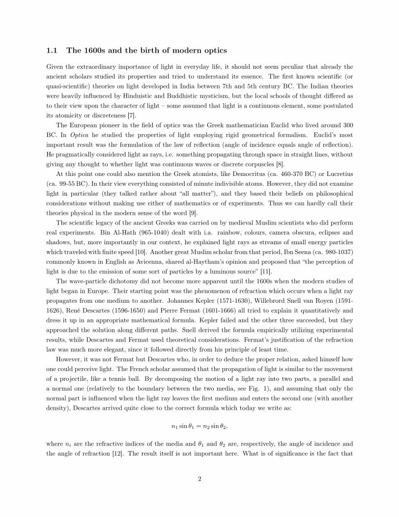
However, it was not Fermat but Descartes who, in order to deduce the proper relation, asked himself how

one could perceive light. The French scholar assumed that the propagation of light is similar to the movement

of a projectile, like a tennis ball. By decomposing the motion of a light ray into two parts, a parallel and

a normal one (relatively to the boundary between the two media, see Fig. 1), and assuming that only the

normal part is influenced when the light ray leaves the first medium and enters the second one (with another

density), Descartes arrived quite close to the correct formula which today we write as:

n1 sin θ1 = n2 sin θ2,

where ni are the refractive indices of the media and θ1 and θ2 are, respectively, the angle of incidence and

the angle of refraction [12]. The result itself is not important here. What is of significance is the fact that

2

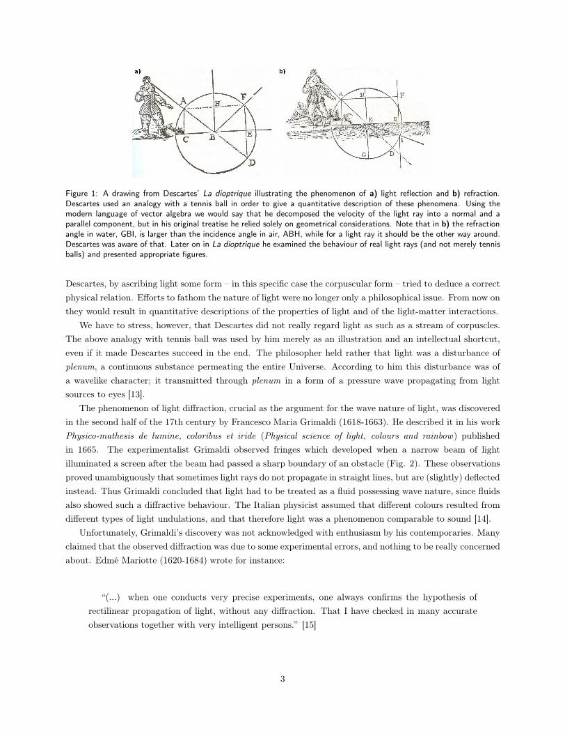
Figure 1: A drawing from Descartes’ La dioptrique illustrating the phenomenon of a) light reflection and b) refraction.Descartes used an analogy with a tennis ball in order to give a quantitative description of these phenomena. Using themodern language of vector algebra we would say that he decomposed the velocity of the light ray into a normal and aparallel component, but in his original treatise he relied solely on geometrical considerations. Note that in b) the refractionangle in water, GBI, is larger than the incidence angle in air, ABH, while for a light ray it should be the other way around.Descartes was aware of that. Later on in La dioptrique he examined the behaviour of real light rays (and not merely tennisballs) and presented appropriate figures.

Descartes, by ascribing light some form – in this specific case the corpuscular form – tried to deduce a correct

physical relation. Efforts to fathom the nature of light were no longer only a philosophical issue. From now on

they would result in quantitative descriptions of the properties of light and of the light-matter interactions.

We have to stress, however, that Descartes did not really regard light as such as a stream of corpuscles.

The above analogy with tennis ball was used by him merely as an illustration and an intellectual shortcut,

even if it made Descartes succeed in the end. The philosopher held rather that light was a disturbance of

plenum, a continuous substance permeating the entire Universe. According to him this disturbance was of

a wavelike character; it transmitted through plenum in a form of a pressure wave propagating from light

sources to eyes [13].

The phenomenon of light diffraction, crucial as the argument for the wave nature of light, was discovered

in the second half of the 17th century by Francesco Maria Grimaldi (1618-1663). He described it in his work

Physico-mathesis de lumine, coloribus et iride (Physical science of light, colours and rainbow) published

in 1665. The experimentalist Grimaldi observed fringes which developed when a narrow beam of light

illuminated a screen after the beam had passed a sharp boundary of an obstacle (Fig. 2). These observations

proved unambiguously that sometimes light rays do not propagate in straight lines, but are (slightly) deflected

instead. Thus Grimaldi concluded that light had to be treated as a fluid possessing wave nature, since fluids

also showed such a diffractive behaviour. The Italian physicist assumed that different colours resulted from

different types of light undulations, and that therefore light was a phenomenon comparable to sound [14].

Unfortunately, Grimaldi’s discovery was not acknowledged with enthusiasm by his contemporaries. Many

claimed that the observed diffraction was due to some experimental errors, and nothing to be really concerned

about. Edmé Mariotte (1620-1684) wrote for instance:

“(...) when one conducts very precise experiments, one always confirms the hypothesis of

rectilinear propagation of light, without any diffraction. That I have checked in many accurate

observations together with very intelligent persons.” [15]

3

Figure 2: Grimaldi’s drawing from Physico-mathesis de lumine, coloribus et iride showing diffraction fringes.

Even though diffraction was not given proper attention in the 1600s, and 150 years had to pass before Thomas

Young conducted his epoch-making interference experiments (see Ch. 1.2), other scientists from that period

did not ignore the possibility that light could have a wave nature. Robert Hooke (1635-1703) and Christiaan

Huygens (1629-1695) can be considered the two main advocates of the wave view in the late 17th century.

Huygens formulated his wave theory of light in Traitbe de la lumiaere (Treatise on light) published in

1690. He proposed that light was emitted from its source as a series of waves propagating in a medium called

“luminiferous ether” which was nothing else than another name for Descartes’ plenum. The particles which

the light source consisted of in this view would move rapidly and would strike the surrounding (and much

smaller) ether particles, which again would agitate another layer of ether particles and so on, so the light

would propagate outwards from the light source in a wavelike fashion. Huygens wrote:

“And I do not believe that this movement can be better explained than by supposing that all

those of the luminous bodies which are liquid, such as flames, and apparently the sun and the

stars, are composed of particles which float in a much more subtle medium which agitates them

with great rapidity, and makes them strike against the particles of the ether which surrounds

them, and which are much smaller than they. (...) Now if one examines what this matter may

be in which the movement coming from the luminous body is propagated, which I call Ethereal

matter, one will see that it is not the same that serves for the propagation of Sound. (...) When

one takes a number of spheres of equal size, made of some very hard substance, and arranges them

in a straight line, so that they touch one another, one finds, on striking with a similar sphere

against the first of these spheres, that the motion passes as in an instant to the last of them. (...)

And it must be known that although the particles of the ether are not ranged thus in straight

lines, as in our row of spheres, but confusedly, so that one of them touches several others, this

does not hinder them from transmitting their movement and from spreading it always forward.”

[16]

Huygens topped his proposition with an important principle, later called after him and also after Augustin-

Jean Fresnel who over one hundred years later supplemented it mathematically (see Ch 1.2). The Huygens-

Fresnel principle says that each point of an advancing wave front can be regarded as a source of a new train

of waves, and that the totality of the advancing wave is in fact a sum of all these secondary wavelets. This

4

view would allow to explain diffraction easily, but in fact Huygens did not pay much attention to interference

phenomena and did not use them as the main argument for the wave nature of light.

It was the corpuscular view that was about to gain upper hand for the whole 18th century. The person

responsible, Isaac Newton (1643-1727), who was commited to several different branches of science and had

great achievements in each of them, summarized his results in optics in his second major book on physical

science, Opticks, published in 1704. However, the treatise New Theory of Light and Colours presented to the

world in 1672 already contained many important and ground-breaking conclusions regarding colours and the

method for extracting them from a sunbeam with the use of a prism.

With this treatise a strife between Newton and another Fellow of the Royal Society, namely Robert Hooke,

began. Newton maintained that light could be explained as a stream of tiny particles propagating in ether

in straight lines from an object to the human eye. Different types of these light particles corresponded to

different primary colours, and by mixing them one could attain other colours as well. Robert Hooke opposed

Newton’s opinion. Hooke was a supporter of the wave hypothesis, which he had employed in order to explain

colours of thin films observed personally under a microscope. Hooke challenged Newton to explain this

phenomenon using the corpuscular hypothesis.

The answer he got was a carefully thought-out compromise where Isaac Newton tried to unite the cor-

puscular and the wave aspects of the light theory. He still maintained that light was a stream of corpuscles,

but he proposed that these corpuscles in a natural way, like stones thrown into water, created ripples in the

ethereal medium permeating all space. The ether undulations could then be responsible for phenomena like

the colours of thin films, claimed Newton; phenomena where the corpuscular view alone was not sufficient.

“The hypothesis of light’s being a body, had I propounded it, has a much greater affinity

with the objector’s own [wave] hypothesis, than he seems to be aware of; the vibrations of the

aether being as useful and necessary in this as in his. For, assuming the rays of light to be small

bodies emitted every way from shining substances, those, when they impinge on any refracting

or reflecting superficies, must as necessarily excite vibrations in the aether, as stones do in water

when thrown into it. And, supposing these vibrations to be of several depths or thicknesses,

accordingly as they are excited by the said corpuscular rays of various sizes and velocities; of

what use they will be for explicating the manner of reflection or refraction; the production of

heat by the sun-beams; the emission of light from burning, putrifying, or other substances, whose

parts are vehemently agitated; the phaenomena of the transparent plates, and bubbles, and of

all natural bodies; the manner of vision, and the difference of colours; as also their harmony and

discord; I shall leave to their consideration, who may think it worth their endeavour to apply this

hypothesis to the solution of phaenomena.” [17]

He pointed out that light could not possibly be only a wave of some kind, because waves have a tendency

towards a spherical propagation, while light rays propagate through space in straight lines which clearly

suggests a corpuscular form. In his reply to Hooke, Newton also stressed that he only wanted to develop a

quantitative theory of colours and their refraction, and that he was not that much concerned about the more

fundamental question of the nature of light [18].

However, during the next few years Newton was drawn into a polemic regarding this very question. A

circle of his critics broadened. Hooke was joined by Huygens, Jesuits Franciscus Linus and Ignace Pardies,

5

and others. The opponents admittedly appreciated Newton’s theoretical and experimental efforts. They

claimed, however, that if one considered different colours to be different types of light particles (and not

different types of undulations), then it would be difficult to explain how this variety of light particles was

created in the first place. Newton replied reluctantly and unconvincingly, because he just did not understand

how someone could not agree with his “self-evident” theory [14].

Isaac Newton elaborated on his corpuscular view in Hypothesis of light presented to the secretary of the

Royal Society in December 1675. There he again put forward the conciliatory hypothesis where both the

corpuscular and the wave assumption were utilized. Light sources emit light particles, and the light particles

make ether vibrate. He stressed that light is neither ether nor its undulatory motion, but something else that

propagates from the luminous bodies [19].

The discussion about the nature of light reached a stalemate. The publication of Huygens’ Traitbe de la

lumiaere in 1690 did not make Newton change his mind. Admittedly they both agreed that ether is necessary

for the propagation of light. However, Huygens’ believed that light is the movement (or oscillations) of the

ether particles, while Newton maintained that light corresponds to some other type of particles which only

travel through ether (possibly interacting with the ether substance as well).

Robert Hooke died in 1703. In November the same year Newton was elected a new president of the Royal

Society (after the former president, Lord Somers, had died). Newton ruled the English science with an iron

hand till his death in 1727, and used the distinguished position to ruthlessly fight his scientific opponents.

No one dared to contradict his corpuscular view on the nature of light any longer, and Newton himself made

this view very clear in his canonical work Opticks where in the very first definition he stated that

“Defin. I. By the Rays of Light I understand its least Parts, and those as well Successive in

the same Lines, as Contemporary in several Lines. For it is manifest that Light consists of Parts,

both Successive and Contemporary; because in the same place you may stop that which comes

one moment, and let pass that which comes presently after; and in the same time you may stop

it in any one place, and let it pass in any other. For that part of Light which is stopp’d cannot

be the same with that which is let pass. The least Light or part of Light, which may be stopp’d

alone without the rest of the Light, or propagated alone, or do or suffer any thing alone, which

the rest of the Light doth not or suffers not, I call a Ray of Light.” [20]

Thus the corpuscular view dominated the scientific stage for around 100 years. The research progress in optics

in the 18th century was small. Instead, analytical mechanics, thermodynamics, electricity and magnetism

were being developed. The theory of Huygens was forgotten and even Leonhard Euler (1707-1783), who

argued in Nova theoria lucis et colorum (1746) that diffraction could be explained more easily by the wave

hypothesis, did not refer to it. One had to wait 50 more years before another prominent English scientist set

out to change the optical paradigm. But even after the wave view had finally triumphed over the corpuscular

view in the 19th century, Newton’s ideas about the nature of light were still treated with a great deal of

respect.

“So great, however, was Newton’s fame among men of science that a number of writers on

optics, especially among the British, took care to inform their readers that Newton’s corpuscular

6

theory, while clearly incorrect, was nevertheless a very ingenious creation and had been fully able

to explain all of the facts about light known in Newton’s day. In other words, this theory was

not wholly relegated to the realms of the antique and the curious but was rather presented to the

reader with an apology and a discussion of the 17th-century situation in physics.” [21]

1.2 1800s and the triumph of the wave theory of light

The polymath Thomas Young (1773-1829), later called “the last man who knew everything”, contributed

to the scientific understanding of physics, physiology and Egyptology. When he was still a student, he

presented a treatise on the structure and accommodation of the eye, becoming the founder of physiological

optics. Then he got interested in the nature of light, and after a series of experiments he tried to revive the

almost forgotten wave theory of light.

In two lectures given to the Royal Society in 1800 and 1801 Young carefully reminded his colleagues of the

possibility that light might be perceived as a wave propagating in ether. He was well aware of the dominant

position of the corpuscular view supported by the late Newton’s enormous authority. Therefore he reminded

his listeners that Newton himself had not completely rejected the wave view, and then advanced following

postulates:

“1. That a luminiferous ether, rare and elastic in a high degree, pervades the whole universe.

2. That undulations are excited in this ether whenever a body becomes luminous. And,

3. That the sensation of different colours depends on the frequency of vibrations excited by

light in the retina.” [22]

Young presented a number of propositions describing these ether undulations qualitatively. In the last of

them he claimed that

“[w]hen two undulations from different origins coincide either perfectly or very nearly, in

direction, their joint effect is a combination of the motions belonging to each. (...) This last

Proposition may be considered as the general result of the whole investigation.” [22]

Thomas Young elaborated on the interference phenomena in his later treatises. He never based his reasoning

on pure theoretical assumptions, but performed actual interference experiments, both with water and light,

in order to emphasize the wave analogy. Thus very soon he could find a hard experimental proof for light

diffraction, and presented it to the Royal Society in November 1803.

“In making some experiments on the fringes of colours accompanying shadows, I have found

so simple and so demonstrative a proof of the general law of the interference of two portions of

7

light, which I have already endeavoured to establish (...) Exper. 1: I made a small hole in a

window-shutter, and covered it with a piece of thick paper, which I perforated with a fine needle.

For greater convenience of observation, I placed a small looking glass without the window-shutter,

in such a position as to reflect the sun’s light, in a direction nearly horizontal, upon the opposite

wall, and to cause the cone of diverging light to pass over a table, on which were several little

screens of card-paper. I brought into the sunbeam a slip of card, about one-thirtieth of an inch in

breadth, and observed its shadow either on the wall, or on other cards held at different distances.

Besides the fringes of colours on each side of the shadow, the shadow itself was divided by similar

parallel fringes, of smaller dimensions, differing in number, according to the distance at which

the shadow was observed, but leaving the middle of the shadow always white. Now these fringes

were the joint effect of the portions of light passing on each side of the slip of card and inflected,

or rather diffracted, into the shadow.” [23]

Young conducted several other experiments and gathered a solid amount of evidence that light interfered.

Thus his results strongly suggested that light had a wave nature. Unfortunately, many other scientists

mercilessly criticized Young’s methods and conclusions. The authority of Newton was still strong, and

his corpuscular view was too respected to allow one juvenile scientist to establish a completely new theory,

especially when this theory was qualitative rather than mathematical. Young got discouraged and abandoned

his optical research for some years.

On the other side of the English Channel, however, progress in optics was still being made by French

physicists. Étienne-Louis Malus (1775-1812) discovered polarization of light by reflection in 1809 and ex-

plained double refraction of light in crystals in 1810. Pierre-Simon Laplace (1749-1827) and Jean-Baptiste

Biot (1774-1862) worked out a mathematical theory describing propagation of light in crystals. Unfortu-

nately, all these scientists still employed the corpuscular view, and in order to explain the phenomenon of

polarization Malus assumed that the light corpuscles are not rotationally symmetrical, but somewhat elon-

gated. The angle between the direction of their propagation and their, say, major axes, were supposed to

correspond to a given polarization.

It was another French scientist, Augustin Fresnel (1788-1827), who not only approved of Young’s wave

theory, but got inspired by it and extended it considerably. Fresnel synthesized the wave ideas of Young as

well as Christiaan Huygens’ using a rigid mathematical apparatus, and showed how one could apply them in

order to explain quantitatively a large class of optical phenomena. The predictive powers of Fresnel’s work

were in fact so great that they gave rise to one of the best known anecdotes in the annals of the history of

science.

Fresnel submitted his work to a competition held by Académie des Sciences in 1819 where the best theory

on diffraction was to be awarded. At first the work was met with scepticism by the prominent members of the

commitee – Dominique Arago, Siméon Poisson, Laplace and Biot among the others – because Fresnel’s model

discarded the corpuscular view. Poisson, though, liked mathematics very much (even though he disagreed

with the physical interpretation) and pushed the original calculations of the author even further. In the

end he predicted that, according to Fresnel’s theory, the shadow of a circular disc was supposed to have a

small bright spot in its centre. No one had observed such a thing before, so it seemed that the model was

erroneous. Arago proposed to put it to a decisive experimental test. The commitee expected that no bright

spot would appear, and that the model could then be rejected on the grounds of its absence. Surprisingly,

8

Arago ended up with discovering the spot (from now on called Arago spot), so the accuracy of Fresnel’s

model was established and he could receive the main prize in the competition [24].

In the meantime Young and Fresnel corresponded with each other, and, of course, the English scientist

approved very much of the results of his French colleague. It seemed that the wave theory of optics could

overturn the corpuscular view after all. Paradoxically, the polarization of light presented the largest problem,

because in the beginning Young and Fresnel had assumed that the ether undulations were longitudinal, in

analogy with sound waves, so the polarizational degree of freedom was missing. However, soon an intellectual

step forward was made and Thomas Young proposed in 1817 to provide the undulations with a transverse

component. Four years later Fresnel proved that polarization could be explained only if there was no longi-

tudinal component at all, just the transverse one. It took some time before other physicists fully accepted

this revelation [14].

Thanks to the mathematical framework developed by Fresnel, the wave theory of light gained a broad

acceptance in the following years. New developments helped to establish it further. For instance, Christian

Doppler (1805-1853) utilized it to explain the effect (later called by his name) that caused shifts in the stellar

frequency spectra (though probably the same effect could be explained using the corpuscular view). However,

Doppler’s result had to pale into insignificance in comparison with a great breakthrough that was soon about

to happen: the discovery that not only electricity and magnetism are intimately connected, but also that the

realm of optics lies de facto inside the realm of electromagnetism.

We are not going to present even a short summary of the history of electromagnetism since such a

digression would not have anything to do with the development of the notion of wave-particle duality. Thus,

let us rudely ignore the achievements of Gilbert, Coulomb, Volta, Oersted, Ampère, Faraday and many

others, and proceed directly to Maxwell’s synthesis of the electromagnetic laws and its repercussions for the

understanding of the nature of light.

James Clerk Maxwell (1831-1879) created the classical theory of electromagnetism by incorporating the

results of several other physicists into a coherent mathematical framework. In order to achieve this consistency

he had to somewhat change the nomenclature used by his colleagues, and fill all gaps with a thorough

qualitative discussion of the electromagnetic phenomena. Possibly the most important conclusion of the

electromagnetic theory was that the electromagnetic phenomena propagated in an undulatory fashion through

ether. Thus Maxwell could predict, on purely theoretical grounds, the existence of electromagnetic waves1.

A Treatise on Electricity and Magnetism published by him in 1873 became a physical milestone – but it

did not happen immediately, because for some time the rival electrodynamic theory of Wilhelm Weber was

dominant, especially in Germany.

Maxwell understood that the electromagnetic theory could be used to explain the phenomenon of light;

moreover, he pondered if light could not in fact be some kind of electromagnetic propagation. Let us quote

an important fragment of the treatise:

“781. In several parts of this treatise an attempt has been made to explain electromagnetic

phenomena by means of mechanical action transmitted from one body to another by means of

a medium occupying the space between them. The undulatory theory of light also assumes the

1One should be reminded that Maxwell did not write down the equations called after him the way they are known to physiciststoday. The Scotch scientist was using the quarterion notation instead of the vectorial one. It was Oliver Heaviside (1850-1925)who put the equations in their modern form.

9

existence of a medium. We have now to shew that the properties of the electromagnetic medium

are identical with those of the luminiferous medium.

To fill all space with a new medium whenever any new phenomenon is to be explained is by

no means philosophical, but if the study of two different branches of science has independently

suggested the idea of a medium, and if the properties which must be attributed to the medium in

order to account for electromagnetic phenomena are of the same kind as those which we attribute

to the luminiferous medium in order to account for the phenomena of light, the evidence for the

physical existence of the medium will be considerably strengthened.

But the properties of bodies are capable of quantitative measurement. We therefore obtain the

numerical value of some property of the medium, such as the velocity with which a disturbance

is propagated through it, which can be calculated from electromagnetic experiments, and also

observed directly in the case of light. If it should be found that the velocity of propagation of

electromagnetic disturbances is the same as the velocity, and this not only in air, but in other

transparent media, we shall have strong reasons for believing that light is an electromagnetic

phenomenon, and the combination of the optical with the electrical evidence will produce a

conviction of the reality of the medium similar to that which we obtain, in the case of other kinds

of matter, from the combined evidence of the senses.” [25]

To recapitulate: From the two assertions, that the electromagnetic phenomena propagate through ether as

waves, and that light also propagates through ether as waves, Maxwell reached a rather obvious conclusion

that light is an electromagnetic phenomenon. But this reasoning was not only qualitative. On the contrary:

Maxwell noticed a remarkable correspondence between some electromagnetic quantities and the speed of

light. Using today’s physical symbols, we would say that he discovered that

√ǫµ ≈ c−1

where ǫ is the electric permittivity, µ is the magnetic permeability and c is the speed of light. However,

Maxwell expressed his conclusions quite carefully:

“It is manifest that the velocity of light and the ratio of the units are quantities of the same

order of magnitude. Neither of them can be said to be determined as yet with such a degree of

accuracy as to enable us to assert that the one is greater or less than the other. It is to be hoped

that, by further experiment, the relation between the magnitudes of the two quantities may be

more accurately determined.” [25]

The scientific community did not have to wait long for an experimental confirmation of the electromagnetic

waves postulated by Maxwell. Heinrich Hertz (1857-1894) demonstrated propagation of these waves in air in

the second half of the 1880s. In Hertz’s experiment one observed how electromagnetic undulations, excited

in the primary conductor using Ruhmkorff coil, were wirelessly transmitted to a secondary conductor placed

several meters away. Thereafter Hertz showed how these waves reflected from walls of a room (effectively

creating standing waves). In a similar fashion one could examine their refraction and interference.

10

It seemed that the wave theory of light achieved its ultimate victory. In less than 100 years, thanks

to the efforts of physicists like Young, Fresnel, Maxwell and Hertz, the corpuscular theory of Newton had

been knocked down from the pedestal. Admittedly the falsification was indirect, since instead of finding

erroneous conclusions of the corpuscular view, the scientists had rather showed how the wave view could

be used to explain many natural phenomena in a strictly mathematical way. The wave theory of light

seemed completely consistent as well, and the conclusion was very elegant: Visible light is only one type of

electromagnetic undulations which propagates transversely and with different oscillation frequencies through

ether.

Two problems remained. Albert Abraham Michelson (1852-1931) and Edward Morley (1838-1923), using

a special kind of interferometer, tried to measure the speed of Earth relatively to ether – and failed completely.

Their results led to the astounding conclusion that ether, which scientists had taken for granted at least since

1600s, in fact did not exist. This discovery had colossal implications for classical mechanics, and inspired

Albert Einstein to propose his special theory of relativity in 1905. But for optics it did not really mean

that much. After all, one could just move on to the assumption that the electromagnetic waves propagate

in vacuum, and although such a statement was difficult to accept from the then-valid philosophical point of

view, it did not matter for the quantitative part of the theory.

The second problem was much more grave: The electromagnetic theory was not able to fully explain

either the black-body radiation or the photoelectric effect. However, no one suspected that a new paradigm

would be needed in order to resolve these discrepancies. On the contrary – the common belief in that time

was that theoretical physics was completed. “The grand underlying principles have been firmly established

(...) further truths of physics are to be looked for in the sixth place of decimals”, claimed Michelson in 1894

[26].

Only six years after this proud statement, the quantum mechanics was born. Our picture of light soon

had to be reshaped once again.

1.3 The early 1900s and the rise of quantum mechanics

The recovery of the corpuscular view is directly connected to the origin of quantum mechanics, with Max

Planck (1858-1947) traditionally considered to be its father. In 1890s Planck investigated the theoretical

frontier between the well-established classical mechanics and the relatively new sciences of electrodynamics

and termodynamics. Specifically, he wanted to show how the second law of thermodynamics could be de-

rived from some fundamental model for heat oscillators, a model firmly rooted in the principles of classical

mechanics and electrodynamics. However, his scheme met huge difficulties, largely because Planck opposed

atomistic view and did not want to accept the statistical interpretation of the second law given by Ludvig

Boltzmann (1844-1906). His attitude to Boltzmann’s theory gradually changed to become more positive, and

in the last years of the decade Planck started to work on another, related issue – the spectral distribution of

the black-body radiation.

The black-body spectral density (the radiation energy density per unit frequency) had been described by

an empirical law proposed by Wilhelm Wien (1864-1928) in 1886. Planck set out to find a rigorous theoretical

derivation of Wien’s law. In the meantime, very precise measurements on the black-body radiation, conducted

11

in 1899 in Berlin by Otto Lummer and Ernst Pringsheim [27], showed that Wien’s formula was not completely

valid, because it broke down at low frequencies. Planck was not only able to improve the formula, but also,

using his superior insights gained previously from the study of the second law of thermodynamics, to show

how the formula followed from the first principles. However, in order to succeed, Planck had to introduce two

novel ideas. He postulated a new constant of nature, h (later called by his name); and he claimed that the

energy involved in the radiation process was divided into minute, but finite portions. Max Planck annouced

his final results2 to the scientific community in a famous lecture given in Berlin on December 14, 1900. His

formula, later called Planck’s law (see Ch. 3.1), was in perfect accordance with the experimental results, and

the derivation seemed elegant and faultless [28].

The date of Planck’s lecture is today commonly recognized as the day the quantum mechanics was

born. However, it should be stressed that Planck himself considered the quantization of energy merely as a

mathematical trick, “a purely formal assumption” [29]. Most of his colleagues apparently shared this view;

in any case, they were not aware that a revolution in physics was just happening. Although Planck probably

understood that a possible physical interpretation of this “mathematical trick” was discrete absorption and

emission of light by matter, he believed the whole quantization scheme to be only a temporary feature of the

model, something to be removed by further improvements. But the foundations for the quantum mechanics

had already been laid, and the first big step towards the “new” corpuscular view of light had been made.

It was Albert Einstein (1879-1955) who first really appreciated the idea of Planck and extended it in order

to explain the photoelectric effect. The photoelectric effect was discovered by Hertz in 1887 and clarified

by Philipp von Lenard in 1902. The effect is a phenomenon where electrons are emitted from a material

illuminated by electromagnetic radiation with high enough frequency (see Ch. 3.3). From Maxwell’s theory

one would expect that the radiation intensity alone should decide if the electrons got emitted, but the

experimental reality showed that the radiation frequency was an even more important factor [30].

Einstein presented an innovative solution to the problem in 1905, but his convictions about the nature

of light related to the photoelectric effect mattered more than the formulas reproducing the experimental

results.

“In fact, it seems to me that the observations on “black-body radiation”, photoluminescence,

the production of cathode rays by ultraviolet light and other phenomena involving the emission

or conversion of light can be better understood on the assumption that the energy of light is

distributed discontinuously in space. According to the assumption considered here, when a light

ray starting from a point is propagated, the energy is not continuously distributed over an ever

increasing volume, but it consists of a finite number of energy quanta, localised in space, which

move without being divided and which can be absorbed or emitted only as a whole.” [31]

Thus Einstein went much further in his argumentation than Planck. He assumed that not only the absorption

2 Many popular accounts claim erroneously that Planck aimed to resolve the so-called “ultraviolet catastrophe”, i.e. the

paradox where classical physics predicted an infinite amount of energy emitted by a black body at high frequencies. This is

emphatically not true, because the “catastrophe” was first expressed through the Rayleigh-Jeans formula proposed as late as in

1905; and the term “ultraviolet catastrophe” was coined by Paul Ehrenfest only in 1911. In other words, the paradox did never

really had time to become a problem, because Planck’s law had solved it before it was explicitly formulated [28].

12

and emission of radiation occurs in a discrete fashion, but also that the propagation of light in space is of

a quantum character. Most other physicists were against such a radical hypothesis, not only because of its

far-reaching consequences and (at least partial) negation of the wave view, but also because the explanation

of the photoelectric effect turned out in the end to be possible by means of the classical electromagnetic

theory. This had been achieved by several persons: J. J. Thomson in 1910, Arnold Sommerfeld and Peter

Debye in 1911, and, most notably, by Owen Richardson in 1912 (see Ch. 3.3) [32].

During the next years Albert Einstein has become a highly respected scientist, largely due to his special

and general theory of relativity. However, many scientists still did not regard the corpuscular idea seriously,

because the wave view, being firmly grounded in Maxwell’s theory, was so much appealing as an explanation

of the physical reality of light. As always, in order to convince the skeptics, one needed an unambiguous

experiment. Such an experiment was conducted in 1922 by Arthur Compton (1892-1962) who examined

X-ray scattering. Compton noticed that the problematic experimental results could be easily explained if one

adapted the corpuscular view of the radiation. It was, however, not easy for him to embrace this idea, and

he employed it only as the last resort. First he had tried to explain his data by assuming large size of the

electron (i.e. larger than the measurements of Ernest Rutherford had indicated) and by aid of the Doppler

effect. In the end Compton had to admit that the corpuscular hypothesis offered the easiest explanation,

because it implied that the radiation and the electrons exchanged momentum like minute particles, just like

Compton’s experiments had suggested (see Ch 3.4).

Einstein’s corpuscular considerations backed up by Compton’s results propelled anew the interest in the

nature of light. On the one hand, the corpuscularity of light seemed at least partly confirmed; on the other

hand, the “old” interference phenomena were still taking place, and in order to explain them the wave view

seemed to be necessary. Physicists started to look for a way to avoid the apparent paradox. Fortunately, the

intellectual atmosphere of that period encouraged new and bold ideas – after all Niels Bohr (1885-1962) had

just proposed a new atomic model, and many scientists had understood that another revolution in physics,

based on quantum mechanical ideas, was imminent.

John Slater (1900-1976) advanced the notion of “virtual oscillators” which could be used to unite the

classical theory of electromagnetic field with the quantum theory of light. Bohr, Slater and Hendrik Kramers

extended this notion and created a new theory of radiation, so-called BKS theory [34]. However, it had one

large disadvantage: It implied that the energy and momentum exchange in microscopical physical processes

were of a statistical nature, so the energy and momentum conservation principle were no longer valid. Such

a suggestion sounded like a heresy to the scientific community, and was soon experimentally refuted [35].

It was Louis de Broglie (1892-1987) who in his doctoral thesis in 1924 put forward the extraordinary idea

which in some sense solved the problem of the dualistic nature of light by extending it to the rest of the

world, i.e. to all matter. De Broglie assumed that, just as light sometimes showed corpuscular and sometimes

undulatory behaviour, the atomic matter possessed in addition a wave nature (see Appendix C) [36]. Even

though the idea might have sounded like a bad joke in the beginning, the laboratory proofs confirming de

Broglie’s hypothesis had already existed, but the connection had not been noticed immediately. In 1921

Clinton Davisson and Charles Kunsman published the results of their experiments in which electron beams

were undergoing dispersion and reflection from crystals. The angular distribution of the reflected electrons

suggested in fact a possibility of their wave nature. The controversial proposal of de Broglie encouraged the

scientific community to examine the matter more closely, and in 1927 the hypothesis had been ultimately

confirmed. Davisson and Lester Germer, by firing electrons at a crystalline nickel target obtained a diffractive

13

pattern which matched exactly the theoretical predictions of de Broglie [37]. Three years later, in 1930, Otto

Stern and Immanuel Estermann observed a similar diffraction of much larger helium atoms and hydrogen

molecules [38].

The wave-particle duality problem fully emerged. No one could deny that in the macroscopic world

matter has entirely corpuscular properties, but in the same breath no one could ignore the results of the

Davisson-Germer experiment neither; the experiment which had clearly demonstrated that on microscopic

level the matter – or at least its smallest constituents – showed an undulatory behaviour and was able to

interfere. One was thus unwillingly forced to admit that the matter, in a difficult to perceive sense, is both

particles and waves. This effectively eliminated the old wave-or-particle dillemma with regard to light: Since

the physical situation in the realm of light was completely analogous, i.e. some experiments and models

emphasized the corpuscular nature of light and other experiments and models the undulatory nature, one

could apply a similar conclusion here and claim that light is both particle and wave at the same time.

Niels Bohr tried to explain the highly philosophical problem of the wave-particle duality using so-called

complementarity. A whole school of thought has been built around this concept, and we relegate the discussion

of the principle to Chapter 9.2. Here suffice it to say that complementarity, instead of answering the central

question “Are matter and light particles or waves?”, effectively claimed that this question is meaningless

and presented an exhaustive justification for such a claim. On the quantitative side complementarity was

supported by the uncertainty principle advanced by Werner Heisenberg (1901-1976) in 1927 which implied

that it was fundamentally impossible to simultaneously measure the position and the momentum of a physical

object with an arbitrary high precision (see Appendix A).

After the discovery of the uncertainty principle, neither new experimental breakthroughs nor fully suc-

cessful theoretical models have considerably changed the shape of the wave-particle duality problem. Several

new physical ideas were proposed in order to resolve it, but they did not gain broad acceptance since they had

not been supported strongly enough by empirical data. Arguably the most noteworthy among them was the

Bohmian interpretation of quantum mechanics developed by David Bohm (1917-1992) in the early 1950s [39].

Bohm built on the ideas of Louis de Broglie and postulated that every material particle is accompanied by a

field which guides the motion of the particle. This field (called the pilot wave by de Broglie and the quantum

field by Bohm) evolves according to the Schrödinger equation of quantum mechanics and is responsible for

the undulatory behaviour of matter (see Ch. 9.3).

Another interesting (but tentative) theory related to the wave-particle duality problem was put forward

by Edwin Jaynes (1922-1998), a proposer of the neoclassical model of radiation [40]. Jaynes aimed to modify

quantum electrodynamics by eliminating its inherent need for quantization of electromagnetic field. Thus

Jaynes wanted to create a physical model as successful as quantum electrodynamics, but where only the

interactions between light and matter were quantized, not light itself. Discrepancies with experimental

results eventually extinguished the interest of the physical community for the neoclassical model.

Quantum mechanics has not managed to radically change our way of perceiving the wave-particle duality

after the 1930s, but the problem kept on receiving attention in the second half of the last century. It was

largely due to three discoveries that took place around 1960 and completely refreshed the science of optics.

In 1955 Robert Hanbury Brown and Richard Twiss constructed a new type of stellar interferometer which

did not measure the correlations of the electric and magnetic field strenghts, but the correlations between

intensities [41]. Such a new angle of approach immediately raised several new and interesting questions about

light interference. The effects discovered by Hanbury Brown and Twiss were soon explained by themselves

14

as correlations of the fluctuations in the electromagnetic field. However, it was demonstrated by others that

such effects could be also directly related to the corpuscular view of light, and understood as bunching of

photons (i.e. phenomenon where photons occur in bunches) [42].

The interferometry experiment due to Hanbury Brown-Twiss is often considered to be the experimental

confirmation of classical theory of optical correlations (see Ch. 4). Roy Glauber showed in 1963 [43] how

one can translate the notion of optical coherence to quantum terms [43] and obtain new predictions not

accounted for by the classical theory (see Ch. 4.4). These predictions were later confirmed by experiments

with nonclassical states of light (see Sect. 5.1.4).

Between Hanbury Brown-Twiss’ experiment and Glauber’s paper, Theodore Maiman demonstrated in

1960 the first working laser [6]. While industry embraced the new invention and used it to produce several

devices that changed our everyday world (CD players being arguably the most prominent example), scientists

could use the laser as a new tool for exploring the corpuscular and undulatory properties of light. Thanks to

the efforts of Hanbury Brown, Twiss, Maiman, Glauber and others, a new branch of physics – quantum optics

– became firmly established in the early 1960s, and other scientists could start following a new scientific path.

The aforementioned events stimulated the interest in the general properties of light, but several experi-

ments conducted quite recently touched directly upon the problem of the wave-particle duality. In 1989 the

team of Akira Tonomura conducted for the first time the famous double-slit experiment with electrons in

carefully controlled laboratory conditions (see Appendix C) [5]. In 1999 Anton Zeilinger and his colleagues

performed another experiment of the same kind, but with fullerene molecules instead of electrons [44]. The

interference pattern was again obtained, confirming that also particles much larger than electrons are able

to behave in accordance with de Broglie relations.

The somewhat controversial Afshar experiment was one of the most recent words uttered on the matter

of the wave-particle duality of light [45]. It was first conceived and carried out by Shahriar Afshar in 2005

(but later repeated in an improved form). The experiment is assumed by some to demonstrate a paradox

of the wave-particle duality, because it seemingly allows to observe both the corpuscular and the undulatory

behaviour of light at once [46]. However, a consensus has not been yet reached. The Afshar experiment and

its possible implications will be analyzed in Chapter 8.

Thus we have followed, in a rather abridged way, the historical development of the wave-particle duality

notion. We have seen how it evolved from an either-or question concerning solely light to a much deeper

problem regarding the dual nature of the totality of radiation and matter. Although today the paradox is

phrased in the same way as it was in the 1930s, in the meantime the progress of science, especially in the

framework of quantum optics, has highlighted some novel features of the duality (as, for instance, photon

bunching and antibunching).

The author would like to make one final remark. The wave-particle duality is a beautiful illustration

of applied Hegelian dialectic. This philosophical doctrine formulated by Heinrich Chalybäus (and not by

Georg Hegel, as the name suggests) states that in the development of new ideas we can (usually) distinguish

three phases: the initial thesis, the contradictory antithesis and the final synthesis which resolves the tension

between the first two and offers a compromise solution. As we have seen in the above chapter, the wave

theory of light was used to negate the corpuscular statements of Isaac Newton, and then quantum mechanics

united both views through the wave-particle duality paradox. But in the Hegelian dialectic the synthesis is

by no means the final word in the whole story, because usually it gives rise to a new thesis and the scheme

15

repeats itself. It remains to be seen if the wave-particle duality of de Broglie and Bohr will be challenged by

another explanation of the quantum-mechanical phenomena, and if the discussion about the nature of light

and matter will be reincarnated in some other form.

16

2 The classical and the quantum descriptions of light

After having discussed the historical development of the wave-particle duality notion, we are now ready to

consider the strictly physical aspects of the problem. In the following chapters we will review, compare and

comment chosen elements of the classical and quantum-mechanical theories regarding either the undulatory

or the corpuscular nature of radiation.

We start by giving a short presentation of Maxwell’s electromagnetic theory embedded into Maxwell’s

equations which unanimously declare light to be an electromagnetic wave (Ch 2.1). Another approach to

radiation based on quantum harmonic oscillator (Ch. 2.2) and quantization of electromagnetic modes (Sects.

2.3.1-2.3.2) is possible as well. In this way we introduce the photon number states (Sects. 2.3.3-2.3.4) and

suppress the wave aspect of radiation. Furthermore, one can also employ the coherent state formalism which

represents “classical” states of light (Ch. 2.4).

Before we proceed, we have to stress that what follows is in fact a strongly abridged review of the basic

elements of the essential theories. Although we try to keep the consistency level high, move from one stage to

another in a smooth fashion (that is, highlighting the links between the stages) and delve into the relevance

the different theories have for the wave view or for the corpuscular view, it is by no means possible to deal

with the chosen theories exhaustively. For instance, dedicating only three pages to a section called “Maxwell’s

electromagnetic theory” may seem as an insult to the theory; or, while exploring the possibility for quantizing

the electromagnetic modes, we delibaretely ignore the fact that the huge domain of quantum field theory is

right behind the corner.

2.1 Maxwell’s electromagnetical theory

The electromagnetic field is described classically by two vectorial quantities: the electric field E and the

magnetic field B. Generally these vector fields are not constant, but position- and time-dependent, so we

should rather write E = E(r, t), B = B(r, t). More importantly, they also depend on each other, and the

17

way they are linked together in the physical space is quantified by Maxwell’s equations3:

∇× B = µJ + µǫ∂E

∂t(1)

∇× E = −∂B∂t

(2)

∇ ·B = 0 (3)

∇ ·E =ρ

ǫ(4)

The meaning of the symbols should be evident, but for the sake of completeness let us quickly define them.

J and ρ are, respectively, total current density and total charge density (total meaning both free and bound

currents / charges are to be considered); ǫ is the electric permittivity which describes how the electric field

affects and is affected by the actual medium; and µ is the magnetic permeability which describes how the

magnetic field affects and is affected by the actual medium. In vacuum the values of the permittivity and

the permeability are written ǫ0 and µ0, respectively, with the values 4:

ǫ0 ≡ 8.85 × 10−12 F/m

µ0 ≡ 4π × 10−7 H/m.

Thus in free space Maxwell’s equations reduce to:

∇× B = µ0ǫ0∂E

∂t(5)

∇× E = −∂B∂t

(6)

∇ ·B = 0 (7)

∇ ·E = 0 (8)

Maxwell’s equations have to be supplemented by the Lorentz force law governing the motion of a point

charge in an electromagnetic field:

F = q(E + [v × B]). (9)

Here F is the force working on the particle, q is the charge of the particle and v is its velocity.

A great variety of electrostatic and electrodynamic phenomena can be quantitatively described using

these five simple equations. Undoubtedly their most important prediction is that of the electromagnetic

waves which paves the way to the realm of electrodynamics. More precisely, from Maxwell’s equations one

can deduce the wave equation which suggests existence of some kind of electromagnetic waves. To derive the

wave equation in free space we will need one of the vector identities:

∇× (∇× Z) = ∇(∇ · Z) −∇2Z

3We present Maxwell’s equation in the differential form, but they can equivalently be written in the integral form. See, forinstance, Rao [47].

4The modern convention is to define both ǫ0 and µ0 in such a way that ǫ0µ0 = c−2 where c is the speed of light. However,it does not mean that Eq. (12) (see below) should be considered trivial. Historically speaking, both the permittivity andthe permeability were initially measured, and the scientists did not know about their connection with c. It was Maxwell whodiscovered the relation given by Eq. (12), and only afterwards it was used to motivate the definition.

18

which is valid for any vector field Z. Now, let us apply the curl operator to Eq. (6), make use of the vector

identity above and then simplify the resulting expression using Eq. (5) and Eq. (8):

∇× (∇× E) = ∇×(

−∂B∂t

)

∇(∇ · E) −∇2E = −∂(∇× B)

∂t

−∇2E = −µ0ǫ0∂2E

∂t2

∇2E − µ0ǫ0∂2E

∂t2= 0. (10)

An identical equation can be derived for B. Thus all components of the electric and the magnetic field satisfy

the wave equation which, for some scalar quantity u, can be written as

∇2u− 1

v2

∂2u

∂t2= 0 (11)

where v is the phase velocity of the wave. Physically speaking we are now considering a highly idealised

situation where the wave under examination propagates far away from both the source and any materials

that could influence the fields. However, our simplification should not be regarded as nonaccurate, because

in any realistic situation the undulatory aspect will be present and as strongly pronounced as it is now.

The only difference would be a complication of the differential equations involved due to (possibly complex)

boundary conditions.

Since the electromagnetic radiation is known to propagate in vacuum with the speed of light c, we see

that the value of the speed of light emerges from the classical electromagnetic theory and can be calculated

using the electric permittivity and the magnetic permeability. From Eq. (10) it follows that

c =1√ǫ0µ0

, (12)

a relation discovered by Maxwell himself and already commented upon in Chapter 1.2 of the thesis.

The general solution of the electromagnetic wave equations in free space (far away from the source and

materials) may be given in the complex form:

E(r, t) = E0e−j(k·r−ωt) (13)

B(r, t) = B0e−j(k·r−ωt). (14)

k represents the wave vector, i.e. the propagation direction of the wave, and ω is the angular frequency of the

wave, related to the oscillation frequency f as ω = 2πf . The physically measurable electromagnetic waves

are obtained by taking the real parts of the expressions above.

If we now insert Eq. (13) and Eq. (14) into Eq. (5) and Eq. (6), we will eventually find that

k × B0 = −ωǫ0µ0E0

k × E0 = ωB0.

It follows that the electric field is perpendicular to both the wave vector and the magnetic field, while the

19

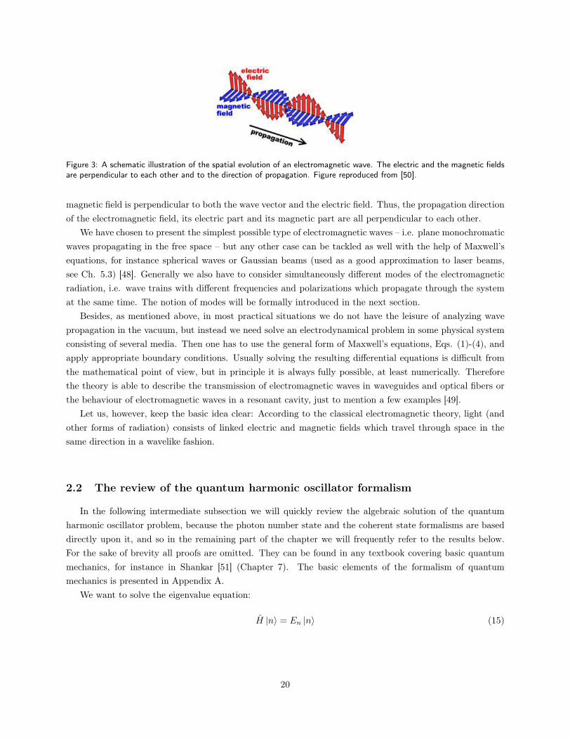
Figure 3: A schematic illustration of the spatial evolution of an electromagnetic wave. The electric and the magnetic fieldsare perpendicular to each other and to the direction of propagation. Figure reproduced from [50].

magnetic field is perpendicular to both the wave vector and the electric field. Thus, the propagation direction

of the electromagnetic field, its electric part and its magnetic part are all perpendicular to each other.

We have chosen to present the simplest possible type of electromagnetic waves – i.e. plane monochromatic

waves propagating in the free space – but any other case can be tackled as well with the help of Maxwell’s

equations, for instance spherical waves or Gaussian beams (used as a good approximation to laser beams,

see Ch. 5.3) [48]. Generally we also have to consider simultaneously different modes of the electromagnetic

radiation, i.e. wave trains with different frequencies and polarizations which propagate through the system

at the same time. The notion of modes will be formally introduced in the next section.

Besides, as mentioned above, in most practical situations we do not have the leisure of analyzing wave

propagation in the vacuum, but instead we need solve an electrodynamical problem in some physical system

consisting of several media. Then one has to use the general form of Maxwell’s equations, Eqs. (1)-(4), and

apply appropriate boundary conditions. Usually solving the resulting differential equations is difficult from

the mathematical point of view, but in principle it is always fully possible, at least numerically. Therefore

the theory is able to describe the transmission of electromagnetic waves in waveguides and optical fibers or

the behaviour of electromagnetic waves in a resonant cavity, just to mention a few examples [49].

Let us, however, keep the basic idea clear: According to the classical electromagnetic theory, light (and

other forms of radiation) consists of linked electric and magnetic fields which travel through space in the

same direction in a wavelike fashion.

2.2 The review of the quantum harmonic oscillator formalism

In the following intermediate subsection we will quickly review the algebraic solution of the quantum

harmonic oscillator problem, because the photon number state and the coherent state formalisms are based

directly upon it, and so in the remaining part of the chapter we will frequently refer to the results below.

For the sake of brevity all proofs are omitted. They can be found in any textbook covering basic quantum

mechanics, for instance in Shankar [51] (Chapter 7). The basic elements of the formalism of quantum

mechanics is presented in Appendix A.

We want to solve the eigenvalue equation:

H |n〉 = En |n〉 (15)

20

where H is the Hamilton (energy) operator for the harmonic oscillator:

H =1

2mp2 +

1

2mω2x2. (16)

All symbols are used in the usual way: m is the particle mass, ω is the angular freqency of oscillation, p is

the momentum operator and x is the position operator. En is the energy of the eigenstate |n〉.By introducing the so-called lowering and raising operators a and a†:

a ≡√

mω

2~(x +

i

mωp) (17)

a† =

√

mω

2~(x − i

mωp) (18)

which do not commute:

[a, a†] = 1, (19)

one can show that the solution of (15) is given by eigenstates called |0〉 , |1〉 , |2〉 , . . . with the respective

eigenvalues 12~ω, 3

2~ω, 52~ω, . . . , so in general En = (n + 1

2 )~ω. Now we can move on the “ladder” of the

eigenstates using the lowering and raising operators (hence their names; they are also collectively called the

ladder operators) in the following way:

a |n〉 =√n |n− 1〉

a† |n〉 =√n+ 1 |n+ 1〉 .

The square-root factors are normalization constants ensuring that 〈m|n〉 = δmn. It follows that:

|n〉 =1√n!

(a†)n |0〉 . (20)

The eigenstates form a complete basis:

∑

n

|n〉 〈n| = 1 (21)

|0〉 is the lowest possible state (in terms of energy), the so-called ground state. Acting on it with the

lowering operator a results in zero vector (a |0〉 = 0). We can also calculate the wave function of the ground

state in the coordinate representation:

ϕ0(x) = 〈x|0〉 =(mω

π~

)1/4

e−12

mω~

x2

(22)

and then proceed with finding the wave functions of the higher eigenstates. As it happens, they are all related

to the Hermite polynomials Hn:

ϕn(x) =(mω

π~

)1/4√

1

2nn!Hn(x)e−x2/2,

21

and the Hermite polynomials themselves are generated using the Rodriguez formula:

Hn(x) = ex2

(

− d

dx

)n

e−x2

.

Now the Hamilton operator (16) may be written in terms of the ladder operators:

H = (a†a+1

2)~ω =

1

2~ω(a†a+ aa†), (23)

as well as the position and momentum operators:

x =

√

~

2mω(a† + a) (24)

p = i

√

m~ω

2(a† − a). (25)

Finally let us define the number operator, N ≡ a†a, which may be used to “extract” the number n from

an eigenstate |n〉 through another eigenvalue equation:

N |n〉 = n |n〉 .

2.3 Quantization of the electromagnetic modes

In the following section we will study how one quantizes the electromagnetic radiation. We start by

demonstrating how the (still classic) electric and magnetic fields E and B can be expressed in terms of two

other electromagnetic quantities, the electromagnetic vector and scalar potentials A and φ (Sect. 2.3.1).

Then we expand A as a sum over the electromagnetic modes, derive the wave equation, and show how it

can be reduced to the harmonic oscillator equation for each mode (Sect. 2.3.2). Finally, by quantizing the

harmonic oscillators, we obtain the photon number states for each mode (Sect. 2.3.3). The electric and

magnetic fields E and B can be easily “recovered” from the model, but this time, obviously enough, as

quantum mechanical operators E and B.

We notice that Sects. 2.3.1-2.3.2 consist of derivations and the quantized model itself is presented and

discussed in Sects. 2.3.3-2.3.4. In the course of the derivations some less important mathematical details will

be omitted. The missing proofs can be found in, for instance, [52] or [53]. Besides, the path leading to the

quantization which we will present is neither the only one possible nor the most rigorous one. An alternative

way of quantizing the electromagnetic modes is briefly sketched in the footnote on page 25.

2.3.1 The electromagnetic potentials

We consider again one of the Maxwell’s equations, Eq. (3):

∇ · B = 0

22

It demands the magnetic field to be non-divergent (i.e. the magnetic field never starts nor ends at a point,

because there are no magnetic monopoles), but we know from vector algebra that the curl of an arbitrary

vector field satisfies this condition. Thus, we can ensure the non-divergence of the magnetic field by assuming

that it can be derived from some more fundamental field A:

B = ∇× A (26)

A is called the magnetic vector potential. We can also use it to express the electric field E, but then in

addition we need a scalar potential φ. E can then be defined as

E = −∇φ− ∂A

∂t. (27)

The definition is consistent with Eq. (2), since ∇× (∇φ) = 0 for any vector field φ. Before we insert the new

definitions Eqs. (26) and (27) into Eqs. (1) and (4), let us impose an additional constraint on A:

∇ · A = 0. (28)

This condition is called the Coulomb gauge or the radiation gauge. The reason for our use of it is the fact

that without any such constraint we are free to transform the potentials:

A → A′ = A + ∇ψ

φ → φ′ = φ− ∂ψ

∂t,

where ψ is an arbitrary scalar function. This freedom of transformation corresponds to non-physical quantities

that we wish to eliminate by imposing some special condition, like the Coulomb gauge, Eq. (28).

Now we can apply Eqs. (27) and (28) to Eq. (4):

∇ · E = ∇ · (−∇φ− ∂A

∂t) = −∇2φ− ∂(∇ ·A)

∂t= −∇2φ =

ρ

ǫ,

and so we obtain Poisson’s equation ∇2φ = − ρǫ . This implies that the scalar potential defined by Eq. (27)

is the ordinary electric potential from electrostatics given as:

φ(r, t) =

∫

ρ(r′, t)

4πǫ|r − r′| d3r′.

Thus φ has nothing to do with the electrodynamical part of the theory and the dynamics has to be contained

within A. We verify it by inserting Eqs. (26) and (27) into Eq. (1):

∇× (∇× A) = µJ − ǫµ∂

∂t∇φ − ǫµ

∂2

∂t2A.

Applying the vector identity ∇× (∇×A) = ∇(∇ ·A)−∇2A, making use of the Coulomb gauge and setting

ǫµ = c−2 where c is the speed of light in the given medium (see Eq. (12)), we end up with the complete field

23

equation for the electromagnetic potentials:

−∇2A +1

c2∂(∇φ)

∂t+

1

c2∂2A

∂t2= µJ. (29)

From the above expression we are going to extract the wave equation for the magnetic vector potential

only. According to the fundamental theorem of vector calculus (Helmholtz’s theorem), every vector field can

be written as a sum of an irrational (longitudinal) and a solenoidal (transverse) component vector field, i.e.

for every vector field ψ one has ψ = ψL + ψT where ∇× ψL = 0 and ∇ · ψT = 0. Because of the Coulomb

gauge Eq. (28) we see that the magnetic vector potential A is wholly transverse, and we also know that

∇ × (∇φ) = 0, so ∇φ is wholly longitudinal. Now, if we decompose the current J, J = JL + JT , we can

readily split Eq. (29) into two parts:

−∇2A +1

c2∂2A

∂t2= µJT

1

c2∂(∇φ)

∂t= µJL.

The first of these expressions is the one most interesting for our case, because it shows that the magnetic

vector potential has to fulfill the wave equation with a source term given by the transverse component of the

electric current. If the latter is present, it will be caused by atomic electrons, so solving the equation enables

us then to consider the problem of radiation-matter interaction. But in a region of space with JT = 0 we

simply get

−∇2A +1

c2∂2A

∂t2= 0 (30)

and this is the case that we will study further.

2.3.2 Expansion in electromagnetic modes

Let us consider a cubic region of space of side L and volume L3 = V . It is emphatically not a real physical

cavity, merely a region of space limited by imaginary boundaries. Thus we may still work with running waves

instead of reducing the problem to that of standing waves, but we have to apply to them appropriate periodic

boundary conditions. Then a single component solution to Eq. (30) would be given as:

Akλ(r, t) = Akλ(t)eik·r +A∗kλ(t)e−ik·r, (31)

where the lower index kλ labels a distinct mode (see below) characterised by the wave vector k and one of

the two possible polarization directions λ = 1, 2. Akλ(t) is the time-dependent modal coefficient. Because of

the periodic boundary conditions the components of k take discrete values, so:

ki =2π

Lni, ni = 0, ±1, ±2, . . . , i = x, y, z.

The general solution can then be written as the sum over all single-mode solutions,

A(r, t) =∑

k, λ

ekλAkλ(r, t) (32)

24

where ekλ is the unit polarization vector of a given mode. Here the term “mode” denotes a particular, single-

frequency oscillation pattern of the electromagnetic field [3]. The superposition of all modes gives the total

electromagnetic field.

Inserting Eq. (31) into Eq. (30) results in the harmonic oscillator equation, a separate one for each mode:

k2Akλ(t) +1

c2∂2Akλ(t)

∂t2= 0,

or, by multiplying with c2 and setting the modal angular frequency ωk = c|k|:

∂2Akλ(t)

∂t2+ ω2

kAkλ(t) = 0, (33)

with the standard solution:

Akλ(t) = Akλe−iωkt,

so Eq. (31) becomes:

Akλ(r, t) = Akλei(k·r−ωkt) +A∗

kλe−i(k·r−ωkt).

Now the formulas for the transverse electric field ET , the magnetic field B can be easily derived from

Eqs. (26) and (27).

ET (r, t) =∑

k, λ

ekλEkλ(r, t) (34)

Ekλ(r, t) = iωk(Akλei(k·r−ωkt) −A∗

kλe−i(k·r−ωkt)) (35)

B(r, t) =∑

k, λ

k × ekλ

|k| Bkλ(r, t) (36)

Bkλ(r, t) = i|k|(Akλei(k·r−ωkt) −A∗

kλe−i(k·r−ωkt)) (37)

The formula for the total radiative energy U is somewhat more tedious to deduce, but starting from the

standard expression, U = 12

∫

dV [ǫE2T (r, t) + µ−1B2(r, t)], in the end we would obtain:

U =∑

k, λ

Ukλ

Ukλ = ǫ0V ω2k(AkλA

∗kλ +A∗

kλAkλ) (38)

Of course, the contents of the last parenthesis could be put together in a single term, because classically these

coefficients commute. However, in the next step we will quantize our model, and then the commutator will

become non-zero.

2.3.3 The photon number states

The presence of the harmonic oscillator equation Eq. (33) in our model motivates us to quantize it by

introducing the ideas from the quantum harmonic oscillator formalism presented in the last section. This

procedure goes under the name canonical quantization. We simply assume5 that the quantum state for each

5This may seem like a big and unjustified leap in our reasoning. After all, in the quantum harmonic oscillator model wewere working with the position and momentum operators contributing to the Hamilton operator Eq. (16), and our goal then

25

mode may be expressed in the basis consisting of the eigenstates |nkλ〉 where the integer nkλ denotes the

number of photons – discrete energy excitations – in the mode kλ. We are using the ladder operators in

the same manner as before, but this time they go under different names: the lowering operator becomes the

annihilation operator and the raising operator becomes the creation operator, the obvious reason being that

they can now be used to respectively destroy or create photons in the modes. Also, each mode has ascribed

its own pair of the operators, and the operators from different modes commute. Thus we have the following

relations:

akλ |nkλ〉 =√nkλ |nkλ − 1〉 (39)

a†kλ |nkλ〉 =

√nkλ + 1 |nkλ + 1〉 (40)

[akλ, a†k′λ′ ] = δkk′δλλ′ . (41)

The state of the total field is written as a product of the single-mode states:

|nkλ〉 ≡ |nk11〉 |nk12〉 |nk21〉 |nk22〉 . . . , (42)

and using Eq. (20) we can write it as:

|nkλ〉 =∏

kλ

(1√nkλ!

(a†kλ)nkλ) |0〉 (43)

where |0〉 denotes the vacuum state, i.e. the state without any photons. The single-mode states |nkλ〉 are

called the photon number states or the Fock states.

The Hamilton operator of the total radiation field is obtained by summing Eq. (23) over all modes:

Htot =∑

kλ

Hkλ (44)

Hkλ =1

2~ωk(akλa

†kλ + a†

kλakλ) = ~ωk(a†kλakλ +

1

2) (45)

Now we are going to replace the magnetic vector field coefficients Akλ with its corresponding quantum

mechanical operators Akλ, although we would like to express them in terms of the annihilation and creator

operators. We do it by comparing Eq. (45) with Eq. (38), and so:

Akλ → Akλ =

√

~

2ǫ0V ωk

akλ (46)

A∗kλ → A†

kλ =

√

~

2ǫ0V ωk

a†kλ (47)

was to solve the eigenvalue equation Eq. (15). Here, however, we only have the magnetic vector potential A which has tofulfill the harmonic oscillator equation Eq. (33) derived from the wave equation Eq. (30). It might be said that the analogywas stretched too far. But in fact, as explained for instance in [54], the energy of a general oscillating system is expressible asU =

P

i12(q2

i + ω2i q2

i ) with qi being the generalized coordinate of mode i and ωi its associated angular frequency. Now thesimilarity to Eq. (16) is much clearer. The reason for us not choosing that way is that we wanted to work with the physicalelectric and magnetic fields from the start, instead of going through the Lagrange formalism with its somewhat more abstractconcepts like generalized coordinates, canonical momenta and the Lagrangian of the electromagnetic field. Also keep in mindthat the treatment is by no means meant to be exhaustive, and an interested reader may refer for more details to [53].

26

From Eqs. (34)-(37) we obtain now the electric field and the magnetic field operators:

ET (r, t) =∑

kλ

i

√

~ωk

2ǫ0V

(

akλei(k·r−ωkt) − a†

kλe−i(k·r−ωkt)

)

ekλ (48)

B(r, t) =∑

kλ

i

√

~

2ǫ0V ωk

(

akλei(k·r−ωkt) − a†

kλe−i(k·r−ωkt)

)

(k × ekλ) (49)

2.3.4 Some problematic aspects of the quantized theory

While in the classical model the electromagnetic radiation is perceived as two (electric and magnetic) fields

propagating through space in an undulatory manner, in the quantum model we are using the language of

energy excitations, or photons. We assume that each radiation mode – characterized by the wave vector k

(together with the associated frequency ωk = c|k|) and the polarization λ – consists of a specific number

n of these photons. The operators corresponding to physically measurable quantities, like the electric and

the magnetic field, are expressed in terms of the annihilation and creation operators (which again can be

applied to change the number of photons in each mode). There is no inherent wavelike propagation of the

electromagnetic field, since the starting point of the quantum model is a Fock state given by Eq. (43), while

in the classical mode we had the wave equation Eq. (10) following from the fundamental Maxwell equations

Eqs. (1)-(4).

The main feature of the quantum view is discreteness of the radiation energy. The radiation itself, however,

is not directly claimed by the theory to be of a corpuscular nature. An important point is that the optical

field given by Eq. (42) has to be treated in its totality, because the quantization of the electromagnetic

modes does not give us any natural way to localize a single photon in space. As Mandel and Wolf (see

Chapter 12.11, [55]) pointed out, any attempts to extend the theory in this direction encounter fundamental

difficulties, because no position operator exists for the photon. They showed that the intensity operator could

be used as a measure of number of photons per unit volume, but limiting this volume to a spatial point lead

to contradictions. Moreover, the volume considered must remain larger than the wavelengths of contributing

modes. Also, a new problem arise if we try to apply the quantization scheme to polychromatic fields. If we

strongly concentrate the photon position wave fuction near origin by appropriate superposition of different

modes, we will find that the associated energy density is in fact spread out over space asymptotically like r−7

where r is the distance from the origin. Since photodetection probability is proportional to this energy density,

it follows that a photodetection may occur at some distance from the origin even though per assumption

photon is localized in the origin. More generally, the energy density can be non-zero at positions where the

photon position wave function is zero.

We remarked in the Introduction that in principle the photonic idea is applied to whole electromagnetic

spectrum, but in practice (i.e. when performing actual calculations and quantitative modelling) it is limited

to the high-frequency part of the spectrum (the frequencies corresponding to the infrared region and higher).

This limitation is partly due to theoretical reasons (as seen in the previous paragraph), and partly due to

the fact that at low enough frequencies (for instance in the radio waves region) our measuring apparata are

capable of tracing the evolution of electric and magnetic fields directly. One should thus consider to what

degree the quantization of electromagnetic field is a conceptual artifact introduced in order to side-step the

limitations caused by resolution capabilities of our present instruments. Alternatively, one could ask whether

27

there exists some rather sharp boundary in the frequency spectrum when the concept of photon loses its

applicability. If no such boundary exists and if the wave-particle transition is “diffuse”, one should attempt

to establish the physical character of this transition more clearly.

On the other hand, there is at least some “circumstantial” evidence suggesting that the photon is a real

physical (though massless) particle, not merely a quantum of the radiation energy conveniently employed

in the high-frequency region. Since a†kλakλ acts as the number operator for mode kλ with a†

kλakλ |ω〉 =

nkλ |nkλ〉 , we easily deduce from Eq. (45) that a single photon from that mode has energy equal to E = ~ωk.

In a similar way, starting from the classical field momentum formula

P =

∫

d3r ǫ0(E × B)

one could show that a single photon from the given mode has momentum equal to p = ~k. These relations

are identical to de Broglie’s formulas describing physical particles (see Appendix C). Furthermore, using the

relation ωk = c|k| (which is generally valid for electromagnetic waves in vacuum) we see that a single photon

energy can also be expressed as E = cp. The last equation emerges from the special theory of relativity as

well, if one assumes that the photon is a massless relativistic particle. Finally, its two possible polarization

states could be elegantly explained by ascribing the massless photon intrinsic spin of value 1.

We see that even though the corpuscularity of electromagnetic radiation may seem well grounded theoret-

ically, the concept of photon – in the sense of “a particle of light” – must not be used uncritically. One has to

be aware of the difference between quantizing the energy content of the electromagnetic field and postulating

existence of massless corpuscular “carriers” of electromagnetic radiation; of the fundamental problems with

localizing photons; and of the fact that the quantized theory is applicable only as long as the relevant volumes

involved (as, for instance, volume of a photodetecting device) are much larger than the radiation wavelength.

The photon number states present us with another problem as well: their expectation values of the electric

and the magnetic fields unrealistically vanish. Using Eq. (48) and Eq. (49) in Eq. (181) (see Appendix A,

p. 167) we get for any general Fock state given by Eq. (43):

〈ET (r, t)〉 = 〈B(r, t)〉 = 0. (50)

Thus, we do not observe any macroscopical coherent electric or magnetic field oscillations, no matter what

Fock state we are considering. Even if the Fock state is highly excited, i.e. the numbers nkλ are high for

many modes, 〈ET (r, t)〉 and 〈B(r, t)〉 will still vanish. It implies that the photon number states, though

they possess a simple conceptual structure, have to be regarded as completely nonclassical states.

This problem, however, may be resolved by further development of the theory. In order to represent

classical radiation with 〈ET (r, t)〉 6= 0 and 〈B(r, t)〉 6= 0 new quantum states must be introduced. These are

the coherent states |zkλ〉 where zkλ is a complex number. We express them in terms of the photon number

states in the following way:

|zkλ〉 = e−|zkλ|2/2∞∑

n=0

znkλ√nkλ!

|nkλ〉 , (51)

The general coherent state, with all modes included, is given as (compare with Eq. (43)):

|zkλ〉 =∏

kλ

|zkλ〉 .

28

The expectation values of the transverse electric and the magnetic fields for the coherent states are non-

vanishing, and the calculations would be considerably shortened by the fact that the coherent state |zkλ〉 is

defined as the eigenstate of the annihilation operator akλ with the eigenvalue being simply zkλ. This defini-

tion, together with other important properties of the coherent states, will be elaborated on in the next section.

2.4 The coherent states

Although the number states may at first seem like the most natural basis for the quantum-mechanical

representation of light, we have just seen that they present some difficulties because of their vanishing mean

values of electric and magnetic fields. Moreover, they are not very convenient to use in practical situations

due to our present experimental limitations – it is difficult to generate a state with a given number of photons

except for the cases where this number is small, like in the high-energetic γ-rays [56]. Thus the need to use

another set of states – the coherent states – arises6.

Coherent states, |z〉 with z ∈ C, are defined as the eigenstates of the annihilation operator a:

a |z〉 = z |z〉 (52)

a is non-Hermitian, a = a†, so we have no immediate guarantee that the coherent states will be orthogonal

or that they will form a complete basis. Alternatively some textbooks (for instance [57]) define the coherent

states directly as in Eq. (51), but we choose to utilize the more elegant definition from Eq. (52) and show in

Appendix B how Eq. (51) follows from it. The following properties of coherent states are also demonstrated

in Appendix B:

• The coherent states are minimal uncertainty states. In Appendix A Heisenberg’s uncertainty principle

is stated and proved: (∆x) (∆px) ≥ ~

2 . ∆x denotes the standard deviation of the x-component of the

position, and ∆px is the standard deviation of the x-component of the momentum. For all coherent

states Heisenberg’s uncertainty principle becomes an equality, (∆x) (∆px) = ~

2 . Of course, x and px

are used merely as examples – the uncertainty is minimal for any pair of a generalized coordinate and

its conjugate momentum.

• A coherent state remains coherent during its time evolution. The evolution into another coherent

states is periodic with period 2πω . Thus the uncertainty in any pair of a generalized coordinate and its

conjugate momentum is always minimal.

• The coherent states form a basis for the representation of arbitrary quantum states. This basis, however,

is non-orthogonal and over-complete. Over-completeness makes it possible to represent any coherent

state in terms of other coherent states. Furthermore, if we wish to represent an arbitrary quantum

state |Ψ〉 in terms of the coherent states, this representation is completely determined by its coefficients

〈z|Ψ〉 within some arbitrarily small but finite range of z.

6From now on we skip the lower index kλ, since the distinction between different modes is of no importance in this section.Alternatively, let us just assume that we are talking about one specific mode only.

29

It is the coherent states, and not the number states, that are the quantum-mechanical equivalent of the

classical electromagnetic field. For the coherent states the mean values of the electric and magnetic fields are

non-vanishing. They are easily calculated because of the defining relation in Eq. (52). Eqs. (48) and (49)

give:

〈ET (r, t)〉 = i

√

~ω

2ǫ0V

(

zei(k·r−ωt) − z∗e−i(k·r−ωt))

e =

√

2~ω

ǫ0Vℑ(

zei(k·r−ωt+π))

e

〈B(r, t)〉 = i

√

~

2ǫ0V ω(zei(k·r−ωt) − z∗e−i(k·r−ωt))(k × e) =

√

2~

ǫ0V ωℑ(

zei(k·r−ωt+π))

(k × e),

where again a single mode has been considered, but an extension to all modes can be made through a simple

summation.

Even though a coherent state is not an eigenstate of any observable, one has to keep in mind that in practice

the measurements related to the electromagnetic field are done through the process of photoelectric detection

where the photons are being absorbed from the field (in the corpuscular picture; for more details concerning

the photodetection process see Chapter 5.1). This process can be thus associated with the annihilation

operator acting on the quantum state representing the field. Since we expect that the measurement should not

disturb the classical electromagnetic field, and since the coherent state is per definition the eigenstate of the

annihiliation operator, we see how the relation between the coherent states and the classical electromagnetic

field emerges. Furthermore it can be shown that the electromagnetic field produced by any deterministic

current source is, in fact, in a coherent state (see Mandel and Wolf [55], p. 568).

The coherent states serve also as building blocks of the theory of quantum correlations [43]. Within

this theory one represents electromagnetic field as a density matrix ρ which is a superposition of projection

operators formed from coherent states:

ρ =

∫

φ(z) |z〉 〈z| d2z.

φ(z) is a quasi-probability distribution which becomes ordinary probability distribution only when the elec-

tromagnetic field considered is classical (i.e. possesses no explicit quantum-mechanical properties). Above

representation is called Glauber-Sudarshan P-representation (Mandel and Wolf [55], Chapter 11), but dis-

cussing it in detail lies outside the scope of the thesis. However, from the theory of quantum correlations

emerge important results concerning statistical properties of optical fields which cannot be accounted for by

the classical electromagnetism. We will come back to the issue of correlations in Chapter 4, and we will quote

these special results in the final paragraphs of Chapter 4.4.

30

3 Experimental considerations of the wave-particle duality

Irrespective of how elegant, speculative or surprising a physical theory is, it is always the experimental

evidence that is decisive for its verification or refutation. After having discussed physical models for elec-

tromagnetic radiation in Chapter 2, we are now going to familiarize ourselves with what several important

experiments have to say about particlelike and wavelike behaviour of light. The somewhat controversial

Afshar’s experiment [45] is for the moment left out. We will present it in Chapter 8, because here we would

rather focus on firmly established experiments.

The following chapter will be inititated by a short discussion of the black-body radiation (Ch. 3.1).

Details will be avoided, because the measurements involved do not have any direct bearing on the wave-

or-particle question. It can be easily reasoned that they demonstrate only the quantization of the energy

transfer between light and matter, and, as remarked in the Introduction, we want to keep the quantization

hypothesis (as applied generally to physical states) apart from the photon hypothesis.

Thereafter we analyze the phenomenon of light interference which occurs at both high and low intensities,

and in our belief suffices to empirically ground the undulatory view of light (Ch. 3.2). We note, however, that

this view is connected directly with the classical electromagnetic theory which have correctly predicted the

results of countless experiments and has been validated through the workings of many different technological

devices based on it (like power transmission lines or cellular phones, just to mention a few). Evidence of this

kind has been excluded from the chapter, and we concentrate on interference alone.

When it comes to the corpuscular view of light, we critically analyze the photoelectric effect (Ch. 3.3) and

the Compton effect (Ch. 3.4). In almost each modern textbook on quantum mechanics these two phenomena

are mentioned as very strong proofs for the photon hypothesis, but we will also present their alternative

explanations which make use of the undulatory view instead. We emphasize that these different models are

by no means recent discoveries, but were conceived at about the same time when the original experiments

were conducted. The question as to why these more conservative explanations of the photoelectric and the

Compton effect never gained much appreciation, should be left for historians of physics to answer.

There is, however, another class of experiments suggesting that electromagnetic radiation indeed possesses

a granular structure. In these experiments one measures anticorrelations between two parts of a light beam

divided by a beam splitter, and finds that the anticorrelations are weaker than predicted by the classical elec-

tromagnetic model, but in accordance with the expression given by the photon hypothesis. In this context

we will review the (anti)correlation experiment due to Grangier, Roger and Aspect, but we will also question

some assumptions that their analysis is based on (Ch. 3.5). The discussion of photocount statistics associated

with photomeasuring experiments will continue later in Chapter 5.1, where we will examine predictions of

31

the two main models of photodetection.

3.1 The black-body radiation

A black body is an object that completely absorbs the electromagnetic radiation that falls on it. With

“complete absorbtion” we mean that the black body is perfectly opaque (no part of the radiation passes

through it) and perfectly non-reflective. When the black body is at thermal equilibrium with its environment,

it will on average emit as much radiative energy as it absorbs7. The radiation emitted by the black body can be

measured and plotted as function of spectral energy density8 versus the radiative frequency (or, alternatively,

wavelength). As it happens, the curve will have a distinct shape with a maximum for a particular frequency

value, but the shape and the position of the maximum will vary with the temperature of the black body and

its environment.

Planck’s law yields the functional dependance between the spectral energy density u and the frequency ν

(or wavelength λ), with the temperature T as a parameter:

u(ν) =8πhν3

c31

ehν/kT − 1(53)

u(λ) =8πhc

λ5

1

ehc/λkT − 1(54)

Here, c is the speed of light and k is the Boltzmann constant, while h is the nature constant discovered by

Planck, subsequently called by his name and measured nowadays to be ca. 6.63 × 10−34 Js.

The rigourous derivation of Planck’s law lies outside the scope of this section. Suffice it to say that most

modern textbooks starts the derivation by examining a single mode of electromagnetic radiation in a cavity

[58]. The average energy in the mode is calculated with the help of the partition function from statistical

mechanics. Then, one integrates the energy over all modes using the density of states as the weighting

function. The density of states is determined from quantum-mechanical considerations, and this is how h is

incorporated into the final expression for the spectral energy density.

As pointed out in Chapter 1.3, the original derivation due to Max Planck himself had to follow along

different lines [59]. Planck described the black-body radiation in terms of monochromatic vibrations of

resonators situated in a permanent stationary radiation field. He calculated the entropy of a single resonator

and found a relationship between the entropy and the energy of the resonator. However, he had to make one

crucial assumption: He postulated that the total energy of the system is distributed among the oscillators

in finite amounts, i.e. that the energy share of each oscillator comes in discrete elements (quanta). Further

considerations showed that the energy element ought to be proportional to the frequency of the radiation

emitted by the oscillator. The numerical value of the proportionality constant was deduced from earlier

experimental measurements of the black-body radiation; this was of course the Planck constant h.

It is easy to observe that in the limit of high frequencies the denominator of Eq. (53) simplifies, and the

7In many practical situations, however, this condition is not completely satisfied, but the formalism of the black-bodyradiation can still be used. A good example is the Sun. Our star is certainly not at thermal equilibrium with its environment,but the measurements of the radiation emitted by it show a very good agreement with the predictions of Planck’s law.

8 Spectral energy density is energy per unit volume per unit frequency.

32

expression can be written as:

u(ν) =8πhν3

c3e−hν/kT .

This is Wien’s law (or Wien’s approximation), a formula proposed on the empirical basis by Wilhelm Wien

in 1896 [29] which properly described the spectrum of the black-body radiation at high frequencies9 (see Ch.

1.3). On the other hand, in the limit of low frequencies (53) can be obviously written as:

u(ν) =8πkT

c3ν2.

This is the Rayleigh-Jeans law which yields the spectrum of the black-body radiation at low frequencies.

Lord Rayleigh and Sir James Jeans managed in 1905 to rigourously demonstrate that this is the formula

that follows from classical physical arguments (i.e. without the energy quantization hypothesis) [28]. It was

immediately observed that the expression could not be completely correct, because the energy density went

to infinity at very high frequencies (see the footnote about the “ultraviolet catastrophe” on p. 12).

The Planck’s law was proposed in order to give an explanation for the already measured black-body

radiation. It succeeded in it exquisitely well, both by supplying an elegant theoretical model and by ac-

cruately reproducing the empirical data. In his article [59] Planck referred to measurements conducted by

Lummer and Pringsheim [27], Rubens and Kurlbaum [60], and Beckmann [61]. Modern measurements of

the black-body radiation (with the determination of cosmic background radiation being the most spectacular

and precise of them all [62]) have further substantiated the validity of Planck’s law.

3.2 Interference (Michelson interferometry)

Interference of light is often defined by physical dictionaries as:

“The systematic attenuation and reinforcement of the amplitude over distance and time of two

or more overlapping light waves that have the same or nearly the same frequency.” [63]

This definition is unfortunately not appropriate for our needs, because it a priori assumes existence of

waves of some kind, while we would rather focus on the phenomenological aspect of the interference of light

(without employing the term “waves” right from the start). Thus let use try to formulate our own, more

careful definition:

Interference takes place if light (or, more generally, electromagnetic radiation of any kind)

produces a detectable spatial (or temporal) pattern consisting of regions (or periods) where (dur-

ing which) the response of our measuring apparatus seems to be alternately strengthened and

weakened. Interference often occurs when two or more light beams combine in such a way that

9 Wien used other notation for the natural constants present in the expression. In particular, he did not consider the

possibility for energy quantization at all, and thus was unable to explain h in its terms.

33

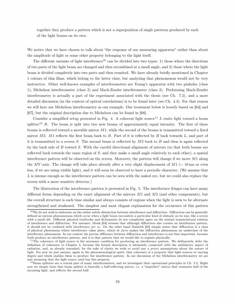
together they produce a pattern which is not a superposition of single patterns produced by each

of the light beams on its own.

We notice that we have chosen to talk about “the response of our measuring apparatus” rather than about

the amplitude of light or some other property belonging to the light itself.

The different variants of light interference10 can be divided into two types: 1) those where the directions

of two parts of the light beam are changed and then recombined at a small angle, and 2) those where the light

beam is divided completely into two parts and then reunited. We have already briefly mentioned in Chapter

1 colours of thin films, which belong to the latter class, but analyzing that phenomenon would not be very

instructive. Other well-known examples of interferometers are Young’s apparatus with two pinholes (class

1), Michelson interferometer (class 2) and Mach-Zender interferometer (class 2). Performing Mach-Zender

interferometry is actually a part of the experiment associated with the thesis (see Ch. 7.2), and a more

detailed discussion (in the context of optical correlations) is to be found later (see Ch. 4.4). For that reason

we will here use Michelson interferometry as our example. Our treatment below is loosely based on [64] and

[67], but the original description due to Michelson can be found in [68].

Consider a simplified setup presented in Fig. 4. A coherent light source11 L emits light toward a beam

splitter12 B. The beam is split into two new beams of approximately equal intensity. The first of these

beams is reflected toward a movable mirror M1, while the second of the beams is transmitted toward a fixed

mirror M2. M1 reflects the first beam back to B. Part of it is reflected by B back towards L, and part of

it is transmitted to a screen S. The second beam is reflected by M2 back to B and then is again reflected

by the back side of B toward S. With the careful directional alignment of mirrors (so that both beams are

reflected back towards the same region of S, and they make a small angle relatively to each other), a spatial

interference pattern will be observed on the screen. Moreover, the pattern will change if we move M1 along

the MY -axis. The change will take place already after a very slight displacement of M1 (∼ 10 nm or even

less, if we are using visible light), and it will soon be observed to have a periodic character. (We assume that

L is intense enough so the interference pattern can be seen with the naked eye, but we could also replace the

screen with a more sensitive detector.)

The illustration of the interference pattern is presented in Fig. 5. The interference fringes can have many

different forms depending on the exact alignment of the mirrors M1 and M2 (and other components), but

the overall structure is each time similar and always consists of regions when the light is seen to be alternate

strengthened and weakened. The simplest and most elegant explanation for the occurence of this pattern10We do not wish to elaborate on the rather subtle distinction between interference and diffraction. Diffraction can be generally

defined as various phenomenona which occur when a light beam encounters a particular kind of obstacle on its way, like a screenwith a small slit. Different physical textbooks and dictionaries do not completely agree on the mutual nomenclatural relationof interference and diffraction. For instance, Monk [64] stresses that although diffraction also creates an interference pattern,it should not be confused with interference per se. On the other hand Daintith [65] simply states that diffraction is a classof physical phenomena where interference takes place, which de facto makes the diffraction phenomena an underclass of theinterference phenomena. In our context the precise difference between diffraction and interference is not that important, becauseboth produce an interference pattern, and it is that pattern that we would like to explain physically.

11The coherence of light source is the necessary condition for producing an interference pattern. We delibaretely defer thedefinition of coherence to Chapter 4, because the formal description is intimately connected with the undulatory aspect ofradiation, and, as already remarked, for the sake of clarity we wish to avoid any a priori assumptions about the nature oflight. For now we just assume, again in the phenomenological spirit, that coherence is a property that light sources in varyingdegree and which enables them to produce the interference pattern. In our discussion of the Michelson interferometry we arejust assuming that the light source used has this property.

12Beam splitters are a crucial part of many interferometers, and we investigate their operational principles in Ch. 5.2. Rightnow we simply state that beam splitter is basically a half-reflecting mirror, i.e. a “imperfect” mirror that transmits half of theincoming light, and reflects the second half.

34

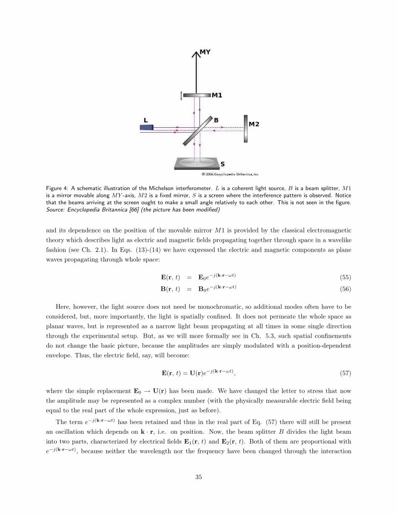
Figure 4: A schematic illustration of the Michelson interferometer. L is a coherent light source, B is a beam splitter, M1is a mirror movable along MY -axis, M2 is a fixed mirror, S is a screen where the interference pattern is observed. Noticethat the beams arriving at the screen ought to make a small angle relatively to each other. This is not seen in the figure.Source: Encyclopedia Britannica [66] (the picture has been modified)

and its dependence on the position of the movable mirror M1 is provided by the classical electromagnetic

theory which describes light as electric and magnetic fields propagating together through space in a wavelike

fashion (see Ch. 2.1). In Eqs. (13)-(14) we have expressed the electric and magnetic components as plane

waves propagating through whole space:

E(r, t) = E0e−j(k·r−ωt) (55)

B(r, t) = B0e−j(k·r−ωt) (56)

Here, however, the light source does not need be monochromatic, so additional modes often have to be

considered, but, more importantly, the light is spatially confined. It does not permeate the whole space as

planar waves, but is represented as a narrow light beam propagating at all times in some single direction

through the experimental setup. But, as we will more formally see in Ch. 5.3, such spatial confinements

do not change the basic picture, because the amplitudes are simply modulated with a position-dependent

envelope. Thus, the electric field, say, will become:

E(r, t) = U(r)e−j(k·r−ωt), (57)

where the simple replacement E0 → U(r) has been made. We have changed the letter to stress that now

the amplitude may be represented as a complex number (with the physically measurable electric field being

equal to the real part of the whole expression, just as before).

The term e−j(k·r−ωt) has been retained and thus in the real part of Eq. (57) there will still be present

an oscillation which depends on k · r, i.e. on position. Now, the beam splitter B divides the light beam

into two parts, characterized by electrical fields E1(r, t) and E2(r, t). Both of them are proportional with

e−j(k·r−ωt), because neither the wavelength nor the frequency have been changed through the interaction

35

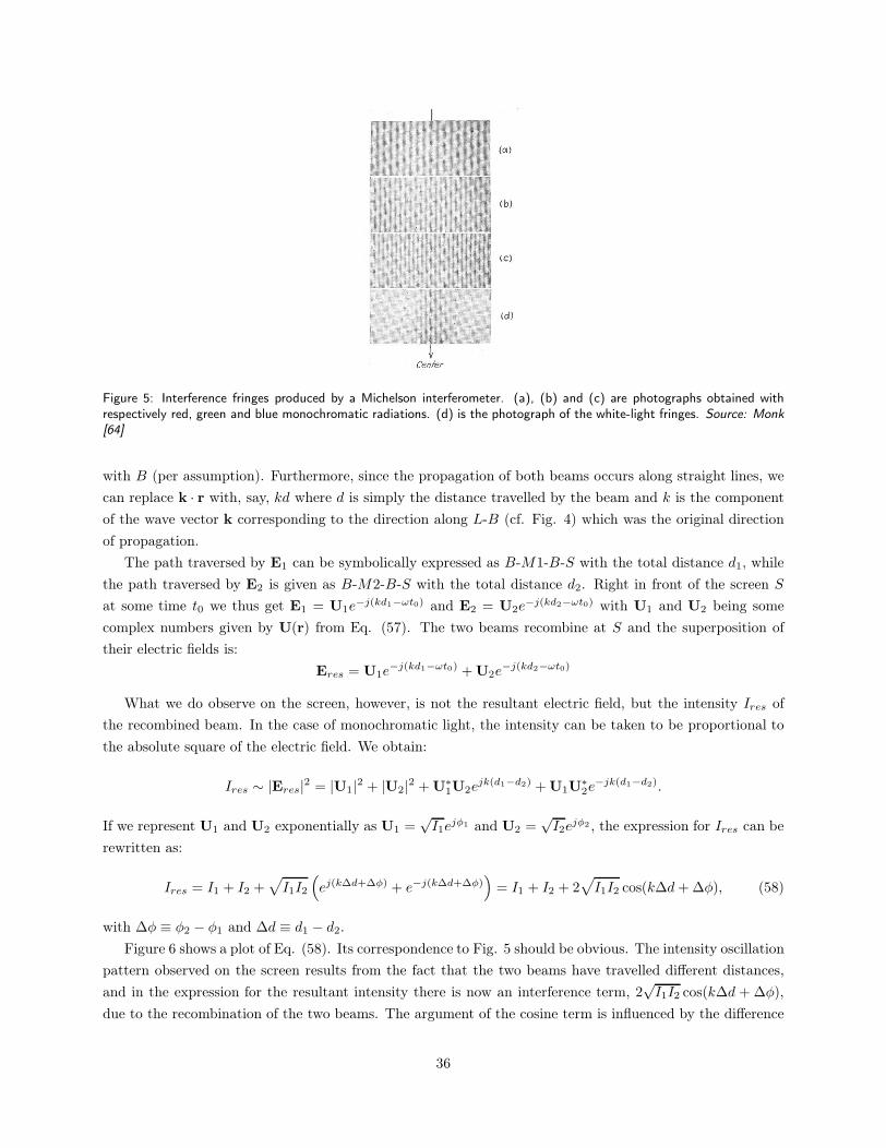
Figure 5: Interference fringes produced by a Michelson interferometer. (a), (b) and (c) are photographs obtained withrespectively red, green and blue monochromatic radiations. (d) is the photograph of the white-light fringes. Source: Monk[64]

with B (per assumption). Furthermore, since the propagation of both beams occurs along straight lines, we

can replace k · r with, say, kd where d is simply the distance travelled by the beam and k is the component

of the wave vector k corresponding to the direction along L-B (cf. Fig. 4) which was the original direction

of propagation.

The path traversed by E1 can be symbolically expressed as B-M1-B-S with the total distance d1, while

the path traversed by E2 is given as B-M2-B-S with the total distance d2. Right in front of the screen S

at some time t0 we thus get E1 = U1e−j(kd1−ωt0) and E2 = U2e

−j(kd2−ωt0) with U1 and U2 being some

complex numbers given by U(r) from Eq. (57). The two beams recombine at S and the superposition of

their electric fields is:

Eres = U1e−j(kd1−ωt0) + U2e

−j(kd2−ωt0)

What we do observe on the screen, however, is not the resultant electric field, but the intensity Ires of

the recombined beam. In the case of monochromatic light, the intensity can be taken to be proportional to

the absolute square of the electric field. We obtain:

Ires ∼ |Eres|2 = |U1|2 + |U2|2 + U∗1U2e

jk(d1−d2) + U1U∗2e

−jk(d1−d2).

If we represent U1 and U2 exponentially as U1 =√I1e

jφ1 and U2 =√I2e

jφ2 , the expression for Ires can be

rewritten as:

Ires = I1 + I2 +√

I1I2

(

ej(k∆d+∆φ) + e−j(k∆d+∆φ))

= I1 + I2 + 2√

I1I2 cos(k∆d+ ∆φ), (58)

with ∆φ ≡ φ2 − φ1 and ∆d ≡ d1 − d2.

Figure 6 shows a plot of Eq. (58). Its correspondence to Fig. 5 should be obvious. The intensity oscillation

pattern observed on the screen results from the fact that the two beams have travelled different distances,

and in the expression for the resultant intensity there is now an interference term, 2√I1I2 cos(k∆d + ∆φ),

due to the recombination of the two beams. The argument of the cosine term is influenced by the difference

36

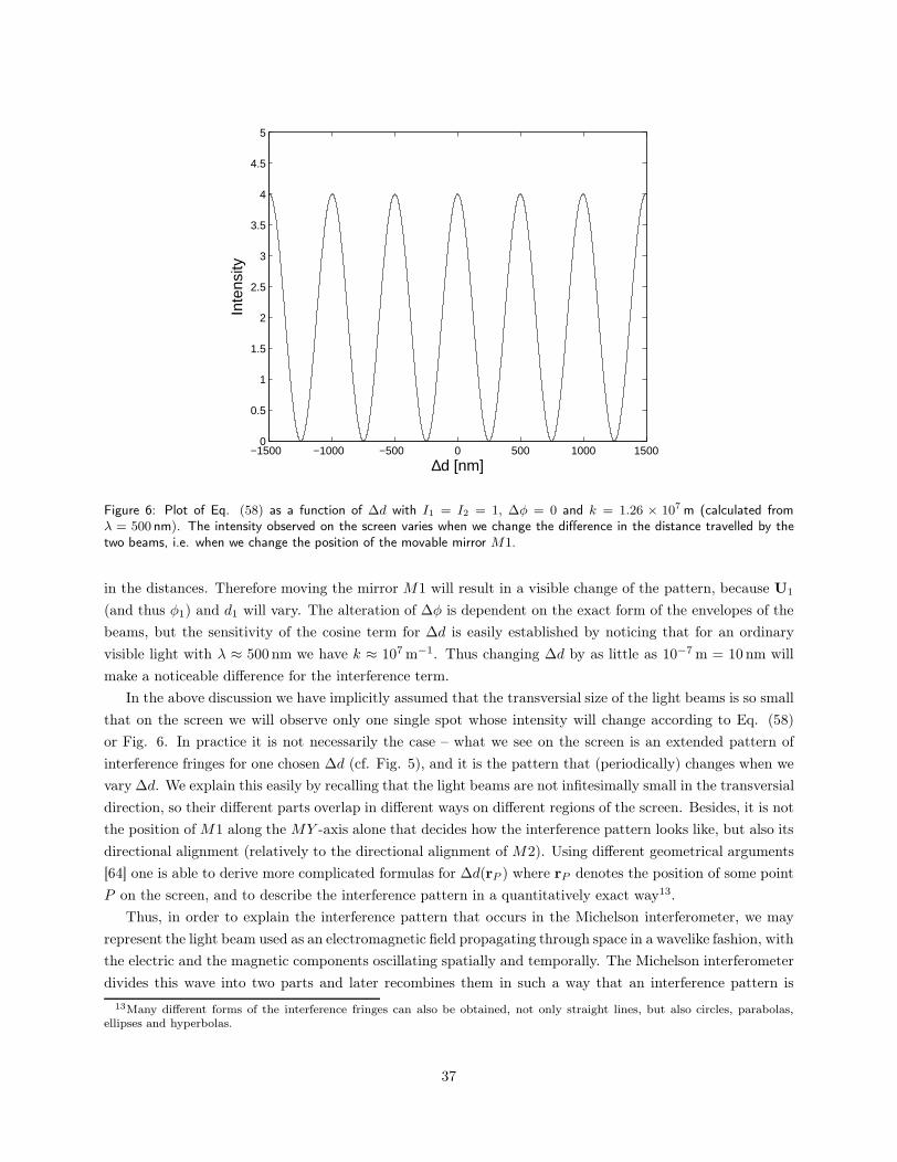
−1500 −1000 −500 0 500 1000 15000

0.5

1

1.5

2

2.5

3

3.5

4

4.5

5

∆d [nm]

Inte

nsity

Figure 6: Plot of Eq. (58) as a function of ∆d with I1 = I2 = 1, ∆φ = 0 and k = 1.26 × 107 m (calculated fromλ = 500 nm). The intensity observed on the screen varies when we change the difference in the distance travelled by thetwo beams, i.e. when we change the position of the movable mirror M1.

in the distances. Therefore moving the mirror M1 will result in a visible change of the pattern, because U1

(and thus φ1) and d1 will vary. The alteration of ∆φ is dependent on the exact form of the envelopes of the

beams, but the sensitivity of the cosine term for ∆d is easily established by noticing that for an ordinary

visible light with λ ≈ 500 nm we have k ≈ 107 m−1. Thus changing ∆d by as little as 10−7 m = 10 nm will

make a noticeable difference for the interference term.

In the above discussion we have implicitly assumed that the transversial size of the light beams is so small

that on the screen we will observe only one single spot whose intensity will change according to Eq. (58)

or Fig. 6. In practice it is not necessarily the case – what we see on the screen is an extended pattern of

interference fringes for one chosen ∆d (cf. Fig. 5), and it is the pattern that (periodically) changes when we

vary ∆d. We explain this easily by recalling that the light beams are not infitesimally small in the transversial

direction, so their different parts overlap in different ways on different regions of the screen. Besides, it is not

the position of M1 along the MY -axis alone that decides how the interference pattern looks like, but also its

directional alignment (relatively to the directional alignment of M2). Using different geometrical arguments

[64] one is able to derive more complicated formulas for ∆d(rP ) where rP denotes the position of some point

P on the screen, and to describe the interference pattern in a quantitatively exact way13.

Thus, in order to explain the interference pattern that occurs in the Michelson interferometer, we may

represent the light beam used as an electromagnetic field propagating through space in a wavelike fashion, with

the electric and the magnetic components oscillating spatially and temporally. The Michelson interferometer

divides this wave into two parts and later recombines them in such a way that an interference pattern is

13Many different forms of the interference fringes can also be obtained, not only straight lines, but also circles, parabolas,ellipses and hyperbolas.

37

produced. Mathematically, the most simple case of this procedure is given by Eq. (58). Descriptions of other

variants of interference (and diffraction) may be much more complicated (due to the complex geometry of

the given setting), but physically we can always assume the wavefronts of the two beams under consideration

superpose so that in some regions they reinforce themselves, and in some other regions they attenuate

themselves, these two occurences being called respectively constructive and destructive interference.

The wave picture of light (or, more generally, of electromagnetic radiation) allows thus to describe inter-

ference in an elegant and consistent manner. The corpuscular view of light, however, does not. Let us see

how far do we get with a heuristic approach. Imagine that our light source does not emit an electromagnetic,

continuous field, but a stream of minute light particles called photons, which are sharply localized energy

excitations travelling through space at the speed of light. The density of the stream is n photons per unit

length. Let us also assume that the screen S is photoluminescent, so when a photon hits it, a flash of light

is produced and our eyes register it. Now, the stream of photons meets first the beam splitter B on its way.

For each of the photons the beam splitter randomly decides if it should be sent (undivided, per definition of

the light quantum) towards M1 or M2 (the process of the beam splitting is examined in more detail in Ch.

5.2). Since the probability of sending a photon towards M1 is presumed to equal the probability of sending

it towards M2, we end up with two new streams of photons travelling in two different directions, each having

a density of approximately n2 (some stochastic fluctuations are allowed, but they are of no consequence for us

here). The mirrors reflect the two photon streams back to S, just like in the description of the interferometer

above. They recombine and interact with the photoluminescent screen.

Intuitively, the corpuscular view of light does not make us expect any particular pattern to arise on the

screen. If a single photon stream of density n would produce a light spot of intensity I on the photoluminescent

screen, then a single photon stream of density n2 should give14 a light spot of intensity I

2 . Now, if we divide

a single stream of density n into two equal parts, and then reunite them again and let the resultant beam

interact with the screen, we expect a uniform light spot of intensity I given by a formula similar to Eq. (58),

but without the interference term.

Empirically, however, we do obtain an interference pattern on the screen. Can it be explained using

photons? What comes immediately to mind is that the photons from the two beams could interact with

each other in some way, such that in some regions of the screen there arrives more of them than in some

other regions. If the photons are perceived as corpuscles, they could for instance scatter from each other and,

statistically, the scattering would result in a particular pattern observed on the screen. This line of thought

could be followed on, were it not for the dependence of the pattern on ∆d, the difference in distances travelled

by the two beams. Because of it, we are forced to assume that there is some specific property possessed by the

photon which changes as a function of the path length, and that this property is decisive for the manner in

which the photons from the two beams interact during their recombination into one stream and their arrival

upon the screen.

Were the photons ordinary physical particles, an obvious candidate for such a property would be velocity.

Namely, we could assume that the photons are gradually slowing down on their way from L to S. The

14 We assume here that the photons are identical. Also, their density in each case is so large that a flash of light produced

on the screen by a single photon does not have enough time to wane before the next photon hits the screen and a new flash of

photoluminescence is generated. Therefore the screen does not produce discrete flashes of light corresponding to each photon hit

separately, but instead we obtain an “accumulated” light spot with intensity proportional to the density of the incoming photon

stream.

38

velocity would without a doubt be a very important factor in determining how the two beams interact during

the recombination and what pattern is produced on the screen. However, a distinguished role of the velocity

is of course ruled out in this context, because the light is known to have the constant speed c.

Moreover, the property needs change in a periodic fashion, if we wish to be able to reproduce the ex-

perimental results. It is thus hard to see what kind of property could it be, if one does not want to resort

to the wave picture and to employ the phase. We could, however, try to equip the photon with some kind

of internal “clock” that measures the distance the photon has travelled or the time that has passed since its

emission15, and whose “hands” periodically return to the same values16, but this idea seems rather artificial.

The corpuscular picture of light not only has serious difficulties in explaining the interference pattern,

but it also leads us to an additional problem that touches the heart of the wave-particle paradox. Assume

that we represent the light as a stream of photons as before, and that each photon carries energy E given by

Planck’s formula E = ~ω, where ω is the angular frequency of the light, if the classical electromagnetic model

were to be applied. Let us again use visible monochromatic light with wavelength λ = 500 nm. A simple

calculation gives ω = 3.76 × 1015 s−1 and E ≈ 4 × 10−19 J. If the effect of the light source combined with

appropriate filters lies around 0.01 nW, the light source produces around 2.5 × 107photons per second, i.e.

approximately one photon each 4× 10−8 s. Let us make the size of the Michelson interferometer quite small,

so that the longest of the two possible photon paths does not exceed 50 cm. A photon propagating with the

speed of light needs only 1.6 × 10−9 s to traverse that distance, so we can safely assume that there is one

photon in the apparatus at any given time – if the light source emits photons with equal (or almost equal)

time intervals between two consecutive emissions (such regularity is formally described in the framework of

photon and photocount statistics which we will discuss in Sects. 5.1.2-5.1.3).

We have therefore affirmed – working still in the framework of the corpuscular model – that a single

photon is emitted from the light source, meets the beam splitter, is sent randomly towards either M1 or M2

(undivided), reflects back from one of the mirrors and after a fraction of nanosecond hits the photoluminescent

screen. Thus we do not expect any interference pattern depending on the distance difference ∆d, because

in the absence of two separate streams of photons continuously bombarding the screen there is apparently

no possibility for any inter-photon interactions that could lead to the creation of the pattern. Surprisingly

enough, an interference pattern of exactly the same kind as before will be still observed, although this time its

intensity will be understandably much smaller (because the intensity of the light source is now also very small),

and we will be possibly forced to use detectors more sensitive than a combination of the photoluminescent

screen and the naked eye.

The first observations of photonic self-interference in experimentally certain conditions are due to L.

Jánossy who conducted appropriate measurements in Budapest in the 1950s [70]. Jánossy used monochro-

matic radiation with wavelength 546.1 nm and coherence length of approximately 1 m. The arm length of

the Michelson interferometer employed was 14 m, and the total optical path for a photon traversing the

apparatus was 30 m long. With intensity as low as ca. 104 photons emitted per second Jánossy was confident

that only one photon was present in the interferometer at any given time17. The interference pattern was

15One could oppose such hypothesis by saying that, since the photon moves with the speed of light, its proper time is zero,and all lengths as measured from the “vantage point” of the photon are contracted to zero as well. The existence of such a“clock” would then be at odds with the special theory of relativity. Notice, however, that in the case of a wave of light, theposition- and time-dependant phase of the wave plays a role equivalent to that of the postulated “clock”, and no objections areraised in that case.

16Actually, this is the approach embraced by Richard Feynman in his popular presentation of quantum electrodynamics [69].17This crucial point was, however, criticized by Panarella [71]. According to Panarella Janossy had not presented a conclusive

proof that the photons were indeed isolated within the interferometer when they traversed it. Janossy should have reduced

39

observed, and Jánossy had to conclude that “interference phenomena are perfectly normal even at such low

intensities where at one time in average less than one photon is to be found in the arrangement; this is true

even if the dimensions of the arrangement greatly exceed the coherence length of the photons giving rise to

the patterns” [72].

The presence of the interference pattern in the case of single-photon interferometry leads us then easily to

believe that the concept of the corpuscular nature of light is erroneous, and that light should be represented

as an electromagnetic wave, even when the light source operates at very small intensities. This wave has then

very small amplitude indeed, but it is nonetheless divided by the beam splitter and thereafter both parts get

recombined, producing the interference fringes on the screen. This postulate could be verified by placing two

detectors, D1 and D2, instead of the two mirrors M1 and M2, and letting them measure incoming light in

coincidence. Unfortunately, results of such coincidence measurements – when conducted on classical states

of light (generated by thermal sources and lasers) – are ambiguous, as we will see in our analysis in Chapter

7.1. However, in case of nonclassical states of light an appropriate experiment was conducted by Clauser [73],

and the detectors worked indeed in anticoincidence, substantiating the corpuscular view of light.

An experiment similar to that of Clauser will be reviewed in Chapter 3.5, and in Section 5.1.4 we will

summarize the differences between classical and nonclassical states of light. Then we will come back again

to the issue of (anti)coincidence measurements in the context of our experiment in Chapter 7.1. In Chapter

7.2 the interference at the single photon level will be discussed again. For now we conclude that the classical

electromagnetic theory elegantly deals with the development of the interference patterns, and that occurence

of these patterns at very low intensities of light indicates that the theory, or at least some central elements

of it, remains valid in this regime.

3.3 The photoelectric effect

The photoelectric effect is the phenomenon where electrons are emitted from matter under an influence of

electromagnetic radiation18. In Chapter 1 we presented its historical context, and now we will proceed to

discuss the physical underpinnings of the phenomenon. In general terms it is easy to explain: A single electron

is initially bound in the material with energy E0 < 0, but it can absorb energy ER from the radiation. If

E0 +ER is larger than zero, the electron frees itself from the potential well and is emitted from the material

with the maximal kinetic energy equal to ER − |E0|.In the classical electromagnetic theory the energy flux (energy per second per meter squared) of an

electromagnetic field is given by the Poynting vector S :

S =1

µE× B,

where µ is the magnetic permeability and E and B vectorial quantities representing, respectively, the electric

further the intensity of light I and increased the counting time of the detector ∆t in such a way that the product I∆t wasconstant. If the interference pattern remained the same, it would demonstrate that the phenomenon is linear with light intensity,and the association of wave properties with a single particle would be substantiated. Otherwise one would discover that thereis a regime of even lower intensity where the detector was unable to discern any interference pattern, and that the assumptionabout one photon being present in the apparatus at any time was wrong.

18This in fact the external photoelectric effect. The difference between the external and the internal photoelectric effects isexplained in Chapter 5.1.

40

and the magnetic field (see Ch. 2.1). Thus the absolute value of the energy flux, |S|, seems to depend only

on the intensities of the component fields. We could then deduce that the emission of the electrons depends

on these intensities alone. However, experimental results due to Philipp Lenard [74] showed that this is not

the case, and that actually the frequency of the radiation plays an additional and essential role.

If, given a monochromatic radiation, the frequency is below some material-dependent value, no emission

of electrons will take place, even if we increase the intensity further19. But if the frequency exceeds the

threshold, then the emission will occur, even if the intensity remains low. Raising the frequency further will

result in the increase of the speed of the photoelectrons (the emitted electrons), while raising the intensity

will lead to more frequent emissions. In other words, the radiation frequency determines the kinetic energy

of the photoelectrons, while the radiation intensity determines their number, i.e. the photocurrent.

Using Lenard’s results Albert Einstein set out to explain the role of the frequency [31]. Einstein assumed

that the incident light of frequency ν consists of energy quanta, each with energy E given by Planck’s formula

E = hν. A light quantum interacts with a single electron in the material and transfers all energy to the

electron20. Let us denote by W the minimum energy needed remove an electron from a solid to a point

immediately outside the solid surface (the so-called work function). If E is larger than W , the electron leaves

the material with maximal kinetic energy Tν given simply by:

Tν = hν −W. (59)

The formula reproduced Lenard’s results to order of magnitude, and today the above explanation is taken

to be the standard physical intepretation of the photoelectric effect. Fig. 7 presents exemplary experimental

data describing the photoelectric effect, but since the original results of Lenard were unavailable for the

author of the thesis, the data measured by Owen Richardson and K. T. Compton in 1912 [75] have been

chosen instead.

We ask whether it is really necessary to assume the granular structure of light in order to give the physical

reason for the photoelectric effect and the associated experimental data. From an intuitive point of view the

conclusion of Einstein (that the light consists of energy quanta) may seem somewhat far-fetched, because

all we need do is to quantize the interaction between electromagnetic radiation and matter (more precisely,

the transfer of the energy from radiation to matter). Therefore we may ask whether it is possible to deduce

Eq. (59) in some alternative way which does not make an explicit use of the concept of photon. Given that

the approach of Einstein is taken for granted in almost every presentation of the photoelectric effect, it may

seem surprising that the answer is positive [76].

As early as in 1912 Owen Richardson derived Eq. (59) without resorting directly to the corpuscular view

of light (which at that time went under the name of “the unitary hypothesis”) [32] [77]. Richardson based

his model on statistical and thermodynamical principles combined with the laws of classical electrodynamics.

In his approach the photoemission process might be compared with evaporation from a liquid surface and

work function with latent heat of vaporization. Richardson considered a body being in thermal equilibrium

with the surrounding radiation of temperature θ, and examined how the radiative energy will be divided

among the electrons in the body. Now, if one electron acquires enough energy, it will be ejected. Richardson

19The emission may occur, however, if the intensity will become very large. This is the so-called anomalous photoelectriceffect, and we will shortly discuss it in the closing paragraphs of Sect. 9.1.3.

20Here we have to assume that multiple photons cannot interact with an electron at the same moment, and that the electronis not able to accumulate energy from different photons even if they interact with it rapidly one after another. Multiphotonscattering may occur, however, if the intensity is very large (see the previous footnote).

41

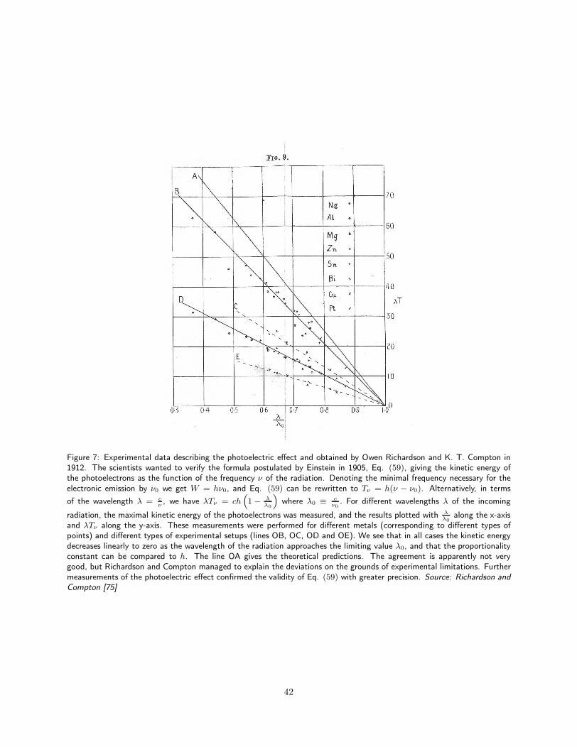
Figure 7: Experimental data describing the photoelectric effect and obtained by Owen Richardson and K. T. Compton in1912. The scientists wanted to verify the formula postulated by Einstein in 1905, Eq. (59), giving the kinetic energy ofthe photoelectrons as the function of the frequency ν of the radiation. Denoting the minimal frequency necessary for theelectronic emission by ν0 we get W = hν0, and Eq. (59) can be rewritten to Tν = h(ν − ν0). Alternatively, in terms

of the wavelength λ = cν, we have λTν = ch

“

1 − λλ0

”

where λ0 ≡ cν0

. For different wavelengths λ of the incoming

radiation, the maximal kinetic energy of the photoelectrons was measured, and the results plotted with λλ0

along the x-axisand λTν along the y-axis. These measurements were performed for different metals (corresponding to different types ofpoints) and different types of experimental setups (lines OB, OC, OD and OE). We see that in all cases the kinetic energydecreases linearly to zero as the wavelength of the radiation approaches the limiting value λ0, and that the proportionalityconstant can be compared to h. The line OA gives the theoretical predictions. The agreement is apparently not verygood, but Richardson and Compton managed to explain the deviations on the grounds of experimental limitations. Furthermeasurements of the photoelectric effect confirmed the validity of Eq. (59) with greater precision. Source: Richardson andCompton [75]

42

demonstrated that the number N of electrons emitted from unit area of the body may be expressed either

as the definite integral:

N =c

4

∫ ∞

0

ǫF (ν, θ)E(ν, θ) dν, (60)

or explicitly as:

N = αA√θ exp

(∫

w

kθ2dθ

)

. (61)

The symbols used has the following meanings: c is the speed of light, ν is the radiation frequency, ǫF (ν, θ) is

the number of electrons emitted in the presence of unit electromagnetic radiation with temperature θ whose

frequency lies between ν and ν+dν, E(ν, θ) is the spectral distribution of the electromagnetic energy density

(in equilibrium), α is the fraction of the returning electrons which are absorbed (i.e. not reflected), A is a

constant dependent on the material under consideration (but independent of θ), w is the internal latent heat

of evaporation of one electron and k is Boltzmann’s constant (in his treatment Richardson used R, the gas

constant for one molecule, instead of k; but k is per definition identical to the normalized gas constant).

Richardson, basing his reasoning on Eqs. (60) and (61), proceeded then to show how Eq. (59) will follow.

First, let us notice that the right-hand sides of the above equations have to be equal, so these can be combined

into a single integral equation true for all values of θ:

c

4

∫ ∞

0

ǫF (ν, θ)E(ν, θ) dν = αA√θ exp

(∫

w

kθ2dθ

)

. (62)

Since E(ν, θ), A, α and w are either known (the spectral distribution is given by Planck’s formula, and the

material and proportion constants are detemined from experiment) or can be approximated (the internal

latent heat), we would like to solve the equation for ǫF (ν, θ). Richardson assumed that

w = w0 +3

2kθ (63)

for some constant w0, and instead of using the ordinary Planck formula:

E(ν, θ) =8πhν3

c31

ehνkθ − 1

,

he simplified it to:

E(ν, θ) =8πhν3

c3e−

hνkθ , (64)

since the replacement only causes inaccuracies in the final result proportional to e−w0/kθ which is a very tiny

fraction except at high temperatures (larger than ca. 5000 K). Putting Eqs. (63) and (64) into (62) the

integral equation can be written as:

c

4

∫ ∞

0

ǫF (ν, θ) × 8πhν3

c3e−

hνkθ dν = αA

√θ exp

(∫

w0

kθ2dθ

)

exp

(∫

3

2θdθ

)

2π

c2

∫ ∞

0

ǫF (ν, θ)hν3e−hνkθ dν = αAθ2 exp

(−w0

kθ

)

∫ ∞

0

ǫF (ν, θ)hν3e−hνkθ dν = α

Ac2

2πθ2 exp

(−w0

kθ

)

(65)

43

Assuming that α = 1 (no reflection of the returning electrons), the above equation is satisfied by:

ǫF (ν, θ) = 0, if 0 < hν < w0 (66)

ǫF (ν, θ) =Ac2h

2πk2ν2

(

1 − w0

hν

)

, if w0 < hν <∞. (67)

We observe that if the frequency ν of the electromagnetic radiation is so small that the product hν is less

than w0 (which corresponds to the minimal energy required to free a single electron from its bounded state

in the material), no photoelectrons will be emitted at all. Only past this value ǫF (ν, θ) will be different from

zero. Moreover, we see that ǫF (ν, θ) is in fact independent of temperature, just like experiments indicate,

so we should rather express it as ǫF (ν). One might possibly argue that the solution to Eq. (65) contained

in Eqs. (66)-(67) is contrived in the sense that Eq. (65) has also other solutions without the discontinuity

at ν0 = w0

h . But this is not true – as Richardson showed, there is no single analytic function ǫF (ν, θ) that

solves the integral equation throughout the interval ν ∈ [0, ∞].

Choose now Tν to be the average kinetic energy of a photoelectron which is emitted from the material

due to radiation with frequency ν. The total energy E emitted is given by the integral:

E =c

4

∫ ∞

0

TνǫF (ν, θ)E(ν, θ) dν

One can show that the energy streaming towards the material in unit time by virtue of the thermal motion

of the external electrons is 2Nkθ. If 0 ≤ β ≤ 1 is the fraction of these electrons that are absorbed, we have

in equilibrium:

E = 2βNkθ.

By setting β = 1 (total absorption) and using Eq. (61) for N and Eq. (64), we end up with another integral

equation:2π

c2

∫ ∞

0

TνǫF (ν, θ)hν3e−hνkθ dν = 2αAkθ3/2 exp

(∫

w

kθ2dθ

)

.

With α = 1, w approximated as before and ǫF (ν, θ) given by the solution above, we can find the following

expression for Tν :

Tν = hν − w0, if w0 ≤ hν <∞, (68)

Tν having no meaning if hν < w0, because then no photoelectrons are emitted. Thus, also here we have

derived the correct (from the experimental point of view) formula for the kinetic energy of a photoelectron

“without making use of the hypothesis that free radiant-energy exists in the form of “Licht-quanten,” unless

this hypothesis implicitly underlies the assumptions: (A) that Planck’s formula radiation is true; (B) that,

ceteris paribus, the number of electrons emitted is proportional to the intensity of monochromatic radiation”

[75]. Of course, we can conveniently explain Eq. (68) in terms of electromagnetic radiation consisting of

photons, but from a formal point of view the notion of quantized light is not necessary in order to deduce

this formula. However, we do have to make use of Planck’s results and the constant h which suggest that

the energy exchange between light and matter is somehow quantized. Still, this does not prevent us from

perceiving light as such as a continuous electromagnetic wave.

Although the form of Eq. (68) with the discontinuity at ν = w0

h is not a reason strong enough to fully

accept Einstein’s hypothesis, we can in addition consider the principle of the energy conservation in the case

of the photoelectric effect. Assume that we use electromagnetic radiation – perceived, to begin with, as a

44

wave and described classically by Poynting vector S – to irradiate a material with an area described by vector

A. Assume also that in order to make the material emit a single photoelectron we need supply it energy E0

(i.e. this is the work function). This energy will be delivered from the radiation to the material after time T

given by the equation:∫ T

0

dt

∫

A

S·dA = E0,

if we assume that the irradiation started at time t = 0. Now, we could experimentally measure Tmin, the

minimum time between the beginning of the irradiation and the emission of the first photoelectron. If we

would find Tmin > T , it would show that the radiative energy flows into the metal in a continuous manner and

thus the undulatory view of light would be supported21. On the other hand, if we would find Tmin < T , we

would have to theoretically allow for the situation where the necessary energy E0 is delivered “immediately”

(or at least much quicker than the classical theory allows), and this is most easily explained in the virtue of

the corpuscular view, i.e. in the virtue of radiation travelling through space as discrete energy packets.

The experiment in question was conducted by C. E. Tyler [78] who found that Tmin < T . However,

his results were partially inconclusive, because in the setup for switching the light beam on and off he had

employed an electro-optical shutter which attenuated the beam ca. 200 times instead of shutting it off

completely. Davis and Mandel performed another version of Tyler’s experiment where they replaced the

electro-optical shutter with a mechanical one that allowed for a full stoppage of the light beam [79]. T was

assigned the value of 20µs. The reasoning based on the undulatory view predicted thus that no photoelectron

should be emitted for irradiation times shorter than 20µs, no more than one photoelectron should be emitted

for irradiation times shorter than 40µs, etc. However, Davis and Mandel found both that Tmin < T and

that the probability distribution P (n, τ) for emission of n photoelectrons during the irradiation time τ was

actually independent of τ (Fig. 8).

These results were taken as a proof for the corpuscular view of light. However, we observe that several

loopholes remained. In the first place, the minimal resolution in the experiment was 5 µs, so the experiment

did not substantiate the claim that energy transfer was instantaneous. All that could be said with certainty

was that this transfer took 5 µs or less. Secondly, it was conceivable that fluctuations were present in the

electromagnetic field on the time scale of 5 µs, and that their intensity was occasionally high enough to

excite photoelectrons before the “required” 20 µs have passed. In other words, one could argue that the

short-time (< 5 µs) average of the energy transmitted by the wave was not necessarily equal to the long-

time (> 5 µs) average. Thirdly, Davis and Mandel postulated that each electron was characterized by the

same work function E0. This assumption was an idealization, since the material consisted of a very large

amount of electrons, so their work functions might somewhat vary. Alternatively one could point out that the

authors did not irradiate single and separated electrons having fixed binding energy, but rather a complicated

solid-state structure consisting of many electrons and atoms. E0 was thus an average value.

We see that the basic features of the photoelectric effect do not – as is often dogmatically claimed in

textbooks – force upon us the corpuscular view of light, because the well-known formula given by Eq. (68)

can be deduced without resorting to that view explicitly. The consideration of the energy conservation law

presents us with additional questions, so it would be interesting to repeat Davis and Mandel’s experiment

21We should stop here and ask how the continuous flow of energy could be reconciled with the aforementioned quantizedenergy exchange between light and matter. After all, even if Tmin is indeed found to be larger than T , Eq. (68) is still validand the constant h stems from the Planck theory which implicitly postulates some kind of energy discretization. However,this discretization could be attributed to the irradiated material alone (i.e. to the discrete excitation of photoelectrons) as thesemiclassical model of photodetection demonstrates (see Sect. 5.1.2).

45

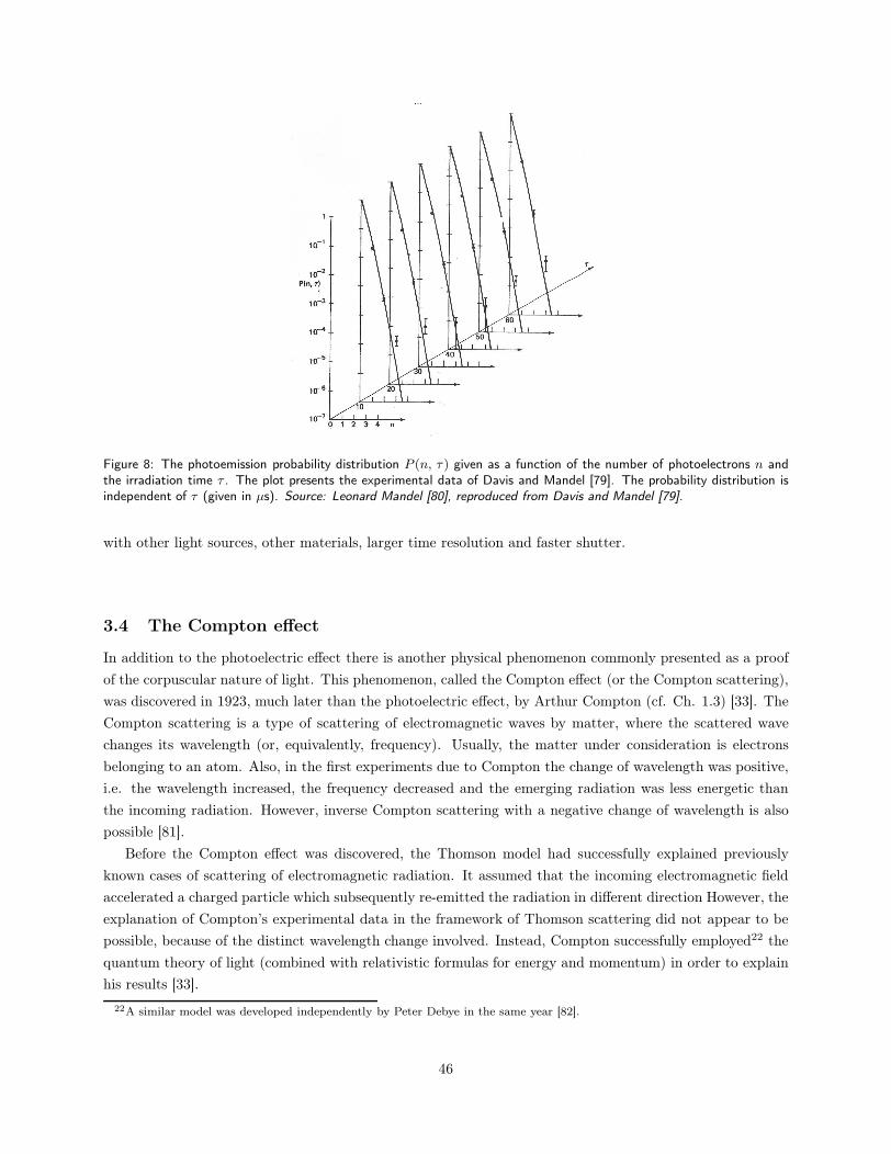
Figure 8: The photoemission probability distribution P (n, τ ) given as a function of the number of photoelectrons n andthe irradiation time τ . The plot presents the experimental data of Davis and Mandel [79]. The probability distribution isindependent of τ (given in µs). Source: Leonard Mandel [80], reproduced from Davis and Mandel [79].

with other light sources, other materials, larger time resolution and faster shutter.

3.4 The Compton effect

In addition to the photoelectric effect there is another physical phenomenon commonly presented as a proof

of the corpuscular nature of light. This phenomenon, called the Compton effect (or the Compton scattering),

was discovered in 1923, much later than the photoelectric effect, by Arthur Compton (cf. Ch. 1.3) [33]. The

Compton scattering is a type of scattering of electromagnetic waves by matter, where the scattered wave

changes its wavelength (or, equivalently, frequency). Usually, the matter under consideration is electrons

belonging to an atom. Also, in the first experiments due to Compton the change of wavelength was positive,

i.e. the wavelength increased, the frequency decreased and the emerging radiation was less energetic than

the incoming radiation. However, inverse Compton scattering with a negative change of wavelength is also

possible [81].

Before the Compton effect was discovered, the Thomson model had successfully explained previously

known cases of scattering of electromagnetic radiation. It assumed that the incoming electromagnetic field

accelerated a charged particle which subsequently re-emitted the radiation in different direction However, the

explanation of Compton’s experimental data in the framework of Thomson scattering did not appear to be

possible, because of the distinct wavelength change involved. Instead, Compton successfully employed22 the

quantum theory of light (combined with relativistic formulas for energy and momentum) in order to explain

his results [33].

22A similar model was developed independently by Peter Debye in the same year [82].

46

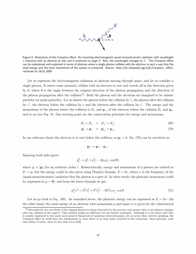
Figure 9: Illustration of the Compton effect: An incoming electromagnetic quasi-monochromatic radiation with wavelengthλ interacts with an electron at rest and is scattered to angle θ. Also, the wavelength changes to λ

′

. The Compton effectcan be understood and explained in terms of photons where a single photon collides with the electron in such a way that thetotal energy and the total momentum of the system is conserved. Source: http://en.wikipedia.org/wiki/Compton_effect,retrieved on 26.01.2009

Let us represent the electromagnetic radiation as photons moving through space, and let us consider a

single photon. It enters some material, collides with an electron at rest and travels off in the direction given

by θ, where θ is the angle between the original direction of the photon propagation and the direction of

the photon propagation after the collision23. Both the photon and the electrons are imagined to be minute

particles (or point particles). Let us denote the photon before the collision by γ, the photon after the collision

by γ′

, the electron before the collision by e and the electron after the collision by e′

. The energy and the

momentum of the photon before the collision is Eγ and pγ , of the electron before the collision Ee and pe,

and so on (see Fig. 9). Our starting point are the conservation principles for energy and momentum:

Eγ + Ee = Eγ′ + Ee′ (69)

pγ + pe = pγ′ + pe′ . (70)

In our reference frame the electron is at rest before the collision, so pe = 0. Eq. (70) can be rewritten as:

pe′ = pγ − pγ′ .

Squaring both sides gives:

p2e′ = p2

γ + p2γ′ − 2pγpγ′ cos(θ),

where pi ≡ |pi| for an arbitrary index i. Relativistically, energy and momentum of a photon are related as

E = cp, but the energy could be also given using Planck’s formula, E = hν, where ν is the frequency of the

(quasi-monochromatic) radiation that the photon is a part of. In other words, the photonic momentum could

be expressed as p = hνc , and from the above formula we get:

p2e′ c2 = h2ν2

γ + h2ν2γ′ − 2h2νγνγ′ cos θ. (71)

Let us go back to Eq. (69). As remarked above, the photonic energy can be expressed as E = hν. On

the other hand, the total energy of an electron with momentum p and mass m is given by the relativistical

23Alternatively one can think of the original photon as being destroyed in the process, and assume that a new photon emergesafter the collision at the angle θ. This subtlety makes no difference for our further treatment. Although it is the latter view thatis usually employed in the much more general framework of quantum electrodynamics, let us notice that, strictly speaking, theCompton effect by itself does not substantiate it, since there is no time delay involved in the scattering. More precisely, suchtime delay, if exists, must be less than 0.5ns [83].

47

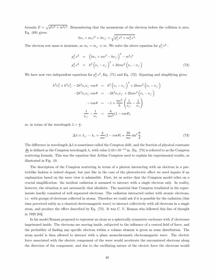
formula E =√

p2c2 +m2c4. Remembering that the momentum of the electron before the collision is zero,

Eq. (69) gives:

hνγ +mec2 = hνγ′ +

√

p2e′ c2 +m2

e′c4.

The electron rest mass is invariant, so me = me′ ≡ m. We solve the above equation for p2e′ c2 :

p2e′ c2 =

(

hνγ +mc2 − hνγ′

)2

−m2c4

p2e′ c2 = h2

(

νγ − νγ′

)2

+ 2hmc2(

νγ − νγ′

)

(72)

We have now two independent equations for p2e′ c2, Eq. (71) and Eq. (72). Equating and simplifying gives:

h2ν2γ + h2ν2

γ′ − 2h2νγνγ′ cos θ = h2(

νγ − νγ′

)2

+ 2hmc2(

νγ − νγ′

)

−2h2νγνγ′ cos θ = −2h2νγνγ′ + 2hmc2(

νγ − νγ′

)

− cos θ = −1 +mc2

h

(

1

νγ′

− 1

νγ

)

1

νγ′

− 1

νγ=

h

mc2(1 − cos θ),

or, in terms of the wavelength λ = cν :

∆λ ≡ λγ′ − λγ =h

mc(1 − cos θ) =

2h

mcsin2 θ

2. (73)

The difference in wavelength ∆λ is sometimes called the Compton shift, and the fraction of physical constantsh

mc is defined as the Compton wavelength λc with value 2.43×10−13 m. Eq. (73) is referred to as the Compton

scattering formula. This was the equation that Arthur Compton used to explain his experimental results, as

illustrated in Fig. 10.

The description of the Compton scattering in terms of a photon interacting with an electron in a par-

ticlelike fashion is indeed elegant, but just like in the case of the photoelectric effect we need inquire if an

explanation based on the wave view is admissible. First, let us notice that the Compton model relies on a

crucial simplification: the incident radiation is assumed to interact with a single electron only. In reality,

however, the situation is not necessarily that idealistic. The material that Compton irradiated in his exper-

iments hardly consisted of well separated electrons. The radiation interacted rather with atomic electrons,

i.e. with groups of electrons collected in atoms. Therefore we could ask if it is possible for the radiation (this

time perceived solely as a classical electromagnetic wave) to interact collectively with all electrons in a single

atom, and produce the effect described by Eq. (73). It was C. V. Raman who followed this line of thought

in 1928 [84].

In his model Raman proposed to represent an atom as a spherically symmetric enclosure with Z electrones

imprisoned inside. The electrons are moving inside, subjected to the influence of a central field of force, and

the probablity of finding any specific electron within a volume element is given as some distribution. The

atom model is then allowed to interact with a plane monochromatic electromagnetic wave. The electric

force associated with the electric component of the wave would accelerate the encountered electrons along

the direction of the component, and due to the oscillating nature of the electric force the electrons would

48

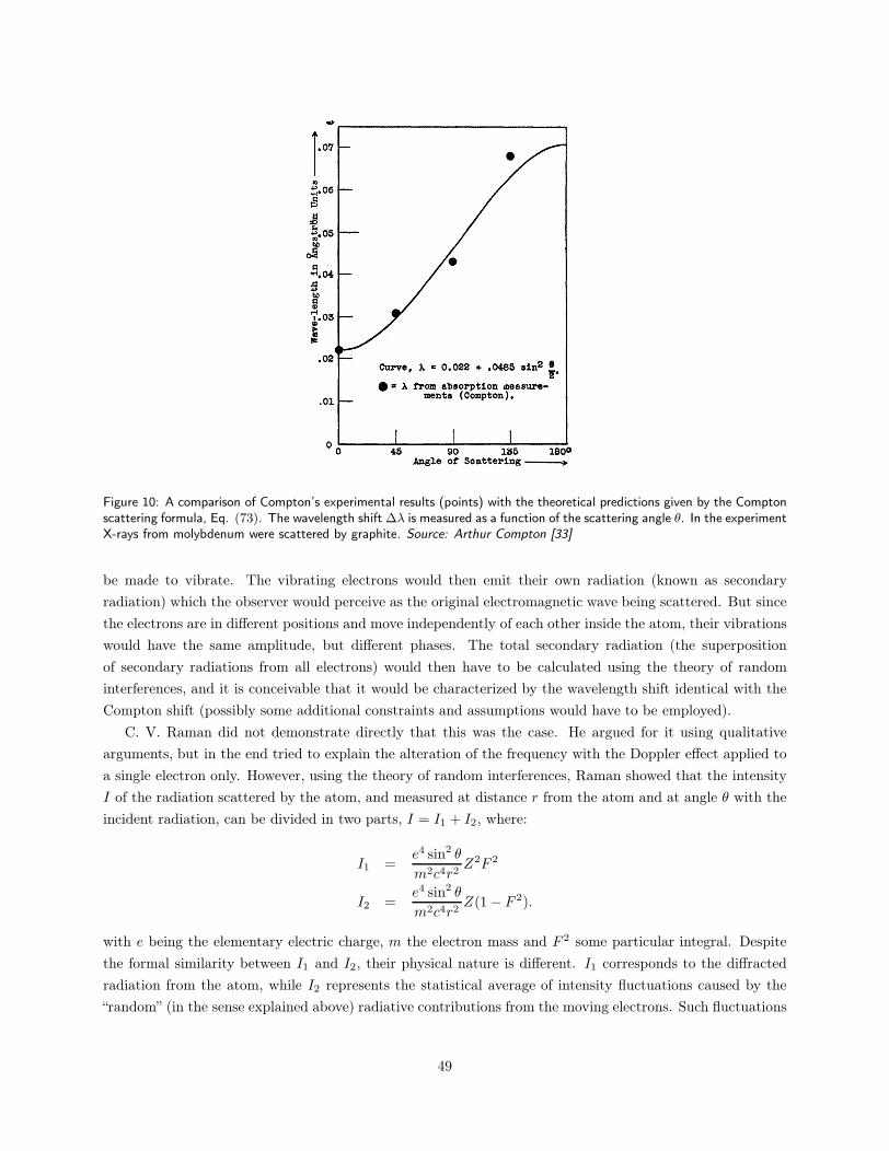
Figure 10: A comparison of Compton’s experimental results (points) with the theoretical predictions given by the Comptonscattering formula, Eq. (73). The wavelength shift ∆λ is measured as a function of the scattering angle θ. In the experimentX-rays from molybdenum were scattered by graphite. Source: Arthur Compton [33]

be made to vibrate. The vibrating electrons would then emit their own radiation (known as secondary

radiation) which the observer would perceive as the original electromagnetic wave being scattered. But since

the electrons are in different positions and move independently of each other inside the atom, their vibrations

would have the same amplitude, but different phases. The total secondary radiation (the superposition

of secondary radiations from all electrons) would then have to be calculated using the theory of random

interferences, and it is conceivable that it would be characterized by the wavelength shift identical with the

Compton shift (possibly some additional constraints and assumptions would have to be employed).

C. V. Raman did not demonstrate directly that this was the case. He argued for it using qualitative

arguments, but in the end tried to explain the alteration of the frequency with the Doppler effect applied to

a single electron only. However, using the theory of random interferences, Raman showed that the intensity

I of the radiation scattered by the atom, and measured at distance r from the atom and at angle θ with the

incident radiation, can be divided in two parts, I = I1 + I2, where:

I1 =e4 sin2 θ

m2c4r2Z2F 2

I2 =e4 sin2 θ

m2c4r2Z(1 − F 2).

with e being the elementary electric charge, m the electron mass and F 2 some particular integral. Despite

the formal similarity between I1 and I2, their physical nature is different. I1 corresponds to the diffracted

radiation from the atom, while I2 represents the statistical average of intensity fluctuations caused by the

“random” (in the sense explained above) radiative contributions from the moving electrons. Such fluctuations

49

are indeed observed during the Compton scattering, and the Raman’s model allows to understand their nature.

The Compton shift, however, is not rigorously deduced from the random interference assumption.

Still, let us see how the Doppler effect can be used to explain the Compton scattering when we limit our

attention to an interaction with a single electron. The generalized Doppler shift of light in the relativistic

framework is described by the formula:

λ′

= λ1 − v

c cosα√

1 − v2

c2

,

where λ is the emitted wavelength (as measured in the rest frame of the emitter), λ′

is the observed wave-

length, v is the speed of the emitter (as measured by the observer) and α is the angle between the direction

of light toward the observer and the velocity of the emitter. We consider now the situation illustrated in

Fig. 9. First, we consider the incoming radiation from the vantage point of the electron. We assume that

the electron recoils in the direction of propagation of the incident light24, so α = π and the above formula

simplifies to:

λ′

= λ1 + v

c√

1 − v2

c2

, (74)

where λ′

is the wavelength received by the electron recoiling with speed v. Now the electron becomes the

emitter and scatters the radiation in the direction given by θ (cf. Fig. 9). The scattered wavelength λ′′

is

measured to be:

λ′′

= λ′ 1 − v

c cosα√

1 − v2

c2

= λ

(

1 + vc

) (

1 − vc cos θ

)

1 − v2

c2

.

We calculate the wavelength shift:

∆λ = λ′′ − λ = λ

vc (1 − cos θ)

1 − vc

(75)

Kidd, Ardini and Anton [85] noticed that Eq. (75) is identical to Eq. (73) if λvc (1 − v

c )−1 = hmc and

argued that this similarity has to be something more than a mere coincidence. Their paper was stimulated

by an article due to Mellen [86] which had demonstrated how the equivalence between both formulas might

be achieved, if one applied the de Broglie hypothesis (see Appendix C). Let us express Eq. (75) in terms of

λ′ (given by Eq. (74)) which is the wavelength of the incident light as measured from the point of view of

the electron:

∆λ = λ′

vc

√

1 − v2

c2

(1 − cos θ).

In the classical model λ′

would be the wavelength of the oscillations of the electron as measured in its own

reference frame. But if we now assume that this is also de Broglie wavelength of the electron when influenced

by the external radiation, we get through Eq. (205) (see Appendix C):

∆λ =h

p×

vc

√

1 − v2

c2

(1 − cos θ) =h

mc(1 − cos θ),

since the momentum p is (relativistically) given as p = mv(

1 − v2

c2

)− 12

with m being the electron rest mass.

24It can be argued that this will happen on average; furthermore, this is the limiting value for the recoil direction when theCompton wavelength is much greater than the wavelength of the incident radiation, cf. [85].

50

Thus we obtain again the Compton formula, Eq. (73).

Incorporating de Broglie relationship into the alternative model for Compton scattering demands a proper

justification. It would be of course wrong to imagine an electron as a point particle oscillating due to the

incident radiation, and then blindly apply Eq. (205) in order to obtain the Compton scattering formula in

the end. We are rather forced to think in terms of de Broglie wave from the beginning. In this scheme the

electron is not a corpuscle, but a physical object of some kind represented as a wave in accordance with Eqs.

(205)-(206). This electron-object interacts with the incident radiation and scatters it, while recoiling itself

with speed v. However, in order for the scattering to occur with maximal efficiency, de Broglie wavelength of

the electron has to equal the wavelength of the incident radiation. This suggests that some kind of resonance

has to take place in the system. Otherwise the intensity of the scattered radiation ought to be reduced, i.e.

given a (quasi-)monochromatic incident radiation with wavelength λ1, the scattered radiation measured at

angle θ should have a maximum at λ2 (as given by Eq. (73)), but also should be broadened about it. Such

effect is indeed observed, but usually it is interpreted solely as Doppler broadening caused by the motion of

the target electrons [87].

The Compton effect, together with the photoelectric effect examined in the previous subsection, are today

frequently presented as main experimental pillars of the photon theory of light. In the historical context it

was the Compton effect – the combination of the experimental data obtained by Compton in 1923 and his

derivation of Eq. (73) – that forced many skeptics to accept the photon hypothesis. However, just as in the

case of the photoelectric effect, we have seen that it is not necessary to assume the corpuscular nature of

light in order to understand the origin of the Compton scattering formula. Specifically, instead of assuming

the corpuscular nature of both the incident radiation and the electron, we could as well interpret both the

radiation and the electron as waves (the latter as de Broglie wave). The presence of Planck’s constant h in

the resulting formula stems then directly from the de Broglie relations, Eqs. (205)-(206). However, it may

also suggest in addition that the energy transfer between the radiation and the electron has to be quantized

but, again as in the case of the photoelectric effect, the granular structure of light should not be considered

to be an inevitable consequence of the energy quantization scheme25.

3.5 The photon anticoincidence effect

The question of the nature of light is intimately connected with the photon anticoincidence effect. Consider

a radiative source which sends short, (quasi-)monochromatic outbursts of radiation. Let us assume that

we know with certainty that the radiation is not a continuous wave26, but we would like to experimentally

determine whether these outburst are inherently discrete (photons) or have a wave packet nature. Now, the

fundamental difference between the photons and the wave packets is that the photons, being energy quanta,

25Another derivation of Eq. (73) in which the radiation is described as classical electromagnetic waves can be found in Dodd[88]. Dodd does not resort to the idea of de Broglie waves and simply combines the Doppler effect with the assumption thatelectron energy changes discretely.

26Because if we would measure its intensity directly, we would find long periods of zero intensity separating short periodsof non-zero intensity. This is, per definition, the nature of the source employed. In practice performing such a measurementwith high accuracy could be difficult due to the various effects associated with the source, the detector and the backgroundradiation. Principially, however, the source could send high-intensity outbursts with large time intervals in between (relativelyto the temporal resolution of the detector), and this would minimize the uncertainty of the measurement.

51

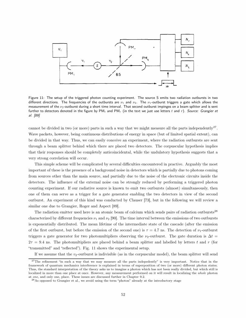
Figure 11: The setup of the triggered photon counting experiment. The source S emits two radiation outbursts in twodifferent directions. The frequencies of the outbursts are ν1 and ν2. The ν1-outburst triggers a gate which allows themeasurement of the ν2-outburst during a short time interval. That second outburst impinges on a beam splitter and is sentfurther to detectors denoted in the figure by PMt and PMr (in the text we just use letters t and r). Source: Grangier etal. [89]

cannot be divided in two (or more) parts in such a way that we might measure all the parts independently27.

Wave packets, however, being continuous distributions of energy in space (but of limited spatial extent), can

be divided in that way. Thus, we can easily conceive an experiment, where the radiation outbursts are sent

through a beam splitter behind which there are placed two detectors. The corpuscular hypothesis implies

that their responses should be completely anticoincidental, while the undulatory hypothesis suggests that a

very strong correlation will occur.

This simple scheme will be complicated by several difficulties encountered in practive. Arguably the most

important of these is the presence of a background noise in detectors which is partially due to photons coming

from sources other than the main source, and partially due to the noise of the electronic circuits inside the

detectors. The influence of the external noise can be strongly reduced by performing a triggered photon

counting experiment. If our radiative source is known to emit two outbursts (almost) simultaneously, then

one of them can serve as a trigger for a gate generator enabling the two detectors in view of the second

outburst. An experiment of this kind was conducted by Clauser [73], but in the following we will review a

similar one due to Grangier, Roger and Aspect [89].

The radiation emitter used here is an atomic beam of calcium which sends pairs of radiation outbursts28

characterized by different frequencies ν1 and ν2 [90]. The time interval between the emissions of two outbursts

is exponentially distributed. The mean lifetime of the intermediate state of the cascade (after the emission

of the first outburst, but before the emission of the second one) is τ = 4.7 ns. The detection of ν1-outburst

triggers a gate generator for two photomultipliers observing the ν2-outburst. The gate duration is ∆t =

2τ = 9.4 ns. The photomultipliers are placed behind a beam splitter and labelled by letters t and r (for

“transmitted” and “reflected”). Fig. 11 shows the experimental setup.

If we assume that the v2-outburst is indivisible (as in the corpuscular model), the beam splitter will send

27The refinement “in such a way that we may measure all the parts indepedently” is very important. Notice that in theframework of quantum mechanics interference is explained in terms of superposition of two (or more) different photon states.Thus, the standard interpretation of the theory asks us to imagine a photon which has not been really divided, but which still islocalized in more than one place at once. However, any measurement performed on it will result in localizing the whole photonat one, and only one, place. These issues are discussed further in Chapter 9.2.

28As opposed to Grangier et al., we avoid using the term “photon” already at the introductory stage

52

it either to t or to r; otherwise, it is possible that the two photomultipliers will register a coincidence. We

denote by N1 the rate of gates (the rate of the photon measurements by the gating detector), and by Nt and

Nr the separate (singles’) rates of t and r. Nc denotes the rate of coincident measurements by t and r. The

experimental results yield the probabilities pt and pr for singles’ counts during ∆t, and the probability pc for

coincidental counts during ∆t:

pt =Nt

N1, pr =

Nr

N1, pc =

Nc

N1.

Grangier et al. examined the theoretical relation between pc and the product of pt and pr, as given by the

classical electromagnetic description and by the quantum-mechanical formalism. The classical theory starts

with ascribing to the emitted ν2-outbursts a time-dependent intensity 2I(t) (the factor 2 is for convenience

only). If the beam splitter divides the outburst in two equal parts (with regard to the intensity), the time-

averaged intensity of one such part for the n-th gate is:

in =1

∆t

∫ tn+∆t

tn

I(t) dt,

where tn is the time at which the gate is opened. Choosing Ntot to be the total number of gates during the

experiment, the ensemble average of the time-averaged intensities is:

〈in〉 =1

Ntot

Ntot∑

n=1

in,

and the ensemble average of the time-averaged intensities squared is:

〈i2n〉 =1

Ntot

Ntot∑

n=1

i2n

The semiclassical model of photodetection (cf. Mandel and Wolf [55], p. 447) yields:

pt = ǫt∆t〈in〉, pr = ǫr∆t〈in〉, pc = ǫtǫr(∆t)2〈i2n〉, (76)

with ǫt and ǫr being the total detection efficiencies of t and r. Now, we have:

〈i2n〉 ≥ 〈in〉2

due to the Cauchy-Schwarz inequality. Thus we see that:

pc ≥ ptpr,

which means that the probability for a “real” coincidence (i.e. a situation where a divided radiation outburst

was registered simultaneously at both detectors) is at least as large as the probability for a “accidental”

coincidence (i.e. a situation where two different radiation outbursts were registered). The relation above can

be written as:

α ≡ pc

ptpr=NcN1

NtNr≥ 1. (77)

This is the prediction of the classical theory, or, more specifically, the prediction based on the four assump-

53

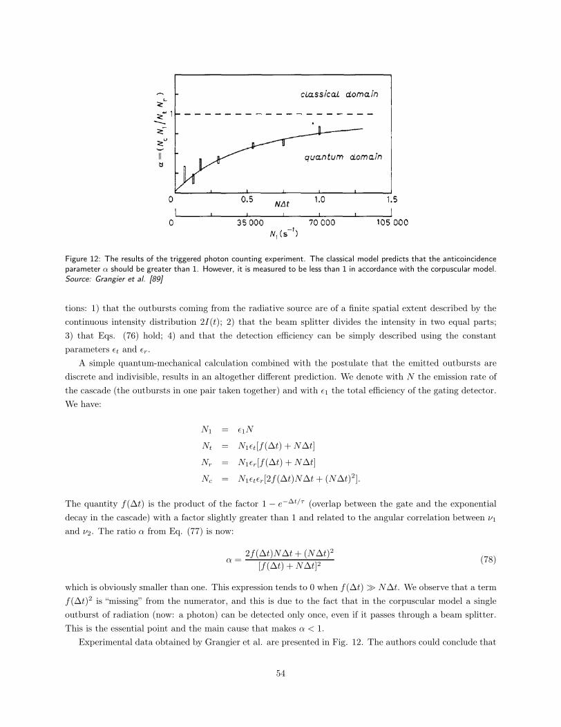
Figure 12: The results of the triggered photon counting experiment. The classical model predicts that the anticoincidenceparameter α should be greater than 1. However, it is measured to be less than 1 in accordance with the corpuscular model.Source: Grangier et al. [89]

tions: 1) that the outbursts coming from the radiative source are of a finite spatial extent described by the

continuous intensity distribution 2I(t); 2) that the beam splitter divides the intensity in two equal parts;

3) that Eqs. (76) hold; 4) and that the detection efficiency can be simply described using the constant

parameters ǫt and ǫr.

A simple quantum-mechanical calculation combined with the postulate that the emitted outbursts are

discrete and indivisible, results in an altogether different prediction. We denote with N the emission rate of

the cascade (the outbursts in one pair taken together) and with ǫ1 the total efficiency of the gating detector.

We have:

N1 = ǫ1N

Nt = N1ǫt[f(∆t) +N∆t]

Nr = N1ǫr[f(∆t) +N∆t]

Nc = N1ǫtǫr[2f(∆t)N∆t+ (N∆t)2].

The quantity f(∆t) is the product of the factor 1 − e−∆t/τ (overlap between the gate and the exponential

decay in the cascade) with a factor slightly greater than 1 and related to the angular correlation between ν1and ν2. The ratio α from Eq. (77) is now:

α =2f(∆t)N∆t+ (N∆t)2

[f(∆t) +N∆t]2(78)

which is obviously smaller than one. This expression tends to 0 when f(∆t) ≫ N∆t. We observe that a term

f(∆t)2 is “missing” from the numerator, and this is due to the fact that in the corpuscular model a single

outburst of radiation (now: a photon) can be detected only once, even if it passes through a beam splitter.

This is the essential point and the main cause that makes α < 1.

Experimental data obtained by Grangier et al. are presented in Fig. 12. The authors could conclude that

54

their anticoincidence measurements confirmed the corpuscular model; N∆t was varied and α was measured

to be indeed smaller than one and in accordance with Eq. (78). Their analysis and empirical results are

rather solid, but nonetheless there are several loopholes that should be pointed out.

Firstly, we can question the second assumption from the list above: Grangier et al. assumed that the

beam splitter either divides the intensity of a single radiation outburst in two equal parts (in the undulatory

model) or does not divide it at all (in the corpuscular model). If we now limit our attention to the undulatory

model, it is certainly true that the beam splitter works on the 50:50 principle, if the time scale involved is long

enough, i.e. if we integrate the intensity coming from the two outputs of the beam splitter over sufficiently

long time. The question remains whether the 50:50-manner of splitting up the incoming radiation occurs also

in the very low intensity regime. If not, then the derivation of Eq. (77) would be incorrect. Shortcomings

of the standard beam splitter models will be discussed in Section 5.2.3; we notice that a classical model

improved in this respect could account for the observation of α < 1.

Secondly, Panarella [71] pointed out that the quantum efficiency of the detectors used (which was not

explicitly stated) had to be limited, so out of N of the (postulated) photons impinging on the detector only a

minor fraction could lead to an emission of photoelectrons. The remaining photons went altogether unnoticed

by the apparatus, so any information about their arrangement in space (whether they were indeed isolated

in space, as the authors assumed, or rather grouped together). A model with “photon clumps”, also due to

Panarella, will be discussed in Chapter 9.1.

Thirdly, it should be noticed that the analysis due to Grangier et al. was done more carefully in the case

of the corpuscular model than in the case of the undulatory one, since only in the first one they consider the

overlap between the gate and the exponential decay and the angular correlation between ν1 and ν2.

Finally (but this argument is by no means least important) the experiment involved a nonclassical light

source. A similar anticoincidence effect would not be observed in the case of a classical light source like

laser, as we will see in Chapter 7.1, and differences between classical and nonclassical light sources in the

context of photocounting measurement will be discussed in Sect. 5.1.4. Thus we have to keep in mind that

the corpuscular behaviour exhibited in the anticoincidence experiment was demonstrated neither for thermal

light source nor for coherent light source.

55

56

4 Classical description of optical coherence and correlations

In the following two chapters we will present the theoretical background for our preliminary measurements in

Chapter 6 and experimental illustration of the wave-particle duality in Chapter 7. We begin by elaborating on

the concept of optical coherence and optical correlations, the inclusion of which is necessary in any discussion

of the interference phenomena. For this reason the term “coherence” had to be used already in Chapter

3.2 in our treatment of the Michelson interferometer, but there we have avoided definitions and detailed

considerations. This will be made up for in the present chapter which is based on Saleh and Teich [48]

(Chapter 11), Loudon [52] (Chapter 3) and Mandel and Wolf [55] (Chapters 2, 4 and 12).

The examination of optical coherence can be conducted both on the classical and the quantum-mechanical

grounds. We will use the first approach, but we will also mention the important result implied by the quantum

theory that is absent in the classical one (final paragraphs of Ch. 4.3). More emphasis is put on the classical

description, because it seems to be the most natural way of describing conditions under which interference

occurs. However, the quantum model seems to be indispensible in specific experimental situations where

so-called antibunching phenomena arise, and we will come back to this issue in Sect. 5.1.4, after we have

reviewed different photodetection models.

This chapters starts with the presentation of the complex analytic signal, a commonly used representation

of the optical field (Ch. 4.1). The concept of optical coherence is introduced in the next two sections, first

in a rather qualitative way (Ch. 4.2), and then rigorously, using the so-called coherence degrees (Ch. 4.3).

As illustrations we use results from a numerical simulation of the thermal emission of light. The theory of

optical coherence is then applied to interferometry experiments, and a simple formula describing the inter-

ference fringes emerges (Ch. 4.4).

4.1 The complex analytic signal

When working with optical fields it is desirable to find a convenient mathematical representation of the phys-

ically measurable signals. Since the electric field E and the magnetic field B are related through Maxwell’s

equations, in far-field approximations limiting our attention to only one of them, say E, is enough. Further-

more, to simplify the analysis, one frequently works with a single component of the electric field. Thus the

optical field is considered to be a scalar wavefield characterized by that component, and it can be represented

as the so-called complex analytic signal. A full vectorial treatment is also possible, but will be unnecessary

57

for us. We present the concept of the complex analytic signal in the scalar framework, and our description

is based on Chapter 3.1 of Mandel and Wolf [55], but some calculational details have been changed. The

formalism of the complex analytic signal as applied to vector wavefields is to be found in ibid., Chapter 6.

Assume that our real signal, x(t), is one of the components of the electric field. The real signal x(t) can

be expressed in terms of its Fourier transform x(ω):

x(t) =1√2π

∫ ∞

−∞x(ω)e−iωt dω (79)

where the Fourier transform (alternatively called the spectral amplitude) is given as:

x(ω) =1√2π

∫ ∞

−∞x(t)eiωt dt. (80)

The frequency variable ω, however, does not need to run from −∞ to +∞, because information about

x(ω < 0) is already contained in x(ω > 0) (or vice versa). This is due to the fact that x(t) is real, because

with x∗(t) = x(t) we have:

x(−ω) =1√2π

∫ ∞

−∞x(t)e−iωt dt =

1√2π

∫ ∞

−∞x∗(t)e−iωt dt = x∗(ω).

This motivates the introduction of a new function z(t) defined again as the Fourier integral. This function is

the complex analytic signal associated with x(t):

z(t) ≡ 1√2π

∫ ∞

−∞z(ω)e−iωt dω (81)

where:

z(ω) ≡

x(ω), ω ≥ 0

0, ω < 0,

so z(t) can be written as:

z(t) =1√2π

∫ ∞

0

x(ω)e−iωt dω. (82)

In other words we have to set to zero the negative frequencies in the Fourier expression for x(t), Eq. (79).

However, despite the formal similarity between x(t) and z(t), the latter is generally not real, because:

z∗(t) =1√2π

∫ ∞

0

x∗(ω)eiωt dω =1√2π

∫ ∞

0

x(−ω)eiωt dω =1√2π

∫ 0

−∞x(ω)e−iωt dω 6= z(t).

On the other hand this gives us a simple relation between x(t) and its complex analytic signal:

x(t) =1√2π

∫ ∞

−∞x(ω)e−iωt dω =

1√2π

(∫ 0

−∞+

∫ ∞

0

)

x(ω)e−iωt dω = z(t) + z∗(t) = 2ℜ[z(t)]. (83)

58

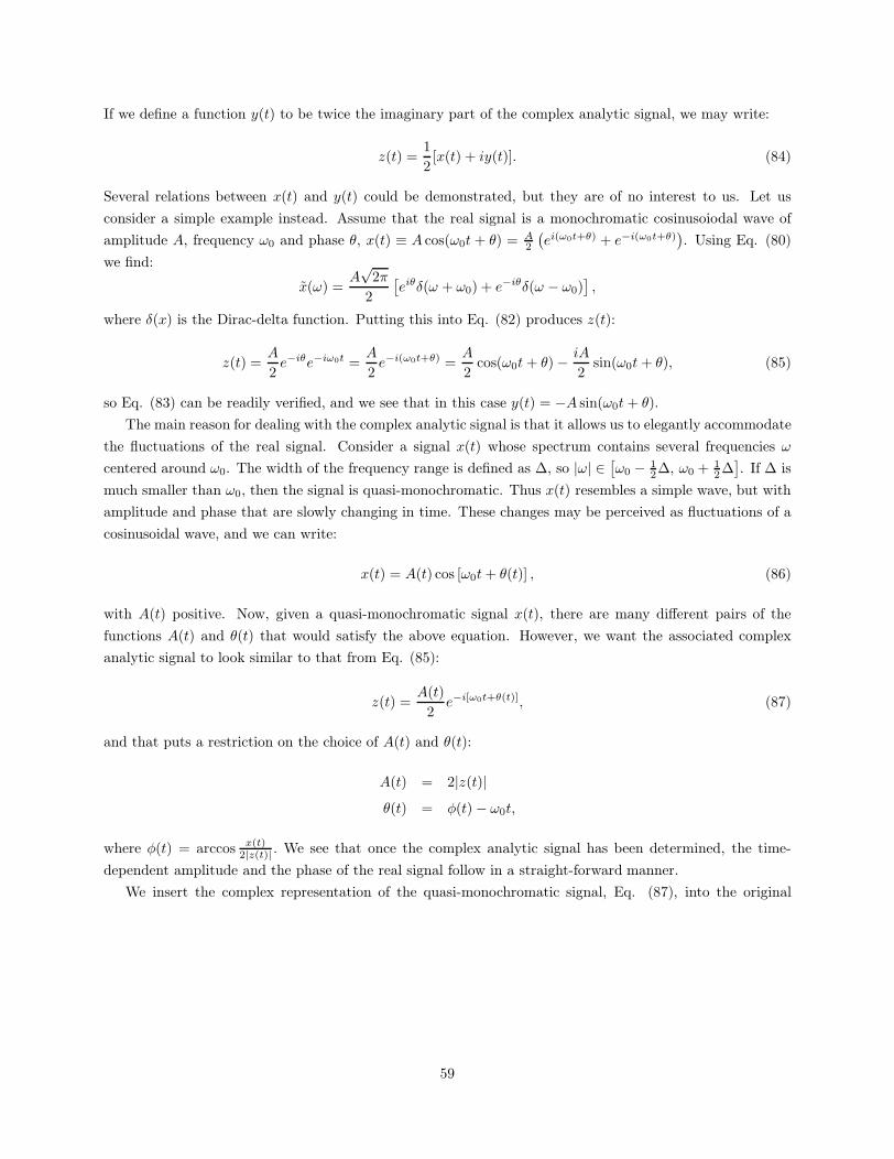
If we define a function y(t) to be twice the imaginary part of the complex analytic signal, we may write:

z(t) =1

2[x(t) + iy(t)]. (84)

Several relations between x(t) and y(t) could be demonstrated, but they are of no interest to us. Let us

consider a simple example instead. Assume that the real signal is a monochromatic cosinusoiodal wave of

amplitude A, frequency ω0 and phase θ, x(t) ≡ A cos(ω0t + θ) = A2

(

ei(ω0t+θ) + e−i(ω0t+θ))

. Using Eq. (80)

we find:

x(ω) =A√

2π

2

[

eiθδ(ω + ω0) + e−iθδ(ω − ω0)]

,

where δ(x) is the Dirac-delta function. Putting this into Eq. (82) produces z(t):

z(t) =A

2e−iθe−iω0t =

A

2e−i(ω0t+θ) =

A

2cos(ω0t+ θ) − iA

2sin(ω0t+ θ), (85)

so Eq. (83) can be readily verified, and we see that in this case y(t) = −A sin(ω0t+ θ).

The main reason for dealing with the complex analytic signal is that it allows us to elegantly accommodate

the fluctuations of the real signal. Consider a signal x(t) whose spectrum contains several frequencies ω

centered around ω0. The width of the frequency range is defined as ∆, so |ω| ∈[

ω0 − 12∆, ω0 + 1

2∆]

. If ∆ is

much smaller than ω0, then the signal is quasi-monochromatic. Thus x(t) resembles a simple wave, but with

amplitude and phase that are slowly changing in time. These changes may be perceived as fluctuations of a

cosinusoidal wave, and we can write:

x(t) = A(t) cos [ω0t+ θ(t)] , (86)

with A(t) positive. Now, given a quasi-monochromatic signal x(t), there are many different pairs of the

functions A(t) and θ(t) that would satisfy the above equation. However, we want the associated complex

analytic signal to look similar to that from Eq. (85):

z(t) =A(t)

2e−i[ω0t+θ(t)], (87)

and that puts a restriction on the choice of A(t) and θ(t):

A(t) = 2|z(t)|θ(t) = φ(t) − ω0t,

where φ(t) = arccos x(t)2|z(t)| . We see that once the complex analytic signal has been determined, the time-

dependent amplitude and the phase of the real signal follow in a straight-forward manner.

We insert the complex representation of the quasi-monochromatic signal, Eq. (87), into the original

59

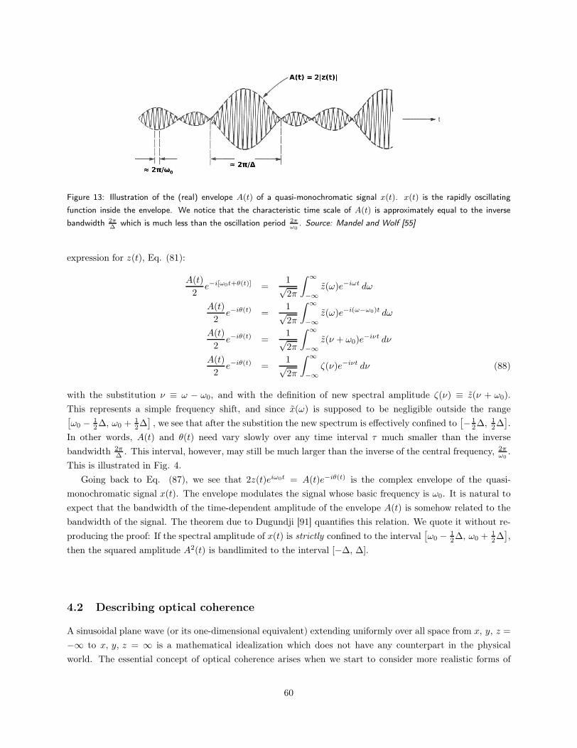
Figure 13: Illustration of the (real) envelope A(t) of a quasi-monochromatic signal x(t). x(t) is the rapidly oscillating

function inside the envelope. We notice that the characteristic time scale of A(t) is approximately equal to the inverse

bandwidth 2π∆

which is much less than the oscillation period 2πω0

. Source: Mandel and Wolf [55]

expression for z(t), Eq. (81):

A(t)

2e−i[ω0t+θ(t)] =

1√2π

∫ ∞

−∞z(ω)e−iωt dω

A(t)

2e−iθ(t) =

1√2π

∫ ∞

−∞z(ω)e−i(ω−ω0)t dω

A(t)

2e−iθ(t) =

1√2π

∫ ∞

−∞z(ν + ω0)e

−iνt dν

A(t)

2e−iθ(t) =

1√2π

∫ ∞

−∞ζ(ν)e−iνt dν (88)

with the substitution ν ≡ ω − ω0, and with the definition of new spectral amplitude ζ(ν) ≡ z(ν + ω0).

This represents a simple frequency shift, and since x(ω) is supposed to be negligible outside the range[

ω0 − 12∆, ω0 + 1

2∆]

, we see that after the substition the new spectrum is effectively confined to[

− 12∆, 1

2∆]

.

In other words, A(t) and θ(t) need vary slowly over any time interval τ much smaller than the inverse

bandwidth 2π∆ . This interval, however, may still be much larger than the inverse of the central frequency, 2π

ω0.

This is illustrated in Fig. 4.

Going back to Eq. (87), we see that 2z(t)eiω0t = A(t)e−iθ(t) is the complex envelope of the quasi-

monochromatic signal x(t). The envelope modulates the signal whose basic frequency is ω0. It is natural to

expect that the bandwidth of the time-dependent amplitude of the envelope A(t) is somehow related to the

bandwidth of the signal. The theorem due to Dugundji [91] quantifies this relation. We quote it without re-

producing the proof: If the spectral amplitude of x(t) is strictly confined to the interval[

ω0 − 12∆, ω0 + 1

2∆]

,

then the squared amplitude A2(t) is bandlimited to the interval [−∆, ∆].

4.2 Describing optical coherence

A sinusoidal plane wave (or its one-dimensional equivalent) extending uniformly over all space from x, y, z =

−∞ to x, y, z = ∞ is a mathematical idealization which does not have any counterpart in the physical

world. The essential concept of optical coherence arises when we start to consider more realistic forms of

60

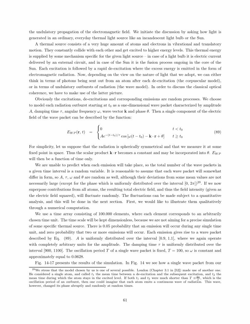
the undulatory propagation of the electromagnetic field. We initiate the discussion by asking how light is

generated in an ordinary, everyday thermal light source like an incandescent light bulb or the Sun.

A thermal source consists of a very huge amount of atoms and electrons in vibrational and translatory

motion. They constantly collide with each other and get excited to higher energy levels. This thermal energy

is supplied by some mechanism specific for the given light source – in case of a light bulb it is electric current

delivered by an external circuit, and in case of the Sun it is the fusion process ongoing in the core of the

Sun. Each excitation is followed by a rapid de-excitation where the excess energy is emitted in the form of

electromagnetic radiation. Now, depending on the view on the nature of light that we adopt, we can either

think in terms of photons being sent out from an atom after each de-excitation (the corpuscular model),

or in terms of undulatory outbursts of radiation (the wave model). In order to discuss the classical optical

coherence, we have to make use of the latter picture.

Obviously the excitations, de-excitations and corresponding emissions are random processes. We choose

to model each radiation outburst starting at t0 as a one-dimensional wave packet characterized by amplitude

A, damping time τ , angular frequency ω, wave vector k and phase θ. Then a single component of the electric

field of the wave packet can be described by the function:

EWP (r, t) =

0 t < t0

Ae−(t−t0)/τ cos [ω(t− t0) − k · r + θ] t ≥ t0(89)

For simplicity, let us suppose that the radiation is spherically symmetrical and that we measure it at some

fixed point in space. Thus the scalar product k · r becomes a constant and may be incorporated into θ. EWP

will then be a function of time only.

We are unable to predict when each emission will take place, so the total number of the wave packets in

a given time interval is a random variable. It is reasonable to assume that each wave packet will somewhat

differ in form, so A, τ , ω and θ are random as well, although their deviations from some mean values are not

necessarily large (except for the phase which is uniformly distributed over the interval [0, 2π])29. If we now

superpose contributions from all atoms, the resulting total electric field, and thus the field intensity (given as

the electric field squared), will fluctuate randomly. The fluctuations can be made subject to a quantitative

analysis, and this will be done in the next section. First, we would like to illustrate them qualitatively

through a numerical computation.

We use a time array consisting of 100.000 elements, where each element corresponds to an arbitrarily

chosen time unit. The time scale will be kept dimensionless, because we are not aiming for a precise simulation

of some specific thermal source. There is 0.05 probability that an emission will occur during any single time

unit, and zero probability that two or more emissions will occur. Each emission gives rise to a wave packet

described by Eq. (89). A is uniformly distributed over the interval [0.9, 1.1], where we again operate

with completely arbitrary units for the amplitude. The damping time τ is uniformly distributed over the

interval [900, 1100]. The oscillation period T of a single wave packet is fixed, T = 100, so ω is constant and

approximately equal to 0.0628.

Fig. 14-17 presents the results of the simulation. In Fig. 14 we see how a single wave packet from our

29We stress that the model chosen by us is one of several possible. Loudon (Chapter 3.1 in [52]) made use of another one.He considered a single atom, and called t1 the mean time between a de-excitation and the subsequent excitation, and t2 themean time during which the atom stays in the excited level. If both t1 and t2 were much shorter than T ≡ 2π

ω, which is the

oscillation period of an outburst, then one could imagine that each atom emits a continuous wave of radiation. This wave,however, changed its phase abruptly and randomly at random times.

61

34 34.5 35 35.5 36 36.5 37 37.5 380

0.2

0.4

0.6

0.8

1

1.2

Time [τ]

Inte

nsity

Figure 14: An intensity distribution of a single wave packet from our simulation. Such wave packet is assumed to representthe radiation outburst emitted by an atom due to its excitation and the subsequent de-excitation. The start amplitude, thephase and the damping time are chosen randomly for each packet, but all of them are of the same form as the one depictedin the figure. Notice that the time is given in the units of τ where τ is the damping time. The same time scale is employedin the next three figures.

model looks like. Fig. 15 shows the development of the intensity over the whole time interval (the so-called

time series). It is highly irregular, but it is also characterized by a presence of easily discernible “spikes”. In

Fig. 16 we zoom in a part of the previous figure. Now the rapid oscillations corresponding to the wave packet

frequency ω are visible. More importantly, we observe that during short time intervals (but still larger than

T ), the intensity develops in at least partially predictable way, rising and then declining again. One such

interval has been marked with a double arrow labelled as τc which stands for coherence time, and the name

has been chosen with the foresight of the further results.

Qualitatively speaking, the coherence time represents the time interval over which the evolution of an

electromagnetic wave is regular. Obviously a plane electromagnetic wave has infinite coherence time. On the

other hand, even a highly erratic radiation pattern, as the one modelled in Fig. 15-16, has a coherence time

that is small, but finite. The coherence time can be quantified in at least two different ways, and we will

examine the rigorous mathematical definitions in the next section.

Finally, Fig. 17 presents the same part of the plot as Fig. 16, but with the intensity cycle-averaged. In

this way we have removed the basic oscillatory pattern, but the plot is now less smooth. This is because the

time resolution in our simulation was not very large to begin with. Fig. 17 is included for the sake of graphical

completeness, since sometimes graphs like Fig. 15 or 16 are presented with the intensity cycle-averaged.

The discussion of the intensity fluctuations of a thermal source has allowed us to introduce the concept of

coherence time in a natural way. In fact, the same concept can be defined very simply on the phenomenological

grounds as well. Consider an interferometry experiment of the Michelson type as presented in Chapter 3.2.

Assume that the light source emits quasi-monochromatic radiation of bandwidth ∆f , and that the time delay

introduced between the two partial beams is equal to ∆t. Now, it is a well-known experimental fact (Mandel

62

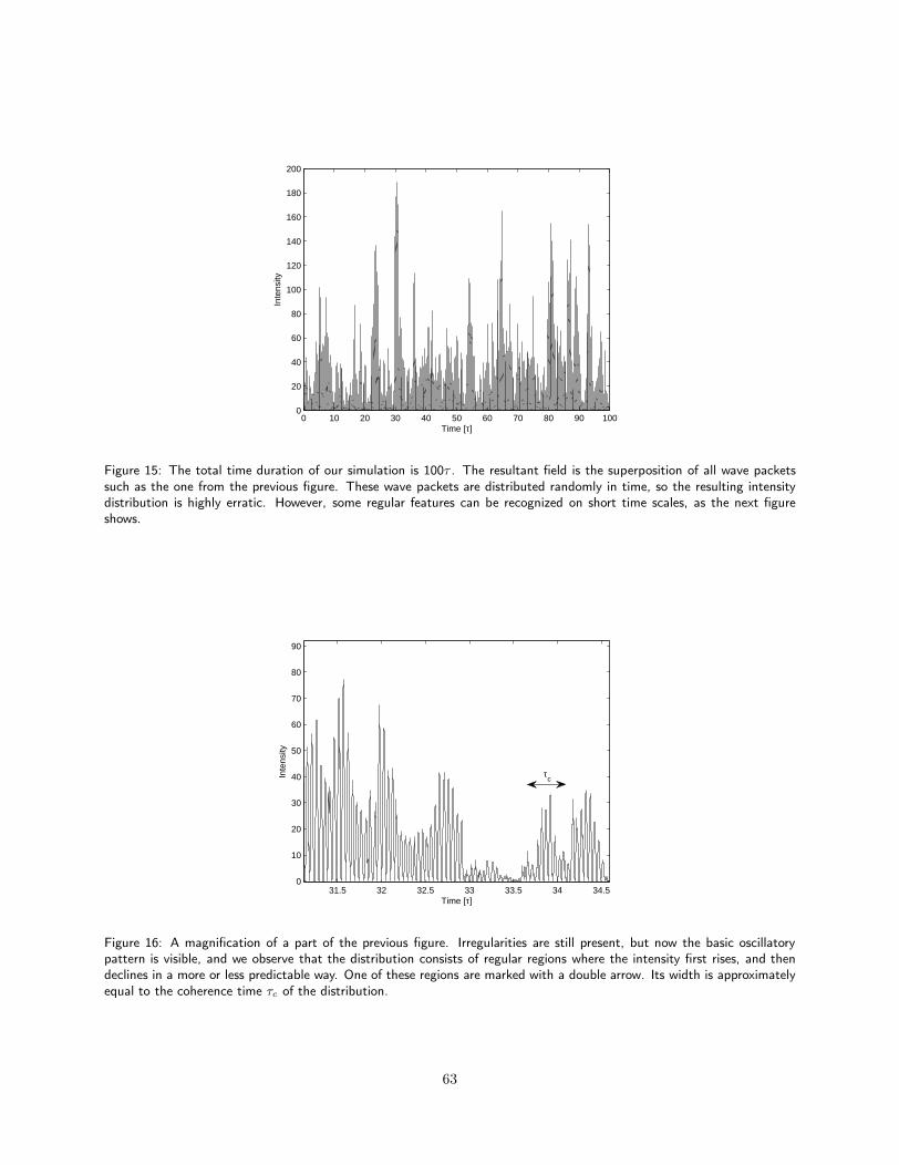
0 10 20 30 40 50 60 70 80 90 1000

20

40

60

80

100

120

140

160

180

200

Time [τ]

Inte

nsity

Figure 15: The total time duration of our simulation is 100τ . The resultant field is the superposition of all wave packetssuch as the one from the previous figure. These wave packets are distributed randomly in time, so the resulting intensitydistribution is highly erratic. However, some regular features can be recognized on short time scales, as the next figureshows.

31.5 32 32.5 33 33.5 34 34.50

10

20

30

40

50

60

70

80

90

Time [τ]

Inte

nsity

τc

Figure 16: A magnification of a part of the previous figure. Irregularities are still present, but now the basic oscillatorypattern is visible, and we observe that the distribution consists of regular regions where the intensity first rises, and thendeclines in a more or less predictable way. One of these regions are marked with a double arrow. Its width is approximatelyequal to the coherence time τc of the distribution.

63

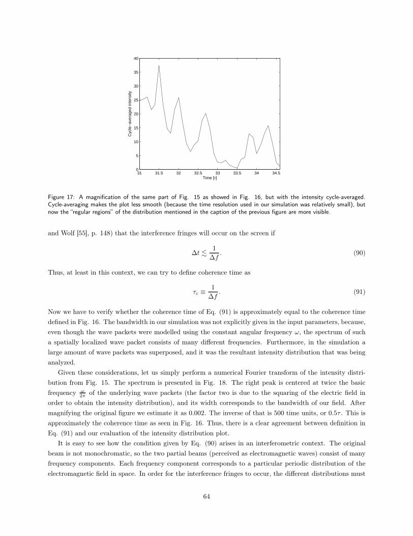
31 31.5 32 32.5 33 33.5 34 34.50

5

10

15

20

25

30

35

40

Time [τ]

Cyc

le−

aver

aged

inte

nsity

Figure 17: A magnification of the same part of Fig. 15 as showed in Fig. 16, but with the intensity cycle-averaged.Cycle-averaging makes the plot less smooth (because the time resolution used in our simulation was relatively small), butnow the “regular regions” of the distribution mentioned in the caption of the previous figure are more visible.

and Wolf [55], p. 148) that the interference fringes will occur on the screen if

∆t .1

∆f. (90)

Thus, at least in this context, we can try to define coherence time as

τc ≡ 1

∆f. (91)

Now we have to verify whether the coherence time of Eq. (91) is approximately equal to the coherence time

defined in Fig. 16. The bandwidth in our simulation was not explicitly given in the input parameters, because,

even though the wave packets were modelled using the constant angular frequency ω, the spectrum of such

a spatially localized wave packet consists of many different frequencies. Furthermore, in the simulation a

large amount of wave packets was superposed, and it was the resultant intensity distribution that was being

analyzed.

Given these considerations, let us simply perform a numerical Fourier transform of the intensity distri-

bution from Fig. 15. The spectrum is presented in Fig. 18. The right peak is centered at twice the basic

frequency ω2π of the underlying wave packets (the factor two is due to the squaring of the electric field in

order to obtain the intensity distribution), and its width corresponds to the bandwidth of our field. After

magnifying the original figure we estimate it as 0.002. The inverse of that is 500 time units, or 0.5τ . This is

approximately the coherence time as seen in Fig. 16. Thus, there is a clear agreement between definition in

Eq. (91) and our evaluation of the intensity distribution plot.

It is easy to see how the condition given by Eq. (90) arises in an interferometric context. The original

beam is not monochromatic, so the two partial beams (perceived as electromagnetic waves) consist of many

frequency components. Each frequency component corresponds to a particular periodic distribution of the

electromagnetic field in space. In order for the interference fringes to occur, the different distributions must

64

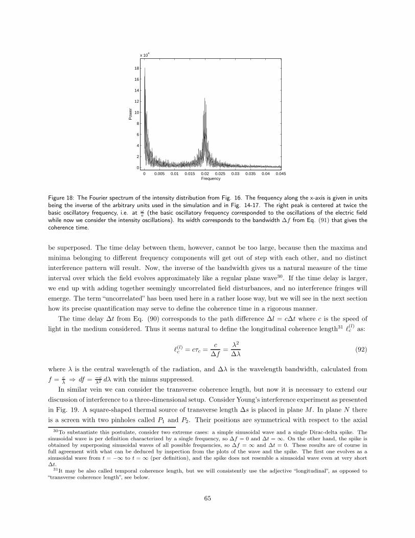
0 0.005 0.01 0.015 0.02 0.025 0.03 0.035 0.04 0.045

0

2

4

6

8

10

12

14

16

18

x 104

Frequency

Pow

er

Figure 18: The Fourier spectrum of the intensity distribution from Fig. 16. The frequency along the x-axis is given in unitsbeing the inverse of the arbitrary units used in the simulation and in Fig. 14-17. The right peak is centered at twice thebasic oscillatory frequency, i.e. at ω

π(the basic oscillatory frequency corresponded to the oscillations of the electric field

while now we consider the intensity oscillations). Its width corresponds to the bandwidth ∆f from Eq. (91) that gives thecoherence time.

be superposed. The time delay between them, however, cannot be too large, because then the maxima and

minima belonging to different frequency components will get out of step with each other, and no distinct

interference pattern will result. Now, the inverse of the bandwidth gives us a natural measure of the time

interval over which the field evolves approximately like a regular plane wave30. If the time delay is larger,

we end up with adding together seemingly uncorrelated field disturbances, and no interference fringes will

emerge. The term “uncorrelated” has been used here in a rather loose way, but we will see in the next section

how its precise quantification may serve to define the coherence time in a rigorous manner.

The time delay ∆t from Eq. (90) corresponds to the path difference ∆l = c∆t where c is the speed of

light in the medium considered. Thus it seems natural to define the longitudinal coherence length31 ℓ(l)c as:

ℓ(l)c = cτc =c

∆f=

λ2

∆λ(92)

where λ is the central wavelength of the radiation, and ∆λ is the wavelength bandwidth, calculated from

f = cλ ⇒ df = −c

λ2 dλ with the minus suppressed.

In similar vein we can consider the transverse coherence length, but now it is necessary to extend our

discussion of interference to a three-dimensional setup. Consider Young’s interference experiment as presented

in Fig. 19. A square-shaped thermal source of transverse length ∆s is placed in plane M . In plane N there

is a screen with two pinholes called P1 and P2. Their positions are symmetrical with respect to the axial

30To substantiate this postulate, consider two extreme cases: a simple sinusoidal wave and a single Dirac-delta spike. Thesinusoidal wave is per definition characterized by a single frequency, so ∆f = 0 and ∆t = ∞. On the other hand, the spike isobtained by superposing sinusoidal waves of all possible frequencies, so ∆f = ∞ and ∆t = 0. These results are of course infull agreement with what can be deduced by inspection from the plots of the wave and the spike. The first one evolves as asinusoidal wave from t = −∞ to t = ∞ (per definition), and the spike does not resemble a sinusoidal wave even at very short∆t.

31It may be also called temporal coherence length, but we will consistently use the adjective “longitudinal”, as opposed to“transverse coherence length”, see below.

65

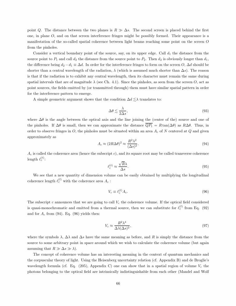
point Q. The distance between the two planes is R ≫ ∆s. The second screen is placed behind the first

one, in plane O, and on that screen interference fringes might be possibly formed. Their appearance is a

manifestation of the so-called spatial coherence between light beams reaching some point on the screen O

from the pinholes.

Consider a vertical boundary point of the source, say, on its upper edge. Call d1 the distance from the

source point to P1 and call d2 the distance from the source point to P2. Then d2 is obviously longer than d1,

the difference being d2−d1 ≡ ∆d. In order for the interference fringes to form on the screen O, ∆d should be

shorter than a central wavelength of the radiation, λ (which is assumed much shorter than ∆s). The reason

is that if the radiation is to exhibit any central wavelength, then its character must remain the same during

spatial intervals that are of magnitude λ (see Ch. 4.1). Since the pinholes, as seen from the screen O, act as

point sources, the fields emitted by (or transmitted through) them must have similar spatial pattern in order

for the interference pattern to emerge.

A simple geometric argument shows that the condition ∆d .λ translates to:

∆θ .λ

2∆s, (93)

where ∆θ is the angle between the optical axis and the line joining the (center of the) source and one of

the pinholes. If ∆θ is small, then we can approximate the distance QP1 = R tan(∆θ) as R∆θ. Thus, in

order to observe fringes in O, the pinholes must be situated within an area Ac of N centered at Q and given

approximately as

Ac ≈ (2R∆θ)2 ≈ R2λ2

(∆s)2. (94)

Ac is called the coherence area (hence the subscript c), and its square root may be called transverse coherence

length ℓ(t)c :

ℓ(t)c ≈√Rλ

∆s. (95)

We see that a new quantity of dimension volume can be easily obtained by multiplying the longitudinal

coherence length ℓ(l)c with the coherence area Ac :

Vc ≡ ℓ(l)c Ac. (96)

The subscript c announces that we are going to call Vc the coherence volume. If the optical field considered

is quasi-monochromatic and emitted from a thermal source, then we can substitute for ℓ(l)c from Eq. (92)

and for Ac from (94). Eq. (96) yields then:

Vc ≈ R2λ4

∆λ(∆s)2, (97)

where the symbols λ, ∆λ and ∆s have the same meaning as before, and R is simply the distance from the

source to some arbitrary point in space around which we wish to calculate the coherence volume (but again

assuming that R ≫ ∆s≫ λ).

The concept of coherence volume has an interesting meaning in the context of quantum mechanics and

the corpuscular theory of light. Using the Heisenberg uncertainty relation (cf. Appendix B) and de Broglie’s

wavelength formula (cf. Eq. (205), Appendix C) one can show that in a spatial region of volume Vc the

photons belonging to the optical field are intrinsically indistinguishable from each other (Mandel and Wolf

66

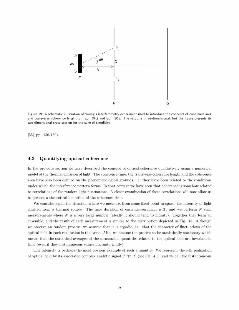
Figure 19: A schematic illustration of Young’s interferometry experiment used to introduce the concepts of coherence areaand transverse coherence length, cf. Eq. (94) and Eq. (95). The setup is three-dimensional, but the figure presents itstwo-dimensional cross-section for the sake of simplicity.

[55], pp. 156-159).

4.3 Quantifying optical coherence

In the previous section we have described the concept of optical coherence qualitatively using a numerical

model of the thermal emission of light. The coherence time, the transverse coherence length and the coherence

area have also been defined on the phenomenological grounds, i.e. they have been related to the conditions

under which the interference pattern forms. In that context we have seen that coherence is somehow related

to correlations of the random light fluctuations. A closer examination of these correlations will now allow us

to present a theoretical definition of the coherence time.

We consider again the situation where we measure, from some fixed point in space, the intensity of light

emitted from a thermal source. The time duration of each measurement is T , and we perform N such

measurements where N is a very large number (ideally it should tend to infinity). Together they form an

ensemble, and the result of each measurement is similar to the distribution depicted in Fig. 15. Although

we observe an random process, we assume that it is ergodic, i.e. that the character of fluctuations of the

optical field in each realization is the same. Also, we assume the process to be statistically stationary which

means that the statistical averages of the measurable quantities related to the optical field are invariant in

time (even if they instantaneous values fluctuate wildly).

The intensity is perhaps the most obvious example of such a quantity. We represent the i-th realization

of optical field by its associated complex analytic signal z(i)(r, t) (see Ch. 4.1), and we call the instantaneous

67

intensity of the i-th realization I(i)(r, t). The intensity averaged over the ensemble, I(r), is then given as:

I(r) =1

N

N∑

i=1

I(i)(r, t) =1

N

N∑

i=1

∣

∣

∣z(i)(r, t)

∣

∣

∣

2

≡ 〈|z(r, t)|2〉.

It is customary to use brackets 〈. . . 〉 to denote the ensemble average. The time variable disappears, because

due to the statistical stationarity the average will be time-independent per definition. However, when both

the ergodicity and stationarity assumptions hold, the averaging can be performed using a single realization

only. T must then be long enough, i.e. much longer than any characteristic time scale of the fluctuations

involved. Ideally it should tend to infinity, just as N above. Thus we have:

I(r) = 〈|z(r, t)|2〉 = limT→∞

1

T

∫ T/2

−T/2

|z(r, t)|2 dt.

The formal proof that under the described circumstances the ensemble average equals the time average can

be found, for instance, in Mandel and Wolf [55] (Sect. 2.2.2).

The characteristic time scale of the fluctuations involved in a random process is a central parameter

describing the process. We can quantify it by introducing a function which describes correlations between

two arbitrary temporal points of the optical field. This function, Γ(t1, t2), is called the autocorrelation

function, the two-time correlation function or the temporal coherence function. We will use the first name.

The autocorrelation is defined as:

Γ(t1, t2) ≡ 〈z∗(t1)z(t2)〉

Both Γ and z depend implicitly on the position in space, but since we assume that all measurements are

performed in the same spatial point, the variable r has now been omitted. Furthermore, since the processes

considered are statistically stationary, the autocorrelation function depends on its time arguments only

through the difference between them. Thus we can express it as:

Γ(∆t) = 〈z∗(t)z(t+ ∆t)〉 , (98)

where ∆t is the time delay and t can be chosen arbitrarily. We notice that the autocorrelation function is a

kind of “generalized intensity”, because for ∆t = 0 it yields:

Γ(0) = 〈z∗(t)z(t)〉 = I

It is customary to use the intensity in order to normalize the autocorrelation function so its absolute value

will be bounded by 0 and 1. Therefore we define the complex first-order degree of temporal coherence, γ(∆t),

as:

γ(∆t) ≡ Γ(∆t)

Γ(0)=

〈z∗(t)z(t+ ∆t)〉I

=〈z∗(t)z(t+ ∆t)〉

〈z∗(t)z(t)〉 , (99)

and it can be shown (Mandel and Wolf [55], Section 4.3.1) that with this definition 0 ≤ |γ(∆t)| ≤ 1. By

inspection, we see also that γ(0) = 1, so any temporal point is maximally correlated with itself which makes

good sense. Finally, the first order degree of temporal coherence is symmetric in ∆t, because γ(∆t) =

68

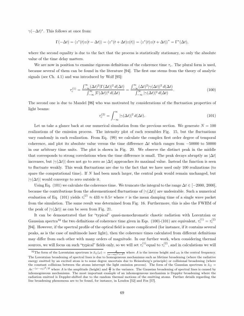
γ(−∆t)∗. This follows at once from:

Γ(−∆t) = 〈z∗(t)z(t− ∆t)〉 = 〈z∗(t+ ∆t)z(t)〉 = 〈z∗(t)z(t+ ∆t)〉∗ = Γ∗(∆t),

where the second equality is due to the fact that the process is statistically stationary, so only the absolute

value of the time delay matters.

We are now in position to examine rigorous definitions of the coherence time τc. The plural form is used,

because several of them can be found in the literature [94]. The first one stems from the theory of analytic

signals (see Ch. 4.1) and was introduced by Wolf [95]:

τ (1)c =

∫∞−∞(∆t)2|Γ(∆t)|2 d(∆t)∫∞−∞ |Γ(∆t)|2 d(∆t)

=

∫∞−∞(∆t)2|γ(∆t)|2 d(∆t)∫∞−∞ |γ(∆t)|2 d(∆t)

. (100)

The second one is due to Mandel [96] who was motivated by considerations of the fluctuation properties of

light beams:

τ (2)c =

∫ ∞

−∞|γ(∆t)|2 d(∆t). (101)

Let us take a glance back at our numerical simulation from the previous section. We generate N = 100

realizations of the emission process. The intensity plot of each resembles Fig. 15, but the fluctuations

vary randomly in each realization. From Eq. (99) we calculate the complex first order degree of temporal

coherence, and plot its absolute value versus the time difference ∆t which ranges from −50000 to 50000

in our arbitrary time units. The plot is shown in Fig. 20. We observe the distinct peak in the middle

that corresponds to strong correlations when the time difference is small. The peak decays abruptly as |∆t|increases, but |γ(∆t)| does not go to zero as |∆t| approaches its maximal value. Instead the function is seen

to fluctuate weakly. This weak fluctuations are due to the fact that we have used only 100 realizations (to

spare the computational time). If N had been much larger, the central peak would remain unchanged, but

|γ(∆t)| would converge to zero outside it.

Using Eq. (101) we calculate the coherence time. We truncate the integral to the range ∆t ∈ [−2000, 2000],

because the contributions from the aforementioned fluctuations of |γ(∆t)| are undesirable. Such a numerical

evaluation of Eq. (101) yields τ (2)c ≈ 433 ≈ 0.5τ where τ is the mean damping time of a single wave packet

from the simulation. The same result was determined from Fig. 16. Furthermore, this is also the FWHM of

the peak of |γ(∆t)| as can be seen from Fig. 21.

It can be demonstrated that for “typical” quasi-monochromatic chaotic radiation with Lorentzian or

Gaussian spectra32 the two definitions of coherence time given in Eqs. (100)-(101) are equivalent, τ (1)c = τ

(2)c

[94]. However, if the spectral profile of the optical field is more complicated (for instance, if it contains several

peaks, as is the case of multimode laser light), then the coherence times calculated from different definitions

may differ from each other with many orders of magnitude. In our further work, when considering thermal

sources, we will focus on such “typical” fields only, so we will set τ (1)c equal to τ (2)

c , and in calculations we will

32The form of the Lorentzian spectrum is xL(ω) = A(ω−ω0)2+A2 where A is the inverse height and ω0 is the central frequency.

The Lorentzian broadening of spectral lines is due to homogeneous mechanisms such as lifetime broadening (where the radiativeenergy emitted by an excited atom is to some degree uncertain due to Heisenberg’s principle) or collisional broadening (wherethe constant collisions between the atoms interrupt the light emission process). The form of the Gaussian spectrum is xG =

Ae−(ω−ω0)2/B where A is the amplitude (height) and B2

is the variance. The Gaussian broadening of spectral lines is caused byinhomogeneous mechanisms. The most important example of an inhomogeneous mechanism is Doppler broadening where theradiation emitted is Doppler-shifted due to the random thermal motions of the emitting atoms. Further details regarding theline broadening phenomena are to be found, for instance, in Loudon [52] and Fox [57].

69

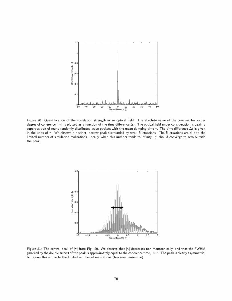
−50 −40 −30 −20 −10 0 10 20 30 40 500

0.2

0.4

0.6

0.8

1

1.2

Time difference [τ]

Cor

elat

ion

stre

ngth

, |γ|

Figure 20: Quantification of the correlation strength in an optical field. The absolute value of the complex first-orderdegree of coherence, |γ|, is plotted as a function of the time difference ∆t. The optical field under consideration is again asuperposition of many randomly distributed wave packets with the mean damping time τ . The time difference ∆t is givenin the units of τ . We observe a distinct, narrow peak surrounded by weak fluctuations. The fluctuations are due to thelimited number of simulation realizations. Ideally, when this number tends to infinity, |γ| should converge to zero outsidethe peak.

−2 −1.5 −1 −0.5 0 0.5 1 1.5 20

0.2

0.4

0.6

0.8

1

1.2

Time difference [τ]

Cor

elat

ion

stre

ngth

, |γ|

Figure 21: The central peak of |γ| from Fig. 20. We observe that |γ| decreases non-monotonically, and that the FWHM(marked by the double arrow) of the peak is approximately equal to the coherence time, 0.5τ . The peak is clearly asymmetric,but again this is due to the limited number of realizations (too small ensemble).

70

use Eq. (101).

We can now quantify the relation between the coherence time and the spectral width. We have seen that

the spectral profile z(ω) is given as the Fourier transform of the signal:

z(ω) =1√2π

∫ ∞

−∞z(t)e−iωt dt

Since each realization is of finite length T , the Fourier transform must in fact be first truncated:

zT (ω) =1√2π

∫ T/2

−T/2

z(t)e−iωt dt,

and then we can consider the limit as T → ∞. Taking the absolute value squared, ensemble averaging and

dividing by T yields a new quantity S(ω):

S(ω) = limT→∞

1

T

⟨

|zT (ω)|2⟩

.

This is the power spectral density, and S(ω) dω represents the average power per unit area per unit (angular)

frequency [48]. One can show that S(ω) is the Fourier transform of the autocorrelation function Γ(∆t):

S(ω) =1√2π

∫ ∞

−∞Γ(∆t)e−iω(∆t) d(∆t).

Furthermore, the total average intensity is given as the integral of S(ω):

I =

∫ ∞

0

S(ω) dω.

The spectral width ∆ω can be determined from the power spectral density. Again there are two different

definitions, each of which corresponds to one of the definitions of the coherence time τc from Eqs. (100) and

(101). The first one is:

∆ω(1) =

∫∞0

(ω − ω)2S2(ω) dω∫∞0 S2(ω) dω

,

with

ω =

∫∞0ωS2(ω) dω

∫∞0 S2(ω) dω

.

The second one is:

∆ω(2) =

(∫∞0S(ω) dω

)2

∫∞0 S2(ω) dω

.

These two spectral widths are related to the two coherence times in the following ways [94]:

τ (1)c ≥ 1

2∆ω(1)

τ (2)c =

2π

∆ω(2).

In particular we observe that the second pair of definitions reproduces the experimentally grounded coherence

time formula given by Eq. (91) (remember that ∆ω = 2π∆f). However, in both cases the coherence time is

71

not allowed to be shorter than approximately the inverse of the spectral width.

Up till now the position variable r has been suppressed in our treatment, i.e. we have assumed that all

measurements of the optical field are performed in the same point of space. This has allowed us to quantitively

examine the temporal coherence. Let us now generalize the formalism to two spatial points r1 and r2. We

introduce the cross-correlation function (also called the mutual coherence function):

Γ (r1, r2, ∆t) = 〈z∗ (r1, t) z (r2, t+ ∆t)〉, (102)

and the complex first-order degree of mutual coherence:

γ(r1, r2, ∆t) =Γ (r1, r2, ∆t)

√

Γ (r1, r1, 0)√

Γ (r2, r2, 0)=

Γ (r1, r2, ∆t)√

I(r1)I(r2), (103)

where we normalize the cross-correlation function with the help of the average intensities at the two spatial

points. Notice that we have called these two functions by the same Greek letters as the ones used before, Γ

and γ, in order to emphasize that the quantities from Eqs. (98)-(99) follow directly from the above expressions

(when r1 = r2). The absolute value of γ is still bounded between zero and unity, and, loosely speaking, the

larger it is, the stronger are the correlations of the optical field in two spacetime points.

Consider now again an extended thermal source of dimension ∆s lying in the origin O, and a point P

(in position r1) in space lying at distance R ≫ ∆s from the source. If we wish to determine the coherence

area around the point P , we can calculate the complex first-order degree of mutual coherence at different

points around P . Let us call one of these points Q (in position r2). If the distance difference∣

∣OQ−OP∣

∣ is

much smaller than the longitudinal coherence length ℓ(l)c = cτc, so that the optical field in P and Q is almost

completely temporally coherent, then we are effectively calculating γ(r1, r2, ∆t ≈ 0). For r1 = r2 the degree

of mutual coherence is 1. When |r2 − r1| increases, γ(r1, r2, ∆t ≈ 0) will decrease. As long as its value stays

relatively high (i.e. larger than some prescribed value), we say that the two points P and Q are partially

coherent in the spatial sense., and that Q is within coherence area relatively to P .

We will now introduce the concept of the complex second-order degree of coherence. It is obvious that

γ(r1, r2, ∆t) from Eq. (103) quantifies the correlations between field components in two different points

of the optical field. However, in many scenarios (the most notable being Hanbury Brown-Twiss interfer-

ometry experiment [97] [98]) it is desirable to examine the correlations between the intensities. A proper

generalization of γ is readily obtained:

γ(2)(r1, r2, ∆t) ≡ 〈ξ(r1, t)ξ(r2, t+ ∆t)〉I(r1)I(r2)

,

with ξ(r, t) = |z(r, t)|2 which is the instantaneous intensity. This is the definition of the second-order degree

of coherence. Using Cauchy’s inequality one can show (Loudon [52], Chapter 3.7) that

∞ ≥ γ(2)(r, r, ∆t) ≥ 1, ∆t = 0 (104)

∞ ≥ γ(2)(r, r, ∆t) ≥ 0, ∆t 6= 0.

These general inequalities are to be compared with γ(r, r, 0) = 1 and 1 ≥ |γ(r, r, ∆t)| ≥ 0 in the case of

the complex first-order degree of coherence which we will henceforth call γ(1). Even though the second-order

72

degree of coherence has no upper bound, it can be shown that

γ(2)(r, r, 0) ≥ γ(2)(r, r, ∆t). (105)

For the particular case of a quasi-monochromatic chaotic radiation these two coherence degrees are related:

γ(2)(r, r, ∆t) = 1 +∣

∣

∣γ(1)(r, r, ∆t)

∣

∣

∣

2

,

and the limiting values of the second-order degree of coherence are thus:

γ(2)(r, r, 0) = 2

γ(2)(r, r, |∆t| → ∞) → 1.

In the foregoing discussion of the second-order degree of coherence we have set r1 = r2 ≡ r. If we

now consider again two distinct spatial points r1 6= r2, we say that the optical field at these two points is

second-order coherent with time delay ∆t if∣

∣γ(1)(r1, r2, ∆t)∣

∣ = 1 and γ(2)(r1, r2, ∆t) = 1 are both satisfied.

Therefore the chaotic light will not be second-order coherent no matter what spatial points of the field are

being examined.

Finally we would like to mention an important result stemming from the theory of quantum correlations

which aims at describing and quantizing correlations of the quantized electromagnetic fields. This theory

represents electromagnetic fields as statistical mixtures of coherent states (see Ch. 2.4) using general dis-

tribution functions (which often cannot be reduced to ordinary probability distributions). It was developed

mainly by Glauber [43]. The presentation of his model in a satisfactory manner would be rather lengthy and

technical. Therefore for a full treatment we simply refer to Mandel and Wolf [55] (Chapter 12) or Loudon

[99], and here we quote only the result concerning the second-order degree of coherence which is of central

importance in our context. Namely, the theory of quantum correlations allows for a situation with:

γ(2)(r, r, 0) < 1 (106)

γ(2)(r, r, 0) < γ(2)(r, r, ∆t 6= 0) (107)

In other words, if the electromagnetic fields are quantized, then correlations of their fluctuations may be

weaker than the classical description predicts. These weak correlations correspond then to a high degree of

regularity in the stream of photons. For this reason light with γ(2)(r, r, 0) < γ(2)(r, r, ∆t 6= 0) (for some

∆t 6= 0, not necessarily for all ∆t) is called antibunched, while light with γ(2)(r, r, 0) > γ(2)(r, r, ∆t 6= 0)

is called bunched. Thus a situation with γ(2)(r, r, 0) > γ(2)(r, r, ∆t 6= 0) is admissible both in the classical

and in the quantum description of correlations. In the first case we explain it as a presence of high-intensity

fluctuations, in the second case as a presence of bunches of photons. The classical description, however,

cannot account for γ(2)(r, r, 0) < γ(2)(r, r, ∆t 6= 0).

We will discuss experimental demonstrations of photon antibunching in Sect. 5.1.4 in the context of differ-

ent photodetection models. There we will also comment on the link between photon bunching/antibunching

and photocount statistics.

73

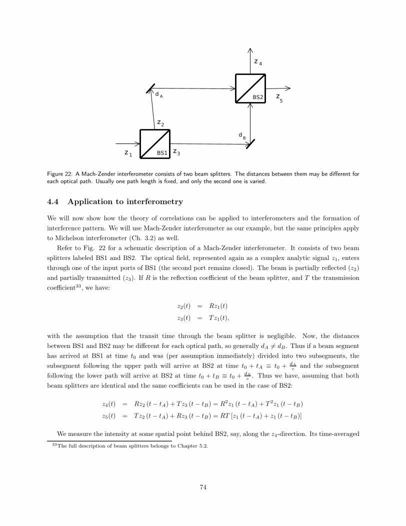
Figure 22: A Mach-Zender interferometer consists of two beam splitters. The distances between them may be different foreach optical path. Usually one path length is fixed, and only the second one is varied.

4.4 Application to interferometry

We will now show how the theory of correlations can be applied to interferometers and the formation of

interference pattern. We will use Mach-Zender interferometer as our example, but the same principles apply

to Michelson interferometer (Ch. 3.2) as well.

Refer to Fig. 22 for a schematic description of a Mach-Zender interferometer. It consists of two beam

splitters labeled BS1 and BS2. The optical field, represented again as a complex analytic signal z1, enters

through one of the input ports of BS1 (the second port remains closed). The beam is partially reflected (z2)

and partially transmitted (z3). If R is the reflection coefficient of the beam splitter, and T the transmission

coefficient33, we have:

z2(t) = Rz1(t)

z3(t) = Tz1(t),

with the assumption that the transit time through the beam splitter is negligible. Now, the distances

between BS1 and BS2 may be different for each optical path, so generally dA 6= dB . Thus if a beam segment

has arrived at BS1 at time t0 and was (per assumption immediately) divided into two subsegments, the

subsegment following the upper path will arrive at BS2 at time t0 + tA ≡ t0 + dA

c and the subsegment

following the lower path will arrive at BS2 at time t0 + tB ≡ t0 + dB

c . Thus we have, assuming that both

beam splitters are identical and the same coefficients can be used in the case of BS2:

z4(t) = Rz2 (t− tA) + Tz3 (t− tB) = R2z1 (t− tA) + T 2z1 (t− tB)

z5(t) = Tz2 (t− tA) +Rz3 (t− tB) = RT [z1 (t− tA) + z1 (t− tB)]

We measure the intensity at some spatial point behind BS2, say, along the z4-direction. Its time-averaged

33The full description of beam splitters belongs to Chapter 5.2.

74

value34 is:

Iout =⟨

|z4(t)|2⟩

=

|R|2|T |2⟨

|z1 (t− tA)|2 + |z1 (t− tB)|2 + z∗1 (t− tA) z1 (t− tB) + z1 (t− tA) z∗1 (t− tB)⟩

.(108)

Due to the statistical stationarity of the process, each of the two first terms in the brackets give the average

intensity Iin of the input beam:

⟨

|z1 (t− tA)|2⟩

=⟨

|z1 (t− tB)|2⟩

= Iin. (109)

The two last terms, however, can be rewritten and expressed with the help of the complex first-order degree

of coherence:

〈z∗1 (t− tA) z1 (t− tB) + z1 (t− tA) z∗1 (t− tB)〉 = 2ℜ [〈z∗1 (t− tA) z1 (t− tB)〉] = 2ℜ [〈z∗1(t)z1(t+ ∆t)〉] ,

with ∆t ≡ tA − tB = dA−dB

c and where the last equality is justified again by the statistical stationarity. We

continue:

2ℜ [〈z∗1(t)z1(t+ ∆t)〉] = 2ℜ[Γ(∆t)] = 2Iinℜ[

γ(1)(∆t)]

, (110)

with the help of Eqs. (98), (99) and (109). Putting back Eqs. (109)-(110) into Eq. (108) we obtain a simple

expression for the time-averaged output intensity:

Iout = 2Iin|R|2|T |2(

1 + ℜ[

γ(1)(∆t)])

(111)

We see that the output intensity of the Mach-Zender interferometer is related in a rather simple way to the

(real part of the) complex first-order degree of coherence. In the total absence of first-order correlations,

i.e. when γ(1)(∆t) = 0, the output intensity is constant and equal to 2Iin|R|2|T |2. However, the interference

fringes35 will occur when γ(1)(∆t) 6= 0, because then ℜ[

γ(1)(∆t)]

can be positive or negative. We conclude

that the formation of the fringes is dependent on the correlations in the input beam; or, equivalently, by

varying ∆t and measuring the output intensity, we can deduce the form of ℜ[

γ(1)(∆t)]

.

The above analysis of the Mach-Zender interferometry is applicable for both chaotic radiation from a

thermal source, for partially coherent light beam with coherence time long compared to the time needed for

the light to pass through the apparatus, and for perfectly coherent, idealized light beam with infinitely long

coherence time. In the first case, when |∆t| increases,∣

∣γ(1)∣

∣ will tend to zero, and the interference fringes

will be less and less visible, until at last Iout achieves the constant value of 2Iin|R|2|T |2. In the second case∣

∣γ(1)∣

∣ will also diminish with increasing |∆t|, but less rapidly. In the third case, one can show (Loudon [52],

Chapter 3.4) that γ(∆t) = e−iω∆t where ω is the angular frequency of the monochromatic light. Eq. (111)

34 We are using brackets, because we assume again that the emission process is ergodic, so the ensemble average equals the

time average.

35The term “interference fringes” is used here in a different way than in Chapter 3.2 where we discussed the Michelsoninterferometer. Now we are not talking about any spatial interference pattern, because the spatial variable r has been suppressedin our treatment of the Mach-Zender interferometer (as it is usually done). What we now mean with “fringes” is that when∆d ≡ dA − dB (and thus ∆t) is varied, the output intensity Iout measured at a single spatial point will get larger or smalleraccording to whether ℜ

ˆ

γ(1)(∆t)˜

increases or decreases.

75

implies that then Iout will oscillate in a sinusoidal fashion between 0 and 4Iin|R|2|T |2.In practice the above theory can be used to estimate coherence time τc (or, equivalently, longitudinal

coherence length ℓ(l)c ) of a light beam. One sends the beam through an interferometer and varies36 the path

length difference ∆d = c∆t between the two partial beams. The partial beams are recombined and the

visibility of interference fringes measured as a function of ∆d. As long as visibility remains high, ∆d must be

much less than ℓ(l)c . When ∆d tends to ℓ(l)c the visibility will decrease, and when the path length difference

exceeds the longitudinal coherence length, the interference pattern will no longer form, because then the

fluctuations in the two partial beams will be uncorrelated. This principle will be used in Chapter 6.2 where

we will measure the coherence length of our laser beam.

36For geometrical reasons it is more easily done with Michelson interferometer than Mach-Zender interferometer.

76

5 The main elements of the experimental setup: theoretical review

The following two chapters are dedicated to the three main elements of the experimental setup from Chapter

7 – the photodetector, the beam splitter and the laser beam. In this chapter we review the theoretical

background, and in the next chapter we state specifications of the elements and conduct some preliminary

measurements. Since the setup is being prepared from scratch, and since most of the components have not

been used before, such measurements are necessary. It seems only natural that their presentation is coupled

together with a review of the theoretical background. Hovewer, investigation of this background will give us

further insight into the wave-particle duality problem, because we will make use of different physical models

which assume that light is either an undulatory or a corpuscular phenomenon, and because we will discuss

how they differ and what their shortcomings are.

In Chapter 5.1 we are going to speak qualitatively about several different photodetection schemes (Sect.

5.1.1), and then discuss the photocount statistics in the framework of the semiclassical (Sect. 5.1.2) and the

corpuscular (Sect. 5.1.3) model. Concluding remarks regarding the two models are given in Sect. 5.1.4.

In Chapter 5.2 we present two theoretical models describing the beam splitter. The presentation will be

first done in a textbook manner (Sect 5.2.1-5.2.2), but then we will discuss the shortcomings of both models

(Sect. 5.2.3).

In Chapter 5.3 we will investigate the shape of the laser beam, since discussion of the beam shape is

necessary to properly set up optical elements in any laser experiment. That chapter is rather technical and

consists mainly of derivations – the central results, important for our further work in Chapter 6.1, are Eqs.

(158)-(165). The question of how the laser beam is actually generated has been left out. Although this

subject without a doubt is of relevance, its complexity makes the author unable to cover it in the thesis as

well. We can only refer to, for instance, Saleh and Teich [48], Milonni and Eberly [100] or Siegman [101].

In the following chapter both views on the nature of light will be used: the undulatory model (e.g.

when classically describing the beam splitter), and the corpuscular models (e.g. when reviewing the fully

quantum-mechanical theory of photocount statistics). Our treatment will therefore again exhibit the problem

of wave-particle duality, but the conceptual conflict between these different approaches will not be empha-

sized in this chapter. Let us keep in mind, however, that it may serve as a fine illustration of the duality (in

addition to the different considerations discussed in Chapter 3).

77

5.1 Photodetector

Consider a photon-counting experiment where we measure the incoming light beam with a single-photon

detector. The working of such a device is based on the (external or internal) photoelectric effect (for a

description of internal photoelectric effect see Ch. 3.3). As long as the intensity is not too high and we avoid

saturation, the response of the detector will consist of a series of discrete signals called photocounts. In the

following section we will develop basic statistical models that describe the distribution of the signals in time

and relate it to the type and intensity of the input radiation. We shall present two main approaches: the

semiclassical theory (Sect. 5.1.2) and the fully quantized model (Sect. 5.1.2). In our presentation we will

focus on the fundamental difference between the two models: That the latter is able to predict arbitrarily

small variance of the photocount number, while the semiclassical model sets a lower bound for it. We begin,

however, by reviewing different types of photodetectors (Sect. 5.1.1). The description is kept rather short

and qualitative, because the detailed examination would require us to review elements of solid-state and

semiconductor physics which are outside the scope of this thesis.

5.1.1 Types of photodetectors

A photodetector measures the intensity of electromagnetic radiation by converting its energy into a mea-

surable form. Photodetecting devices fall into two broad classes: photoelectric detectors that convert the

intensity into an electric current, and thermal detectors that convert the intensity into heat. The working

of the photoelectric detectors is based on the photoelectric effect which was explored in detail in Chapter

3.3. In that section we focused on the external photoelectric effect where electrons leave the photoelectric

material under an influence of electromagnetic radiation. In the case of the internal photoelectric effect the

excited electrons remain inside the photoelectric material, but increase its conductivity in a measurable way.

A typical example of a photodetector based on the external photoelectric effect is a photomultiplier tube

(also called a photomultiplier). When light impinges on the photocathode, the photoelectrons are emitted

and travel to the anode maintained at a higher electric potential. However, between the photocathode and the

anode there are several dynodes which amplify the electron current by the means of the secondary emission –

a phenomenon where a material emits additional electrons when impacted by an electron (or other material

particle) with sufficient energy. The amplified photoelectric current (the total amplification can be as high

as 108 [48]) is then measured, and related to the intensity of the incoming light.

In recent times, due to the progress in the fabrication of semiconductors, photodetectors based on the

internal photoelectric effect have gained popularity. For such devices the electromagnetic radiation transfers

its energy to an electron bound in the photosensitive part of the detector. The energy is not sufficient to eject

the electron from the material, but large enough to excite and move it from the lower energy level, called the

valence band, to the upper energy level, called the conduction band (thus the energy has to be greater than

the energy difference between the bands, called the band gap). Furthermore, the electron leaves behind it,

in the valence band, an excess of positive charge, called hole. The application of external electric field to the

material transports the excited electrons (and the holes) through it, thus producing a measurable electric

current. The electrons and the holes are collectively called carriers.

Similarly as in the case of photomultipliers, the internal photoelectric effect can be amplified by introducing

78

a gain mechanism into the structure of the semiconductor. This is what happens in the avalanche photodiodes

(APD) where the electric field is strong enough for a carrier to excite a new pair of carriers through the impact

ionization. In the process of impact ionization the original carrier has enough kinetic energy to promote a

bound electron to a state in the conduction band, thus creating a new electron-hole pair. The process is

repeated many times, so even low light intensity at the input would produce a relatively strong electrical

signal at the output. One could believe that increasing the strength of the external electric field would just

lead to a larger gain. However, several side-effects must be considered. The amplification is time consuming,

so large gain reduces the bandwidth of the detector. Furthermore, the process of amplification is inherently

random, so large gain will correspond to large noise. Finally, if the external electric field is too strong, there

will be spontaneous breakdowns, i.e. situations where the generation of the first carrier pair occurs because

of the field and not as the result of the impinging radiation.

If the (avalanche-amplified) electric signal caused by a single photocount is quickly quenched, but nonethe-

less registered on the output, then we are able to separate the signals corresponding to different photocounts.

Thus the response of the detector will be binarized – a single photocount will correspond to a short and

isolated output signal. With proper auxilliary electronic circuits in the detector module a high temporal

resolution (less than 1 ns) can be achieved, and the problem of noise reduced. However, there are several

drawbacks of such detection scheme. The detector will saturate much more easily, so the measured count

rate cannot be very high. The photocount statistics will be somewhat biased by the presence of dark counts,

i.e. “false” photocounts caused by random thermal excitations of the electrons in the detector. Undesired

afterpulses, as explained in Chapter 6.4, will also occur. Finally, we have to remember that two subsequent

photocounts cannot be registered with an arbitrary short time interval between them, because the detector

response is characterized by a “dead time” during which the electric signal from the previous photocount is

being quenched.

The devices described in the above paragraph are, naturally enough, called single-photon counting mod-

ules, single-photon avalanche photodetectors or Geiger-mode avalanche photodiodes. This is the photodetec-

tor type that we will be using in our experimental setup (see Ch. 6.4).

5.1.2 The semiclassical model

The statistical results of light measuring experiments are of great importance for the question regarding

the nature of light. Up until the 1970s physicists were able to explain all experimental results using the

semiclassical model. In that model the quantum-mechanical rules were applied to the detector only, and

the light itself was treated as a classical electromagnetic wave. Thus the complete quantization of the

electromagnetic field, although resting on solid theoretical foundations, was not necessary from the empirical

point of view. The situation changed in 1970s when the technological progress made it possible to conduct

new types of experiments, the results of which could not be reconciled with the predictions of the semiclassical

model. As the consequence, the complete quantum model of both radiation and the interactions between

radiations and matter (detectors) started to gain much more appreciation [92] [93].

In the semiclassical theory of optical detection we represent the quasi-monochromatic light impinging

on a detector as a electromagnetic plane wave, but we assume that the interaction between the light and

the detector is quantized. More precisely, we treat the electrons bounded in the photosensitive part of the

79

detector quantum-mechanically, but the radiation is represented classically as an external potential that

perturbs the electrons. It follows that the responses of the detector to the incoming light are discrete, even

though the light itself is modelled as a continuous phenomenon (compare with the alternative model for the

photoelectric effect presented in Chapter 3.3).

Let us denote by p(t)dt the probability that the detector registers a single photocount between time t and

t+ dt, where dt is so short that the probability for registering two or more photocounts is negligible. Then

it is reasonable to assume that:

p(t)dt ∼ I(t)dt,

i.e. the probability ought to be proportional to the cycle-averaged intensity of the radiation at the same

time, I(t) [96]. The proportionality constant is the total efficiency ǫ of the photodetector. With “total” we

mean that both internal (e.g. sensitivity to the incoming radiation) and external (e.g. alignment) factors

are considered in the determination of ǫ. Notice, however, that generally ǫ would be a function of both the

radiation frequency (because of the threshold given by the work function, cf. Eq. (59) in Chapter 3.3) and

the radiation intensity (because the dependance needs not to be linear). For simplicity we just set:

p(t)dt = ǫI(t)dt. (112)

The validity of Eq. (112) in the framework of the semiclassical theory can be, in fact, rigourously

demonstrated (Mandel and Wolf [55], Ch. 9.3). One would then find that ǫ is given as:

ǫ =( e

m~

)2

Nσ(E0 + ~ω)g(E0 + ~ω) |〈E0 + ~ω| p(t) |E0〉 · u|2 2π~,

if |E0| > ~ω, and ǫ = 0 otherwise. e is the electron charge, m the electron mass and ~ the Planck constant

divided by 2π; N denotes the number of electrons in the photoelectric surface, σ the density of electron

states and g the response function (a sort of weighting function which is needed because detection process

may favor electrons with certain energies); E0 is the negative energy of a bound electron, ω is the angular

frequency of the impinging radiation, p is the momentum operator, u is the unit polarization vector of the

radiation; and, finally, the bra and the ket denote energy eigenstates of the electron. Eq. (112) holds as long

as the intensity of the light is not extremely high, and the photoemissions do not influence each other.

In the spirit of Loudon [52], we define now Pn(t1, t2) as the probability for the event that n photocounts

took place between times t1 and t2, with t2 ≥ t1. We consider Pn(t1, t2 + dt2) with dt2 being again a

time interval so short that the probability of more than one photocount occuring between t2 and t2 + dt2 is

negligible. The event can be realized in two ways: Either there will be n photocounts between t1 and t2, but

none between t2 and t2 + dt2, or there will be n− 1 photocounts between t1 and t2, and a single one between

t2 and t2 + dt2. Thus we have:

Pn(t1, t2 + dt2) = Pn(t1, t2)[1 − p(t2)dt2] + Pn−1(t1, t2)p(t2)dt2

Pn(t1, t2 + dt2) − Pn(t1, t2) = [Pn−1(t1, t2) − Pn(t1, t2)]p(t2)dt2

Pn(t1, t2 + dt2) − Pn(t1, t2)

dt2= [Pn−1(t1, t2) − Pn(t1, t2)]ǫI(t2),

where we have substituted for p(t2)dt2 from Eq. (112). In the limit dt2 → 0 the left hand side can be

80

expressed as a differential, so we get:

dPn(t1, t2)

dt2= [Pn−1(t1, t2) − Pn(t1, t2)]ǫI(t2). (113)

If we naturally define the meaningless expression P−1(t1, t2) ≡ 0 for all t1 and t2, then we obtain from the

above formula:

dP0(t1, t2)

dt2= −ǫI(t2)P0(t1, t2)

dP0(t1, t2)

P0(t1, t2)= −ǫI(t2)dt2

ln

(

P0(t1, t1 + T )

P0(t1, t1)

)

= −ǫ∫ t1+T

t1

I(t2)dt2

where we integrate with t2 as the variable from t1 to some time t1 + T . It is obvious from the definition that

P0(t1, t1) = 1. If we denote the time-averaged intensity impinging on the detector between t1 and t1 + T as

I(t1, t1 + T ) ≡ 1T

∫ t1+T

t1I(t2)dt2, we obtain:

P0(t1, t1 + T ) = e−ǫI(t1, t1+T )T . (114)

With the help of Eqs. (113)-(114) and the obvious fact that Pn>0(t1, t1) = 0, we can calculate the formulas

for Pn(t1, t1 + T ) with n > 0. The general result is:

Pn(t1, t1 + T ) =[ǫI(t1, t1 + T )T ]n

n!e−ǫI(t1, t1+T )T

which can be proved by induction (Loudon [52], Ch. 3.9).

In practical situations the cycle-averaged intensity I(t) will fluctuate and therefore has to be represented

as a random process. However, in many cases it is reasonable to use two simplifying assumptions: that

the process is stationary (the character of the fluctuations does not change with time) and ergodic (every

realization of the process is similar). Then the probability for registering n photocounts during a time interval

of length T is:

Pn(T ) =

⟨

[ǫI(t1, t1 + T )T ]n

n!e−ǫI(t1, t1+T )T

⟩

(115)

where the angular brackets denote a statistical average over the intensity fluctuations. The mean number of

photocounts in a detection time T is given as:

µ =∑

n

nPn(T ) = 〈ǫI(t1, t1 + T )T 〉.

In the idealized case of a stable plane wave, I(t) is constant and the statistical averaging in Eq. (115) is

unnecessary. Thus, given a perfect detector, we obtain the Poisson distribution of photocounts:

Pn(T ) =µn

n!e−µ (116)

with the mean µ = ǫIT and the variance σ2n = µ. However, this Poisson distribution occurs also when

the light intensity fluctuates (in a stationary and ergodic manner), as long as the detection time T is much

81

longer than the characteristic scale of the fluctuations (the coherence time, see Ch. 4.2-4.3), because then

the integration in the expression for I(t1, t1 +T ) “smoothens out” the fluctuations and I is now the long-time

average intensity. On the other hand, if the period given by T is much shorter than the coherence time, the

instantaneous intensity I(t) is approximately constant over the period and we have I(t1, t1 + T ) = I(t1).

The calculation then yields:

Pn(T ) =µn

(1 + µ)1+n,

again with µ = ǫIT . It suggests that the distribution of photocounts for chaotic light (i.e. with fluctuating

intensity) with relatively long coherence time resembles the photocount distribution for a single mode of

thermal light given by the Bose-Einstein distribution [52].

If the integration time is neither very short or very long relatively to the coherence time, there is no general

formula that describes the distribution, and the evaluation of Eq. (115) has to be performed numerically.

However, it is possible to find an analytic expression for the variance of the photocount distribution (Loudon

[52], Ch. 3.9):

σ2n = ǫ〈I(t1, t1 + T )〉T + ǫ2T 2

[

〈I(t1, t1 + T )2〉 − 〈I(t1, t1 + T )〉2]

. (117)

The first term is again does not depend on the intensity fluctuations. It is called the shot noise of the

photodetection process, and it is due to the discrete nature of the photoelectric ionizations. The second

term, however, is determined by the intensity fluctuations. For the perfectly coherent light consisting of a

continuous wave with constant amplitude and unique frequency I(t1, t1 + T ) is a constant, so the two terms

in the square brackets cancel each other, and we are left with:

σ2n = µ.

This is the variance of the Poisson distribution, the lowest variance possible in the semiclassical model.

An important feature of the Poissonian light is that times between two subsequent events are exponentially

distributed with parameter µ [102] where µ is, as before, mean value of photocounts. Thus, if instead

of measuring number of photocounts in each time interval, we choose to measure times ∆t between two

subsequent photodetections, the theoretical prediction for the distribution P∆t of these times will be given

as:

P∆t = µe−µ∆t. (118)

This can be demonstrated very easy. Consider a process described by the Poisson distribution, and assume

that a photodetection takes place between time t0 and time t0 + dt, and the next photodetection between

t0 +∆t and t0 +∆t+dt. Here t0 is an arbitrarily chosen reference point, ∆t is a finite time interval, and dt is

infitesimally small. On average there will occur µ∆t photodetections in this interval, so the probability that

no photodetections will occur (n = 0) is given by the Poisson distribution as e−µ∆t. However, the probability

for one photodetection occuring between t0 + ∆t and t0 + ∆t+ dt is µdt. Multiplying the two probabilities

yields e−µ∆tµdt which is the probability density that two consecutive photodetections will be separated by

a time interval ∆t. This leaves us with the exponential distribution given by Eq. (118).

In photon-counting experiments we irradiate the detector with a light beam coming from some source we

want to examine. If we just want to measure the photon statistics of a single beam (i.e. no beam splitting and

no coincidence measurements are involved), the basic scheme is to irradiate the detector in short, subsequent

time intervals. We register the number of photocounts in each interval, calculate their mean number µ, plot

82

the results as a histogram, and compare it with the theoretical Poisson distribution. The variance is used

as a quantitative measure in such comparison. If it is smaller than µ, then we have observed the distinct

signature of the so-called nonclassical light that the semiclassical model cannot accout for. We examine an

appropriate model in the next section.

5.1.3 The corpuscular model

If the measured variance of the photocount number, σ2n, is larger than the measured mean photocount

number, µ, the light beam is characterized by super-Poissonian statistics37. This would reflect a lack of

perfect coherence, since the large photon number fluctuations must be due to intensity fluctuations of the

source. This situation was predicted by the semiclassical model, cf. Eq. (117). On the other hand the

inequality σ2n < µ defines sub-Poissonian light, i.e. light characterized by sub-Poissonian statistics. The

inequality implies that the intensity of sub-Poissonian light fluctuates even less than the intensity of perfectly

coherent light beam which is clearly a contradiction, because a perfectly coherent light beam does not fluctuate

at all. Thus we are forced to use the fully quantized model in order to theoretically allow for the case σ2n < µ.

In contrast to the situation in the semiclassical model, this model is able to predict arbitrarily small variances

of the photocount distribution.

We employ the formalism of the photon number states (see Sect. 2.3.3), and we limit our attention to one

particular mode characterized by a wave vector k and polarization λ. Thus we drop the lower index kλ, and

instead of using the general Fock state |nkλ〉 we simply write |n〉 where n denotes the well-defined number

of photons in that mode.

The electromagnetic field can be represented as a wave function |ψ〉. Since |n〉, n ∈ N is a complete

basis, it can be used to expand |ψ〉. Thus we easily find that the probability of finding n photons in the

electromagnetic field is:

P (n) = |〈n|ψ〉|2.

However, if the electromagnetic field is a photon number state, i.e. |ψ〉 = |m〉, then we know with certainty

that m photons will be observed there:

P (n) = |〈n|m〉|2 = δnm.

With n ≡ a†a acting as the number operator, it is trivial to calculate the mean 〈n〉 and the variance 〈(∆n)2〉of the photon number for such a state:

µ ≡ 〈n〉 = 〈m|n|m〉 = 〈m− 1|√m√m|m− 1〉 = m (119)

σ2n ≡ 〈(∆n)2〉 = 〈m|n2|m〉 − 〈m|n|m〉2 = m2 −m2 = 0. (120)

37Provided the detector is perfect and there are no optical losses in the system, so to each emitted photon corresponds asingle photocount. In practice such a perfect correspondence would be difficult to obtain, but at least there are no theoreticalhindrances to it. This 1:1-correspondence will be implicitly assumed till the end of the section. However, notice that the presenceof optical losses and the less-than-unity efficiency of the detector will effectively lead to a random selection of photons from theoriginal photon stream, and such selection will degrade the photon statistics to the Poisson distribution. In other words, thesuper-Poissonian and sub-Poissonian (see below) distributions can be lost due to the lack of 1:1-correspondence in the detectionsystem, but any deviations from the Poissonian distribution will be related to the character of the source, not to the randomselection. We elaborate on this degradation in the final paragraphs of the section.

83

These results are of course obvious, because |m〉 contains m photons per definition, so every measurement

of the photon number must result in m. We see that in the framework of this model it is fully possible to

have a photocount distribution with variance zero which is less than the mean number of photocounts. On

the other hand the photon number states are highly unclassical, because the mean value of their transverse

electric field ET and the magnetic field B are zero, 〈ET 〉 = 〈B〉 = 0 (cf. Eq. (50) in Sect. 2.3.3). Therefore

we would like to repeat the above analysis for the coherent state |z〉 defined by Eq. (52) and expressed in

terms of the photon number states as in Eq. (51):

|z〉 = e−|z|2/2∞∑

n=0

zn

√n!

|n〉 , z ∈ C,

where we again consider a single mode only. In Appendix B we demonstrate that the probability distribution

for having n photons in the coherent state |z〉 is given by the Poissonian distribution (Eq. (202)):

P|z〉(n) = e−〈n〉 〈n〉nn!

,

where the mean number of photons is µ = |z|2 and the variance of the number of photons is µ as well.

In other words, the photon statistics of the coherent state |z〉 corresponds to the photocount statistics of

a perfectly coherent classical beam. Of course, this was to be expected, since the coherent states are the

quantum-mechanical equivalent of classical electromagnetic waves.

We now ask whether there exists states for which the measured variance is non-zero, but less than the

mean photon number. The obvious candidate is a superposition of the photon number states. Consider, for

instance, |ψ〉 = a |1〉+ b |2〉, where |a|2 + |b|2 = 1 due to the usual normalization condition. We calculate the

mean number of photocounts for |ψ〉:

µ = 〈ψ|n|ψ〉 = |a|2 + 2|b|2,

and the variance:

σ2n = 〈ψ|n2|ψ〉 − 〈ψ|n|ψ〉2 = |a|2 + 4|b|2 −

(

|a|2 + 2|b|2)2

= |a|2 + 4|b|2 − |a|4 − 4|b|4 − 4|a|2|b|2.

Both expressions can be simplified by the fact that |b|2 = 1 − |a|2:

µ = |a|2 + 2 − 2|a|2 = 2 − |a|2

σ2n = |a|2 − |a|4,

so it is always true that σ2n < µ.

Another possibility is to consider a pure photon number state, but this time we assume that the efficiency

of the detector is less than one or that there are optical losses in the system (or both). Thus we examine

a situation where it is not true that every emitted photon is registered by the detector (see the footnote on

p. 83). A non-perfect detector can be modelled by an optical system consisting of a lossless beam splitter

placed in front of a perfect detector, because it is irrelevant whether the photons are lost inside or outside of

the detector. Such a model is based on the rigorous statistical theory of quantum photodetection developed

by Kelley and Kleiner [103], but we will follow the less formal treatment given by Funk and Beck [104].

84

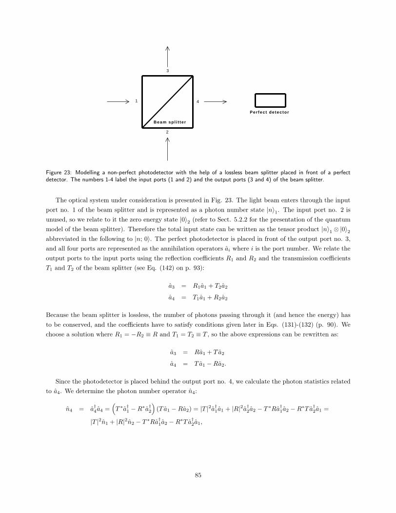
Per fect detector

Beam spl i t ter

1

2

3

4

Figure 23: Modelling a non-perfect photodetector with the help of a lossless beam splitter placed in front of a perfectdetector. The numbers 1-4 label the input ports (1 and 2) and the output ports (3 and 4) of the beam splitter.

The optical system under consideration is presented in Fig. 23. The light beam enters through the input

port no. 1 of the beam splitter and is represented as a photon number state |n〉1. The input port no. 2 is

unused, so we relate to it the zero energy state |0〉2 (refer to Sect. 5.2.2 for the presentation of the quantum

model of the beam splitter). Therefore the total input state can be written as the tensor product |n〉1 ⊗ |0〉2abbreviated in the following to |n; 0〉. The perfect photodetector is placed in front of the output port no. 3,

and all four ports are represented as the annihilation operators ai where i is the port number. We relate the

output ports to the input ports using the reflection coefficients R1 and R2 and the transmission coefficients

T1 and T2 of the beam splitter (see Eq. (142) on p. 93):

a3 = R1a1 + T2a2

a4 = T1a1 +R2a2

Because the beam splitter is lossless, the number of photons passing through it (and hence the energy) has

to be conserved, and the coefficients have to satisfy conditions given later in Eqs. (131)-(132) (p. 90). We

choose a solution where R1 = −R2 ≡ R and T1 = T2 ≡ T , so the above expressions can be rewritten as:

a3 = Ra1 + T a2

a4 = T a1 −Ra2.

Since the photodetector is placed behind the output port no. 4, we calculate the photon statistics related

to a4. We determine the photon number operator n4:

n4 = a†4a4 =(

T ∗a†1 −R∗a†2

)

(T a1 −Ra2) = |T |2a†1a1 + |R|2a†2a2 − T ∗Ra†1a2 −R∗T a†2a1 =

|T |2n1 + |R|2n2 − T ∗Ra†1a2 −R∗T a†2a1,

85

Now can find the mean number of photons emerging from the output port no. 4:

〈n4〉 = 〈n; 0| n4 |n; 0〉 = 〈n; 0|(

|T |2n1 + |R|2n2 − T ∗Ra†1a2 −R∗T a†2a1

)

|n; 0〉 = |T |2n, (121)

and the corresponding variance:

(∆n4)2

= 〈n; 0|n24|n; 0〉 − 〈n; 0|n4|n; 0〉2 = |T |4n2 + |T |2|R|2n− |T |4n2 =

|T |2|R|2n =(

1 − |T |2)

〈n4〉, (122)

where in the end we have used the fact that |R|2 + |T |2 = 1 for a lossless beam splitter, and in order to

calculate 〈n; 0|n24|n; 0〉 we have employed the commutation relation [ai, aj ] = δij . Since the detector placed

behind the output port no. 4 is assumed to be perfect, Eqs. (121)-(122) give us also the mean photocount

number and the variance of photocounts. Now, |T |2 represents the intensity transmission of the beam splitter,

so we see that high |T |2 results in low losses of the photons and vice versa. In our model |T |2 is equivalent

to the efficiency ǫ of a non-perfect detector. We observe that as |T |2 ≡ ǫ tends to 1, the measured variance

tends to zero, Eq. (122) becomes Eq. (120) and we have the sub-Poissonian photocount distribution. On

the other hand, as ǫ tends to zero and the detector becomes less and less efficient, (∆n4)2 → 〈n4〉, so the

photocount distribution degrades to the Poissonian case.

Using the same formalism it could be shown that for a coherent state input 〈n4〉 = (∆n4)2

= ǫn [104].

Thus the attenuation of the coherent light beam decreases the mean number of photocounts, but the relation

between the mean and the variance remains typical for the Poissonian distribution. This relation can be in

general quantified by introduction of the Fano factor F defined as the ratio of the variance to the mean:

F ≡ (∆n)2

〈n〉 .

We see that F = 1 for the Poissonian distribution, F < 1 for the sub-Poissonian distribution and F > 1

for the super-Poissonian distribution. Alternatively, the signal-to-noise ratio SNR might be used (Saleh and

Teich [48], Chapter 18). It is defined as:

SNR =〈n〉2

(∆n)2,

so SNR = 〈n〉 in the case of the Poissonian distribution.

We have seen how it is possible to obtain the sub-Poissonian distribution of photocounts in the corpuscular

theory. Taking into account the photon losses in the optical system, we have made a simple model where the

variance of photocounts varies smoothly between 0 and 1, something that was not possible in the semiclassical

model. Since the random selection of photons from the original stream played an important role in the above

discussion, we end it by presenting (without proof) the general formula for the final (measured) photocount

distribution P (n) given the initial distribution of emitted photons P0(r) and the total intensity transmittance

|T |2 ≡ T of the optical system (Saleh and Teich [48], Chapter 12):

P (n) =

∞∑

r=n

(

r

n

)

T r(1 − T )r−nP0(r).

86

5.1.4 Concluding remarks

In the foregoing two sections we have reviewed the theory of photocount statistics in the framework of the

semiclassical and the corpuscular model. In Chapter 4 we also examined the classical theory of optical

coherence and correlations, and in the closing paragraphs of Chapter 4.4 we presented results that follow

only from the theory of quantum correlations (i.e. when the electromagnetic field is quantized). Now we can

summarize the crucial differences between the (semi)classical and quantum models of radiation with respect

to fluctuation correlations and photocount statistics:

• Quantization of the electromagnetic field allows for weaker correlations of intensity fluctuations than are

possible within the classical model. “Weaker” must be understood in the sense of breaking inequalities

given by Eq. (104)-(105) (p. 72):

γ(2)(r, r, 0) ≥ 1

γ(2)(r, r, 0) ≥ γ(2)(r, r, ∆t 6= 0)

A situation where γ(2)(r, r, 0) < γ(2)(r, r, ∆t 6= 0) (not necessarily for all ∆t 6= 0) is commonly

interpreted as antibunching of photons.

• The semiclassical model of the photodetection process sets a lower theoretical bound for the variance,

and this bound is equal to the mean value of photocounts (Eq. (117)). The variance in the corpuscular

model, however, can be arbitrarily low (sub-Poissonian). This is due to the fact that in the corpuscular

model light may be represented in terms of the highly nonclassical photon number states, and in the

case of pure number states the variance is zero per definition (see Sect. 2.3.3). In fact, the occurence of

sub-Poissonian photocount statistics is equivalent (at least for a stationary field) to a situation where

γ(2)(r, r, 0) < 1 (Zou and Mandel, [105]).

It remains to ask whether antibunching and/or sub-Poissonian photocount statistics were observed experi-

mentally, and the answer is positive. Sub-Poissonian statistics was obtained for instance by by Short and

Mandel [106] employing resonance fluorescence of a single atom, by Teich and Saleh [107] who excited mer-

cury atoms using a regularized electron flow, and by Tapster, Rarity and Satchell [108] who used parametric

down-conversion. Antibunched light was generated (among others) by Kimble et al. [109] using resonance

fluorescence, by Kurtsiefer et al. [110] who examined single photons generated from vacancy centers in dia-

mond and by Santori et al. [111] who measured light emitted from a quantum dot. These were all instances

of nonclassical light that the (semi)classical theories could not account for38.

We immediately note, however, that the applicability of the semiclassical model is somewhat limited.

Let us focus on the photocount statistics, and let us consider a simple, but illustrative example with a

classical source. With “classical” we mean that the source is thermal (but made quasi-monochromatic using

appropriate filtering) or partially coherent (as a laser), so results of any photocount measurement performed

on emitted light should be in accordance with the semiclassical model. Let us now, however, equip the source

38Antibunching and sub-Poissonian statistics are often directly associated with each other, but in fact these two phenomenaare not equivalent [105]. In other words, γ(2)(r, r, 0) < 1 does not imply γ(2)(r, r, 0) < γ(2)(r, r, ∆t 6= 0) (for some ∆t), orvice versa.

87

with a shutter which opens and closes periodically in such a way that it remains open for time TO and then is

closed for time TC . These time durations are chosen in order to satisfy TC ≫ TO ≈ τdead where τdead is dead

time of the detector employed, and this detector may well be a single-photon counting module. If the value

of τdead is realistically chosen to lie around the order of magnitude 10−9-10−8 ns (see Ch. 6.4), the shutter

has to work very fast and the scheme may be very difficult to realize in practice, but is certainly possible in

principle.

The radiative field produced by our combination of the source and the shutter is obviously (using the

undulatory picture) a sequence of wave packets. The width of each wave packet is approximately TC and the

distance between their midpoints is TO. Such a field may be easily described classicaly. Now, when a single

wave packet reaches the detector, it will give rise to maximally one photocount (because TO ≈ τdead), and if

the radiation is intense enough, most wave packets will be registered by the detector in this way. Thus the

detector output would consist of a very regular sequence of photocounts where the variance is clearly lower

than the mean.

The paradox may be resolved easily: The semiclassical model is not able to account for such a situation,

because we have regularized the light beam and took into explicit consideration the detector dead time. It

could then be argued that in our setup we do not examine the classical light source per se, but only a radiation

field emerging from this source and prepared in a very special manner. Thus our photocount statistics would

not have any real significance.

Let us notice, however, that in the aforementioned experiments involving nonclassical light the situation

might be somewhat similar. The nonclassical light sources consist of small groups of atoms (or, preferably,

single atoms) which are resonantly and regularly excited using laser, so comparison with the shutter setup

seems appropriate. Besides, the stationarity condition – on which predictions of the different models usually

rest – is not paid explicit attention by most of the authors [106] [108] [109] [110] [111]. Teich and Saleh [107]

claim that their sub-Poisson source is stationary, but they neither elaborate on it or substantiate it. It seems

that both the stationarity condition and the detector dead time limitation should be examined with greater

care in the case of nonclassical light sources, because only if the first is fully satisfied and the latter deemed

unimportant, the semiclassical model could be unambiguously dismissed. On the other hand, one could try

to extend the semiclassical model in order to accommodate regularizing effects, and then try to apply this

modified model to nonclassical light sources. Our above example with the shutter experiment shows that

such extensions are certainly possible.

There are also other possible ways of improving the semiclassical model. One could examine the photode-

tection process itself in greater detail: seek involvement of new effects at very low intensities of impinging

light and put more emphasis on fluctuations inherent to the detector. Furthermore, the semiclassical model

is built around the very simple Eq. (112) (p. 80). Admittedly this equation can be demonstrated in a rig-

orous way, but the proof assumes that the interaction time between the electromagnetic field is much longer

than the period of the field oscillation and much shorter than the coherence time. This assumption is not

necessarily unreasonable, but nonetheless the length of the interaction time is chosen a priori. It would be

interesting to see what alternatives to Eq. (112) another choice of interaction time would yield, and whether

the semiclassical model could be modified considerably on such basis.

88

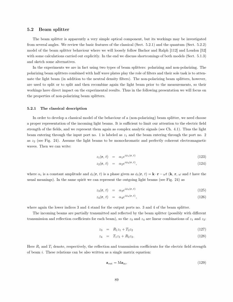
5.2 Beam splitter

The beam splitter is apparently a very simple optical component, but its workings may be investigated

from several angles. We review the basic features of the classical (Sect. 5.2.1) and the quantum (Sect. 5.2.2)

model of the beam splitter behaviour where we will loosely follow Bachor and Ralph [112] and Loudon [52]

with some calculations carried out explicitly. In the end we discuss shortcomings of both models (Sect. 5.1.3)

and sketch some alternatives.

In the experiments we are in fact using two types of beam splitters: polarizing and non-polarizing. The

polarizing beam splitters combined with half wave plates play the role of filters and their sole task is to atten-

uate the light beam (in addition to the neutral density filters). The non-polarizing beam splitters, however,

are used to split or to split and then recombine again the light beam prior to the measurements, so their

workings have direct impact on the experimental results. Thus in the following presentation we will focus on

the properties of non-polarizing beam splitters.

5.2.1 The classical description

In order to develop a classical model of the behaviour of a (non-polarizing) beam splitter, we need choose

a proper representation of the incoming light beams. It is sufficient to limit our attention to the electric field

strength of the fields, and we represent them again as complex analytic signals (see Ch. 4.1). Thus the light

beam entering through the input port no. 1 is labeled as z1 and the beam entering through the port no. 2

as z2 (see Fig. 24). Assume the light beams to be monochromatic and perfectly coherent electromagnetic

waves. Then we can write:

z1(r, t) = α1eiφ1(r, t) (123)

z2(r, t) = α2eiφ2(r, t), (124)

where αi is a constant amplitude and φi(r, t) is a phase given as φi(r, t) = k · r−ωt (k, r, ω and t have the

usual meanings). In the same spirit we can represent the outgoing light beams (see Fig. 24) as

z3(r, t) = α3eiφ3(r, t) (125)

z4(r, t) = α4eiφ4(r, t), (126)

where again the lower indices 3 and 4 stand for the output ports no. 3 and 4 of the beam splitter.

The incoming beams are partially transmitted and reflected by the beam splitter (possibly with different

transmission and reflection coefficients for each beam), so the z3 and z4 are linear combinations of z1 and z2:

z3 = R1z1 + T2z2 (127)

z4 = T1z1 +R2z2. (128)

Here Ri and Ti denote, respectively, the reflection and transmission coefficients for the electric field strength

of beam i. These relations can be also written as a single matrix equation:

zout = Mzin, (129)

89

Figure 24: A schematic illustration of a beam splitter. The input ports are represented by the left and the lower side ofthe square; the output ports by the right and the upper side. The diagonal line is an all-dielectric coating on the boundarybetween two prisms constituting the beam splitter. The coating partially reflects and partially transmits the incoming lightbeams. The light beams are represented as complex analytic signals.

with zout ≡ [z3, z4]T , zin ≡ [z1, z2]

T and M being the beam splitter matrix defined as:

M ≡[

R1 T2

T1 R2

]

.

We assume that the beam splitter is lossless, and from the energy conservation law we derive two con-

straints on the elements of M. The energy ǫi of a light beam i is proportional to the absolute square of the

related complex analytic signal zi. Thus we must have:

|z1|2 + |z2|2 = |z3|2 + |z4|2. (130)

We substitute for z3 and z4 from Eqs. (127)-(128):

|z1|2 + |z2|2 =(

|R1|2 + |T1|2)

|z1|2 +(

|T2|2 + |R2|2)

|z2|2 +

(R∗1T2 + T ∗

1R2) z∗1z2 + (T ∗

2R1 +R∗2T1) z

∗2z1.

This equation has to be valid for all z1, z2, so it yields the two constraints on the elements of the beam

splitter matrix:

|R1|2 + |T1|2 = |T2|2 + |R2|2 = 1 (131)

R1T∗2 + T1R

∗2 = 0, (132)

90

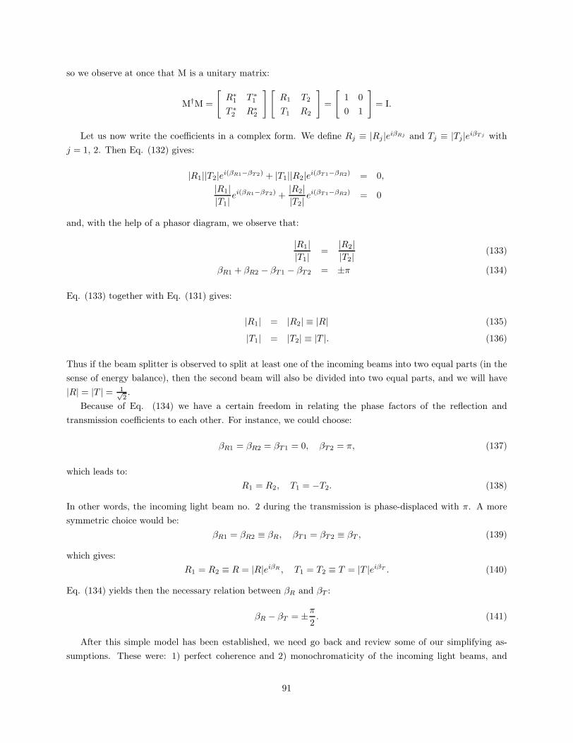
so we observe at once that M is a unitary matrix:

M†M =

[

R∗1 T ∗

1

T ∗2 R∗

2

][

R1 T2

T1 R2

]

=

[

1 0

0 1

]

= I.

Let us now write the coefficients in a complex form. We define Rj ≡ |Rj |eiβRj and Tj ≡ |Tj|eiβT j with

j = 1, 2. Then Eq. (132) gives:

|R1||T2|ei(βR1−βT2) + |T1||R2|ei(βT1−βR2) = 0,

|R1||T1|

ei(βR1−βT2) +|R2||T2|

ei(βT1−βR2) = 0

and, with the help of a phasor diagram, we observe that:

|R1||T1|

=|R2||T2|

(133)

βR1 + βR2 − βT1 − βT2 = ±π (134)

Eq. (133) together with Eq. (131) gives:

|R1| = |R2| ≡ |R| (135)

|T1| = |T2| ≡ |T |. (136)

Thus if the beam splitter is observed to split at least one of the incoming beams into two equal parts (in the

sense of energy balance), then the second beam will also be divided into two equal parts, and we will have

|R| = |T | = 1√2.

Because of Eq. (134) we have a certain freedom in relating the phase factors of the reflection and

transmission coefficients to each other. For instance, we could choose:

βR1 = βR2 = βT1 = 0, βT2 = π, (137)

which leads to:

R1 = R2, T1 = −T2. (138)

In other words, the incoming light beam no. 2 during the transmission is phase-displaced with π. A more

symmetric choice would be:

βR1 = βR2 ≡ βR, βT1 = βT2 ≡ βT , (139)

which gives:

R1 = R2 ≡ R = |R|eiβR , T1 = T2 ≡ T = |T |eiβT . (140)

Eq. (134) yields then the necessary relation between βR and βT :

βR − βT = ±π2. (141)

After this simple model has been established, we need go back and review some of our simplifying as-

sumptions. These were: 1) perfect coherence and 2) monochromaticity of the incoming light beams, and

91

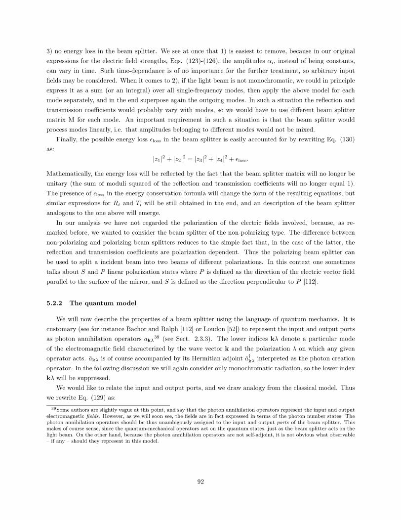
3) no energy loss in the beam splitter. We see at once that 1) is easiest to remove, because in our original

expressions for the electric field strengths, Eqs. (123)-(126), the amplitudes αi, instead of being constants,

can vary in time. Such time-dependance is of no importance for the further treatment, so arbitrary input

fields may be considered. When it comes to 2), if the light beam is not monochromatic, we could in principle

express it as a sum (or an integral) over all single-frequency modes, then apply the above model for each

mode separately, and in the end superpose again the outgoing modes. In such a situation the reflection and

transmission coefficients would probably vary with modes, so we would have to use different beam splitter

matrix M for each mode. An important requirement in such a situation is that the beam splitter would

process modes linearly, i.e. that amplitudes belonging to different modes would not be mixed.

Finally, the possible energy loss ǫloss in the beam splitter is easily accounted for by rewriting Eq. (130)

as:

|z1|2 + |z2|2 = |z3|2 + |z4|2 + ǫloss.

Mathematically, the energy loss will be reflected by the fact that the beam splitter matrix will no longer be

unitary (the sum of moduli squared of the reflection and transmission coefficients will no longer equal 1).

The presence of ǫloss in the energy conservation formula will change the form of the resulting equations, but

similar expressions for Ri and Ti will be still obtained in the end, and an description of the beam splitter

analogous to the one above will emerge.

In our analysis we have not regarded the polarization of the electric fields involved, because, as re-

marked before, we wanted to consider the beam splitter of the non-polarizing type. The difference between

non-polarizing and polarizing beam splitters reduces to the simple fact that, in the case of the latter, the

reflection and transmission coefficients are polarization dependent. Thus the polarizing beam splitter can

be used to split a incident beam into two beams of different polarizations. In this context one sometimes

talks about S and P linear polarization states where P is defined as the direction of the electric vector field

parallel to the surface of the mirror, and S is defined as the direction perpendicular to P [112].

5.2.2 The quantum model

We will now describe the properties of a beam splitter using the language of quantum mechanics. It is

customary (see for instance Bachor and Ralph [112] or Loudon [52]) to represent the input and output ports

as photon annihilation operators akλ39 (see Sect. 2.3.3). The lower indices kλ denote a particular mode

of the electromagnetic field characterized by the wave vector k and the polarization λ on which any given

operator acts. akλ is of course accompanied by its Hermitian adjoint a†kλ interpreted as the photon creation

operator. In the following discussion we will again consider only monochromatic radiation, so the lower index

kλ will be suppressed.

We would like to relate the input and output ports, and we draw analogy from the classical model. Thus

we rewrite Eq. (129) as:

39Some authors are slightly vague at this point, and say that the photon annihilation operators represent the input and outputelectromagnetic fields. However, as we will soon see, the fields are in fact expressed in terms of the photon number states. Thephoton annihilation operators should be thus unambigously assigned to the input and output ports of the beam splitter. Thismakes of course sense, since the quantum-mechanical operators act on the quantum states, just as the beam splitter acts on thelight beam. On the other hand, because the photon annihilation operators are not self-adjoint, it is not obvious what observable– if any – should they represent in this model.

92

[

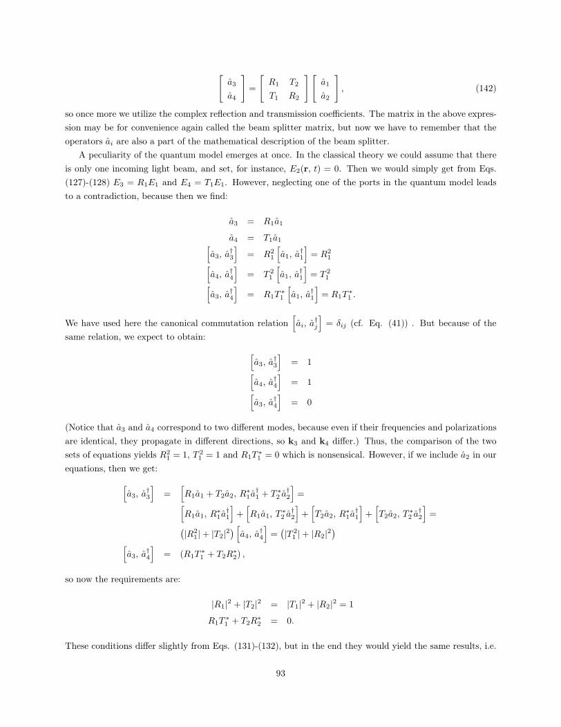
a3

a4

]

=

[

R1 T2

T1 R2

] [

a1

a2

]

, (142)

so once more we utilize the complex reflection and transmission coefficients. The matrix in the above expres-

sion may be for convenience again called the beam splitter matrix, but now we have to remember that the

operators ai are also a part of the mathematical description of the beam splitter.

A peculiarity of the quantum model emerges at once. In the classical theory we could assume that there

is only one incoming light beam, and set, for instance, E2(r, t) = 0. Then we would simply get from Eqs.

(127)-(128) E3 = R1E1 and E4 = T1E1. However, neglecting one of the ports in the quantum model leads

to a contradiction, because then we find:

a3 = R1a1

a4 = T1a1[

a3, a†3

]

= R21

[

a1, a†1

]

= R21

[

a4, a†4

]

= T 21

[

a1, a†1

]

= T 21

[

a3, a†4

]

= R1T∗1

[

a1, a†1

]

= R1T∗1 .

We have used here the canonical commutation relation[

ai, a†j

]

= δij (cf. Eq. (41)) . But because of the

same relation, we expect to obtain:

[

a3, a†3

]

= 1[

a4, a†4

]

= 1[

a3, a†4

]

= 0

(Notice that a3 and a4 correspond to two different modes, because even if their frequencies and polarizations

are identical, they propagate in different directions, so k3 and k4 differ.) Thus, the comparison of the two

sets of equations yields R21 = 1, T 2

1 = 1 and R1T∗1 = 0 which is nonsensical. However, if we include a2 in our

equations, then we get:

[

a3, a†3

]

=[

R1a1 + T2a2, R∗1a

†1 + T ∗

2 a†2

]

=[

R1a1, R∗1a

†1

]

+[

R1a1, T∗2 a

†2

]

+[

T2a2, R∗1a

†1

]

+[

T2a2, T∗2 a

†2

]

=

(

|R21| + |T2|2

)

[

a4, a†4

]

=(

|T 21 | + |R2|2

)

[

a3, a†4

]

= (R1T∗1 + T2R

∗2) ,

so now the requirements are:

|R1|2 + |T2|2 = |T1|2 + |R2|2 = 1

R1T∗1 + T2R

∗2 = 0.

These conditions differ slightly from Eqs. (131)-(132), but in the end they would yield the same results, i.e.

93

Eqs. (131)-(133). As far as the determination of the reflection and transmission coefficients is concerned,

there is a consistency between the classical and the quantum model. In the quantum model, however, the

electromagnetic fields from both input ports of the beam splitter must always be taken into consideration,

even if the light beam is being sent only through one of them. The paradox is resolved by the existence

of the omnipresent vacuum energy modes. In the absence of a “real” beam in one of the input ports (or,

equivalently, when one of the ports is closed), it is the vacuum mode that contributes to the output modes,

so we can never set a1 or a2 equal to zero.

We will now develop a simple mathematical description where one photon is being sent through the beam

splitter. The evolution through the beam splitter is represented by a unitary operator U . Let us denote by

|n〉i=1, 2 the photon number state of the light beam with n photons entering the input port no. i = 1, 2, and

by |n〉j=3, 4 the state with n photons leaving through the output port no. j = 3, 4. Thus |1〉1 |0〉2 represents

a state with one photon entering through the input port no. 1 and none entering through the input port no.

2. We examine how the beam splitter acts on |1〉1 |0〉2:

U |1〉1 |0〉2 = U a†1 |0〉1 |0〉2 = U a†1

(

U †U)

|0〉1 |0〉2 = U a†1U† |0〉3 |0〉4 ,

where the last equality is a logical consequence of the fact that if no photons are sent into the beam splitter,

then surely none will emerge from it (the number of photons is preserved). U a†1U† represents the time-

reversed evolution through the beam splitter, so with the help of Eq. (142) we represent a†1 in terms of a†3and a†4, and obtain:

U a†1U† |0〉3 |0〉4 =

(

R∗1a

†3 + T ∗

1 a†4

)

|0〉3 |0〉4 = R∗1 |1〉3 |0〉4 + T ∗

1 |0〉3 |1〉4 .

The result is a superposition of two photon number states: In the first one the input photon leaves through

the output port no. 3, and in the second one the input photon leaves through the output port no. 4. The

probability amplitudes of the superposition are the complex conjugates of the appropriate reflection and

transmission coefficients. Given the postulated indivisibility of the photons, such a result could be intuitively

expected.

Let us now consider a situation where two photons are sent into the beam splitter, one through each input

port40, so the input photon number state is |1〉1 |1〉2. We have:

U |1〉1 |1〉2 = U a†1a†2 |0〉1 |0〉2 = U a†1U

†U a†2U†U |0〉1 |0〉2 =

(

U a†1U†)(

U a†2U†)

|0〉3 |0〉4 =(

R∗1a

†3 + T ∗

1 a†4

)(

T ∗2 a

†3 +R∗

2a†4

)

|0〉3 |0〉4 =√

2R∗1T

∗2 |2〉3 |0〉4 +

√2T ∗

1R∗2 |0〉3 |2〉4 + (R∗

1R∗2 + T ∗

1 T∗2 ) |1〉3 |1〉4

We remember that the coefficients must satisfy some specific conditions. Using, for instance, Eq. (137)-(138),

40It seems natural to require that the photons are present at both inputs at the same time. Notice, however, that the timeaspect is altogether absent in this rather crude model. When we work with the photon number states, we have to consider theoptical field in its totality, and we are unable to track the propagation of single photons through space (see the remarks in Sect.2.3.4). We will come back to this issue in the next section.

94

and assuming that we are using a 50:50 beam splitter (where |Ri| = |Ti| = 1√2), we obtain:

U |1〉1 |1〉2 =1√2|2〉3 |0〉4 +

1√2|0〉3 |2〉4 . (143)

Thus, with right conditions, there will occur a situation where we send one photon through each of the input

ports, and the resulting state will be a superposition of |2〉3 |0〉4 and |0〉3 |2〉4. The subsequent measurement

of the output arms will either show that both photons have left the beam splitter through the output port no.

3, or that the photons have left through the port no. 4. We will not, however, observe the case where there

are single photons in each output, because the term |1〉3 |1〉4 has cancelled. This is an example of quantum

interference effect. We notice that this quantum interference could be discussed in the context of quantum

entanglement of which the RHS of Eq. (143) is an instance. As remarked in the Introduction, the complex

subject of the quantum entanglement lies outside the scope of the thesis, so we will not follow this line of

reasoning further.

We examine also the case of the beam splitter acting on an coherent state |z〉 in one of the input ports.

We will make use of the shift operator D(z) defined in Appendix B.3 (Eq. (197)):

U |z〉1 |0〉2 = UD1(z) |0〉1 |0〉2 = UD1(z)U†U |0〉1 |0〉2 = UD1(z)U

† |0〉3 |0〉4 = U(

eza†1−z∗a1

)

U † |0〉3 |0〉4 =(

ezR∗1 a†

3+zT∗1 a†

4−z∗R1a3−z∗T1a4

)

|0〉3 |0〉4 = (ezR∗1 a†

3−z∗R1a3)(

ezT∗1 a†

4−z∗T1a4

)

|0〉3 |0〉4 =

D (zR∗1) D (zT ∗

1 ) |0〉3 |0〉4 = |zR∗1〉3 |zT ∗

1 〉4

The factorization of exponentials was possible because[

a3, a†4

]

= [a3, a4] = 0. We see that output state is a

product of coherent states. In a similar way we can calculate the output state when there are two different

coherent states entering the input ports of the beam splitter, |zA〉 and |zB〉. The final result is:

U |zA〉1 |zB〉2 = e(z∗AzBR1T∗

2 −zAz∗BR∗

1T2)/2 |zAR∗1 + zBT

∗2 〉3 |zAT

∗1 + zBR

∗2〉4 .

The output state is again a product of coherent states, but this time the input coherent states are mixed in

the output, and there is an additional phase factor.

5.2.3 Shortcomings of the beam splitter model

After having presented the basic features of the classical and the quantum beam splitter, we would like

now to point out and discuss shortcomings of both models. We are not claiming that they are erroneous in

any direct way. The models have been succesfully applied in the descriptions of many different experiments,

and they are also essential elements of the frameworks of larger optical and quantum-optical theories. We

will rather try to make a case that there are certain subtle, unclear aspects of the models that may bear

relevance when one examines the nature of light by experimental means.

To begin with we notice that the beam splitter is treated as a black box. It is described in terms of

its transfer characteristics which, given an input state, produce an output state. The models say almost

nothing about the internal workings of the beam splitter. One could of course argue that a beam splitter is

essentially a half-silvered mirror, so no detailed description of such simple a device should be ever needed.

95

However, exactly the same line of reasoning shows that the workings of the beam splitter is intimately

connected with the principles governing the interaction between light and matter. After all, the half-silvered

mirror is supposed to absorb the radiation incoming from two directions and then re-emit it again in two other

directions. Since the issue of the light-matter interactions is given a lot of detailed thought in other situations

(like the photoelectric effect, see Ch. 3.3; not to mention the whole theory of quantum electrodynamics),

there is no reason for not raising it in the case of the beam splitter.

This lack of interest in the inner workings of the device is made apparent by the constancy of the reflection

and transmission coefficients, Ri=1, 2 and Ti=1, 2. These coefficients are completely indepedent of the incoming

radiation fields, and they neither possess any explicit time-dependence. This may seem unjustified when we

recall that the electrons consistuting the mirror of the beam splitter absorb and re-emit the radiation involved,

so the dynamical properties of the electrons surely need to influence the whole process of beam splitting. On

the other hand, these very properties are influenced by the radiation, so it is reasonable to believe that the

characteristics of the radiation fields affect the way the fields themselves are divided inside the beam splitter.

In other words, the description in terms of constant coefficients could be well appropriate in the equilibrium,

but as soon as the first “segment” (however we define it) of the electromagnetic field irradiates the beam

splitter, its behaviour changes and the next “segments” are processed differently. The aforementioned explicit

time-dependence would be caused by the fact that even in the absence of any radiation the beam splitter

system is not in a perfect equilibrium, but, for instance, oscillates around it in the phase space due to thermal

influences.

In order to illustrate this problem, let us take a look at the classical model, and imagine that an electro-

magnetic field enters the beam splitter through the input port no. 1. We represent again the electromagnetic

field with the help of the complex analytic signal z1(r, t) where z1(r, t) may be a general function of position

and time. As noticed before, the field is split into z3 = R1z1 leaving through the port no. 3 and z4 = T1z1

leaving through the port no. 4. Thus the splitting of the original field is ideal, because the form of z1 is not

changed at all ; and besides no fluctuations are introduced due to the interaction with the beam splitter41.

From the strictly practical point of view, such ideal splitting is impossible. One could argue that any addi-

tional effects caused by the beam splitter, even if present, are minute, so there is no need for taking them

into account. This is certainly true in experiments where the process of beam splitting is only a minor part

of the general setup, and where during any single measurement of the spli beam we integrate over relatively

long time scales. However, in the experiments examining the wave-particle duality, the beam splitter is often

the central element of the setup (as in coincidence measurements, or in a Mach-Zender interferometer), and

the time scales corresponding to the passage of a “single photon” or a “single wave packet” may be very short.

This leads us to the question whether a more elaborate model of the beam splitter would allow us to interpret

the results of these experiments differently.

We will now consider one simple way the existing classical beam splitter model could be improved. It

is not our goal to develop here a complete description, but only to show how the mathematics might be

modified. We introduce the dependence on the electromagnetic field explicitly into the coefficients. For

instance, the reflection coefficient R1 could be written:

R1 = const. → R1(t) = R1,0 + fR1 [z1(t− τ), z2(t− τ)]

41Of course the original fluctuations will be transmitted through the beam splitter (and if there were two input fields, theirfluctuations will be also mixed in the output). However, no new fluctuations will be produced.

96

where R1,0 is the original constant value and fR1 represents the change due to the influence of the input fields

z1 and z2 at time t − τ where t is the time the value of R1 is calculated for. More realistically, fR1 should

not depend on any single past values of z1 and z2, because the influence is continuous. Thus we would write:

R1(t) = R1,0 + fR1 (S)

where S is the integral:

S =

∫ t

t−τ

g(t′

)h[

z1(t′

), z2(t′

)]

dt′

.

Here g(t′

) is an appropriate weighting function, and h[

z1(t′

), z2(t′

)]

decides how the past values of electric

field strenghts contribute to the present behaviour of the beam splitter. fR1 would be then used in order

to calculate the contribution of the integral to R1. Notice that τ would correspond to the relaxation time,

and that the maximal value of fR1 (S1, S2) should be much smaller than R1,0 – because, as remarked before,

such additional beam splitter effects must be minute. Similar relations to that for R1(t) could be derived

for R2(t), T1(t) and T2(t). In the case of the lossless beam splitter the constraints given by Eqs. (131)-(132)

are assumed to be still valid, so these could be used in order to examine the relations between R1,0, R2,0,

fR1 , fR2 and so on. Deducing the actual form of all these new function would not be an easy task. Apart

from “intelligent guessing”, one could try to apply principles of quantum electrodynamics describing the light-

matter interactions. Then we would have to look for any new predictions regarding the behaviour of the

beam splitter and try to confirm them (or refute) empirically42.

In the case of the quantum model, the same remarks still apply, because the reflection and transmission

coefficients are used here as well (as a matter of fact they are taken directly from the classical model). In

addition, however, there is the problem of the Fock states being unable to say anything about how positions

of single photons change with time. As noted in Section 2.3.4, the photon number states formalism treats the

electromagnetic field holistically. Consider, for instance, the situation described by Eq. (143). The model

tells us that if one photon enters the beam splitter through the input port no. 1, and another one through

the input port no. 2, and if we place two perfect detectors in front of the output ports, then we will either

register two photons leaving the beam splitter through the output port no. 3, or two photons leaving through

the output port no. 4. It is striking that the model do not make any claims on the original photons entering

the beam splitter simultaneously43. Thus we do not know what is the maximal time interval allowed between

these two events, and how the time difference involved would affect the output state (if at all). We do not

know neither how the photons in the output state will be distributed in time.

In many experimental situations these kinds of information may be unnecessary for the correct prediction

of the results. However, the same cannot be said about the experiments regarding the wave-particle duality.

There are three reasons for this state of affairs. First and foremost, in order to resolve (or at least understand

better) the duality problem, we crave to gain an intimate knowledge about what happens with a segment of

42Another possibility worth considering would be to model the beam splitter in terms of driven harmonic oscillations: z3 +bz3 +kz3 = f(z1, z2), where z3 is an output field, b and k are constants, and the function f(z1, z2) describes the influence of theinput fields. The emergence of resonance for some specific z1 and z2 would reflect the fact that the reflection and transmissioncoefficients vary with modes, particularly with the wavelength, as seen in Fig. 33 on p. 112. Furthermore, some choices of thefunction f would naturally lead to interesting additional effects, also at low intensities of the incoming fields.

43Unless this simultaneity requirement is implicitly present in a definition of a state like |1〉1 |1〉2, i.e. unless we read |1〉1 |1〉2as “a situation where a photon number state |1〉 enters the input port no. 1 and at the same time another photon number state|1〉 enters the input port no. 2”. However, this solution cannot be applied to cases with photon number states |n > 1〉, becausewe cannot require that all n photons from a photon number state |n > 1〉 are present at the same point in spacetime.

97

a light beam44 between its emission from the source and its detection at the source. Any shortcomings of

the quantum model as problematic as the ones mentioned in the previous paragraph could hardly help us in

achieving such knowledge. Secondly, the experiments involving the wave-particle duality rely heavily on coin-

cidence and interferometry measurements where the time aspect plays a prominent role. Any improvements

on the model which would stop treating “photons” holistically could thus help us in predicting, describing

and quantifying possible new effects. And, finally, such holistic approach to the electromagnetic field is of no

help when we try to understand better the nature of a “photon”, because it does not allow us to speculate

about what “photon” is.

We note that the critical remarks from the last two paragraphs do not apply only to the quantum model

of the beam splitter, but to the photon number states formalism on which this model is based. This is an

important point, because the successes the corpuscular theory of light have achieved on the quantitative

field make us easily forget that the same theory has serious problems when it comes to answering qualitative

questions about the physical reality of different phenomena. It is curious that the situation of the classical

model of light may be seen as the reverse of the situation of the quantum model – the (semi)classical model

is (so far) not able to properly predict all experimental results (see Sect. 5.1.4), but it presents us with a

much clearer physical picture of the beam splitting process. If we refer to the three items from the previous

paragraph, we see that 1) the classical model assumes that the light beam propagates from the source to the

detector as an electromagnetic wave, or, more precisely, as a wavelike variation of the electromagnetic field;

2) the propagation of this electromagnetic wave can be easily analyzed as a function of time; and 3) the light

may be depicted as an electromagnetic wave with varying degree of coherence (see Chapter 4).

We conclude the above section by saying that there is room for improvement in both the classical and

the quantum model of the beam splitter. However, while an improvement of the classical model could be

achieved by introducting new factors to the model without revising the underlying theory of light, an im-

provement of the quantum model will likely require us to modify some elements of its theoretical foundations.

5.3 The shape of the laser beam

The aim of the following section is to give a quantitative description of the laser beam shape. First we

show how one can spatially confine an ordinary plane wave using an appropriate envelope. We derive the

paraxial Helmholtz equation that the envelope has to satisfy (Sect. 5.3.1). Then we present a simple solution

of the equation which embodies the complex envelope of the Gaussian beam; the subsequent analysis of the

expression for the complex amplitude allows us to recognize several quantities of physical significance (Sect.

5.3.2). Also, we quickly review the ABCD law which is an important tool in examining how different optical

elements influence the Gaussian beam (Sect. 5.3.3).

In our presentation we follow mainly Saleh and Teich [48] and Milonni and Eberly [100], but the formula

for the complex amplitude of the Gaussian beam, Eq. (157), will be derived more explicitly than it is usually

done.

Note that this chapter is rather technical and we aim at establishing the mathematical theory that will

be used in Chapter 5.3.3. Specifically, the shape of the laser beam will not be discussed in the context of the

wave-particle duality as different models of photodetection (Section 5.1.4) and beam splitters (Sect. 5.2.3)

were.44The phrase “segment of a light beam” may sound artificial in this context, but we want to avoid the terms “wave packet” or

“photon” which suggest undulatory or corpuscular view of light, respectively.

98

5.3.1 The paraxial Helmholtz equation

In terms of the classical theory the laser beam consists of an electromagnetic field propagating undulatorily

through space, the laser being its source. The electromagnetic field has to satisfy the Maxwell equations, Eq.

(2.1)-(2.4), and thus the wave equation, Eq. (2.10), or, alternatively, Eq. (2.11). In the following we will use

the latter form:

∇2u− 1

v2

∂2u

∂t2= 0. (144)

We recall that u denotes any component of the electric or magnetic field constituting the beam, and v is the

phase velocity of the component. This velocity is generally given as v = cn , where c is the speed of light in

vacuum and n is the refractive index of the medium. Eq. (144) has to be satisfied for all six components

(three electric and three magnetic), but we will focus on only one of them, the treatment of the other five

being completely similar. Thus the scalar function of position r and time t, u(r, t), can for instance represent

a single component of the electric field. u(r, t) is sometimes called the wavefunction (not to be confused with

the wave function of quantum mechanics). It could be represented with the help of the complex analytic

signal (see Ch. 4.1), but it is unnecessary to apply the formalism of the complex analytic signal in the

discussion of the laser beam shape.

We saw in Chapter 2.1 that the simplest solution of the wave equation is a plane wave described by a

vector parameter k (the wave vector) related to the spatial argument, and a scalar parameter ω (the angular

frequency) related to the temporal argument. But obviously these solutions, given by Eqs. (2.13)-(2.14),

cannot be applied in the case of the laser beam, because the laser beam is strongly limited in space, i.e. the

wavefunction has to tend rapidly to zero outside some relatively narrow region (see the remark in Ch. 3.2).

Specifically, we need a solution that gives us a paraxial wave characterized by a wavefront normal which

makes a small angle with the optical axis of the system (the propagation axis). Also, the paraxial wave needs

lie close to the axis. Such a solution can be obtained by modulating a plane wave solution with a proper

position-dependent envelope A(r). If we choose the z-axis of the coordinate system to be the optical axis of

our model, we get:

u(r, t) = A(r)e−j(kz−ωt) . (145)

It remains to see what conditions constrain A(r) so Eq. (144) is satisfied. First and foremost, the envelope

has to vary slowly in the z-direction within a distance that is small relatively to the wavelength λ = 2πk ,

because we want the wavefunction to resemble a plane wave (propagating in the z-direction) at small spatial

scale. The partial derivatives ∂A∂z must change slowly for the same reason. If ∆A denotes the change of A

within a small (i.e. equal to the wavelength) distance ∆z in the positive z-direction, we have:

|∆A| =

∣

∣

∣

∣

∂A

∂z

∣

∣

∣

∣

∆z =

∣

∣

∣

∣

∂A

∂z

∣

∣

∣

∣

λ≪ |A| ⇒∣

∣

∣

∣

∂A

∂z

∣

∣

∣

∣

≪ |A|λ

∼ k|A|. (146)

Similarly, if ∆∂A∂z denotes the change of the partial derivative of A, we obtain:

∣

∣

∣

∣

∆∂A

∂z

∣

∣

∣

∣

=

∣

∣

∣

∣

∂2A

∂z2

∣

∣

∣

∣

∆z =

∣

∣

∣

∣

∂2A

∂z2

∣

∣

∣

∣

λ≪∣

∣

∣

∣

∂A

∂z

∣

∣

∣

∣

≪ k|A| ⇒∣

∣

∣

∣

∂2A

∂z2

∣

∣

∣

∣

≪ k|A|λ

∼ k2|A|, (147)

(If A(r, t) is a complex function, as is usually the case, the inequalities have to apply separately to the

99

absolute values of real and imaginary parts.) We substitute now from Eq. (145) in Eq. (144):

∇2[

A(r)e−j(kz−ωt)]

− 1

v2

∂2

∂t2

[

A(r)e−j(kz−ωt)]

=

(∇2TA)e−j(kz−ωt) +

∂

∂z

[

∂A

∂ze−j(kz−ωt) − jkAe−j(kz−ωt)

]

+Aω2

v2e−j(kz−ωt) =

[

∇2TA+

∂2A

∂z2− 2jk

∂A

∂z− k2A+A

ω2

v2

]

e−j(kz−ωt) = ∇2TA− 2jk

∂A

∂z= 0

∇2T is the transverse Laplacian, ∇2

T ≡ ∂2

∂x2 + ∂2

∂y2 , and in the second to last transition we have set ωv = k and

we have neglected ∂2A∂z in accordance with Eq. (147). Thus we have obtained a differential equation that the

envelope A(r) needs to satisfy:

∇2TA(r) − 2jk

∂A(r)

∂z= 0. (148)

The equation is called the slowly varying envelope approximation of the Helmholtz equation or the paraxial

Helmholtz equation.

5.3.2 The Gaussian beam

A possible solution of Eq. (148) is the paraboloidal wave:

A(r) =A1

ze−jk x2+y2

2z , (149)

with A1 being a constant. The validity of the paraboloidal solution as a possible envelope can be checked by

direct substitution from Eq. (149) into (148). By defining ρ2 ≡ x2 + y2 it is possible to derive an auxillary

expression:

∇2T f(ρ2) = 4[ρ2f

′′

(ρ) + f′

(ρ)]

where prime denotes differentiation with respect to ρ2. Then we obtain:

∇2TA(r) = 4

[

−ρ2 k2

4z2A(r) − jk

2zA(r)

]

=

[

−ρ2k2

z2− 2jk

z

]

A(r)

2jk∂A(r)

∂z= 2jk

[

−1

zA(r) + jk

ρ2

2z2A(r)

]

=

[

−2jk

z− ρ2k2

z2

]

A(r)

and the paraxial Helmholtz equation is obviously satisfied, the difference of both terms being identically zero.

It is, however, not the paraboloidal envelope that is most often used to model the laser beam, but the

Gaussian envelope. The Gaussian solution can be simply obtained from the paraboidal one by substituting

z with q(z) ≡ z − ξ. If ξ is real, this corresponds to a trivial shift of the point z on the z-axis about which

the paraboloidal wave is centered in the xy- or the xz-plane (from z = 0 to z = ξ). However, ξ can be also

taken to be complex, and then the new solution acquires altogether new properties. Choosing ξ to be purely

imaginery, say ξ = −jz0, results in the complex envelope of the Gaussian beam:

A(r) =A1

q(z)e−jk ρ2

2q(z) , q(z) = z + jz0 (150)

100

q(z) is known as the q-parameter of the Gaussian beam, and z0 as the Rayleigh range.

The exponent in Eq. (150) is now not purely imaginery, but complex. Let us separate explicitly the real

and the imaginary part of q−1(z):

1

q(z)=

1

z + jz0=

z

z2 + z20

− jz0

z2 + z20

≡ α− jβ (151)

We insert the expression for q−1(z), Eq. (151), into Eq. (150):

A(r) = A1(α − jβ) exp

[

−jk ρ2

2α

]

exp

[

−kρ2

2β

]

. (152)

The complex number in the prefactor can be written in exponential form: α − jβ = Wejζ where both W

and ζ are functions of the position z:

W (z) ≡√

α2 + β2 =1

√

z2 + z20

=1

z0√

1 + z2

z20

ζ(z) ≡ arctan

(

−βα

)

= arctan(

−z0z

)

= arctan

(

z

z0

)

− π

2

We may now write α and β as:

α =z

z2 + z20

= zW 2(z) ≡ 1

R(z)(153)

β =z0

z2 + z20

= z0W2(z) ≡ λ

πW 2(z)(154)

These curious definitions will be justified shortly, as we will see that the quantities R(z) and W (z) are of

physical significance. Eq. (152) can be now expressed as:

A(r) = A1Wejζ exp

[

−jk ρ2

2R(z)

]

exp

[

− ρ2

W 2(z)

]

(155)

From Eq. (154) we extract the relationship between W (z) and W (z):

W (z) =

√

λ

πz0

1

W (z)=

√

λz0π

√

1 +z2

z20

≡W0

√

1 +z2

z20

where W0 ≡√

λz0

π . Eq. (155) becomes:

A(r) =A1

z0

W0

W (z)exp

[

− ρ2

W 2(z)

]

exp

[

−jk ρ2

2R(z)+ jζ(z)

]

=

A1

jz0

W0

W (z)exp

[

− ρ2

W 2(z)

]

exp

[

−jk ρ2

2R(z)+ jζ(z)

]

≡

A0W0

W (z)exp

[

− ρ2

W 2(z)

]

exp

[

−jk ρ2

2R(z)+ jζ(z)

]

(156)

101

where we have defined

A0 ≡ A1

jz0, ζ(z) ≡ arctan

(

z

z0

)

Substituting for the envelope from Eq. (156) in the wavefunction, Eq. (145), yields our final result:

u(r, t) = A0W0

W (z)exp

[

− ρ2

W 2(z)

]

exp

[

−jkz − jkρ2

2R(z)+ jζ(z)

]

exp(jωt), (157)

which is the complex amplitude of the Gaussian beam. Eq. (157) must be considered together with the

formulas for beam parameters W (z), W0, R(z) and ζ(z):

W (z) = W0

√

1 +z2

z20

(158)

W0 =

√

λz0π

(159)

R(z) = z

(

1 +z20

z2

)

(160)

ζ(z) = arctan

(

z

z0

)

(161)

The physical meaning of these parameters can be inferred from Eq. (157). W (z) is a radial measure of

the beam width, because we see that the term e−ρ2/W 2(z) will attenuate the amplitude when we move away

from the optical z-axis (i.e. when ρ2 = x2 + y2 grows). The beam width, however, depends on the position

along the z-axis, and since it increases with increasing |z|, the beam will diverge as we move away from the

plane z = 0. At that plane the beam width is yielded by W0. z = 0 is the so-called beam waist, and W0 is

called the waist radius.

At z = z0 the beam width W (z) assumes the value√

2W0. Thus we see that the Rayleigh range z0is the scaling factor for the divergent behaviour of the beam. The depth of focus (also known as confocal

parameter) is defined as twice the Rayleigh range:

rd.o.f. ≡ 2z0 =2πW 2

0

λ. (162)

R(z) represents the wavefront radius of curvature. This is not seen directly from Eq. (157), and a more

careful analysis is needed [100]. We notice that R(z) is infinite at the beam waist, so the wavefronts are

planar there. R(z) obtains a minimum, 2z0, at z = ±z0, and when z ≫ z0 the radius of curvature increases

linearly with z.

Finally, ζ(z) is the phase retardation brought in by the envelope, known as the Gouy phase [101]. It

ranges from −π2 at z → −∞ to π

2 at z → ∞.

Two other important quantities can be determined with the help of Eqs. (157)-(161). The first of these

is the optical intensity I of the beam:

I(ρ, z) = |u(r, t)|2 =I0W

20

W 2(z)exp

[

− 2ρ2

W 2(z)

]

, I0 ≡ |A0|2. (163)

We see now clearly that the intensity decrease is caused at all z by a Gaussian function, with the radial

distance ρ as the argument. Hence the name of the beam. We can easily calculate the total optical power

102

carried by the beam at any transverse plane:

P (z) =

∫ ∞

0

∫ 2π

0

I(ρ, z) ρ dφ dρ = 2π

∫ ∞

0

I(ρ, z) ρ dρ =2πI0W

20

W 2(z)

∫ ∞

0

ρ exp

[

− 2ρ2

W 2(z)

]

dρ =

=πI0W

20

W 2(z)

∫ ∞

0

exp

[

− 2u

W 2(z)

]

du =1

2πI0W

20 =

1

2I0(πW

20 ),

so the total optical power is half the maximal intensity multiplied by the beam waist area (defined as the

circle with radius equal to the waist radius W0).

Let us also find the divergence angle of the Gaussian beam. From Eq. (158) we see that when z ≫ z0,

the beam diverges linearly as:

W (z) ≈W0z

z0≡ z sin θ,

with the definition sin θ ≡ W0

z0for the divergence angle θ. However, usually we have W0 ≪ z0 (the waist

radius is much smaller than the Rayleigh range), so we obtain:

θ =W0

z0=

1

z0

√

λz0π

=λ

πW0. (164)

Thus a highly directional laser beam can be obtained by using a short wavelength and a large waist radius.

5.3.3 The ABCD law

The shape of the Gaussian beam is completely described by the beam width W (z) and by the wavefront

curvature radius R(z). These quantities, given that the wavelength λ is known, can be determined from the

q-parameter, Eq. (151). Using it together with Eqs. (153)-(154) we get:

1

q(z)=

1

R(z)− j

λ

πW 2(z).

The shape of the beam changes both during propagation in a homogenous medium (as seen from Eqs.

(158) and (160)) and due to a transfer through some optical component, a thin lens and a curved interface

being probably the most important examples. In the latter case it can be demonstrated (cf. Milonni and

Eberly [100] or Gerrard and Burch [113]) that the beam remains Gaussian, but its q-parameter is transformed,

q → q′

, in accordance with the ABCD law:

q′

=Aq +B

Cq +D, (165)

where A, B, C and D are parameters describing the given optical component. These parameters can be

collected in a matrix M :

M =

[

A B

C D

]

.

For a thin lens of focal length f the matrix is:

MTL =

[

1 0

− 1f 1

]

,

103

and for a refraction at curved interface:

MCI =

[

1 0n1−n2

Sn2

n1

n2

]

,

where S is the curvature radius (with centre of curvature after the interface), n1 is the initial index of

refraction and n2 is the final index of refraction. If the interface is flat, S → ∞ and MCI becomes diagonal.

Eq. (165) applies also when the beam propagates in a homogenous medium. Then the appropriate matrix

is:

MP =

[

1 d

0 1

]

with d being the optical length, i.e. the physical length multiplicated with the refractive index of the medium.

In the case of propagation in free space the application of Eq. (165) is obviously equivalent with the straight-

forward formulas given by Eq. (158) and Eq. (160).

The relevance of the matrix representation of the optical elements is contained in the mathematical fact

that this representation is invariant to cascading of the elements. If we have a system consisting of many

optical elements labeled by numbers 1, 2, 3, . . . , n, where the labeling reflects the succession of the elements,

the influence of the whole system on the Gaussian beam can be described simply by a matrix MTOT being

the product of the matrices representing the elements separately:

MTOT = Mn . . .M3M2M1.

The free space between elements have to be included as optical elements on their own, making use of MP

above.

The method described above, i.e. the ABCD law combined with the matrix representation of the optical

elements, is a popular technique used for designing and analyzing optical systems. The calculations involved,

however, are tedious from the algebraic point of view, so usually they are carried out numerically with the

help of an appropriate computer program.

For the sake of completeness we notice that the method is closely related to another important technique

in ray optics where one wants to trace a paraxial ray using two variables, r and φ. r is the transverse offset of

the ray and φ the offset angle (both measured relatively to the optical axis). These variables are collected as

a vector [r φ]T which the optical elements transform through an ordinary matrix multiplication. The matrix

representation of these elements are the same as for the Gaussian beam, and the cascading invariance still

applies.

104

6 The main elements of the experimental setup: specifications and

preliminary measurements

After the purely theoretical treatment of the previous chapter, we will here give specifications of the laser

(Tab. 1 on p. 106), the non-polarizing beam splitters (Tab. 2 on p. 111) and the detectors (Tab. 3 on p.

114) used in our experimental setup. Furthermore we will present results of some preliminary measurements

regarding the laser and the detectors. First we measure and model the laser beam; we demonstrate that

it is indeed approximately Gaussian, we describe it graphically and we determine its parameters (Ch. 6.1).

Then we will measure the coherence length of the beam (Ch. 6.2) using the principle presented in Ch. 4.4.

Afterwards we give specifications of our non-polarizing beam splitter (Ch. 6.3) and experimentally verify that

for our photodetectors the response to the impinging radiation is linear (in the low photocount rate regime)

(Ch. 6.4). Finally we measure the photocount statistics, demonstrate that it is Poissonian and determine

the afterpulse probability of the detector (Ch. 6.5).

6.1 Modelling the laser beam shape

We are using a helium-neon laser produced by Thorlabs. The specifications are given in Tab. 1. The

output power was measured to be ca. 12.1 mW approximately 10 cm from the output coupler. We were

using pyrroelectric energy sensor ES120 [121] connected to digital power metre console PM100 [122] (both

manufactured by Thorlabs).

We proceed to measure the transverse profile of the laser beam. Here, we use a CCD device, and the

beam has to be attenuated with neutral density filters (NDF) in order to avoid saturation of the CCD.

NDF’s, as any other optical element, will distort the beam profile. In the case of NDF’s this is due to several

factors. The filters used in the experiment do not have anti-reflective coatings, so stray light has not been

reduced. Besides, we assemble and align the optical components manually, and it is impossible to achieve an

alignment that is completely perpendicular to the optical axis. The third reason is that the filter surfaces are

not perfectly homogenous, since the absorbing substance that covers the glass is granular at the microscopic

scale.

We check qualitatively how large the distortion actually is already at this introductory stage, since during

the experiment it will be crucial to obtain an even stronger attenuation with several NDF’s, Therefore the

CCD is used to measure45 the profile of the beam attenuated with one and with four NDF’s, the total45Notice, however, that we have assumed a linear response of the CCD to the incoming light intensity, at least in the intensity

105

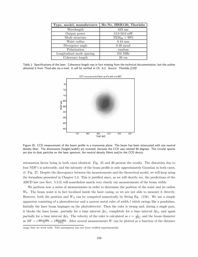
Type, model, manufacturer He-Ne, HRR120, Thorlabs

Wavelength 633 nmOutput power 12.0-50.0 mWMode structure TEM00 > 99%Waist radius 0.44 mm

Divergence angle 0.46 mradPolarization random

Longitudinal mode spacing 316 MHzCoherence length 20 cm

Table 1: Specifications of the laser. Coherence length was in fact missing from the technical documentation, but the authorobtained it from ThorLabs via e-mail. It will be verified in Ch. 6.2. Source: Thorlabs [120]

Figure 25: CCD measurement of the beam profile in a transverse plane. The beam has been attenuated with one neutraldensity filter. The dimensions (height/width) are reversed, because the CCD was rotated 90 degrees. The circular specksare due to dust particles on the laser aperture, the neutral density filters and/or the CCD device.

attenuation factor being in both cases identical. Fig. 25 and 26 present the results. The distortion due to

four NDF’s is noticeable, and the intensity of the beam profile is only approximately Gaussian in both cases,

cf. Fig. 27. Despite the discrepancy between the measurements and the theoretical model, we will keep using

the formalism presented in Chapter 5.3. This is justified since, as we will shortly see, the predictions of the

ABCD law (see Sect. 5.3.3) will nonetheless match very closely our measurements of the beam width.

We perform now a series of measurements in order to determine the position of the waist and its radius

W0. The beam waist is in fact localized inside the laser casing, so we are not able to measure it directly.

However, both the position and W 0 can be computed numerically by fitting Eq. (158). We use a simple

apparatus consisting of a photodetector and a narrow metal ruler of width l which swings like a pendulum.

Initially the laser beam impinges on the photodetector. Then the ruler is swung and, during a single pass,

it blocks the laser beam: partially for a time interval ∆t1, completely for a time interval ∆t2, and again

partially for a time interval ∆t3. The velocity of the ruler is calculated as v = l∆t2

, and the beam diameter

as 2W = v∆t1+∆t32 = l∆t1+∆t3

2∆t2. After several measurements W can be plotted as a function of the distance

range that we work with. This assumption has not been verified experimentally.

106

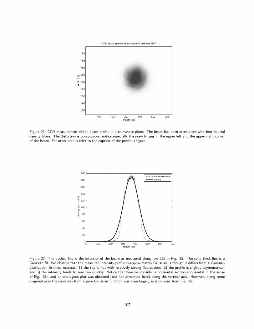
Figure 26: CCD measurement of the beam profile in a transverse plane. The beam has been attenuated with four neutraldensity filters. The distortion is conspicuous; notice especially the skew fringes in the upper left and the upper right cornerof the beam. For other details refer to the caption of the previous figure.

0 100 200 300 400 500 600 7000

20

40

60

80

100

120

140

160

180

200

Height [px]

Inte

nsity

[arb

. uni

ts]

measurementstheory

Figure 27: The dashed line is the intensity of the beam as measured along row 225 in Fig. 25. The solid thick line is aGaussian fit. We observe that the measured intensity profile is approximately Gaussian, although it differs from a Gaussiandistribution in three respects: 1) the top is flat with relatively strong fluctuations, 2) the profile is slightly asymmetrical,and 3) the intensity tends to zero too quickly. Notice that here we consider a horisontal section (horisontal in the senseof Fig. 25), and an analogous plot was obtained (but not presented here) along the vertical axis. However, along somediagonal axes the deviation from a pure Gaussian function was even larger, as is obvious from Fig. 25.

107

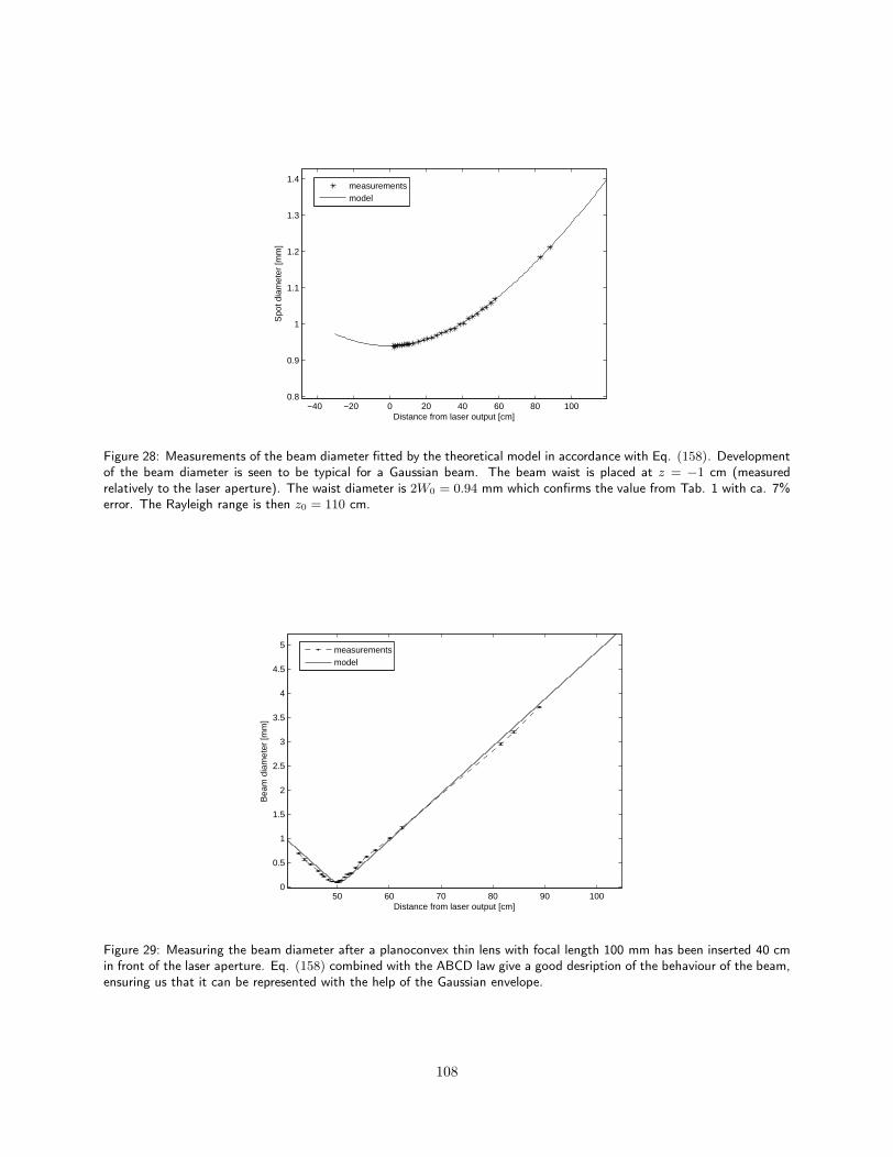
−40 −20 0 20 40 60 80 1000.8

0.9

1

1.1

1.2

1.3

1.4

Distance from laser output [cm]

Spo

t dia

met

er [m

m]

measurementsmodel

Figure 28: Measurements of the beam diameter fitted by the theoretical model in accordance with Eq. (158). Developmentof the beam diameter is seen to be typical for a Gaussian beam. The beam waist is placed at z = −1 cm (measuredrelatively to the laser aperture). The waist diameter is 2W0 = 0.94 mm which confirms the value from Tab. 1 with ca. 7%error. The Rayleigh range is then z0 = 110 cm.

50 60 70 80 90 1000

0.5

1

1.5

2

2.5

3

3.5

4

4.5

5

Distance from laser output [cm]

Bea

m d

iam

eter

[mm

]

measurementsmodel

Figure 29: Measuring the beam diameter after a planoconvex thin lens with focal length 100 mm has been inserted 40 cmin front of the laser aperture. Eq. (158) combined with the ABCD law give a good desription of the behaviour of the beam,ensuring us that it can be represented with the help of the Gaussian envelope.

108

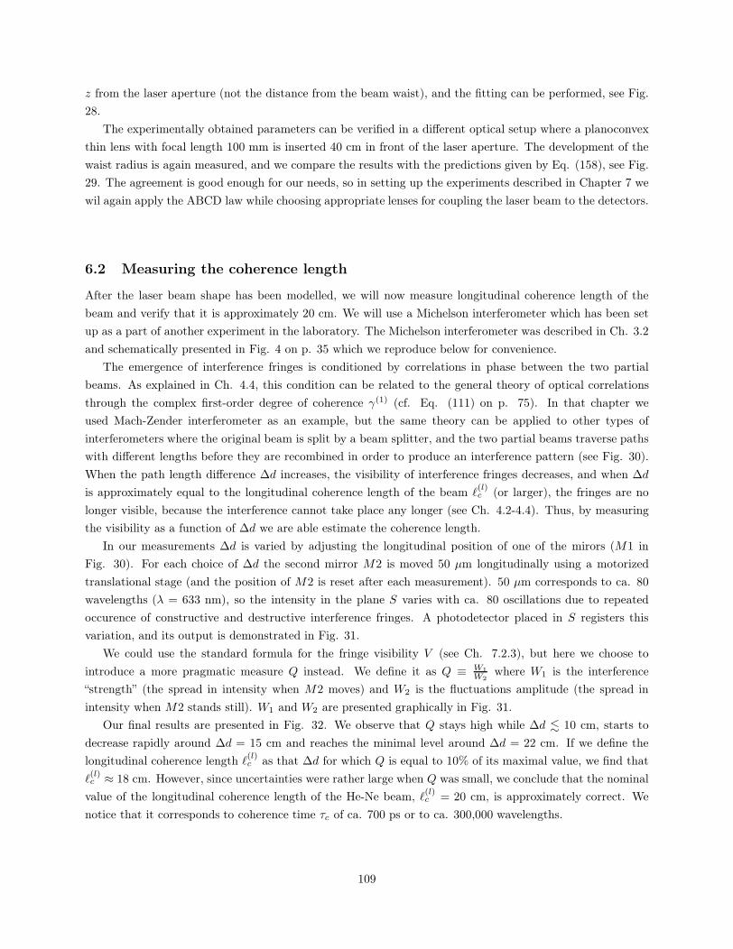
z from the laser aperture (not the distance from the beam waist), and the fitting can be performed, see Fig.

28.

The experimentally obtained parameters can be verified in a different optical setup where a planoconvex

thin lens with focal length 100 mm is inserted 40 cm in front of the laser aperture. The development of the

waist radius is again measured, and we compare the results with the predictions given by Eq. (158), see Fig.

29. The agreement is good enough for our needs, so in setting up the experiments described in Chapter 7 we

wil again apply the ABCD law while choosing appropriate lenses for coupling the laser beam to the detectors.

6.2 Measuring the coherence length

After the laser beam shape has been modelled, we will now measure longitudinal coherence length of the

beam and verify that it is approximately 20 cm. We will use a Michelson interferometer which has been set

up as a part of another experiment in the laboratory. The Michelson interferometer was described in Ch. 3.2

and schematically presented in Fig. 4 on p. 35 which we reproduce below for convenience.

The emergence of interference fringes is conditioned by correlations in phase between the two partial

beams. As explained in Ch. 4.4, this condition can be related to the general theory of optical correlations

through the complex first-order degree of coherence γ(1) (cf. Eq. (111) on p. 75). In that chapter we

used Mach-Zender interferometer as an example, but the same theory can be applied to other types of

interferometers where the original beam is split by a beam splitter, and the two partial beams traverse paths

with different lengths before they are recombined in order to produce an interference pattern (see Fig. 30).

When the path length difference ∆d increases, the visibility of interference fringes decreases, and when ∆d

is approximately equal to the longitudinal coherence length of the beam ℓ(l)c (or larger), the fringes are no

longer visible, because the interference cannot take place any longer (see Ch. 4.2-4.4). Thus, by measuring

the visibility as a function of ∆d we are able estimate the coherence length.

In our measurements ∆d is varied by adjusting the longitudinal position of one of the mirors (M1 in

Fig. 30). For each choice of ∆d the second mirror M2 is moved 50 µm longitudinally using a motorized

translational stage (and the position of M2 is reset after each measurement). 50 µm corresponds to ca. 80

wavelengths (λ = 633 nm), so the intensity in the plane S varies with ca. 80 oscillations due to repeated

occurence of constructive and destructive interference fringes. A photodetector placed in S registers this

variation, and its output is demonstrated in Fig. 31.

We could use the standard formula for the fringe visibility V (see Ch. 7.2.3), but here we choose to

introduce a more pragmatic measure Q instead. We define it as Q ≡ W1

W2where W1 is the interference

“strength” (the spread in intensity when M2 moves) and W2 is the fluctuations amplitude (the spread in

intensity when M2 stands still). W1 and W2 are presented graphically in Fig. 31.

Our final results are presented in Fig. 32. We observe that Q stays high while ∆d . 10 cm, starts to

decrease rapidly around ∆d = 15 cm and reaches the minimal level around ∆d = 22 cm. If we define the

longitudinal coherence length ℓ(l)c as that ∆d for which Q is equal to 10% of its maximal value, we find that

ℓ(l)c ≈ 18 cm. However, since uncertainties were rather large when Q was small, we conclude that the nominal

value of the longitudinal coherence length of the He-Ne beam, ℓ(l)c = 20 cm, is approximately correct. We

notice that it corresponds to coherence time τc of ca. 700 ps or to ca. 300,000 wavelengths.

109

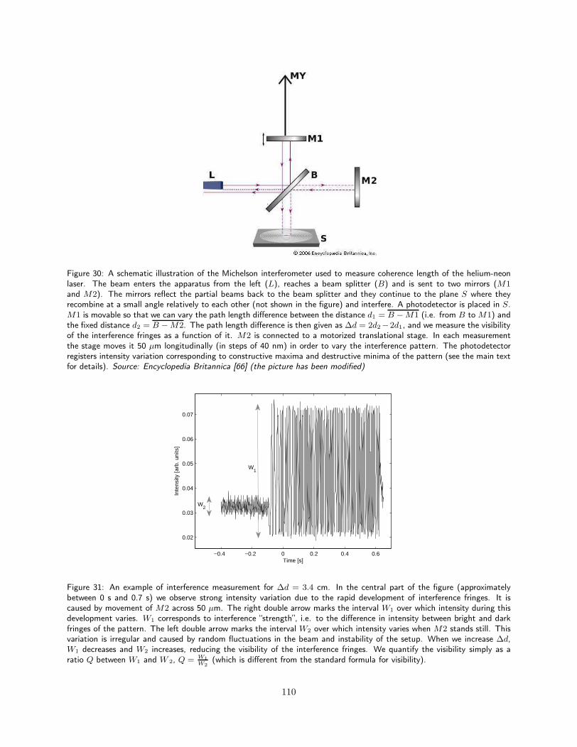
Figure 30: A schematic illustration of the Michelson interferometer used to measure coherence length of the helium-neonlaser. The beam enters the apparatus from the left (L), reaches a beam splitter (B) and is sent to two mirrors (M1and M2). The mirrors reflect the partial beams back to the beam splitter and they continue to the plane S where theyrecombine at a small angle relatively to each other (not shown in the figure) and interfere. A photodetector is placed in S.M1 is movable so that we can vary the path length difference between the distance d1 = B − M1 (i.e. from B to M1) andthe fixed distance d2 = B − M2. The path length difference is then given as ∆d = 2d2−2d1, and we measure the visibilityof the interference fringes as a function of it. M2 is connected to a motorized translational stage. In each measurementthe stage moves it 50 µm longitudinally (in steps of 40 nm) in order to vary the interference pattern. The photodetectorregisters intensity variation corresponding to constructive maxima and destructive minima of the pattern (see the main textfor details). Source: Encyclopedia Britannica [66] (the picture has been modified)

−0.4 −0.2 0 0.2 0.4 0.6

0.02

0.03

0.04

0.05

0.06

0.07

Time [s]

Inte

nsity

[arb

. uni

ts]

W2

W1

Figure 31: An example of interference measurement for ∆d = 3.4 cm. In the central part of the figure (approximatelybetween 0 s and 0.7 s) we observe strong intensity variation due to the rapid development of interference fringes. It iscaused by movement of M2 across 50 µm. The right double arrow marks the interval W1 over which intensity during thisdevelopment varies. W1 corresponds to interference “strength”, i.e. to the difference in intensity between bright and darkfringes of the pattern. The left double arrow marks the interval W2 over which intensity varies when M2 stands still. Thisvariation is irregular and caused by random fluctuations in the beam and instability of the setup. When we increase ∆d,W1 decreases and W2 increases, reducing the visibility of the interference fringes. We quantify the visibility simply as aratio Q between W1 and W 2, Q = W1

W2(which is different from the standard formula for visibility).

110

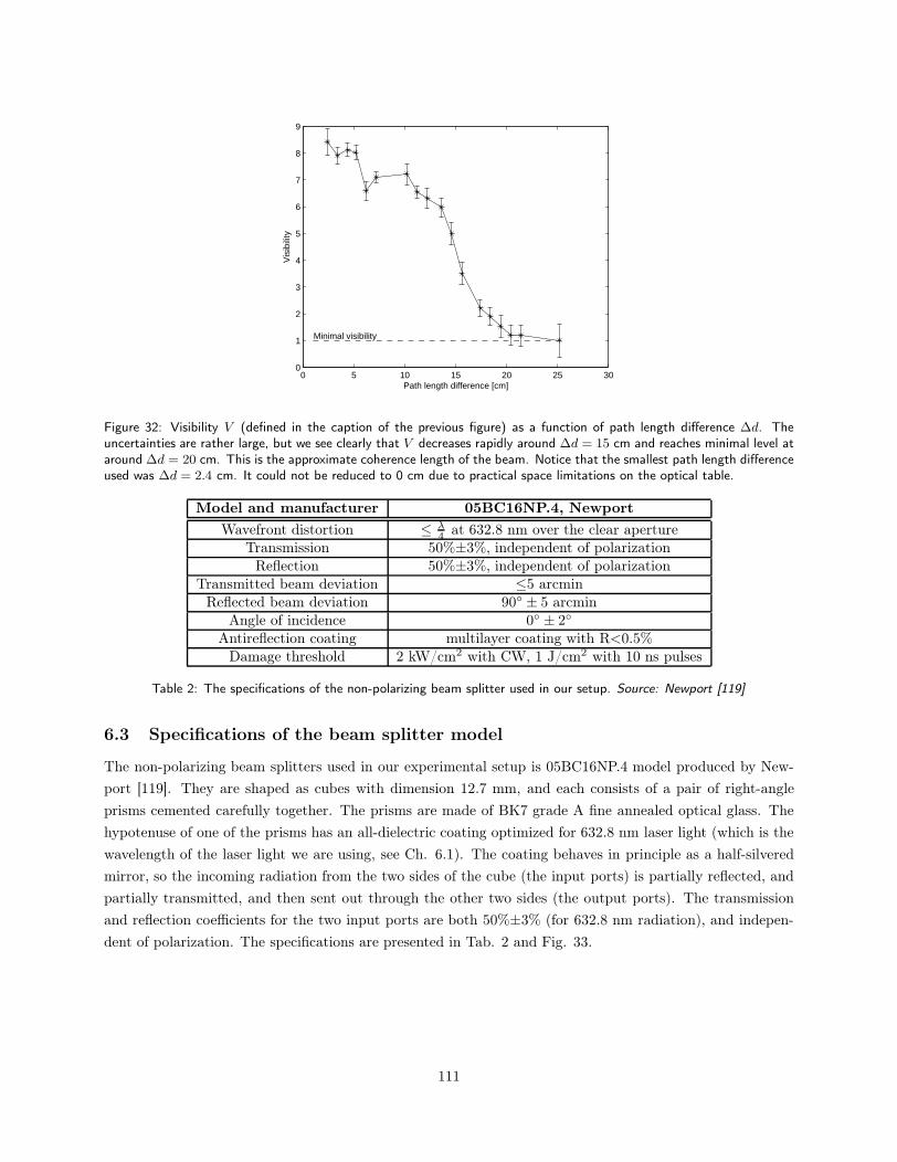
0 5 10 15 20 25 300

1

2

3

4

5

6

7

8

9

Path length difference [cm]

Vis

ibili

ty

Minimal visibility

Figure 32: Visibility V (defined in the caption of the previous figure) as a function of path length difference ∆d. Theuncertainties are rather large, but we see clearly that V decreases rapidly around ∆d = 15 cm and reaches minimal level ataround ∆d = 20 cm. This is the approximate coherence length of the beam. Notice that the smallest path length differenceused was ∆d = 2.4 cm. It could not be reduced to 0 cm due to practical space limitations on the optical table.

Model and manufacturer 05BC16NP.4, Newport

Wavefront distortion ≤ λ4 at 632.8 nm over the clear aperture

Transmission 50%±3%, independent of polarizationReflection 50%±3%, independent of polarization

Transmitted beam deviation ≤5 arcminReflected beam deviation 90 ± 5 arcmin

Angle of incidence 0 ± 2

Antireflection coating multilayer coating with R<0.5%Damage threshold 2 kW/cm2 with CW, 1 J/cm2 with 10 ns pulses

Table 2: The specifications of the non-polarizing beam splitter used in our setup. Source: Newport [119]

6.3 Specifications of the beam splitter model

The non-polarizing beam splitters used in our experimental setup is 05BC16NP.4 model produced by New-

port [119]. They are shaped as cubes with dimension 12.7 mm, and each consists of a pair of right-angle

prisms cemented carefully together. The prisms are made of BK7 grade A fine annealed optical glass. The

hypotenuse of one of the prisms has an all-dielectric coating optimized for 632.8 nm laser light (which is the

wavelength of the laser light we are using, see Ch. 6.1). The coating behaves in principle as a half-silvered

mirror, so the incoming radiation from the two sides of the cube (the input ports) is partially reflected, and

partially transmitted, and then sent out through the other two sides (the output ports). The transmission

and reflection coefficients for the two input ports are both 50%±3% (for 632.8 nm radiation), and indepen-

dent of polarization. The specifications are presented in Tab. 2 and Fig. 33.

111

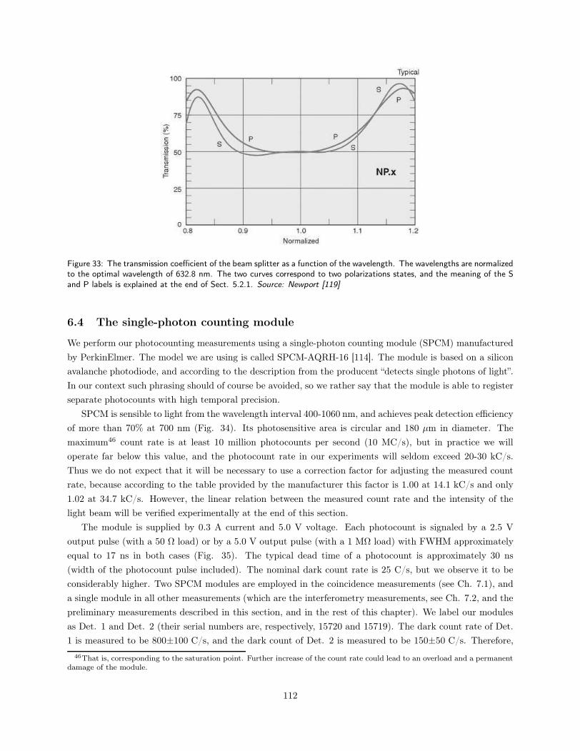
Figure 33: The transmission coefficient of the beam splitter as a function of the wavelength. The wavelengths are normalizedto the optimal wavelength of 632.8 nm. The two curves correspond to two polarizations states, and the meaning of the Sand P labels is explained at the end of Sect. 5.2.1. Source: Newport [119]

6.4 The single-photon counting module

We perform our photocounting measurements using a single-photon counting module (SPCM) manufactured

by PerkinElmer. The model we are using is called SPCM-AQRH-16 [114]. The module is based on a silicon

avalanche photodiode, and according to the description from the producent “detects single photons of light”.

In our context such phrasing should of course be avoided, so we rather say that the module is able to register

separate photocounts with high temporal precision.

SPCM is sensible to light from the wavelength interval 400-1060 nm, and achieves peak detection efficiency

of more than 70% at 700 nm (Fig. 34). Its photosensitive area is circular and 180 µm in diameter. The

maximum46 count rate is at least 10 million photocounts per second (10 MC/s), but in practice we will

operate far below this value, and the photocount rate in our experiments will seldom exceed 20-30 kC/s.

Thus we do not expect that it will be necessary to use a correction factor for adjusting the measured count

rate, because according to the table provided by the manufacturer this factor is 1.00 at 14.1 kC/s and only

1.02 at 34.7 kC/s. However, the linear relation between the measured count rate and the intensity of the

light beam will be verified experimentally at the end of this section.

The module is supplied by 0.3 A current and 5.0 V voltage. Each photocount is signaled by a 2.5 V

output pulse (with a 50 Ω load) or by a 5.0 V output pulse (with a 1 MΩ load) with FWHM approximately

equal to 17 ns in both cases (Fig. 35). The typical dead time of a photocount is approximately 30 ns

(width of the photocount pulse included). The nominal dark count rate is 25 C/s, but we observe it to be

considerably higher. Two SPCM modules are employed in the coincidence measurements (see Ch. 7.1), and

a single module in all other measurements (which are the interferometry measurements, see Ch. 7.2, and the

preliminary measurements described in this section, and in the rest of this chapter). We label our modules

as Det. 1 and Det. 2 (their serial numbers are, respectively, 15720 and 15719). The dark count rate of Det.

1 is measured to be 800±100 C/s, and the dark count of Det. 2 is measured to be 150±50 C/s. Therefore,

46That is, corresponding to the saturation point. Further increase of the count rate could lead to an overload and a permanentdamage of the module.

112

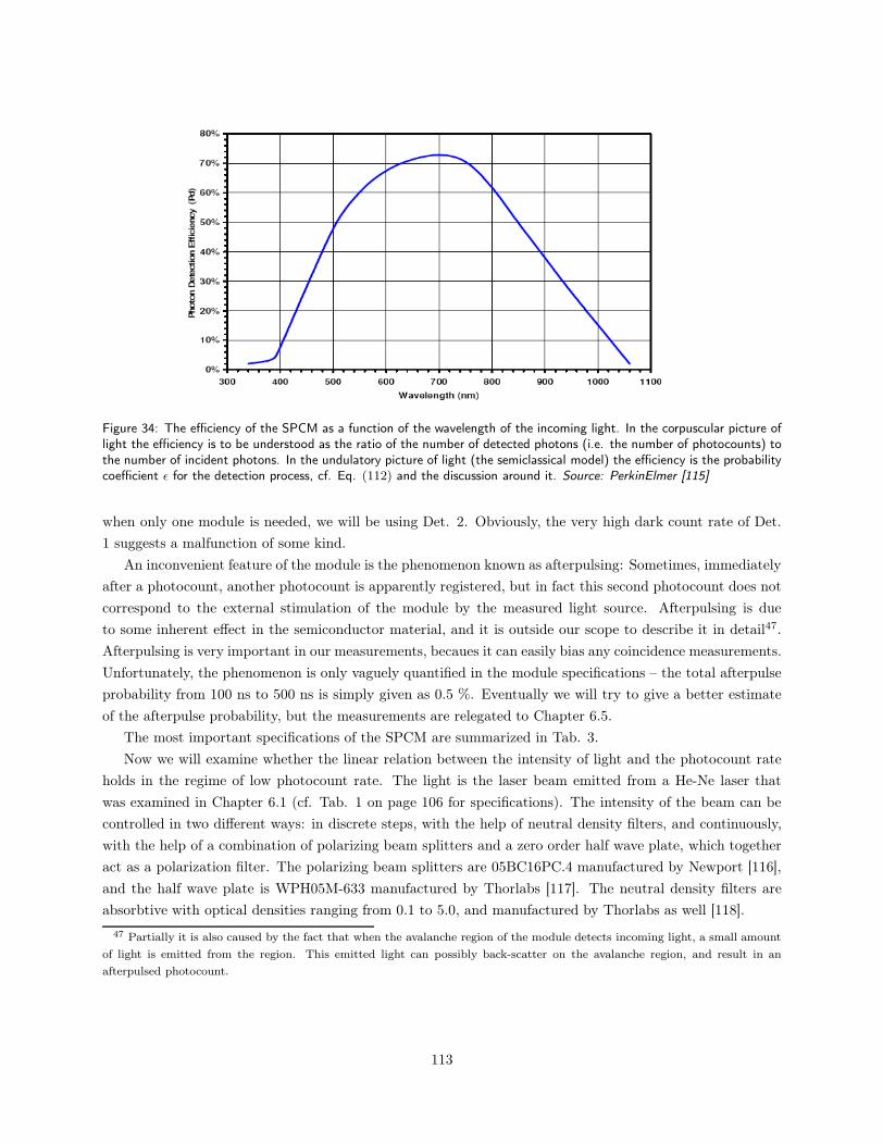
Figure 34: The efficiency of the SPCM as a function of the wavelength of the incoming light. In the corpuscular picture oflight the efficiency is to be understood as the ratio of the number of detected photons (i.e. the number of photocounts) tothe number of incident photons. In the undulatory picture of light (the semiclassical model) the efficiency is the probabilitycoefficient ǫ for the detection process, cf. Eq. (112) and the discussion around it. Source: PerkinElmer [115]

when only one module is needed, we will be using Det. 2. Obviously, the very high dark count rate of Det.

1 suggests a malfunction of some kind.

An inconvenient feature of the module is the phenomenon known as afterpulsing: Sometimes, immediately

after a photocount, another photocount is apparently registered, but in fact this second photocount does not

correspond to the external stimulation of the module by the measured light source. Afterpulsing is due

to some inherent effect in the semiconductor material, and it is outside our scope to describe it in detail47.

Afterpulsing is very important in our measurements, becaues it can easily bias any coincidence measurements.

Unfortunately, the phenomenon is only vaguely quantified in the module specifications – the total afterpulse

probability from 100 ns to 500 ns is simply given as 0.5 %. Eventually we will try to give a better estimate

of the afterpulse probability, but the measurements are relegated to Chapter 6.5.

The most important specifications of the SPCM are summarized in Tab. 3.

Now we will examine whether the linear relation between the intensity of light and the photocount rate

holds in the regime of low photocount rate. The light is the laser beam emitted from a He-Ne laser that

was examined in Chapter 6.1 (cf. Tab. 1 on page 106 for specifications). The intensity of the beam can be

controlled in two different ways: in discrete steps, with the help of neutral density filters, and continuously,

with the help of a combination of polarizing beam splitters and a zero order half wave plate, which together

act as a polarization filter. The polarizing beam splitters are 05BC16PC.4 manufactured by Newport [116],

and the half wave plate is WPH05M-633 manufactured by Thorlabs [117]. The neutral density filters are

absorbtive with optical densities ranging from 0.1 to 5.0, and manufactured by Thorlabs as well [118].

47 Partially it is also caused by the fact that when the avalanche region of the module detects incoming light, a small amount

of light is emitted from the region. This emitted light can possibly back-scatter on the avalanche region, and result in an

afterpulsed photocount.

113

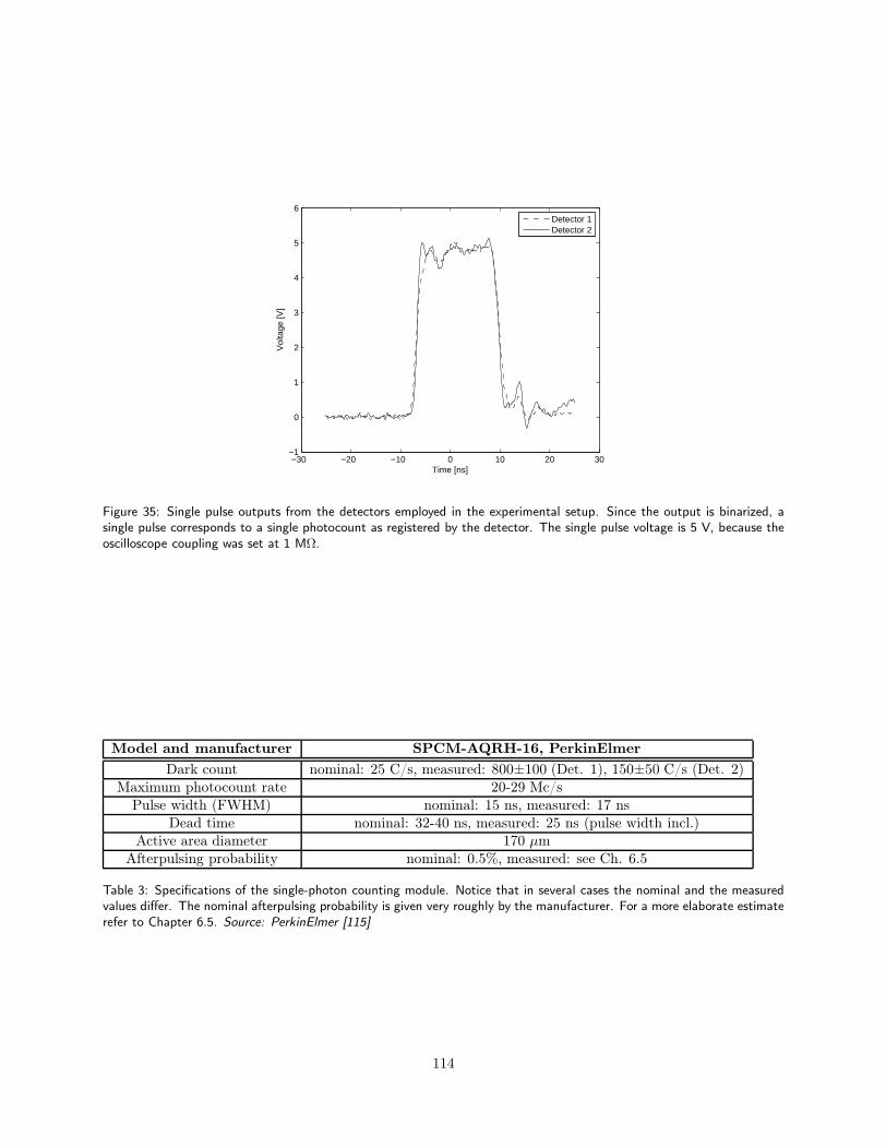
−30 −20 −10 0 10 20 30−1

0

1

2

3

4

5

6

Time [ns]

Vol

tage

[V]

Detector 1Detector 2

Figure 35: Single pulse outputs from the detectors employed in the experimental setup. Since the output is binarized, asingle pulse corresponds to a single photocount as registered by the detector. The single pulse voltage is 5 V, because theoscilloscope coupling was set at 1 MΩ.

Model and manufacturer SPCM-AQRH-16, PerkinElmer

Dark count nominal: 25 C/s, measured: 800±100 (Det. 1), 150±50 C/s (Det. 2)Maximum photocount rate 20-29 Mc/s

Pulse width (FWHM) nominal: 15 ns, measured: 17 nsDead time nominal: 32-40 ns, measured: 25 ns (pulse width incl.)

Active area diameter 170 µmAfterpulsing probability nominal: 0.5%, measured: see Ch. 6.5

Table 3: Specifications of the single-photon counting module. Notice that in several cases the nominal and the measuredvalues differ. The nominal afterpulsing probability is given very roughly by the manufacturer. For a more elaborate estimaterefer to Chapter 6.5. Source: PerkinElmer [115]

114

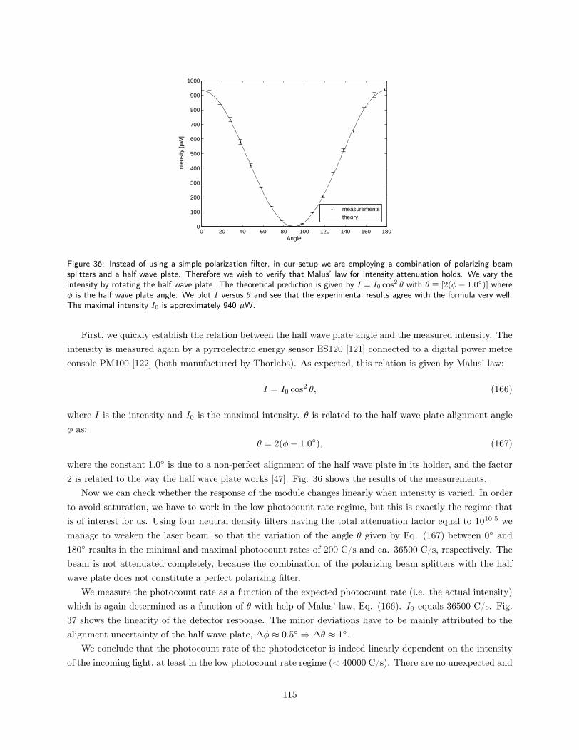
0 20 40 60 80 100 120 140 160 1800

100

200

300

400

500

600

700

800

900

1000

Angle

Inte

nsity

[µW

]

measurementstheory

Figure 36: Instead of using a simple polarization filter, in our setup we are employing a combination of polarizing beamsplitters and a half wave plate. Therefore we wish to verify that Malus’ law for intensity attenuation holds. We vary theintensity by rotating the half wave plate. The theoretical prediction is given by I = I0 cos2 θ with θ ≡ [2(φ − 1.0)] whereφ is the half wave plate angle. We plot I versus θ and see that the experimental results agree with the formula very well.The maximal intensity I0 is approximately 940 µW.

First, we quickly establish the relation between the half wave plate angle and the measured intensity. The

intensity is measured again by a pyrroelectric energy sensor ES120 [121] connected to a digital power metre

console PM100 [122] (both manufactured by Thorlabs). As expected, this relation is given by Malus’ law:

I = I0 cos2 θ, (166)

where I is the intensity and I0 is the maximal intensity. θ is related to the half wave plate alignment angle

φ as:

θ = 2(φ− 1.0), (167)

where the constant 1.0 is due to a non-perfect alignment of the half wave plate in its holder, and the factor

2 is related to the way the half wave plate works [47]. Fig. 36 shows the results of the measurements.

Now we can check whether the response of the module changes linearly when intensity is varied. In order

to avoid saturation, we have to work in the low photocount rate regime, but this is exactly the regime that

is of interest for us. Using four neutral density filters having the total attenuation factor equal to 1010.5 we

manage to weaken the laser beam, so that the variation of the angle θ given by Eq. (167) between 0 and

180 results in the minimal and maximal photocount rates of 200 C/s and ca. 36500 C/s, respectively. The

beam is not attenuated completely, because the combination of the polarizing beam splitters with the half

wave plate does not constitute a perfect polarizing filter.

We measure the photocount rate as a function of the expected photocount rate (i.e. the actual intensity)

which is again determined as a function of θ with help of Malus’ law, Eq. (166). I0 equals 36500 C/s. Fig.

37 shows the linearity of the detector response. The minor deviations have to be mainly attributed to the

alignment uncertainty of the half wave plate, ∆φ ≈ 0.5 ⇒ ∆θ ≈ 1.

We conclude that the photocount rate of the photodetector is indeed linearly dependent on the intensity

of the incoming light, at least in the low photocount rate regime (< 40000 C/s). There are no unexpected and

115

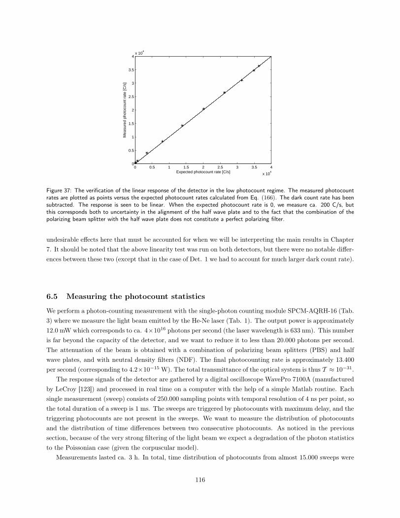
0 0.5 1 1.5 2 2.5 3 3.5 4

x 104

0

0.5

1

1.5

2

2.5

3

3.5

4x 10

4

Expected photocount rate [C/s]

Mea

sure

d ph

otoc

ount

rat

e [C

/s]

Figure 37: The verification of the linear response of the detector in the low photocount regime. The measured photocountrates are plotted as points versus the expected photocount rates calculated from Eq. (166). The dark count rate has beensubtracted. The response is seen to be linear. When the expected photocount rate is 0, we measure ca. 200 C/s, butthis corresponds both to uncertainty in the alignment of the half wave plate and to the fact that the combination of thepolarizing beam splitter with the half wave plate does not constitute a perfect polarizing filter.

undesirable effects here that must be accounted for when we will be interpreting the main results in Chapter

7. It should be noted that the above linearity test was run on both detectors, but there were no notable differ-

ences between these two (except that in the case of Det. 1 we had to account for much larger dark count rate).

6.5 Measuring the photocount statistics

We perform a photon-counting measurement with the single-photon counting module SPCM-AQRH-16 (Tab.

3) where we measure the light beam emitted by the He-Ne laser (Tab. 1). The output power is approximately

12.0 mW which corresponds to ca. 4×1016 photons per second (the laser wavelength is 633 nm). This number

is far beyond the capacity of the detector, and we want to reduce it to less than 20.000 photons per second.

The attenuation of the beam is obtained with a combination of polarizing beam splitters (PBS) and half

wave plates, and with neutral density filters (NDF). The final photocounting rate is approximately 13.400

per second (corresponding to 4.2×10−15 W). The total transmittance of the optical system is thus T ≈ 10−31.

The response signals of the detector are gathered by a digital oscilloscope WavePro 7100A (manufactured

by LeCroy [123]) and processed in real time on a computer with the help of a simple Matlab routine. Each

single measurement (sweep) consists of 250.000 sampling points with temporal resolution of 4 ns per point, so

the total duration of a sweep is 1 ms. The sweeps are triggered by photocounts with maximum delay, and the

triggering photocounts are not present in the sweeps. We want to measure the distribution of photocounts

and the distribution of time differences between two consecutive photocounts. As noticed in the previous

section, because of the very strong filtering of the light beam we expect a degradation of the photon statistics

to the Poissonian case (given the corpuscular model).

Measurements lasted ca. 3 h. In total, time distribution of photocounts from almost 15.000 sweeps were

116

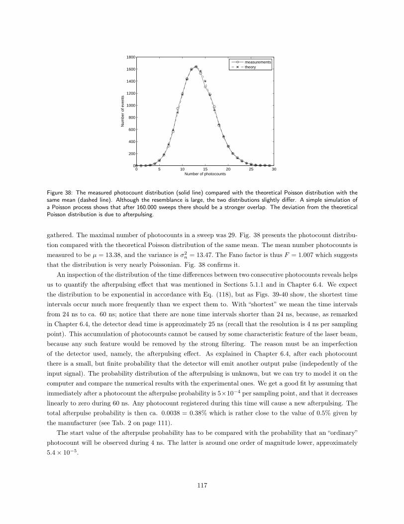
0 5 10 15 20 25 300

200

400

600

800

1000

1200

1400

1600

1800

Number of photocounts

Num

ber

of e

vent

s

measurementstheory

Figure 38: The measured photocount distribution (solid line) compared with the theoretical Poisson distribution with thesame mean (dashed line). Although the resemblance is large, the two distributions slightly differ. A simple simulation ofa Poisson process shows that after 160.000 sweeps there should be a stronger overlap. The deviation from the theoreticalPoisson distribution is due to afterpulsing.

gathered. The maximal number of photocounts in a sweep was 29. Fig. 38 presents the photocount distribu-

tion compared with the theoretical Poisson distribution of the same mean. The mean number photocounts is

measured to be µ = 13.38, and the variance is σ2n = 13.47. The Fano factor is thus F = 1.007 which suggests

that the distribution is very nearly Poissonian. Fig. 38 confirms it.

An inspection of the distribution of the time differences between two consecutive photocounts reveals helps

us to quantify the afterpulsing effect that was mentioned in Sections 5.1.1 and in Chapter 6.4. We expect

the distribution to be exponential in accordance with Eq. (118), but as Figs. 39-40 show, the shortest time

intervals occur much more frequently than we expect them to. With “shortest” we mean the time intervals

from 24 ns to ca. 60 ns; notice that there are none time intervals shorter than 24 ns, because, as remarked

in Chapter 6.4, the detector dead time is approximately 25 ns (recall that the resolution is 4 ns per sampling

point). This accumulation of photocounts cannot be caused by some characteristic feature of the laser beam,

because any such feature would be removed by the strong filtering. The reason must be an imperfection

of the detector used, namely, the afterpulsing effect. As explained in Chapter 6.4, after each photocount

there is a small, but finite probability that the detector will emit another output pulse (indepedently of the

input signal). The probability distribution of the afterpulsing is unknown, but we can try to model it on the

computer and compare the numerical results with the experimental ones. We get a good fit by assuming that

immediately after a photocount the afterpulse probability is 5×10−4 per sampling point, and that it decreases

linearly to zero during 60 ns. Any photocount registered during this time will cause a new afterpulsing. The

total afterpulse probability is then ca. 0.0038 = 0.38% which is rather close to the value of 0.5% given by

the manufacturer (see Tab. 2 on page 111).

The start value of the afterpulse probability has to be compared with the probability that an “ordinary”

photocount will be observed during 4 ns. The latter is around one order of magnitude lower, approximately

5.4 × 10−5.

117

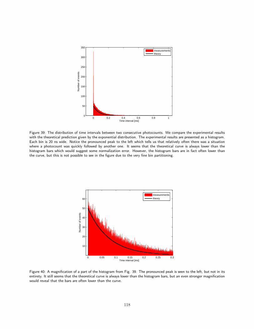
0 0.2 0.4 0.6 0.8 10

50

100

150

200

250

300

350

Time interval [ms]

Num

ber

of e

vent

s

measurementstheory

Figure 39: The distribution of time intervals between two consecutive photocounts. We compare the experimental resultswith the theoretical prediction given by the exponential distribution. The experimental results are presented as a histogram.Each bin is 20 ns wide. Notice the pronounced peak to the left which tells us that relatively often there was a situationwhere a photocount was quickly followed by another one. It seems that the theoretical curve is always lower than thehistogram bars which would suggest some normalization error. However, the histogram bars are in fact often lower thanthe curve, but this is not possible to see in the figure due to the very fine bin partitioning.

0 0.05 0.1 0.15 0.2 0.25 0.3

10

20

30

40

50

60

Time interval [ms]

Num

ber

of e

vent

s

measurementstheory

Figure 40: A magnification of a part of the histogram from Fig. 39. The pronounced peak is seen to the left, but not in itsentirety. It still seems that the theoretical curve is always lower than the histogram bars, but an even stronger magnificationwould reveal that the bars are often lower than the curve.

118

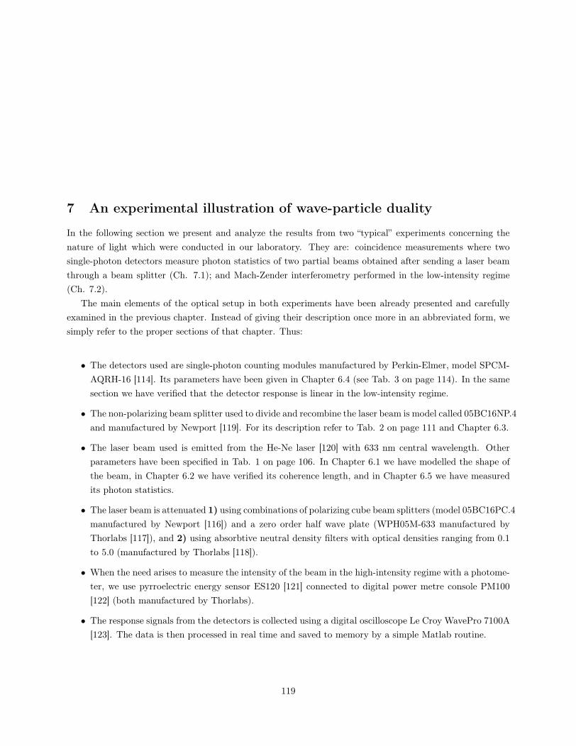
7 An experimental illustration of wave-particle duality

In the following section we present and analyze the results from two “typical” experiments concerning the

nature of light which were conducted in our laboratory. They are: coincidence measurements where two

single-photon detectors measure photon statistics of two partial beams obtained after sending a laser beam

through a beam splitter (Ch. 7.1); and Mach-Zender interferometry performed in the low-intensity regime

(Ch. 7.2).

The main elements of the optical setup in both experiments have been already presented and carefully

examined in the previous chapter. Instead of giving their description once more in an abbreviated form, we

simply refer to the proper sections of that chapter. Thus:

• The detectors used are single-photon counting modules manufactured by Perkin-Elmer, model SPCM-

AQRH-16 [114]. Its parameters have been given in Chapter 6.4 (see Tab. 3 on page 114). In the same

section we have verified that the detector response is linear in the low-intensity regime.

• The non-polarizing beam splitter used to divide and recombine the laser beam is model called 05BC16NP.4

and manufactured by Newport [119]. For its description refer to Tab. 2 on page 111 and Chapter 6.3.

• The laser beam used is emitted from the He-Ne laser [120] with 633 nm central wavelength. Other

parameters have been specified in Tab. 1 on page 106. In Chapter 6.1 we have modelled the shape of

the beam, in Chapter 6.2 we have verified its coherence length, and in Chapter 6.5 we have measured

its photon statistics.

• The laser beam is attenuated 1) using combinations of polarizing cube beam splitters (model 05BC16PC.4

manufactured by Newport [116]) and a zero order half wave plate (WPH05M-633 manufactured by

Thorlabs [117]), and 2) using absorbtive neutral density filters with optical densities ranging from 0.1

to 5.0 (manufactured by Thorlabs [118]).

• When the need arises to measure the intensity of the beam in the high-intensity regime with a photome-

ter, we use pyrroelectric energy sensor ES120 [121] connected to digital power metre console PM100

[122] (both manufactured by Thorlabs).

• The response signals from the detectors is collected using a digital oscilloscope Le Croy WavePro 7100A

[123]. The data is then processed in real time and saved to memory by a simple Matlab routine.

119

7.1 The coincidence measurements

7.1.1 Description

The coincidence measurements are performed in order to examine the corpuscular hypothesis which states

that the laser light consists of indivisible particles (called photons) of very small size (i.e. much smaller than

the central wavelength λ0 of the quasi-monochromatic laser beam). Due to the indivisibility, if we place two

single-photon detectors behind the output ports of a beam splitter, we expect that any such light particle

entering the beam splitter will be registered either by the first or by the second detector (given they are 100%

efficient), but not by both of them simultaneously.

The experiment can be considered as an alternative version of the experiment due to Grangier, Roger and

Aspect [89] where a cascade light source was employed (see Ch. 3.5). There are following differences between

these two:

1. The light source employed by us is a laser beam with coherence length of 20 cm while Grangier et al.

used a radiative cascade originating from excited calcium atoms. The coherence length of the cascade

was not explicitly given, but it is assumed that it was much shorter than 20 cm.

2. Our experiment is not triggered by means of correlated emission, so background photocounts might

present a problem. However, since the dark count rates of detectors are very low, the results should

not be biased (this assumption will be confirmed during our analysis).

3. We analyze the results by comparing them with the results of numerical models (see Sect. 7.1.4), while

Grangier et al. made an analytical (but simplified) comparison with the semiclassical and the fully

quantum-mechanical models.

We stress that we do not set out to disprove the results of Grangier et al. We simply want to conduct a

similar experiment in order to illustrate how the the wave-particle duality of light may be discussed in the

context of coincidence measurements performed on a coherent laser beam which is a “classical” light source

as opposed to the light source employed by Grangier et al.

7.1.2 Setup and discussion of photocount rates

The experimental setup is presented in Fig. 41. The attenuated beam reaches the non-polarizing beam

splitter and the two partial beams continue to the detectors. The optical path length between the laser

aperture and the beam splitter is 1.49 m; the optical path length between the beam splitter and Det. 1 (Det.

2) is 55 cm (98 cm). Division by the speed of light c yields the time needed for the emitted laser light to reach

the detectors: it is 6.8 ns for Det. 1 and 8.2 ns for Det. 2. The difference between these two is negligible,

because it is smaller than the time resolution employed in our setup (see Sect. 7.1.3). The partial beams

are focused into the detector apertures using two convex thin lenses with focal lengths 100 mm. The beam

radius W (see Eq. (158) on p. 102) at the positions of the apertures can be calculated as 45.0± 5.0 µm (for

120

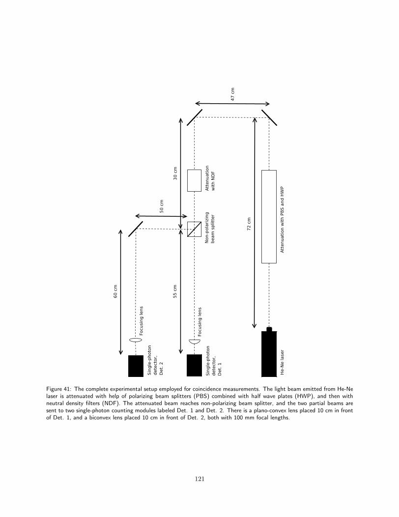
Figure 41: The complete experimental setup employed for coincidence measurements. The light beam emitted from He-Nelaser is attenuated with help of polarizing beam splitters (PBS) combined with half wave plates (HWP), and then withneutral density filters (NDF). The attenuated beam reaches non-polarizing beam splitter, and the two partial beams aresent to two single-photon counting modules labeled Det. 1 and Det. 2. There is a plano-convex lens placed 10 cm in frontof Det. 1, and a biconvex lens placed 10 cm in front of Det. 2, both with 100 mm focal lengths.

121

both beams) which is well below the active area radius of apertures (85 µm, see Tab. 3 on p. 114).

During the measurements the mean total photocount rate of Det. 1 was N1,tot = 14700 C/s (counts per

second48), and the mean total photocount rate of Det. 2 was N2,tot = 7800 C/s. The total background

photocount rate49 of Det. 1 is N1,BG = 850 C/s, and the total background photocount rate of Det. 2 is

N2,BG = 200 C/s. Thus the photocount rate due to the spli laser beam alone is, for Det. 1:

N1,las = N1,tot −N1,BG = 13850 C/s,

and, for Det. 2:

N2,las = N2,tot −N2,BG = 7600 C/s.

We would expect N1 and N2 to be approximately equal, since the original beam is split using a 50:50

beam splitter. The splitting, however, might be non-perfect due to misalignment of the beam splitter. In

order to check this, we measure the intensity with a photometer directly in front of Det. 1 and Det. 2.

We find then that the intensity of the split beam going to Det. 2 equals 88% of the intensity of the split

beam going to Det. 1. Nonetheless it does not explain that N1 is almost twice as large as N2, so we have to

conclude that the effectivity of Det. 2 is considerably smaller than the effectivity of Det. 1.

The intensity of the laser beam right after emission is 12.0 mW. After attenuating the beam with polarizing

beam splitters and half wave plates, its intensity is reduced to 925 µW. The total attenuation due to neutral

density filters is 10−10.79, so the intensity is reduced further to 0.015 pW. It is impossible to measure such

extremely low intensity directly with a photometer, so it has been inferred from the optical densities of the

filters.

Since the (central) wavelength of the light employed is 633 nm, formula E = hf = hcλ yielding single

photon energy tells us that 0.015 pW corresponds to approximately 50.000 photons per second (if we work

within the corpuscular model). We then find that Det. 1 should receive ca. 26500 photons per second, and

that Det. 2 should receive ca. 23500 photon per second. Given the Poissonian distribution of the photons,

the mean time interval between two consecutive photons reaching Det. 1 or Det. 2 is approximately 40 µs.

This is much larger than the time needed for the laser light to reach detectors after being emitted from the

laser aperture (which is less than 10 ns, see figures quoted above), so we can assume that at any time there

is maximally one photon present in the apparatus.

At 633 nm central wavelength the nominal quantum efficiency of the detectors is ǫN,1 = ǫN,2 = 70% (cf.

Fig. 34 on page 113). Thus we expect that Det. 1 should measure 18600 C/s and that Det. 2 should measure

16500 C/s (from the partial beams alone). These numbers have to be confronted with N1,las and N2,las. We

estimate that the efficiency of Det. 1 is in fact ǫ1 = 51%, and that the efficiency of Det. 2 is ǫ2 = 32%. These

ratios are low compared to the nominal quantum efficiency. However, we have to remember that the coupling

of the partial beams into the detector apertures is not necessarily perfect. Furthermore, it is possible that

the beam intensity after attenuation is lower than 0.015 pW, since the optical densities of the neutral density

filters have been measured and calculated in the high-intensity regime, and in the low-intensity regime some

additional effects could occur.

The suspected low efficiencies will not, however, pose a real problem for obtaining good statistics, since

48Uncertainty for all photocount rates is estimated as ±100 C/s49With the total background photocount rate we mean the dark count rate plus the photocount rate due to the stray light in

the laboratory. The measurements of the laser beam are not performed in total darkness, because of several LED’s belongingto different laboratory devices. We keep in mind that the dark count rate of Det. 1 is considerably higher than that of Det. 2(cf. Tab. 3 on page 114).

122

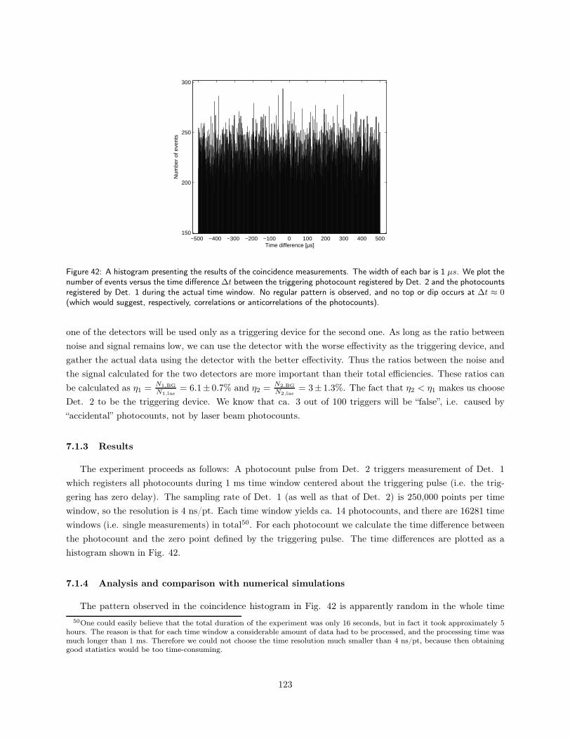
−500 −400 −300 −200 −100 0 100 200 300 400 500150

200

250

300

Time difference [µs]

Num

ber

of e

vent

s

Figure 42: A histogram presenting the results of the coincidence measurements. The width of each bar is 1 µs. We plot thenumber of events versus the time difference ∆t between the triggering photocount registered by Det. 2 and the photocountsregistered by Det. 1 during the actual time window. No regular pattern is observed, and no top or dip occurs at ∆t ≈ 0(which would suggest, respectively, correlations or anticorrelations of the photocounts).

one of the detectors will be used only as a triggering device for the second one. As long as the ratio between

noise and signal remains low, we can use the detector with the worse effectivity as the triggering device, and

gather the actual data using the detector with the better effectivity. Thus the ratios between the noise and

the signal calculated for the two detectors are more important than their total efficiencies. These ratios can

be calculated as η1 =N1,BG

N1,las= 6.1± 0.7% and η2 =

N2,BG

N2,las= 3± 1.3%. The fact that η2 < η1 makes us choose

Det. 2 to be the triggering device. We know that ca. 3 out of 100 triggers will be “false”, i.e. caused by

“accidental” photocounts, not by laser beam photocounts.

7.1.3 Results

The experiment proceeds as follows: A photocount pulse from Det. 2 triggers measurement of Det. 1

which registers all photocounts during 1 ms time window centered about the triggering pulse (i.e. the trig-

gering has zero delay). The sampling rate of Det. 1 (as well as that of Det. 2) is 250,000 points per time

window, so the resolution is 4 ns/pt. Each time window yields ca. 14 photocounts, and there are 16281 time

windows (i.e. single measurements) in total50. For each photocount we calculate the time difference between

the photocount and the zero point defined by the triggering pulse. The time differences are plotted as a

histogram shown in Fig. 42.

7.1.4 Analysis and comparison with numerical simulations

The pattern observed in the coincidence histogram in Fig. 42 is apparently random in the whole time

50One could easily believe that the total duration of the experiment was only 16 seconds, but in fact it took approximately 5hours. The reason is that for each time window a considerable amount of data had to be processed, and the processing time wasmuch longer than 1 ms. Therefore we could not choose the time resolution much smaller than 4 ns/pt, because then obtaininggood statistics would be too time-consuming.

123

interval, and its Fourier analysis does not reveal any regularities. More importantly, there is no dip around the

region where ∆t ≈ 0. The occurence of such a dip would serve as a proof that at the moment of triggering

Det. 2 with a photocount Det. 1 registers photocounts only seldom. This would again suggest that the

photons going through the beam splitter are indeed indivisible, and, furthermore, that they do not travel in

clusters (or, if they do, that the clusters are not being divided by the beam splitter, but rather sent along

one of the optical paths in their entireties, see also Ch. 9.1).

Two issues must be considered. Firstly, we ask to what degree the presence of dark counts, background

photocounts and afterpulses affect the coincidence statistics. We know that the rate of all these effects

combined is small compared to the photocount rate associated with the partial beams of the laser. Nonetheless

we have to admit the possibility that in the case of coincidence measurements some bias will be introduced

due to these “accidental” photocounts.

Secondly, we know from the photocount statistics measurements described in Chapter 6.5 that the dis-

tribution of the laser photocounts in time is Poissonian. As explained in Section 5.1.3, even if the original

emission of light had been characterized by sub-Poissonian or super-Poissonian distribution of photons (within

the corpuscular model), this distribution would be reduced to the Poissonian one anyway because of the very

strong attenuation of the beam. Thus we have to find out what coincidence histogram is expected in the case

of Poissonian distribution.

In order to answer the above questions simultaneously and in an illustrative way we have written a

Matlab program which simulates the coincidence measurements (the code is included in Appendix D). The

program takes into account all features of the detection process hitherto discussed (dark and background

counts, afterpulsing, detector dead time). Furthermore it allows us to manipulate freely the parameters

describing the original distribution of the photons, the beam splitting process and the detection process (i.e.

the conversion of photons to photocounts).

The program can be easily modified in order to accommodate different models of light. Thus we will not

only see what coincidence histogram should be experimentally expected when we picture light as Poisson-

distributed, indivisible photons, but also what histograms should result from other models. The scenarios

considered are:

1. A stream of indivisible photons that are well-separated in space

(a) a completely regular stream

(b) a Poisson-distributed stream

(c) a Poisson-distributed stream with weak bunching effect

(d) a Poisson-distributed stream with weak antibunching effect

2. A stream of divisible, narrow wave packets that are well-separated in space

(a) a Poisson-distributed stream

(b) a Poisson-distributed stream with weak bunching effect

(c) a Poisson-distributed stream with weak antibunching effect

3. Continuous radiation

In the following the parameters corresponding to dark and background counts, afterpulsing, detector dead

time are chosen to be the same as in our setup. The temporal resolution and length of each realization are

also identical to the ones in the actual experiment.

124

We begin by examining the implications of model 1a. This is an ideal situation, but it helps us to establish

that our numerical routines work properly. The coincidence histogram is presented in Fig. 43. The regular

stream of photons results in no correlations around zero time difference, ∆t ≈ 0, but very strong correlations

start to show at |∆t| = 20 µs and they repeat themselves with 20 µs interval which of course corresponds to

the time interval between two consecutive photons in the original beam. The uniformly distributed dark and

background counts are clearly visible in the bottom of the histogram.

The simulation results for models 1b and 1c are presented, respectively, in Figs. 44 and 45. Histogram

in Fig. 44 resembles our original histogram created from the experimental data. The variation of the number

of events as a function of time difference is apparently random in the whole interval. No top or dip occurs

at ∆t ≈ 0, and Fourier analysis does not reveal any regularities. Histogram in Fig. 45 shows that in the

case of bunched51 photons one should expect a top at ∆t ≈ 0. This top reflects the frequently occuring

situation where two photons, originally located close to each other, pass through the beam splitter and where

one of them is sent to Det. 2 and acts as a trigger, while the second of them is (almost) coincidentally

registered by Det. 1. The simulations results for model 1c is not shown explicitly, but commented upon

in the caption of Fig. 45 – in the case of weakly antibunched photons we would simply obtain a dip at

∆t ≈ 0, for converse reasons. We remember that in our setup the beam has been strongly attenuated, so in

the standard corpuscular model only the Poisson distribution is possible, but it is instructive to examine all

three scenarios.

We now change the basic hypothesis by assuming that the beam splitter is able to split any single photon

in two parts. In other words, instead of photons we work now with wave packets that are well-separated

in space and of very short duration52. The modelled beam splitter divides now each wave packet in two

parts of approximately equal intensity (some stochastic variation is allowed), the parts are sent on to the

detectors, and the detection probability (i.e. the photocount probability) is proportional to the intensity of

the incoming signal. The results for model 2b (with a weak bunching of wave packets) are shown explicitly

in Fig. 46. We observe a very sharp peak at ∆t = 0 corresponding to the coincidences caused by the splitting

of the single wave packets in the beam splitter. This central coincidental bar is surrounded by a much smaller

top which is reminiscent of the top from Fig. 45. Of course, this top is due to bunching of wave packets. In

models 2a and 2c we would see (the histograms are not shown), respectively, no such top and a dip instead

of a top. However, the central coincidental peak is present in all cases, and no such peak has been observed

in our experimental results.

Finally we consider model 3 where light is modelled as strongly attenuated, but nonetheless continuous

radiative field. The fundamental frequency of this field, corresponding to 633 nm, is 4.74 × 1014 Hz which

yields an oscillation period of 2.11×10−15 s. This is several orders of magnitude less than resolution capability

of the detector (which is around 1 ps [114]), so as far as this capability is concerned, the intensity of the

field is constant. In addition we have to consider coherence time. However, longitudinal coherence length

of the beam is only 20 cm, so coherence time is only 700 ps. Since our time resolution (4 ns) is almost six

times longer than the coherence time, we will be unable to measure any correlations on the coherence time

scale (see Chapter 4) and the resulting coincidence histogram will be random and bereft of any features, as

51The photon occurence probability in a time step is originally 0.0002 . To simulate bunching, this probability increases to0.00035 immediately after a photon has occured, and then decreases linearly back to 0.0002 during time interval of 1000 timesteps (4 µs in our models). The antibunching is simulated in a similar way. Notice that the modelled beam splitter still processesphotons indepedently, even if they are bunched or antibunched.

52With “very short duration” we mean that their temporal length is much shorter than dead time of the detectors, so onewave packet may give rise to maximally one photocount.

125

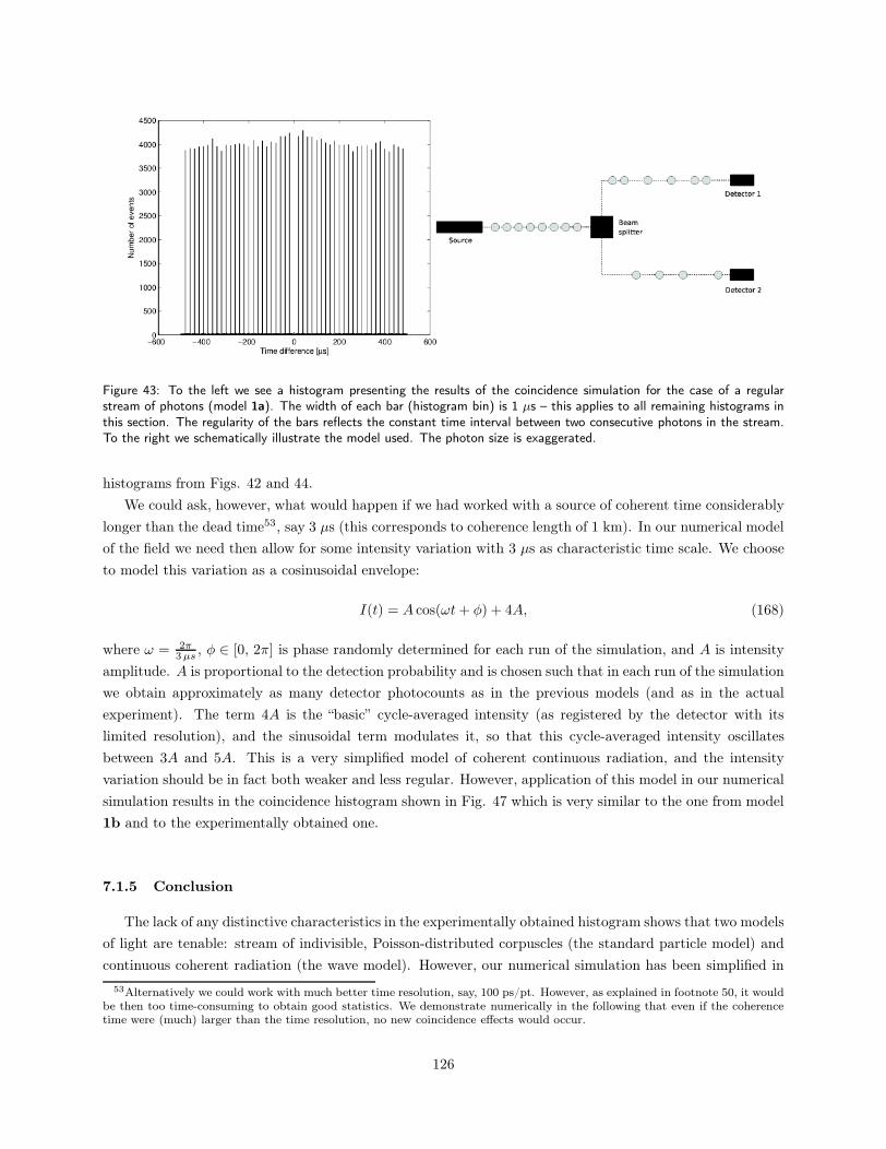
Figure 43: To the left we see a histogram presenting the results of the coincidence simulation for the case of a regularstream of photons (model 1a). The width of each bar (histogram bin) is 1 µs – this applies to all remaining histograms inthis section. The regularity of the bars reflects the constant time interval between two consecutive photons in the stream.To the right we schematically illustrate the model used. The photon size is exaggerated.

histograms from Figs. 42 and 44.

We could ask, however, what would happen if we had worked with a source of coherent time considerably

longer than the dead time53, say 3 µs (this corresponds to coherence length of 1 km). In our numerical model

of the field we need then allow for some intensity variation with 3 µs as characteristic time scale. We choose

to model this variation as a cosinusoidal envelope:

I(t) = A cos(ωt+ φ) + 4A, (168)

where ω = 2π3 µs , φ ∈ [0, 2π] is phase randomly determined for each run of the simulation, and A is intensity

amplitude. A is proportional to the detection probability and is chosen such that in each run of the simulation

we obtain approximately as many detector photocounts as in the previous models (and as in the actual

experiment). The term 4A is the “basic” cycle-averaged intensity (as registered by the detector with its

limited resolution), and the sinusoidal term modulates it, so that this cycle-averaged intensity oscillates

between 3A and 5A. This is a very simplified model of coherent continuous radiation, and the intensity

variation should be in fact both weaker and less regular. However, application of this model in our numerical

simulation results in the coincidence histogram shown in Fig. 47 which is very similar to the one from model

1b and to the experimentally obtained one.

7.1.5 Conclusion

The lack of any distinctive characteristics in the experimentally obtained histogram shows that two models

of light are tenable: stream of indivisible, Poisson-distributed corpuscles (the standard particle model) and

continuous coherent radiation (the wave model). However, our numerical simulation has been simplified in

53Alternatively we could work with much better time resolution, say, 100 ps/pt. However, as explained in footnote 50, it wouldbe then too time-consuming to obtain good statistics. We demonstrate numerically in the following that even if the coherencetime were (much) larger than the time resolution, no new coincidence effects would occur.

126

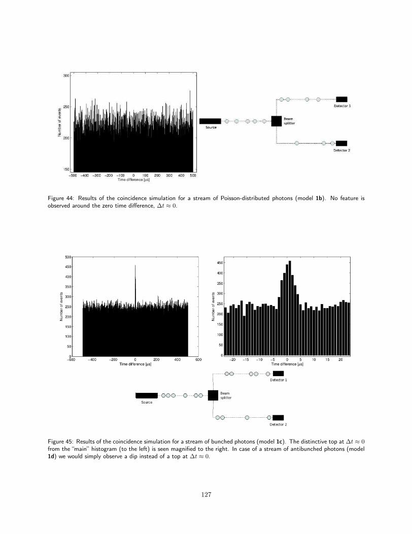
Figure 44: Results of the coincidence simulation for a stream of Poisson-distributed photons (model 1b). No feature isobserved around the zero time difference, ∆t ≈ 0.

Figure 45: Results of the coincidence simulation for a stream of bunched photons (model 1c). The distinctive top at ∆t ≈ 0from the “main” histogram (to the left) is seen magnified to the right. In case of a stream of antibunched photons (model1d) we would simply observe a dip instead of a top at ∆t ≈ 0.

127

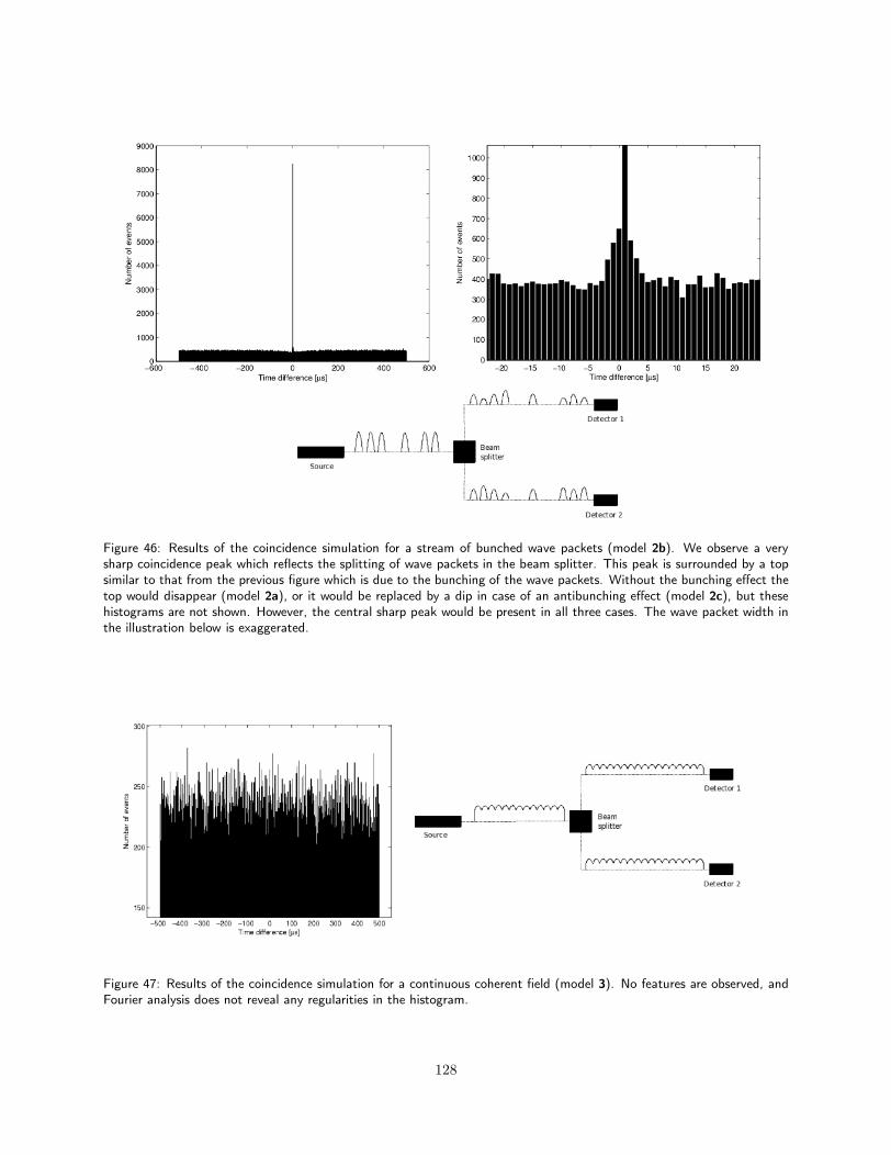
Figure 46: Results of the coincidence simulation for a stream of bunched wave packets (model 2b). We observe a verysharp coincidence peak which reflects the splitting of wave packets in the beam splitter. This peak is surrounded by a topsimilar to that from the previous figure which is due to the bunching of the wave packets. Without the bunching effect thetop would disappear (model 2a), or it would be replaced by a dip in case of an antibunching effect (model 2c), but thesehistograms are not shown. However, the central sharp peak would be present in all three cases. The wave packet width inthe illustration below is exaggerated.

Figure 47: Results of the coincidence simulation for a continuous coherent field (model 3). No features are observed, andFourier analysis does not reveal any regularities in the histogram.

128

some respects and has built on specific assumptions in others, so at least two reservations must be immediately

made:

1. Since we work in the low-intensity regime, we are not guaranteed that the beam splitter exhibits

standard behaviour. It is conceivable that model 2a could be corroborated if we had included in the

simulation some additional effects that might be associated with the functioning of the beam splitter

at very low intensities. This claim should be compared with what have been said about shortcomings

of the standard beam splitter models in Chapter 5.2.3. As the program code from Appendix D shows,

in our simulation the beam splitter model used is very simple indeed.

2. Our model of coherent radiation is admittedly simplistic. However, its simplicity may be perceived

as an asset, because it demonstrates that even if the intensity envelope would be as regular as in Eq.

(168) (and the intensity variation as strong), the resulting coincidence histogram would nonetheless be

similar to the one we had obtained in the experiment. A more careful modelling of continuous coherence

radiation would introduce more random elements into the radiative pattern and lessen its variation, so

it is difficult to see how these elements could lead to a different histogram (in the sense of possessing

coincidental or anticoincidental features).

We conclude that the coincidence measurements performed on a strongly attenuated coherent laser beam

does not demonstrate its corpuscular properties unambiguously, because the same results can be obtained

on the basis of classical model. This is in accordance with what have been said in Chapter 4.3 and Section

5.1.4 about, respectively, the classical description of coherence and the semiclassical model of photodetection.

Thus our results are by no means novel, but simply serve as an experimental and numerical illustration of

the theory. As remarked in Sect. 7.1.1, presenting such an illustration was our goal in this chapter.

7.2 The Mach-Zender interferometry

7.2.1 Description

We perform a Mach-Zender interferometry experiment with a single-photon counting module in order to

confirm the occurence of interference fringes in the low-intensity regime. The crucial connection between

the interference fringes and the wave aspect of electromagnetic radiation has been elaborated on in Chapter

3.2, while in Chapter 4.4 we have presented the Mach-Zender interferometry in the framework of optical

correlations theory. The latter, however, will not be employed here.

7.2.2 Setup

The experimental setup is shown in Fig. 48. Up until the first non-polarizing beam splitter it is identical

to the one employed in the coincidence measurements and depicted in Fig. 41. The split beam is then sent

along two different optical paths to the second non-polarizing beam splitter where the partial beams are

recombined. The length of the Path 1 (refer to Fig. 48) is 81 cm, the length of the Path 2 is 90 cm. The

129

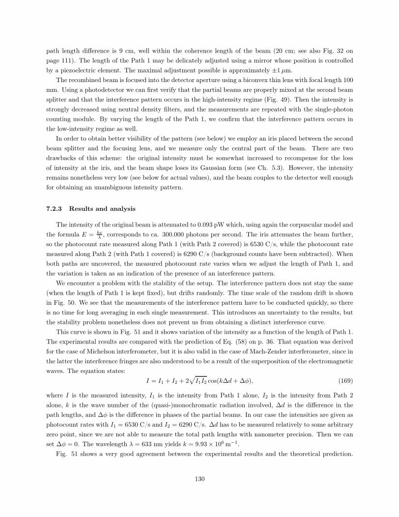
path length difference is 9 cm, well within the coherence length of the beam (20 cm; see also Fig. 32 on

page 111). The length of the Path 1 may be delicately adjusted using a mirror whose position is controlled

by a piezoelectric element. The maximal adjustment possible is approximately ±1µm.

The recombined beam is focused into the detector aperture using a biconvex thin lens with focal length 100

mm. Using a photodetector we can first verify that the partial beams are properly mixed at the second beam

splitter and that the interference pattern occurs in the high-intensity regime (Fig. 49). Then the intensity is

strongly decreased using neutral density filters, and the measurements are repeated with the single-photon

counting module. By varying the length of the Path 1, we confirm that the interference pattern occurs in

the low-intensity regime as well.

In order to obtain better visibility of the pattern (see below) we employ an iris placed between the second

beam splitter and the focusing lens, and we measure only the central part of the beam. There are two

drawbacks of this scheme: the original intensity must be somewhat increased to recompense for the loss

of intensity at the iris, and the beam shape loses its Gaussian form (see Ch. 5.3). However, the intensity

remains nonetheless very low (see below for actual values), and the beam couples to the detector well enough

for obtaining an unambiguous intensity pattern.

7.2.3 Results and analysis

The intensity of the original beam is attenuated to 0.093 pW which, using again the corpuscular model and

the formula E = hcλ , corresponds to ca. 300.000 photons per second. The iris attenuates the beam further,

so the photocount rate measured along Path 1 (with Path 2 covered) is 6530 C/s, while the photocount rate

measured along Path 2 (with Path 1 covered) is 6290 C/s (background counts have been subtracted). When

both paths are uncovered, the measured photocount rate varies when we adjust the length of Path 1, and

the variation is taken as an indication of the presence of an interference pattern.

We encounter a problem with the stability of the setup. The interference pattern does not stay the same

(when the length of Path 1 is kept fixed), but drifts randomly. The time scale of the random drift is shown

in Fig. 50. We see that the measurements of the interference pattern have to be conducted quickly, so there

is no time for long averaging in each single measurement. This introduces an uncertainty to the results, but

the stability problem nonetheless does not prevent us from obtaining a distinct interference curve.

This curve is shown in Fig. 51 and it shows variation of the intensity as a function of the length of Path 1.

The experimental results are compared with the prediction of Eq. (58) on p. 36. That equation was derived

for the case of Michelson interferometer, but it is also valid in the case of Mach-Zender interferometer, since in

the latter the interference fringes are also understood to be a result of the superposition of the electromagnetic

waves. The equation states:

I = I1 + I2 + 2√

I1I2 cos(k∆d+ ∆φ), (169)

where I is the measured intensity, I1 is the intensity from Path 1 alone, I2 is the intensity from Path 2

alone, k is the wave number of the (quasi-)monochromatic radiation involved, ∆d is the difference in the

path lengths, and ∆φ is the difference in phases of the partial beams. In our case the intensities are given as

photocount rates with I1 = 6530 C/s and I2 = 6290 C/s. ∆d has to be measured relatively to some arbitrary

zero point, since we are not able to measure the total path lengths with nanometer precision. Then we can

set ∆φ = 0. The wavelength λ = 633 nm yields k = 9.93 × 106 m−1.

Fig. 51 shows a very good agreement between the experimental results and the theoretical prediction.

130

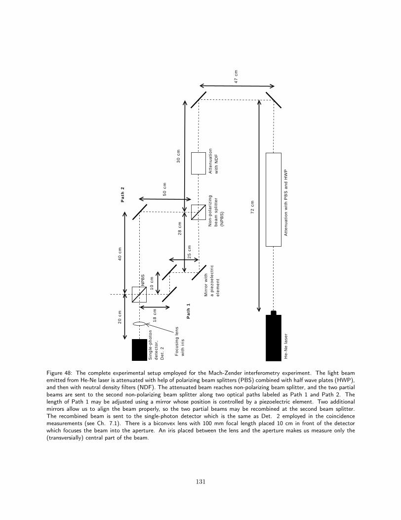
He

-Ne

la

ser

Att

en

ua

tio

n w

ith

PB

S a

nd

HW

PAtt

en

ua

tio

nw

ith

ND

F

No

n-p

ola

riz

ing

be

am

sp

litt

er

(NP

BS

)

Sin

gle

-ph

oto

n

de

tec

tor,

De

t. 2

Fo

cusi

ng

le

ns

wit

h i

ris

72

cm

47

cm

30

cm

50

cm

40

cm

20

cm

18

cm

10

cm

25

cm

28

cm

NP

BS

Mir

ror

wit

h

a p

iez

oe

lec

tric

ele

me

nt

Pa

th 1

Pa

th 2

Figure 48: The complete experimental setup employed for the Mach-Zender interferometry experiment. The light beamemitted from He-Ne laser is attenuated with help of polarizing beam splitters (PBS) combined with half wave plates (HWP),and then with neutral density filters (NDF). The attenuated beam reaches non-polarizing beam splitter, and the two partialbeams are sent to the second non-polarizing beam splitter along two optical paths labeled as Path 1 and Path 2. Thelength of Path 1 may be adjusted using a mirror whose position is controlled by a piezoelectric element. Two additionalmirrors allow us to align the beam properly, so the two partial beams may be recombined at the second beam splitter.The recombined beam is sent to the single-photon detector which is the same as Det. 2 employed in the coincidencemeasurements (see Ch. 7.1). There is a biconvex lens with 100 mm focal length placed 10 cm in front of the detectorwhich focuses the beam into the aperture. An iris placed between the lens and the aperture makes us measure only the(transversially) central part of the beam.

131

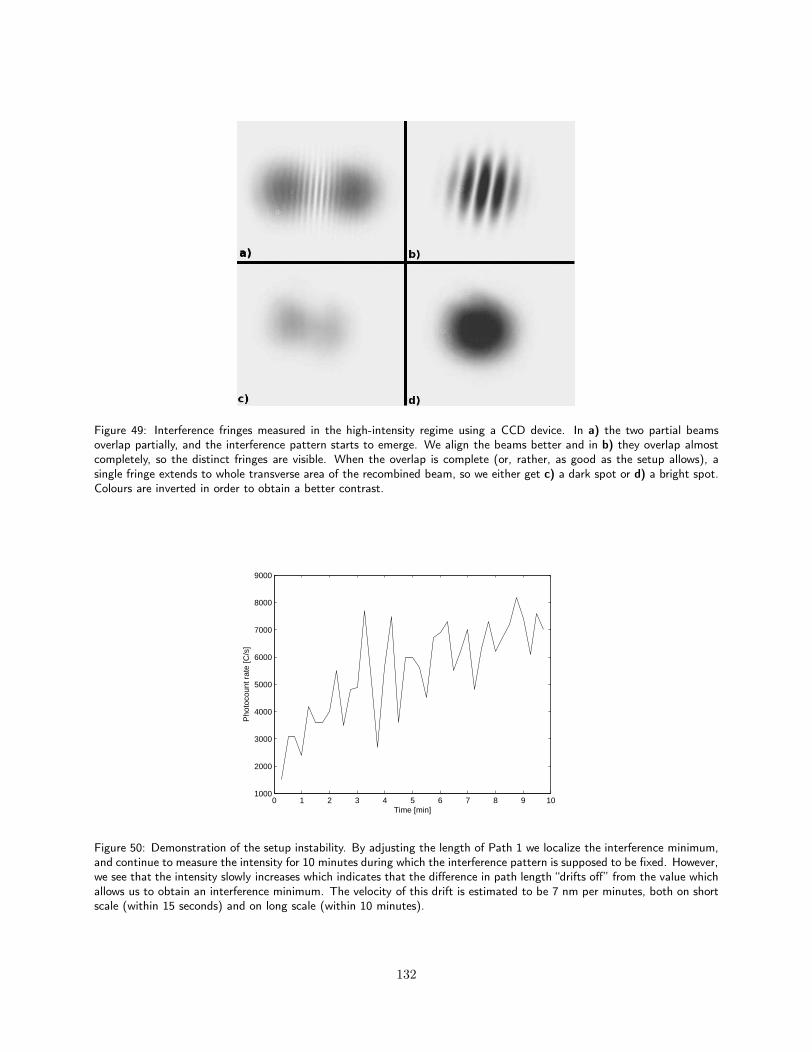
Figure 49: Interference fringes measured in the high-intensity regime using a CCD device. In a) the two partial beamsoverlap partially, and the interference pattern starts to emerge. We align the beams better and in b) they overlap almostcompletely, so the distinct fringes are visible. When the overlap is complete (or, rather, as good as the setup allows), asingle fringe extends to whole transverse area of the recombined beam, so we either get c) a dark spot or d) a bright spot.Colours are inverted in order to obtain a better contrast.

0 1 2 3 4 5 6 7 8 9 101000

2000

3000

4000

5000

6000

7000

8000

9000

Time [min]

Pho

toco

unt r

ate

[C/s

]

Figure 50: Demonstration of the setup instability. By adjusting the length of Path 1 we localize the interference minimum,and continue to measure the intensity for 10 minutes during which the interference pattern is supposed to be fixed. However,we see that the intensity slowly increases which indicates that the difference in path length “drifts off” from the value whichallows us to obtain an interference minimum. The velocity of this drift is estimated to be 7 nm per minutes, both on shortscale (within 15 seconds) and on long scale (within 10 minutes).

132

−500 −400 −300 −200 −100 0 100 200 300 4000

0.5

1

1.5

2

2.5

3x 10

4

Relative path length difference [nm]

Pho

toco

unts

[C/s

]

theorymeasurements

Figure 51: The intensity curve obtained in the Mach-Zender interferometry experiment. The variation of the intensity(or the photocount rate) reflects the presence of an interference pattern there minima and maxima are moving across thedetector aperture when we vary the difference in path lengths of the two partial beams. Note that the path length difference∆d is relative, i.e. we give it relatively to the value where there occurs an intensity minimum. ∆d is varied by regulatingvoltage V of the piezoelectric element which controls the position of one of the mirrors. We assume that the relationbetween V and ∆d is linear, and that after we have increased V in order to “move” from one intensity maximum to thenext one, then ∆d has changed with one wavelength, or 633 nm. We observe that the agreement between the theory andthe experimental results is very good, and the rather large uncertainties are due to short averaging of every measurement.

The uncertainties (i.e. the standard deviations) are rather large, but this is due to the setup instability and

the aforementioned necessity of short averaging (only 10 single photocount measurements54 for a given value

of ∆d). The visibility V of the interference pattern is, according to the standard formula:

V ≡ Imax − Imin

Imax + Imin

= 95.3% ± 5.9%,

where Imax(Imin) is the maximal (minimal) observed intensity. The value of V is high, although the large

uncertainty is again due to the short averaging of single measurements.

7.2.4 Conclusion

The emergence of the interference pattern must be considered in the context of the very low intensity

regime that the experiment has been performed in. We have seen above that the intensity of the original beam

corresponds, in the corpuscular model, to ca. 300.000 photons per second. Given their necessary Poissonian

distribution (see simulations in Ch. 7.1) the mean distance between two consecutive photons in the beam

is 1 km. This distance is almost three orders of magnitude larger than the dimension of the interferometer

(ca. 2.5 m). Thus we naturally expect that at almost any given time there is only one photon present in

the apparatus, and the wave aspect of the radiation – which causes the interference phenomenon – has to be

associated with single photons.

54A single photocount measurement extends over a time window of 1 µs, but in practice each measurement takes 1.5 s due tothe necessity of data processing.

133

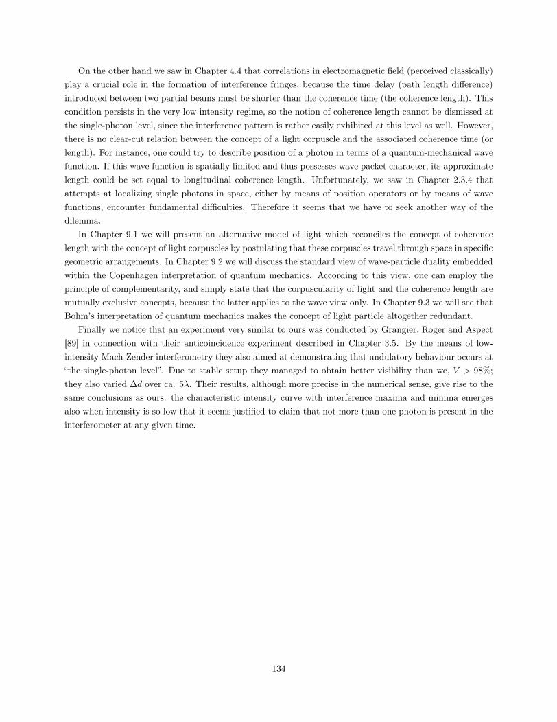
On the other hand we saw in Chapter 4.4 that correlations in electromagnetic field (perceived classically)

play a crucial role in the formation of interference fringes, because the time delay (path length difference)

introduced between two partial beams must be shorter than the coherence time (the coherence length). This

condition persists in the very low intensity regime, so the notion of coherence length cannot be dismissed at

the single-photon level, since the interference pattern is rather easily exhibited at this level as well. However,

there is no clear-cut relation between the concept of a light corpuscle and the associated coherence time (or

length). For instance, one could try to describe position of a photon in terms of a quantum-mechanical wave

function. If this wave function is spatially limited and thus possesses wave packet character, its approximate

length could be set equal to longitudinal coherence length. Unfortunately, we saw in Chapter 2.3.4 that

attempts at localizing single photons in space, either by means of position operators or by means of wave

functions, encounter fundamental difficulties. Therefore it seems that we have to seek another way of the

dilemma.

In Chapter 9.1 we will present an alternative model of light which reconciles the concept of coherence

length with the concept of light corpuscles by postulating that these corpuscles travel through space in specific

geometric arrangements. In Chapter 9.2 we will discuss the standard view of wave-particle duality embedded

within the Copenhagen interpretation of quantum mechanics. According to this view, one can employ the

principle of complementarity, and simply state that the corpuscularity of light and the coherence length are

mutually exclusive concepts, because the latter applies to the wave view only. In Chapter 9.3 we will see that

Bohm’s interpretation of quantum mechanics makes the concept of light particle altogether redundant.

Finally we notice that an experiment very similar to ours was conducted by Grangier, Roger and Aspect

[89] in connection with their anticoincidence experiment described in Chapter 3.5. By the means of low-

intensity Mach-Zender interferometry they also aimed at demonstrating that undulatory behaviour occurs at

“the single-photon level”. Due to stable setup they managed to obtain better visibility than we, V > 98%;

they also varied ∆d over ca. 5λ. Their results, although more precise in the numerical sense, give rise to the

same conclusions as ours: the characteristic intensity curve with interference maxima and minima emerges

also when intensity is so low that it seems justified to claim that not more than one photon is present in the

interferometer at any given time.

134

8 The Afshar experiment

The Afshar experiment which has recently revived the discussion surrounding the wave-particle duality has

not been considered in Chapter 3. Due to its recent character and controversial nature we have chosen to

postpone the presentation of the experiment to the present chapter. It will serve us to illustrate the duality

problem from a general point of view, and motivate our examination of alternative physical models of light

and alternative interpretations of quantum mechanics in Chapter 9.

We begin the following chapter by describing the setup and the results of the experiment (Ch. 8.1). Then

we discuss Afshar’s analysis in the light of the criticism that has been raised against it, and the response of

Afshar and his collaborators (Ch. 8.2). Concluding remarks are given (Ch. 8.3).

8.1 Description and results

The Afshar experiment was conceived in order to challenge the notion55 that the wave- and particle-aspect

of radiation are mutually incompatible, i.e. that it is impossible to simultaneously obtain in any single

interferometry experiment a fully visible interference pattern (corresponding to the wavelike property) and

a complete which-way (“welcher-Weg”) information (correspoding to the particlelike property). Thus, if we

conduct a double-slit experiment with light it is possible to obtain a fully visible (in the sense of Eq. (171)

below) interference pattern suggesting that the single photons have wave nature. However, if one chooses

to place a detector behind one of the slits in order to obtain the information about which slit the photon

“actually” went through, then the interference pattern will no longer be present. In some setups there is a

possibility for obtaining a partial (i.e. not fully visible) interference pattern and partial (i.e. not completely

certain) which-way information. In such situations it has been shown that the following inequality, called the

Greenberger-Yasin inequality, must hold [124]:

V 2 +K2 ≤ 1, (170)

55This notion, firmly rooted in the standard interpretation of quantum mechanics, is due to Bohr and we will explore it indepth in Chapter 9.2. Another interpretation and its possible meaning for the duality problem will also be considered in thatchapter.

135

where V ∈ [0, 1] is the visibility of the interference pattern defined as:

V ≡ Imax − Imin

Imax + Imin

, (171)

with Imax(Imin) being the maximal (minimal) observed intensity in the interference fringes. On the other

hand, K ∈ [0, 1] quantifies the which-way information; K = 1 corresponds to full knowledge about which

way the corpuscle went through, and K = 0 corresponds to no such knowledge at all. K is defined as:

K ≡ 2P − 1

where P is the probability that the light corpuscle went through a particular slit.

Although Eq. (170) was rigourously demonstrated in several ways (besides Greenberger and Yasin [124],

see Jaeger, Shimony and Vaidman [125] and Englert [126]), its practical validity may be questioned, and

we will come back to this issue in Chapter 8.3. For now we describe the Afshar experiment and explain its

relation to Eq. (170).

The Afshar experiment has been described for the first time in 2005 [45], but in the following we will refer

to the paper published in 2007 [46] in collaboration with Flores, McDonald and Knoesel where an improved

version was presented. The experimental setup is shown in Fig. 52. Quasi-monochromatic diode laser light of

wavelength λ = 638 nm from a diode laser with low photon flux passed through an aperture and was incident

onto a pair of pinholes. Their diameters were 40 µm each, and their center-to-center separation was 250

µm. The two beams emerging from the pinholes overlapped in the far-field behind the pinhole screen, and

produced an interference pattern consisting of light and dark fringes. At a distance 0.55 m behind the pinholes

there were placed six thin wires of 127 µm diameter. The separation between two wires was approximately

1.3 mm. The locations of the wires corresponded to the locations of the minima of the interference pattern

(with an accuracy of ±10µm).

The dual pinhole system was imaged by a lens system (placed behind the wires) onto two single-photon

counting modules in such a way that pinhole A was imaged on detector 1, and pinhole B on detector 2. When

the two pinholes were opened and the wire grid was removed, the peak photocount rate registered by each

detector was approximately 104 C/s (see Fig. 52a). When the wire grid was inserted, the photocount rates

were reduced only slightly: by 0.31% for detector 1 and by 1.13% by detector 2 (see Fig. 52b). It suggested

the presence of a destructive interference pattern at the position of the wires, because otherwise (i.e. if no

interference pattern were present) a larger fraction56 of the incoming light should be scattered by the wires.

This was demonstrated by blocking pinhole A or B, while the wire grid remained in place. When only one

of the pinholes was opened, the peak photocount rate of the corresponding detector dropped to ca. 85% of

the original value (i.e. the one from Fig. 52a), and the peak photocount rate of the second detector dropped

to only 0.46% of the original value (see Fig. 52cd).

The authors concluded that in the case with both pinholes opened and the wire grid inserted, a destructive

interference pattern was fully developed at the position of the wires, and at the same time one obtained a full

which-way information about photons passing through apparatus. Besides, these photons had to be single,

since with the low flux the average distance between succesive photons (ca. 10 km) was much larger than

both the dimension of the apparatus and than the coherence length of the laser light used (0.4 m).

In order to demonstrate a violation of the Greenberger-Yasin inequality (Eq. (170)) Afshar et al. estimated

56The losses that were present were due to the finite thicknesses of the wires and imperfect alignment.

136

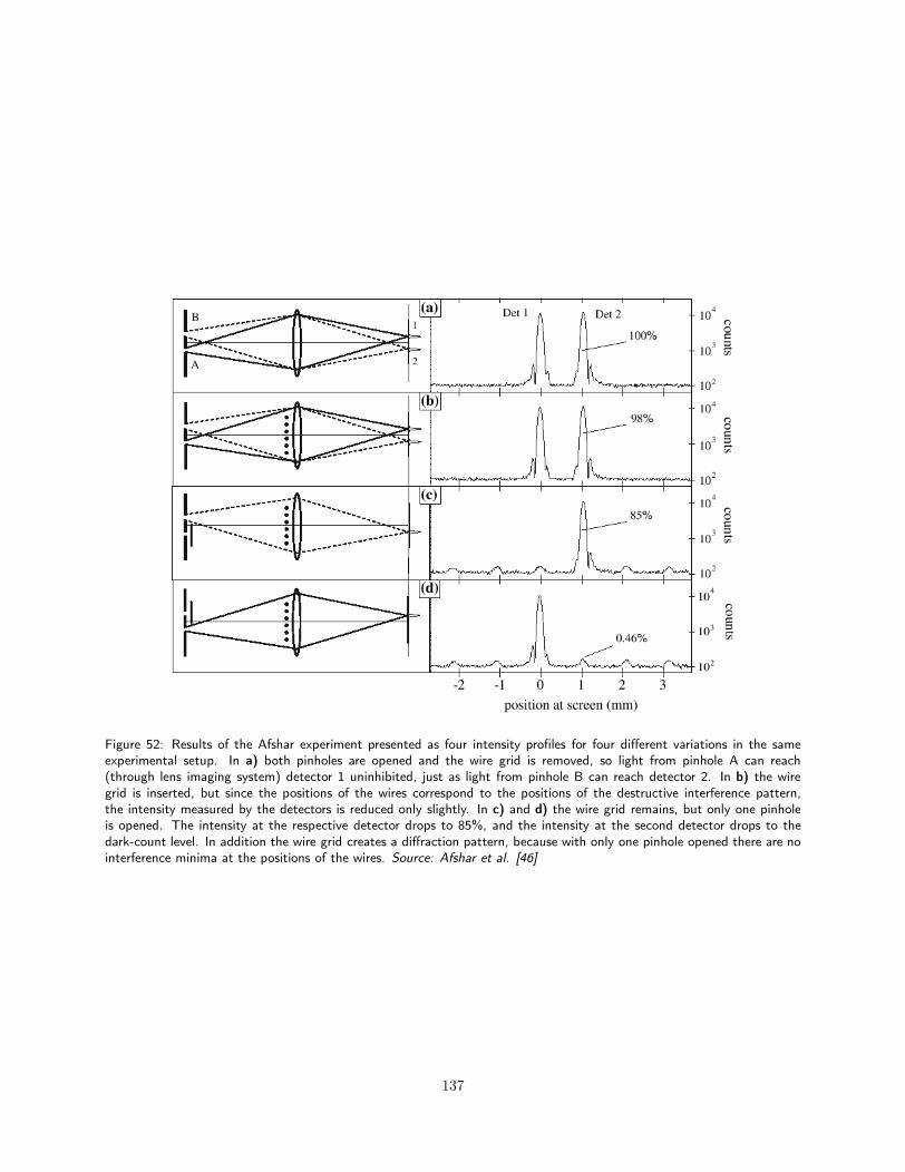
Figure 52: Results of the Afshar experiment presented as four intensity profiles for four different variations in the sameexperimental setup. In a) both pinholes are opened and the wire grid is removed, so light from pinhole A can reach(through lens imaging system) detector 1 uninhibited, just as light from pinhole B can reach detector 2. In b) the wiregrid is inserted, but since the positions of the wires correspond to the positions of the destructive interference pattern,the intensity measured by the detectors is reduced only slightly. In c) and d) the wire grid remains, but only one pinholeis opened. The intensity at the respective detector drops to 85%, and the intensity at the second detector drops to thedark-count level. In addition the wire grid creates a diffraction pattern, because with only one pinhole opened there are nointerference minima at the positions of the wires. Source: Afshar et al. [46]

137

the which-way information K directly and inferred the value of V by assuming a presence of an interference

pattern with worst possible visibility, but compatible with their data. In their calculations K ≥ 0.97 and

V ≥ 0.64, so K2 +V 2 ≥ 1.35 and the inequality was clearly violated. According to the authors, the outcome

of the Afshar experiment indicates that the particlelike and the wavelike aspect of radiation may be present

simultaneously in a single experimental setup, where the notion of simultanity has been used in the sense

given by the inequality. Taken the results to be correct, we will examine the implications of this simultanity

claim in Chapter 8.3. First, however, we review a critical response to the Afshar experiment which casts in

doubt the validity of the results.

8.2 Criticism of the experiment

We stress that the results of the Afshar experiment did not offer (and did not aim at offering) any natural

explanation to the wave-particle duality problem, but rather challenged the principle of complementarity

associated with the duality. The principle of complementarity, due to Niels Bohr [127], represents the central

feature of the standard (Copenhagen) interpretation of quantum mechanics. Both complementarity and the

standard interpretation will be examined in detail in Ch. 9.2. For now, suffice it to say that complementarity

implies the mutual exclusiveness of the corpuscular and the undulatory aspect of the nature of radiation

in the double-slit (or double-pinhole) experiment. This exclusiveness is quantified by Eq. (170). Thus, by

demonstrating the invalidity of Eq. (170) in their particular setup, Afshar et al. seemed to undermine the

principle of complementarity itself.

Not surprisingly, the authors’ analysis and interpretation of the experimental results were met with

considerable amount of criticism. Kastner [128] pointed out that Afshar et al. had confused which-way

information with which-slit information. This claim was later rebutted by Flores and Knoesel [129] who

presented a modified, but equivalent version of the Afshar experiment, so the remarks of Kastner no longer

applied. In another critical paper Drezet [130] concluded however that Afshar et al. had misused Eq. (52) by

using one ensemble of photons for calculating V , and another ensemble for calculating K; qualitatively such

a conclusion condenses to the demand that the interference pattern cannot be simply inferred, but must be

actually measured. According to Qureshi [131], however, the existence of interference pattern in the Afshar

experiment is genuine and it can be inferred, but its presence destroys the which-way information, because

measuring a photon by, say, detector 1 (see Fig. 52) does not longer guarantee that the photon originally

emerged from pinhole A.

Qureshi’s point has been pursued by Steuernagel [132] who presented a rather detailed quantitative

analysis of the Afshar experiment in the framework of wave optics. On the basis of his calculations he could

conclude that when the wire grid is inserted, the path detection becomes in fact less reliable. When the wires

are positioned in the minima of the interference pattern, the direction of the first diffraction order for photons

emerging from pinhole A (B) points towards the “wrong” detector, i.e. detector 2 (1). In fact the intensity

profiles from Fig. 52, if properly interpreted, demonstrate this phenomenon. As we have alread seen, when

the wire grid is inserted and one of the pinholes, say pinhole A, is closed (Fig. 52c), the photocount rate

of detector 2 is reduced to 85% of the original value, and the photocount rate of detector 1 is reduced to

dark-count level. If we now open the pinhole A, it seems that the original (i.e. the one from Fig. 52a)

intensity profile has been recovered, but the similarity of profiles from Fig. 52a and Fig. 52b is misleading.

138

As Steuernagel points out: “The increase of the count rates (...) is due to a partial compensation of the

effects of the grid, but not their complete circumvention. This partial compensation arises at the expense

of redirecting light to the “wrong” detector” (Steuernagel [132], p. 1378). So the fact that in Fig. 52b we

again observe two distinct peaks with approximately the same height as in Fig. 52a does not mean that all

photocounts of detector 1 (2) are caused by photons emerging from pinhole A (B), because now the wire grid

causes diffraction and (partial) “mixing” of the path from pinhole 1 to detector A with the path from pinhole

2 to detector B.

Steuernagel proceeded to show that when this diffraction effect is taken into account, the which-way

information K is accordingly reduced. The LHS of Eq. (170) becomes a function of wire thickness, but never

exceeds one. In fact, the optimal situation with V 2 +K2 = 1 is achieved only when the grid is completely

absent, or when the wires are so thick that only very small slits remain open between them, and effectively

instead of a wire grid we have a screen onto which the interference pattern is imaged. Steuernagel estimated

that the correct value for the sum V 2 +K2 in Afshar’s experiment is 0.813 at best. According to him, the

error in the calculations of Afshar et. al was due to the fact that they determined V by considering the

photons reflected by the wire grid, while K was determined by considering the photons transmitted to the

detectors. This is emphatically not allowed, because these two photon ensembles are mutually exclusive, and

the complementarity principle embodied in the Greenberger-Yasin inequality (Eq. (170)) must be applied to

them separately.

Steuernagel’s comments were answered by Flores [133], one of the original authors, who highlighted an

important feature of Afshar’s experiment. This feature had been apparently underestimated by Steuernagel

and other critics. Flores recalled that the photon rate used in the experiment had been so low that the aver-

age separation between succesive photons exceeded the size of the experimental apparatus by four orders of

magnitude. Therefore it was reasonable to claim that at any given time there was only a single light particle

(in the corpuscular model) present in the apparatus. Flores reasoned that in such circumstances separating

these single photons into two mutually exclusive ensembles constituted an arbitrary division, because in the

same spirit one could introduce an infinite number of mutually exclusive ensembles, one for each point of

space where a photon could possibly be absorbed, thus rendering any analysis of visibility and which-way

information impossible. What was of importance, according to Flores, was that each single photon entering

the setup was subjected to the same experimental conditions. Flores argued further that Steuernagel in his

quantitative analysis had used two different ensembles of photons when calculating the visibility, so that his

criticism actually applied to his own approach. Flores, however, did not address explicitly the other problem

pointed out by Steuernagel, i.e. the fact that the presence of the wire grid redirected light to the “wrong”

detector.

8.3 Concluding remarks

Afshar’s experiment and the surrounding discussion motivates us in reassessing the wave-particle duality from

a more general point of view. In the Introduction we have defined the wave-particle duality as the phenomenon

where electromagnetic radiation and particles can exhibit either wavelike or particlelike behaviour, but not

both. In the thesis the emphasis has been put on the problem of reconciliating these two models and

presenting the difficulties they both exhibit in theoretical frameworks and experimental setups. Afshar et al.

139

do not set out to propose and verify any alternative model of light; their goal is to examine the postulate that

radiation cannot behave as waves and as particles simultaneously, and to eventually show that the inequality

embodying this postulate, Eq. (170), is invalid, at least in the case of some non-perturbative measurement

processes.

Such refutation (if unambigouous) would of course revolutionize quantum mechanics, because it would

empirically rebut the principle of complementarity on which the standard interpretation of the theory rests

(see Ch. 9.2). The rebutal would then stimulate the interest in searching alternative models of matter and

radiation. On the other hand it is rather striking that most of the parts involved in the analysis of Afshar’s

experiment (i.e. Afshar et al. themselves, Steuernagel etc.) implicitly employ the customary approach to

the nature of light: They switch arbitrarily between the undulatory and the corpuscular model, depending

on which one is most suitable at any given moment in their treatments. For instance, Afshar et al. in

their paper [46] resort exclusively to the corpuscular model and do not assign to the photons any wavelike

properties. The question of how the single photons passing the apparatus actually interfered destructively

with themselves at the wire grid, so they could proceed uninhibited to the respective detectors, was left out

altogether. Steuernagel [132], however, makes heavily quantitative use of the wave model. Therefore Flores

[133] is able to oppose his criticism by the simple remark about photons being present in the apparatus one

at a time, but then again he subdues the undulatory aspect of the phenomena involved.

Of course, as long as the analysis of Eq. (170) proceeds in the usual framework of the wave-particle

duality (where one sometimes employs the corpuscular view, and sometimes the undulatory view, depending

on circumstances), such an inconsistent approach is per assumption allowed. However, one has to keep in

mind that the equation has been derived for a very specific experimental situation, i.e. that of a double-slit

(or double-pinhole) experiment without any wire grids or additional elements present in the setup, so the

class of experiments that Eq. (170) applies to is rather narrow. Furthermore, it is not clear whether we

are allowed to infer (or partially infer) visibility and / or which-way information as Afshar et. al did, and

how “inference” and “actual measurement” should be defined57. Preconceived judgments play some role in

experiments of any kind (and in analysis of their results), so in the case of the wave-particle duality one

should a priori and explicitly declare to which degree one will allow himself to be steered by them. Such a

declaration is missing from both the paper of Afshar et al. [46] and from Steuernagel’s criticism [132].

Another crucial point, which has apparently been missed by most participants of the discussion, is that

Afshar’s experiment could be explained in its entirety using only the undulatory model. Closer inspection

shows that explicit introduction of corpuscle-like behaviour into the analysis is redundant, because, as we

have seen in Section 5.1.2, the discreteness of the photodetection process can be easily accommotated by the

semiclassical model. In such a situation the concept of which-way information becomes meaningless, and

the parameter K from Eq. (170) disappears (or it could be reinterpreted as some kind of ratio between the

intensity fluxes reaching the detectors, but in this version its significance is dubious). Steurnagel’s analysis

lies rather close to the fully undulatory approach, but the concept of photon is nonetheless employed in

connection with the detection process.

Thus it might be said that the conflict between the undulatory and the corpuscular view of light is not

really present in Afshar’s experiment as it stands. It would be, however, interesting to consider for instance

a combination of Afshar’s experiment and Grangier-Roger-Aspect experiment (see Ch. 3.5), because as we

have noted before, it is the anticoincidence that serves to exhibit corpuscular properties more clearly. On its

57We notice that any measurement is in fact an inference, because we use the experimentally obtained data to ascribe numericalvalues to physical quantities under examination.

140

own, Afshar’s experiment embodies first and foremost a clever non-perturbative measurement scheme with

possibly interesting further extensions, but is link to the essence of the wave-particle duality is not as direct

as one could believe.

Even if we would manage to unambigously demonstrate that Eq. (170) applies to the setup of Afshar’s

experiments, and even if we would agree on the fact that the data obtained breaks the inequality, the undu-

latory and corpuscular aspects of radiation would still remain complementary (in the usual, not Bohresque,

sense of the word), because the experiment does not try to reduce them to any underlying physical theory58.

In order to reconcile the two models, one has to take a step back and either propose a priori an alternative

physical model of light, or even try to explain the duality in the framework of an alternative interpretation

of quantum mechanics. This will be done in the next chapter.

58This is not an accusation – because Afshar et al. did not aim for such reduction – but only an observation regarding themeaning of the experiment.

141

142

9 Explaining the wave-particle duality

In the following chapter we will discuss how the wave-particle duality of light could be possibly expounded

and its higly problematic nature elucidated. The word “expounding” is used here in the sense of giving such

a picture of the physical world where both the corpuscular and the undulatory properties emerge from some

underlying principle. This can be achieved in two distinct ways. Firstly, we could try to give an alternative

model for the structure of light. In the long run such a model must be of course consistently incorporated into

the more general framework of quantum mechanics, but to begin with it would be instructive to consider the

model “on its own” and discuss its inherent assets, weaknesses and possible new predictions. Secondly, one

could try to explain the wave-particle duality by modifying, or even replacing, the standard interpretation of

quantum mechanics with which the duality is intimately connected.

The first approach will be presented in Chapter 9.1 where we examine the so-called “photon clump” model

that aims at a direct elimination of the duality paradox of light. The role that the wave-particle duality plays

in the standard interpretation of quantum mechanics is given in Chapter 9.2 which precedes examination of the

radically different Bohmian interpretation in Chapter 9.3. We will see that while the standard interpretation

deems questions about the wave-particle duality meaningless, the Bohmian interpretation manages to answer

them directly.

We must, however, stress two things. First and foremost, the following chapter is much more speculative

than the rest of the thesis. The author does not assume that the proposed explanations are correct; he simply

intends to show how the wave-particle duality problem could be solved according to models and interpreta-

tions worked out by other physicists. Secondly, up until now the thesis has been concerned with the duality

of light, but when examining different interpretations of quantum mechanics we will be forced to expand our

perspective and include the duality of matter into the discussion (see Appendix C for general discussion of

matter waves).

9.1 The “photon clump” model

9.1.1 Basic assumptions

In order to reconcile the undulatory and the corpuscular models of light, one could postulate that the

pointlike particles of light – photons – travel through space in specific geometric arrangements which reflect

their wavelike properties. We will in the following review the “photon clump” model proposed by Panarella

[71] which rests on that notion and incorporates additional assumptions about the behaviour of such “photon

143

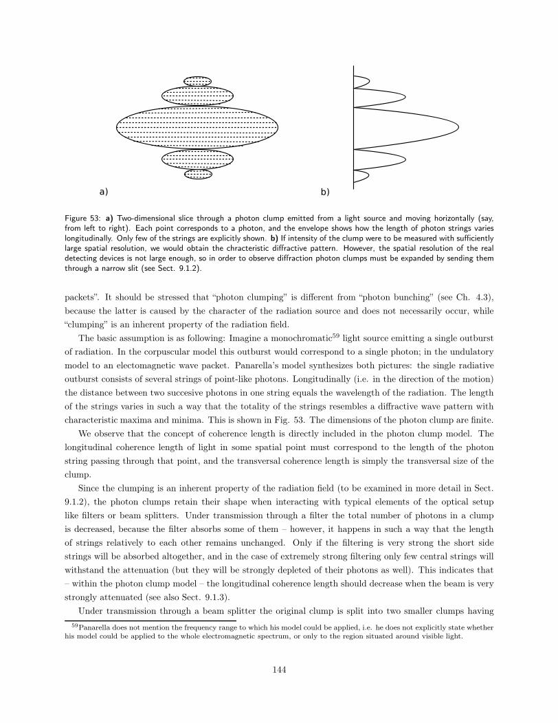
Figure 53: a) Two-dimensional slice through a photon clump emitted from a light source and moving horizontally (say,from left to right). Each point corresponds to a photon, and the envelope shows how the length of photon strings varieslongitudinally. Only few of the strings are explicitly shown. b) If intensity of the clump were to be measured with sufficientlylarge spatial resolution, we would obtain the chracteristic diffractive pattern. However, the spatial resolution of the realdetecting devices is not large enough, so in order to observe diffraction photon clumps must be expanded by sending themthrough a narrow slit (see Sect. 9.1.2).

packets”. It should be stressed that “photon clumping” is different from “photon bunching” (see Ch. 4.3),

because the latter is caused by the character of the radiation source and does not necessarily occur, while

“clumping” is an inherent property of the radiation field.

The basic assumption is as following: Imagine a monochromatic59 light source emitting a single outburst

of radiation. In the corpuscular model this outburst would correspond to a single photon; in the undulatory

model to an electomagnetic wave packet. Panarella’s model synthesizes both pictures: the single radiative

outburst consists of several strings of point-like photons. Longitudinally (i.e. in the direction of the motion)

the distance between two succesive photons in one string equals the wavelength of the radiation. The length

of the strings varies in such a way that the totality of the strings resembles a diffractive wave pattern with

characteristic maxima and minima. This is shown in Fig. 53. The dimensions of the photon clump are finite.

We observe that the concept of coherence length is directly included in the photon clump model. The

longitudinal coherence length of light in some spatial point must correspond to the length of the photon

string passing through that point, and the transversal coherence length is simply the transversal size of the

clump.

Since the clumping is an inherent property of the radiation field (to be examined in more detail in Sect.

9.1.2), the photon clumps retain their shape when interacting with typical elements of the optical setup

like filters or beam splitters. Under transmission through a filter the total number of photons in a clump

is decreased, because the filter absorbs some of them – however, it happens in such a way that the length

of strings relatively to each other remains unchanged. Only if the filtering is very strong the short side

strings will be absorbed altogether, and in the case of extremely strong filtering only few central strings will

withstand the attenuation (but they will be strongly depleted of their photons as well). This indicates that

– within the photon clump model – the longitudinal coherence length should decrease when the beam is very

strongly attenuated (see also Sect. 9.1.3).

Under transmission through a beam splitter the original clump is split into two smaller clumps having

59Panarella does not mention the frequency range to which his model could be applied, i.e. he does not explicitly state whetherhis model could be applied to the whole electromagnetic spectrum, or only to the region situated around visible light.

144

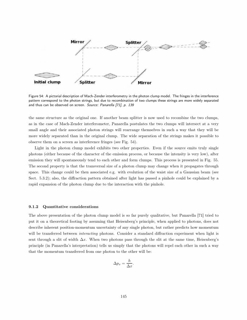
Figure 54: A pictorial description of Mach-Zender interferometry in the photon clump model. The fringes in the interferencepattern correspond to the photon strings, but due to recombination of two clumps these strings are more widely separatedand thus can be observed on screen. Source: Panarella [71], p. 139

the same structure as the original one. If another beam splitter is now used to recombine the two clumps,

as in the case of Mach-Zender interferometer, Panarella postulates the two clumps will intersect at a very

small angle and their associated photon strings will rearrange themselves in such a way that they will be

more widely separated than in the original clump. The wide separation of the strings makes it possible to

observe them on a screen as interference fringes (see Fig. 54).

Light in the photon clump model exhibits two other properties. Even if the source emits truly single

photons (either because of the character of the emission process, or because the intensity is very low), after

emission they will spontaneously tend to each other and form clumps. This process is presented in Fig. 55.

The second property is that the transversal size of a photon clump may change when it propagates through

space. This change could be then associated e.g. with evolution of the waist size of a Gaussian beam (see

Sect. 5.3.2); also, the diffraction pattern obtained after light has passed a pinhole could be explained by a

rapid expansion of the photon clump due to the interaction with the pinhole.

9.1.2 Quantitative considerations

The above presentation of the photon clump model is so far purely qualitative, but Panarella [71] tried to

put it on a theoretical footing by assuming that Heisenberg’s principle, when applied to photons, does not

describe inherent position-momentum uncertainty of any single photon, but rather predicts how momentum

will be transferred between interacting photons. Consider a standard diffraction experiment when light is

sent through a slit of width ∆x. When two photons pass through the slit at the same time, Heisenberg’s

principle (in Panarella’s interpretation) tells us simply that the photons will repel each other in such a way

that the momentum transferred from one photon to the other will be:

∆px =h

∆x.

145

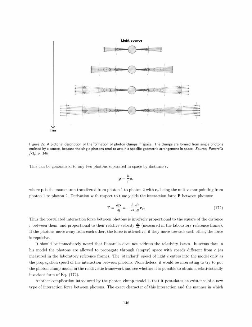
Figure 55: A pictorial description of the formation of photon clumps in space. The clumps are formed from single photonsemitted by a source, because the single photons tend to attain a specific geometric arrangement in space. Source: Panarella[71], p. 140

This can be generalized to any two photons separated in space by distance r:

p =h

rer

where p is the momentum transferred from photon 1 to photon 2 with er being the unit vector pointing from

photon 1 to photon 2. Derivation with respect to time yields the interaction force F between photons:

F =dp

dt= − h

r2dr

dter. (172)

Thus the postulated interaction force between photons is inversely proportional to the square of the distance

r between them, and proportional to their relative velocity drdt (measured in the laboratory reference frame).

If the photons move away from each other, the force is attractive; if they move towards each other, the force

is repulsive.

It should be immediately noted that Panarella does not address the relativity issues. It seems that in

his model the photons are allowed to propagate through (empty) space with speeds different from c (as

measured in the laboratory reference frame). The “standard” speed of light c enters into the model only as

the propagation speed of the interaction between photons. Nonetheless, it would be interesting to try to put

the photon clump model in the relativistic framework and see whether it is possible to obtain a relativistically

invariant form of Eq. (172).

Another complication introduced by the photon clump model is that it postulates an existence of a new

type of interaction force between photons. The exact character of this interaction and the manner in which

146

it should be mediated is completely unknown, and it seems that there is no experimental evidence indicating

that such an interaction exists60. The ratios between the postulated interaction force FI and the electrostatic

and gravitational forces, respectively denoted by FE and FG, are:

FI

FE≈ 10−6 ×

(

dr

dt

)

FI

FG≈ 1037 ×

(

dr

dt

)

.

Despite the difficulties mentioned in the two previous paragraphs, Panarella continued his analysis by

deriving Kirchhoff’s theorem using the concept of interacting photons. Kirchhoff’s theorem (see Born and

Wolf [134], p. 378) may be taken as the starting point for classical diffraction theory, so other results as-

sociated with diffraction phenomena will follow from it. In Panarella’s approach, however, the theorem no

longer applies to the amplitudes of the electromagnetic waves, but to a type of optical disturbance which is

related to the total momentum transfer between photons. By deriving Kirchhoff’s theorem Panarella claimed

that Eq. (172) is able to quantitatively explain the diffraction phenomena. Furthermore he showed than

when a collection of propagating photons enters equilibrium, the distance between successive photons equals

wavelength of the (monochromatic) radiation involved. Here, however, he had to refer to de Broglie’s relation

λ = hp (see Appendix C).

9.1.3 Concluding remarks

The photon clump model represents a possibility of reconciling the wave and the corpuscular models of

radiation. Even if the model were to be refuted by empirical observations, it illustrates nonetheless how an

alternative model of light, aiming at explaining the wave-particle duality and building on a rather simple

idea, necessitates rather bold claims about the physical reality. On one hand, the basic assumption of the

photon clump model is hardly innovative: it simply states that the collective behaviour of light corpuscles

gives rise to undulatory behaviour of these. On the other hand, we see that the model, taken only a few steps

further, exhibits a strongly speculative character, since it postulates existence of a new interaction force.

But as the history of physics has taught us, speculations are always necessary in order to resolve problems

concerning the nature of reality.

It seems that the idea that the collective behaviour of light corpuscles is responsible for the observed

undulatory effects was already refuted by interference and coincidence experiments performed at intensities

so low that the claim of one photon being present in the apparatus at any given time was fully justified.

However, Panarella argues that the outcomes of such experiments (as the Jánossy experiment, see Ch. 3.2,

or the Grangier-Roger-Aspect experiment, see Ch. 3.5) are not unambiguous: In the case of the Jánossy

experiment, the one-photon-at-any-time claim was presented a priori and not verified in any way, and in

the case of the Grangier-Roger-Aspect experiment, the limited quantum efficiency of the detectors made the

authors unable to recognize photon clumps if they indeed had been present. These reservations were already

mentioned when discussing the two experiments.

Panarella’s theory, as any new physical model, should be judged by accordance of its predictions with the

60Unless, of course, we take the problematic wave-particle duality phenomena to be the required indication.

147

empirical results. The photon clump model gives several predictions. First, in order to obtain with certainty

single photons from a clump, one should break it up both transversally (e.g. using a very small pinhole) and

longitudinally (e.g. using some kind of chopper). The single photons should then be devoid of any wavelike

properties. If one employs very strong filtering instead, it is possible that some clumps after transmission

will partially retain their original structures, and so they will still exhibit undulatory behaviour.

Secondly, we have already commented that the concept of photon clumps may be made consistent with

the notion of coherence, and that the length of photon strings in a clump may be related to the longitudinal

coherence length of light. Since filtering (at least when its very strong) reduces the string length considerably,

it should also directly influence coherence properties of light. This prediction is not to be found in the classical

theory of coherence (see Ch. 4) according to which the coherence length is not intensity-dependent. On the

other hand, although it seems that this prediction has never been checked explicitly in the laboratory61, there

are no empirical indications that it could be correct.

Finally, the quantitative part of the photon clump model predicts that the equilibrium separation between

neighbouring photons in a clump equals the wavelength λ of the radiation field. When photon number density

(i.e. intensity) of a laser beam is so high that each photon must occupy volume smaller than λ3, the theory

implies that the radiation frequency increases in order to accommodate the “cramping” of the photons.

Panarella gives a numerical example: for a 500 nm laser beam the threshold photon number density allowed

by the photon clump model is 1.52×1013 photons per cm3 which corresponds to intensity of 1.81×105 W/cm2.

If the intensity is increased further, an increase of frequency should result. Such an increase of frequency

could be used in order to explain anomalous photo-ionization of gases and anomalous photoelectric effects

that were observed before (see Panarella [71], p. 165). The anomalous character of these effects consists

of the fact that photo-ionization or photoelectrons are observed, even though the single photon energy is

lower than, respectively, the ionization potential or the work function. However, there exist another, better

developed explanation of these phenomena involving multi-photon scattering (see Girardeau-Montaut and

Girardeau-Montaut [135]).

It remains to be seen whether the photon clump model will be developed further and whether experimen-

talists will be able to substantiate or refute it. Even if Panarella’s model will be dismissed, it will serve to

show why it is very difficult (or impossible) to explain the wave-particle duality by assuming that corpuscular

photons move through space in geometrical, wavelike patterns.

9.2 Complementarity of the Copenhagen interpretation

The core of every well-developed physical theory is a mathematical apparatus that serves to define and relate

different quantities and notions. However, without a proper interpretation that provides a link between

this apparatus and the physical world, the theory would remain only a purely mathematical and abstract

tool. It is the interpretation that enunciates correspondence between the mathematical framework and the

physical reality. It tells us how the mathematical methods are to be used in order to explain the nature of the

world and in order to predict outcomes of diverse experiments (or, more generally: how to quantify natural

phenomena using the given mathematical machinery).

The interpretations of physical theories have always been an important subject for the philosophy of sci-

61In scientific databases there are in fact no articles referring to Panarella’s paper [71].

148

ence. Up until the first half of the twentieth century the interpretations had been rather straight-forwardly

associated with different branches of physical sciences, as Newtonian mechanics, ray optics or thermodynam-

ics, to name a few examples. Even though these interpretations had played a crucial role in shaping of the

human view of the physical world62, in the long run they never presented grave conceptual problems, because

“common sense” was always able to accommodate them.

The situation changed with the arrival of quantum mechanics and its notorious standard interpretation

(also called Copenhagen interpretation) which was developed mainly by Niels Bohr and Werner Heisenberg63

[137]. The standard interpretation emphasized and cemented very peculiar features of the new theory that

early research had already suggested. What was more important, however, was that the interpretation denied

the quantum mechanical formalism any pictorial role in describing the physical world. Bohr claimed64 that

on the atomic level one should never speak of properties inherently attributed to material objects, but always

consider them in the framework of experimental setup that is used to examine and measure them. In other

words, “reality” should not be considered apart from “experiment” (in the sense of an observation), because it

is the “experiment” that determines the nature of “reality”. The answers given by Nature lack epistemological

value, unless they are appreciated together with the questions that observers have posed.

There are many concepts and ideas that constitute the standard interpretation of quantum mechanics65;

in fact, there is no agreement among contemporary scientists regarding how the standard interpretation

should be precisely defined [140]. It is out of the scope of this chapter to give a detailed discussion about how

the standard interpretation emerged historically, how it relates to philosophical issues or what is its exact

meaning for the quantum-mechanical formalism. Among the different elements of the interpretation we will

focus on only one: The notion of complementarity which Bohr employed to explain the wave-particle duality

problem, and which was built around Heisenberg’s uncertainty principle.

The complementarity principle played a rather fundamental role in Bohr’s reasoning and therefore has

been often identified with the Copenhagen interpretation. Complementarity is generally defined as:

[The natural principle according to which] it is not possible to describe atomic phenomena in as

complete a manner as classical ones, since the pairs of conjugate variable that must be known for

an exact description in the latter case are mutually exclusive in the former. From an experimental

point of view there are therefore mutually exclusive descriptions of an atomic system which are

complementary to each other. [141]

Thus, Bohr’s complementarity states that a physical object, examined on the microscopic or atomic level, may

exhibit two contradictory properties, and these properties in principle cannot be reduced to some underlying

physical model of reality. They should be treated, to use a simple metaphor, as opposite sides of one coin.

It is the experimental setup that decides which property of the object will emerge in practice, in the same

way as turning the coin around decides which side of it we look upon.62One of the earliest modern examples is Newton’s realization that an object moving in some reference frame, not subjected

to any forces, will never stop. This opposed the old Aristotelian view according to which any motion must be sustained, or itwould cease otherwise.

63However, Bohr and Heisenberg never fully agreed how the mathematical formalism should be related to the physical world,and none of them ever used the term “the Copenhagen interpretation”. It was conceived by physicists who were opposing theirview [136].

64At least that was his more mature view, becase Bohr’s opinion on the subject evolved with time. For instance, Bohr opposedthe light-quantum hypothesis longer than most physicists of his time (Murdoch [138], p. 22).

65For the summary of Bohr’s own thoughts, see Bohr [139].

149

The complementarity (pushed to the extreme66) embodies the inherent conflict between two fundamental

physical notions: that of space-time localization and that of causality (see Selleri [137], p. 101). If the causality

is analyzed in terms of the conservation of energy and momentum when these are exchanged between systems,

then measuring causality with infinitely large precision implies that the uncertainty in measured energy E

and momentum p is zero, ∆E = ∆p = 0. But then, according to Heisenbergs’ uncertainty principle (see

Appendix A), the measurement has to disturb the space-time localizations (r, t) of the measured objects, and

the disturbance is maximal in the sense that ∆r = ∆t = ∞. Since, as remarked above, it is the observation

that determines the nature of reality, we see that space and time in the above scheme cease to exist, which

is the price that we have to pay for establishing full causality.

On the other hand, if we try to measure space-time localization of a microscopic object without any

uncertainty, so that ∆r = ∆t = 0, the transfer of energy and momentum between the object and the

measuring apparatus must be characterized by complete uncertainty, whence ∆E = ∆p = ∞. Under such

conditions verification of the energy-momentum conservation laws is obviously impossible, and thus the

notion of causality has to be given up, because we are unable to speak about it in physical terms. We infer

that (infinitely precise) observation of space and time is incompatible with (inifinitely precise) observation of

causality, and thus these two notions mutually exclude each other.

The complementarity principle as applied to space, time and causality may now be translated to the

wave-particle duality problem. If we wish to analyze the interaction of radiation and matter in causal terms,

we have to resort to the corpuscular view, because the conservation of energy and momentum is adequately

expressed using the photonic view of radiation and the particle view of matter. In this scheme, however,

we are unable to pinpoint space-time localizations of the corpuscles involved. If we rather want to do that,

then the undulatory picture of radiation and matter must be employed, becaused squared modula of wave

functions give us probabilistic prediction for finding the physical objects at different points. The fact that

this prediction is essentialy stochastic is of course another basic feature of the quantum theory.

Thus we see that radiation and matter pass through space-time in the form of probabilistic waves, and

to describe this propagation the undulatory picture is appropriate. But in their interaction with another

objects the causal considerations are crucial, and then the corpuscular behaviour is exhibited. The standard

interpretation of quantum mechanics answers the question about the nature of light and matter by claiming

that they are neither particles or waves until some specific experimental setup is employed in order to observe

the system. Then the character of the observation forces the system to behave either in a particlelike or in a

wavelike manner.

Within the framework of the standard interpretation the outcome of the double-slit experiment with single

photons (i.e. conducted in the very low intensity regime) can be now explained. A source emits a very weak

outburst of radiation with freqency f . The energy of the outburst is minimal in the sense that it corresponds

to a single quantum of energy E = hf . The quantum propagates through space as a probabilistic wave which

is diffracted by the double-slit screen. If we now let the radiation impinge on the second screen, and if we

repeat the experiment many times, a corresponding diffraction pattern will eventually emerge. However, if

we place a (perfect) detector closely behind, say, the upper slit, we will effectively ask about the space-time

localization of the radiation before it has reached the second screen. Then we will either find out that the

light quantum passed through the upper slit, interacted with the detector and transferred its momentum and

energy in a corpuscle-like manner; or that it passed through the lower slit and impinged on the second screen

66There are many versions of complementarity and it is somewhat unclear whether Bohr himself was among advocates of thestrongest form of the principle. As noticed in two previous footnotes, his views evolved with time.

150

– but now no diffraction pattern is present, because the probabilistic wave could not be diffracted due to the

detector covering one of the slits.

Such an explanation of the wave-particle duality is in some sense unsatisfactory, because instead of giving

a tangible answer to the question about the “true” nature of light, it simply states that this “true” nature

is dual and depends on our measuring instruments. The wavelike property and the particlelike property are

complementary aspects of reality which cannot, in principle, be reduced to any common denominator.

It is interesting to note that Bohr himself did not necesarily treat particle and wave aspects on completely

equal footing. As far as electromagnetic radiation was concerned, Bohr seemed to believe that the undulatory

properties are in an ontological sense superior to the corpuscular properties [137] [138]. His attitude was most

probably due to macroscopic observations of radiation confirming its classical undulatory descriptions. (But

then it should be parallelled by the fact that in the classical limit matter behaves in a corpuscular fashion

while the wave aspect is only an auxilliary concept.)

The Soviet physicist Vladimir Fock developed further the complementary explanation of duality (see

Selleri [137], pp. 103-107). He stressed the claim that considering complementary properties (in their pure

forms) simultaneously is meaningless, because the nature of reality is relative with respect to the means of

observation. These means must be considered in classical terms, but the quantum-mechanical uncertainty

relations still have to be taken into account. In the double-slit experiment any effort to measure a fully

visible diffraction pattern excludes possiblity of obtaining information about which slit the light quantum

has travelled through. The means of observation are incompatible, and thus the wavelike and the particlelike

properties are (according to Fock) incompatible also.

In Chapter 8, however, we have investigated whether these properties can be observed simultaneously

in the sense of violating the Greenberger-Yasin inequality (Eq. (170) on p. 135), and we have seen that

the results of Afshar experiment are inconclusive. Even if future research establishes with certainty that

the experiment does not violate the equation, and that the equation indeed cannot be violated, it would

still allow us to observe partially visible interference pattern and to obtain partial which-way information

(Wootters and Zurek, [143]). Thus Bohr’s complementarity, strictly speaking, applies only to the pure forms

of the undulatory or corpuscular behaviour. Furthermore, we have to remember that the key point of Bohr’s

reasoning is the assumption that if two properties cannot be observed simultaneously, then they cannot be

both real independently of experiment. But this assumption is philosophical rather than physical which

encourages us to question it and seek other interpretations of quantum mechanics that do manage to reduce

the undulatory and corpuscular properties to a single underlying model. Probably the most important of

these alternative interpretations will be presented in the following section.

9.3 The Bohmian interpretation of quantum mechanics

An alternative interpretation of the quantum-mechanical formalism was proposed in 1952 by David Bohm

[144] [145]. During the second half of the 20th century it has evolved through several stages. The evolution

is reflected in its different names: Originally it was called “an interpretation in terms of ’hidden’ variables”,

but later renamed to “causal interpretation”, and finally to “ontological interpretation”. Sometimes it was

also called de Broglie-Bohm theory in order to emphasize the similarities between Bohm’s and de Broglie’s

approach to quantum mechanics [39]. For simplicity, in the following we will simply call it “the Bohmian

151

interpretation”.

Bohm opposed the Copenhagen interpretation by claiming that quantum mechanics should be ontolog-

ically applied to our understanding of Nature, instead of being merely treated as an epistemological tool.

Thus, the Bohmian interpretation ascribes physical reality to microscopic phenomena in the same manner as

classical physics ascribes reality to macroscopic phenomena. In the framework of the Bohmian interpretation

the formalism of quantum mechanics does not only predict the results of measurements in an algorithmic

manner – the Bohmian interpretation is causal, because it claims that all relevant variables (like position of

an electron or strength of an electric field) are well-defined at any time, independently of measurement. The

interpretation is also explicitly nonlocal67, and it deals mainly with nonrelativistic phenomena – however,

relativistic extensions are apparently possible (Bohm and Hiley [39], Chapter 12).

The Bohmian interpretation has never gained a broad appreciation among physicists, although it has been

developed to a great degree by the author himself and his collaborators (especially Hiley). The following

presentation will be heavily abbreviated, because many aspects must be omitted. We will explain the basic

postulates of the interpretation (Section 9.3.1) and discuss how they serve to explain the wave-particle duality

both in the case of matter (Section 9.3.2) and in the case of radiation (Section 9.3.3). The presentation is

based on Bohm [144] [145], Bohm and Hiley [39] (especially Chapters 3 and 11) and Selleri [137] (Chapter

4). Concluding remarks are given in Section 9.3.4.

9.3.1 Reformulating the Schrödinger equation

In the Bohmian approach one starts by reformulating and reinterpreting the Schrödinger equation. As

mentioned in Appendix A, the general form of Schrödinger equation is:

i~d |Ψ(t)〉dt

= H |Ψ(t)〉 .

If we apply it to a single massive particle with mass m moving under an influence of external potential V (r),

and if we use the position representation of the quantum vector state |Ψ(t)〉, Schrödinger equation yields:

i~∂ψ(r, t)

∂t= − ~2

2m∇2ψ(r, t) + V (r)ψ(r, t), (173)

where ψ(r, t) is the position-dependent wave function of the particle. This is still the standard form of the

equation. We can, without any loss of generality, write the wave function in the polar form:

ψ(r, t) = R(r, t)eiS(r, t)/~ (174)

67In the sense that objects may influence each other immediately, even though they are spatially separated. A detaileddiscussion of quantum nonlocality should occur in connection with Bell’s theorem, but, as remarked in Introduction, this liesoutside the scope of this thesis.

152

where R(r, t) and S(r, t) are real and determine the amplitude and the phase of the wave function. Inserting

Eq. (174) back into Eq. (173) gives:

(

i~∂R

∂t− ∂S

∂tR

)

eiS/~ =−~

2

2m

[

(

∇2R)

+2i

~(∇R) · (∇S) +

i

~R(

∇2S)

− 1

~2R(∇S)2

]

eiS/~ + V ReiS/~

i~∂R

∂t− ∂S

∂tR =

−~2

2m

[

(

∇2R)

+2i

~(∇R) · (∇S) +

i

~R(

∇2S)

− 1

~2R(∇S)2

]

+ V R

By equating the real and the imaginary part of the above expression we obtain two equations. The first one

is:∂S

∂t+

1

2m(∇S)2 + V − ~2

2m

(

∇2R)

R= 0,

and the second one is:∂R

∂t+

1

m(∇R) · (∇S) − 1

2mR(

∇2S)

= 0.

The last equation is equivalent to:

∂R2

∂t+

1

m(∇R2) · (∇S) − 1

mR2(

∇2S)

= 0

∂R2

∂t+ ∇ ·

(

R2∇Sm

)

= 0.

(We observe immediately that R2 = |ψ(r, t)|2 ≡ ρ which in the standard interpretation gives probability

density for finding particle in a given place at a given time.) The two equations resulting from the Schrödinger

equation are thus:

∂ρ

∂t+ ∇ ·

(

ρ(∇S)

m

)

= 0

∂S

∂t+

1

2m(∇S)2 + V − ~

2

2m

(

∇2R)

R= 0.

The Planck constant appears in only one term, and this motivates the definition of quantum potential Q:

Q ≡ −~2

2m

(

∇2R)

R=

−~2

2m

[

∇2ρ

2ρ−(∇ρ

2ρ

)2]

. (175)

The final form of the two equations is:

∂ρ

∂t+ ∇ ·

(

ρ(∇S)

m

)

= 0 (176)

∂S

∂t+

1

2m(∇S)2 + V +Q = 0. (177)

These two equations follow directly from the Schrödinger equation (Eq. (173)) and their physical meaning

is easy to comprehend. First, we notice that in the classical limit where ~ → 0, quantum potential Q can be

neglected and Eq. (177) becomes simply:

∂S

∂t+

1

2m(∇S)2 + V = 0 (178)

153

which is the Hamilton-Jacobi equation describing movement of a massive particle under influence of an

external potential V . Bohm [144] quotes a theorem from classical mechanics that says that if trajectory of

the particle is normal to any given surface of constant S, then it is normal to all surfaces of constant S.

Furthermore, ∇S(r, t)m will equal velocity v(r, t) of the particle, so Eq. (176) may be written as:

∂ρ

∂t+ ∇ · (ρv) = 0,

and it simply becomes the conservation law for the current represented by ρv. However, we will see below

that this current is not the probabilistic current in the sense of the standard interpretation68.

In the quantum limit, where ~ 6= 0, quantum potential cannot be neglected, but its mathematical role is

very simple: It serves to increase or decrease the classical potential of the system, so that the total potential

is no longer given as V , but rather as V +Q. The presence of quantum potential gives a simple explanation

to many peculiar phenomena associated with the quantum world. For instance, we can examine barrier

penetration or tunelling where a particle crosses potential that is classically forbidden, because the particle

does not have sufficient energy to transfer through it. According to the standard interpretation, before a

measurement of the particle position is made, it is meaningless to speak about the particle being located

somewhere in the system, and one should consider only the probability distribution of the position. Since this

probability is (usually) small, but non-vanishing on the “forbidden” side of the potential barrier, sometimes

the measuring apparatus will locate the particle just there. In the Bohmian interpretation, however, the

particle actually has a well-defined position at any time, but the quantum potential Q fluctuates in such

a way that occasionally it becomes negative enough to decrease the classical potential sufficiently for the

particle to pass through the barrier.

The quantum potential is calculated from R(r, t) (Eq. (175)) which is the modulus of the wave function

ψ(r, t) written in polar form (Eq. (174)). Thus the wave function plays an essential role also in the Bohmian

interpretation, but here its physical meaning is very different. In the standard interpretation the wave

function represents probability amplitude of the system; in the Bohmian interpretation the wave function

is a quantum field (or a quantum wave) that any material particle is embedded within. Both the material

particle and its quantum field are physically real entities: the quantum field guides the particle according to

the almost-classical equation of motion:

mv = −∇V −∇Q. (179)

The wave-particle duality of matter can now be easily explained. We consider a double-slit experiment

with electrons. A single electron is approaching the double-slit screen. Its position is well-defined at any time

and can be causally determined with Eq. (179). The quantum field that the electron is embedded within is

originally a plane wave:

ψ(r, t) = R0ei(k·r−ωt)

where R0 is the constant amplitude, and k and ω are, respectively, wave vector and angular velocity calculated

from the de Broglie relations and related to the momentum and the energy of the electron in the ordinary

way. Since R0 is constant, Q is obviously zero, so (in absence of external classical potential) we deduce

from Eq. (179) that the only possible trajectory for the electron is a straight line. The electron then passes

68It should be noted that the Hamilton-Jacobi equation itself, Eq. (178), does not play a fundamental role in the Bohmianinterpretation, but rather serves as a guideline for deducing the modified equation of motion, Eq. (179) (see below). This pointhas been stressed by Bohm [146] when responding to criticism by Halpern [147].

154

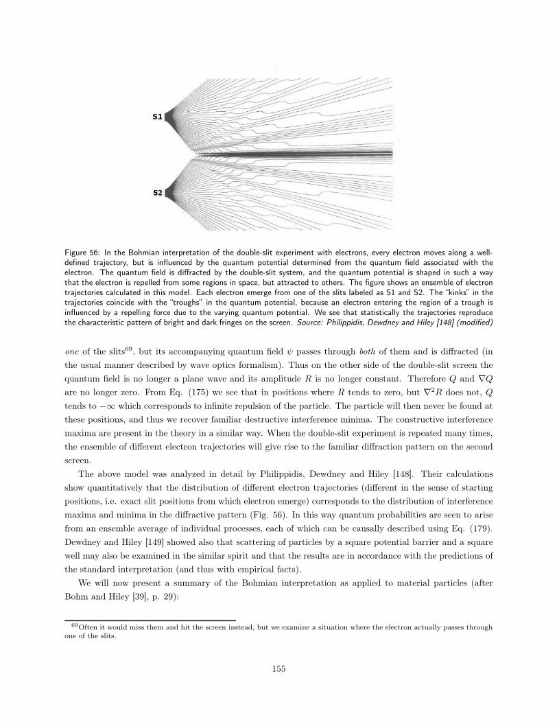
Figure 56: In the Bohmian interpretation of the double-slit experiment with electrons, every electron moves along a well-defined trajectory, but is influenced by the quantum potential determined from the quantum field associated with theelectron. The quantum field is diffracted by the double-slit system, and the quantum potential is shaped in such a waythat the electron is repelled from some regions in space, but attracted to others. The figure shows an ensemble of electrontrajectories calculated in this model. Each electron emerge from one of the slits labeled as S1 and S2. The “kinks” in thetrajectories coincide with the “troughs” in the quantum potential, because an electron entering the region of a trough isinfluenced by a repelling force due to the varying quantum potential. We see that statistically the trajectories reproducethe characteristic pattern of bright and dark fringes on the screen. Source: Philippidis, Dewdney and Hiley [148] (modified)

one of the slits69, but its accompanying quantum field ψ passes through both of them and is diffracted (in

the usual manner described by wave optics formalism). Thus on the other side of the double-slit screen the

quantum field is no longer a plane wave and its amplitude R is no longer constant. Therefore Q and ∇Qare no longer zero. From Eq. (175) we see that in positions where R tends to zero, but ∇2R does not, Q

tends to −∞ which corresponds to infinite repulsion of the particle. The particle will then never be found at

these positions, and thus we recover familiar destructive interference minima. The constructive interference

maxima are present in the theory in a similar way. When the double-slit experiment is repeated many times,

the ensemble of different electron trajectories will give rise to the familiar diffraction pattern on the second

screen.

The above model was analyzed in detail by Philippidis, Dewdney and Hiley [148]. Their calculations

show quantitatively that the distribution of different electron trajectories (different in the sense of starting

positions, i.e. exact slit positions from which electron emerge) corresponds to the distribution of interference

maxima and minima in the diffractive pattern (Fig. 56). In this way quantum probabilities are seen to arise

from an ensemble average of individual processes, each of which can be causally described using Eq. (179).

Dewdney and Hiley [149] showed also that scattering of particles by a square potential barrier and a square

well may also be examined in the similar spirit and that the results are in accordance with the predictions of

the standard interpretation (and thus with empirical facts).

We will now present a summary of the Bohmian interpretation as applied to material particles (after

Bohm and Hiley [39], p. 29):

69Often it would miss them and hit the screen instead, but we examine a situation where the electron actually passes throughone of the slits.

155

1. The massive microscopic particles are corpuscles with well-defined positions. These positions vary

continuously and can be causally determined.

2. Each particle is always accompanied by a new type of quantum field that fundamentally affects it. This

field is described by real variables R(r, t) and S(r, t) satisfying Eq. (176) and (177), or alternatively

by the wave function ψ = ReiS/~ satisfying the Schrödinger equation, Eq. (173). Thus the field also

changes continously and can be causally determined.

3. The particle has an equation of motion given by Eq. (179). The two forces acting on it is the classical

force −∇V (derived from the classical potential V ) and the quantum force −∇Q (derived from the

quantum potential Q which depends on R and is given by Eq. (175)). In the classical limit where

~ → 0 quantum potential may be neglected and we recover the classical equation of motion.

4. The particle momentum is given as p(r, t) = ∇S(r, t). Since the quantum field ψ is single valued, it

can be shown that the following condition applies:

∮

∇S dr =

∮

p dr = nh,

where the integration is conducted along any closed curve in space, and n ∈ N.

5. In a statistical ensemble of particles, selected so that all are characterized by the same quantum field

ψ, the probability density for finding a single particle at a given position and at a given time is

ρ(r, t) = R2(r, t). It should be stressed that the theory is not essentially probabilistic (as in the stan-

dard interpretation), because the statistics merely apply to an ensemble of causally determined particle

trajectories.

9.3.2 The nature of the quantum field

As far as the wave-particle duality problem is concerned, the crucial point of the Bohmian interpretation

is that the movement of massive particles in space is guided by the associated quantum field ψ. While the

particles exhibit solely corpuscular behaviour, the quantum field is responsible for any undulatory (diffractive)

effects that may arise. The main peculiar feature of the quantum field is that its influence depends only on the

form of the field, and not on its amplitude (this is seen directly from the definition of the quantum potential,

Eq. (175), where the amplitude part R of ψ is present both in the numerator and the denominator). Bohm

and Hiley [39] emphasize that the effect of the quantum potential should not be understood mechanically

and that ψ must be interpreted as a kind of information field that steers the movement of an electron.

Furthermore, this steering is of a nonlocal character.

A direct detection of the quantum field proposed by Bohm would of course serve to strengthen his inter-

pretation considerably, but it is actually debatable whether the quantum field possess any energy-momentum

content. If it does, the content is so little that it has so far escaped attention of the experimentalists; if it

does not, the quantum field are impossible to measure directly70. It has been proposed that these waves

could give rise to stimulated emission. Selleri [137] (Chapter 4.3) discussed different experiments aimed at

70Although the lack of any energy content whatsoever would apparently contradict the postulate that the field has informationcontent.

156

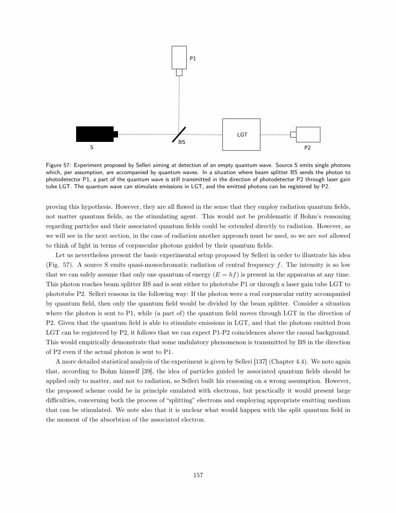
Figure 57: Experiment proposed by Selleri aiming at detection of an empty quantum wave. Source S emits single photonswhich, per assumption, are accompanied by quantum waves. In a situation where beam splitter BS sends the photon tophotodetector P1, a part of the quantum wave is still transmitted in the direction of photodetector P2 through laser gaintube LGT. The quantum wave can stimulate emissions in LGT, and the emitted photons can be registered by P2.

proving this hypothesis. However, they are all flawed in the sense that they employ radiation quantum fields,

not matter quantum fields, as the stimulating agent. This would not be problematic if Bohm’s reasoning

regarding particles and their associated quantum fields could be extended directly to radiation. However, as

we will see in the next section, in the case of radiation another approach must be used, so we are not allowed

to think of light in terms of corpuscular photons guided by their quantum fields.

Let us nevertheless present the basic experimental setup proposed by Selleri in order to illustrate his idea

(Fig. 57). A source S emits quasi-monochromatic radiation of central frequency f . The intensity is so low

that we can safely assume that only one quantum of energy (E = hf) is present in the apparatus at any time.

This photon reaches beam splitter BS and is sent either to phototube P1 or through a laser gain tube LGT to

phototube P2. Selleri reasons in the following way: If the photon were a real corpuscular entity accompanied

by quantum field, then only the quantum field would be divided by the beam splitter. Consider a situation

where the photon is sent to P1, while (a part of) the quantum field moves through LGT in the direction of

P2. Given that the quantum field is able to stimulate emissions in LGT, and that the photons emitted from

LGT can be registered by P2, it follows that we can expect P1-P2 coincidences above the casual background.

This would empirically demonstrate that some undulatory phenomenon is transmitted by BS in the direction

of P2 even if the actual photon is sent to P1.

A more detailed statistical analysis of the experiment is given by Selleri [137] (Chapter 4.4). We note again

that, according to Bohm himself [39], the idea of particles guided by associated quantum fields should be

applied only to matter, and not to radiation, so Selleri built his reasoning on a wrong assumption. However,

the proposed scheme could be in principle emulated with electrons, but practically it would present large

difficulties, concerning both the process of “splitting” electrons and employing appropriate emitting medium

that can be stimulated. We note also that it is unclear what would happen with the split quantum field in

the moment of the absorbtion of the associated electron.

157

9.3.3 Interpretation of electromagnetic field

We have seen how the dual nature of material particles can be explained by the Bohmian interpretation using

the idea of real corpuscles being guided by associated quantum fields (or waves). It is tempting to apply

this explanation directly to the case of radiation, i.e. postulate existence of real massless light corpuscles

(photons) influenced by quantum fields as well. However, Bohm and Hiley [39] (Chapter 11) presented several

reasons that this approach cannot be carried out consistently. Their discussion involves elements of quantum

field theory and we feel that it would be outside of the scope of our text to consider their arguments in

detail. The main difficulty stems from the fact that, using the Klein-Gordon equation as the starting point,

it is difficult, or maybe even impossible, to propose consistent guiding relation which would causally relate

movement of photons to the scalar quantum field.

Bohm and Hiley proposed instead that in electromagnetism the only real physical objects are fields

distributed continuously in space-time. No corpuscular photons actually exist, and any particlelike mani-

festations of these fields must be understood as a result of their nonlocal and nonlinear dynamics. Both

nonlinearity and nonlocality are associated with the so-called super-quantum potential of the field which

becomes negligible in the classical limit (in the similar way as quantum potential from Eq. (175)) where the

fields again obey the classical wave equation.

If we restrict the model to the non-relativistic regime, the mathematical analysis71 is similar to the one

conducted in Section 9.3.1. We introduce wave functional Ψ = Ψ[φ(xµ)] which is dependent on the set

of all field variables φ(xµ) and where we write φ(xµ) instead of φ(r, t). This wave functional can be also

written as:

Ψ = R[φ(xµ)]eiS[φ(xµ)].

From the general form of Schrödinger equation it can be shown that every field variable, say φ1, must obey

a modified wave equation:∂2φ1

∂t2= ∇2φ1 −

δQ

δφ1, (180)

where δδφ1

is the functional derivative with respect to φ1, and Q is the super-quantum potential defined as:

Q = −1

2

∫ δ2

δφ21R

RdV,

where the integration is performed over the whole space.

Bohm and Hiley claimed (without giving any rigorous proof) that it is the presence of the extra term

− δQδφ1

that introduces nonlinear behaviour to the system, but that this term would disappear in the classical

limit where the ordinary wave equation will be recovered. The nonlocality aspect, however, is involved in the

transfer of energy between radiation and matter. For instance, when a wave packet of radiation excites an

atom, energy is “swept in” from the entire wave packet at once as a single quantum of energy.

Thus in the Bohmian interpretation the wave-particle duality of light is no longer paradoxical. Any inter-

ference phenomena can be explained straight-forwardly, since the nature of radiation is de facto completely

undulatory. At the same time any particlelike features are to be understand as the interaction between the

electromagnetic field and matter, and the interaction might be both nonlinear and nonlocal (in the sense

given above). We note that this approach is similar to the semiclassical model of radiation (see Sect. 5.1.2).

71We will use natural constants with ~ = c = 1.

158

We have seen, however, that the semiclassical model of radiation has problems with accomodating results of

some experiments concerned with photocount statistics. In Section 5.1.4 we have discussed the possibility

of introducing effects of perhaps nonlinear character into the semiclassical model. Therefore it would be

very interesting to examine quantitatively whether the model could be improved using the super-quantum

potential idea from the Bohmian interpretation.

9.3.4 Concluding remarks

Two main arguments used by the opponents of the Bohmian interpretation is that it is nonlocal and that it

does not give any new experimental predictions. The nonlocality makes it then untenable on the grounds of

conflict with the relativity theory, while lack of new experimental predictions makes it worthless as a scientific

theory. However, the Bohmian interpretation may be still defended.

It is true that the Bohmian interpretation is explicitly nonlocal, but elements of nonlocality are present in

any present interpretation of the quantum theory, the standard interpretation included. Nonlocality emerges

especially in connection with the EPR paradox and the collapse of the wave function. Other interpretations

are today not able to give a fully local and satisfactory explanation of these phenomena – they are simply less

“frank” about nonlocality than the Bohmian interpretation is. Bohm points out that consistent application of

the nonlocal aspect in his interpretation leads “neither to internal logical contradiction nor to disagreement

with any facts” (Bohm and Hiley [39], p. 157). Furthermore, nonlocal effects become insignifcant in the

macroscopic regime, so the explicit nonlocality does not imply presence of any nonlocal effects that are not

confirmed experimentally. The Bohmian interpretation neither violates special relativity, because its quantum

nonlocality does not allow a signal to be transmitted faster than light.

The second accusation, saying that the Bohmian interpretation does not give any new predictions and

thus cannot be empirically verified, is even more extraneous, because interpretations do not need to give

empirically verifiable predictions. They rather serve to highlight or question some elements of the formalism,

and thus show a possible direction of future research. Strictly speaking, it is the formalism that serves to

predict experimental results, not the interpretation. Both the Copenhagen and the Bohmian approaches have

been showed to give a coherent qualitative description of the quantum-mechanical formalism and its results.

Are there any reasons to favour one of them over the other? The standard interpretation is certainly much

better established today than the Bohmian interpretation, but the reasons are mainly historical, psychological

and sociological. The standard interpretation has been always supported by Niels Bohr’s enormous authority,

while Bohm, during the time when his original papers were published, became somewhat of a scientific outcast

due to political reasons72. However, modern science should show repugnance for the issues of personal

authority, and any interpretation of a physical theory (if several interpretations of the same theory are

possible, as in the case of quantum mechanics) should be judged by its elegance73 and consistence, not by

names attached to it.72In 1949 Bohm was called upon to testify before the House Commitee on Un-American Activites because of his suspected ties

to Communists. He was subsequently arrested and later acquitted, but in the meantime Princeton University had suspendedhim as an assistant professor and after the acquittal the university authorities did not want to renew his contract. Bohm leftfor Brasil, then moved to Israel and finally settled in England. He never returned to United States [150].

73In the sense that as few a priori assumptions should enter it as possible. This is the principle commonly known as Occam’srazor.

159

In the recent times ideas of Bohm have been receiving renewed attention74. Probably it has come together

with the growing realization that the fundamental postulate of the standard interpretation – the denial of

physical reality per se – is a blind alley which suffocates further inquiry into the nature of the physical

world by claiming many interesting questions completely meaningless. On the other hand, the Bohmian

interpretation strives to give a clear intuitive framework within which quantum-mechanical formalism can

be analyzed and further developed. In this task it has already succeeded to some degree. It is most clearly

seen in the case of the wave-particle duality which the interpretation elegantly explains by reducing the

corpuscular and the undulatory behaviour to a common physical principle. It remains to be seen whether the

Bohmian interpretation can be fully extended to the relativistic domain and whether its application will lead

to new formal results that can be confirmed experimentally. If this will happen, the paradigm of quantum

mechanics will doubtlessly change.

74According to the online database at http://prola.aps.org more than 350 scientific papers have referred to Bohm’s originalarticle [144] in the course of last 10 years.

160

10 Conclusion

10.1 Summary and outlooks

In the course of the thesis we have discussed several aspects, both theoretical and experimental, of the wave-

particle duality of light. As remarked already in the Introduction, the duality can be considered from several

angles and thus offers a lot of opportunities for scientific inquiry. Therefore our review had to be limited –

some elements of the problem were discussed in depth, some only mentioned, and some omitted altogether.

However, our presentation of the subject shows clearly that the wave-particle duality can be considered on

three levels.

First and foremost, the duality can be approached directly, as in Chapters 1-3, where we asked how

our perception of light has changed through the last four centuries, what present physical theories support

the undulatory and the corpuscular view, and what experimental evidence supports in turn these different

theories. We have seen that the historical development encourages us to question the contemporary perception

of light. The previous prevailing theories were either overthrown (as Newton’s corpuscular model) or heavily

extended and modified by classical electromagnetism and quantum mechanics (as the Young-Fresnel wave

theory) (Ch. 1). There is no reason to believe that the present paradigm will not change. Multiple questions

regarding the relation between the wavelike and the particlelike behaviour rather suggest that a further

development is inevitable.

From the theoretical point of view there are two main models which encapsulate the undulatory and

the corpuscular view of light. These are, respectively, Maxwell’s electromagnetism (Ch. 2.1) and quantum

mechanics applied to electromagnetic radiation (Ch. 2.3-2.4). While the first one describes light waves in a

very elegant and concise manner, the second one does not manage to do the same for light corpuscles, because

any attempts to localize single photons in space encounter fundamental difficulties (Sect. 2.3.4). Furthermore,

since the radiation field is treated holistically, the distinction between photons and quantized energy content

of the field is rather unclear. These two facts indicate that our present corpuscular theory of light says more

about the interaction between light and matter than about light itself. This is not a disadvantage per se, but in

the context of the wave-particle duality and discussions of “light corpuscles” one should keep this reservation

in mind.

Any physical model should be of course judged by comparing its quantitative predictions with experimental

results, and both theories have had many successes in this respect. The diverse inteference phenomena are

most elegantly explained using the undulatory model (Ch. 3.2). Also, contrary to the widespread belief, the

161

undulatory model is able to account for both photoelectric effect and Compton effect (Ch. 3.3-3.4). The basic

features of these two effects must be therefore dismissed as conclusive empirical confirmation of the photon

hypothesis. Instead of the photoelectric effect and the Compton effect, one should rather refer to correlation

experiments of the type Grangier, Aspect and Roger conducted (Ch. 3.5), because anticoincidence effects

seem to substantiate the corpuscular theory much better. However, we saw that their results could also be

questioned due to the simplifying assumptions involved and the use of nonclassical cascading light source

(see below).

More detailed analysis of the correlation experiments allows us to consider the wave-particle duality on

another level, namely in the context of the photodetection processes and two competing models of photode-

tection – the semiclassical one and the fully quantized one (Ch. 5.1). Obviously, the photodetection process

plays a fundamental role in any situation where the light beam is measured directly. Unfortunately, as far as

statistical properties of light are concerned, the quantum behaviour of classical light cannot be demonstrated

in a satisfying way. We illustrated this fact experimentally and numerically in Chapter 7.1 in the case of

coherent radiation. We saw that it is necessary to employ nonclassical sources of light (i.e. not thermal and

not coherent) in order to obtain experimental results that the semiclassical model cannot account for. But

as we pointed out in Section 5.1.4, the model is somewhat limited by the stationarity condition, so here lies

certain room for its further development.

The semiclassical model could be also improved by putting larger emphasis on fluctuations inherent to

the detectors and through careful analysis of the interactions between light and detectors, especially in the

very low intensity regime (Sect. 5.1.4). The issue of fluctuations was also raised in connection with beam

splitter (Ch. 5.2) during the discussion of the shortcomings of the existing beam splitter models (Sect. 5.2.3).

One should keep in mind that beam splitter is a crucial element of any optical setup aiming at measuring

correlations, so if any hitherto undiscovered effects are present here, they would be able to considerably

influence experimental results.

The theory of coherence presents us with another important aspect of the wave-particle duality. The con-

cepts of coherence length and coherence time may be easily pictured and comprehended in the high intensity

regime using the language of classical electromagnetism. They play a central role in the mathematical de-

scription of fluctuations of chaotic and partially coherent radiation, and they help to explain the emergence of

interference fringes in e.g. double-slit experiments (Ch. 4). However, at very low intensity level it is unclear

how the concept of coherence should be related to the notion of photon. One could for instance assume that

photons are spatially extended and that their size in one way or another corresponds to coherence length,

but then we are effectively replacing light corpuscles with wave packets. On the other hand the notion of co-

herence length cannot be dismissed altogether at very low intensity level, because the interference phenomena

still occurs (Ch. 7.2). It seems that during a further investigation of wave-particle duality one should aim at

establishing an accurate relation between coherence length and the concept of photon (perceived either as a

corpuscle or as an energy quantum of the radiation field).

Finally, there is the third level on which the wave-particle duality can be considered. On this level one

seeks radically new models of light (as Panarella’s photon clump model) or radically new interpretations of

present theories (as Bohm’s interpretation of quantum mechanics) in order to directly reconcile the undulatory

and the corpuscular aspect (Ch. 9). However, this approach requires caution due to its highly speculative

character. We have seen that Panarella’s model implies far-fetched (but nonetheless empirically verifiable)

assumptions about the physical world (Ch. 9.1), while Bohm’s interpretation per definition does not yield

162

any immediate new predictions, although it may stimulate the development of the formalism in some fruitful

direction (Ch. 9.3). At the same time Bohm’s interpretation suggests presence of a nonlinear term in the

wave equation, and such nonlinearity may represent another possibility for improvement of the semiclassical

model.

It is also conceivable that some new experimental setup will challenge the wave-particle duality in its

present form by producing results which none of the present theories is able to account for. We have argued

that Afshar’s experiment does not necessarily produce such results, both because it can be described using

the semiclassical model and because the application of the Greenberger-Yasin inequality (Eq. (170) on p.

135) to the analysis may be questioned (Ch. 8). Nonetheless, Afshar’s experiment remains a very clever

nonperturbative measurement scheme with possible future applications.

It is rather obvious that our whole discussion of the wave-particle duality has been slanted towards the

undulatory view of light. This is not due to any prejudice present from the outset, but rather from the fact

that the particlelike properties, after closer inspection, seem much more elusive than the wavelike properties.

We notice that while nonclassical sources of light are needed in order for radiation to exhibit corpuscular

behaviour (in the sense of photocount statistics as discussed above), the undulatory behaviour is present for

both classical and nonclassical sources at any level of intensity, also in the very low intensity regime usually

interpreted as "the single photon level". It seems therefore that if one of the models might be made redundant,

the corpuscular properties could be embedded into the wave theory, but not the other way around. In the

author’s opinion future inquiries into the wave-particle duality problem should be connected with attempts

to extend the semiclassical model beyond its present boundaries, both through a closer examination of the

stationarity condition and through introducing additional (possibly nonlinear) effects into the semiclassical

theory of photodetection.

On the basis of his work the author would now like to propose the following prospects:

• More detailed theoretical analysis of the difficulties that arise when we try to describe photon localiza-

tion using wave function formalism. We touched briefly upon this subject in Sect. 2.3.4, but it deserves

surely further examination.

• Closer analysis of the notion of coherence in the very low intensity regime. Especially one could try

to construct models which associate coherence directly with the photonic entity and which perhaps

predict that coherence length is dependent in a specific way on the number density of photons in the

beam. Such predictions could be then tested experimentally.

• Conduct of a photomeasuring experiment with a classic light source which yields statistical results

conflicting the predictions of the semiclassical model in its standard form. Such an experiment has

been proposed in Sect. 5.1.4. The semiclassical model could then be appropriately extended in order

to account for the results, and this extension could be in turn applied to nonclassical sources in order

to see whether their emission can be described without refering to the fully quantized model.

• Development of new beam splitter models along the lines proposed in Sect. 5.2.3.

• Further development of the numerical routine presented in Appendix D which can be employed to

simulate correlation measurements. More complex beam splitter and photodetection models could be

incorporated into the routine and simulations based on diverse assumptions could be then performed,

163

both in order to gain better insight into different possibilities, and in order to test different hypotheses

and compare their predictions with experimental results.

• Combining Afshar’s experiment with Grangier, Roger and Aspect’s correlation experiment in order to

create an experimental setup where both the nonperturbative measurement of interference pattern and

the anticoincidence effect observed by Grangier et al. are present at the same time.

• Explicit testing of the predictions given by Panarella’s photon clump model.

• Theoretical development of Bohm’s idea regarding the possible presence of nonlinear terms in equations

governing the undulations of electromagnetic field. This nonlinearity could be used in order to extend

the semiclassical model.

10.2 Closing words

Does the wave-particle duality deserves an explanation? Or, more precisely, should physicists seek a more

general model of light from which the undulatory properties and the corpuscular properties emerge naturally?

Or should we rather develop further the existing, mutually exclusive models, and do not attempt to build

a bridge between them, unless future research will suggest in a direct way how such a connection could be

constructed? The answers to these questions are heavily conditioned by one’s approach to the science of

physics in general. There are two main motivations for studying, doing and applying physics to the broad

array of natural phenomena. In most cases these motivations are “superposed”, but sometimes one dominates

over the other, so it is easy to distill them in their pure forms.

The first motivation stems from our will to comprehend the world and the observable processes ontolog-

ically, through establishing as close correspondence as possible between our physical models and different

aspects of reality. The correspondence can be never made complete, so there may easily occur a situation

where the same aspect of reality is described by different models yielding correct quantitative predictions.

However, one should then endeavor to attain a maximal degree of consistency between models in order to

create as coherent picture of reality as possible. In this approach the qualitative plane seems superior to

the quantitative one. Of course, the mathematical apparatus is indispensable as a methodological tool that

makes us capable of verifying individual models by confronting their predictions with experimental results,

but the ability to perform correct calculations and to quanitatively anticipate phenomena does not have any

particular significance on its own.

With this approach to physics the need for an unambiguous clarification of the wave-particle duality

is obvious. We want "only" to answer precisely the question about the nature of electromagnetic radiation

without making use of the complementarity notion, because the claim that light sometimes behaves as a wave,

and sometimes as a corpuscle, and that there is no deeper level of reality on which these two manifestations

could be merged – such claim seems very unsatisfying. Of course, "unsatisfying" does not imply "untrue",

but the history of physics has showed us so far that there are answers for almost any question, even though

these answers eventually lead to new questions.

The second motivation for working with physics is of a calculational character. Physicists impelled by

it want primarily to apply mathematical tools to natural phenomena in order to model them quantitatively,

164

and questions about the nature of reality (in the sense of looking for concise and fully consistent qualitative

descriptions) are for them of secondary importance. Thus, this doctrine is rather phenomenological or

epistemological than ontological. According to it the aim of physical models is to simulate natural phenomena.

Any ambitions of emulating the reality must be given up. This simulative and more reserved approach was

succintly (and probably half-jokingly) expressed by David Mermin in his oft-quouted declaration: "If I were

forced to sum up in one sentence what the Copenhagen interpretation says to me, it would be ’Shut up and

calculate!’" [151]. The calculational attitude suggests that deliberation on the "true" meaning of theories and

search for new interpretations of prevailing formalisms at some point should be simply ceased, and thereafter

the only thing that counts is the ability to perform precise, empirically confirmed calculations.

Within this strategy the need for explaining the wave-particle duality is much less obvious. The calcu-

lational approach suggests that instead of struggling with the question on the nature of light, a physicist

should focus his or her efforts on mathematical descriptions of phenomena in which light is involved. If results

were to suggest an unequivocal qualitative interpretation, one should of course embrace it, but if no such

interpretation were to appear, one should not consider it as a problem that physics must overcome. After all,

employing several different models of electromagnetic radiation is not troubling from the calculational point

of view, as long as each of these models yields correct results within its applicability range, and as long as

no new phenomena are discovered that none of the models is able to explain.

Let us, however, notice two things. First of all, attempts at unificating different models have been one

of the main drives for the development of physics, since new theories often are born on boundaries between

the old ones. The phenomena of electricity and magnetism were fused by Maxwell’s electromagnetism; when

trying to explain incosistencies between electromagnetism and classical mechanics Einstein worked out the

special theory of relativity; and then, while incorporating Newton’s theory of gravity into the latter, Einstein

developed the general theory of relativity. Thus we see that in any situation where several competing physical

models are present, there lies a possiblity for unification, and unifications always lead to new and sometimes

astonishing results.

Secondly, even if we are impelled by the first (emulative) motivation when searching for a new model,

we will be guided by the methodology intimately connected with the second (simulative) motivation – which

confronts predictions of temporary hypotheses with experimental results. In other words, if we at some

time in the future achieve our goal and find a model that elegantly answers our qualitative questions about

natural phenomena, the model will necessarily be correct from the empirical point of view (because otherwise

it would be scientifically worthless), and thus can be employed in a purely quantitative manner. Therefore

the advocates of the calculational approach will also greatly benefit from it, especially if the model makes

use of more elegant and sharper mathematical methods.

We stress again that in practice both motivations are usually blended, as in the case of the author

when working with the above thesis. Investigating the problem of the wave-particle duality presents us with

an excellent opportunity for asking many exciting questions regarding the nature of the light, our way of

perceiving and measuring it, the limits of our current models and our interpretations of physical theories.

On the other hand, this type of inquiry serves at the very least to clarify the existing models – but possibly

may also lead to development of new and fruitful ones.

As a final side note, we notice an interesting parallel. When modern physics was born in the 17th century,

two crucial questions were posed regarding the nature of the world: "What is gravity?" and "What is light?".

Newton admitted that he was not able to explain how physical bodies influence each other through vast

165

cosmic distances. The "essence" of gravitational interactions remained a mystery for several centuries, until

Einstein presented his very elegant theory which interpreted gravitation as space-time curvature. The general

theory of relativity led to many new questions within the cosmological framework, but today the geometrical

view of gravity itself stands very strongly.

The question about the nature of light, however, led rather quickly to two conflicting answers, and this

conflict has survived to the present day. The opposing views of light have gone far along their respective

paths, but they have not been reconciled by any conceptual breakthrough comparable to that associated

with Einstein’s relativity. In the recent years it seems that these two paths finally started to converge, due

to technological progress represented by laser, nonclassical sources of light and modern detectors, and due to

new physical theories as quantum optics and quantum electrodynamics. It is the author’s hope that the near

future will show whether the convergence can be made complete and whether the notion of wave-particle

duality will become as anachronistic as that of luminiferous aether that light had once been believed to

propagate through.

Borys JagielskiOslo, 28.05.2009

166

A The formalism of quantum mechanics

The wave-particle duality is deeply rooted in the quantum mechanics. In the author’s opinion, however, it

would be exorbitant to dedicate a separate chapter to the basic notions of the quantum-mechanical formalism,

since they are assumed to be well-known to the reader. Nonetheless, throghout the thesis, we refer to

some particular (although still fundamental) relations incorporated in the theory. Therefore, for the sake of

completeness, we present here in a highly abbreviated form the basic formalism of the quantum mechanics.

Our focus is on the postulates, on the essential results related to the measurement theory and on Heisenberg’s

uncertainty principle (the full proof of which is included). For a more detailed and very readable formal

introduction to quantum mechanics (which does not refrain from discussing several subtle points usually

omitted by other authors) we refer to Isham [152]. A standard modern reference to the subject is Shankar

[51].

The mathematical apparatus of quantum mechanics and its linkage to the physical world rest on the four

following postulates:

1. Each physical state is represented by a (normalized) time-dependent vector |Ψ〉 belonging to a complex

Hilbert space75 H. The complex Hilbert space forms the state space of the physical system.

2. Each measurable physical quantity A, called an observable, is represented by a self-adjoint76 (i.e.

Hermitian) operator A acting on the vectors in the complex Hilbert space.

3. Given an ensemble of identical physical states, each represented by a normalized vector |Ψ〉 ∈ H, the

mean measured value of A is the scalar product of |Ψ〉 with A |Ψ〉. Using Dirac’s notation77 we write

〈A〉 = 〈Ψ| A |Ψ〉 . (181)

4. The time evolution of any closed (isolated) system is described by a differential equation called

Schrödinger’s equation:

i~d |Ψ(t)〉dt

= H |Ψ(t)〉 , (182)

75A complex Hilbert space is a complex inner product space that is complete under the norm defined by the inner product.Completeness means that every Cauchy sequence of vectors in the space has a limit that also belongs to the space.

76Self-adjointness of an operator A means that the operator is equal to its conjugate transpose, A† = A.77In this notation the scalar product of a vector |x〉 with a vector |y〉 is written as 〈x|y〉 = 〈y|x〉∗.

167

where ~ is Planck’s constant divided by 2π, and H is the Hamiltonian operator, an operator formed

from the classical Hamiltonian of the system. Here we have written |Ψ(t)〉 instead of |Ψ〉 in order to

stress the time-dependency of the vector.

It can be shown that all eigenvalues of any Hermitian operator A are real, and that the eigenvectors |φi〉belonging78 to these eigenvalues form an orthogonal and complete79 set. Orthogonality implies 〈φi|φj〉 = 0 if

i 6= j, and because of the completeness any vector |Ψ〉 belonging to a finite-dimensional H can be expressed

as a linear combination of the orthonormalized eigenvectors of any Hermitian operator A:

|Ψ〉 =N∑

i=1

ci

∣

∣

∣φ

′

i

⟩

,

whereN is the total number of eigenvectors (or, equivalently, the dimensionality of the Hilbert space involved),

ci is a complex coefficient calculated from ci = 〈φi|Ψ〉 (this relation follows from the orthogonality of the

eigenvectors), and∣

∣

∣φ

′

i

⟩

is the normalized |φi〉:

∣

∣

∣φ

′

i

⟩

=|φi〉

√

〈φi|φi〉.

A crucial result can be derived from Rule 3. If, given a physical state described by |Ψ〉, we perform

a measurement of an observable A, the measurement will always80 yield one of the eigenvalues of A. The

probability of the measurement resulting in some non-degenerate eigenvalue is simply |ci|2 = |〈φi|Ψ〉|2 where

|φi〉 is the associated eigenvector. If, however, the asked-for eigenvalue is degenerate, we have to sum |〈φi|Ψ〉|2

over all associated eigenvectors |φi〉.The above result is fundamental for the quantum-mechanical measurement theory, and it shows how the

probabilistic nature of the theory comes about. We emphasize that it is not an additional postulate, but it

follows from Rule 3; alternatively, Rule 3 can be derived from it, so this result is sometimes presented as its

equivalent version. However, both possible forms of Rule 3 have to be supplied by another (experimentally

verifiable) postulate: The act of measurement leads to an instantaneous change of the quantum state from

|Ψ〉 to |φi〉, where |φi〉 is the eigenvector associated with the eigenvalue which the measurement has yielded.

This phenomenon is called the collapse of the wave function81.

We notice that the possibility of the collapse is altogether absent from Schrödinger’s equation, Eq. (182).

The equation describes the deterministic time evolution of |Ψ〉 until a measurement is made. Then the evolved

state collapses to one of the eigenvectors of the operator associated with the measured observable, and the

time evolution continues, again in accordance with Schrödinger’s equation, until the next measurement is

made, and so on. In other words, the time evolution of a quantum state consists of two parts: the deterministic

and continuous part described fully by Schrödinger’s equation, and the probabilistic and non-continuous part

78The number of distinct eigenvalues may be smaller than the number of distinct (i.e. linearly independent) eigenvectors.In such a situation at least two distinct eigenvectors share the same eigenvalue, and we say that the (eigen)spectrum of theoperator is degenerate.

79The completeness of the eigenvectors is not to be confused with the completeness of the Hilbert space. Furthermore weimplicitly assume that the considered is finite-dimensional. The argument can be extended to infinite-dimensional vector spacesas well, but then some additional aspects of the formalism must be discussed. The original reference is Dirac [153].

80Given the measurement is ideal, i.e. as precise as theoretically possible.81If the eigenvalue is degenerate, the vector collapses to a superposition of the associated eigenvectors. The eigenvectors in

the superposition are weighted as in the original vector.

168

associated with the act of measurement.

We notice that Eq. (182), as written above, is formally problematic, because it is not clear what one

means with the time derivative of a vector. We should rather express it as:

i~∂ψ(q, t)

∂t= 〈q| H |Ψ(t)〉 , (183)

where ψ(q, t) ≡ 〈q|Ψ(t)〉 is the coordinate representation of |Ψ(t)〉, and |q〉 is an eigenvector associated with

an eigenvalue q of the coordinate observable q. The most usual coordinate representations are those given

by position x or momentum p. Their eigenspectra are continuous. If we work in the position representation,

the position variable x is represented simply as x, but according to the standard prescription the momentum

variable is represented as a differential operator, p → −i~ ∂∂x . Thus the Hamiltonian for a free particle,

H = p2

2m +V (x) (with m being the mass of the particle and V the position-dependent potential), becomes in

the position representation the operator H = −~2

2m

(

∂∂x

)2+ V (x). Schrödinger’s equation for such a particle

yields:

i~∂ψ(x, t)

∂t=

−~2

2m

∂2ψ(x, t)

∂x2+ V (x)ψ(x, t).

Since the proper form of Schrödinger’s equation, Eq. (183), is valid in any coordinate representation, it is

justifiable to use the more compact version given by Eq. (182).

A central axiom of the quantum theory is that the position and momentum operators do not commute:

xpx − pxx ≡ [x, px] = i~, (184)

with the lower index x standing for the x-component of the momentum. In three dimensions we have:

[ri, pj ] = i~δij , i, j = x, y, z. (185)

One can prove that two Hermitian operators have the same set of eigenfuctions if and only if they commute. In

physical terms this is interpreted as the claim that we are principially unable to measure simultaneously two

non-commuting observables of a physical system with an arbitrarily large precision. One of the measurements

will inevitably disturb the physical system and influence the outcome of the second measurement. If the first

observable is measured with full precision, the disturbance of the value of the second observable will be

maximal in the sense that uncertainty in the second measurement will be infinitely large.

It should be stressed that the last two sentences of the previous paragraph take for granted the realistic

stance. By using the phrase “the disturbance of the value of the second observable” we have assumed that

the formalism of quantum mechanics describes a physical reality, and that a quantity associated with a

physical system has some value even before the actual measurement of that value is being made. Such a

realistic approach is intuitively obvious, but in fact it is denied by the Copenhagen interpretation of quantum

mechanics. We have elaborated on this point in Chapter 9.2.

Apart from the problem of choosing an appropriate interpretation, the uncertainty associated with mea-

suring two non-commuting observables is quantified by the ubiquitous Heisenberg’s principle. We end this

appendix by demonstrating its generalized version. We follow the proof given by Griffiths [154] (pp. 110-111).

Rule 3 gives the formula for calculating the mean value of an observable A given a system described by

|Ψ〉:〈A〉 = 〈Ψ|A|Ψ〉 ≡ µA.

169

The variance σ2A (the spread of the results about 〈A〉) is:

σ2A ≡

⟨

(A− µA)2⟩

= 〈Ψ|(

A− µA

)2

|Ψ〉 = 〈Ψ|(

A− µ)† (

A− µA

)

|Ψ〉, (186)

where the last equality is allowed because A (and thus A−µ, since µ is a real scalar) is Hermitian. We define

a new vector state:

|α〉 ≡(

A− µA

)

|Ψ〉 ,

and so:

σ2A = 〈α|α〉.

For any other observable B we thus have:

σ2B = 〈β|β〉,

with |β〉 ≡(

B − µB

)

|Ψ〉 and µB ≡ 〈Ψ|B|Ψ〉. Now, from the Schwarz inequality [155] it follows that:

σ2Aσ

2B = 〈α|α〉〈β|β〉 ≥ |〈α|β〉|2,

which is valid for any two observables A and B. Since the scalar product 〈α|β〉 is a complex number z, and

since for any complex number it is true that:

|z|2 = ℜ(z)2 + ℑ(z)2 ≥ ℑ(z)2 =

[

1

2i(z − z∗)

]2

,

we have:

σ2Aσ

2B ≥

[

1

2i(〈α|β〉 − 〈β|α〉)

]2

. (187)

Now we calculate 〈α|β〉 explicitly:

〈α|β〉 = 〈Ψ|(

A− µA

)† (B − µB

)

|Ψ〉 = 〈Ψ|(

A− µA

)(

B − µB

)

|Ψ〉 =

〈Ψ|AB|Ψ〉 − µB 〈Ψ| A |Ψ〉 − µA 〈Ψ| B |Ψ〉 + µAµB〈Ψ|Ψ〉 =

〈Ψ|AB|Ψ〉 − µBµA − µAµB + µAµB = 〈AB〉 − µAµB ≡ µAB − µAµB,

where µAB ≡ 〈AB〉. Similarly we get 〈β|α〉 = µBA − µAµB with µBA ≡ 〈BA〉. Thus:

〈α|β〉 − 〈β|α〉 = µAB − µBA = 〈Ψ|(

AB − BA)

|Ψ〉 = 〈Ψ|[

A, B]

|Ψ〉 =⟨[

A, B]⟩

.

If we insert the above result back into Eq. (187), we get the generalized uncertainty principle which gives us

the lower bound for the product of two variances of two observables:

σ2Aσ

2B ≥

[

1

2i

⟨[

A, B]⟩

]2

. (188)

It follows that if the operators associated with the two observables commute, then the lower bound is zero. If

the two observables, however, are position x and the x-component of momentum px, Eq. (188) yields (with

170

the help of the canonical commutation relation, Eq. (184)):

σ2xσ

2px

≥[

1

2i〈[x, px]〉

]2

=

[

1

2i〈i~〉

]2

=~

2

4,

so:

σxσpx≡ (∆x) (∆px) ≥ ~

2.

Using Eq. (185) we readily obtain a three-dimensional generalization:

(∆x)(∆y)(∆z) (∆px) (∆py) (∆pz) ≥~3

8≈ ~

3. (189)

171

172

B Demonstration of properties of the coherent states

In the following we will prove the properties of the coherent states listed in Chapter 2.4. Our treatment

is guided by Leinaas [156] (Chapter 1) and Mandel and Wolf [55] (Chapter 11).

B.1 The minimal uncertainty

We are going to prove that the coherent states |z〉 are the minimal uncertainty states, i.e. that for all z

Heisenberg’s uncertainty principle becomes an equality:

√

〈z| (∆q)2 |z〉√

〈z| (∆p)2 |z〉 =~

2. (190)

Here (∆q)2 is the dispersion operator for the coordinate operator q. The dispersion operator is defined as:

(∆q)2 ≡ (q − µq)

2, (191)

with:

µq ≡ 〈z| q |z〉 (192)

being the mean value of the coordinate q. Similarly, (∆p)2 is the dispersion operator for the conjugate

momentum operator p. As noticed in Appendix A, the mean dispersion is simply the variance of the related

observable (cf. Eq. (186)).

From Eqs. (191)-(192) we see that:

〈z| (∆q)2 |z〉 = 〈z| q2 |z〉 − 〈z| q |z〉2 . (193)

A similar relation holds for 〈z| (∆p)2 |z〉. Furthermore, in Eqs. (17)-(18) in Chapter 2.2 we have seen how

the annihilation and creation operators (then called the lowering and the raising operators) are defined in

the case of a massive harmonic oscillator. In the case of electromagnetic field these definitions are almost

identical, but since the photons are massless the mass is absent. Thus we have:

a ≡√

ω

2~

(

q +i

mωp

)

a† =

√

ω

2~

(

q − i

mωp

)

,

173

where ω is the angular mode frequency. It follows that:

q =

√

~

2ω

(

a† + a)

p = i

√

~ω

2

(

a† − a)

.

The formula for q gives us:

q2 =~

2ω

(

a†2 + a2 + a†a+ aa†)

=~

2ω

(

a†2 + a2 + 2a†a+ 1)

where we have used the commutation relation from Eq. (41) (Ch. 2.3.3) Using the above expression together

with the defining eigenvalue relation for the coherent states (Eq. (52), Ch. 2.4), Eq. (193) readily yields:

〈z| (∆q)2 |z〉 =~

2ω

(

z∗2 + z2 + 2z∗z + 1)

− ~

2ω

(

z∗2 + z2 + 2z∗z)

=~

2ω.

Along the same lines one could show that:

〈z| (∆p)2 |z〉 =~ω

2.

The minimal uncertainty relation that we have set out to prove, Eq. (190), follows at once.

B.2 The time evolution of a coherent state

We examine how an arbitrary coherent state |z〉 evolves in time. We choose to work in the Heisenberg

picture, so let us equip the annihilation operator a with time-dependency according to the standard quantum

mechanical formula:

a(t) = U(t)†aU(t), (194)

where U(t) is the time operator:

U(t) = e−i~

Ht,

with H being the Hamilton operator. Thus, using Eq. (23) (Ch. 2.2) we see that U(t) = e−iω(a†a+ 12 )t and

from Eq. (194) we get

a(t) = eiωta†aae−iωta†a (195)

after the 12 -factors have been cancelled. Now, the operator expansion theorem states that for any two

operators A and B [157]:

exABe−xA = B + x[A, B] +x

2![A, [A, B]] + ...

An important lemma follows immediately:

eABe−A = B + [A, B] +1

2![A, [A, B]] + ... (196)

174

With its help Eq. (195) can be simplified to:

a(t) = e−iωta.

Now let us apply the time evolution operator to a coherent state |z〉 and operate with a on top of that.

a(U(t) |z〉) = U(t)(U(t)†aU(t)) |z〉 = U(t)a(t) |z〉 = U(t)(e−iωta) |z〉 =

U(t)(e−iωtz) |z〉 = e−iωtz(U(t) |z〉)

If we define |z(t)〉 ≡ U(t) |z〉, we see that a |z(t)〉 = z(t) |z(t)〉 with z(t) = e−iωtz. The coherent state

evolves with time into other coherent states, and the original eigenvalue z simply gets a revolving phase factor

e−iωt. Thus the time evolution is periodic with period 2πω . It follows that the uncertainty examined in the

previous section is always minimal.

B.3 The coherent states as a basis

We demonstrate now that the coherent states form a basis for the representation of arbitrary quantum

states, but a basis that is non-orthogonal and over-complete (in the sense soon to be explained). We begin the

proof with introducing the displacement (shift) operator D(z) which may be used to generate an arbitrary

coherent state from the ground state |0〉. It is defined as:

D(z) = eza†−z∗a, (197)

so that:

D†(z) = ez∗a−za†

.

From the algebraic formula [157]:

eAeB = eBeAe[A, B], if [A, [A, B]] = [B, [A, B]] (198)

and from the commutation relation Eq. (19) (Ch. 2.2) it follows that D(z)D†(z) = 1, so the displacement

operator is unitary.

Now use the displacement operator to unitary transform the annihilation and creation operator:

D†(z)aD(z) = ez∗a−za†

aeza†−z∗a = a+ z1

D†(z)a†D(z) = ez∗a−za†

aeza†−z∗a = a† + z∗1.

The lemma from Eq. (196) has been employed. We see now that D(z) is effectively able to shift the ground

state to an arbitrary coherent state:

a(D(z) |0〉) = (D(z)D†(z))a(D(z) |0〉) = D(z)(D†(z)aD(z)) |0〉) =

= D(z)(a+ z1) |0〉 = zD(z) |0〉 ,

175

Thus we obtain the following expression for an arbitrary coherent state |z〉:

|z〉 = D(z) |0〉 .

We now have to examine the wave function of a number state in the coherent state representation,

ϕn(z) ≡ 〈z|n〉 = 〈n|z〉∗. First we state the Campbell-Baker-Hausdorff formula which is again valid for any

two operators A and B whose commutator [A, B] commutes with both A and B [157]:

ex(A+B) = exAexBe−x2[A, B]/2 = exBexAex2[A, B]/2. (199)

Now we are in position to calculate 〈n|z〉:

〈n|z〉 = 〈n|D(z)|0〉 = 〈n|eza†−z∗a|0〉 = 〈n|e− 12 |z|

2

eza†

e−z∗a|0〉 =

e−12 |z|

2〈n|∞∑

j=0

zj

j!(a†)j

∞∑

k=0

(−z∗)k

k!ak|0〉 = e−

12 |z|

2〈n|∞∑

j=0

zj

j!(a†)j |0〉 = e−

12 |z|

2 zn

√n!. (200)

Here we have made use of, respectively, Eq. (199), the fact that a |0〉 = 0, and Eq. (20). Thus we have:

ϕn(z) ≡ 〈z|n〉 = 〈n|z〉∗ = e−12 |z|

2 (z∗)n

√n!

(201)

The probability distribution for having n photons in the coherent state as a function of the complex

variable z is given by the absolute square of ϕn(z):

|ϕn(z)|2 = e−|z|2 |z|2n

n!.

Since the expectation value of the number of photons in the coherent state |z〉 is simply:

〈n〉 = 〈z|n|z〉 =⟨

z|a†a|z⟩

= |z|2,

we observe that the probability distribution for having n photons in the coherent state is Poissonian:

P|z〉(n) = e−〈n〉 〈n〉n

n!(202)

Let us also notice that the alternative definition of the coherent states, Eq. (51) (Ch. 2.4), follows easily

from Eq. (200) supplemented by Eq. (21) (Ch. 2.2):

|z〉 =

∞∑

n=0

|n〉 〈n|z〉 =

∞∑

n=0

e−12 |z|

2 zn

√n!

|n〉 .

We are now ready to complete the proof and show that the coherent states form a non-orthogonal and

over-complete basis. We are going to use the completeness of the number states (Eq. (21)) and Eq. (201).

176

We consider the scalar product of two different coherent states called |z〉 and |z0〉:

〈z|z0〉 =∑

n

〈z|n〉 〈n|z0〉 =∑

n

e−12 |z|

2 (z∗)n

√n!e−

12 |z0|2 (z0)

n

√n!

=

= e−12 (|z|2+|z0|2)

∑

n

(z∗z0)n

n!= e−

12 (|z|2+|z0|2+z∗z0). (203)

Absolute squaring gives

|〈z|z0〉|2 = e−12 |z−z0|2 .

Thus we see that the two different coherent states are not orthogonal. However, the modulus of their inner

product converges quickly to zero if the difference between z and z0 is significant.

We finally show that the coherent states form an over-complete basis. We do it by verifying the com-

pleteness relation directly. Since z is a continuous variable, the summation from Eq. (21) has to be replaced

by integration over all possible z:

∫

d2z |z〉 〈z| =

∫

d2z∑

m, n

|m〉 〈m|z〉 〈z|n〉 〈n| =

∫

d2z∑

m, n

|m〉 e−|z|2 zm(z∗)n

√m!n!

〈n|

We have employed Eq. (201). Now, by switching to polar coordinates and utilizing the fact that zm = rmeimθ

where r ≡ |z| and θ = arg(z), we obtain

∫

d2z |z〉 〈z| =∑

m, n

|m〉 〈n|√m!n!

∫ ∞

0

dr rm+n+1e−r2

∫ 2π

0

dθ ei(m−n)θ =

=∑

m, n

|m〉 〈n|√m!n!

∫ ∞

0

dr rm+n+1e−r2

2πδmn =

= 2π∑

n

|n〉 〈n|n!

∫ ∞

0

dr r2n+1e−r2

= 2π∑

n

|n〉 〈n|n!

1

2n! = π1

where we have used the definition of the Γ-function and its relation to the factorial:

Γ(s) =

∫ ∞

0

rs−1e−r dr

Γ(s) = (s− 1)!, when s ∈ N

Thus we conclude that the coherent states fulfill the relation:

1

π

∫

d2z |z〉 〈z| = 1. (204)

We have shown that the coherent states form a non-orthogonal and over-complete basis. Over-completeness

implies that any coherent state can be expressed in terms of other coherent states. Using Eqs. (203) and

(204) we immediately obtain for an arbitrary coherent state |z〉:

|z〉 = 1 |z〉 =1

π

∫

|z′〉 〈z′| z〉 d2z =1

π

∫

e−12 (|z|2+|z′ |2+z

′∗z) |z′〉 d2z.

177

It was demonstrated by Cahill [158] that the set of coherent states cannot be made exactly complete

by substracting from it a countable number of elements. On the other hand, the over-completeness of the

coherent states is mathematically a very desirable property, because a coherent-state representation of an

arbitrary quantum state |Ψ〉 is completely determined by coefficients 〈z|Ψ〉 within some arbitrarily (but not

infitesimally) small range of z. Furthermore, a coherent-state representation of any traceable, positive definite

Hermitian operator A is completely determined by its diagonal matrix elements 〈z| A |z〉 again within some

arbitrarily (but not infitesimally) small range of z. These two properties are proved and discussed at length

in Mandel and Wolf [55] (Chapters 11.6-11.7).

178

C Matter waves

As explained in Introduction, the wave-particle duality is commonly associated with both light and matter,

but in the thesis our attention has been restricted to light only. However, in several places (Chapter 3.4

and Chapter 9.3) we are nonetheless forced to refer to the duality of matter. Therefore, for the sake of

completeness, in the following appendix we give a strongly abbreviated presentation of the subject, both

from the theoretical and from the experimental side.

It was the French physicist and nobleman Louis de Broglie who in his doctoral thesis in 1924 presented

the revolutionary idea that all matter had a wavelike nature. This conceptual breakthrough, confirmed in an

electron diffraction experiment due to Lester Germer and Clinton Davisson three years later, paved way for

the further development of quantum mechanics in the late 20s and the 30s. The so-called de Broglie relations,

put in a very simple but strictly mathematical form, assign to every physical particle (like an electron) a

wavelength and a frequency. These parameters can then be used to anticipate and describe the diffractive

behaviour of the particles.

The basic postulate is this: Given a physical object with momentum p and total energy E, we relate to

it a wavelength λ and a frequency f given by the formulas [36]:

λ =h

p(205)

f =E

h. (206)

The relativistic effects could be taken into account by introducing the Lorentz factor, γ = 1/√

1 − v2

c2 , and

setting p = γmv and E = γmc2.

It is not immediately clear what is meant by “relating wavelength and frequency to a physical object”.

We have seen in Chapter 9.2 that within the Copehnagen interpretation of quantum mechanics one simply

perceives physical objects themselves as undulatory phenomena (in specific experimental circumstances),

while Bohm’s interpretation (see Ch. 9.3) claims that particles are always accompanied by quantum fields

responsible for their undulatory behaviour.

It is instructive to consider a simple numerical example. An electron with mass me = 9.11×10−31 kg and

moving with 10% of the speed of light, v = 0.1c, has wavelength λ = 2.4× 10−11 m which is comparable with

the size of an atom (≈ 10−10 m). Thus, a slowly moving electron will be able to show a diffractive behaviour

while interacting with matter. On the other hand a car with mass, say, m = 1000 kg and moving with speed

v = 100 km/h ≈ 28 m/s has wavelength λ = 2.4 × 10−38 m which is three orders of magnitude smaller than

179

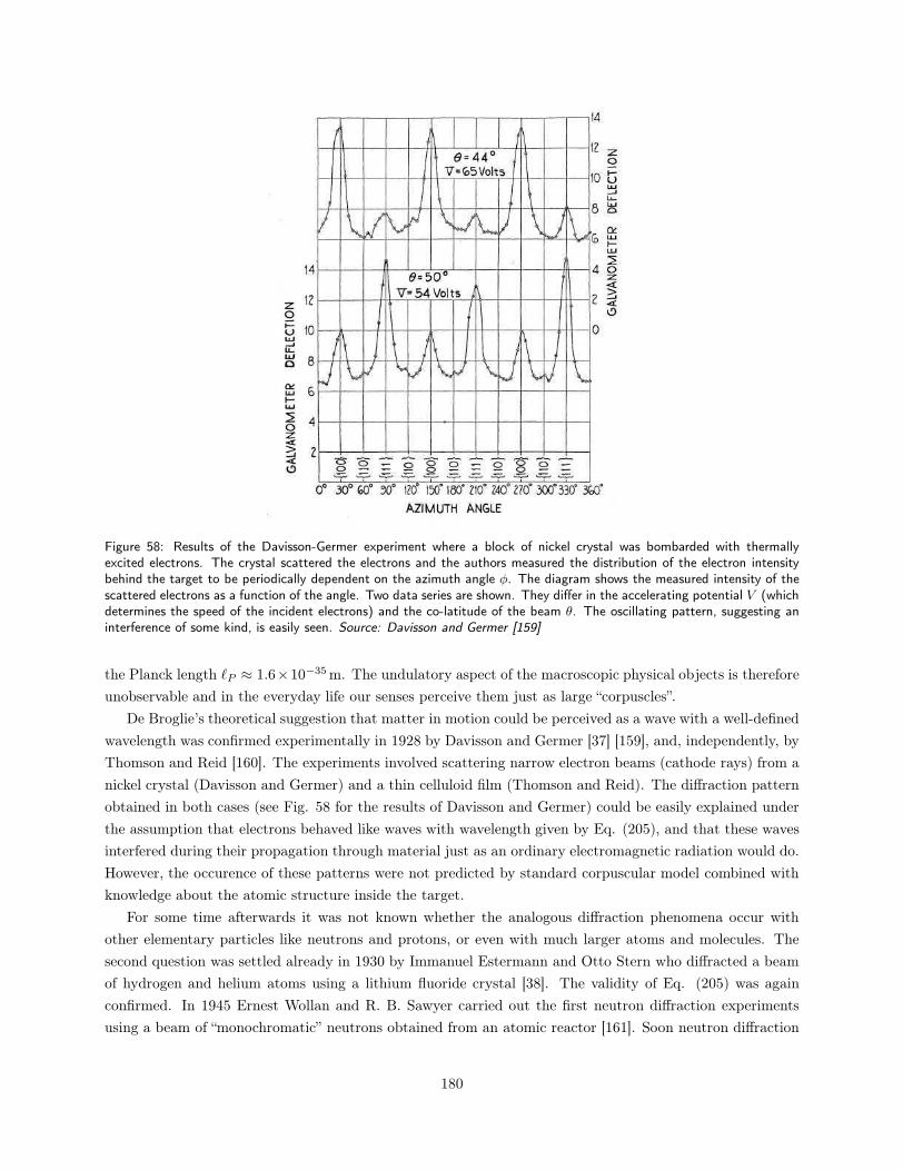
Figure 58: Results of the Davisson-Germer experiment where a block of nickel crystal was bombarded with thermallyexcited electrons. The crystal scattered the electrons and the authors measured the distribution of the electron intensitybehind the target to be periodically dependent on the azimuth angle φ. The diagram shows the measured intensity of thescattered electrons as a function of the angle. Two data series are shown. They differ in the accelerating potential V (whichdetermines the speed of the incident electrons) and the co-latitude of the beam θ. The oscillating pattern, suggesting aninterference of some kind, is easily seen. Source: Davisson and Germer [159]

the Planck length ℓP ≈ 1.6×10−35 m. The undulatory aspect of the macroscopic physical objects is therefore

unobservable and in the everyday life our senses perceive them just as large “corpuscles”.

De Broglie’s theoretical suggestion that matter in motion could be perceived as a wave with a well-defined

wavelength was confirmed experimentally in 1928 by Davisson and Germer [37] [159], and, independently, by

Thomson and Reid [160]. The experiments involved scattering narrow electron beams (cathode rays) from a

nickel crystal (Davisson and Germer) and a thin celluloid film (Thomson and Reid). The diffraction pattern

obtained in both cases (see Fig. 58 for the results of Davisson and Germer) could be easily explained under

the assumption that electrons behaved like waves with wavelength given by Eq. (205), and that these waves

interfered during their propagation through material just as an ordinary electromagnetic radiation would do.

However, the occurence of these patterns were not predicted by standard corpuscular model combined with

knowledge about the atomic structure inside the target.

For some time afterwards it was not known whether the analogous diffraction phenomena occur with

other elementary particles like neutrons and protons, or even with much larger atoms and molecules. The

second question was settled already in 1930 by Immanuel Estermann and Otto Stern who diffracted a beam

of hydrogen and helium atoms using a lithium fluoride crystal [38]. The validity of Eq. (205) was again

confirmed. In 1945 Ernest Wollan and R. B. Sawyer carried out the first neutron diffraction experiments

using a beam of “monochromatic” neutrons obtained from an atomic reactor [161]. Soon neutron diffraction

180

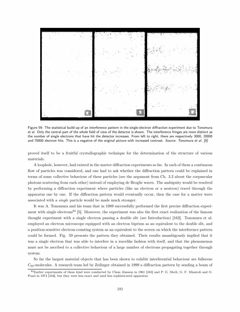
Figure 59: The statistical build-up of an interference pattern in the single-electron diffraction experiment due to Tonomuraet al. Only the central part of the whole field of view of the detector is shown. The interference fringes are more distinct asthe number of single electrons that have hit the detector increases. From left to right, there are respectively 3000, 20000and 70000 electron hits. This is a negative of the original picture with increased contrast. Source: Tonomura et al. [5]

proved itself to be a fruitful crystallographic technique for the determination of the structure of various

materials.

A loophole, however, had existed in the matter diffraction experiments so far. In each of them a continuous

flow of particles was considered, and one had to ask whether the diffraction pattern could be explained in

terms of some collective behaviour of these particles (see the argument from Ch. 3.2 about the corpuscular

photons scattering from each other) instead of employing de Broglie waves. The ambiguity would be resolved

by performing a diffraction experiment where particles (like an electron or a neutron) travel through the

apparatus one by one. If the diffraction pattern would eventually occur, then the case for a matter wave

associated with a single particle would be made much stronger.

It was A. Tonomura and his team that in 1989 successfully performed the first precise diffraction experi-

ment with single electrons82 [5]. Moreover, the experiment was also the first exact realization of the famous

thought experiment with a single electron passing a double slit (see Introduction) [162]. Tonomura et al.

employed an electron microscope equipped with an electron biprism as an equivalent to the double slit, and

a position-sensitive electron-counting system as an equivalent to the screen on which the interference pattern

could be formed. Fig. 59 presents the pattern they obtained. Their results unambigously implied that it

was a single electron that was able to interfere in a wavelike fashion with itself, and that the phenomenon

must not be ascribed to a collective behaviour of a large number of electrons propagating together through

system.

So far the largest material objects that has been shown to exhibit interferential behaviour are fullerene

C60-molecules. A research team led by Zeilinger obtained in 1999 a diffraction pattern by sending a beam of

82Earlier experiments of these kind were conducted by Claus Jönsson in 1961 [163] and P. G. Merli, G. F. Missiroli and G.Pozzi in 1974 [164], but they were less exact and used less sophisticated apparatus.

181

C60-molecules through a diffraction grating consisting of nominally 50 nm wide slits with a 100 nm period [44].

The velocity distribution of the molecules was measured and fitted; the most probable velocity corresponded

to a de Broglie wavelength of 2.5 pm which is approximately 400 smaller than the diameter of C60. It should

be stressed the total mass M of one molecule was used in calculating the de Broglie wavelength, i.e. it

was assumed that each interferring de Broglie wave corresponded to a single undivided particle of mass M .

Furthermore, the observations supported the view that each C60-molecule interferes with itself alone, even

though they did not propagate singly through the apparatus.

Many different experiments confirmed the validity of de Broglie’s relation between momentum and wave-

length of material objects. Although the relation does not make any explicit distinction between the macro-

scopic and the microscopic level, it has been verified only in the case of the latter. It remains to be seen

if analogous results will be obtained for still larger and more complicated molecules. If not, it will be very

interesting to see if it is the size, mass or rather the structure of the physical object under examination that

decides when the diffractive behaviour ceases to occur. It is also conceivable that the diffractive behaviour

of matter will persist, but that the simple de Broglie relation, Eq. (205), will have to be replaced by some

other formula which maybe will give us a better physical insight into the nature of the phenomenon.

Aside from looking for the upper spatial bound, there is another crucial question that could be answered

empirically. Imagine that an experiment similar to that of Zeilinger et al. is performed, but with slits in

the diffraction grating being considerably smaller than the size of the material object we wish to diffract.

Will the diffractive pattern still be obtained? If no, it would imply that there is something intrinsically solid

about the matter (in addition to the de Broglie waves) that does not allow a material object to propagate

through a slit which is smaller than the object itself (the size of the object being determined with help of

some different means). The persistence of the diffractive pattern, however, would suggest that – at least at

the microscopic level and under particular circumstances – the structure of matter is completely undulatory.

182

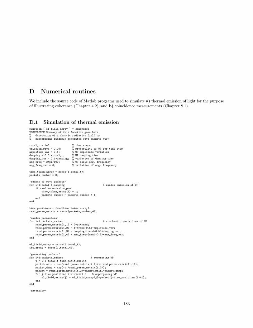
D Numerical routines

We include the source code of Matlab programs used to simulate a) thermal emission of light for the purposeof illustrating coherence (Chapter 4.2); and b) coincidence measurements (Chapter 8.1).

D.1 Simulation of thermal emissionfunction [ el_field_array ] = coherence%COHERENCE Summary of this function goes here% Generation of a chaotic radiative field by% superposing randomly generated wave packets (WP)

total_t = 1e5; % time stepsemission_prob = 0.05; % probability of WP per time stepamplitude_var = 0.1; % WP amplitude variationdamping = 0.01*total_t; % WP damping timedamping_var = 0.1*damping; % variation of damping timeang_freq = 2*pi/100; % WP basic ang. frequencyang_freq_var = 0; % variation of ang. frequency

time_token_array = zeros(1,total_t);packets_number = 0;

’number of wave packets’for i=1:total_t-damping % random emission of WP

if rand <= emission_probtime_token_array(i) = 1;packets_number = packets_number + 1;

endend

time_positions = find(time_token_array);rand_param_matrix = zeros(packets_number,4);

’random parameters’for i=1:packets_number % stochastic variations of WP

rand_param_matrix(i,1) = 2*pi*rand;rand_param_matrix(i,2) = 1+(rand-0.5)*amplitude_var;rand_param_matrix(i,3) = damping+(rand-0.5)*damping_var;rand_param_matrix(i,4) = ang_freq+(rand-0.5)*ang_freq_var;

end

el_field_array = zeros(1,total_t);int_array = zeros(1,total_t);

’generating packets’for i=1:packets_number % generating WP

t = 0:1:total_t-time_positions(i);packet_main = cos(rand_param_matrix(i,4)*t+rand_param_matrix(i,1));packet_damp = exp(-t./rand_param_matrix(i,3));packet = rand_param_matrix(i,2)*packet_main.*packet_damp;for j=time_positions(i):1:total_t % superposing WP

el_field_array(j) = el_field_array(j)+packet(j-time_positions(i)+1);end

end

’intensity’

183

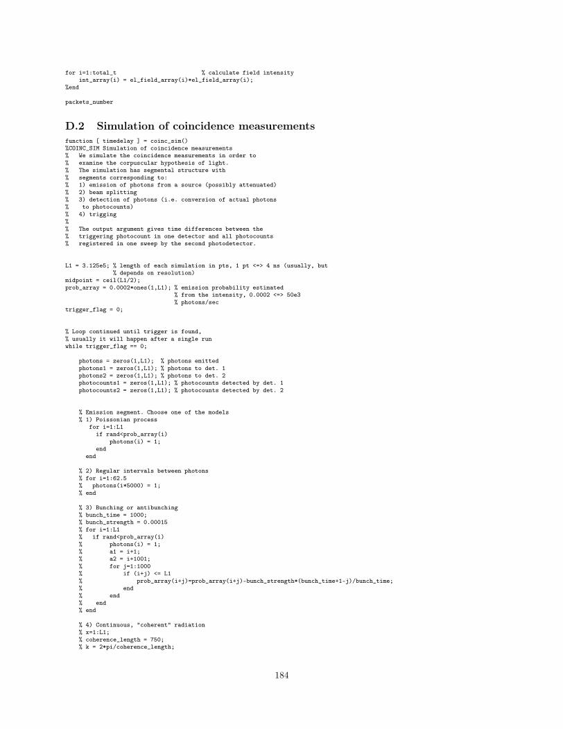
for i=1:total_t % calculate field intensityint_array(i) = el_field_array(i)*el_field_array(i);

%end

packets_number

D.2 Simulation of coincidence measurementsfunction [ timedelay ] = coinc_sim()%COINC_SIM Simulation of coincidence measurements% We simulate the coincidence measurements in order to% examine the corpuscular hypothesis of light.% The simulation has segmental structure with% segments corresponding to:% 1) emission of photons from a source (possibly attenuated)% 2) beam splitting% 3) detection of photons (i.e. conversion of actual photons% to photocounts)% 4) trigging%% The output argument gives time differences between the% triggering photocount in one detector and all photocounts% registered in one sweep by the second photodetector.

L1 = 3.125e5; % length of each simulation in pts, 1 pt <=> 4 ns (usually, but% depends on resolution)

midpoint = ceil(L1/2);prob_array = 0.0002*ones(1,L1); % emission probability estimated

% from the intensity, 0.0002 <=> 50e3% photons/sec

trigger_flag = 0;

% Loop continued until trigger is found,% usually it will happen after a single runwhile trigger_flag == 0;

photons = zeros(1,L1); % photons emittedphotons1 = zeros(1,L1); % photons to det. 1photons2 = zeros(1,L1); % photons to det. 2photocounts1 = zeros(1,L1); % photocounts detected by det. 1photocounts2 = zeros(1,L1); % photocounts detected by det. 2

% Emission segment. Choose one of the models% 1) Poissonian process

for i=1:L1if rand<prob_array(i)

photons(i) = 1;end

end

% 2) Regular intervals between photons% for i=1:62.5% photons(i*5000) = 1;% end

% 3) Bunching or antibunching% bunch_time = 1000;% bunch_strength = 0.00015% for i=1:L1% if rand<prob_array(i)% photons(i) = 1;% a1 = i+1;% a2 = i+1001;% for j=1:1000% if (i+j) <= L1% prob_array(i+j)=prob_array(i+j)-bunch_strength*(bunch_time+1-j)/bunch_time;% end% end% end% end

% 4) Continuous, "coherent" radiation% x=1:L1;% coherence_length = 750;% k = 2*pi/coherence_length;

184

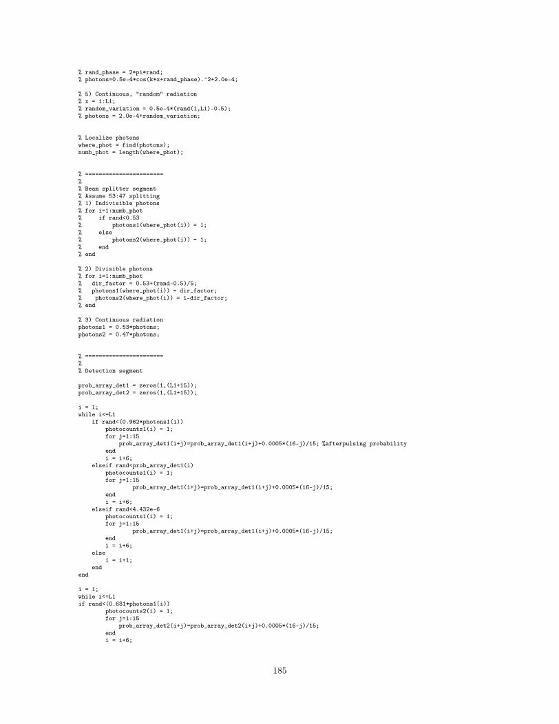
% rand_phase = 2*pi*rand;% photons=0.5e-4*cos(k*x+rand_phase).^2+2.0e-4;

% 5) Continuous, "random" radiation% x = 1:L1;% random_variation = 0.5e-4*(rand(1,L1)-0.5);% photons = 2.0e-4+random_variation;

% Localize photonswhere_phot = find(photons);numb_phot = length(where_phot);

% =======================%% Beam splitter segment% Assume 53:47 splitting% 1) Indivisible photons% for i=1:numb_phot% if rand<0.53% photons1(where_phot(i)) = 1;% else% photons2(where_phot(i)) = 1;% end% end

% 2) Divisible photons% for i=1:numb_phot% dir_factor = 0.53+(rand-0.5)/5;% photons1(where_phot(i)) = dir_factor;% photons2(where_phot(i)) = 1-dir_factor;% end

% 3) Continuous radiationphotons1 = 0.53*photons;photons2 = 0.47*photons;

% =======================%% Detection segment

prob_array_det1 = zeros(1,(L1+15));prob_array_det2 = zeros(1,(L1+15));

i = 1;while i<=L1

if rand<(0.962*photons1(i))photocounts1(i) = 1;for j=1:15

prob_array_det1(i+j)=prob_array_det1(i+j)+0.0005*(16-j)/15; %afterpulsing probabilityendi = i+6;

elseif rand<prob_array_det1(i)photocounts1(i) = 1;for j=1:15

prob_array_det1(i+j)=prob_array_det1(i+j)+0.0005*(16-j)/15;endi = i+6;

elseif rand<4.432e-6photocounts1(i) = 1;for j=1:15

prob_array_det1(i+j)=prob_array_det1(i+j)+0.0005*(16-j)/15;endi = i+6;

elsei = i+1;

endend

i = 1;while i<=L1if rand<(0.681*photons1(i))

photocounts2(i) = 1;for j=1:15

prob_array_det2(i+j)=prob_array_det2(i+j)+0.0005*(16-j)/15;endi = i+6;

185

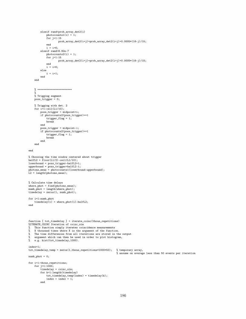
elseif rand<prob_array_det2(i)photocounts1(i) = 1;for j=1:15

prob_array_det2(i+j)=prob_array_det2(i+j)+0.0005*(16-j)/15;endi = i+6;

elseif rand<8.92e-7photocounts2(i) = 1;for j=1:15

prob_array_det2(i+j)=prob_array_det2(i+j)+0.0005*(16-j)/15;endi = i+6;

elsei = i+1;

endend

% =======================%% Trigging segmentposs_trigger = 0;

% Trigging with det. 2for i=1:ceil(L1/10);

poss_trigger = midpoint+i;if photocounts2(poss_trigger)==1

trigger_flag = 1;break

endposs_trigger = midpoint-i;if photocounts2(poss_trigger)==1

trigger_flag = 1;break

endend

end

% Choosing the time window centered about triggerhalfL2 = floor(L1/2)-ceil(L1/10);lowerbound = poss_trigger-halfL2+1;upperbound = poss_trigger+halfL2-1;photons_meas = photocounts1(lowerbound:upperbound);L2 = length(photons_meas);

% Calculate time delayswhere_phot = find(photons_meas);numb_phot = length(where_phot);timedelay = zeros(1, numb_phot);

for i=1:numb_phottimedelay(i) = where_phot(i)-halfL2;

end

function [ tot_timedelay ] = iterate_coinc(thous_repetitions)%ITERATE_COINC Iteration of coinc_sim% This function simply iterates coincidence measurements% X thousand times where X is the argument of the function.% The time differences from all iterations are stored in the output% argument which can then be used in order to plot histogram,% e.g. hist(tot_timedelay,1000).

index=1;tot_timedelay_temp = zeros(1,thous_repetitions*1000*50); % temporary array,

% assume on average less than 50 events per iterationnumb_phot = 0;

for i=1:thous_repetitions;for j=1:1000;

timedelay = coinc_sim;for k=1:length(timedelay)

tot_timedelay_temp(index) = timedelay(k);index = index + 1;

end

186

endi

end

tot_timedelay = tot_timedelay_temp(1:index-1);

187

188

References

[1] Roger Penrose, The Large, the Small and the Human Mind, Cambirdge University Press, 2000

[2] The Cambridge Dictionary of Philosophy, edited by Robert Audi, Cambridge University Press, SecondEdition, 1999

[3] Dictionary of Physics, edited by H.J. Gray and Alan Isaacs, Longman, 1990

[4] Richard P. Feynman, Robert B. Leighton, Matthew Sands, The Feynman Lectures on Physics, SecondEdition, vol. 3, Addison Wesley, 2005

[5] A. Tonomura, J. Endo, T. Matsuda, T. Kawasaki, H. Ezawa, Demonstration of single-electron buildupof an interference pattern, American Journal of Physics 57 (1989), pp. 117-120

[6] Martio Bertolotti, The History of the Laser, Taylor & Francis, 2004

[7] http://india_resource.tripod.com/physics.htm, retrieved on 9.09.2008

[8] Euclides, Optics, translated to English by Harry E. Burton, Journal of the Optical Society of America35 (1945), pp. 357-372

[9] Arne Næss, Filosofiens historie, Universitetsforlaget, 2001 (in Norwegian)

[10] http://muslimmedianetwork.com/mmn/?p=1886, retrieved on 9.09.2008

[11] George Sarton, Introduction to the history of science, Baltimore, 1927

[12] René Descartes, Optics (La dioptrique), from The Philosophical Writings of Descartes, translated byJohn Cottingham, Robert Stoothoff and Dugald Murdoch, Cambridge University Press, 1985

[13] René Descartes, Principles of Philosophy (Principia philosophiae), from The Philosophical Writingsof Descartes, translated by John Cottingham, Robert Stoothoff and Dugald Murdoch, CambridgeUniversity Press, 1985

[14] Andrzej Kajetan Wróblewski, Historia fizyki, Wydawnictwo Naukowe PWN, 2007 (in Polish)

[15] Edmé Mariotte, De la nature des couleurs, as quoted by [14]

[16] Christiaan Huygens, Treatise on light, translated by Silvanus P. Thompson, University of Chicago Press,www.gutenberg.org, retrieved on 9.09.2008

[17] Isaac Newton, The history of the Royal Society of London, vol. 3, p. 249, edited by T. Birch

[18] Isaac Newton, Answer to some Considerations upon his Doctrine of Light and Colors, PhilosophicalTransactions 88, pp. 5084-5103

[19] The history of the Royal Society of London, vol. 3, pp. 247-305, edited by T. Birch

[20] Isaac Newton, Opticks, Dover Publications, 1979

[21] I. Bernard Cohen, Preface to [20]

[22] Thomas Young, Bakerian Lecture on the Theory of Light and Colour, from Abstracts of the PapersPrinted in the Philosophical Transactions of the Royal Society of London, vol. 1, (1800 - 1814), pp.63-67

[23] Thomas Young, The Bakerian Lecture: Experiments and Calculations Relative to Physical Optics,Philosophical Transactions 94, pp. 1-16

189

[24] J. J. O’Connor, E. F. Robertson, Augustin Jean Fresnel, http://www-history.mcs.st-andrews.ac.uk/Biographies/Fresnel.html, retrieved on 30.09.2008

[25] James Clerk Maxwell, A Treatise on Electricity and Magnetism, Clarendon Press, Oxford, 1873, vol.2, p. 383

[26] http://scienceworld.wolfram.com/biography/Michelson.html, retrieved on 9.09.2008

[27] Otto Lummer, Ernst Pringsheim, Die Vertheilung der Energie im Spectrum des Körpers, Verhandlungender Deutschen Physikalischen Gesellschaft 1, pp. 23-41 (1899)

[28] Helge Kragh, Max Planck: the reluctant revolutionary, Physics World, December 2000

[29] Helge Kragh, Quantum Generations: A History of Physics in the Twentieth Century, Princeton Uni-versity Press, 1999

[30] Britannica Online Encyclopedia, www.britannica.com, photoelectric effect, retrieved on 9.09.2008

[31] Albert Einstein, Über einen die Erzeugung und Verwandlung des Lichtes betreffenden heuristis-chen Gesichtspunkt, Annalen der Physik 322, pp. 132-148 (1905); as translated by D. Ter Haar,http://lorentz.phl.jhu.edu/AnnusMirabilis/AeReserveArticles/eins_lq.pdf, retrieved on 25.11.2008

[32] Owen W. Richardson, The theory of photoelectric action, Philosophical Magazine 24, pp. 570-574 (1912)

[33] Arthur H. Compton, A Quantum Theory of the Scattering of X-Rays by Light Elements, Physical

Review 21, pp. 483-502 (1923)

[34] Niels Bohr, Hendrik Kramers, John Slater, The quantum theory of radiation, Philosophical Magazine47, 785-802 (1924)

[35] Jagdish Mehra, Helmut Rechenberg, The historical development of quantum theory, Springer-Verlag,1982, Vol. 1, Part 2, pp. 532-554

[36] Louis de Broglie, Recherches sur la théorie des quanta, doctoral thesis, Paris, 1924; as translated byA. F. Kracklauer, http://www.ensmp.fr/aflb/LDB-oeuvres/De_Broglie_Kracklauer.pdf, retrieved on15.09.2008

[37] Clinton Davisson, Lester Germer, Reflection of electrons by a crystal of nickel, Nature 119, pp. 558-560(1927)

[38] Immanuel Estermann, Otto Stern, Beugung von Molekularstrahlen, Zeitschrift für Physik 61, pp. 95-125(1930)

[39] David Bohm, B. J. Hiley, The Undivided Universe: An ontological interpretation of quantum theory,Routledge, 1995

[40] Edwin Jaynes, Leonard Mandel, Survey of the present status of neoclassical radiation theory, in: Pro-ceedings of the Third Rochester Conference on Coherence and Quantum Optics, Plenum Press, 1973,pp. 35-81

[41] R. Hanbury Brown, R. Q. Twiss, A Test of a New Type of Stellar Interferometer on Sirius, Nature177, p. 27 (1956)

[42] P. W. Milonni, Wave-Particle Duality of Light: A Current Perspective, in: The Wave-Particle Dualism,pp. 27-67, Springer, 1983

[43] Roy J. Glauber, The Quantum Theory of Optical Coherence, Physical Review 130, pp. 2529-2539 (1963)

190

[44] M. Arndt, O. Nairz, J. Vos-Andreae, C. Keller, G. van der Zouw, A. Zeilinger, Wave-particle duality ofC60 molecules, Nature 401 , pp. 680-682 (1999)

[45] Shahriar Afshar, Sharp complementary wave and particle behaviours in the same “welcher Weg” exper-iment, Proceedings of SPIE 5866, pp. 229-244 (2005)

[46] Shahriar Afshar, Eduardo Flores, Keith McDonald, Ernst Knoesel, Paradox in Wave-Particle Duality,Foundation of Physics 37, pp. 295-305 (2007)

[47] Nannapaneni Narayana Rao, Elements of Engineering Electromagnetics, 6th Edition, Prentice Hall,2004

[48] Bahaa E. A. Saleh, Malvin Carl Teich, Fundamentals of Photonics, Second Edition, Wiley, 2007

[49] John D. Jackson, Classical Electrodynamics, Third Edition, Wiley, 1998

[50] http://eclectricz.blogspot.com/2007/05/let-there-be-light-as-hertz-proved.html, retrieved on16.09.2008

[51] Ramamurti Shankar, Principles of Quantum Mechanics, Second Edition, Springer, 1994

[52] Rodney Loudon, The Quantum Theory of Light, Third Edition, Oxford University Press, 2000

[53] Julian Schwinger, Lester L. Deraad, Kimball A. Milton, Wu-yang Tsai, Joyce Norton, Classical Elec-trodynamics, Westview Press, 1998

[54] E. A. Power, Introductory Quantum Electrodynamics, Longmans, 1964

[55] Leonard Mandel, Emil Wolf, Optical Coherence and Quantum Optics, Cambridge University Press,1995

[56] D. F. Walls, G. J. Milburn, Quantum Optics, Springer-Verlag, 1994

[57] Mark Fox, Quantum Optics: An Introduction, Oxford University Press, 2006

[58] David Chandler, Introduction to Modern Statistical Mechanics, Oxford University Press, 1987

[59] Max Planck, Über das Gesetz der Energieverteilung im Normalspectrum, Annalen der Physik 309, pp.553-563 (1901); translation retrieved from http://bourabai.narod.ru/articles/planck/planck1901.pdf on21.01.2009

[60] H. Rubens, F. Kurlbaum, Proceedings of the Imperial Academy of Science, Berlin, 25.10.1900, p. 929

[61] H. Beckmann, Inaugural dissertation, Tubingen 1898. See also: H. Rubens, Weid. Ann. 69, p. 582(1899)

[62] Martin White, Anisotropies in the CMB, http://arxiv.org/abs/astro-ph/9903232v1, retrieved on21.01.2009

[63] Dictionary of Pure and Applied Physics, edited by Dipak Basu, CRC, 2000

[64] George S. Monk, Light: Principles and Experiments, First Edition, McGraw-Hill Book Company, 1937

[65] A Dictionary of Physics, edited by John Daintith, Oxford University Press, 2005

[66] Britannica Online Encyclopedia, www.britannica.com, optical interferometer, retrieved on

19.11.2008

[67] R. W. Ditchburn, Light, Academic Press, 1976

191

[68] A. A. Michelson, Inteference Phenomena in a New Form of Refractometer, Philosophical Magazine 13,

pp. 236-242 (1882)

[69] Richard Feynman, QED: The Strange Theory of Light and Matter, Princeton University Press, 2006

[70] F. Selleri, “Gespensterfelder”, in: The Wave-Particle Dualism, pp. 101-128, Springer, 1983

[71] E. Panarella, Nonlinear behaviour of light at very low intensities: The “photon clump” model, in: Quan-tum Uncertainties, Plenum Press, 1986, pp. 105-167

[72] L. János, Zs. Náray, Investigation into interference phenomena at extremely low light intensities bymeans of a large Michelson interferometer, Il Nuovo Cimento 9 (Supplement 2), pp. 588-598 (1958)

[73] John F. Clauser, Experimental distinction between the quantum and classical field-theoretic predictionsfor the photoelectric effect, Physical Review D 9, pp. 853-860 (1974)

[74] Philipp Lenard, Über die lichtelektrische Wirkung, Annalen der Physik 313, pp. 149-198 (1902)

[75] O. W. Richardson, K. T. Compton, The Photoelectric Effect, Philosophical Magazine 24, pp. 575-594(1912)

[76] P. W. Milonni, Answer to Question #45, Questions and Answers, American Journal of Physics 64, pp.11-12 (1997)

[77] O. W. Richardson, Some Applications of the Electron Theory of Matter, Philosophical Magazine 23,

pp. 594-627 (1912)

[78] Charles Erwin Tyler, The Element of Time in the Photoelectric Effect, 1969, Ph.D. thesis, Washington

University

[79] W. Davis, L. Mandel, Time Delay Statistics of Photoelectric Emissions: An Experimental Test of Clas-

sical Radiation Theory, in: Proceedings of the Third Rochester Conference on Coherence and Quantum

Optics, Plenum Press, 1973, pp. 113-119

[80] Leonard Mandel, The Case for and against Semiclassical Radiation Theory, Progress in Optics 13, pp.27-68, North-Holland (1976)

[81] Frank C. Jones, Calculated Spectrum of Inverse-Compton-Scattered Photons, Physical Review 167, pp.1159-1169 (1968)

[82] Peter Debye, Zerstreuung von Rontgenstrahlen und Quantentheorie, Physikalische Zeitschrift 24 8, pp.161-166 (1923)

[83] R. E. Bell, R. L. Graham, Measurement of a Second Half-Life in Yb170, Physical Review 78, pp. 490-491(1950)

[84] Chandrasekhara Venkata Raman, A Classical Derivation of the Compton Effect, Indian Journal ofPhysics 3, pp. 357-369 (1928)

[85] Richard Kidd, James Ardini, Anatol Anton, Compton effect as a double Doppler shift, American Journalof Physics 53, pp. 641-644 (1985)

[86] Walter Roy Mellen, Compton effect from a center-of-momentum system, American Journal of Physics49, pp. 505-506 (1981)

192

[87] Malcom J. Cooper, Compton scattering and electron momentum determination, Reports on Progressin Physics 48, pp. 415-481 (1985)

[88] J. N. Dodd, The scattering of electromagnetic radiation by a free electron, Journal of Physics B 8, pp.157-164 (1975)

[89] Philippe Grangier, Gerard Roger, Alain Aspect, Experimental Evidence for a Photon AnticorrelationEffect on a Beam Splitter: A New Light on Single-Photon Interference, Europhysics Letters 1, pp.173-179 (1986)

[90] Alain Aspect, Philippe Grangier, Gerard Roger, Experimental Tests of Realistic Local Theories viaBell’s Theorem, Physical Review Letter 47, pp. 460-463 (1981)

[91] J. Dugundji, Envelopes and pre-envelopes of real waveforms, IRE Transactions on Information Theory,

1958

[92] Marian O. Scully, Murray Sargent III, The Concept of the Photon, Physics Today, March 1972

[93] Michael G. Raymer, Observations of the modern photon, Letter to the Editor, American Journal ofPhysics 58, p. 11 (1990)

[94] Leonard Mandel, Emil Wolf, The Measures of Bandwidth and Coherence Time in Optics, Proceedings

of the Physical Society 80, pp. 894-897 (1962)

[95] Emil Wolf, Reciprocity Inequalities, Coherence Time and Bandwidth in Signal Analysis and Optics,

Proceedings of the Physical Society 71, pp. 257-269 (1958)

[96] Leonard Mandel, Fluctuations of Photon Beams: The Distribution of the Photo-Electrons, Proceedings

of the Physical Society 74, pp. 233-243 (1959)

[97] R. Hanbury Brown, R. Q. Twiss, Interferometry of the Intensity Fluctuations in Light. I. Basic Theory:

The Correlation between Photons in Coherent Beams of Radiation, Proceedings of the Royal Society A

242, pp. 300-324 (1957)

[98] R. Hanbury Brown, R. Q. Twiss, Interferometry of the Intensity Fluctuations in Light II. An Experi-

mental Test of the Theory for Partially Coherent Light, Proceedings of the Royal Society A 243, pp.

291-319 (1958)

[99] Rodney Loudon, Non-classical effects in the statistical properties of light, Reports on Progress in Physics43, pp. 913-949 (1980)

[100] Peter W. Milonni, Joseph H. Eberly, Lasers, First Edition, Wiley-Interscience, 1988

[101] A. E. Siegman, Lasers, University Science, 1986

[102] K. F. Riley, M. P. Hobson, S. J. Bence, Mathematical Methods for Physics and Engineering, Second

Edition, Cambridge University Press

[103] P. L. Kelley, W. H. Kleiner, Theory of electromagnetic field measurement and photoelectron counting,

Physical Review 136, pp. A316-A334 (1964)

193

[104] A. C. Funk, M. Beck, Sub-Poissonian photocurrent statistics: Theory and undergraduate experiment,

American Journal of Physics 65, pp. 492-500 (1997)

[105] X. T. Zou, L. Mandel, Photon-antibunching and sub-Poissonian photon statistics, Physical Review A41, pp. 475-476 (1990)

[106] R. Short, L. Mandel, Observation of Sub-Poissonian photon statistics, Physical Review Letters 51, pp.384-387 (1983)

[107] M. C. Teich, B. E. A. Saleh, Observation of sub-Poisson Franck-Hertz light at 253.7 nm, Journal of theOptical Society of America B 2, pp. 275-282 (1985)

[108] P. R. Tapster, J. G. Rarity, J. S. Satchell, Use of parametric down-conversion to generate sub-Poissonianlight, Physical Review A 37, pp. 2963-2967 (1988)

[109] H. J. Kimble, M. Dagenais, L. Mandel, Photon Antibunching in Resonance Fluorescence, PhysicalReview Letters 39, pp. 691-695 (1977)

[110] Ch. Kurtsiefer, S. Mayer, P. Zarda, H. Weinfurter, Stable Solid-State Source of Single Photons, PhysicalReview Letters 85, pp. 290-293 (2000)

[111] Ch. Santori, M. Pelton, G. Solomon, Y. Dale, Y. Yamamoto, Triggered Single Photons from a QuantumDot, Physical Review Letters 86, pp. 1502-1505 (2001)

[112] Hans-A. Bachor, Timothy C. Ralph, A Guide to Experiments in Quantum Optics, Wiley, Second

Edition, 2004

[113] A. Gerrard, J. M. Burch, Introduction to Matrix Methods in Optics, Dover Publications, 1994

[114] http://optoelectronics.perkinelmer.com/catalog/Product.aspx?ProductID=SPCM-AQRH-16, re-

trieved on 22.02.2009

[115] http://optoelectronics.perkinelmer.com/content/Datasheets/DTS_SPCMAQRH.pdf, retrieved on

22.02.2009

[116] Newport, http://search.newport.com/?sku=05BC16PC.4, retrieved on 6.04.2009

[117] Thorlabs, http://www.thorlabs.com/thorProduct.cfm?partNumber=WPH05M-633, retrieved on6.04.2009

[118] Thorlabs, http://www.thorlabs.com/NewGroupPage9.cfm?ObjectGroup_ID=266, retrieved on6.04.2009

[119] http://www.newport.com/Laser-Line-Non-Polarizing-Cube-Beamsplitters/141121/1033/catalog.aspx,

retrieved on 20.02.2009

[120] Thorlabs, http://www.thorlabs.com/Thorcat/12100/12109-S01.PDF, retrieved on 12.12.2008

[121] Thorlabs, http://www.thorlabs.com/thorProduct.cfm?partNumber=ES120, retrieved on 6.04.2009

[122] Thorlabs, http://www.thorlabs.com/catalogPages/951.pdf, retrieved on 6.04.2009

[123] LeCroy, http://www.lecroy.com/tm/products/scopes/specs.asp?mseries=25, retrieved on 6.04.2009

194

[124] Daniel M. Greenberger, Allaine Yasin, Simultaneous Wave and Particle Knowledge in a Neutron Inter-ferometer, Physics Letters A 128, pp. 391-394 (1988)

[125] Gregg Jaeger, Abner Shimony, Lev Vaidman, Two interferometric complementarities, Physical ReviewA 51, pp. 54-67 (1995)

[126] Berthold-Georg Englert, Fringe Visibility and Which-Way Information: An Inequality, Physical ReviewLetters 77, pp. 2154-2157 (1996)

[127] Niels Bohr, The Quantum Postulate and the Recent Development of Atomic Theory, Nature 121, pp.580-590 (1928)

[128] R. E. Kastner, Why the Afshar Experiment Does Not Refute Complementarity,http://arxiv.org/abs/quant-ph/0502021, retrieved on 24.04.2009

[129] Eduardo Flores, Ernst Knoesel, Why Kastner analysis does not apply to a modified Afshar experiment,http://arxiv.org/abs/quant-ph/0702210, retrieved on 24.04.2009

[130] Aurelien Drezet, Complementarity and Afshar’s experiment, http://arxiv.org/abs/quant-ph/0508091,retrieved on 24.04.2009

[131] Tabish Qureshi, Complementarity and the Afshar Experiment, http://arxiv.org/abs/quant-ph/0701109,retrieved on 24.04.2009

[132] Ole Steuernagel, Afshar’s Experiment Does Not Show a Violation of Complementarity, Foundations ofPhysics 37, pp. 1370-1385 (2007)

[133] Eduardo Flores, Reply to Comments of Steuernagel on the Afshar’s Experiment, Foundation of Physics38, pp. 778-781 (2008)

[134] Max Born, Emil Wolf, Principles of Optics, Second Edition, Pergamon Press, 1964

[135] J. P. Girardeau-Montaut, C. Girardeau-Montaut, Theory of ultrashort nonlinear multiphoton photo-electric emission from metals, Physical Review B 51, pp. 13560-13567 (1995)

[136] Stanford Encyclopedia of Philosophy, Copenhagen Interpretation of Quantum Mechanics,

http://plato.stanford.edu/entries/qm-copenhagen/, retrieved on 2.05.2009

[137] Franco Selleri, Quantum Paradoxes and Physical Reality, Kluwer Academic Publishers, 1990

[138] Dugald Murdoch, Niels Bohr’s Philosophy of Physics, Cambridge University Press, 1989

[139] Niels Bohr, The Quantum Postulate and the Recent Development of Atomic Theory, Nature 121, pp.

580-590 (1928)

[140] Asher Peres, Carl Popper and the Copenhagen Interpretation, Studies In History and Philosophy of

Science Part B: Studies In History and Philosophy of Modern Physics 33, pp. 23-34 (2002), preprint

available at http://arxiv.org/abs/quant-ph/9910078m, retrieved on 3.05.2009

[141] Encyclopaedic Dictionary of Physics, vol. 2, editor-in-chief: J. Thewlis, Pergamon Press, 1961

[142] Leon Rosenfeld, The Wave-Particle Dilemma, in: The Physicist’s Conception of Nature, edited by

Jagdish Mehra, Springer, 2007, available on http://books.google.no, retrieved on 3.05.2009

195

[143] William K. Wootters, Wojciech H. Zurek, Complementarity in the double-slit experiment: Quantum

nonseparability and a quantitative statement of Bohr’s principle, Physical Review D19, pp. 473-484

(1979)

[144] D. Bohm, A Suggested Interpretation of the Quantum Theory in terms of “Hidden” Variables I, Physical

Review 85, pp. 166-179 (1952)

[145] D. Bohm, A Suggested Interpretation of the Quantum Theory in Terms of "Hidden” Variables II,Physical Review 85, pp. 180-193 (1952)

[146] David Bohm, Reply to a Criticism of a Causal Re-Interpretation of the Quantum Theory, Physical

Review 57, pp. 389-390 (1952)

[147] Otto Halpern, A Proposed Re-Interpretation of Quantum Mechanics, Physical Review 57, p. 389 (1952)

[148] C. Philippidis, C. Dewdney, B. J. Hiley, Quantum interference and the quantum potential, Il Nuovo

Cimento B52, pp. 15-28 (1979)

[149] C. Dewdney, B. J. Hiley, A Quantum Potential Description of One-Dimensional Time-Dependent Scat-

tering From Square Barriers and Square Wells, Foundation of Physics 12, pp. 27-48 (1982)

[150] Will Keepin, Lifework of David Bohm – River of Truth, http://www.vision.net.au/~apaterson/science/david_bohm.htm, retrieved on 7.05.2009

[151] N. David Mermin, What’s Wrong with this Pillow?, Physics Today, April 1989, p. 9

[152] Chris J. Isham, Lectures on Quantum Theory: Mathematical and Structural Foundations, World Scien-

tific Publishing Company, 1995

[153] P. A. M. Dirac, Lectures on Quantum Mechanics, Dover Publications, 2001

[154] David J. Griffiths, Introduction to Quantum Mechanics, Second Edition, Prentice Hall, 2005

[155] F. Riesz, B. Sz.-Nagy, Functional Analysis, Section 21, Unger, 1955

[156] Jon Magne Leinaas, Non-Relativistic Quantum Mechanics, lecture notes, University ofOslo, 2008, http://www.uio.no/studier/emner/matnat/fys/FYS4110/h08/undervisningsmateriale/LectureNotes2008.pdf, retrieved on 10.10.2008

[157] William H. Louisell, Quantum Statistical Properties of Radiation, Chapter 3, Wiley, 1990

[158] Kevin E. Cahill, Coherent-State Representations for the Photon Density Operator, Physical Review138, p. B1566 (1965)

[159] Clinton Davisson, Lester Germer, Diffraction of Electrons by a Crystal of Nickel, Physical Review 30,pp. 705-740 (1927)

[160] George P. Thomson, Andrew Reid, Diffraction of Cathode Rays by a Thin Film, Nature 119, p. 890(1927)

[161] Ernest O. Wollan, C. G. Shull, The Diffraction of Neutrons by Crystalline Powders, Physical Review73, pp. 830-841 (1948)

196

[162] Peter Rodgers, The double-slit experiment, Physics World, http://physicsworld.com/cws/article/print/9745, retrieved on 4.12.2008

[163] Claus Jönsson, Electron Diffraction at Multiple Slits, American Journal of Physics 42, pp. 4-11 (1974);translation of a paper which originally appeared in: Zeitschrift für Physik 161, p. 454 (1961)

[164] P. G. Merli, G. F. Missiroli, G. Pozzi, On the statistical aspect of electron interference phenomena,American Journal of Physics 44, pp. 306-307 (1976)

197