biomimetic control with a feedback coupled …biomimetic.pbworks.com/f/biomimetic control with a...
TRANSCRIPT
BIOMIMETIC CONTROL WITH A FEEDBACK COUPLED
NONLINEAR OSCILLATOR:
INSECT EXPERIMENTS, DESIGN TOOLS, AND HEXAPEDAL
ROBOT ADAPTATION RESULTS
a dissertation
submitted to the department of mechanical engineering
and the committee on graduate studies
of stanford university
in partial fulfillment of the requirements
for the degree of
doctor of philosophy
Sean Ashley Bailey
July 2004

c© Copyright by Sean Ashley Bailey 2004
All Rights Reserved
ii

I certify that I have read this dissertation and that, in my opinion,
it is fully adequate in scope and quality as a dissertation for the
degree of Doctor of Philosophy.
Mark R. Cutkosky(Principal Adviser)
I certify that I have read this dissertation and that, in my opinion,
it is fully adequate in scope and quality as a dissertation for the
degree of Doctor of Philosophy.
Gunter Niemeyer
I certify that I have read this dissertation and that, in my opinion,
it is fully adequate in scope and quality as a dissertation for the
degree of Doctor of Philosophy.
J. Christian Gerdes
I certify that I have read this dissertation and that, in my opinion,
it is fully adequate in scope and quality as a dissertation for the
degree of Doctor of Philosophy.
Robert J. Full(Department of Integrative BiologyUniversity of California, Berkeley)
Approved for the University Committee on Graduate Studies.
iii
Abstract
Robotics has drawn inspiration from nature for many years, but only recently has an understanding
of the musculoskeletal dynamics of animal running been successfully implemented in small, self-
stabilizing legged robots. One such example is the biomimetic hexapod Sprawlita, capable of running
at over 2 bodylengths per second and traversing hip-height obstacles, all without feedback control.
Motivated by the question of how these robots can take advantage of feedback information, this
thesis explores sensory-mediated cyclic dynamic tasks - in animals, legged robots, and dynamic
systems in general - toward understanding the mechanisms and functional roles of sensory feedback
and a general approach for designing adaptive controllers.
To explore sensory-mediated cyclic behaviors in animals, cockroaches running on an inertial
treadmill are subjected to sustained oscillatory perturbations and electromyograms are recorded to
determine a phase measure relative to the perturbation. Experimental results show the use of sensory
feedback, even at the highest speeds of locomotion. The cockroach motor pattern generators are
modeled using a feedback coupled nonlinear oscillator and a numerical simulation is used to generate
predicted results. The observed behavior is consistent with these predictions and a statistical test
is used to quantify the phase measure distributions.
Feedback coupled nonlinear oscillators as controllers for cyclic dynamic systems are then exam-
ined, focusing on designing for adaptation to changing environmental conditions. An existing visual
design method is expanded upon, creating an intuitive three dimensional representation of the plant
and the nonlinear oscillator controller as conditions change, visually predicting the coupled system
adaptive behavior. An analysis tool, the ω contour analysis, is developed and used to determine
the appropriate feedback characteristics. In addition, a new method for tuning the coupled system
behavior using intentional time delays is presented.
Finally, this thesis concludes by using the design tools developed to create an adaptive, feedback
coupled nonlinear oscillator controller for a numerical simulation of the robot Sprawlita. The ω
contour analysis helps determine the appropriate feedback for the behavior desired, and additional
design tools are developed for feedback coupled nonlinear oscillator systems with binary actuation
and feedback. With the biologically-inspired adaptive controller, the robot runs up slopes 33%
iv
faster than in the open-loop configuration. In the process of designing this controller, a more in-
depth understanding of the robot locomotion on slopes is developed. In addition, the coupled system
behavior is examined and the mechanism through which the feedback signal creates the behavior
observed is explained.
Overall, this thesis outlines a biologically-inspired approach for achieving adaptive behaviors.
While the particular design example here is a biologically-inspired running robot, the design and
analysis tools developed are general, and can be used to design a feedback coupled nonlinear oscillator
controller to produce arbitrary adaptive behaviors for any cyclic dynamic system.
v

Acknowledgments
First, I’d like to thank Mark Cutkosky, my thesis adviser. Mark, you’ve made this all possible.
Thanks for letting me explore all of my hairbrained ideas, the ones that did and the ones that didn’t
work out. You’ve always given me the freedom and support I needed to pursue my own interests,
and I appreciate that. I sincerely thank you for having made my Ph.D. the experience that it was.
I’d also like to thank the rest of my reading committee, Gunter Niemeyer, Chris Gerdes, and
Bob Full. Thanks to each one of you for taking the time to read and help out with my thesis. I’d
especially like to thank Bob Full for letting me work at his lab in Berkeley on a regular basis for the
last 3 years. Please, replace the chairs, though - they really hurt after a long day. Gunter, I enjoyed
being your TA for two fun classes - thanks for always being patient with my questions and taking
the time to talk with me about anything and everything.
Thuy, so much of this is because of you, and I am not just talking about all of your help with
the figures. To me, you’ve been a part of this thesis since day one - you always believed in me and
encouraged me to keep going when I was ready to give up. I thank you for your friendship, and your
love - it made these last six months bearable. I’ll help you look for your glasses and dig illegal holes
any day. I can’t wait for our next adventure.
Wes, at least now I understand what you were going through last year. I can’t even begin to
list the ways it was fun just having you around - Stanford became a different place for me when
you left. I’ll always miss our days of biking, snowboarding, frisbee, getting chased by drooling cows,
shooting pool, teaching Margy to drive a stick-shift, “hanging out” at Will’s place (you know, near
the highway), bulls, horses, flamingos, and all the other great times we spent together.
Will, you can make everything with the car. Thanks for becoming such a good friend over the
last few years - it was really fun hanging out in Italy, and I always looked forward to Saturday Taco
Bell and your long-winded tales. Tell Pam I didn’t take her chair. Margy, I’m glad Wes and I walked
up and said “hi” so many years ago - you’ve been a close friend, you’ve been one of the people that
has really made this journey enjoyable for me. Jenny, I feel like I’ve finally gotten to know you
better after all these years - I hope it continues. Moto, I won’t hold you to our bet (though I can’t
speak for Wes) - I hope we get to go surfing again soon. Have fun and enjoy the rest of your time
here. Jason and Thyda - I miss you guys. I will make it up there someday...
vi
Jonathan Clark, we started together and now we’re ending together. I should say thanks for
the robot simulation (Chapter 6), but I’m really much more thankful for your patience and your
friendship. I wish you and your family the best, I hope we do cross paths again in the future.
I’d especially like to thank all the (other) people in the DML: Costa, Turner, Chris, Allison,
Jonathan Karpick, Li, Emily, Trey, Miguel, Dan, Niels, Jorge, Lewis, Sangbae, Roman, and everyone
else I can’t think of right now (hey, I’ve been getting no sleep!) - from movie and card nights to
camping trips and our now famous Halloween costumes, it’s been so much fun to be a part of this
lab. I feel like both the last one to go and the first one to leave. To all of you, my second family,
thanks for always making it such a great place to be.
I’d also like to thank the PolyPedal lab at UC Berkeley and the ARTS/CRIM lab in Pisa. Thanks
for taking me in and making me feel at home, especially Juliann, Anne, Dan, Noah, Pietro, l’altro
Pietro, and Luca.
Thanks to everyone else that supported me and helped out along the way: Chris Atkeson,
Farrokh Mistree, Gary McMurray, Noelle, Jeff, Judy, Matt Williamson, Rob Lingscheit, Andy Milne,
Lawrence, Rob Howe, Emma, Reza Shadmehr, and John Dorman, to name just a few.
Mom, Dad, Sharon - last, but not least. You’ve always been there for me and always been
supportive, so much so that I often take it all for granted. Thank you.
The Office of Naval Research supported this work under grant N00014-98-1-0669. I also received
funding from the National Science Foundation through a dissertation enhancement award (0138436)
and was supported by an NDSEG fellowship for my first three years at Stanford. I am deeply
grateful in each case.
vii

Contents
Abstract iv
Acknowledgments vi
1 Introduction 1
1.1 Motivation . . . . . . . . . . . . . . . . . . . . . . . . . . . . . . . . . . . . . . . . . 2
1.2 Approach . . . . . . . . . . . . . . . . . . . . . . . . . . . . . . . . . . . . . . . . . . 2
1.3 Contributions . . . . . . . . . . . . . . . . . . . . . . . . . . . . . . . . . . . . . . . . 3
1.4 Outline . . . . . . . . . . . . . . . . . . . . . . . . . . . . . . . . . . . . . . . . . . . 3
2 Previous work 5
2.1 History . . . . . . . . . . . . . . . . . . . . . . . . . . . . . . . . . . . . . . . . . . . 5
2.1.1 The first steps . . . . . . . . . . . . . . . . . . . . . . . . . . . . . . . . . . . 6
2.1.2 Dynamic legged robots . . . . . . . . . . . . . . . . . . . . . . . . . . . . . . . 6
2.1.3 Biomimetic robots . . . . . . . . . . . . . . . . . . . . . . . . . . . . . . . . . 7
2.1.4 Biomimetic control structure . . . . . . . . . . . . . . . . . . . . . . . . . . . 9
2.2 Closing the loop: feedback modification of motor patterns . . . . . . . . . . . . . . . 9
2.2.1 Task specific . . . . . . . . . . . . . . . . . . . . . . . . . . . . . . . . . . . . 9
2.2.2 Dynamics based . . . . . . . . . . . . . . . . . . . . . . . . . . . . . . . . . . 11
2.3 Nonlinear oscillators for locomotion control . . . . . . . . . . . . . . . . . . . . . . . 12
2.3.1 Inter-limb coordination for gait generation . . . . . . . . . . . . . . . . . . . . 12
2.3.2 Reflex gating . . . . . . . . . . . . . . . . . . . . . . . . . . . . . . . . . . . . 13
2.4 Feedback coupling a nonlinear oscillator . . . . . . . . . . . . . . . . . . . . . . . . . 13
2.4.1 Ring rules for stability . . . . . . . . . . . . . . . . . . . . . . . . . . . . . . . 15
2.4.2 Adaptation to uneven terrain . . . . . . . . . . . . . . . . . . . . . . . . . . . 16
2.5 Summary . . . . . . . . . . . . . . . . . . . . . . . . . . . . . . . . . . . . . . . . . . 16
3 Nonlinear oscillators 18
3.1 A short history . . . . . . . . . . . . . . . . . . . . . . . . . . . . . . . . . . . . . . . 19
viii
3.1.1 The van der Pol oscillator . . . . . . . . . . . . . . . . . . . . . . . . . . . . . 19
3.1.2 The Rayleigh oscillator . . . . . . . . . . . . . . . . . . . . . . . . . . . . . . 20
3.2 Nonlinear oscillator characteristics . . . . . . . . . . . . . . . . . . . . . . . . . . . . 20
3.2.1 Self-sustained limit cycle generation . . . . . . . . . . . . . . . . . . . . . . . 20
3.2.2 Selective entrainment . . . . . . . . . . . . . . . . . . . . . . . . . . . . . . . 23
3.3 Neurally-based nonlinear oscillators . . . . . . . . . . . . . . . . . . . . . . . . . . . . 27
3.3.1 The neuron . . . . . . . . . . . . . . . . . . . . . . . . . . . . . . . . . . . . . 27
3.3.2 The Hodgkin-Huxley neuron model . . . . . . . . . . . . . . . . . . . . . . . . 28
3.3.3 The Matsuoka oscillator . . . . . . . . . . . . . . . . . . . . . . . . . . . . . . 29
4 Biological inspiration 33
4.1 Previous work on pattern generators . . . . . . . . . . . . . . . . . . . . . . . . . . . 34
4.1.1 Central pattern generators . . . . . . . . . . . . . . . . . . . . . . . . . . . . . 34
4.1.2 Sensory modulation . . . . . . . . . . . . . . . . . . . . . . . . . . . . . . . . 35
4.1.3 Wendler’s experiments . . . . . . . . . . . . . . . . . . . . . . . . . . . . . . . 35
4.2 Cockroach experiments . . . . . . . . . . . . . . . . . . . . . . . . . . . . . . . . . . . 36
4.2.1 Locomotion model . . . . . . . . . . . . . . . . . . . . . . . . . . . . . . . . . 37
4.2.2 Experimental specifics . . . . . . . . . . . . . . . . . . . . . . . . . . . . . . . 37
4.2.3 Phase measure . . . . . . . . . . . . . . . . . . . . . . . . . . . . . . . . . . . 44
4.3 Simulated results . . . . . . . . . . . . . . . . . . . . . . . . . . . . . . . . . . . . . . 47
4.3.1 The simulation model . . . . . . . . . . . . . . . . . . . . . . . . . . . . . . . 47
4.3.2 Simulation boundary conditions . . . . . . . . . . . . . . . . . . . . . . . . . . 48
4.3.3 Directional statistics . . . . . . . . . . . . . . . . . . . . . . . . . . . . . . . . 51
4.4 Experimental results . . . . . . . . . . . . . . . . . . . . . . . . . . . . . . . . . . . . 55
4.4.1 Control trials . . . . . . . . . . . . . . . . . . . . . . . . . . . . . . . . . . . . 55
4.4.2 Perturbation trials . . . . . . . . . . . . . . . . . . . . . . . . . . . . . . . . . 57
5 Designing a feedback coupled nonlinear oscillator 61
5.1 General tools for design and analysis . . . . . . . . . . . . . . . . . . . . . . . . . . . 62
5.1.1 Linear systems . . . . . . . . . . . . . . . . . . . . . . . . . . . . . . . . . . . 62
5.1.2 Nonlinear systems . . . . . . . . . . . . . . . . . . . . . . . . . . . . . . . . . 63
5.2 Design with a feedback coupled nonlinear oscillator: a visual method . . . . . . . . . 66
5.2.1 System architecture . . . . . . . . . . . . . . . . . . . . . . . . . . . . . . . . 66
5.2.2 The graphical design method . . . . . . . . . . . . . . . . . . . . . . . . . . . 67
5.2.3 Shaping the plant and controller: Adjusting gains . . . . . . . . . . . . . . . 67
5.2.4 Shaping the plant: Rotations by negation, derivatives . . . . . . . . . . . . . 72
5.2.5 Shaping the controller: Adjusting the Matsuoka nonlinear oscillator parameters 73
5.2.6 Design considerations . . . . . . . . . . . . . . . . . . . . . . . . . . . . . . . 81
ix

5.3 Designing for changing dynamic conditions . . . . . . . . . . . . . . . . . . . . . . . 81
5.3.1 Example: A simplified model of running over changing slopes . . . . . . . . . 84
5.3.2 ω contour analysis . . . . . . . . . . . . . . . . . . . . . . . . . . . . . . . . . 85
5.3.3 Three dimensional visualization . . . . . . . . . . . . . . . . . . . . . . . . . . 89
5.3.4 Shaping the controller: Fine scale rotations through intentional time delays . 89
6 Adaptive control of a hexapedal robot 95
6.1 Hexapedal robot design . . . . . . . . . . . . . . . . . . . . . . . . . . . . . . . . . . 96
6.1.1 Biomimetic design principles . . . . . . . . . . . . . . . . . . . . . . . . . . . 97
6.1.2 The biomimetic hexapod Sprawlita . . . . . . . . . . . . . . . . . . . . . . . . 97
6.1.3 ADAMS modeling . . . . . . . . . . . . . . . . . . . . . . . . . . . . . . . . . 99
6.2 Feedback coupling a nonlinear oscillator . . . . . . . . . . . . . . . . . . . . . . . . . 101
6.2.1 Nonlinear oscillator coupling details . . . . . . . . . . . . . . . . . . . . . . . 103
6.2.2 Feedback coupled nonlinear oscillator design . . . . . . . . . . . . . . . . . . . 105
6.3 Phase relationship driven feedback coupled nonlinear oscillator design . . . . . . . . 109
6.3.1 ω contour and phase analysis of coupled system . . . . . . . . . . . . . . . . . 109
6.3.2 Detailed feedback analysis . . . . . . . . . . . . . . . . . . . . . . . . . . . . . 111
6.3.3 Threshold crossing pulse feedback . . . . . . . . . . . . . . . . . . . . . . . . 112
6.4 Designing a pulse feedback coupled nonlinear oscillator . . . . . . . . . . . . . . . . . 114
6.4.1 Alternative to the describing function analysis . . . . . . . . . . . . . . . . . 114
6.4.2 Three dimensional visualization of a pulse feedback coupled system . . . . . . 116
6.4.3 Unwrapped phase cylinder visualization method . . . . . . . . . . . . . . . . 118
6.4.4 Phase shifting by negation and intentional time delay . . . . . . . . . . . . . 118
6.5 Analysis of results . . . . . . . . . . . . . . . . . . . . . . . . . . . . . . . . . . . . . 120
6.5.1 Slope adaptation behavior . . . . . . . . . . . . . . . . . . . . . . . . . . . . . 120
6.5.2 Feedback induced increases in performance . . . . . . . . . . . . . . . . . . . 122
6.5.3 Detailed coupled system analysis . . . . . . . . . . . . . . . . . . . . . . . . . 122
6.5.4 Sensor failure performance . . . . . . . . . . . . . . . . . . . . . . . . . . . . . 125
7 Conclusions 127
7.1 Conclusions . . . . . . . . . . . . . . . . . . . . . . . . . . . . . . . . . . . . . . . . . 127
7.2 Future work . . . . . . . . . . . . . . . . . . . . . . . . . . . . . . . . . . . . . . . . . 128
A Animal experiment data 131
Bibliography 153
x

List of Tables
4.1 Experimental results . . . . . . . . . . . . . . . . . . . . . . . . . . . . . . . . . . . . 59
5.1 Controller parameters table . . . . . . . . . . . . . . . . . . . . . . . . . . . . . . . . 83
xi

List of Figures
2.1 Biomimetic robots . . . . . . . . . . . . . . . . . . . . . . . . . . . . . . . . . . . . . 8
2.2 Biomimetic control structure . . . . . . . . . . . . . . . . . . . . . . . . . . . . . . . 10
2.3 Feedback coupled nonlinear oscillator structure . . . . . . . . . . . . . . . . . . . . . 14
3.1 Linear and nonlinear oscillators . . . . . . . . . . . . . . . . . . . . . . . . . . . . . . 22
3.2 Frequency entrainment . . . . . . . . . . . . . . . . . . . . . . . . . . . . . . . . . . . 25
3.3 Resonance tongue . . . . . . . . . . . . . . . . . . . . . . . . . . . . . . . . . . . . . . 26
3.4 The two neuron Matsuoka oscillator . . . . . . . . . . . . . . . . . . . . . . . . . . . 30
4.1 System model of cockroach locomotion . . . . . . . . . . . . . . . . . . . . . . . . . . 38
4.2 Experimental setup . . . . . . . . . . . . . . . . . . . . . . . . . . . . . . . . . . . . . 39
4.3 Phase measure . . . . . . . . . . . . . . . . . . . . . . . . . . . . . . . . . . . . . . . 45
4.4 Single trial animal data . . . . . . . . . . . . . . . . . . . . . . . . . . . . . . . . . . 46
4.5 Single trial simulated data . . . . . . . . . . . . . . . . . . . . . . . . . . . . . . . . . 49
4.6 Simulated no perturbation control trials . . . . . . . . . . . . . . . . . . . . . . . . . 53
4.7 Simulated perturbation control trials . . . . . . . . . . . . . . . . . . . . . . . . . . . 54
4.8 Animal no perturbation control trials . . . . . . . . . . . . . . . . . . . . . . . . . . . 56
4.9 Animal perturbation trials . . . . . . . . . . . . . . . . . . . . . . . . . . . . . . . . . 58
5.1 Frequency response and describing function analysis . . . . . . . . . . . . . . . . . . 65
5.2 The Cog robot and controller . . . . . . . . . . . . . . . . . . . . . . . . . . . . . . . 68
5.3 Williamson design process . . . . . . . . . . . . . . . . . . . . . . . . . . . . . . . . . 69
5.4 Design procedure . . . . . . . . . . . . . . . . . . . . . . . . . . . . . . . . . . . . . . 70
5.5 Changing system gains . . . . . . . . . . . . . . . . . . . . . . . . . . . . . . . . . . . 71
5.6 Plant derivatives and negation . . . . . . . . . . . . . . . . . . . . . . . . . . . . . . 74
5.7 Controller β . . . . . . . . . . . . . . . . . . . . . . . . . . . . . . . . . . . . . . . . . 76
5.8 Controller γ . . . . . . . . . . . . . . . . . . . . . . . . . . . . . . . . . . . . . . . . . 78
5.9 Controller c . . . . . . . . . . . . . . . . . . . . . . . . . . . . . . . . . . . . . . . . . 79
5.10 Controller τ1 . . . . . . . . . . . . . . . . . . . . . . . . . . . . . . . . . . . . . . . . 80
xii
5.11 Controller τ2:τ1 . . . . . . . . . . . . . . . . . . . . . . . . . . . . . . . . . . . . . . . 82
5.12 Simple model of running on slopes . . . . . . . . . . . . . . . . . . . . . . . . . . . . 86
5.13 Coupled system behavior . . . . . . . . . . . . . . . . . . . . . . . . . . . . . . . . . 87
5.14 ω contour analysis . . . . . . . . . . . . . . . . . . . . . . . . . . . . . . . . . . . . . 88
5.15 Three dimensional visualization . . . . . . . . . . . . . . . . . . . . . . . . . . . . . . 90
5.16 Intentional time delay . . . . . . . . . . . . . . . . . . . . . . . . . . . . . . . . . . . 92
5.17 Intentional time delay effects on system behavior . . . . . . . . . . . . . . . . . . . . 93
6.1 Biomimetic design principles . . . . . . . . . . . . . . . . . . . . . . . . . . . . . . . 98
6.2 Ground reaction forces . . . . . . . . . . . . . . . . . . . . . . . . . . . . . . . . . . . 100
6.3 No feedback slope running performance . . . . . . . . . . . . . . . . . . . . . . . . . 102
6.4 Feedback coupled biomimetic hexapod system . . . . . . . . . . . . . . . . . . . . . . 104
6.5 Feedback coupled biomimetic hexapod system design visualization . . . . . . . . . . 107
6.6 ω contour analysis of the feedback coupled biomimetic hexapod design . . . . . . . . 110
6.7 Rear leg extension analysis . . . . . . . . . . . . . . . . . . . . . . . . . . . . . . . . 113
6.8 Pulse feedback coupled system . . . . . . . . . . . . . . . . . . . . . . . . . . . . . . 115
6.9 Pulse feedback coupled system design visualization . . . . . . . . . . . . . . . . . . . 117
6.10 Unwrapped phase cylinder visualization . . . . . . . . . . . . . . . . . . . . . . . . . 119
6.11 Pulse coupled system design and performance . . . . . . . . . . . . . . . . . . . . . . 121
6.12 Pulse feedback system analysis . . . . . . . . . . . . . . . . . . . . . . . . . . . . . . 123
A.1 Animal #1 no perturbation control data . . . . . . . . . . . . . . . . . . . . . . . . . 133
A.2 Animal #1 perturbation data . . . . . . . . . . . . . . . . . . . . . . . . . . . . . . . 134
A.3 Animal #2 no perturbation control data . . . . . . . . . . . . . . . . . . . . . . . . . 135
A.4 Animal #2 perturbation data . . . . . . . . . . . . . . . . . . . . . . . . . . . . . . . 136
A.5 Animal #3 no perturbation control data . . . . . . . . . . . . . . . . . . . . . . . . . 137
A.6 Animal #3 perturbation data . . . . . . . . . . . . . . . . . . . . . . . . . . . . . . . 138
A.7 Animal #4 no perturbation control data . . . . . . . . . . . . . . . . . . . . . . . . . 139
A.8 Animal #4 perturbation data . . . . . . . . . . . . . . . . . . . . . . . . . . . . . . . 140
A.9 Animal #5 no perturbation control data . . . . . . . . . . . . . . . . . . . . . . . . . 141
A.10 Animal #5 perturbation data . . . . . . . . . . . . . . . . . . . . . . . . . . . . . . . 142
A.11 Animal #6 no perturbation control data . . . . . . . . . . . . . . . . . . . . . . . . . 143
A.12 Animal #6 perturbation data . . . . . . . . . . . . . . . . . . . . . . . . . . . . . . . 144
A.13 Animal #7 no perturbation control data . . . . . . . . . . . . . . . . . . . . . . . . . 145
A.14 Animal #7 perturbation data . . . . . . . . . . . . . . . . . . . . . . . . . . . . . . . 146
A.15 Animal #8 no perturbation control data . . . . . . . . . . . . . . . . . . . . . . . . . 147
A.16 Animal #8 perturbation data . . . . . . . . . . . . . . . . . . . . . . . . . . . . . . . 148
A.17 Animal #9 no perturbation control data . . . . . . . . . . . . . . . . . . . . . . . . . 149
xiii

A.18 Animal #9 perturbation data . . . . . . . . . . . . . . . . . . . . . . . . . . . . . . . 150
A.19 Animal #10 no perturbation control data . . . . . . . . . . . . . . . . . . . . . . . . 151
A.20 Animal #10 perturbation data . . . . . . . . . . . . . . . . . . . . . . . . . . . . . . 152
xiv

For my family
xv
September, 9, 2000, 2am..
As I watch Splita in its natural habitat.. just watching.. wondering.. hoping.. no predator
sighted tonight, but who knows, with only the light of my high-speed camera to see by, who knows
what lurks in the depths of this dark mechatronic jungle. A white and red creature does lurk only
a few feet away, but I show no fear as I know it hardly possesses the strength to lift a fruit.
The subject I watch now is a strange beast indeed, with evolution creating a animal devoid of
senses and sentenced to a life of being on the run.
There has been no evidence of adaptation to the environment or manipulation capability as of
yet, despite rumors. The sex of this creature cannot be confirmed at this time, despite testimony
from a recognized expert (Cutkosky, personal communication).
Sigh...
xvi

Chapter 1
Introduction
If you’re going to do something, do it right.
-Dad
High speed multi-legged locomotion is a complex cyclic dynamic task. Recent biologically-
inspired robots have taken advantage of design principles derived from animal studies and achieved
impressive feats of locomotion. The biomimetic hexapod Sprawlita (Bailey et al., 2001) (Cham et al.,
2000), able to run at over 2 bodylengths per second and traverse rough terrain with hip-height ob-
stacles, represented a breakthrough in performance for legged robots in the year 2000. Today, a
newer version based on the same principles runs at speeds of over 15 bodylengths per second (Kim
et al., 2004). In both cases, this high speed running occurs without the use of sensory feedback,
much different than the heavily sensorized animals that inspired these machines.
This thesis explores sensory-mediated cyclic dynamic tasks - in animals, legged robots, and
dynamic systems in general - toward understanding the mechanisms and functional roles of sensory
feedback and designing for adaptive behavior.
In particular, a nonlinear oscillator is used to represent the coupling between feedback and motor
pattern generation, consistent with the behavior observed during the animal experiments performed
here. A potential functional role for controlling systems with a feedback coupled nonlinear oscillator
is adaptation - achieving desired changes in operation in response to changes in dynamic conditions.
To explore this possibility, a new set of visual tools are developed for designing with feedback
coupled nonlinear oscillators. An example problem, slope adaptation for a dynamic simulation of
Sprawlita, serves the dual purpose of exploring a possible function role for the animal behavior
observed and showing that the generalized design tools developed are capable of specifying desired
adaptive behaviors.
1
CHAPTER 1. INTRODUCTION 2
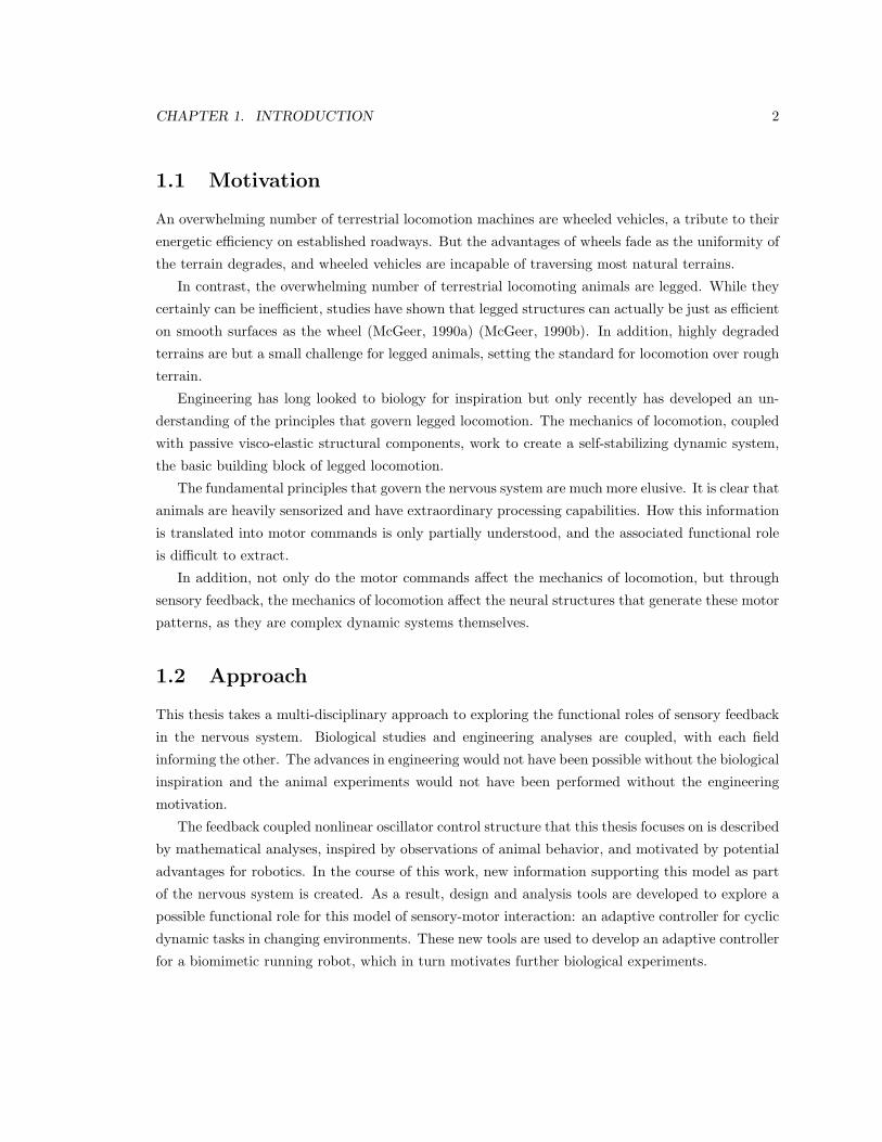
1.1 Motivation
An overwhelming number of terrestrial locomotion machines are wheeled vehicles, a tribute to their
energetic efficiency on established roadways. But the advantages of wheels fade as the uniformity of
the terrain degrades, and wheeled vehicles are incapable of traversing most natural terrains.
In contrast, the overwhelming number of terrestrial locomoting animals are legged. While they
certainly can be inefficient, studies have shown that legged structures can actually be just as efficient
on smooth surfaces as the wheel (McGeer, 1990a) (McGeer, 1990b). In addition, highly degraded
terrains are but a small challenge for legged animals, setting the standard for locomotion over rough
terrain.
Engineering has long looked to biology for inspiration but only recently has developed an un-
derstanding of the principles that govern legged locomotion. The mechanics of locomotion, coupled
with passive visco-elastic structural components, work to create a self-stabilizing dynamic system,
the basic building block of legged locomotion.
The fundamental principles that govern the nervous system are much more elusive. It is clear that
animals are heavily sensorized and have extraordinary processing capabilities. How this information
is translated into motor commands is only partially understood, and the associated functional role
is difficult to extract.
In addition, not only do the motor commands affect the mechanics of locomotion, but through
sensory feedback, the mechanics of locomotion affect the neural structures that generate these motor
patterns, as they are complex dynamic systems themselves.
1.2 Approach
This thesis takes a multi-disciplinary approach to exploring the functional roles of sensory feedback
in the nervous system. Biological studies and engineering analyses are coupled, with each field
informing the other. The advances in engineering would not have been possible without the biological
inspiration and the animal experiments would not have been performed without the engineering
motivation.
The feedback coupled nonlinear oscillator control structure that this thesis focuses on is described
by mathematical analyses, inspired by observations of animal behavior, and motivated by potential
advantages for robotics. In the course of this work, new information supporting this model as part
of the nervous system is created. As a result, design and analysis tools are developed to explore a
possible functional role for this model of sensory-motor interaction: an adaptive controller for cyclic
dynamic tasks in changing environments. These new tools are used to develop an adaptive controller
for a biomimetic running robot, which in turn motivates further biological experiments.
CHAPTER 1. INTRODUCTION 3
1.3 Contributions
The contributions of this thesis are:
• Successful behavioral predictions using a feedback coupled nonlinear oscillator model for high
speed running with a sustained oscillatory perturbation. (Chapter 4)
• Animal experiment results showing the use of sensory feedback at the highest speeds of lo-
comotion and demonstrating behavior consistent with a feedback coupled nonlinear oscillator
model of the neural circuits responsible for motor pattern generation. (Chapter 4)
• A three dimensional visualization tool for designing feedback coupled nonlinear oscillator con-
trollers (Chapter 5)
• An analysis tool for predicting the behavior of a feedback coupled system as dynamic conditions
change and suggesting design modifications (Chapter 5)
• The intentional time delay design technique for tuning the frequency of a feedback coupled
system (Chapter 5)
• A design visualization tool for pulse feedback coupled systems (Chapter 6)
• An adaptive, feedback coupled nonlinear oscillator controller for a biomimetic hexapod running
over different slopes of ±15◦ (Chapter 6)
Taken together, these contributions provide a non ad-hoc, biologically-inspired approach for
achieving adaptive behaviors. While the particular design example here was a biologically-inspired
running robot, the design and analysis tools developed are general, and can be used to design a
feedback coupled nonlinear oscillator controller to produce arbitrary adaptive behaviors for any
cyclic dynamic system.
1.4 Outline
The remainder of this thesis is organized as follows:
Chapter 2 quickly reviews the history of legged robotics, focusing on early dynamic robots and
more recent, biomimetic running machines. Sensory feedback strategies are examined, especially
with regard to schemes involving self-stabilizing runners and feedback coupled nonlinear oscillators.
Chapter 3 introduces the basic characteristics and mathematical principles behind nonlinear
oscillators. Particular attention is given to the ability of these systems to maintain stable oscilla-
tions in the absence of cyclic input, and exhibit selective frequency entrainment when cyclic forcing
functions are applied. To conclude this chapter, the Matsuoka oscillator that is used throughout the
rest of the thesis is introduced.
CHAPTER 1. INTRODUCTION 4
Chapter 4 begins by highlighting some previous experiments involving motor pattern generation
in the nervous system. The feedback coupled nonlinear oscillator is hypothesized as a model of
these motor pattern generators and an experimental method is proposed. Simulated experiments
are used to generate expected results, comparing perturbation and control cases, using directional
statistics to quantify the results. Then, animal experiments are performed and results are discussed,
demonstrating the use of sensory feedback during high speed locomotion and consistency with the
model proposed.
Chapter 5 advances a visual technique for designing feedback coupled nonlinear oscillator con-
trollers. The method is extended by moving into three dimensions, resulting in a more intuitive
representation. Design for changing dynamic conditions is emphasized, and a novel behavior pre-
diction tool is developed, ω contour analysis. In turn, this tool can be used for design; to determine
the feedback properties necessary to generate the desired behavior. Finally, a new coupled system
design tool is developed, the intentional time delay, that is capable of specifying the coupled system
frequency with a high degree of resolution.
Chapter 6 uses the design and analysis tools developed toward an adaptive controller for the
biomimetic hexapedal robot Sprawlita for running up and down slopes of ±15◦. The biomimetic
principles underlying the robot design are described and comparisons with a dynamic simulation of
the robot are made. Using the tools developed in the previous chapter, a pulse coupled feedback
controller is designed for this simulation, and new design visualization tools are developed for this
class of coupled systems. Finally, the performance of the simulated robot running on slopes is
analyzed and compared to the open-loop case, illustrating the effect that the feedback coupled
nonlinear oscillator has on the locomotion.
Chapter 7 concludes this thesis, discussing the contributions made and suggesting directions
for future work.
Chapter 2
Previous work
Small moves, Ellie, small moves.
-Contact, the movie (based on the novel by Carl Sagan)1
The goal of robust and fast legged locomotion over unknown and varied terrain remains unattained.
Over the last 40 years, a significant number of researchers around the world have focused on this
problem and in many cases, substantial advances were made. However, even the most impressive
robots that have been produced are easily humbled by the performance and versatility of almost any
legged animal, emphasizing the need for (and potential direction of) further work.
This chapter reviews some of the early pioneering and groundbreaking work in legged robotics.
This includes the very first robots, Raibert’s dynamic machines, and recent biomimetic robots. The
chapter then concludes with the sensor-based controllers for this last class of machines, including
biologically-inspired methods similar to the ones explored in this thesis.
2.1 History
The promise of legged robotics (with the possible exception of the entertainment industry) is to go
where wheeled and tracked vehicles cannot. Typically, robotic machines are employed in two types
of environments:
1. highly structured industrial environments where precise, repetitive motions are required
2. unstructured exploratory environments where little knowledge about the locale is known and
the task of the robot is to collect more
While fixed robot arms and wheeled robots dominate industrial environs where floors are flat and
obstacles are well-defined, legged robots are much better suited for dealing with the unknown. It1Movie rewrite by Menno Meyjes, Ann Druyan, Carl Sagan, Michael Goldenberg, and Jim V. Hart
5
CHAPTER 2. PREVIOUS WORK 6
is generally accepted in the robotics community that legged machines can deal with much rougher
terrain and larger obstacles than a wheeled vehicle of the same relative size. This is easily verified by
comparing the rough terrain and obstacle traversal performance of a wheeled vehicle and an animal
of the same size.
2.1.1 The first steps
While the concepts of the wheel and wheeled vehicles are relatively ancient and have been around for
thousands of years, only recently has serious thought been put into the idea of a legged mechanism
for locomotion. The first documented work on a legged machine dates back to 1893 when L.A. Rigg
patented his mechanical horse. While there were many purely mechanical walkers in-between (most
of them toys), the world would have to wait until 1966 to see the first computer controlled (and
therefore robotic by most definitions) walking machine, when McGhee and Frank at the University
of South Carolina built the phoney pony (McGhee, 1967). Soon after, R. Mosher at General Electric
built the GE quadruped (Mosher and Liston, 1968), also known as the General Electric Walking
Truck, which was able to surmount various obstacles. More recently, Carnegie Mellon’s Dante II
(Bares and Wettergreen, 1999) achieved the even more formidable task of walking into an active
volcano to collect scientific data.
The vast number of legged robots have met with varying degrees of success. In general, though,
the mechanics of these machines were simple and stability was maintained by never moving fast
enough to violate quasi-static constraints. While this approach worked, the result was that these
machines were incredibly slow; comparable to the pace of a turtle, not a cheetah. One of the
revolutions in legged robotics occurred when one researcher had a novel idea - using the dynamics
of locomotion rather than canceling them out.
2.1.2 Dynamic legged robots
One of the significant revolutions in legged robotics was Raibert’s work on hopping machines during
the 80s and early 90s (Raibert, 1986) (Hodgins and Raibert, 1990) (Koechling and Raibert, 1988).
These robots were the first to fully exploit the dynamics of motion, and their resulting performance
was astounding - while other robots moved at the slow pace of 0.1 bodylengths/second, Raibert’s
machines were able to easily run at speeds of 1-2 bodylengths/second.
The trade off with these particular robots is that computation became required for basic stability.
Simple kinematics were no longer enough to fully describe the operation of the robot as was the
case with statically stable walkers. With only one leg and a small foot, his hoppers characterized
the unstable inverted pendulum and relied upon leg forces and hip torques to maintain stability.
Despite this instability, the control laws that stabilized this system were simpler and more robust
than could be expected. To be sure, the passive compliance and damping present in the air springs
he used helped simplify this control.
CHAPTER 2. PREVIOUS WORK 7
Others since then have exploited dynamics in legged mechanisms, and one of the more well-
known being the passive walker developed by McGeer (McGeer, 1990a)(McGeer, 1990b). Motivated
by human biomechanics, his work was significant because he showed that the passive dynamics of
a legged system were sufficient to produce stable locomotion - only a slight slope was necessary to
overcome frictional losses. In essence, the control and stability of the mechanism was programmed
into the dynamics of the mechanical structure.
In general, though, it is clear that a niche existed which no robots of the day were capable
of fulfilling. With few exceptions, legged robots before the year 2000 were slow and fragile - a
poor combination for legged robots whose sole intention is exploring the unknown. Some machines
were able to cross rough terrain, but only slowly. Other machines could go very fast, but were
not capable of navigating significantly broken terrain. No machines were both fast and able to
go over rough terrain. In addition, most were quite fragile, regularly requiring extensive repair.
The resulting myriad of unfulfilled applications such as demining, urban warfare intelligence, and
planetary exploration called for small, fast, robust robots.
2.1.3 Biomimetic robots
The change of the millennium saw a renewed interest in biologically-inspired robotics, but with a
new slant. Instead of overly complex control strategies coupled to unwieldy platforms, these new
approaches took a different tack - extremely simple control strategies coupled to mechanical struc-
tures with mechanical intelligence designed in. These researchers took their inspiration from nature,
but did not copy it blindly - exact mechanical duplicates are inappropriate given the limitations of
available technologies. Instead, a functional mapping was employed to extract only the principles
relevant to the desired performance.
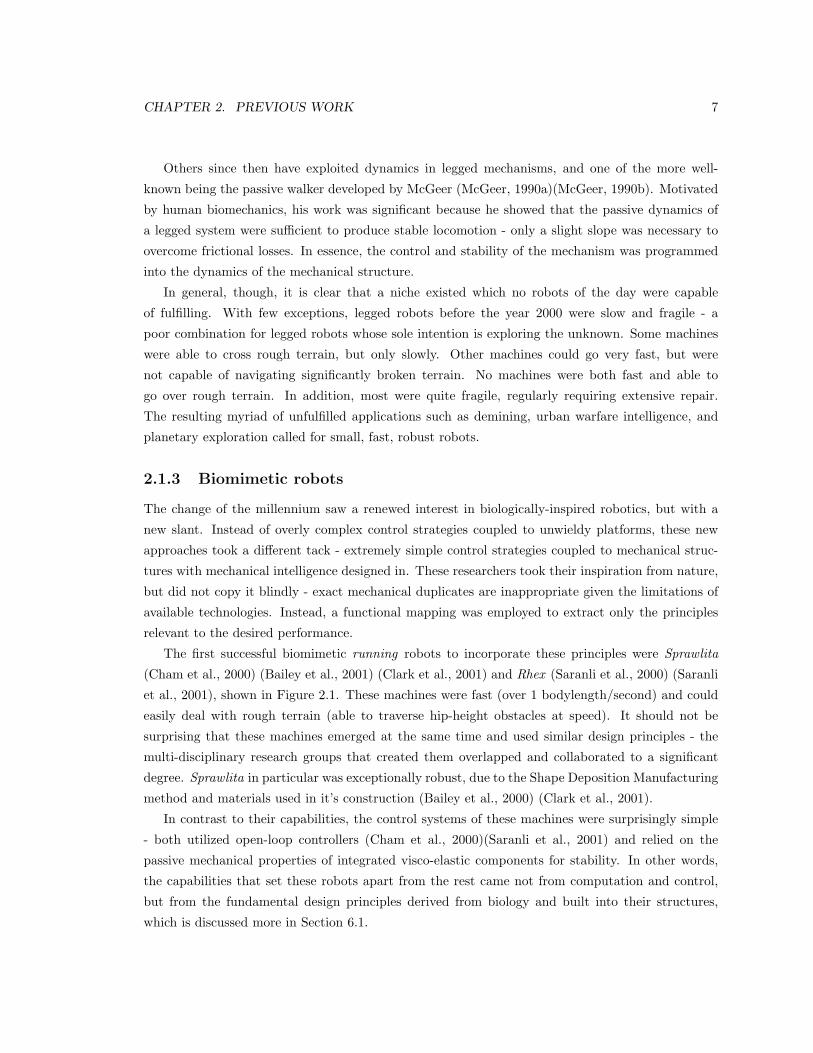
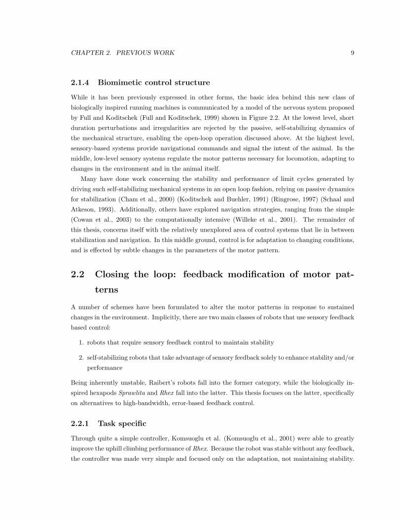
The first successful biomimetic running robots to incorporate these principles were Sprawlita
(Cham et al., 2000) (Bailey et al., 2001) (Clark et al., 2001) and Rhex (Saranli et al., 2000) (Saranli
et al., 2001), shown in Figure 2.1. These machines were fast (over 1 bodylength/second) and could
easily deal with rough terrain (able to traverse hip-height obstacles at speed). It should not be
surprising that these machines emerged at the same time and used similar design principles - the
multi-disciplinary research groups that created them overlapped and collaborated to a significant
degree. Sprawlita in particular was exceptionally robust, due to the Shape Deposition Manufacturing
method and materials used in it’s construction (Bailey et al., 2000) (Clark et al., 2001).
In contrast to their capabilities, the control systems of these machines were surprisingly simple
- both utilized open-loop controllers (Cham et al., 2000)(Saranli et al., 2001) and relied on the
passive mechanical properties of integrated visco-elastic components for stability. In other words,
the capabilities that set these robots apart from the rest came not from computation and control,
but from the fundamental design principles derived from biology and built into their structures,
which is discussed more in Section 6.1.
CHAPTER 2. PREVIOUS WORK 8
a
b
2.5 cm
5 cm
Sprawlita
Rhex
Figure 2.1: The first biomimetic hexapedal robots a) Sprawlita (Cham et al., 2000) (Bailey et al.,2001), b) Rhex (Saranli et al., 2000) (Saranli et al., 2001). Rhex photograph used with permission,Copyright 2004. The Regents of the University of Michigan.
CHAPTER 2. PREVIOUS WORK 9
2.1.4 Biomimetic control structure
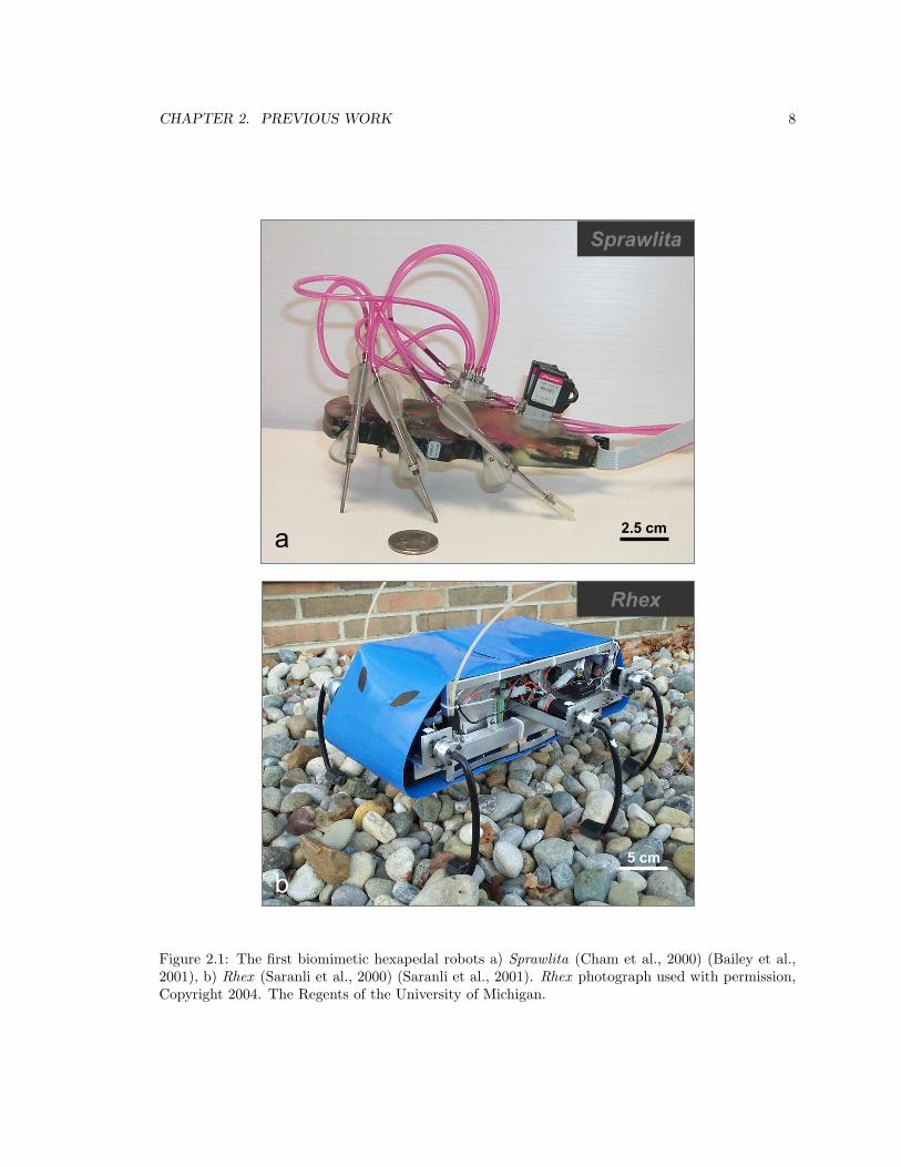
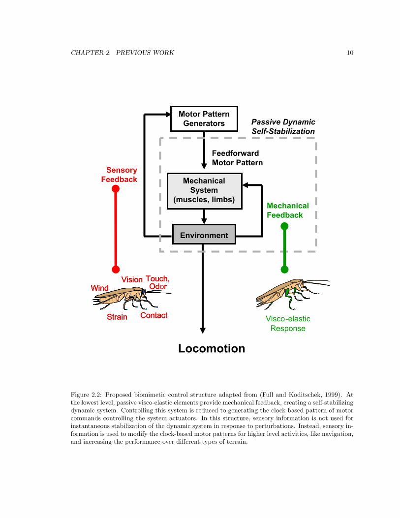
While it has been previously expressed in other forms, the basic idea behind this new class of
biologically inspired running machines is communicated by a model of the nervous system proposed
by Full and Koditschek (Full and Koditschek, 1999) shown in Figure 2.2. At the lowest level, short
duration perturbations and irregularities are rejected by the passive, self-stabilizing dynamics of
the mechanical structure, enabling the open-loop operation discussed above. At the highest level,
sensory-based systems provide navigational commands and signal the intent of the animal. In the
middle, low-level sensory systems regulate the motor patterns necessary for locomotion, adapting to
changes in the environment and in the animal itself.
Many have done work concerning the stability and performance of limit cycles generated by
driving such self-stabilizing mechanical systems in an open loop fashion, relying on passive dynamics
for stabilization (Cham et al., 2000) (Koditschek and Buehler, 1991) (Ringrose, 1997) (Schaal and
Atkeson, 1993). Additionally, others have explored navigation strategies, ranging from the simple
(Cowan et al., 2003) to the computationally intensive (Willeke et al., 2001). The remainder of
this thesis, concerns itself with the relatively unexplored area of control systems that lie in between
stabilization and navigation. In this middle ground, control is for adaptation to changing conditions,
and is effected by subtle changes in the parameters of the motor pattern.
2.2 Closing the loop: feedback modification of motor pat-
terns
A number of schemes have been formulated to alter the motor patterns in response to sustained
changes in the environment. Implicitly, there are two main classes of robots that use sensory feedback
based control:
1. robots that require sensory feedback control to maintain stability
2. self-stabilizing robots that take advantage of sensory feedback solely to enhance stability and/or
performance
Being inherently unstable, Raibert’s robots fall into the former category, while the biologically in-
spired hexapods Sprawlita and Rhex fall into the latter. This thesis focuses on the latter, specifically
on alternatives to high-bandwidth, error-based feedback control.
2.2.1 Task specific
Through quite a simple controller, Komsuoglu et al. (Komsuoglu et al., 2001) were able to greatly
improve the uphill climbing performance of Rhex. Because the robot was stable without any feedback,
the controller was made very simple and focused only on the adaptation, not maintaining stability.
CHAPTER 2. PREVIOUS WORK 10
MechanicalSystem
(muscles, limbs)
Environment
MechanicalFeedback
SensoryFeedback
Motor PatternGenerators
FeedforwardMotor Pattern
Passive DynamicSelf-Stabilization
Locomotion
Wind
Strain Contact
Vision Touch, OdorWind
Strain Contact
Vision Touch, OdorWind
Strain Contact
Vision
Visco-elasticResponse
Touch, Odor
Figure 2.2: Proposed biomimetic control structure adapted from (Full and Koditschek, 1999). Atthe lowest level, passive visco-elastic elements provide mechanical feedback, creating a self-stabilizingdynamic system. Controlling this system is reduced to generating the clock-based pattern of motorcommands controlling the system actuators. In this structure, sensory information is not used forinstantaneous stabilization of the dynamic system in response to perturbations. Instead, sensory in-formation is used to modify the clock-based motor patterns for higher level activities, like navigation,and increasing the performance over different types of terrain.
CHAPTER 2. PREVIOUS WORK 11
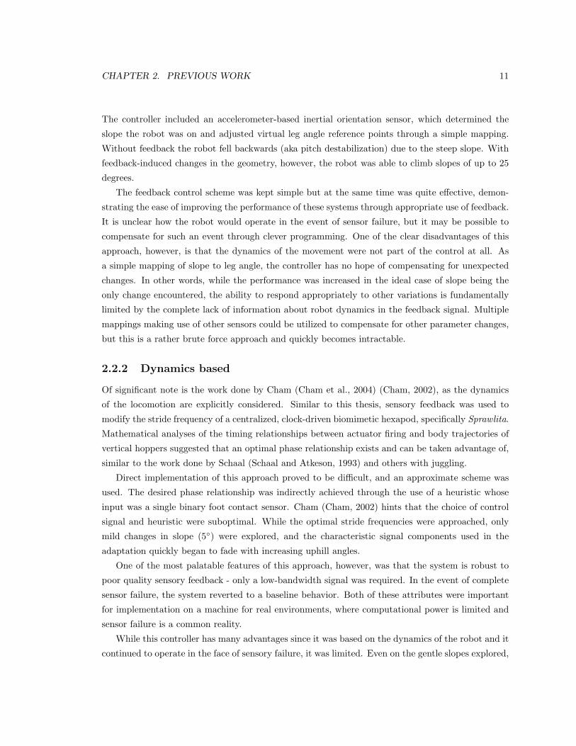
The controller included an accelerometer-based inertial orientation sensor, which determined the
slope the robot was on and adjusted virtual leg angle reference points through a simple mapping.
Without feedback the robot fell backwards (aka pitch destabilization) due to the steep slope. With
feedback-induced changes in the geometry, however, the robot was able to climb slopes of up to 25
degrees.
The feedback control scheme was kept simple but at the same time was quite effective, demon-
strating the ease of improving the performance of these systems through appropriate use of feedback.
It is unclear how the robot would operate in the event of sensor failure, but it may be possible to
compensate for such an event through clever programming. One of the clear disadvantages of this
approach, however, is that the dynamics of the movement were not part of the control at all. As
a simple mapping of slope to leg angle, the controller has no hope of compensating for unexpected
changes. In other words, while the performance was increased in the ideal case of slope being the
only change encountered, the ability to respond appropriately to other variations is fundamentally
limited by the complete lack of information about robot dynamics in the feedback signal. Multiple
mappings making use of other sensors could be utilized to compensate for other parameter changes,
but this is a rather brute force approach and quickly becomes intractable.
2.2.2 Dynamics based
Of significant note is the work done by Cham (Cham et al., 2004) (Cham, 2002), as the dynamics
of the locomotion are explicitly considered. Similar to this thesis, sensory feedback was used to
modify the stride frequency of a centralized, clock-driven biomimetic hexapod, specifically Sprawlita.
Mathematical analyses of the timing relationships between actuator firing and body trajectories of
vertical hoppers suggested that an optimal phase relationship exists and can be taken advantage of,
similar to the work done by Schaal (Schaal and Atkeson, 1993) and others with juggling.
Direct implementation of this approach proved to be difficult, and an approximate scheme was
used. The desired phase relationship was indirectly achieved through the use of a heuristic whose
input was a single binary foot contact sensor. Cham (Cham, 2002) hints that the choice of control
signal and heuristic were suboptimal. While the optimal stride frequencies were approached, only
mild changes in slope (5◦) were explored, and the characteristic signal components used in the
adaptation quickly began to fade with increasing uphill angles.
One of the most palatable features of this approach, however, was that the system is robust to
poor quality sensory feedback - only a low-bandwidth signal was required. In the event of complete
sensor failure, the system reverted to a baseline behavior. Both of these attributes were important
for implementation on a machine for real environments, where computational power is limited and
sensor failure is a common reality.
While this controller has many advantages since it was based on the dynamics of the robot and it
continued to operate in the face of sensory failure, it was limited. Even on the gentle slopes explored,

CHAPTER 2. PREVIOUS WORK 12
the feedback scheme was suboptimal. It is important to note that this approach was inspired mainly
by mathematics not biology. This leads to the question of how such a scheme can be improved by
taking a more biomimetic approach, one that is addressed in the following sections and the rest of
this thesis.
2.3 Nonlinear oscillators for locomotion control
Nonlinear oscillators have been used to model a number of cyclic behaviors observed in animals, rang-
ing from sleep cycles to high-speed locomotion. Drawing on the biomimetic approach, researchers
have explored using nonlinear oscillators as part of a control scheme for walking machines. The
majority of work has focused on control methods that use nonlinear oscillators, but ones that are
not influenced by sensory information. These methods include gait generation and reflex gating
which are discussed in this section.
2.3.1 Inter-limb coordination for gait generation
The most common use of coupled nonlinear oscillators in legged systems is individual leg control
toward the generation of gait. Distributed, one-per-leg, networks of nonlinear oscillators automati-
cally produce recognizable gait patterns, and the gaits possible depend on the pattern of oscillator
interconnections (Matsuoka, 1987) (Cruse et al., 1998). A tonic input, representing the influence of
higher centers, changes the overall excitation level of the system and different gaits spontaneously
emerge. For example, the network may produce a wave gait at low levels of tonic excitation and
an alternating tripod gait at high levels of excitation. This is quite exciting, as controlling such
a complex system is simplified to changing one parameter to get a family of interesting behaviors
(Klavins and Koditschek, 2002)(Cruse et al., 1998).
Interestingly, the research on using oscillators for this type of coordination largely ignores using
sensory feedback from the outside world. Most of the work has been done toward coupling the
output of one leg oscillator to another leg oscillator, not coupling the resulting dynamic actions of
the mechanical system back to the oscillators. As such, these control systems produce coordinated
motor commands, but are unaware of the resulting performance and are essentially open-loop. One
notable exception is the work of Klavins (Klavins and Koditschek, 2002), who explored using sensory
feedback to drive the leg oscillators, in fact creating a system similar to the ones described in section
2.4. However, the bulk of the study referred to the stability of the gait, and talked little about the
effect on performance in response to changes in external conditions.

CHAPTER 2. PREVIOUS WORK 13
2.3.2 Reflex gating
An alternative role of nonlinear oscillators is to gate sensory information (Lewis, 2002). While not
the commonly held view, the cerebellum has been hypothesized to play a sensory coordination role
rather than a motor one, based on rat whisker sensorization studies (Bower, 1997) (Mauk et al.,
2000). In fact, a cerebellar-like structure in fish has been shown to cancel out self-generated stimuli
(Lewis, 2002). The basic idea stems from research on decerebate cats in which a stimulus during
one phase of the locomotion produces a different response than the same stimulus during a different
phase of the locomotion (Duenas et al., 1990).
Similarly, Lewis proposes that for robotics the appropriate reaction to sensory input, should be
gated by the output of the oscillator that is driving the mechanical system. The result is that different
control laws are used during swing and stance phases of the leg and the switching is controlled by
the state of the internal oscillator. Thus, the nonlinear oscillator is not used as an explicit part of
generating the reaction itself, but instead as a routing method to determine when and how sensory
feedback is used. In this case, the nonlinear oscillator is involved in the response generation, but
indirectly. The following section discusses explicitly involving the nonlinear oscillator in generating
responses to sensory information, this time as an integral part of a coupled dynamic system.
2.4 Feedback coupling a nonlinear oscillator
As discussed in the previous section (2.3), nonlinear oscillators have been used to model a number
of cyclic behaviors observed in animals. In contrast to the structures discussed there, however,
one of the most notable aspects of the behaviors observed is that they are generally influenced by
external stimuli. This sensory-based influence on the cyclic motor patterns generated is a rich and
important behavior, and one that is explored mathematically and experimentally in Chapters 3 and
4, respectively.
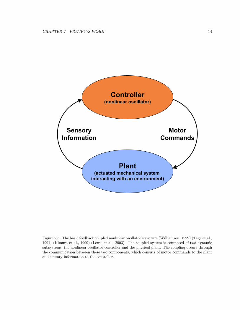
As such, a feedback coupled nonlinear oscillator is explicitly influenced by sensory feedback and
involved in generating responses to this information. The structure of a feedback coupled nonlinear
oscillator system is shown in Figure 2.3 and is composed of two parts, the nonlinear oscillator
controller and the physical plant. Each component has its own set of dynamics, but through the
sensory information and motor commands communicated between them, the subsystems are coupled
together. As a result, the coupled system behavior is quite different than the behavior of each
component in isolation.
When a feedback coupled nonlinear oscillator is used as shown in Figure 2.3, there are several
advantageous features, as listed here:
1. works with the dynamics of the mechanical system, not isolated from them
2. is robust to sensor failure (oscillates without sensory feedback)
CHAPTER 2. PREVIOUS WORK 14
Controller(nonlinear oscillator)
Plant(actuated mechanical system
interacting with an environment)
MotorCommands
SensoryInformation
Figure 2.3: The basic feedback coupled nonlinear oscillator structure (Williamson, 1999) (Taga et al.,1991) (Kimura et al., 1999) (Lewis et al., 2003). The coupled system is composed of two dynamicsubsystems, the nonlinear oscillator controller and the physical plant. The coupling occurs throughthe communication between these two components, which consists of motor commands to the plantand sensory information to the controller.

CHAPTER 2. PREVIOUS WORK 15
3. can filter out extraneous sensory information (from noise and disturbances)
4. has low computational requirements (has even been implemented in analog hardware (Lewis
et al., 2000))
5. establishes a general structure for designing controllers for cyclic dynamic behaviors (not ad-
hoc)
The last point is an important one, as it emphasizes the usefulness of the biomimetic approach.
Like the task-specific and dynamics-based schemes listed above, many robot controllers are very
specific, usually to both the robot and the environment. In other words, these schemes work for
the specific case for which they were designed, but they do not represent a general approach. In
contrast, nonlinear oscillators are used to model nervous system behavior for a wide range of sensory
influenced activities, even including high-speed locomotion (Chapter 4). In fact, almost every cyclic
motor activity can be modeled as being controlled by a nonlinear oscillator (van der Pol and van der
Mark, 1928), indicating that this is a very general structure, one that can be used in robotics for
feedback controlling any type of cyclic dynamic activity.
How to design such coupled systems is an area of research that has not been well explored. Lewis
(Lewis et al., 2003) successfully implemented a stabilizing controller for a planar bipedal runner, but
the rationales for the design choices made are unclear. Williamson (Williamson, 1999) developed
a visual technique for predicting the behavior of a coupled system, but he did not focus on tools
for adaptation in response to changing conditions. Others (Zhang et al., 2003) (Fukuoka et al.,
2003) (Kimura et al., 1999) have implemented adaptive controllers for locomoting robots, but only
in conjunction with other sensory-based components, and the relative contribution is difficult to
discern. With the exception of the Williamson design method, which is discussed extensively in
Chapter 5, each one of these approaches is detailed here.
2.4.1 Ring rules for stability
As discussed before, some legged systems are unstable and require some sort of sensory feedback just
to keep from crashing. One example of such a system is the planar biped that Lewis et al. (Lewis
et al., 2003) built for running on an inertial treadmill. They explored using a coupled nonlinear
oscillator system to stabilize an unstable mode of this biped, the angular tilt of the runner in the
sagittal plane. Using a design method called Ring Rules (Lewis, 1996), they were able to design a
coupled system that stabilized the tilt of the entire biped. The knee joint angle, hip joint angle,
and ground reaction forces were used as inputs to the nonlinear oscillator, which set the hip joint
extrema switching points for the locomotion. Additionally, the digital computational power needed
to operate this robot was zero - everything was implemented in analog electronics. In fact, VLSI
techniques were used and the entire oscillator was built on one chip (Lewis et al., 2000).
CHAPTER 2. PREVIOUS WORK 16
Interestingly, Lewis was able to show graphically the action of the nonlinear oscillator and how
the coupled system trapped the robot tilt angle within a certain region of values. Unfortunately,
however, the reasoning behind the steps taken to design the coupled system are unclear, and it is
difficult to see how this method can be distilled into a general design approach. Without design tools
to guide the selection of parameter values, establishment of adaptive rules, and choice of feedback,
the approach seems limited to design through experimentation.
2.4.2 Adaptation to uneven terrain
In many studies uneven terrain is modeled by changing the slopes, and the nonlinear oscillator
controlled system is tested on these surfaces as an afterthought to quantify robustness (Taga et al.,
1991) (Taga, 1995). Kimura and his colleagues (Zhang et al., 2003) (Fukuoka et al., 2003) (Kimura
et al., 1999), however, explored controlling a robot with a feedback coupled nonlinear oscillator
specifically for walking on uneven terrain. Using vestibular and hip angle feedback, they were able
to get their quadrupedal robot Patrush to traverse short (1 body length) slopes of ±12◦, 3 centimeter
high obstacles, and terrain undulations.
Unfortunately, the mechanism by which the feedback improved the performance in the different
types of terrain is hard to distill from their results. In addition to the nonlinear oscillator, sensory
information was supplied to pre-programmed reflexes. As a result, the relative contributions of one
feedback system versus the other are difficult to discern. Kimura does hint, however, that phase
relationships are what play the crucial role as the phase differences between the rolling motion of
the body and the pitching of the legs seem to be the important regulating effect.
While the results of these experiments are exciting and encouraging, a thorough understanding
of the exact mechanisms responsible for the improved performance and how to design them was not
established through this work. Again, the rationale for the design choices made is not well explained
and seems to come from experimental parameter tuning, not as part of a methodical design approach.
2.5 Summary
In summary, there continues to be room for progress with legged locomotion systems. Once the
first steps of robotic legged locomotion took place, researchers like Raibert (Raibert, 1986) quickly
learned that the dynamics of locomotion were important. Incorporating these dynamics and other
fundamental biological principles, biomimetic robots broke speed and rough terrain traversal records
with their self-stabilizing operation. Feedback-based controllers for these robots were free from
concerns about stabilization, but still needed to work with the dynamics of locomotion to be effective.
Biologically inspired controllers, such as feedback coupled nonlinear oscillators, have many fea-
tures, including explicit use of sensory feedback combined with robustness to complete sensor failure.
These systems take the dynamics of cyclic behaviors such as locomotion into account, and represent
CHAPTER 2. PREVIOUS WORK 17
a potential control scheme for these systems in general. In experimental robot studies, these con-
trollers have shown the ability to act as adaptive controllers, generating different motor commands
and increasing robot performance in the face of changing environmental conditions.
How these controllers work toward creating this adaptive behavior is not well understood, espe-
cially when they are used in conjunction with other feedback-based strategies. In addition, while
these structures work, no methodical design process exists outlining the steps that are taken and
tools available during the formulation of these feedback coupled nonlinear oscillators.
Chapters 5 and 6 address this shortcoming in the literature. Chapter 5 details a design method
and develops tools for creating adaptive coupled systems. Chapter 6 uses these tools toward a specific
example, designing an feedback coupled nonlinear oscillator adaptive controller for the biomimetic
hexapod, Sprawlita, running up and down slopes. The motivation for this approach comes from
animal experiments that explore feedback coupled oscillatory behavior, performed as part of this
thesis and described in Chapter 4. First, however, the mathematics of nonlinear oscillators are
reviewed in Chapter 3, providing a theoretical foundation for the animal experiments and design
procedures carried out.
Chapter 3
Nonlinear oscillators
The cycles of life are ultimately biochemical in mechanism, but many of the principles
that dominate their orchestration are essentially mathematical.
-Arthur T. Winfree (The Geometry of Biological Time)
The world, and the systems in it, are, of course, nonlinear. Nonetheless, there has been an
enormously successful practice of engineering in linearizing systems and applying the powerful tools
of linear mathematical analysis to them. Where this basic approach fails is where the nonlineari-
ties themselves are of particular interest. This thesis is concerned with one such class of systems,
nonlinear oscillators.
Nonlinear oscillators have many characteristics, but the ones that are relevant to this work are:
1. self-sustained limit cycle generation in the absence of cyclic input
2. selective entrainment when cyclic inputs are present
Both of these attributes are fundamentally nonlinear, and cannot be represented by linear systems.
In addition, these are also the characteristics that make nonlinear oscillators, as part of coupled
systems as discussed in the last chapter, so attractive as controllers for dynamic mechanical systems
such as running animals and robots.
When the sensors are working, they relay information about the cyclic dynamics of the mechanical
system through the feedback coupling, entraining the nonlinear oscillator to these dynamics which
in turn generates appropriate motor commands. While the nonlinear oscillator dynamics are always
influenced by this feedback, they also have the ability to selectively disregard signals that fall outside
the relevant frequency spectrum. Through this selective entrainment, sensory information far from
the cycle frequency is considered spurious and is largely rejected.
In addition, oscillations persist in the event of sensor failure. The nonlinear oscillators explored
here generate self-sustained limit cycles, and continue to oscillate in the absence of cyclic input
18
CHAPTER 3. NONLINEAR OSCILLATORS 19
through the feedback coupling. While the advantages of the feedback coupling are lost in these
situations, continued open-loop operation is preferred to nonfunctionality.
This chapter begins by quickly reviewing the history of nonlinear oscillators, and introducing two
basic examples. Then, the differences between linear and nonlinear oscillators are discussed briefly,
with an emphasis on points relevant to the fundamental characteristics, discussed above, that are of
interest to this thesis. Finally, this chapter concludes with nonlinear oscillators that have been used
to model individual neurons and interconnected networks of these neurons, motivating the animal
experiments that investigate feedback coupled oscillatory behavior in cockroaches during high-speed
locomotion. The nonlinear oscillator focused on for these experiments and later in Chapters 5 and 6 is
the Matsuoka oscillator (Matsuoka, 1985) (Matsuoka, 1987), a popular model of such interconnected
neuron networks.
3.1 A short history
Nonlinear oscillators have been used to model a wide variety of physical phenomena, including
electrical circuits, mechanical pendula, buckling beams, predator prey populations, and musical
instruments (Sastry, 1999). While it may be surprising that such different systems can be represented
by the same model, nonlinear oscillators are adept at capturing the rich behavior of many types of
physical systems.
3.1.1 The van der Pol oscillator
While work had definitely been done with nonlinear oscillators before then, van der Pol’s analysis of
electronic circuits and heartbeat anomalies in the 1920’s is generally regarded as the first significant
work modeling biological phenomena with nonlinear oscillators (van der Pol and van der Mark,
1928). van der Pol was interested in the anomalies in heartbeat, or arrhythmias. Heartbeats have
their own rhythm, but can be easily influenced by external stimuli. He found that he could model the
system that generates these heartbeats with a nonlinear oscillator, which has similar characteristics.
Slightly modified here, the basic equation of the nonlinear oscillatory he used (which has since
been named the van der Pol oscillator) is:
x + ε(x2 − 1)x + x = 0 (3.1)
where x and x describe the state of the system. ε is always positive and is the coefficient of the
resistance present in the system. This resistance is negative for small amplitudes of x, as given by
x2− 1, and is responsible for generating the self-sustained limit cycle operation as discussed later in
section 3.2.1.
CHAPTER 3. NONLINEAR OSCILLATORS 20
3.1.2 The Rayleigh oscillator
Rayleigh also investigated various physical phenomena and modeled their characteristics using non-
linear oscillators. Although he carried out a number of experiments involving other musical instru-
ments (Rayleigh, 1887), his modeling of the clarinet reed in response to sustained blowing is quite
well known. It is interesting to note that with such instruments, the input necessary to generate
such oscillations is itself not oscillatory - highlighting that even this basic component of the behavior
can not be modeled by a linear system.
Modified slightly here, the he used the following equation to model the blowing of a clarinet reed,
and it is typically called the Rayleigh oscillator:
x + ε(x2 − 1)x + x = 0 (3.2)
The coefficients of the various state variables can be used for different clarinet characteristics, such
as stiffer reeds and more intense blow forces (Sastry, 1999). x and x again describe the state of the
system, and ε describes the resistance present. As with the van der Pol oscillator, this resistance
can be negative which generates self-sustained limit cycle oscillations, but in this case for small
amplitudes of x, not x. Confusingly, this is also sometimes called the van der Pol oscillator in some
texts, likely due to the fact that the two are related. Differentiating the equation for the Rayleigh
oscillator and setting x = x yields the equations for the van der Pol oscillator.
3.2 Nonlinear oscillator characteristics
While not all nonlinearity oscillators are as simple as the van der Pol and Rayleigh oscillators, most
have very similar fundamental characteristics which separate them from linear oscillators. Some of
the interesting behaviors that are unique to nonlinear oscillators include multiple equilibrium points,
bifurcations, chaos, jump resonance, subharmonic generation , and asynchronous quenching (Slotine
and Li, 1991). However, the characteristics of nonlinear oscillators that are relevant to this thesis
are self-sustained limit cycles generation and selective entrainment. In this section, the van der Pol
oscillator will be used as an example to demonstrate these two principles.
3.2.1 Self-sustained limit cycle generation
In the description of the Rayleigh oscillator above in section 3.1.2, it was noted that the clarinet reed
oscillated in response to a steady input, a constant stream of air. In general, nonlinear oscillators
can be used to model physical systems that generate oscillations by drawing from a constant energy
source (van der Pol and van der Mark, 1928), rather than a cyclic one. The term self-sustained
limit cycles refer to the ability of a nonlinear oscillator to maintain a stable oscillatory motion in
the absence of an oscillatory input. This is a fundamentally nonlinear behavior, as linear systems
CHAPTER 3. NONLINEAR OSCILLATORS 21
are not capable of maintaining stable oscillatory motions without an oscillatory input of the same
frequency.
As it lends itself to easy understanding, the van der Pol oscillator, repeated here from Section
3.1.1, is used as an example to illustrate the basic mechanism of self-sustained limit cycles:
x + ε(x2 − 1)x + x = 0 (3.3)
Structurally, this is not much different than a 2nd order linear differential equation. This type of
linear equation can be used to describe a mechanical mass-spring-damper oscillatory system:
x + bx + x = 0 (3.4)
where the coefficients corresponding to the mass and spring constant are omitted as they are assumed
to have a magnitude of 1. The only difference between the two equations, then, is the coefficient of
the x term, but this makes a large difference in the character of the two systems.
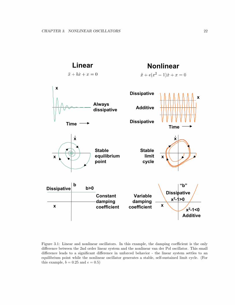
The linear 2nd order system has a special case where b = 0, which corresponds to an unforced
spring-mass system without damping. This linear system oscillates continually as a result of energy
being exchanged between kinetic and potential forms in the mass and spring, respectively. This is
not a stable oscillation, however, as any disturbance to this system results in a permanent change
in the amplitude of the output.
For stable versions of these unforced linear systems, however, the x coefficient b, representing the
damping, is always positive (b > 0 ) and continually dissipates energy, as shown in Figure 3.1. This
energy dissipation stabilizes the system, but also eventually brings it to rest and leads to a stable
fixed point solution at x = 0. x = 0 is an equilibrium point, as the equivalent spring force there is
zero and the x term remains dissipative.
In contrast, the corresponding b term in the van der Pol oscillator, ε(x2 − 1), has the ability to
change sign, dissipating energy at large amplitudes (x > 1) but generating energy at small amplitudes
(x < 1), which is shown in Figure 3.1. In effect, the system oscillates because the equilibrium point
at x = 0 is unstable because the x term is negative. While the system does remain at rest if x, x = 0,
any deviation from this equilibrium point is amplified and results in oscillations. The oscillations are
limited and the limit cycle is stable because ε(x2−1) changes sign for large amplitudes and becomes
dissipative. Therefore, the amplitude of the resulting oscillation is a balance between these regions
of energy addition and dissipation. Once this balance is reached, the nonlinear system maintains
these stable oscillations at a fixed frequency, thereby generating self-sustained limit cycles.
This is not only interesting, but it is also important from a control perspective. In the event
of complete sensor failure, a feedback coupled nonlinear oscillator controller continues to cycle and
produce usable motor commands as a result of the self-sustained limit cycle generation. Stable limit
cycles could also be generated by a forced linear oscillator, but this is quite a different phenomenon
CHAPTER 3. NONLINEAR OSCILLATORS 22
NonlinearLinear
Always dissipative
Time
x
x
b
Stableequilibriumpoint
Constantdampingcoefficient
x.
x
Additive
Dissipative
Dissipative
Stablelimit
cycle
Variabledamping
coefficient
b>0
x2-1<0
x2-1>0x
x
Time
x.
x
Additive
Dissipative“b”Dissipative
Figure 3.1: Linear and nonlinear oscillators. In this example, the damping coefficient is the onlydifference between the 2nd order linear system and the nonlinear van der Pol oscillator. This smalldifference leads to a significant difference in unforced behavior - the linear system settles to anequilibrium point while the nonlinear oscillator generates a stable, self-sustained limit cycle. (Forthis example, b = 0.25 and ε = 0.5)
CHAPTER 3. NONLINEAR OSCILLATORS 23
as this linear oscillator can never not oscillate at that frequency.
If a linear oscillator is forced in this way to generate self-sustained oscillations for the event of
sensor failure, complete entrainment to the natural dynamics of a mechanical system when feedback
is present becomes impossible. Therefore, with a linear oscillator a choice must be made between
the robustness to sensor failure and the ability to take advantage of sensory feedback. Fortunately,
nonlinear oscillators which generate self-sustained limit cycles also respond to cyclic external inputs,
but in a fundamentally different way which does not necessitate that this choice be made.
3.2.2 Selective entrainment
The terms entrainment (Jordan and Smith, 1999) and synchronization (Minorsky, 1962) are only
slightly different. Synchronization refers to the event of two systems of slightly different frequencies
falling into a common rhythm through mutual coupling. Entrainment, however, refers to one oscil-
lator being forced at a fixed frequency, and cycling at that frequency as a result. Later, in Chapter
5, it will be shown that the design method utilizes entrainment, but the two components of the
coupled system produced operate in synchronization.
Like linear oscillators, nonlinear oscillators can be entrained to cyclic external inputs, also called
forcing functions. Therefore, either type of oscillator can work with the dynamics of the mechanical
system through feedback coupling. The difference between the two oscillators, though, is how they
respond to these inputs, as nonlinear oscillators are selective about the cyclic inputs they can be
entrained to.
Once they have reached steady state, linear oscillators always cycle at the frequency at which
they are forced. They are entrained to the input regardless of the forcing function frequency and
amplitude, or the natural frequency of the linear system itself. This is an important consequence
of the superposition principle, which only applies to linear systems and will be discussed more in
Section 5.1.1.
Nonlinear oscillators, however, do not adhere to this principle and do not always cycle at the
frequency of the input. In this way, they are more selective in how they are entrained. The oscillations
resulting from a forced nonlinear oscillator depend on the frequency of the forcing function relative
to the self-sustained limit cycle frequency of the nonlinear oscillator and the amplitude of the cyclic
input. The result of this selective entrainment has been well documented (Jordan and Smith, 1999)
(Wever, 1960) (Williamson, 1999) and is most often characterized by two plots - the frequency
entrainment and resonance tongue plots.
Frequency entrainment plot
The difference in how linear and nonlinear oscillators respond to external inputs is clear in the
frequency entrainment plots, shown in Figure 3.2. In these plots, the frequency of the oscillator is
plotted against the frequency of the external forcing function. If the cyclic external input determines
CHAPTER 3. NONLINEAR OSCILLATORS 24
the oscillator frequency, then the oscillator is entrained and there is a constant ratio relationship
between the frequencies.
In the case of a linear oscillator, the frequency of the external input strictly determines the steady
state frequency of the oscillator, regardless of the unforced natural frequency of the oscillator. This
is an important consequence of superposition, a concept that will be described in more detail in
Section 5.1.1. As shown in the figure, the relationship between the two signals is a line of slope 1,
indicating consistent entrainment over all frequencies.
In contrast, the nonlinear oscillator shown in Figure 3.2 exhibits selective frequency entrainment.
The 1:1 relationship between the oscillations and the forcing function does exist, but only in a specific
region (Wever, 1960) (Sastry, 1999). In other regions, the input still acts on and affects the system,
but does not determine the fundamental frequency of the oscillation.
The only exception to this are regions around the harmonics of the self sustained limit cycle
frequency. Interestingly, only the odd harmonics (n = 3, 5, 7, ...) result in oscillator entrainment
for the van der Pol oscillator. For reasons discussed by others (Jordan and Smith, 1999), the even
harmonics (n = 2, 4, 6, ...) do not cause entrainment. For the same reasons, the odd subharmonics
should cause entrainment, but the effect was not noticeable in these simulations. Additionally,
although the entrainment at only the odd harmonics seems to be more typical, it should be noted
that some nonlinear oscillators do show entrainment at all harmonics (Wever, 1960).
It is important to note that there is no magic here and the rules of mathematics still apply. The
nonlinear oscillators are affected by the cyclic inputs in all cases, but internal mechanisms make the
oscillator more sensitive to some frequencies than others. This sensitivity grows with the strength
of the external input, which determines the range over which entrainment occurs as is shown in the
resonance tongue plot.
Resonance tongue plot
In addition to being dependent on the frequency of the forcing function relative to the self-sustained
limit cycle frequency, entrainment is also dependent on the amplitude of the forcing function. In
general, as the amplitude of the forcing function increases, the range around the self-sustained limit
cycle frequency in which synchronization occurs also increases.
The resonance tongue plot is a common way of visualizing this relationship. As shown in Figure
3.3, the minimum input amplitude necessary for entrainment varies as the forcing function frequency
changes. It is clear why these plots are often referred to as resonance tongue plots, as the necessary
input amplitude grows as the distance from the self-sustained limit cycle frequency of the nonlinear
oscillator increases, resulting in a characteristically tongue-like shape.
The van der Pol and Rayleigh oscillators are good basic examples that exhibit the fundamental
nonlinear oscillator behaviors, specifically self-sustained limit cycle generation and selective entrain-
ment. More complex nonlinear oscillators that are used to capture other, detailed behaviors also
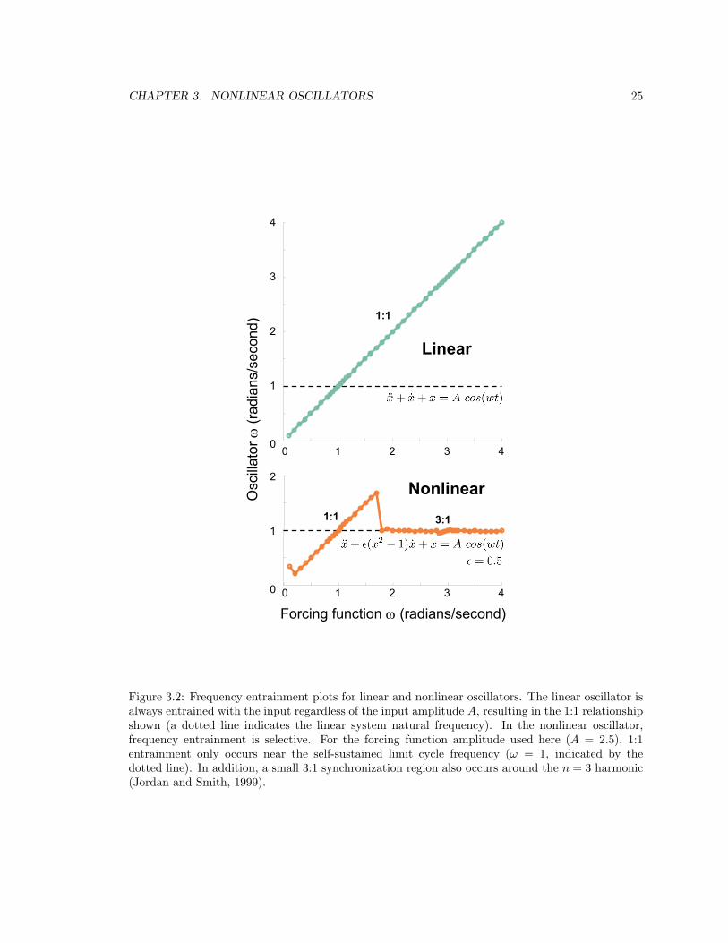
CHAPTER 3. NONLINEAR OSCILLATORS 25
00
1
2
Crop special 2.2
Usual crop is top and bottom: 2.3375Left and right: 1.4375
0 1 2 3 40
1
2
3
4
Osc
illato
r ω(ra
dian
s/se
cond
)
0 1 2 3 4
Forcing function ω (radians/second)
0
1
2Nonlinear
Linear
1:1
1:1 3:1
Figure 3.2: Frequency entrainment plots for linear and nonlinear oscillators. The linear oscillator isalways entrained with the input regardless of the input amplitude A, resulting in the 1:1 relationshipshown (a dotted line indicates the linear system natural frequency). In the nonlinear oscillator,frequency entrainment is selective. For the forcing function amplitude used here (A = 2.5), 1:1entrainment only occurs near the self-sustained limit cycle frequency (ω = 1, indicated by thedotted line). In addition, a small 3:1 synchronization region also occurs around the n = 3 harmonic(Jordan and Smith, 1999).
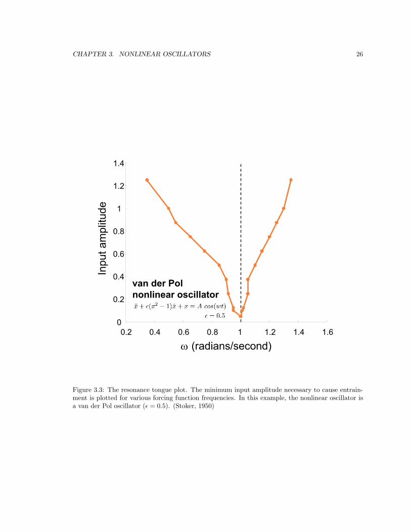
CHAPTER 3. NONLINEAR OSCILLATORS 26
0.2 0.4 0.6 0.8 1 1.2 1.4 1.60
0.2
0.4
0.6
0.8
1
1.2
1.4
ω (radians/second)
Inpu
t am
plitu
de
van der Polnonlinear oscillator
Crop special 2.2
Usual crop is top and bottom: 2.3375Left and right: 1.4375
Figure 3.3: The resonance tongue plot. The minimum input amplitude necessary to cause entrain-ment is plotted for various forcing function frequencies. In this example, the nonlinear oscillator isa van der Pol oscillator (ε = 0.5). (Stoker, 1950)
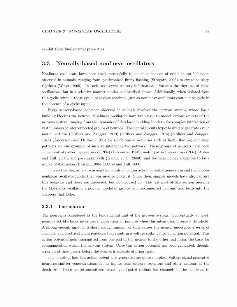
CHAPTER 3. NONLINEAR OSCILLATORS 27
exhibit these fundamental properties.
3.3 Neurally-based nonlinear oscillators
Nonlinear oscillators have been used successfully to model a number of cyclic motor behaviors
observed in animals, ranging from synchronized firefly flashing (Strogatz, 2003) to circadian sleep
rhythms (Wever, 1965). In each case, cyclic sensory information influences the rhythms of these
oscillations, but in a selective manner similar as described above. Additionally, when isolated from
this cyclic stimuli, these cyclic behaviors continue, just as nonlinear oscillators continue to cycle in
the absence of a cyclic input.
Every sensory-based behavior observed in animals involves the nervous system, whose basic
building block is the neuron. Nonlinear oscillators have been used to model various aspects of the
nervous system, ranging from the dynamics of this basic building block to the complex interaction of
vast numbers of interconnected groups of neurons. The neural circuits hypothesized to generate cyclic
motor patterns (Grillner and Zangger, 1979) (Grillner and Zangger, 1975) (Grillner and Zangger,
1974) (Andersson and Grillner, 1983) for synchronized activities such as firefly flashing and sleep
patterns are one example of such an interconnected network. These groups of neurons have been
called central pattern generators (CPGs) (Delcomyn, 1980), motor pattern generators (PGs) (Abbas
and Full, 2000), and pacemaker cells (Kandel et al., 2000), and the terminology continues to be a
source of discussion (Bassler, 1986) (Abbas and Full, 2000).
This section begins by discussing the details of neuron action potential generation and the famous
nonlinear oscillator model that was used to model it. Since then, simpler models have also capture
this behavior and these are discussed, but not focused on. The last part of this section presents
the Matsuoka oscillator, a popular model of groups of interconnected neurons, and leads into the
chapters that follow.
3.3.1 The neuron
The neuron is considered as the fundamental unit of the nervous system. Conceptually at least,
neurons act like leaky integrators, generating an impulse when this integration crosses a threshold.
A strong enough input in a short enough amount of time causes the neuron undergoes a series of
chemical and electrical chain reactions that result in a voltage spike, called an action potential. This
action potential gets transmitted from one end of the neuron to the other and forms the basis for
communication within the nervous system. Once this action potential has been generated, though,
a period of time passes before the neuron is capable of firing again.
The details of how this action potential is generated are quite complex. Voltage signal generated
neurotransmitter concentrations act as inputs from sensory receptors and other neurons at the
dendrites. These neurotransmitters cause ligand-gated sodium ion channels in the dendrites to

CHAPTER 3. NONLINEAR OSCILLATORS 28
open, changing the voltage across the neuron cell membrane and effectively integrating the inputs
over time.
If the amount of neurotransmitter is too low, the sodium ions do not build up enough voltage
and the neuron does not fire. If the membrane voltage changes sufficiently, though, other more
effective voltage-gated sodium ion channels open, resulting in a threshold-based change in behavior.
Because these voltage-gated ion channels are much more effective, the cell membrane potential
changes rapidly, resulting in a large voltage spike that is the action potential. This voltage spike
travels from the soma to the end of the axon, where it links and communicates with other parts of
the neuromuscular system, such as muscles and other neurons.
After the action potential occurs, the cell requires an amount of time to recover before it can
fire again, called the refractory period (Kandel et al., 2000). This recovery occurs as the result of
potassium ions slowly flowing back into the cell and re-establishing the original membrane voltage.
As a result of the leaky integration leading up to the action potential and the refractory period
afterward, the neuron can only be driven by inputs within a frequency range. This frequency selective
entrainment is not unlike the characteristic behavior of the nonlinear oscillators as described in
section 3.2.2. Therefore, it should not be surprising that the first model that successfully captured
the intricacies of neuron action potential generation dynamics was nonlinear.
3.3.2 The Hodgkin-Huxley neuron model
The importance of modeling the neuron and the action potential is evident by the 1963 Nobel prize
in medicine awarded to Hodgkin and Huxley (Hodgkin, 1951) (Hodgkin and F., 1952b) (Hodgkin
and F., 1952a). For this work, they used a squid giant axon preparation to measure membrane
potentials and ionic currents, and modeled these currents with a 4th order nonlinear system. The
ionic currents they modeled are directly responsible for the action potential behavior, as discussed
above.
However, the nonlinear system they used to describe the behavior is quite complex, as it is
a 4th order set of equations with many parameters to tune. Since then, many researchers have
worked toward capturing the basic behavior of the neuron with a simpler, lower order models.
Fitzhugh (Fitzhugh, 1961) and Nagumo (Nagumo et al., 1960) formulated some of the first 2nd
order simplifications of the Hodgkin-Huxley model. There are also 3rd order models (Ghigliazza
and Holmes, 2003) and models with very large numbers of state variables (Grillner, 1999) (Kozlov
et al., 2003). The difference between these various models is how well the intricacies (such as the
individual ion currents) of the neuron behavior are captured. However, it is generally accepted that
the gross behavior is captured in the 2 variable models, such as the Matsuoka oscillator.
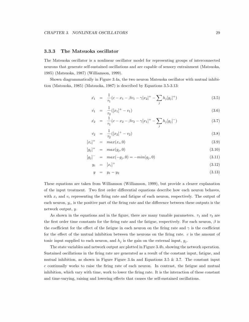
CHAPTER 3. NONLINEAR OSCILLATORS 29
3.3.3 The Matsuoka oscillator
The Matsuoka oscillator is a nonlinear oscillator model for representing groups of interconnected
neurons that generate self-sustained oscillations and are capable of sensory entrainment (Matsuoka,
1985) (Matsuoka, 1987) (Williamson, 1999).
Shown diagrammatically in Figure 3.4a, the two neuron Matsuoka oscillator with mutual inhibi-
tion (Matsuoka, 1985) (Matsuoka, 1987) is described by Equations 3.5-3.13:
x1 =1τ1
(c− x1 − βv1 − γ[x2]+ −∑
j
hj [gj ]+) (3.5)
v1 =1τ2
([x1]+ − v1) (3.6)
x2 =1τ1
(c− x2 − βv2 − γ[x1]+ −∑
j
hj [gj ]−) (3.7)
v2 =1τ2
([x2]+ − v2) (3.8)
[xi]+ = max(xi, 0) (3.9)
[gj ]+ = max(gj , 0) (3.10)
[gj ]− = max(−gj , 0) = −min(gj , 0) (3.11)
yi = [xi]+ (3.12)
y = y1 − y2 (3.13)
These equations are taken from Williamson (Williamson, 1999), but provide a clearer explanation
of the input treatment. Two first order differential equations describe how each neuron behaves,
with xi and vi representing the firing rate and fatigue of each neuron, respectively. The output of
each neuron, yi, is the positive part of the firing rate and the difference between these outputs is the
network output, y.
As shown in the equations and in the figure, there are many tunable parameters. τ1 and τ2 are
the first order time constants for the firing rate and the fatigue, respectively. For each neuron, β is
the coefficient for the effect of the fatigue in each neuron on the firing rate and γ is the coefficient
for the effect of the mutual inhibition between the neurons on the firing rate. c is the amount of
tonic input supplied to each neuron, and hj is the gain on the external input, gj .
The state variables and network output are plotted in Figure 3.4b, showing the network operation.
Sustained oscillations in the firing rate are generated as a result of the constant input, fatigue, and
mutual inhibition, as shown in Figure Figure 3.4a and Equations 3.5 & 3.7. The constant input
c continually works to raise the firing rate of each neuron. In contrast, the fatigue and mutual
inhibition, which vary with time, work to lower the firing rate. It is the interaction of these constant
and time-varying, raising and lowering effects that causes the self-sustained oscillations.
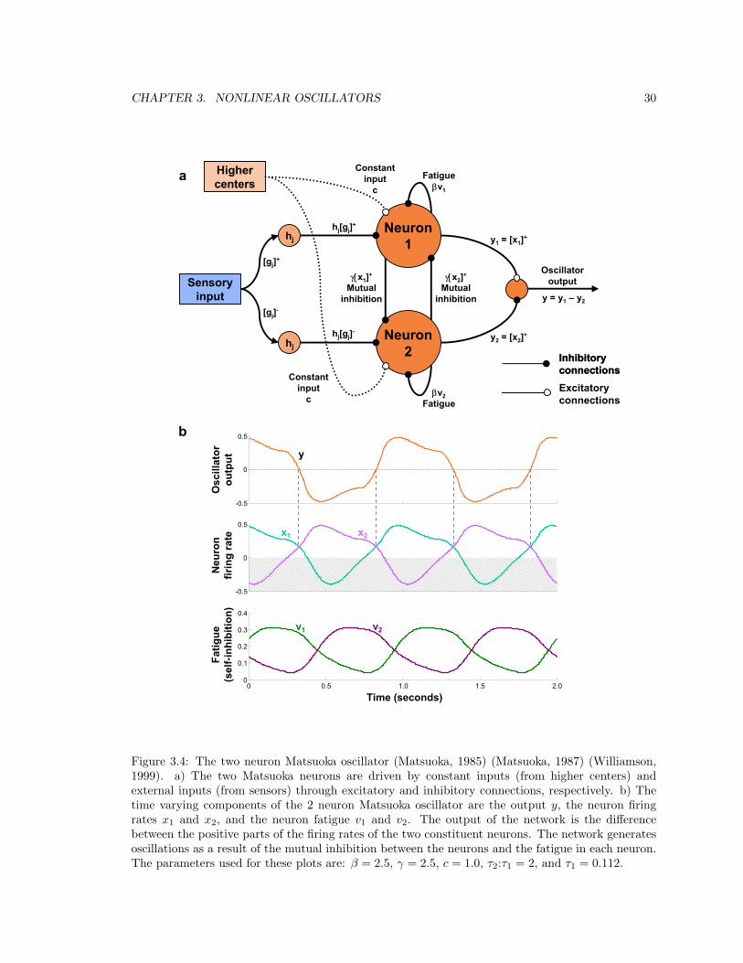
CHAPTER 3. NONLINEAR OSCILLATORS 30
Crop special 2.2
Usual crop is top and bottom: 2.3375Left and right: 1.4375
Neuron1
Neuron2
hj
hj
Sensoryinput
InhibitoryconnectionsInhibitoryconnectionsExcitatoryconnections
Highercenters
y1 = [x1]+
y2 = [x2]+
y = y1 – y2
Fatigueβv1
βv2Fatigue
γ[x2]+
Mutualinhibition
γ[x1]+
Mutualinhibition
Constantinput
c
Constantinput
c
Oscillatoroutput
[gj]+
[gj]-
hj[gj]+
hj[gj]-
-0.5
0
0.5
-0.5
0
0.5
0 0.5 1.0 1.5 2.00
0.1
0.2
0.3
0.4
Osc
illat
orou
tput
Time (seconds)
Neu
ron
firin
g ra
teFa
tigue
(sel
f-inh
ibiti
on)
v1 v2
x1 x2
y
b
a
From 05_3
Figure 3.4: The two neuron Matsuoka oscillator (Matsuoka, 1985) (Matsuoka, 1987) (Williamson,1999). a) The two Matsuoka neurons are driven by constant inputs (from higher centers) andexternal inputs (from sensors) through excitatory and inhibitory connections, respectively. b) Thetime varying components of the 2 neuron Matsuoka oscillator are the output y, the neuron firingrates x1 and x2, and the neuron fatigue v1 and v2. The output of the network is the differencebetween the positive parts of the firing rates of the two constituent neurons. The network generatesoscillations as a result of the mutual inhibition between the neurons and the fatigue in each neuron.The parameters used for these plots are: β = 2.5, γ = 2.5, c = 1.0, τ2:τ1 = 2, and τ1 = 0.112.
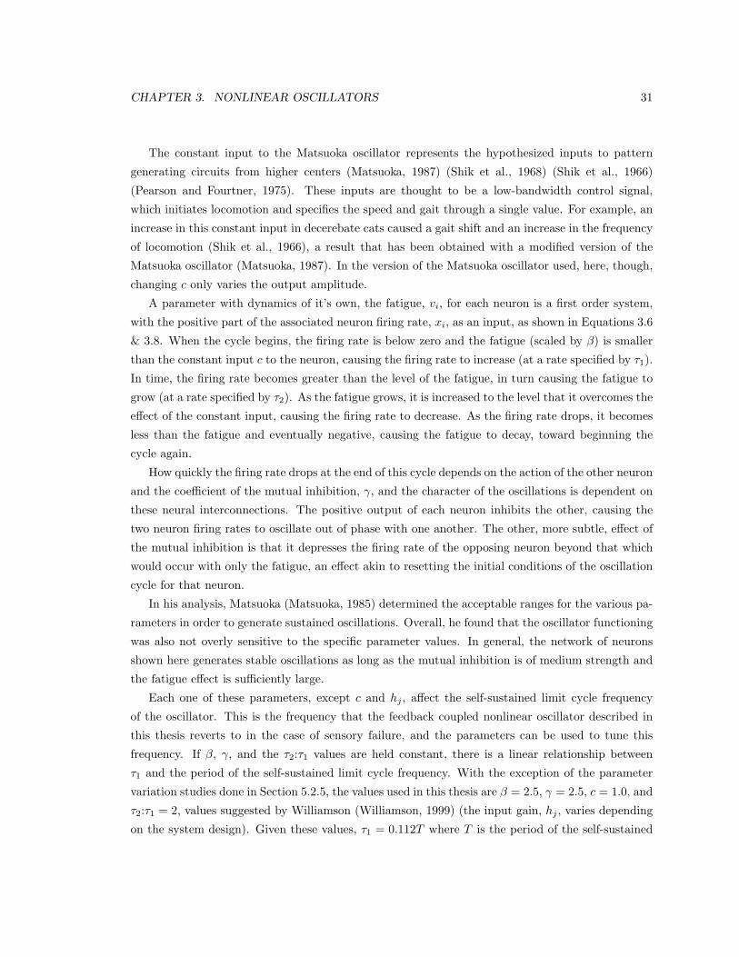
CHAPTER 3. NONLINEAR OSCILLATORS 31
The constant input to the Matsuoka oscillator represents the hypothesized inputs to pattern
generating circuits from higher centers (Matsuoka, 1987) (Shik et al., 1968) (Shik et al., 1966)
(Pearson and Fourtner, 1975). These inputs are thought to be a low-bandwidth control signal,
which initiates locomotion and specifies the speed and gait through a single value. For example, an
increase in this constant input in decerebate cats caused a gait shift and an increase in the frequency
of locomotion (Shik et al., 1966), a result that has been obtained with a modified version of the
Matsuoka oscillator (Matsuoka, 1987). In the version of the Matsuoka oscillator used, here, though,
changing c only varies the output amplitude.
A parameter with dynamics of it’s own, the fatigue, vi, for each neuron is a first order system,
with the positive part of the associated neuron firing rate, xi, as an input, as shown in Equations 3.6
& 3.8. When the cycle begins, the firing rate is below zero and the fatigue (scaled by β) is smaller
than the constant input c to the neuron, causing the firing rate to increase (at a rate specified by τ1).
In time, the firing rate becomes greater than the level of the fatigue, in turn causing the fatigue to
grow (at a rate specified by τ2). As the fatigue grows, it is increased to the level that it overcomes the
effect of the constant input, causing the firing rate to decrease. As the firing rate drops, it becomes
less than the fatigue and eventually negative, causing the fatigue to decay, toward beginning the
cycle again.
How quickly the firing rate drops at the end of this cycle depends on the action of the other neuron
and the coefficient of the mutual inhibition, γ, and the character of the oscillations is dependent on
these neural interconnections. The positive output of each neuron inhibits the other, causing the
two neuron firing rates to oscillate out of phase with one another. The other, more subtle, effect of
the mutual inhibition is that it depresses the firing rate of the opposing neuron beyond that which
would occur with only the fatigue, an effect akin to resetting the initial conditions of the oscillation
cycle for that neuron.
In his analysis, Matsuoka (Matsuoka, 1985) determined the acceptable ranges for the various pa-
rameters in order to generate sustained oscillations. Overall, he found that the oscillator functioning
was also not overly sensitive to the specific parameter values. In general, the network of neurons
shown here generates stable oscillations as long as the mutual inhibition is of medium strength and
the fatigue effect is sufficiently large.
Each one of these parameters, except c and hj , affect the self-sustained limit cycle frequency
of the oscillator. This is the frequency that the feedback coupled nonlinear oscillator described in
this thesis reverts to in the case of sensory failure, and the parameters can be used to tune this
frequency. If β, γ, and the τ2:τ1 values are held constant, there is a linear relationship between
τ1 and the period of the self-sustained limit cycle frequency. With the exception of the parameter
variation studies done in Section 5.2.5, the values used in this thesis are β = 2.5, γ = 2.5, c = 1.0, and
τ2:τ1 = 2, values suggested by Williamson (Williamson, 1999) (the input gain, hj , varies depending
on the system design). Given these values, τ1 = 0.112T where T is the period of the self-sustained

CHAPTER 3. NONLINEAR OSCILLATORS 32
oscillation.
Many other models have also been able to capture sustained oscillations through mutual inhibi-
tion and fatigue (Matsuoka, 1985), but these were either not general (Morishita and Yajima, 1972)
or the specific conditions necessary for oscillations were difficult to produce as a result of the digital
properties of the models (Reiss, 1962) (Kling and Szekely, 1968) (Suzuki et al., 1971) (Friesen and
Stent, 1977) (Nagashino et al., 1981).
In addition, the particular formulation of this oscillator allows it to have properties of so-called
“relaxation” nonlinear oscillators, such as an output amplitude independent of the input, but without
the associated numerical integration and stability issues. For example, the van der Pol oscillator
(Equation 3.1 with large ε values is a relaxation oscillator, and is a common example of a stiff
problem that is difficult to numerically integrate (Matlab Version 6.5 Release 13 Help Manual). In
contrast, numerical integration of the Matsuoka oscillator was found to be easy and stable, as the
only nonlinearities present are from the [xi]+, [gj ]+, and [gj ]− terms.
The following chapter explores feedback coupled oscillatory behavior during high speed animal
locomotion, modeling the pattern generators of the animal with a feedback coupled nonlinear oscilla-
tor. The fundamental characteristics of nonlinear oscillators discussed here, the self-sustained limit
cycle frequency and selective entrainment, are used to predict the behavior of the animal in response
to sustained cyclic perturbations and the experimental results show that the behavior observed is
consistent with a feedback coupled nonlinear oscillator model.
Later, in Chapter 5, design and analysis tools are developed for creating adaptive controllers
with feedback coupled nonlinear oscillators for cyclic dynamic tasks. In Chapter 6, the usefulness
of such a controller for legged robotic systems is demonstrated, with an emphasis on a visual design
procedure and the ability of the analysis tools to indicate the type of feedback needed to generate
the desired adaptive behavior.
Chapter 4
Biological inspiration: Sensory
influence on motor pattern
generators
It’s really criminal how little we know about the brain.
-Reza Shadmehr
In this chapter, the role of sensory information in determining the motor patterns the nervous
system generates for locomotion is examined. It is well accepted that general neural pattern gen-
erators are influenced by sensory information, but no work has been done on an intact, naturally
behaving running animal as is done here. The results of the experiments performed reveal that the
sensory information is used, even at the highest speeds of locomotion, and the behavior observed is
consistent with the feedback coupled nonlinear oscillator model of the nervous system.
This work is used as inspiration for the remainder of this thesis, which focuses on designing
feedback coupled nonlinear oscillators as adaptive controllers for legged robots, and cyclic dynamic
tasks in general. In turn, these subsequent chapters provide one possible explanation for the observed
results and generalize to provide a method for designing and tuning a system composed of a robot
or animal performing a cyclic dynamic task such as running, coupled to a nonlinear oscillator for
control.
This chapter begins by reviewing the previous work on animal pattern generators. Most of
these studies are on reduced specimens, ones that have been partially dissected and are operating
in unnatural environments. An exception to this trend is the work done by Wendler, who studied
locust flight (Wendler, 1974). Using a mostly intact animal in a relatively natural environment, he
analyzed the nervous system response by examining the relative phase between a cyclic mechanical
33
CHAPTER 4. BIOLOGICAL INSPIRATION 34
perturbation and the electromyogram (EMG) signal recorded from a muscle.
Representing the input and output of the nervous system, respectively, this method is adopted
for the work that is presented here. For these experiments, a running cockroach is allowed to run
freely on an inertial spherical treadmill, and is subjected to cyclic mechanical perturbations as the
EMG signals to one muscle are recorded. These experiments demonstrate that:
1. Motor pattern generators are influenced by sensory information, even at the highest speeds of
locomotion
2. The responses observed are consistent with a feedback coupled nonlinear oscillator model of
the motor pattern generators
Directional statistics techniques are used to quantify the results of the experiments, and are compared
to control cases without cyclic perturbations.
This chapter concludes with a discussion of the results of the experiments. Not all animals
exhibited behavior consistent with feedback coupled nonlinear oscillators, and possible reasons for
these anomalies are discussed.
4.1 Previous work on pattern generators
Motor pattern generation has been a rich field of research since Sherrington’s early work on sponta-
neous limb movements (Sherrington, 1906). Brown (Graham-Brown, 1922) hypothesized how these
cyclic movements could be generated by components in the nervous system, but evidence for motor
pattern generation from an isolated component of the nervous was not shown until the late 1970’s
(Grillner and Zangger, 1979), proving the existence of central pattern generators.
4.1.1 Central pattern generators
The terms pattern generators and central pattern generators are often used interchangeably, but
this thesis uses the terminology as defined by Bassler (Bassler, 1986). Pattern generators (PGs)
refers to all the neural circuits in a complete animal that are responsible for the generation of motor
commands, including sensory feedback circuits. Central pattern generators (CPGs), on the other
hand, refer to only one part of the system, the portion that is capable of generating motor patterns
in isolation.
Grillner’s work established that portions of the nervous system could generate motor patterns
for cyclic motor tasks without any sensory information (Grillner and Zangger, 1979). Further, these
motor patterns are not simply alternating bursts of activity - they appear to be specific enough to
compose the detailed phase relationships necessary for multi-joint locomotion (Grillner and Zangger,
1975). Grillner’s work involved partially dissected cats and lamprey (Cohen and Wallen, 1980), but
CHAPTER 4. BIOLOGICAL INSPIRATION 35
was replicated in other similarly reduced animals as well, including vertebrates and invertebrates
(Abbas and Full, 2000).
4.1.2 Sensory modulation
More recently, research on these circuits has turned toward their sensory modulation. In natu-
rally behaving intact animals, the central pattern generators and other components of the pattern
generators have access to sensory information as the animal performs cyclic motor tasks. Instead
of isolating the nervous system from input, these new experiments specifically provided artificial
sensory information to elicit responses from the pattern generators.
Much like the nonlinear oscillators discussed in the previous chapter, these circuits are capable of
generating their own rhythms but can be entrained by external stimuli (Guan et al., 2001) (Kiemel
and Cohen, 2001) (Andersson and Grillner, 1983). Additionally, it has been hypothesized that these
circuits are responsible for adaptive behaviors, such as the bending frequency modulation in response
to changes in water currents during lamprey swimming (Cohen and Boothe, 1999). This sensory
modulation has been shown in other animals as well, but the actual interaction mechanism is less
well understood.
The methods used to perform these experiments are varied, but often involve some partial dissec-
tion or deafferentation of the animal. These procedures often have damaging effects on the animal,
with unknown consequences for the results. More often, the animal is subjected to unnatural con-
ditions, and it is generally accepted that this can result in misleading interpretations of nervous
system function. Of course, there are exceptions to these generalities and one that is particularly
relevant to this thesis is Wendler’s work on locust flight regulation (Wendler, 1974).
4.1.3 Wendler’s experiments
The experiments in this chapter are largely inspired by the work that Wendler did on locusts,
especially with regard to the experimental methodology (Wendler, 1974). He provided the nervous
system with an sustained oscillatory input and measured the output, looking for a relationship
between the two by examining the phase difference between these two signals. The “preferred”
phase relationship he observed was consistent with the general nonlinear oscillator model of the
locust pattern generators.
One of the significant differences between this and other experiments is that the animal was
minimally damaged and the animal was allowed to move somewhat naturally. Of course, the animal
was operated on and tethered, but it was neither decapitated nor deafferented, and the unperturbed
wings were allowed to move freely. The behavioral differences are apparent when compared to studies
involving decapitation and deafferentation (Wilson and Wyman, 1965), as the responses to inputs
are fundamentally different in character.
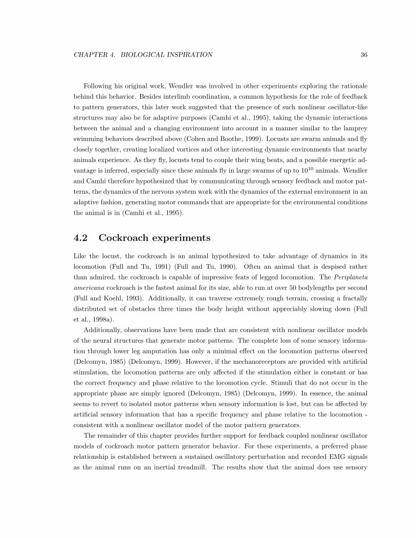
CHAPTER 4. BIOLOGICAL INSPIRATION 36
Following his original work, Wendler was involved in other experiments exploring the rationale
behind this behavior. Besides interlimb coordination, a common hypothesis for the role of feedback
to pattern generators, this later work suggested that the presence of such nonlinear oscillator-like
structures may also be for adaptive purposes (Camhi et al., 1995), taking the dynamic interactions
between the animal and a changing environment into account in a manner similar to the lamprey
swimming behaviors described above (Cohen and Boothe, 1999). Locusts are swarm animals and fly
closely together, creating localized vortices and other interesting dynamic environments that nearby
animals experience. As they fly, locusts tend to couple their wing beats, and a possible energetic ad-
vantage is inferred, especially since these animals fly in large swarms of up to 1010 animals. Wendler
and Camhi therefore hypothesized that by communicating through sensory feedback and motor pat-
terns, the dynamics of the nervous system work with the dynamics of the external environment in an
adaptive fashion, generating motor commands that are appropriate for the environmental conditions
the animal is in (Camhi et al., 1995).
4.2 Cockroach experiments
Like the locust, the cockroach is an animal hypothesized to take advantage of dynamics in its
locomotion (Full and Tu, 1991) (Full and Tu, 1990). Often an animal that is despised rather
than admired, the cockroach is capable of impressive feats of legged locomotion. The Periplaneta
americana cockroach is the fastest animal for its size, able to run at over 50 bodylengths per second
(Full and Koehl, 1993). Additionally, it can traverse extremely rough terrain, crossing a fractally
distributed set of obstacles three times the body height without appreciably slowing down (Full
et al., 1998a).
Additionally, observations have been made that are consistent with nonlinear oscillator models
of the neural structures that generate motor patterns. The complete loss of some sensory informa-
tion through lower leg amputation has only a minimal effect on the locomotion patterns observed
(Delcomyn, 1985) (Delcomyn, 1999). However, if the mechanoreceptors are provided with artificial
stimulation, the locomotion patterns are only affected if the stimulation either is constant or has
the correct frequency and phase relative to the locomotion cycle. Stimuli that do not occur in the
appropriate phase are simply ignored (Delcomyn, 1985) (Delcomyn, 1999). In essence, the animal
seems to revert to isolated motor patterns when sensory information is lost, but can be affected by
artificial sensory information that has a specific frequency and phase relative to the locomotion -
consistent with a nonlinear oscillator model of the motor pattern generators.
The remainder of this chapter provides further support for feedback coupled nonlinear oscillator
models of cockroach motor pattern generator behavior. For these experiments, a preferred phase
relationship is established between a sustained oscillatory perturbation and recorded EMG signals
as the animal runs on an inertial treadmill. The results show that the animal does use sensory
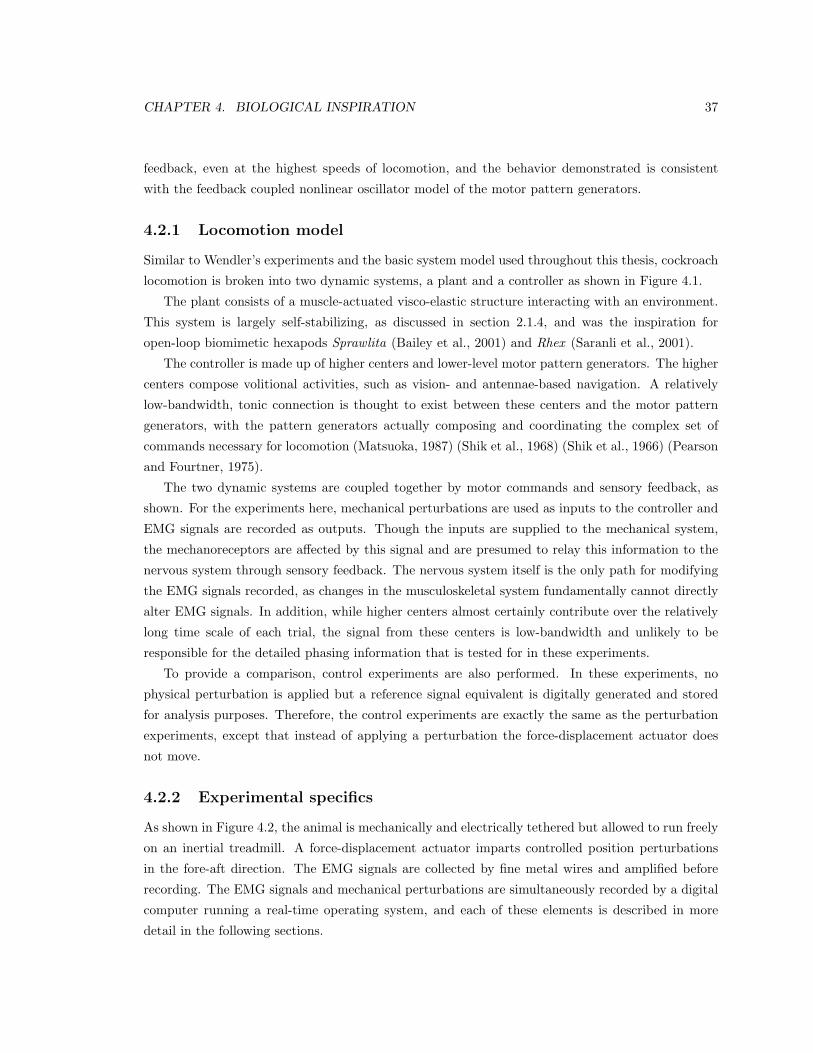
CHAPTER 4. BIOLOGICAL INSPIRATION 37
feedback, even at the highest speeds of locomotion, and the behavior demonstrated is consistent
with the feedback coupled nonlinear oscillator model of the motor pattern generators.
4.2.1 Locomotion model
Similar to Wendler’s experiments and the basic system model used throughout this thesis, cockroach
locomotion is broken into two dynamic systems, a plant and a controller as shown in Figure 4.1.
The plant consists of a muscle-actuated visco-elastic structure interacting with an environment.
This system is largely self-stabilizing, as discussed in section 2.1.4, and was the inspiration for
open-loop biomimetic hexapods Sprawlita (Bailey et al., 2001) and Rhex (Saranli et al., 2001).
The controller is made up of higher centers and lower-level motor pattern generators. The higher
centers compose volitional activities, such as vision- and antennae-based navigation. A relatively
low-bandwidth, tonic connection is thought to exist between these centers and the motor pattern
generators, with the pattern generators actually composing and coordinating the complex set of
commands necessary for locomotion (Matsuoka, 1987) (Shik et al., 1968) (Shik et al., 1966) (Pearson
and Fourtner, 1975).
The two dynamic systems are coupled together by motor commands and sensory feedback, as
shown. For the experiments here, mechanical perturbations are used as inputs to the controller and
EMG signals are recorded as outputs. Though the inputs are supplied to the mechanical system,
the mechanoreceptors are affected by this signal and are presumed to relay this information to the
nervous system through sensory feedback. The nervous system itself is the only path for modifying
the EMG signals recorded, as changes in the musculoskeletal system fundamentally cannot directly
alter EMG signals. In addition, while higher centers almost certainly contribute over the relatively
long time scale of each trial, the signal from these centers is low-bandwidth and unlikely to be
responsible for the detailed phasing information that is tested for in these experiments.
To provide a comparison, control experiments are also performed. In these experiments, no
physical perturbation is applied but a reference signal equivalent is digitally generated and stored
for analysis purposes. Therefore, the control experiments are exactly the same as the perturbation
experiments, except that instead of applying a perturbation the force-displacement actuator does
not move.
4.2.2 Experimental specifics
As shown in Figure 4.2, the animal is mechanically and electrically tethered but allowed to run freely
on an inertial treadmill. A force-displacement actuator imparts controlled position perturbations
in the fore-aft direction. The EMG signals are collected by fine metal wires and amplified before
recording. The EMG signals and mechanical perturbations are simultaneously recorded by a digital
computer running a real-time operating system, and each of these elements is described in more
detail in the following sections.
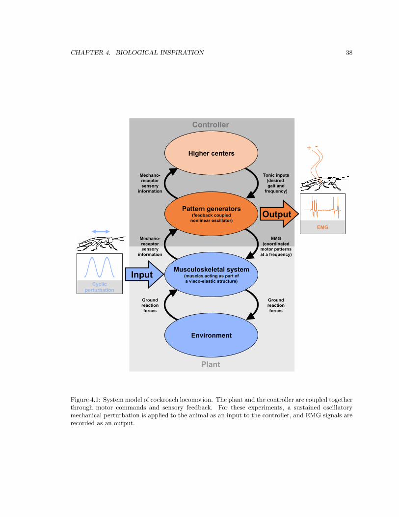
CHAPTER 4. BIOLOGICAL INSPIRATION 38
Mechano-receptorsensory
information
EMG(coordinated
motor patternsat a frequency)
Tonic inputs(desired gait and
frequency)
Groundreactionforces
Mechano-receptorsensory
information
Groundreactionforces
Higher centers
Environment
Pattern generators(feedback coupled
nonlinear oscillator)
Musculoskeletal system(muscles acting as part ofa visco-elastic structure)
InputCyclic
perturbation
OutputEMG
Plant
Controller
+ -
Figure 4.1: System model of cockroach locomotion. The plant and the controller are coupled togetherthrough motor commands and sensory feedback. For these experiments, a sustained oscillatorymechanical perturbation is applied to the animal as an input to the controller, and EMG signals arerecorded as an output.
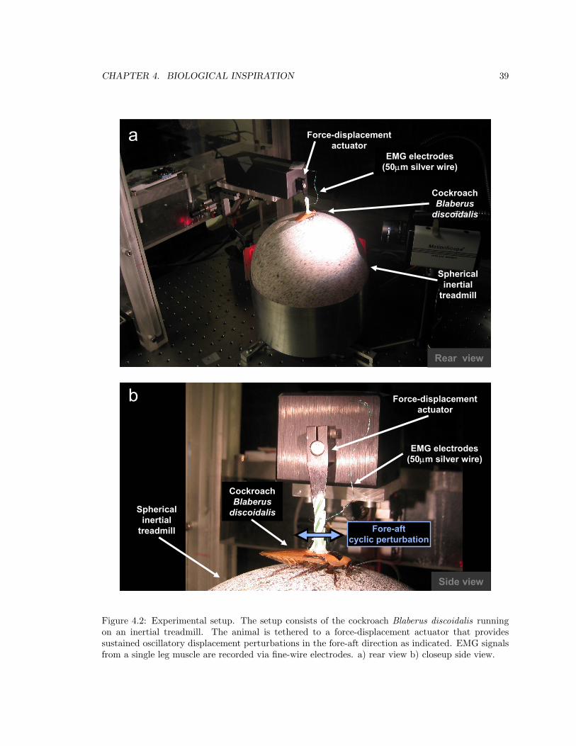
CHAPTER 4. BIOLOGICAL INSPIRATION 39
aEMG electrodes
(50µm silver wire)
Force-displacementactuator
CockroachBlaberusdiscoidalis
Sphericalinertial
treadmill
Rear view
b Force-displacementactuator
CockroachBlaberusdiscoidalisSpherical
inertialtreadmill
EMG electrodes(50µm silver wire)
Fore-aftcyclic perturbation
Side view
Figure 4.2: Experimental setup. The setup consists of the cockroach Blaberus discoidalis runningon an inertial treadmill. The animal is tethered to a force-displacement actuator that providessustained oscillatory displacement perturbations in the fore-aft direction as indicated. EMG signalsfrom a single leg muscle are recorded via fine-wire electrodes. a) rear view b) closeup side view.
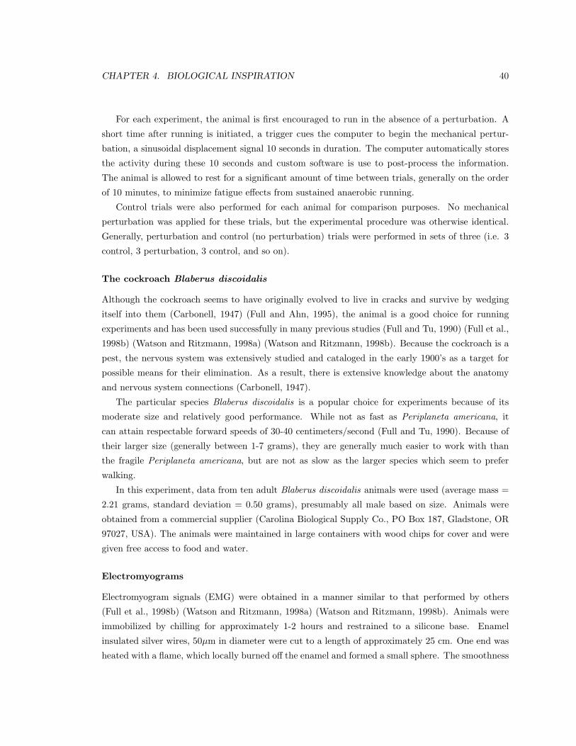
CHAPTER 4. BIOLOGICAL INSPIRATION 40
For each experiment, the animal is first encouraged to run in the absence of a perturbation. A
short time after running is initiated, a trigger cues the computer to begin the mechanical pertur-
bation, a sinusoidal displacement signal 10 seconds in duration. The computer automatically stores
the activity during these 10 seconds and custom software is use to post-process the information.
The animal is allowed to rest for a significant amount of time between trials, generally on the order
of 10 minutes, to minimize fatigue effects from sustained anaerobic running.
Control trials were also performed for each animal for comparison purposes. No mechanical
perturbation was applied for these trials, but the experimental procedure was otherwise identical.
Generally, perturbation and control (no perturbation) trials were performed in sets of three (i.e. 3
control, 3 perturbation, 3 control, and so on).
The cockroach Blaberus discoidalis
Although the cockroach seems to have originally evolved to live in cracks and survive by wedging
itself into them (Carbonell, 1947) (Full and Ahn, 1995), the animal is a good choice for running
experiments and has been used successfully in many previous studies (Full and Tu, 1990) (Full et al.,
1998b) (Watson and Ritzmann, 1998a) (Watson and Ritzmann, 1998b). Because the cockroach is a
pest, the nervous system was extensively studied and cataloged in the early 1900’s as a target for
possible means for their elimination. As a result, there is extensive knowledge about the anatomy
and nervous system connections (Carbonell, 1947).
The particular species Blaberus discoidalis is a popular choice for experiments because of its
moderate size and relatively good performance. While not as fast as Periplaneta americana, it
can attain respectable forward speeds of 30-40 centimeters/second (Full and Tu, 1990). Because of
their larger size (generally between 1-7 grams), they are generally much easier to work with than
the fragile Periplaneta americana, but are not as slow as the larger species which seem to prefer
walking.
In this experiment, data from ten adult Blaberus discoidalis animals were used (average mass =
2.21 grams, standard deviation = 0.50 grams), presumably all male based on size. Animals were
obtained from a commercial supplier (Carolina Biological Supply Co., PO Box 187, Gladstone, OR
97027, USA). The animals were maintained in large containers with wood chips for cover and were
given free access to food and water.
Electromyograms
Electromyogram signals (EMG) were obtained in a manner similar to that performed by others
(Full et al., 1998b) (Watson and Ritzmann, 1998a) (Watson and Ritzmann, 1998b). Animals were
immobilized by chilling for approximately 1-2 hours and restrained to a silicone base. Enamel
insulated silver wires, 50µm in diameter were cut to a length of approximately 25 cm. One end was
heated with a flame, which locally burned off the enamel and formed a small sphere. The smoothness
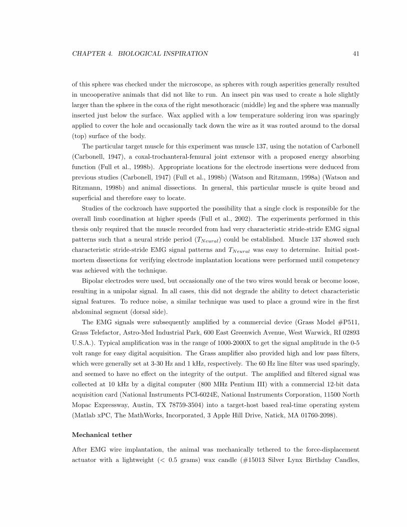
CHAPTER 4. BIOLOGICAL INSPIRATION 41
of this sphere was checked under the microscope, as spheres with rough asperities generally resulted
in uncooperative animals that did not like to run. An insect pin was used to create a hole slightly
larger than the sphere in the coxa of the right mesothoracic (middle) leg and the sphere was manually
inserted just below the surface. Wax applied with a low temperature soldering iron was sparingly
applied to cover the hole and occasionally tack down the wire as it was routed around to the dorsal
(top) surface of the body.
The particular target muscle for this experiment was muscle 137, using the notation of Carbonell
(Carbonell, 1947), a coxal-trochanteral-femural joint extensor with a proposed energy absorbing
function (Full et al., 1998b). Appropriate locations for the electrode insertions were deduced from
previous studies (Carbonell, 1947) (Full et al., 1998b) (Watson and Ritzmann, 1998a) (Watson and
Ritzmann, 1998b) and animal dissections. In general, this particular muscle is quite broad and
superficial and therefore easy to locate.
Studies of the cockroach have supported the possibility that a single clock is responsible for the
overall limb coordination at higher speeds (Full et al., 2002). The experiments performed in this
thesis only required that the muscle recorded from had very characteristic stride-stride EMG signal
patterns such that a neural stride period (TNeural) could be established. Muscle 137 showed such
characteristic stride-stride EMG signal patterns and TNeural was easy to determine. Initial post-
mortem dissections for verifying electrode implantation locations were performed until competency
was achieved with the technique.
Bipolar electrodes were used, but occasionally one of the two wires would break or become loose,
resulting in a unipolar signal. In all cases, this did not degrade the ability to detect characteristic
signal features. To reduce noise, a similar technique was used to place a ground wire in the first
abdominal segment (dorsal side).
The EMG signals were subsequently amplified by a commercial device (Grass Model #P511,
Grass Telefactor, Astro-Med Industrial Park, 600 East Greenwich Avenue, West Warwick, RI 02893
U.S.A.). Typical amplification was in the range of 1000-2000X to get the signal amplitude in the 0-5
volt range for easy digital acquisition. The Grass amplifier also provided high and low pass filters,
which were generally set at 3-30 Hz and 1 kHz, respectively. The 60 Hz line filter was used sparingly,
and seemed to have no effect on the integrity of the output. The amplified and filtered signal was
collected at 10 kHz by a digital computer (800 MHz Pentium III) with a commercial 12-bit data
acquisition card (National Instruments PCI-6024E, National Instruments Corporation, 11500 North
Mopac Expressway, Austin, TX 78759-3504) into a target-host based real-time operating system
(Matlab xPC, The MathWorks, Incorporated, 3 Apple Hill Drive, Natick, MA 01760-2098).
Mechanical tether
After EMG wire implantation, the animal was mechanically tethered to the force-displacement
actuator with a lightweight (< 0.5 grams) wax candle (#15013 Silver Lynx Birthday Candles,

CHAPTER 4. BIOLOGICAL INSPIRATION 42
Navajo Manufacturing Company, Incorporated, 5330 Fox Street, Denver, CO 80216), as shown in
Figure 4.2. The candle was attached to the relatively stiff dorsal thorax (back of the animal) using
cyanoacrylate ester (Partsmaster Gapper, Partsmaster, P.O. Box 655326, Dallas, TX 75265-5326).
Only a small part of the wing structure was removed, taking care to minimize damage to the animal.
The other end of the candle was simply melted onto the arm of the force-displacement actuator.
Inertial treadmill
An inertial treadmill is a regular treadmill in the sense that the runner stays in place as the treadmill
turns. However, regular treadmills have specified velocities and create a special Newtonian reference
frame, regardless of the forces imparted on them by the runners. While this apparatus works well
for runners that are not mechanically tethered, it is inappropriate to both tether the animal and
use a regular treadmill. If the runner is mechanically tethered, an inertial treadmill is needed - one
whose inertia matches the inertia of the animal as it accelerates and decelerates with each stride.
The inertial treadmill used in this experiment is similar in design to the ones introduced by
Kramer and Okada (Kramer, 1976) (Okada and Toh, 2000). The particular inertial treadmill used
in this experiment is a 0.2 meter diameter thin (approximately 0.67 millimeter) spherical shell
of expanded polystyrene, one of the lightest manufactured materials with a density of about 20
kilograms/meter3. This hollow sphere is supported by an air bearing, as shown in Figure 4.2,
operating at a pressure of 0.05 pounds/inch2. The air bearing allows the sphere to rotate freely and
with very little friction.
As the animal is mechanically tethered to the force-displacement actuator, the rotational inertia
of the sphere is used as a substitute for the animal body inertia. The particular mass distribution
of this particular inertial treadmill is tuned for a 4.5 gram animal, as an animal of this size would
experience the same fore-aft ground reaction forces as it would if it were running on solid ground.
The animal therefore runs naturally and experiences dynamics similar to those it would normally
feel during running on stationary ground.
The use of an inertial treadmill also has other advantages that are crucial for this experiment.
First, the animal stays in one place during the entire experiment. This allows the animal to be
tethered to the force-displacement actuator for perturbations, eliminating the need for more extreme
methods such as miniature cannons glued to the animal’s back (Jindrich, 2001) (Barry, 2002). While
used in this experiment only to help develop the technique and verify a one-to-one correlation between
EMG and musculoskeletal kinematics, it is easy to capture long lengths of high speed video as the
animal stays in one place regardless of running speed. In addition, EMG wire management is
made easy, as entanglements never occur (a common problem with long leads in open arenas). The
length of the EMG wire could also be kept short, which reduces the noise and unintended dynamic
interactions possible with a long tether.
There are many potential sources of error with this configuration, which should be noted here.
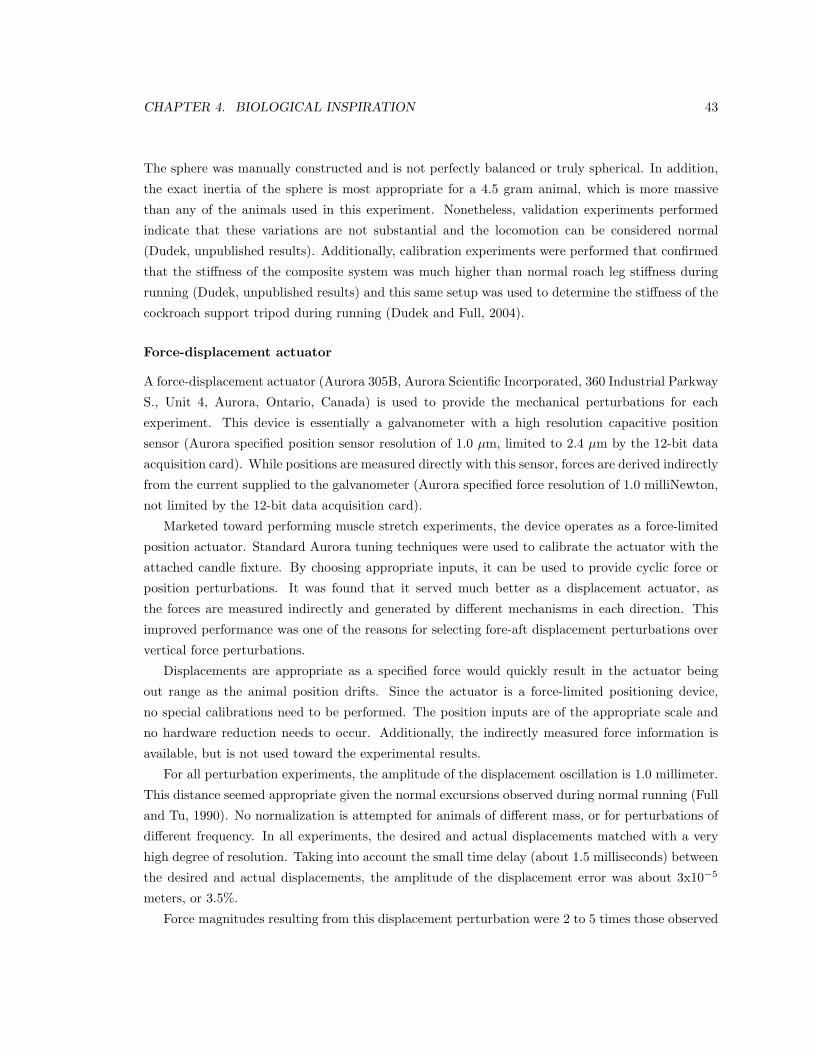
CHAPTER 4. BIOLOGICAL INSPIRATION 43
The sphere was manually constructed and is not perfectly balanced or truly spherical. In addition,
the exact inertia of the sphere is most appropriate for a 4.5 gram animal, which is more massive
than any of the animals used in this experiment. Nonetheless, validation experiments performed
indicate that these variations are not substantial and the locomotion can be considered normal
(Dudek, unpublished results). Additionally, calibration experiments were performed that confirmed
that the stiffness of the composite system was much higher than normal roach leg stiffness during
running (Dudek, unpublished results) and this same setup was used to determine the stiffness of the
cockroach support tripod during running (Dudek and Full, 2004).
Force-displacement actuator
A force-displacement actuator (Aurora 305B, Aurora Scientific Incorporated, 360 Industrial Parkway
S., Unit 4, Aurora, Ontario, Canada) is used to provide the mechanical perturbations for each
experiment. This device is essentially a galvanometer with a high resolution capacitive position
sensor (Aurora specified position sensor resolution of 1.0 µm, limited to 2.4 µm by the 12-bit data
acquisition card). While positions are measured directly with this sensor, forces are derived indirectly
from the current supplied to the galvanometer (Aurora specified force resolution of 1.0 milliNewton,
not limited by the 12-bit data acquisition card).
Marketed toward performing muscle stretch experiments, the device operates as a force-limited
position actuator. Standard Aurora tuning techniques were used to calibrate the actuator with the
attached candle fixture. By choosing appropriate inputs, it can be used to provide cyclic force or
position perturbations. It was found that it served much better as a displacement actuator, as
the forces are measured indirectly and generated by different mechanisms in each direction. This
improved performance was one of the reasons for selecting fore-aft displacement perturbations over
vertical force perturbations.
Displacements are appropriate as a specified force would quickly result in the actuator being
out range as the animal position drifts. Since the actuator is a force-limited positioning device,
no special calibrations need to be performed. The position inputs are of the appropriate scale and
no hardware reduction needs to occur. Additionally, the indirectly measured force information is
available, but is not used toward the experimental results.
For all perturbation experiments, the amplitude of the displacement oscillation is 1.0 millimeter.
This distance seemed appropriate given the normal excursions observed during normal running (Full
and Tu, 1990). No normalization is attempted for animals of different mass, or for perturbations of
different frequency. In all experiments, the desired and actual displacements matched with a very
high degree of resolution. Taking into account the small time delay (about 1.5 milliseconds) between
the desired and actual displacements, the amplitude of the displacement error was about 3x10⁻⁵
meters, or 3.5%.
Force magnitudes resulting from this displacement perturbation were 2 to 5 times those observed
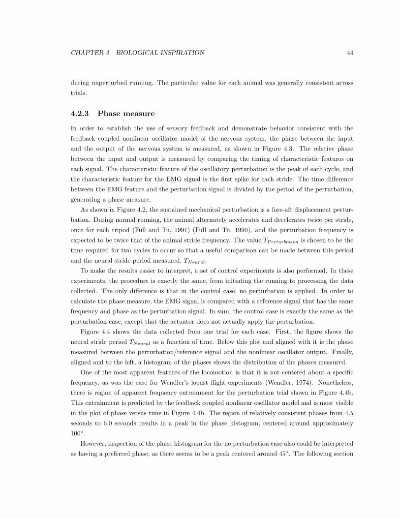
CHAPTER 4. BIOLOGICAL INSPIRATION 44
during unperturbed running. The particular value for each animal was generally consistent across
trials.
4.2.3 Phase measure
In order to establish the use of sensory feedback and demonstrate behavior consistent with the
feedback coupled nonlinear oscillator model of the nervous system, the phase between the input
and the output of the nervous system is measured, as shown in Figure 4.3. The relative phase
between the input and output is measured by comparing the timing of characteristic features on
each signal. The characteristic feature of the oscillatory perturbation is the peak of each cycle, and
the characteristic feature for the EMG signal is the first spike for each stride. The time difference
between the EMG feature and the perturbation signal is divided by the period of the perturbation,
generating a phase measure.
As shown in Figure 4.2, the sustained mechanical perturbation is a fore-aft displacement pertur-
bation. During normal running, the animal alternately accelerates and decelerates twice per stride,
once for each tripod (Full and Tu, 1991) (Full and Tu, 1990), and the perturbation frequency is
expected to be twice that of the animal stride frequency. The value TPerturbation is chosen to be the
time required for two cycles to occur so that a useful comparison can be made between this period
and the neural stride period measured, TNeural.
To make the results easier to interpret, a set of control experiments is also performed. In these
experiments, the procedure is exactly the same, from initiating the running to processing the data
collected. The only difference is that in the control case, no perturbation is applied. In order to
calculate the phase measure, the EMG signal is compared with a reference signal that has the same
frequency and phase as the perturbation signal. In sum, the control case is exactly the same as the
perturbation case, except that the actuator does not actually apply the perturbation.
Figure 4.4 shows the data collected from one trial for each case. First, the figure shows the
neural stride period TNeural as a function of time. Below this plot and aligned with it is the phase
measured between the perturbation/reference signal and the nonlinear oscillator output. Finally,
aligned and to the left, a histogram of the phases shows the distribution of the phases measured.
One of the most apparent features of the locomotion is that it is not centered about a specific
frequency, as was the case for Wendler’s locust flight experiments (Wendler, 1974). Nonetheless,
there is region of apparent frequency entrainment for the perturbation trial shown in Figure 4.4b.
This entrainment is predicted by the feedback coupled nonlinear oscillator model and is most visible
in the plot of phase versus time in Figure 4.4b. The region of relatively consistent phases from 4.5
seconds to 6.0 seconds results in a peak in the phase histogram, centered around approximately
100◦.
However, inspection of the phase histogram for the no perturbation case also could be interpreted
as having a preferred phase, as there seems to be a peak centered around 45◦. The following section
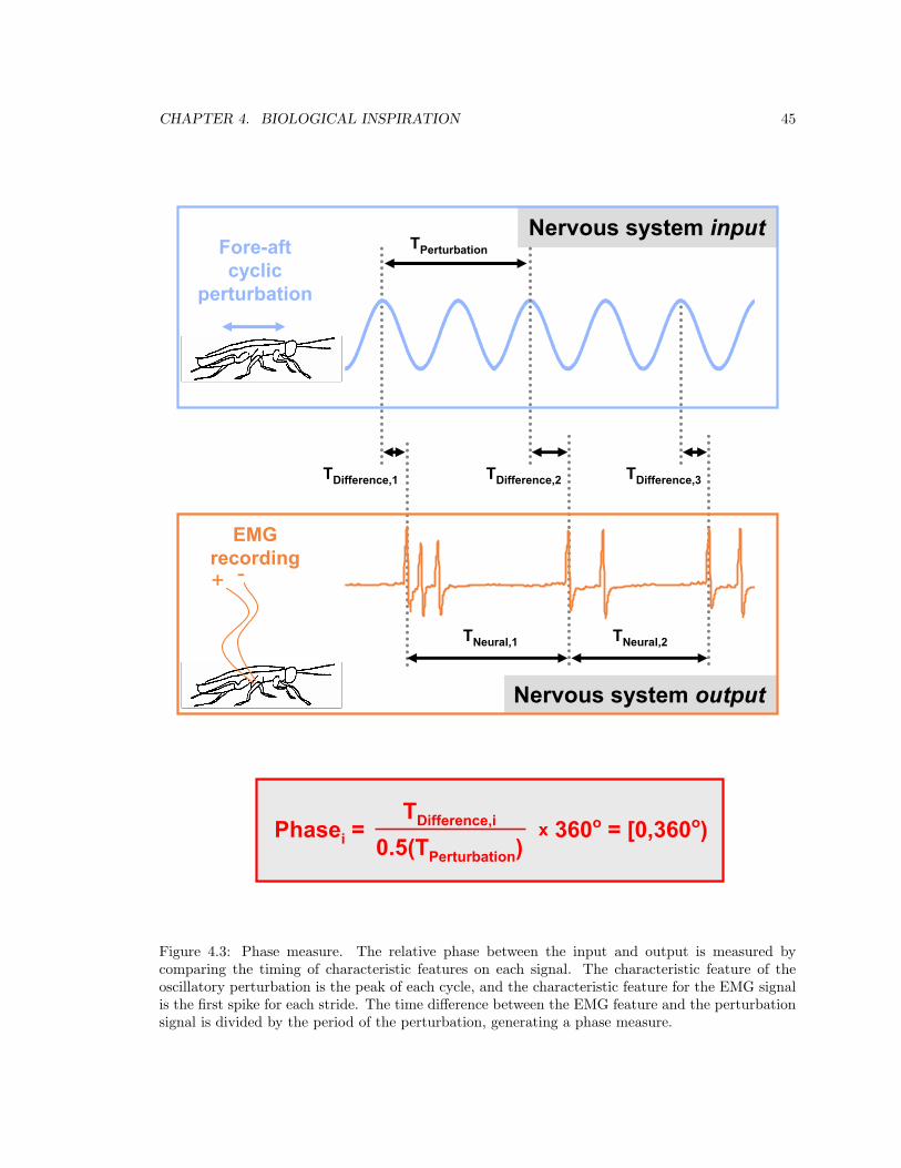
CHAPTER 4. BIOLOGICAL INSPIRATION 45
Nervous system inputFore-aftcyclic
perturbation
EMGrecording+ -
TPerturbation
TNeural,1
TDifference,1 TDifference,2 TDifference,3
TNeural,2
Nervous system output
Phasei =TDifference,i
0.5(TPerturbation)x 360o = [0,360o)
Figure 4.3: Phase measure. The relative phase between the input and output is measured bycomparing the timing of characteristic features on each signal. The characteristic feature of theoscillatory perturbation is the peak of each cycle, and the characteristic feature for the EMG signalis the first spike for each stride. The time difference between the EMG feature and the perturbationsignal is divided by the period of the perturbation, generating a phase measure.
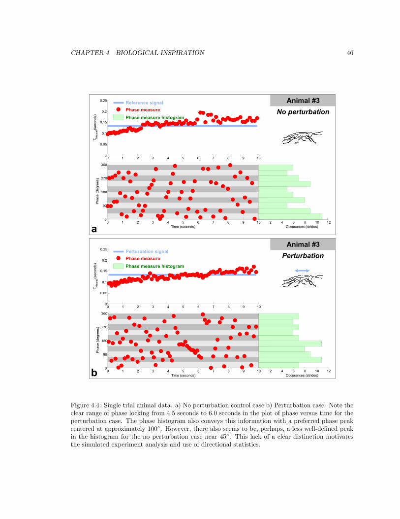
CHAPTER 4. BIOLOGICAL INSPIRATION 46
0 1 2 3 4 5 6 7 8 9 100
0.05
0.1
0.15
0.2
0.25
T Neu
ral(s
econ
ds)
0 1 2 3 4 5 6 7 8 9 100
90
180
270
360
Time (seconds)
Pha
se (d
egre
es)
2 4 6 8 10 12Occurances (strides)
0 1 2 3 4 5 6 7 8 9 100
0.05
0.1
0.15
0.2
0.25
T Neu
ral(s
econ
ds)
0 1 2 3 4 5 6 7 8 9 100
90
180
270
360
Time (seconds)
Pha
se (d
egre
es)
2 4 6 8 10 12Occurances (strides)
Experimental resultsNo perturbation
ExPe
ExpeNo p
Exppert
Animal #3No perturbation
Animal #3Perturbation
Reference signalPhase measurePhase measure histogram
Perturbation signalPhase measurePhase measure histogram
a
b
Figure 4.4: Single trial animal data. a) No perturbation control case b) Perturbation case. Note theclear range of phase locking from 4.5 seconds to 6.0 seconds in the plot of phase versus time for theperturbation case. The phase histogram also conveys this information with a preferred phase peakcentered at approximately 100◦. However, there also seems to be, perhaps, a less well-defined peakin the histogram for the no perturbation case near 45◦. This lack of a clear distinction motivatesthe simulated experiment analysis and use of directional statistics.
CHAPTER 4. BIOLOGICAL INSPIRATION 47
shows that this is an artifact of the non-centered stride frequency of the animal during the running,
and this effect is eliminated by looking at the data collected over multiple trials.
4.3 Simulated results
A preferred phase between the mechanical perturbation and the EMG signals indicates that the
sensory information generated by the perturbation is being used by the nervous system, and is
consistent with the feedback coupled nonlinear oscillator model of the motor pattern generators.
Unlike the locust experiments by Wendler (Wendler, 1974), the cockroach EMG signal frequency did
not center on a specific frequency for the duration of the experiment, making the phase measurement
results more difficult to interpret. Even though there is clearly a preferred phase for the perturbation
case shown in Figure 4.4, it is difficult to see if this is also the case for the control experiment, as
the histogram for that case has a peak as well, albeit more poorly defined.
Taking this into account, this section discusses in more detail the results that are predicted by the
feedback coupled nonlinear oscillator model. These expected results are generated by a numerical
simulation of a nonlinear oscillator driven by a sinusoidal forcing function. Directional statistics
techniques over multiple trials are then used to quantify the results comparing the perturbation and
control cases. Examining the data over multiple trials yields a preferred direction for the simulated
perturbation case and a uniform distribution for the control case, forming the approach used to
examine the actual data from the animal experiments performed.
4.3.1 The simulation model
The experiments described in this chapter test for general nonlinear oscillator characteristics in the
motor pattern generators. For the generation of expected results, however, the Matsuoka nonlinear
oscillator (Matsuoka, 1985) (Matsuoka, 1987) (Williamson, 1999) was chosen, as it was used in
Chapters 5 and 6 of this thesis. Described in more detail there and in Section 3.3.3, this oscillator is
based on neural principles. Additionally, the 2 neuron network with mutual inhibition has relaxation
properties but is easy to integrate (see Section 3.3.3).
In the animal experiments, the output of the nervous system is half the frequency of the me-
chanical perturbation. This is due to the fact that there are two steps (corresponding to the two
tripods) per stride, but the EMG signal is only collected from a single leg on one of the tripods.
Therefore, for each stride there are two displacement peaks but only one EMG pattern.
The simulated experiments are simplified, as the nonlinear oscillator model of the nervous system
and the mechanical perturbation are of the same frequency. To create a reference point analogous
to the first EMG spike of each stride for the animal, every other peak of the nonlinear oscillator
output is converted to an artificial spike. This spike is used to calculate TNeural and the relative
phase for each stride, using the same processing code as the animal experiments.
CHAPTER 4. BIOLOGICAL INSPIRATION 48
The perturbation case
To simulate the cyclic mechanical perturbation, a sinusoidal forcing function is applied to the os-
cillator. The perturbation is at a fixed frequency, and begins each trial at the same initial phase.
For this simulation, the forcing function frequency is fixed at 15.0 Hz, corresponding to a stride
frequency of 7.5 Hz. The amplitude of the forcing function signal is varied, ranging from 0.025 to
0.1. The specific values affected the strength of the entrainment and phase distributions observed,
but did not fundamentally change any of the expected results.
The control case
As with the animal experiments, control simulations are also performed. Instead of applying a
sinusoidal forcing function, the Matsuoka oscillator is allowed to run open-loop. The output signal
of the nonlinear oscillator is then compared to a 15.0 Hz reference signal that is a duplicate of the
forcing function used for the perturbation.
These two cases are shown in Figure 4.5. First, the figure shows the neural stride period TNeural
as a function of time. Below this plot and aligned with it is the phase measured between the
perturbation signal (or reference signal for the control case) and the nonlinear oscillator output.
Finally, aligned and to the left, a histogram of the phases shows the distribution of the phases
measured.
4.3.2 Simulation boundary conditions
Beginning and ending frequencies
As was shown in Figure 4.4, the neural stride period of the animal is not centered on a constant
value throughout the duration of the trial, a characteristic that is consistent in both the perturbation
and control cases. When the animal first begins to run, TNeural is relatively small, as the animal
is running at a high frequency. As the trial progresses, though, TNeural generally increases, as the
animal begins to slow down and run at a lower frequency. As TNeural changes, at some point during
the trial it crosses TPerturbation.
To replicate the effect of this drifting TNeural value in the simulation, the self-sustained limit
cycle period of the Matsuoka oscillator is varied during the course of the trial by changing τ1 (see
Section 5.2.5). As with the animal, the period is small at the beginning of the trial and becomes
larger as the trial progresses, going from a high frequency to a low frequency. At some point during
the trial, the TNeural value crosses the perturbation period as it lies in between the upper and lower
values and this effect is shown in Figure 4.5.
In addition, the beginning and ending periods of TNeural are varied randomly. The range of
beginning frequencies is 17-22 Hz, representing a stride frequency of 8.5-11 Hz. The ending periods
varied from 10-14 Hz, corresponding to a stride frequency range of 5-7 Hz. Both of these ranges
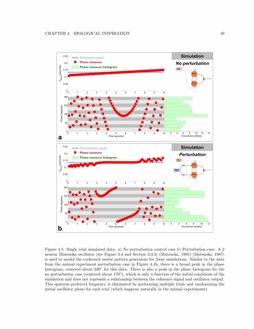
CHAPTER 4. BIOLOGICAL INSPIRATION 49
0 1 2 3 4 5 6 7 8 9 100
0.05
0.1
0.15
0.2
0.25T N
eura
l(sec
onds
)
0 1 2 3 4 5 6 7 8 9 100
90
180
270
360
Time (seconds)
Pha
se (d
egre
es)
2 4 6 8 10 12 14Occurances (strides)
Simulated resultsNo perturbation
0 1 2 3 4 5 6 7 8 9 100
0.05
0.1
0.15
0.2
0.25
T Neu
ral(s
econ
ds)
0 1 2 3 4 5 6 7 8 9 100
90
180
270
360
Time (seconds)
Pha
se (d
egre
es)
2 4 6 8 10 12Occurances (strides)
SimuPertu
Rando5015
Rando5004
SimulationNo perturbation
Reference signalPhase measurePhase measure histogram
Neuron1
Neuron2
Highercenters
Neuron1
Neuron2
Sensoryinput
Highercenters
SimulationPerturbation
Perturbation signalPhase measurePhase measure histogram
a
b
Figure 4.5: Single trial simulated data. a) No perturbation control case b) Perturbation case. A 2neuron Matsuoka oscillator (see Figure 3.4 and Section 3.3.3) (Matsuoka, 1985) (Matsuoka, 1987)is used to model the cockroach motor pattern generators for these simulations. Similar to the datafrom the animal experiment perturbation case in Figure 4.4b, there is a broad peak in the phasehistogram, centered about 330◦ for this data. There is also a peak in the phase histogram for theno perturbation case (centered about 170◦), which is only a function of the initial conditions of thesimulation and does not represent a relationship between the reference signal and oscillator output.This spurious preferred frequency is eliminated by performing multiple trials and randomizing theinitial oscillator phase for each trial (which happens naturally in the animal experiments).

CHAPTER 4. BIOLOGICAL INSPIRATION 50
correspond with the frequencies observed during the experiments, and with other studies on running
(Full and Tu, 1990). The ranges chosen did affect the resulting distributions, but for all cases, the
uniform and non-uniform characteristics discussed later were preserved.
Initial oscillator phase
The one boundary condition that is the most important for generating a useful prediction is the initial
phase of the Matsuoka oscillator. As was noticed with both the actual and simulated data in Figures
4.4 and 4.5, a non-uniform histogram indicates a preferred phase not only for the perturbation cases,
but also for the control cases where there was no perturbation.
On the surface this does not seem possible, as the animal cannot have any knowledge of the
reference signal and therefore cannot be selecting a preferred phase with it. Indeed, if the simulation
control case is initiated with the same Matsuoka initial conditions and frequency boundary conditions
each time, a preferred phase occurs at the same angle every time.
Closer examination reveals that this has nothing to do with entrainment, it is simply the rela-
tionship that occurs between two signals of this type. If a signal changes frequency from a high
value to a low value, and is compared with a signal with a frequency in between the two, then a
particular phase occurs more often than others, even if the two signals are completely independent.
This spurious preferred frequency occurs as a result of the chance phase relationship that exists at
the instant when the two signals have matching frequencies.
A simple case that illustrates this point is the example of fixing the nonlinear oscillator self-
sustained limit cycle frequency at the perturbation frequency, rather than varying it over a range.
As the two signals are of the same frequency, an initial phase relationship exists between the two
signals at the beginning of the trial. If the two signals are independent, the phase relationship
remains at this value. If the two signals are dependent, however, the phase relationship will shift
from this phase to the preferred phase between the two dependent signals.
If this is done over multiple trials and the initial phase is randomized, each individual trial
continues to exhibit a peak in the phase histogram, but it become trivial to distinguish between
independent and dependent signals. Independent trials maintain the initial, random phase relation-
ship while dependent signals instead converge to the preferred phase relationship. Therefore, when
multiple trials are examined, the distribution of histogram peaks from the independent signals is
random, or uniform, while the dependent signals are centered on one phase relationship, despite the
random initial conditions.
Thus, the simulations are seeded with pseudo-random phases and examined over multiple trials
to circumvent this effect. For the simulations presented here, the initial conditions are defined by
xRandom = Random(−0.5, 0.5), x1 = xRandom, x2 = −xRandom, and v1,2 = 0. It should be noted
that these initial conditions only approximate random phases of the oscillator, but the difference
does not appear to affect the results.
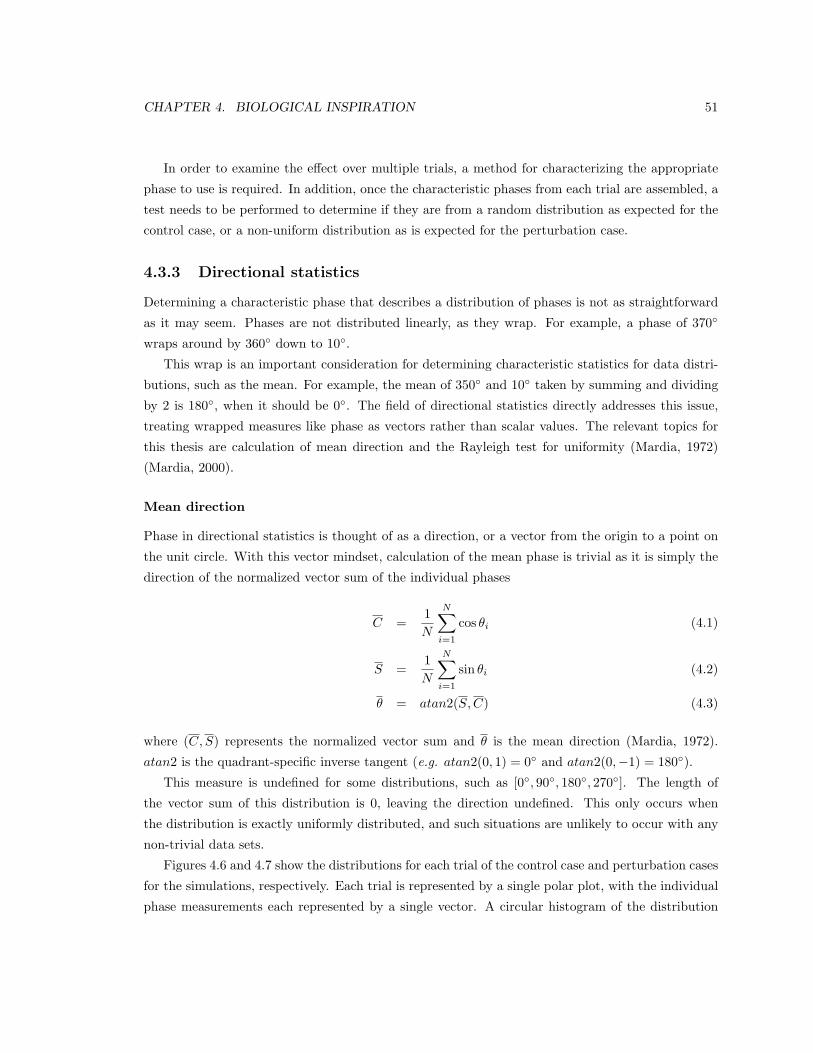
CHAPTER 4. BIOLOGICAL INSPIRATION 51
In order to examine the effect over multiple trials, a method for characterizing the appropriate
phase to use is required. In addition, once the characteristic phases from each trial are assembled, a
test needs to be performed to determine if they are from a random distribution as expected for the
control case, or a non-uniform distribution as is expected for the perturbation case.
4.3.3 Directional statistics
Determining a characteristic phase that describes a distribution of phases is not as straightforward
as it may seem. Phases are not distributed linearly, as they wrap. For example, a phase of 370◦
wraps around by 360◦ down to 10◦.
This wrap is an important consideration for determining characteristic statistics for data distri-
butions, such as the mean. For example, the mean of 350◦ and 10◦ taken by summing and dividing
by 2 is 180◦, when it should be 0◦. The field of directional statistics directly addresses this issue,
treating wrapped measures like phase as vectors rather than scalar values. The relevant topics for
this thesis are calculation of mean direction and the Rayleigh test for uniformity (Mardia, 1972)
(Mardia, 2000).
Mean direction
Phase in directional statistics is thought of as a direction, or a vector from the origin to a point on
the unit circle. With this vector mindset, calculation of the mean phase is trivial as it is simply the
direction of the normalized vector sum of the individual phases
C =1N
N∑i=1
cos θi (4.1)
S =1N
N∑i=1
sin θi (4.2)
θ = atan2(S,C) (4.3)
where (C, S) represents the normalized vector sum and θ is the mean direction (Mardia, 1972).
atan2 is the quadrant-specific inverse tangent (e.g. atan2(0, 1) = 0◦ and atan2(0,−1) = 180◦).
This measure is undefined for some distributions, such as [0◦, 90◦, 180◦, 270◦]. The length of
the vector sum of this distribution is 0, leaving the direction undefined. This only occurs when
the distribution is exactly uniformly distributed, and such situations are unlikely to occur with any
non-trivial data sets.
Figures 4.6 and 4.7 show the distributions for each trial of the control case and perturbation cases
for the simulations, respectively. Each trial is represented by a single polar plot, with the individual
phase measurements each represented by a single vector. A circular histogram of the distribution

CHAPTER 4. BIOLOGICAL INSPIRATION 52
for each trial is plotted in the background and the mean is represented by a single thick vector. The
summary plot shows the mean phase from each trial, with a circular histogram in the background.
Visual inspection of the summary distributions indicates that the trial means for the control case
are random and uniformly distributed, as would be expected for independent signals. The means
for the perturbation case are more focused and not uniform, as would be predicted for a feedback
coupled nonlinear oscillator. These simulated results validate this analysis method, but an additional
step needs to be taken to quantify the results.
The Rayleigh test
The Rayleigh test is a statistical method for quantifying the uniformity of directional data. In
particular, this test is appropriate when the underlying mean of the distribution is unknown, as is
the case here (Mardia, 1972).
The null hypothesis for this test is that the data are sampled from a uniform distribution. The
p-value returned represents the probability that rejecting this hypothesis is incorrect, and the level
of significance selected for these experiments is 0.05 (Devore and Farnum, 1999).
In other words, if the p-value returned by the test is larger than 0.05, then the null hypothesis
of uniformity is not rejected, and the data may or may not be from a uniform distribution. The
data may seem to be from a uniform distribution, but this test provides no statistical support for
this conclusion.
On the other hand, if the p-value is smaller than 0.05, then the null hypothesis is rejected and
it is statistically significant that the data are not from a uniform distribution. A p-value of 0.05
represents 95% certainty that the data are not from a uniform distribution, and is statistically
significant.
The procedure for the Rayleigh test is similar to that of the directional mean, except that the
length of the vector sum is of interest.
R2
= C2
+ S2
(4.4)
where R is the normalized vector sum, and C and S are from Equations 4.1 and 4.2, respectively.
Divided by the number of samples (in this case trials), this normalized length of the vector sum
indicates how directionally varied the data are. Intuitively, values close to 0 indicate uniformly
distributed data, while values close to 1 indicate that the data are quite focused. This value can
be corrected and compared to a chi-squared distribution with 2 degrees of freedom (χ22). For small
samples it is easier to refer to a chart of values to determine the p-value (Mardia, 1972). The
threshold value of R depends on N , where N is the number of trials performed.
The Rayleigh test confirms preliminary conclusions from the visual inspections of Figures 4.6
and 4.7. The summary plot for the no perturbation control case resulted in a R = 0.28. This value
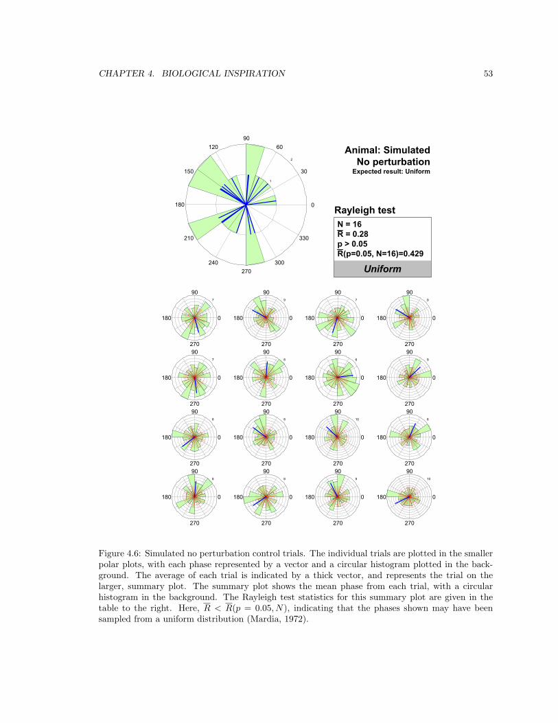
CHAPTER 4. BIOLOGICAL INSPIRATION 53
Crop special 2.2
Usual crop is top and bottom: 2.3375Left and right: 1.4375
Animal: SimulatedNo perturbation
Expected result: Uniform
Close random start stop n
Uniform
Rayleigh testN = 16R = 0.28p > 0.05 R(p=0.05, N=16)=0.429
7
90
270
180 0
9
90
270
180 0
7
90
270
180 0
9
90
270
180 0
7
90
270
180 0
8
90
270
180 0
6
90
270
180 0
9
90
270
180 0
8
90
270
180 0
8
90
270
180 0
10
90
270
180 0
8
90
270
180 0
8
90
270
180 0
8
90
270
180 0
9
90
270
180 0
10
90
270
180 0
1
2
30
210
60
240
90
270
120
300
150
330
180 0
Needd to
Figure 4.6: Simulated no perturbation control trials. The individual trials are plotted in the smallerpolar plots, with each phase represented by a vector and a circular histogram plotted in the back-ground. The average of each trial is indicated by a thick vector, and represents the trial on thelarger, summary plot. The summary plot shows the mean phase from each trial, with a circularhistogram in the background. The Rayleigh test statistics for this summary plot are given in thetable to the right. Here, R < R(p = 0.05, N), indicating that the phases shown may have beensampled from a uniform distribution (Mardia, 1972).
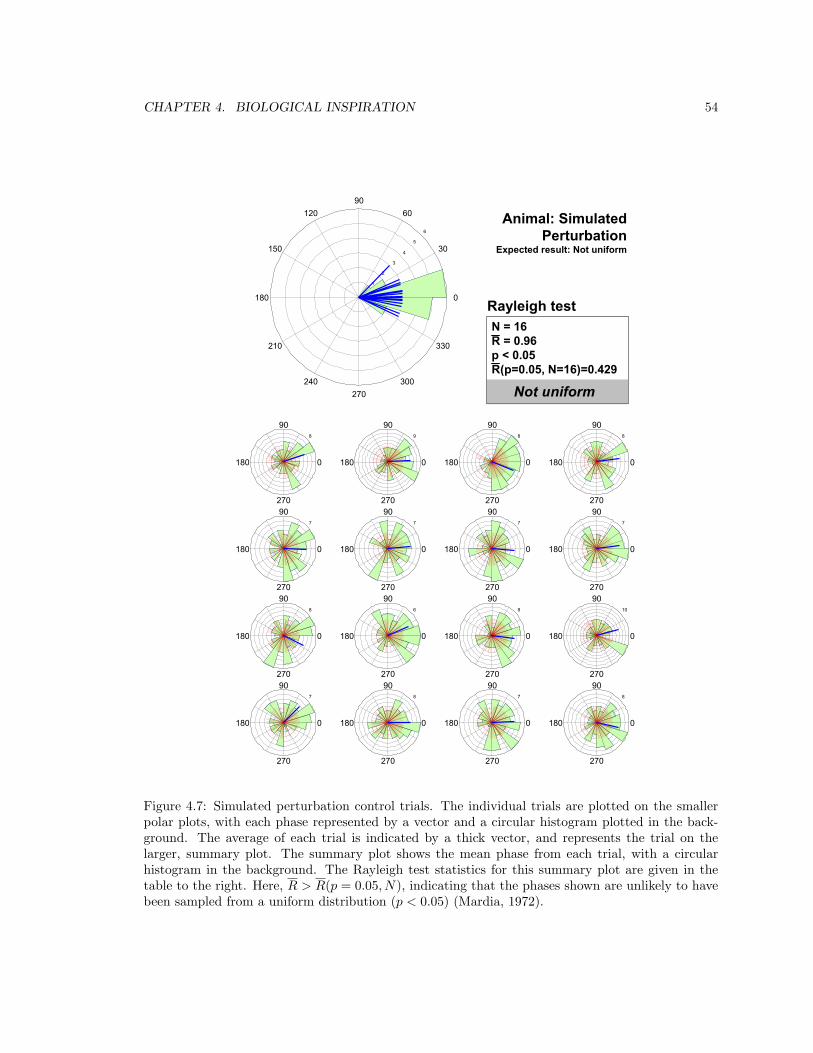
CHAPTER 4. BIOLOGICAL INSPIRATION 54
Crop special 2.2
Usual crop is top and bottom: 2.3375Left and right: 1.4375
Animal: SimulatedPerturbation
Expected result: Not uniform
Close 05 – random start st
Not uniform
Rayleigh testN = 16R = 0.96p < 0.05 R(p=0.05, N=16)=0.429
8
90
270
180 0
9
90
270
180 0
8
90
270
180 0
8
90
270
180 0
7
90
270
180 0
7
90
270
180 0
7
90
270
180 0
7
90
270
180 0
8
90
270
180 0
6
90
270
180 0
8
90
270
180 0
10
90
270
180 0
7
90
270
180 0
8
90
270
180 0
7
90
270
180 0
8
90
270
180 0
1
2
3
4
5
6
30
210
60
240
90
270
120
300
150
330
180 0
Figure 4.7: Simulated perturbation control trials. The individual trials are plotted on the smallerpolar plots, with each phase represented by a vector and a circular histogram plotted in the back-ground. The average of each trial is indicated by a thick vector, and represents the trial on thelarger, summary plot. The summary plot shows the mean phase from each trial, with a circularhistogram in the background. The Rayleigh test statistics for this summary plot are given in thetable to the right. Here, R > R(p = 0.05, N), indicating that the phases shown are unlikely to havebeen sampled from a uniform distribution (p < 0.05) (Mardia, 1972).
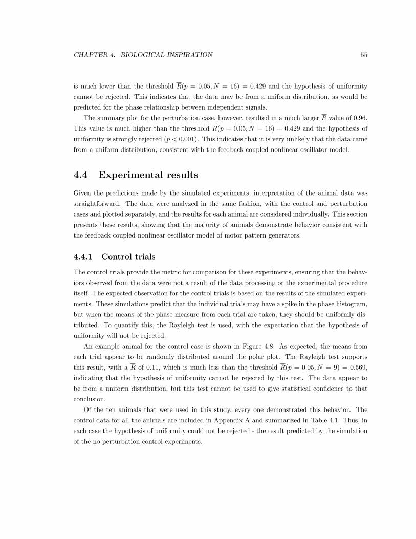
CHAPTER 4. BIOLOGICAL INSPIRATION 55
is much lower than the threshold R(p = 0.05, N = 16) = 0.429 and the hypothesis of uniformity
cannot be rejected. This indicates that the data may be from a uniform distribution, as would be
predicted for the phase relationship between independent signals.
The summary plot for the perturbation case, however, resulted in a much larger R value of 0.96.
This value is much higher than the threshold R(p = 0.05, N = 16) = 0.429 and the hypothesis of
uniformity is strongly rejected (p < 0.001). This indicates that it is very unlikely that the data came
from a uniform distribution, consistent with the feedback coupled nonlinear oscillator model.
4.4 Experimental results
Given the predictions made by the simulated experiments, interpretation of the animal data was
straightforward. The data were analyzed in the same fashion, with the control and perturbation
cases and plotted separately, and the results for each animal are considered individually. This section
presents these results, showing that the majority of animals demonstrate behavior consistent with
the feedback coupled nonlinear oscillator model of motor pattern generators.
4.4.1 Control trials
The control trials provide the metric for comparison for these experiments, ensuring that the behav-
iors observed from the data were not a result of the data processing or the experimental procedure
itself. The expected observation for the control trials is based on the results of the simulated experi-
ments. These simulations predict that the individual trials may have a spike in the phase histogram,
but when the means of the phase measure from each trial are taken, they should be uniformly dis-
tributed. To quantify this, the Rayleigh test is used, with the expectation that the hypothesis of
uniformity will not be rejected.
An example animal for the control case is shown in Figure 4.8. As expected, the means from
each trial appear to be randomly distributed around the polar plot. The Rayleigh test supports
this result, with a R of 0.11, which is much less than the threshold R(p = 0.05, N = 9) = 0.569,
indicating that the hypothesis of uniformity cannot be rejected by this test. The data appear to
be from a uniform distribution, but this test cannot be used to give statistical confidence to that
conclusion.
Of the ten animals that were used in this study, every one demonstrated this behavior. The
control data for all the animals are included in Appendix A and summarized in Table 4.1. Thus, in
each case the hypothesis of uniformity could not be rejected - the result predicted by the simulation
of the no perturbation control experiments.
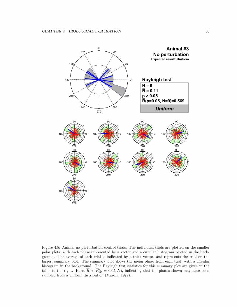
CHAPTER 4. BIOLOGICAL INSPIRATION 56
8
90
270
180 0
8
90
270
180 0
8
90
270
180 0
7
90
270
180 0
6
90
270
180 0
8
90
270
180 0
8
90
270
180 0
7
90
270
180 0
7
90
270
180 0
1
2
30
210
60
240
90
270
120
300
150
330
180 0
Animal #_27_15Hz_no_pert
AllN = 9R/N = 0.11
Animal #3No perturbation
Expected result: Uniform
Uniform
Rayleigh testN = 9R = 0.11p > 0.05 R(p=0.05, N=9)=0.569
Figure 4.8: Animal no perturbation control trials. The individual trials are plotted on the smallerpolar plots, with each phase represented by a vector and a circular histogram plotted in the back-ground. The average of each trial is indicated by a thick vector, and represents the trial on thelarger, summary plot. The summary plot shows the mean phase from each trial, with a circularhistogram in the background. The Rayleigh test statistics for this summary plot are given in thetable to the right. Here, R < R(p = 0.05, N), indicating that the phases shown may have beensampled from a uniform distribution (Mardia, 1972).
CHAPTER 4. BIOLOGICAL INSPIRATION 57
4.4.2 Perturbation trials
In contrast to the control experiments, the feedback coupled nonlinear oscillator model of the motor
pattern generators predicts that the perturbation and EMG signals are related. This expectation is
confirmed by the simulation results which were statistically shown to have a nonuniform distribution,
indicating a relationship between the two signals. Specifically, a spike in the phase histogram is
predicted for each trial, but when the means from each trial are plotted together, the distribution of
these means should be focused, not uniform, which can be quantified by the Rayleigh test. Recall that
positive results show that the animal uses sensory information at the highest speeds of locomotion
and demonstrate behavior consistent with the feedback coupled nonlinear oscillator model of the
motor pattern generators.
The same animal used for Figure 4.8 is used in Figure 4.9 to show the results for the perturbation
case. As was hypothesized with the feedback coupled nonlinear oscillator model, the means from
each trial do not appear to be randomly distributed. Instead, they are focused in a narrow region of
phases, and this is confirmed by the Rayleigh test. The R calculated for this group of trials is 0.89,
which is much greater than the threshold R(p = 0.05, N = 6) = 0.690, rejecting the hypothesis of
uniformity (p < 0.01). This indicates that the data are very unlikely to have come from a uniform
distribution, consistent with the feedback coupled nonlinear oscillator model.
Out of the ten animals that were used in this study, six demonstrated this behavior. The control
data for all the animals are included in Appendix A and summarized in Table 4.1. In addition, out
of the six animals that exhibited this behavior, all of them were significant to the p = 0.01 level,
and four of the six had p-values less than 0.001, strongly rejecting the hypothesis of uniformity.
These results indicate the use of sensory information by the motor pattern generators, even
during the highest speeds of locomotion. In addition, as the results are similar to those predicted by
the simulated experiments, they are consistent with the feedback coupled nonlinear oscillator model
of the motor pattern generators proposed.
However, in four out of the ten animals, the hypothesis of uniformity could not be rejected, which
was not the prediction of the nonlinear oscillator model. For one of these four animals (#5), the R
calculated is very close to the R(p = 0.10, N = 9), indicating a weak relationship may exist. For
the other three animals, the R was much less than the threshold value for even the p = 0.10 level of
significance.
There are several possible reasons for this deviation from the model predictions. Statistically,
varying the level of significance for the Rayleigh test does not appreciably change the results, inspiring
confidence in the measure. While the Rayleigh test seems appropriate, a more detailed statistical
test adept at filtering out more information may yield clearer results.
During the experiments, it was casually noted that some of the animals physically responded to
the perturbation in different ways, a phenomenon that can be expected if the animals are allowed
to behave naturally. Some of the animals continued to run forward, in what seemed to be straight

CHAPTER 4. BIOLOGICAL INSPIRATION 58
7
90
270
180 0
7
90
270
180 0
6
90
270
180 0
6
90
270
180 0
8
90
270
180 0
7
90
270
180 0
1
2
30
210
60
240
90
270
120
300
150
330
180 0
Animal #exp_27_15Hz_pert
AllN = 6R/N = 0.89
Animal #3Perturbation
Expected result: Not uniform
Not uniform
Rayleigh testN = 6R = 0.89p < 0.05 R(p=0.05, N=6)=0.690
Figure 4.9: Animal perturbation trials. The individual trials are plotted on the smaller polar plots,with each phase represented by a vector and a circular histogram plotted in the background. Theaverage of each trial is indicated by a thick vector, and represents the trial on the larger, summaryplot. The summary plot shows the mean phase from each trial, with a circular histogram in thebackground. The Rayleigh test statistics for this summary plot are given in the table to the right.Here, R > R(p = 0.05, N), indicating that the phases shown are unlikely to have been sampled froma uniform distribution (p < 0.05) (Mardia, 1972).
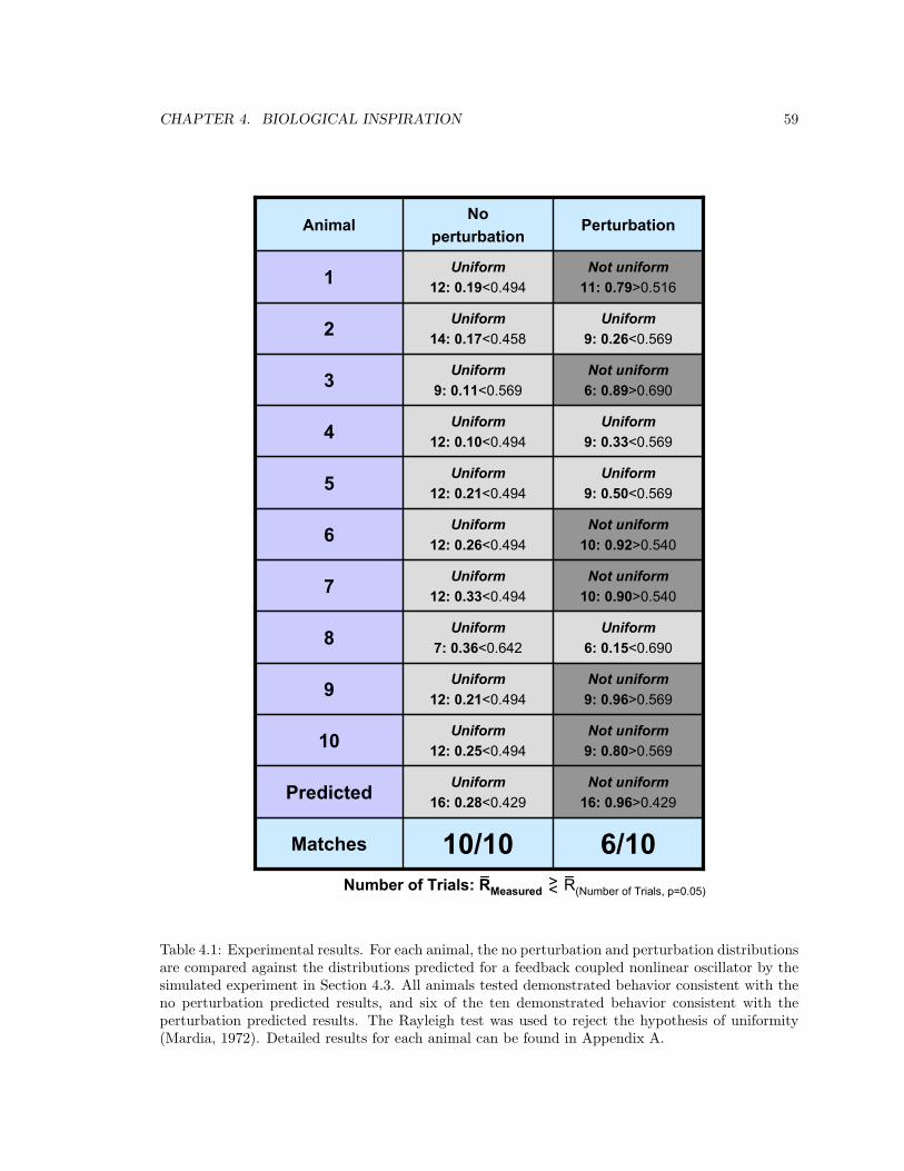
CHAPTER 4. BIOLOGICAL INSPIRATION 59Crop special 2.2
Usual crop is top and bottom: 2.3375Left and right: 1.4375
Uniform6: 0.15<0.690
Uniform7: 0.36<0.6428
Not uniform16: 0.96>0.429
Uniform16: 0.28<0.429Predicted
Not uniform10: 0.92>0.540
Uniform12: 0.26<0.4946
Not uniform10: 0.90>0.540
Uniform12: 0.33<0.4947
Not uniform9: 0.96>0.569
Uniform12: 0.21<0.4949
Not uniform9: 0.80>0.569
Uniform12: 0.25<0.49410
Uniform9: 0.50<0.569
Uniform12: 0.21<0.4945
6/1010/10Matches
Uniform9: 0.33<0.569
Uniform12: 0.10<0.4944
Not uniform6: 0.89>0.690
Uniform9: 0.11<0.5693
Uniform9: 0.26<0.569
Uniform14: 0.17<0.4582
Not uniform11: 0.79>0.516
Uniform12: 0.19<0.4941
PerturbationNo
perturbationAnimal
22242729303132333435Close
N: R<R(p=0.05)
2131221123C
Number of Trials: RMeasured R(Number of Trials, p=0.05)<>
Table 4.1: Experimental results. For each animal, the no perturbation and perturbation distributionsare compared against the distributions predicted for a feedback coupled nonlinear oscillator by thesimulated experiment in Section 4.3. All animals tested demonstrated behavior consistent with theno perturbation predicted results, and six of the ten demonstrated behavior consistent with theperturbation predicted results. The Rayleigh test was used to reject the hypothesis of uniformity(Mardia, 1972). Detailed results for each animal can be found in Appendix A.
CHAPTER 4. BIOLOGICAL INSPIRATION 60
paths. Other animals appeared to want to escape the from the perturbation by turning, which the
spherical inertial treadmill allowed them to do. The analysis has not been performed, but it would
be interesting to see if there is a correlation between the heading consistency and the uniformity (or
lack thereof) observed in the trials.
Finally, this deviation could simply be an aspect of the nervous system that a feedback coupled
nonlinear oscillator model is not able to capture. Wilson (Wilson and Wyman, 1965) also noticed a
similar effect for some animals during his work on locust flight, indicating that there may be other
peripheral mechanisms at work that are not accounted for by these types of models and experiments.
While the locusts used in his study were decapitated, it is still possible that other components of
the nervous system were capable of inhibiting the ability of the sensory feedback circuitry from
responding to the sensory information provided.
While there are many avenues of future work, the most exciting is exploring how such a feedback-
based mechanism affects the dynamics of the locomotion. It is unclear what the functional role
of a feedback coupled nonlinear oscillator-like structure may be. Previous work indicates that a
coordination mechanism is one possible hypothesis, but the range of possibilities is large, and includes
controllers that adaptively respond to changes in the environment (Camhi et al., 1995) (Cohen and
Boothe, 1999).
To explore one part of this large space, this thesis changes focus slightly, from animals to robotics.
Armed with animal experiments that show the use of sensory feedback at high speeds of locomotion
and demonstrate behavior consistent with a feedback coupled nonlinear oscillator model of motor
pattern generators, this thesis addresses how to design these control structures for adaptive control
of cyclic dynamic tasks in changing environments.
In the next chapter, a series of design and analysis tools are presented for creating coupled
systems for adaptive control in changing environments. The usefulness of these tools is demonstrated
in Chapter 6, where a feedback coupled nonlinear oscillator is designed for the biomimetic hexapod
Sprawlita. The biologically inspired controller adaptively responds to changes in the ground slope,
increasing the performance by 33% on uphill slopes. During the process, a better understanding of
the robot locomotion is developed, which in turn may motivate further animal experiments.
Chapter 5
Designing a feedback coupled
nonlinear oscillator for changing
dynamic conditions
It was as if I’d learned to redesign everything, to reshape it so that I saw what ought to
be there, which of course is much inferior to what is there.
-Keith Johnstone (Impro: Improvisation in the theatre)
Animals and robots often perform dynamic cyclic tasks in changing environments. Activities
like walking and running are highly repetitive, but are also clearly influenced by the environments
in which they take place. Walking on sand feels much different than walking on pavement because
it is different. The conditions governing the dynamics of walking are drastically different in the two
circumstances, and the nervous system responds by changing muscle commands accordingly.
As shown in the last two chapters, nonlinear oscillators may be responsible for some of the
sensory-based compensatory responses observed in locomoting animals. Roboticists, especially ones
working on locomotion systems, are interested in how to take advantage of nonlinear oscillators as
controllers. Such feedback coupled nonlinear oscillators are robust to extraneous sensory information
and operate in the absence of sensory failure, as discussed in Chapter 3.
It has been shown that open-loop stable mechanical systems can be made more stable to per-
turbations through feedback coupling to nonlinear oscillators (Miyakoshi et al., 2000) (Schaal and
Atkeson, 1993). It has also been shown that such coupled systems are robust to changes in the en-
vironment, such as changing slopes (Taga et al., 1991) (Taga, 1995) and other changing conditions
(Zhang et al., 2003) (Fukuoka et al., 2003) (Kimura et al., 1999). However, it has not been well
explored and described how to design the feedback coupling and nonlinear oscillator parameters for
61
CHAPTER 5. DESIGNING A FEEDBACK COUPLED NONLINEAR OSCILLATOR 62
such changing conditions. These so-called adaptive controllers sense the change in the environment
and change actuation commands accordingly, resulting in a behavior that would otherwise not exist
through passive mechanical dynamics alone.
This chapter focuses on designing feedback coupled nonlinear oscillator systems, with an emphasis
on analysis and design tools for changing dynamic conditions. First, some of the available nonlinear
oscillator analysis tools are reviewed, using linear analysis tools as a foundation for their introduction.
Then, a visual design technique introduced by Williamson (Williamson, 1999) is explained in Section
5.2, and the available design degrees of freedom are discussed. Next, a simplified model of dynamic
running over changing slope is then examined in detail, motivating the development of further
design and analysis tools: ω contour line analysis, three dimensional visualization, and deliberate
time delays. Finally, the chapter ends with motivations for Chapter 6 and some ideas for future
work.
Throughout this chapter and the next, common nomenclature from controls literature is used.
The mechanical system is referred to as the plant. The nonlinear oscillator, whose inputs are sensor-
based measures of the plant and outputs are actuator commands acting on the plant, is called the
controller. Through these connections, the two components are coupled together and will be referred
to here as the coupled system.
5.1 General tools for design and analysis
The point of mathematical analysis of any system is to characterize and predict the behavior. Some-
times the analysis has an underlying objective: to design a controller which produces a composite
system with a different behavior.
As shown in this section, there are fundamental differences in how linear and nonlinear systems
can be analyzed. Despite these fundamental differences one of the more powerful tools used for
linear systems, the frequency response method, can be adapted for use with nonlinear systems. This
adapted method is called describing function analysis and forms the foundation upon which the
visual design method described in Section 5.2 is based.
5.1.1 Linear systems
While nonlinear mechanical systems are often thought of as the special case, every mechanical system
is nonlinear to some degree, and a “linear” plant actually just refers to a representation that is “good
enough”. Engineers are fortunate that this approximation often is good enough, for these systems
are much easier to analyze than their nonlinear counterparts.
CHAPTER 5. DESIGNING A FEEDBACK COUPLED NONLINEAR OSCILLATOR 63
Superposition
In practice, linear systems are usually identified by system differential equations that are linear
in the state variables. As a definition, however, linear systems are those for which the principle
of superposition applies (Franklin et al., 1994). The desired behavioral predictability results from
superposition - the fact that the aggregate output of the system to a variety of inputs is a linear
combination of the outputs that would result from each input if it were individually applied. In
other words, the system response to one input is not affected by the fact that there are many inputs
- each one is independent of the others.
This simplifies things greatly, because each input can be broken down into a string of impulses,
and the system is convolved with this string to produce the system output in a closed form solution.
This convolution step allows systems to be represented by transfer functions, which lead directly to
Bode plots and other forms of frequency response analyses (Franklin et al., 1994).
Frequency response
Frequency response plots, such as Bode, describe how a system responds to forcing functions of
different frequencies and amplitudes. In these plots, the gain and phase at different forcing function
frequencies are visually represented and are all that is needed to fully describe the steady state
behavior.
The ability to create such concise descriptions is a direct consequence of the superposition princi-
ple. Due to this principle, the amplitude of the input does not affect the gain of the system, and the
frequency at which the linear system responds is always the same as the forcing function frequency.
In other words, the only thing that varies from one linear system to another is how the gain and
phase of the system response change with frequency.
Using frequency response plots in design is extremely powerful for a number of reasons. It is
quite popular in practice because it makes only a few assumptions (such as the system must be
open-loop stable), and none of them pertains to the order of the system (an important consideration
with other methods such as root locus). Additionally, these plots are easy to generate empirically, a
vital property for adapting this method to nonlinear systems. Like other visual methods, frequency
response methods draw upon physical intuition, the ability to imagine and sculpt desired shapes
for design, leaving unnecessary and complicated mathematics behind. This last point becomes
particularly relevant when venturing into the relatively lawless land of nonlinear systems.
5.1.2 Nonlinear systems
Some systems have behavior that is fundamentally nonlinear, such as the nonlinear oscillators de-
scribed in Chapter 3. There are essential characteristics such as stable self-sustained limit cycles
and selective frequency entrainment that cannot be captured by any linearized representation. It is
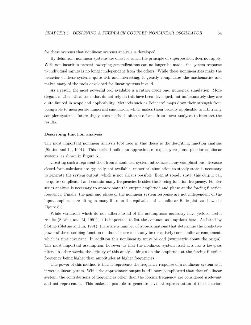
CHAPTER 5. DESIGNING A FEEDBACK COUPLED NONLINEAR OSCILLATOR 64
for these systems that nonlinear systems analysis is developed.
By definition, nonlinear systems are ones for which the principle of superposition does not apply.
With nonlinearities present, sweeping generalizations can no longer be made: the system response
to individual inputs is no longer independent from the others. While these nonlinearities make the
behavior of these systems quite rich and interesting, it greatly complicates the mathematics and
makes many of the tools developed for linear systems invalid.
As a result, the most powerful tool available is a rather crude one: numerical simulation. More
elegant mathematical tools that do not rely on this have been developed, but unfortunately they are
quite limited in scope and applicability. Methods such as Poincare’ maps draw their strength from
being able to incorporate numerical simulation, which makes them broadly applicable to arbitrarily
complex systems. Interestingly, such methods often use forms from linear analyses to interpret the
results.
Describing function analysis
The most important nonlinear analysis tool used in this thesis is the describing function analysis
(Slotine and Li, 1991). This method builds an approximate frequency response plot for nonlinear
systems, as shown in Figure 5.1.
Creating such a representation from a nonlinear system introduces many complications. Because
closed-form solutions are typically not available, numerical simulation to steady state is necessary
to generate the system output, which is not always possible. Even at steady state, this output can
be quite complicated and contain many frequencies besides the forcing function frequency. Fourier
series analysis is necessary to approximate the output amplitude and phase at the forcing function
frequency. Finally, the gain and phase of the nonlinear system response are not independent of the
input amplitude, resulting in many lines on the equivalent of a nonlinear Bode plot, as shown in
Figure 5.3.
While variations which do not adhere to all of the assumptions necessary have yielded useful
results (Slotine and Li, 1991), it is important to list the common assumptions here. As listed by
Slotine (Slotine and Li, 1991), there are a number of approximations that determine the predictive
power of the describing function method. There must only be (effectively) one nonlinear component,
which is time invariant. In addition this nonlinearity must be odd (symmetric about the origin).
The most important assumption, however, is that the nonlinear system itself acts like a low-pass
filter. In other words, the efficacy of this analysis hinges on the amplitude at the forcing function
frequency being higher than amplitudes at higher frequencies.
The power of this method is that it represents the frequency response of a nonlinear system as if
it were a linear system. While the approximate output is still more complicated than that of a linear
system, the contributions of frequencies other than the forcing frequency are considered irrelevant
and not represented. This makes it possible to generate a visual representation of the behavior,
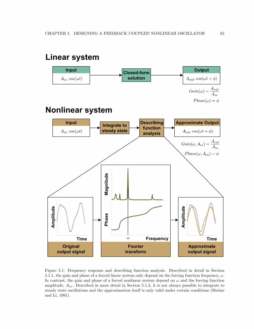
CHAPTER 5. DESIGNING A FEEDBACK COUPLED NONLINEAR OSCILLATOR 65Crop special 2.2
Usual crop is top and bottom: 2.3375Left and right: 1.4375
Closed-formsolution
Input Integrate Output
Input
Linear system
Integrate
Output
Integrate tosteady state
Input
Nonlinear systemApproximate OutputDescribing
functionanalysis
Originaloutput signal
Time
Am
plitu
de
Approximateoutput signal
Am
plitu
de
Time
Mag
nitu
dePh
ase
Fouriertransform
Frequency
These plots from 2004_04_22b
Figure 5.1: Frequency response and describing function analysis. Described in detail in Section5.1.1, the gain and phase of a forced linear system only depend on the forcing function frequency, ω.In contrast, the gain and phase of a forced nonlinear system depend on ω and the forcing functionamplitude, Ain. Described in more detail in Section 5.1.2, it is not always possible to integrate tosteady state oscillations and the approximation itself is only valid under certain conditions (Slotineand Li, 1991).
CHAPTER 5. DESIGNING A FEEDBACK COUPLED NONLINEAR OSCILLATOR 66
which is crucial for this thesis.
There are a number of techniques that can be used to integrate to steady state. Nominally,
the analyses in this thesis integrate until the state variables are within a percent range of the same
point during the previous cycle, thus determining that steady state has been reached. Williamson
took a slightly different approach, and integrated for fixed amounts of time, checking at the end
to make sure that the nonlinear oscillator frequency and forcing function frequency were within a
range of one another (Williamson, personal communication). Additionally, a hybrid of these two
methods is used for this thesis in Chapter 6. In all implementations, conditions were set to identify
cases in which steady state solutions at the forcing function frequency were not possible. These
cases were eliminated, as the inability to reach steady state indicated that entrainment did not
occur. Generally, this lack of entrainment was due to insufficient input amplitude for the distance of
the forcing function frequency from the self-sustained limit cycle frequency, as discussed in Section
3.2.2. Owing to the approximate nature of this method, the results from the various entrainment
identification techniques were found to be functionally quite similar.
The remainder of this chapter examines and extends a method introduced by Williamson
(Williamson, 1999) for designing coupled systems with nonlinear oscillators using the describing
function method. Chapter 6 then applies this method to a biologically-inspired hexapedal robot. In
that chapter, some alternative describing function analysis methods that largely violate the basic
assumptions are developed and presented there.
5.2 Design with a feedback coupled nonlinear oscillator: a
visual method
The work in this thesis toward designing a feedback coupled nonlinear oscillator is largely motivated
by the work of Williamson (Williamson, 1999). Motivated by studies of human arm movement, he
developed a technique to control a robotic arm with a coupled nonlinear oscillator to perform a
variety of cyclic dynamic tasks. This work was novel as it represented the plant and the controller
dynamics visually, and this visualization was used to predict the coupled system behavior. While
design was not the focus, suggestions were made for adjusting each of these dynamics, toward
affecting the overall system behavior. In this regard it is the precursor to the work done in this
thesis.
5.2.1 System architecture
While others have thought of feedback coupling nonlinear oscillators to control dynamic systems
interacting with various environments (Taga et al., 1991) (Taga, 1995) (Schaal and Sternad, 1998)
(Lewis et al., 2003) (Lewis et al., 2000) (Lewis, 1996), Williamson (Williamson, 1999) captured the

CHAPTER 5. DESIGNING A FEEDBACK COUPLED NONLINEAR OSCILLATOR 67
essence of the structure that this thesis adopts, as shown in Figure 5.2a. Instead of a true plant and
controller structure, the two components are thought of as two systems with their own dynamics.
Connected together, they become a coupled system with a composite set of dynamics different than
each system in isolation.
The nonlinear oscillator controller dynamics generate an arm trajectory without an external
reference signal. Like more traditional error-based controllers, the feedback to the controller does
affect the output, but it is indirect and through the dynamics of the nonlinear oscillator. This
sensory feedback was generally joint position, but could have been any cyclic sensory information
as Williamson also experimented with velocity and force feedback.
5.2.2 The graphical design method
The method that Williamson developed is an extension of the frequency response method for linear
systems described in Section 5.1 and the describing function method for nonlinear systems discussed
in Section 5.1.2. As shown in Figure 5.3e, each system is graphically represented on the same plot
and the predicted solution can be found visually. Additionally, alternate solutions can be found
by changing the parameters of each system, which results in different system “shapes”. Design is
therefore visually intuitive and abstracted away from the (complicated) underlying mathematics.
The basic idea is that for a coupled system, the overall loop gain is unity and the loop phase is
zero. Therefore, by plotting the s-plane representations of the plant and the inverse of the controller,
the solution can be found at the intersection. At this point, the gain, phase, and frequency of
each system are the same, meaning that the gain and phase conditions are met at that particular
frequency. Nyquist techniques can be used to examine the stability of the solution as in (Slotine and
Li, 1991), but stability was found not to be a concern for the systems considered in this thesis.
In the s-plane, the real and imaginary components of the gain and phase are plotted on orthogonal
axes. Gain is the radius from the origin, and phase is the counterclockwise angle from the positive
real axis. By plotting the inverse of the controller, the reciprocal of the gain and the negative of
the phase are shown. Though important for finding the intersection point, the frequencies of each
system cannot be represented visually, and are typically labeled directly.
Like other design processes, this procedure is iterative, and there are many options available as
shown in Figure 5.4. The power of visualizing the systems is that changes are represented graphically,
and the impact on the overall solution can be seen. In the following sections, the shapes of the plant
and the controller are modified by adjusting the parameters of each system.
5.2.3 Shaping the plant and controller: Adjusting gains
The simplest changes in shape are the result of modifying the input and output gains of the plant
and the controller. While there are four gains that can be changed, some of them are redundant, as
shown in Figure 5.5.
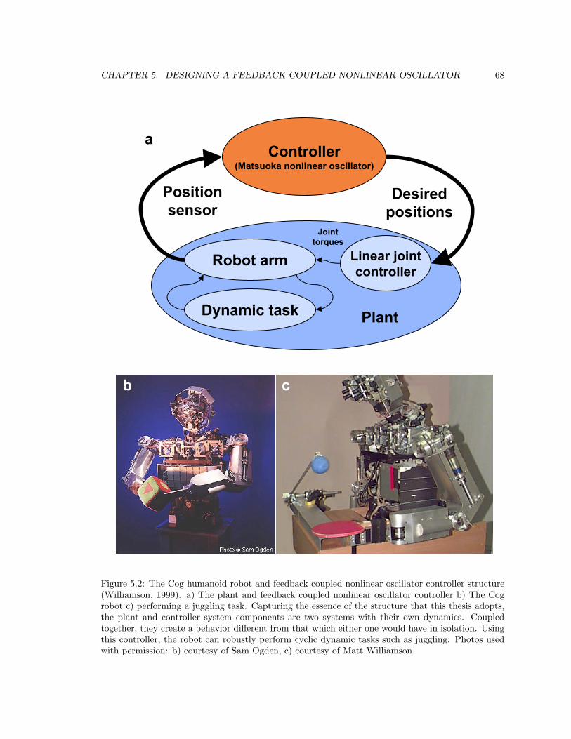
CHAPTER 5. DESIGNING A FEEDBACK COUPLED NONLINEAR OSCILLATOR 68Crop special 2.2
Usual crop is top and bottom: 2.3375Left and right: 1.4375
Controller(Matsuoka nonlinear oscillator)
Robot arm
Desiredpositions
Positionsensor
Linear jointcontroller
PlantDynamic task
a
b c
Jointtorques
Figure 5.2: The Cog humanoid robot and feedback coupled nonlinear oscillator controller structure(Williamson, 1999). a) The plant and feedback coupled nonlinear oscillator controller b) The Cogrobot c) performing a juggling task. Capturing the essence of the structure that this thesis adopts,the plant and controller system components are two systems with their own dynamics. Coupledtogether, they create a behavior different from that which either one would have in isolation. Usingthis controller, the robot can robustly perform cyclic dynamic tasks such as juggling. Photos usedwith permission: b) courtesy of Sam Ogden, c) courtesy of Matt Williamson.
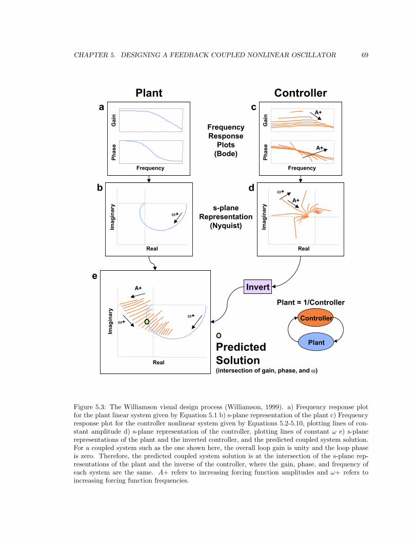
CHAPTER 5. DESIGNING A FEEDBACK COUPLED NONLINEAR OSCILLATOR 69
Crop special 2.2
Usual crop is top and bottom: 2.3375Left and right: 1.4375
Invert
Plant Controller
FrequencyResponse
Plots(Bode)
s-planeRepresentation
(Nyquist)
PredictedSolution
Plant = 1/Controller
Gai
n
Frequency
Phas
e
Gai
n
Frequency
Phas
e
A+
A+
ω+
Real
Imag
inar
y
A+ω+
Real
Imag
inar
y
ω+ω+
A+
Real
Imag
inar
y
These plots from 2004_04_22c (I think)
(intersection of gain, phase, and ω)
Controller
Plant
a
b
e
c
d
FASTFigure 5.3: The Williamson visual design process (Williamson, 1999). a) Frequency response plotfor the plant linear system given by Equation 5.1 b) s-plane representation of the plant c) Frequencyresponse plot for the controller nonlinear system given by Equations 5.2-5.10, plotting lines of con-stant amplitude d) s-plane representation of the controller, plotting lines of constant ω e) s-planerepresentations of the plant and the inverted controller, and the predicted coupled system solution.For a coupled system such as the one shown here, the overall loop gain is unity and the loop phaseis zero. Therefore, the predicted coupled system solution is at the intersection of the s-plane rep-resentations of the plant and the inverse of the controller, where the gain, phase, and frequency ofeach system are the same. A+ refers to increasing forcing function amplitudes and ω+ refers toincreasing forcing function frequencies.
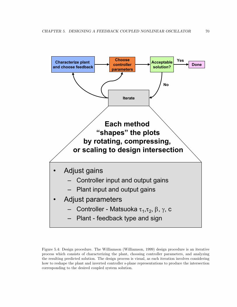
CHAPTER 5. DESIGNING A FEEDBACK COUPLED NONLINEAR OSCILLATOR 70Crop special 2.2
Usual crop is top and bottom: 2.3375Left and right: 1.4375
Choosecontroller
parameters
Characterize plant and choose feedback
Nonlinear system
Iterate
Acceptablesolution?
• Adjust gains– Controller input and output gains– Plant input and output gains
• Adjust parameters– Controller - Matsuoka τ1,τ2, β, γ, c– Plant - feedback type and sign
Each method “shapes” the plots
by rotating, compressing, or scaling to design intersection
No
DoneYes
Figure 5.4: Design procedure. The Williamson (Williamson, 1999) design procedure is an iterativeprocess which consists of characterizing the plant, choosing controller parameters, and analyzingthe resulting predicted solution. The design process is visual, as each iteration involves consideringhow to reshape the plant and inverted controller s-plane representations to produce the intersectioncorresponding to the desired coupled system solution.
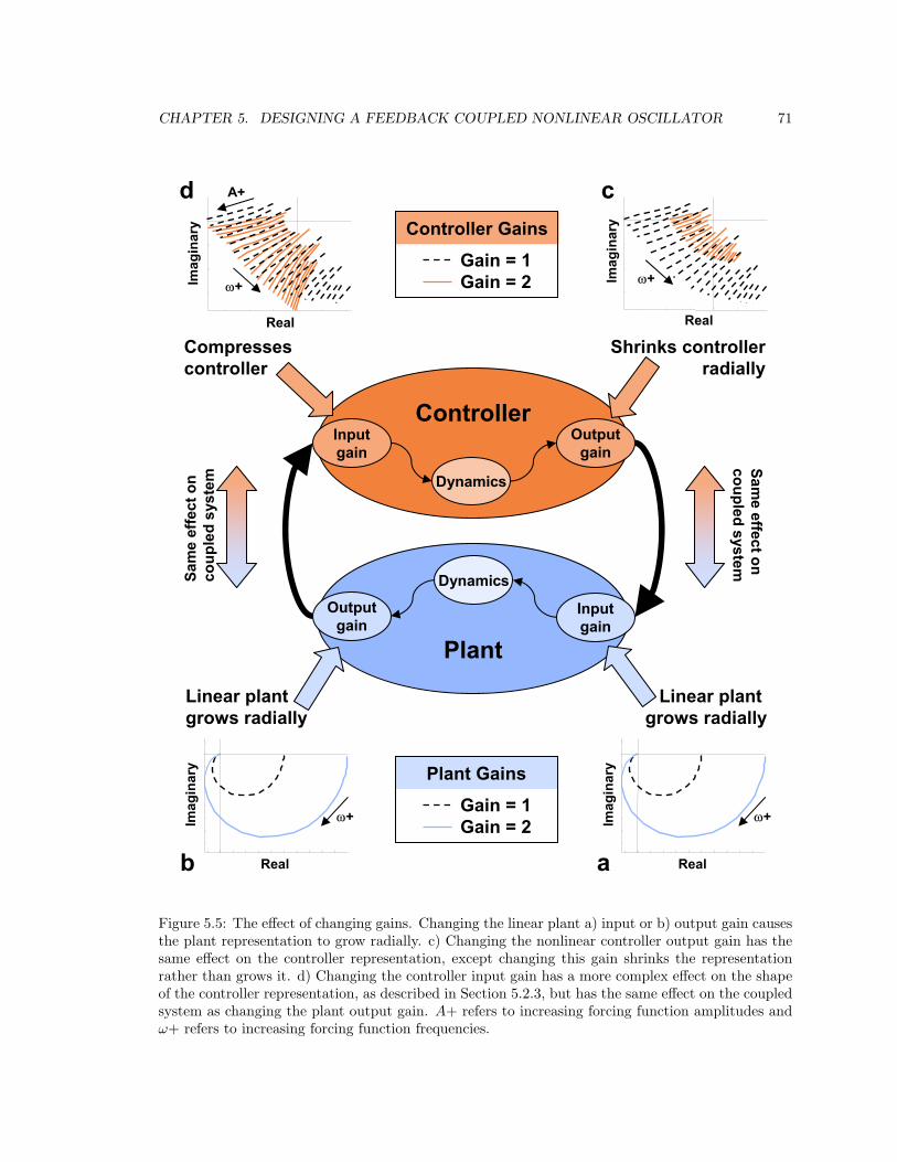
CHAPTER 5. DESIGNING A FEEDBACK COUPLED NONLINEAR OSCILLATOR 71Crop special 2.2
Usual crop is top and bottom: 2.3375Left and right: 1.4375
Outputgain
Inputgain
Outputgain
Inputgain
Dynamics
Controller
Dynamics
Plant
Compressescontroller
Shrinks controllerradially
Linear plant grows radially
Linear plant grows radially
-1.5 -1 -0.5
-1.5
-1
-0.5
0
-0.5 0 0.5 1
1 1.2 1.4 1.6 1.8
Same effect on
coupled system
Sam
e ef
fect
on
coup
led
syst
em
These plots from 2004_04_23c
ω+
Real
Imag
inar
y
A+
ω+
Real
Imag
inar
y
Gain = 1Gain = 2
Controller Gains
Gain = 1Gain = 2
Plant Gains
ω+
Real
Imag
inar
y
ω+
Real
Imag
inar
y
Background gray these?
b
cd
a
Figure 5.5: The effect of changing gains. Changing the linear plant a) input or b) output gain causesthe plant representation to grow radially. c) Changing the nonlinear controller output gain has thesame effect on the controller representation, except changing this gain shrinks the representationrather than grows it. d) Changing the controller input gain has a more complex effect on the shapeof the controller representation, as described in Section 5.2.3, but has the same effect on the coupledsystem as changing the plant output gain. A+ refers to increasing forcing function amplitudes andω+ refers to increasing forcing function frequencies.
CHAPTER 5. DESIGNING A FEEDBACK COUPLED NONLINEAR OSCILLATOR 72
For a linear plant, the input and output gains have the same effect and both simply increase the
plant output amplitude for a given input amplitude. Thus, the overall plant gain increases with an
increase in either input or output gain. When this effect is plotted in the s-plane, the effect is that
the radius of the plant representation grows as the input or output gains are increased, as shown in
Figure 5.5a,b.
It should be noted that if the plant were not linear, then these two gains would not have the
same effect. In this chapter, the plant is always linear. In the next chapter, however, the model of
the plant is nonlinear and these two gains have different effects, which will be discussed there.
Similar to the plant gains, changing the output gain on the controller simply changes the radius
of the visual representation, as shown in Figure 5.5c. In this case, since the inverse of the controller is
plotted, the radius shrinks with increasing gain. While this does change the shape of the controller,
it is redundant in that the same coupled system effect could be obtained by increasing the input
gain on the plant. In other words, shrinking the controller is the same as growing the plant - the
coupled system is affected in the same way.
The only gain that does not simply grow or shrink the visual representation is the controller
input gain, called hj in Equations 5.2-5.10 for the Matsuoka oscillator (Matsuoka, 1985) (Matsuoka,
1987). This is due to the nonlinearity of the controller, as the behavior changes with different input
amplitudes. Thus, the controller does not grow or shrink with increasing input gain, but instead
is compressed near the origin, as shown in Figure 5.5d. This compression results from high input
amplitude behaviors at lower input amplitudes, or in other words, larger radii behavior occurring at
smaller radii.
To further complicate the situation, the entrainment region (i.e. the region in frequency space
for which entrainment occurs) is increased with the input gain. Therefore, larger input gains also
increase the number of possible solutions, as frequencies further away from the self-sustained limit
cycle frequency of the oscillator become candidate solution frequencies. Although it may not be
clear given these complications, changing this gain has the same effect on the coupled system as
changing the output gain of the plant, as indicated in Figure 5.5.
It is important to also keep in mind that, with the exception of the entrainment region, changing
any of the gains does not affect the characteristics of either system individually. For example, the
nonlinear oscillator self-sustained limit cycle frequency is the same and the dynamic characteristics
of the plant are also unaffected. Changing the gains only affects the coupling strength between the
two systems, and therefore the coupled system behavior.
5.2.4 Shaping the plant: Rotations by negation, derivatives
Another way of shaping the plant that does not affect the inherent dynamic characteristics is by
using derivatives and negations of the state variables. Williamson (Williamson, 1999) mostly focused
on position feedback, but showed that velocity and force feedback were also viable alternatives.
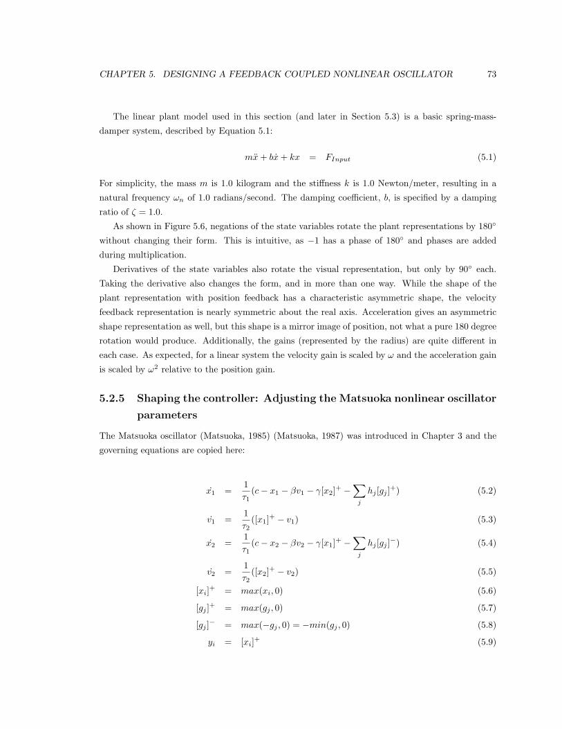
CHAPTER 5. DESIGNING A FEEDBACK COUPLED NONLINEAR OSCILLATOR 73
The linear plant model used in this section (and later in Section 5.3) is a basic spring-mass-
damper system, described by Equation 5.1:
mx + bx + kx = FInput (5.1)
For simplicity, the mass m is 1.0 kilogram and the stiffness k is 1.0 Newton/meter, resulting in a
natural frequency ωn of 1.0 radians/second. The damping coefficient, b, is specified by a damping
ratio of ζ = 1.0.
As shown in Figure 5.6, negations of the state variables rotate the plant representations by 180◦
without changing their form. This is intuitive, as −1 has a phase of 180◦ and phases are added
during multiplication.
Derivatives of the state variables also rotate the visual representation, but only by 90◦ each.
Taking the derivative also changes the form, and in more than one way. While the shape of the
plant representation with position feedback has a characteristic asymmetric shape, the velocity
feedback representation is nearly symmetric about the real axis. Acceleration gives an asymmetric
shape representation as well, but this shape is a mirror image of position, not what a pure 180 degree
rotation would produce. Additionally, the gains (represented by the radius) are quite different in
each case. As expected, for a linear system the velocity gain is scaled by ω and the acceleration gain
is scaled by ω2 relative to the position gain.
5.2.5 Shaping the controller: Adjusting the Matsuoka nonlinear oscillator
parameters
The Matsuoka oscillator (Matsuoka, 1985) (Matsuoka, 1987) was introduced in Chapter 3 and the
governing equations are copied here:
x1 =1τ1
(c− x1 − βv1 − γ[x2]+ −∑
j
hj [gj ]+) (5.2)
v1 =1τ2
([x1]+ − v1) (5.3)
x2 =1τ1
(c− x2 − βv2 − γ[x1]+ −∑
j
hj [gj ]−) (5.4)
v2 =1τ2
([x2]+ − v2) (5.5)
[xi]+ = max(xi, 0) (5.6)
[gj ]+ = max(gj , 0) (5.7)
[gj ]− = max(−gj , 0) = −min(gj , 0) (5.8)
yi = [xi]+ (5.9)
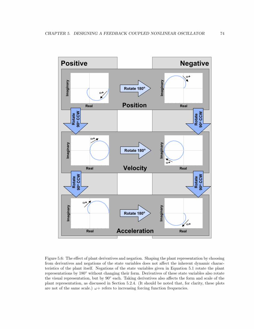
CHAPTER 5. DESIGNING A FEEDBACK COUPLED NONLINEAR OSCILLATOR 74
Crop special 2.2
Usual crop is top and bottom: 2.3375
Negative
Derivatives are also scaled by ω
These plots from 2004_04_23c
Positive
Position
Rotate 180o
Real
Imag
inar
y
Real
Imag
inar
y
Velocity
Rotate 180o
Real
Imag
inar
y
Real
Imag
inar
y
Acceleration
Rotate 180o
Real
Imag
inar
y
Real
Imag
inar
y
Rot
ate
90o
CC
W
Rot
ate
90o
CC
WR
otat
e90
oC
CW
Rot
ate
90o
CC
W
ω+
ω+
ω+
ω+
ω+
ω+
Figure 5.6: The effect of plant derivatives and negation. Shaping the plant representation by choosingfrom derivatives and negations of the state variables does not affect the inherent dynamic charac-teristics of the plant itself. Negations of the state variables given in Equation 5.1 rotate the plantrepresentations by 180◦ without changing their form. Derivatives of these state variables also rotatethe visual representation, but by 90◦ each. Taking derivatives also affects the form and scale of theplant representation, as discussed in Section 5.2.4. (It should be noted that, for clarity, these plotsare not of the same scale.) ω+ refers to increasing forcing function frequencies.
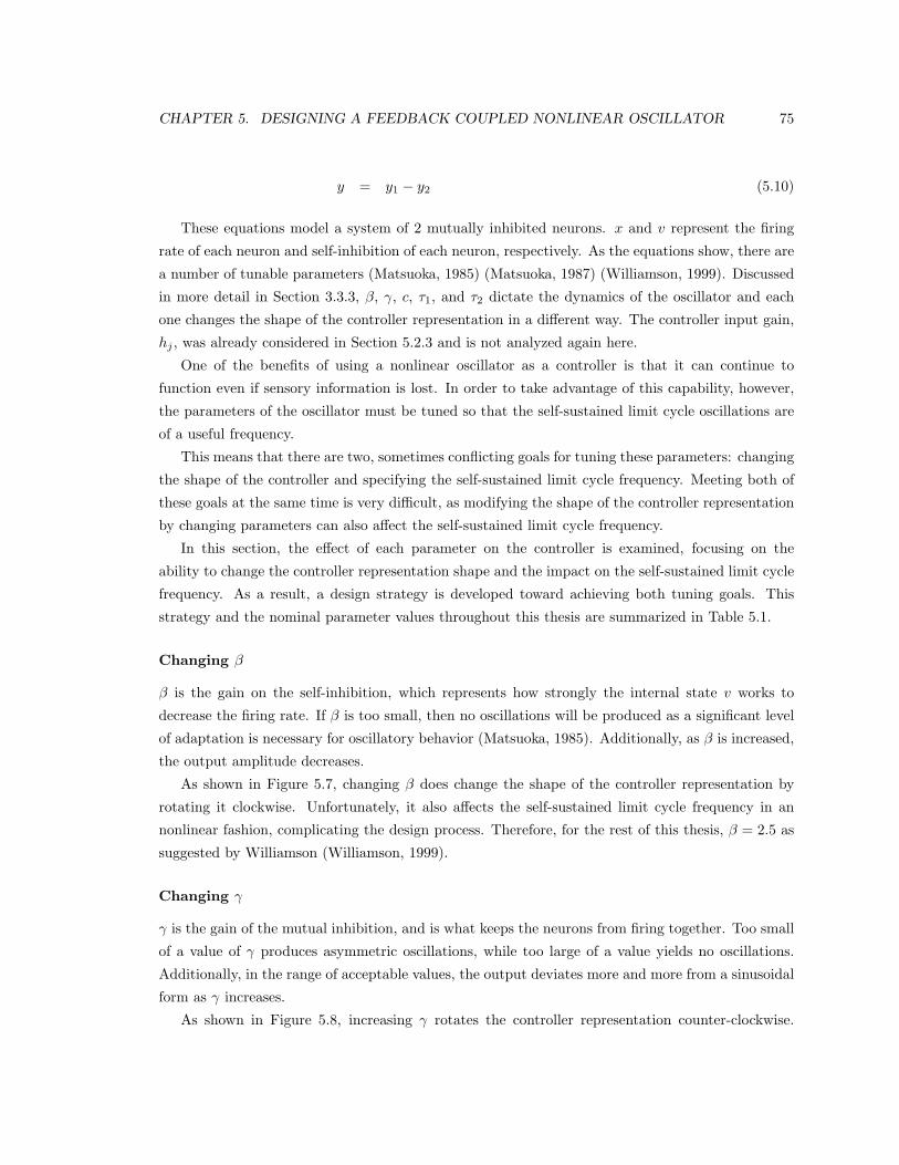
CHAPTER 5. DESIGNING A FEEDBACK COUPLED NONLINEAR OSCILLATOR 75
y = y1 − y2 (5.10)
These equations model a system of 2 mutually inhibited neurons. x and v represent the firing
rate of each neuron and self-inhibition of each neuron, respectively. As the equations show, there are
a number of tunable parameters (Matsuoka, 1985) (Matsuoka, 1987) (Williamson, 1999). Discussed
in more detail in Section 3.3.3, β, γ, c, τ1, and τ2 dictate the dynamics of the oscillator and each
one changes the shape of the controller representation in a different way. The controller input gain,
hj , was already considered in Section 5.2.3 and is not analyzed again here.
One of the benefits of using a nonlinear oscillator as a controller is that it can continue to
function even if sensory information is lost. In order to take advantage of this capability, however,
the parameters of the oscillator must be tuned so that the self-sustained limit cycle oscillations are
of a useful frequency.
This means that there are two, sometimes conflicting goals for tuning these parameters: changing
the shape of the controller and specifying the self-sustained limit cycle frequency. Meeting both of
these goals at the same time is very difficult, as modifying the shape of the controller representation
by changing parameters can also affect the self-sustained limit cycle frequency.
In this section, the effect of each parameter on the controller is examined, focusing on the
ability to change the controller representation shape and the impact on the self-sustained limit cycle
frequency. As a result, a design strategy is developed toward achieving both tuning goals. This
strategy and the nominal parameter values throughout this thesis are summarized in Table 5.1.
Changing β
β is the gain on the self-inhibition, which represents how strongly the internal state v works to
decrease the firing rate. If β is too small, then no oscillations will be produced as a significant level
of adaptation is necessary for oscillatory behavior (Matsuoka, 1985). Additionally, as β is increased,
the output amplitude decreases.
As shown in Figure 5.7, changing β does change the shape of the controller representation by
rotating it clockwise. Unfortunately, it also affects the self-sustained limit cycle frequency in an
nonlinear fashion, complicating the design process. Therefore, for the rest of this thesis, β = 2.5 as
suggested by Williamson (Williamson, 1999).
Changing γ
γ is the gain of the mutual inhibition, and is what keeps the neurons from firing together. Too small
of a value of γ produces asymmetric oscillations, while too large of a value yields no oscillations.
Additionally, in the range of acceptable values, the output deviates more and more from a sinusoidal
form as γ increases.
As shown in Figure 5.8, increasing γ rotates the controller representation counter-clockwise.
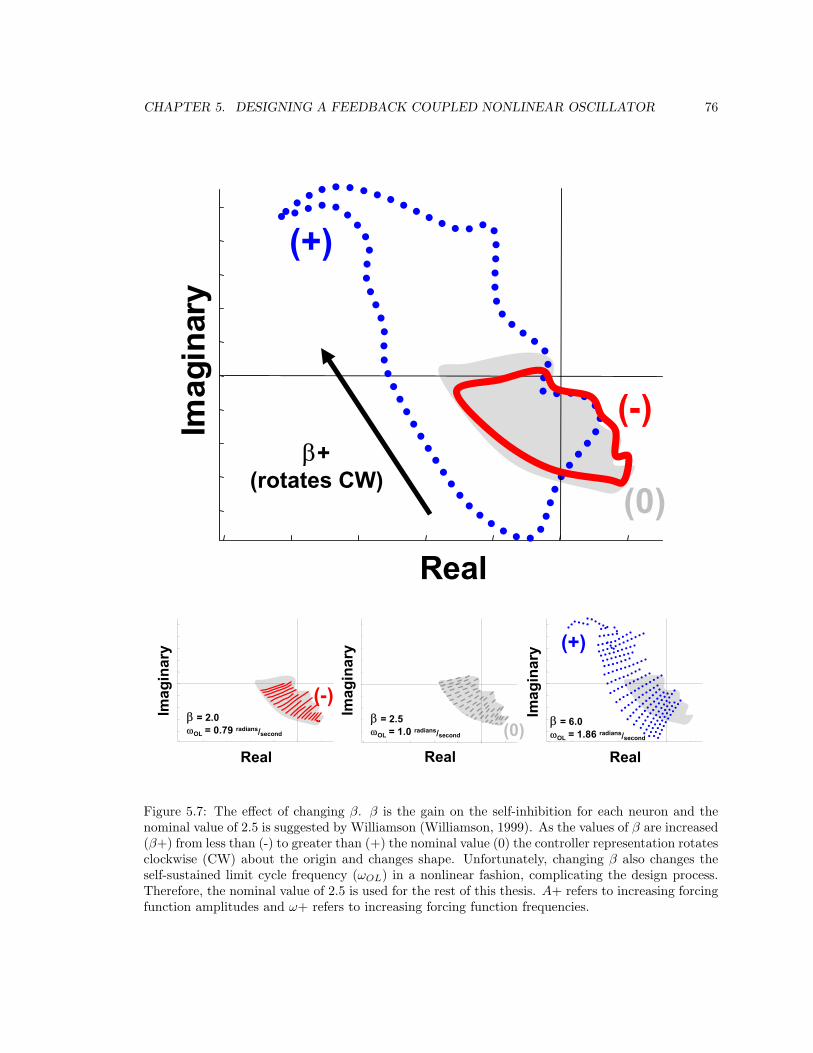
CHAPTER 5. DESIGNING A FEEDBACK COUPLED NONLINEAR OSCILLATOR 76
Crop special 2.2
Usual crop is top and bottom: 2.3375Left and right: 1.4375
-5 -4 -3 -2 -1 0 1
-2
-1.5
-1
-0.5
0
0.5
1
1.5
2
2.5 Beta is adaptation, and is limited at the low eIn general, Beta rotates the plots clockwise
These plots from 2004_04_23c
LineGrayDasBlob
Imag
inar
y
Real
β = 2.0ωOL = 0.79 radians/second
αβχδεφγηιϕκλµνοπθρστυϖωξψζ
Imag
inar
y
Real
β = 2.5ωOL = 1.0 radians/second
Imag
inar
y
Real
β = 6.0ωOL = 1.86 radians/second
UneDotsRedAddCut
Imag
inar
y
Real
β+(rotates CW)
(-)
(+)
(0)
(-)(0)
(+)
Figure 5.7: The effect of changing β. β is the gain on the self-inhibition for each neuron and thenominal value of 2.5 is suggested by Williamson (Williamson, 1999). As the values of β are increased(β+) from less than (-) to greater than (+) the nominal value (0) the controller representation rotatesclockwise (CW) about the origin and changes shape. Unfortunately, changing β also changes theself-sustained limit cycle frequency (ωOL) in a nonlinear fashion, complicating the design process.Therefore, the nominal value of 2.5 is used for the rest of this thesis. A+ refers to increasing forcingfunction amplitudes and ω+ refers to increasing forcing function frequencies.
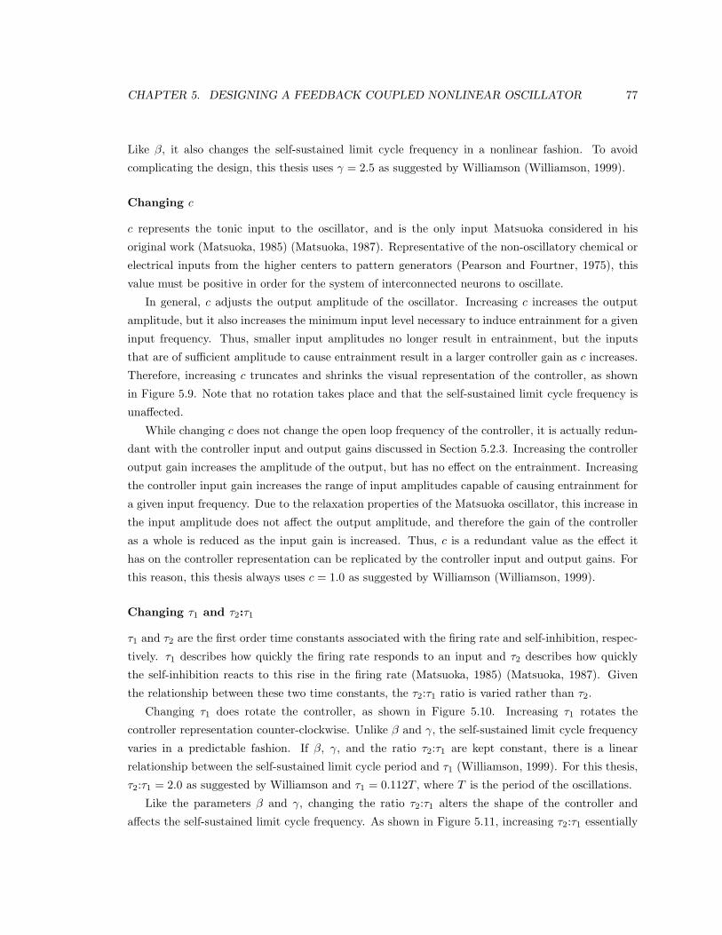
CHAPTER 5. DESIGNING A FEEDBACK COUPLED NONLINEAR OSCILLATOR 77
Like β, it also changes the self-sustained limit cycle frequency in a nonlinear fashion. To avoid
complicating the design, this thesis uses γ = 2.5 as suggested by Williamson (Williamson, 1999).
Changing c
c represents the tonic input to the oscillator, and is the only input Matsuoka considered in his
original work (Matsuoka, 1985) (Matsuoka, 1987). Representative of the non-oscillatory chemical or
electrical inputs from the higher centers to pattern generators (Pearson and Fourtner, 1975), this
value must be positive in order for the system of interconnected neurons to oscillate.
In general, c adjusts the output amplitude of the oscillator. Increasing c increases the output
amplitude, but it also increases the minimum input level necessary to induce entrainment for a given
input frequency. Thus, smaller input amplitudes no longer result in entrainment, but the inputs
that are of sufficient amplitude to cause entrainment result in a larger controller gain as c increases.
Therefore, increasing c truncates and shrinks the visual representation of the controller, as shown
in Figure 5.9. Note that no rotation takes place and that the self-sustained limit cycle frequency is
unaffected.
While changing c does not change the open loop frequency of the controller, it is actually redun-
dant with the controller input and output gains discussed in Section 5.2.3. Increasing the controller
output gain increases the amplitude of the output, but has no effect on the entrainment. Increasing
the controller input gain increases the range of input amplitudes capable of causing entrainment for
a given input frequency. Due to the relaxation properties of the Matsuoka oscillator, this increase in
the input amplitude does not affect the output amplitude, and therefore the gain of the controller
as a whole is reduced as the input gain is increased. Thus, c is a redundant value as the effect it
has on the controller representation can be replicated by the controller input and output gains. For
this reason, this thesis always uses c = 1.0 as suggested by Williamson (Williamson, 1999).
Changing τ1 and τ2:τ1
τ1 and τ2 are the first order time constants associated with the firing rate and self-inhibition, respec-
tively. τ1 describes how quickly the firing rate responds to an input and τ2 describes how quickly
the self-inhibition reacts to this rise in the firing rate (Matsuoka, 1985) (Matsuoka, 1987). Given
the relationship between these two time constants, the τ2:τ1 ratio is varied rather than τ2.
Changing τ1 does rotate the controller, as shown in Figure 5.10. Increasing τ1 rotates the
controller representation counter-clockwise. Unlike β and γ, the self-sustained limit cycle frequency
varies in a predictable fashion. If β, γ, and the ratio τ2:τ1 are kept constant, there is a linear
relationship between the self-sustained limit cycle period and τ1 (Williamson, 1999). For this thesis,
τ2:τ1 = 2.0 as suggested by Williamson and τ1 = 0.112T , where T is the period of the oscillations.
Like the parameters β and γ, changing the ratio τ2:τ1 alters the shape of the controller and
affects the self-sustained limit cycle frequency. As shown in Figure 5.11, increasing τ2:τ1 essentially
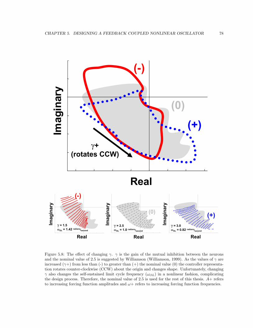
CHAPTER 5. DESIGNING A FEEDBACK COUPLED NONLINEAR OSCILLATOR 78Crop special 2.2
Usual crop is top and bottom: 2.3375Left and right: 1.4375
Gamma is mutual inhibition, and is limited at the low end and the high endIn general, Gammarotates the plots
-2 -1.5 -1 -0.5 0 0.5 1 1.5-2
-1.5
-1
-0.5
0
0.5
1
These plots from 2004_04_23cαβχδεφγηιϕκλµνοπθρστυϖωξψζ
Imag
inar
y
Real
γ = 2.5ωOL = 1.0 radians/second
γ = 3.0ωOL = 0.82 radians/second
Imag
inar
y
Real
γ = 1.5ωOL = 1.42 radians/second
Imag
inar
y
Real
Imag
inar
y
Real
γ+(rotates CCW)
(-)
(+)
(-)
(0)
(+)
(0)
Figure 5.8: The effect of changing γ. γ is the gain of the mutual inhibition between the neuronsand the nominal value of 2.5 is suggested by Williamson (Williamson, 1999). As the values of γ areincreased (γ+) from less than (-) to greater than (+) the nominal value (0) the controller representa-tion rotates counter-clockwise (CCW) about the origin and changes shape. Unfortunately, changingγ also changes the self-sustained limit cycle frequency (ωOL) in a nonlinear fashion, complicatingthe design process. Therefore, the nominal value of 2.5 is used for the rest of this thesis. A+ refersto increasing forcing function amplitudes and ω+ refers to increasing forcing function frequencies.

CHAPTER 5. DESIGNING A FEEDBACK COUPLED NONLINEAR OSCILLATOR 79
Crop special 2.2
Usual crop is top and bottom: 2.3375Left and right: 1.4375
C is the constant input to the oscillatorThe only input considered by Matsuoka (8Adjusts the output of the oscillator, and adjust the minimum input level necessary(makes it harder as amplitude goes up)
These plots from 2004_04_23c
Real
Imag
inar
y
c = 0.5ωOL = 1.0 radians/second
Imag
inar
y
Real
c = 1.0ωOL = 1.0 radians/second
Imag
inar
y
Real
c = 2.0ωOL = 1.0 radians/second
Imag
inar
y
Real
c+(truncates & shrinks)
(-)
(+)
(0)
(-)(0)
(+)
Figure 5.9: The effect of changing c. c is the tonic input to each of the neurons and the nominalvalue of 1.0 is suggested by Williamson (Williamson, 1999). As the values of c are increased (c+)from less than (-) to greater than (+) the nominal value (0) the controller representation is truncatedand shrunk radially. Changing c does not have any affect on the self-sustained limit cycle frequency(ωOL). However, c is redundant with the controller input and output gains. Therefore, the nominalvalue of 1.0 is used for the rest of this thesis. A+ refers to increasing forcing function amplitudesand ω+ refers to increasing forcing function frequencies.
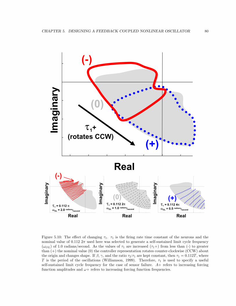
CHAPTER 5. DESIGNING A FEEDBACK COUPLED NONLINEAR OSCILLATOR 80Crop special 2.2
Usual crop is top and bottom: 2.3375Left and right: 1.4375
Tau1 is the time neuron time constanHow the membrane changes (how leaChanges self-sustained limit cycle frConstant relationship with period if tTau1 = .112 T) if Tau2/Tau1 = 2
These plots from 2004_04_23cIm
agin
ary
Real
τ1 = 0.112 πωOL = 2.0 radians/second
αβχδεφγηιϕκλµνοπθρστυϖωξψζ
Imag
inar
y
Real
τ1 = 0.112 2πωOL = 1.0 radians/second
Imag
inar
y
Real
τ1 = 0.112 4πωOL = 0.5 radians/second
UneDotRedAddCut
(+) 0(-)
Imag
inar
y
Real
τ1+(rotates CCW)
(-)
(+)
(0)
(-)
(0)
(+)
Figure 5.10: The effect of changing τ1. τ1 is the firing rate time constant of the neurons and thenominal value of 0.112 2π used here was selected to generate a self-sustained limit cycle frequency(ωOL) of 1.0 radians/second. As the values of τ1 are increased (τ1+) from less than (-) to greaterthan (+) the nominal value (0) the controller representation rotates counter-clockwise (CCW) aboutthe origin and changes shape. If β, γ, and the ratio τ2:τ1 are kept constant, then τ1 = 0.112T , whereT is the period of the oscillations (Williamson, 1999). Therefore, τ1 is used to specify a usefulself-sustained limit cycle frequency for the case of sensor failure. A+ refers to increasing forcingfunction amplitudes and ω+ refers to increasing forcing function frequencies.
CHAPTER 5. DESIGNING A FEEDBACK COUPLED NONLINEAR OSCILLATOR 81
rotates the controller representation counter-clockwise. In addition, the ratio τ2:τ1 also changes the
self-sustained limit cycle frequency in a nonlinear fashion. To maintain the τ1 and T relationship
above, this thesis uses τ2:τ1 = 2.0 as suggested by Williamson (Williamson, 1999).
Summary
The effect of each of the controller parameters on the shape of the controller representation is
summarized in Table 5.1. τ1 is an effective design parameter as it is used to specify an appropriate
self-sustained limit cycle frequency for the event of sensor failure using the simple, linear relationship
τ1 = 0.112T , where T is the self-sustained limit cycle period (Williamson, 1999).
Once τ1 has been selected, β, γ, and the τ2:τ1 = 2.0 ratio cannot be changed, as they also affect
the self-sustained limit cycle frequency. The only remaining parameter is c, but this is redundant
with the controller input and output gains. These limitations make it very difficult to shape the
controller by using these parameters, motivating the need for other methods as discussed in the next
section.
5.2.6 Design considerations
Overall, the tunable parameters discussed do provide some degrees of freedom for design. Gains
can grow, shrink and compress the shapes of the plots, and taking derivatives and negations rotates
them. Each of these shaping methods is considered viable, as it does not affect the underlying
dynamics of either the plant or the controller.
Unfortunately, though, there is no method for achieving fine rotations. Derivatives and negations
rotate the plant by 90◦ and 180◦, respectively, which is quite drastic. Summarized in Table 5.1,
changing the controller parameters rotates the controller in finer increments, but at the cost of
changing the underlying dynamics of the controller itself, and results in undesired changes in the
self-sustained limit cycle frequency.
Therefore, it is desirable to have a tool that provides more gentle rotations of the plant or con-
troller, so that the visual intersection point (and therefore the coupled system solution) can be
fine-tuned. A novel technique for achieving this is discussed later in Section 5.3.4. First, how-
ever, the following section explores how systems with changing dynamic conditions are represented.
Williamson touched on this topic in his thesis (Williamson, 1999), but emphasized robustness, not
adaptation in general. This thesis focuses on this subject, with the intent of using the feedback cou-
pled nonlinear oscillator to create arbitrary adaptive behaviors in response to changing conditions.
5.3 Designing for changing dynamic conditions
This thesis focuses on design for adaptation - how to design a controller to produce specific behavioral
changes in response to varying conditions. This section uses an example system to develop tools for
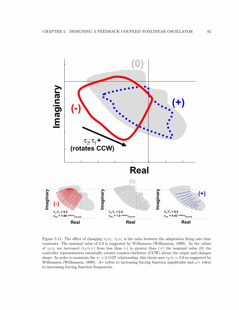
CHAPTER 5. DESIGNING A FEEDBACK COUPLED NONLINEAR OSCILLATOR 82
Crop special 2.2
Usual crop is top and bottom: 2.3375Left and right: 1.4375
These plots from 2004_04_23cIm
agin
ary
Real
τ2:τ1 = 0.5ωOL = 1.98 radians/second
Imag
inar
y
Real
τ2:τ1 = 2.0ωOL = 1.0 radians/second
Imag
inar
y
Real
τ2:τ1 = 8.0ωOL = 0.42 radians/second
(+)(-)
(0)
Imag
inar
y
Real
τ2:τ1+(rotates CCW)
(-) (+)
(0)
Figure 5.11: The effect of changing τ2:τ1. τ2:τ1 is the ratio between the adaptation firing rate timeconstants. The nominal value of 2.0 is suggested by Williamson (Williamson, 1999). As the valuesof τ2:τ1 are increased (τ2:τ1+) from less than (-) to greater than (+) the nominal value (0) thecontroller representation essentially rotates counter-clockwise (CCW) about the origin and changesshape. In order to maintain the τ1 = 0.112T relationship, this thesis uses τ2:τ1 = 2.0 as suggested byWilliamson (Williamson, 1999). A+ refers to increasing forcing function amplitudes and ω+ refersto increasing forcing function frequencies.
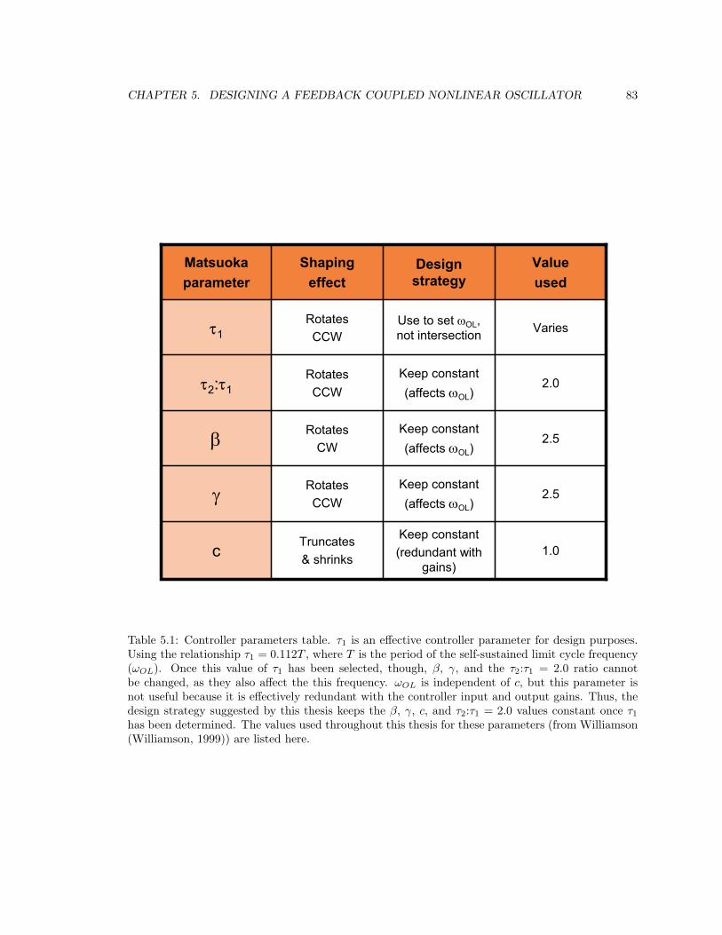
CHAPTER 5. DESIGNING A FEEDBACK COUPLED NONLINEAR OSCILLATOR 83
Usual crop is top and bottom: 2.3375Left and right: 1.4375
-2.5 -2 -1.5 -1 -0.5 0 0.5-2
-1.5
-1
-0.5
0
0.5
Tau1 is the time neuron timeHow the membrane changesChanges self-sustained limitConstant relationship with pTau1 = 112 T) if Tau2/Tau1 =
These plots from 2004_04_23c
1.0Keep constant(redundant with
gains)
Truncates& shrinksc
2.5Keep constant(affects ωOL)
RotatesCCWγ
2.5Keep constant(affects ωOL)
RotatesCWβ
2.0Keep constant(affects ωOL)
RotatesCCWτ2:τ1
VariesUse to set ωOL, not intersection
RotatesCCWτ1
Valueused
Design strategy
Shapingeffect
Matsuokaparameter
Table 5.1: Controller parameters table. τ1 is an effective controller parameter for design purposes.Using the relationship τ1 = 0.112T , where T is the period of the self-sustained limit cycle frequency(ωOL). Once this value of τ1 has been selected, though, β, γ, and the τ2:τ1 = 2.0 ratio cannotbe changed, as they also affect the this frequency. ωOL is independent of c, but this parameter isnot useful because it is effectively redundant with the controller input and output gains. Thus, thedesign strategy suggested by this thesis keeps the β, γ, c, and τ2:τ1 = 2.0 values constant once τ1
has been determined. The values used throughout this thesis for these parameters (from Williamson(Williamson, 1999)) are listed here.
CHAPTER 5. DESIGNING A FEEDBACK COUPLED NONLINEAR OSCILLATOR 84
using a feedback coupled nonlinear oscillator to create such an adaptive controller.
For the examples given here and in the next chapter, the desired adaptive behavior is assumed
to be known a priori, specified by the designer. For example, the desired adaptive behavior for
the robot in Chapter 6 is a change in locomotion frequency in response to varying ground slopes.
While the ultimate effect of this adaptive behavior is toward maintaining forward velocity despite
these slope changes, the design procedure and tools developed are for creating arbitrary adaptive
behaviors, not ones limited to regulation.
In contrast, Williamson (Williamson, 1999) did not focus on design for arbitrary adaptive be-
haviors, but concentrated on demonstrating a single specific behavior, robustness - constant behav-
ior/performance despite changes in oscillator and environmental parameters. He stated that his
main objective was to exploit the natural dynamics of the system he was controlling by using the
nonlinear oscillator to drive the system at resonance. In general, he found that the feedback to the
nonlinear oscillator did seem to result in the entire system operating at what he determined to be
the mechanical resonance, and showed this behavior for a number of tasks ranging from juggling to
hammering a nail.
The behavior most relevant to this thesis was a wood sawing exercise. The robot arm moved a
saw back and forth over a piece of wood, and as it encountered different sections the frequency of the
robot changed accordingly. While the behavior was not likely designed for and how it came about
was not analyzed in further detail, it describes the basic motivation for exploring coupled nonlinear
oscillators as an adaptive controller - that the feedback coupled nonlinear oscillator does not just
create a system that is more robust than open-loop, it can actually create an adaptive one.
5.3.1 Example: A simplified model of running over changing slopes
While it does not even come close to capturing the complexities of dynamic running, this section
uses a very simplified model of running over slopes as an example system, shown in Figure 5.12. The
main salient points that this model does attempt to capture are that running is a cyclic dynamic
phenomenon, and that varying conditions alter the plant dynamics. The focus of this section is to
develop tools to analyze how the feedback coupled nonlinear oscillator changes the behavior of this
example system in response to these variations.
In particular, one of the adjustable parameters for the biologically-inspired robot in Chapter 6 is
the open-loop frequency (Cham et al., 2000), which has been shown to have an important influence
on robot performance (Clark et al., 2001). Because this system is already quite stable in the face
of large short-duration perturbations, the intended benefit of the coupled nonlinear oscillator is to
adjust the open loop frequency to best suit the long-term general dynamic environment. Thus, when
analyzing the behavior of the simple system in this chapter, the focus is on how the frequency of
operation changes with varying dynamic conditions.
As running is a cyclic dynamic phenomenon (Full and Koditschek, 1999) (Full and Tu, 1991)
CHAPTER 5. DESIGNING A FEEDBACK COUPLED NONLINEAR OSCILLATOR 85
(Full and Tu, 1990), the basic model is a spring-mass-damper system shown in Figure 5.12 and
described by Equation 5.11:
mx + bx + kx = FInput (5.11)
For simplicity, the mass m is 1.0 kilogram and the stiffness k is 1.0 Newton/meter, resulting in a
natural frequency ωn of 1.0 radian/second. The damping coefficient, b, is varied to approximate
running on slopes and is specified by the damping ratio ζ. Running on flat ground corresponds to
a damping ratio (ζ) of 1. For uphill running, ζ is greater than one, and more energy is removed
from the system during each “stride”. Downhill running corresponds to a ζ value of less than one,
resulting in less damping and less energy dissipated per cycle.
As this is solely for example purposes, the feedback to the oscillator is arbitrarily chosen to
be the mass displacement from equilibrium. There are some basic requirements on the controller
input, which are discussed briefly by Matsuoka (Matsuoka, 1985) (Matsuoka, 1987) and Williamson
(Williamson, 1999). Since the input is split into positive and negative components (see Equations
5.2 - 5.10), the input should generally be symmetric about zero. Usually, this can be achieved by
high-pass filtering, which removes any zero frequency components. Another method for removing
bias is to subtract any contralateral contribution (i.e. left-right) if available, a method that is used
in Chapter 6.
The result of varying the external dynamic conditions changes representation of the linear plant
from a single line to a series of lines on the s-plane visualization. As shown in Figure 5.13a, this
means that there are now also a series of solutions, one for each value of ζ that is considered. Again,
these solutions are found where the gain, phase, and ω of the plant and inverse controller are equal.
ω can not be represented visually so each line is labeled accordingly.
The behavior of the coupled system is shown in Figure 5.13b. As ζ changes, the frequency of the
coupled system changes as well due to the different dynamic conditions and the feedback coupling.
At high and low ζ values, the frequency is lower than for ζ values near 1. In order to design behaviors
such as this, it is important to understand how they come about.
5.3.2 ω contour analysis
As stated before, the three values that must match for the plant and the inverted controller to
intersect are gain, phase, and ω. While difficult to visualize on the two dimensional plots, the ω
contribution is very important. To help visualize this, Figure 5.14a includes additional lines on the
plant to visualize lines of constant ω as ζ changes.
Figure 5.14a also zooms in on the relevant part of the s-plane visual representation. There are
three distinct regions of the intersection solution, where the relative angles of the ω contour lines
of the plant and inverted controller cross. These relative angles result in the behavior observed
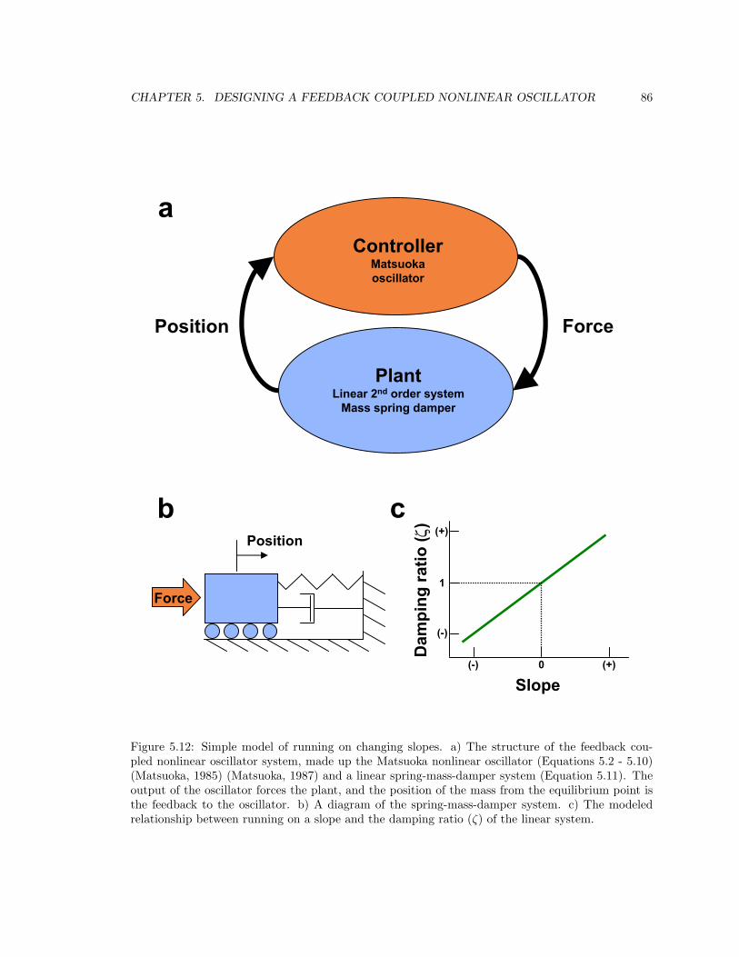
CHAPTER 5. DESIGNING A FEEDBACK COUPLED NONLINEAR OSCILLATOR 86Crop special 2.2
Usual crop is top and bottom: 2.3375Left and right: 1.4375
MSy
ControllerMatsuokaoscillator
PlantLinear 2nd order system
Mass spring damper
Position Force
Position
Force
Slope
Dam
ping
ratio
(ζ)
0
1
(+)(-)
(-)
(+)
a
b c
Figure 5.12: Simple model of running on changing slopes. a) The structure of the feedback cou-pled nonlinear oscillator system, made up the Matsuoka nonlinear oscillator (Equations 5.2 - 5.10)(Matsuoka, 1985) (Matsuoka, 1987) and a linear spring-mass-damper system (Equation 5.11). Theoutput of the oscillator forces the plant, and the position of the mass from the equilibrium point isthe feedback to the oscillator. b) A diagram of the spring-mass-damper system. c) The modeledrelationship between running on a slope and the damping ratio (ζ) of the linear system.
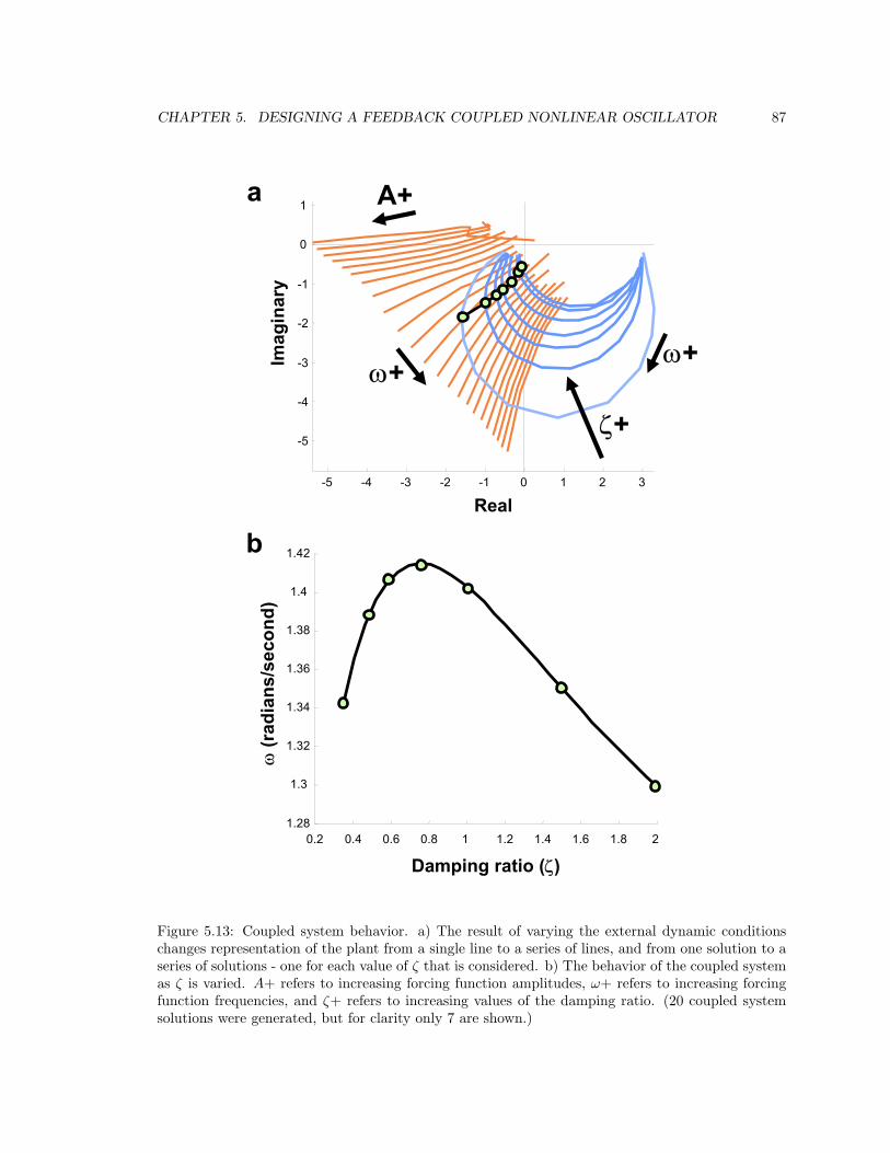
CHAPTER 5. DESIGNING A FEEDBACK COUPLED NONLINEAR OSCILLATOR 87Crop special 2.2
Usual crop is top and bottom: 2.3375Left and right: 1.4375
SolutionTrend
Plant output gain = 3Curve actually generated
These plots from 2004_04_24a,b
ζ+
-5 -4 -3 -2 -1 0 1 2 3
-5
-4
-3
-2
-1
0
1
Real
Imag
inar
y
Damping ratio (ζ)
ω(r
adia
ns/s
econ
d)
0.2 0.4 0.6 0.8 1 1.2 1.4 1.6 1.8 21.28
1.3
1.32
1.34
1.36
1.38
1.4
1.42
ω+
A+
ω+
a
b
Figure 5.13: Coupled system behavior. a) The result of varying the external dynamic conditionschanges representation of the plant from a single line to a series of lines, and from one solution to aseries of solutions - one for each value of ζ that is considered. b) The behavior of the coupled systemas ζ is varied. A+ refers to increasing forcing function amplitudes, ω+ refers to increasing forcingfunction frequencies, and ζ+ refers to increasing values of the damping ratio. (20 coupled systemsolutions were generated, but for clarity only 7 are shown.)
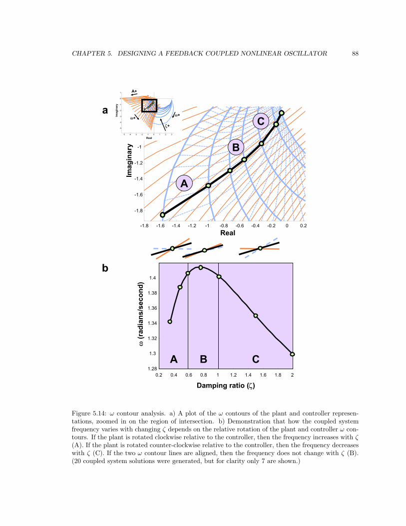
CHAPTER 5. DESIGNING A FEEDBACK COUPLED NONLINEAR OSCILLATOR 88
Crop special 2.2
Usual crop is top and bottom: 2.3375Left and right: 1.4375
These plots from 2004_04_24d
-1.8 -1.6 -1.4 -1.2 -1 -0.8 -0.6 -0.4 -0.2 0 0.2
-1.8
-1.6
-1.4
-1.2
-1
-0.8
-0.6
A
B
Cζ+
-5 -4 -3 -2 -1 0 1 2 3
-5
-4
-3
-2
-1
0
1
Real
Imag
inar
yω+
A+
ω+
Real
Imag
inar
y
Damping ratio (ζ)
ω(r
adia
ns/s
econ
d)
0.2 0.4 0.6 0.8 1 1.2 1.4 1.6 1.8 21.28
1.3
1.32
1.34
1.36
1.38
1.4
A B C
Missing # is 1.42
Plant output gain = 3Curve actually generated
a
b
Figure 5.14: ω contour analysis. a) A plot of the ω contours of the plant and controller represen-tations, zoomed in on the region of intersection. b) Demonstration that how the coupled systemfrequency varies with changing ζ depends on the relative rotation of the plant and controller ω con-tours. If the plant is rotated clockwise relative to the controller, then the frequency increases with ζ(A). If the plant is rotated counter-clockwise relative to the controller, then the frequency decreaseswith ζ (C). If the two ω contour lines are aligned, then the frequency does not change with ζ (B).(20 coupled system solutions were generated, but for clarity only 7 are shown.)
CHAPTER 5. DESIGNING A FEEDBACK COUPLED NONLINEAR OSCILLATOR 89
in Figure 5.14b. The clear relationship established here is that if the plant is rotated clockwise
relative to the inverted controller, then the coupled system frequency increases with ζ. Conversely,
if the plant is rotated counter-clockwise relative to the inverted controller, then the coupled system
frequency decreases with ζ. If the two ω contour lines are essentially aligned, then the coupled
system frequency is not greatly affected by ζ. These cases are labeled in Figure 5.14 by A, C, and
B, respectively.
5.3.3 Three dimensional visualization
As shown in the previous section, the ω contour lines are extremely useful in determining the solution
behavior. Like a topographical map, these contours describe the elevation of each visual representa-
tion. The solution also changes in elevation, in this case much like the pass at the intersection of two
mountains. This is not simply a convenient way to think of the solution behavior, as the solution is
at the intersection of three variables, not just two. Therefore, plotting these visual representations in
three dimensional space results in a truer representation than the two dimensional plots commonly
used.
Bringing this visualization into three dimensions is extremely powerful. Previously, design con-
sisted of changing two dimensional shapes and guessing at the ω component for the intersection.
With the three dimensional representation, the shapes are now surfaces in three dimensional space
and the intersection is easy to see, as shown in Figure 5.15.
It should be emphasized that by adopting this visualization, nothing is fundamentally changed.
The coupled system is governed by the same equations regardless of how it is visualized. The effects
of changes discussed in Section 5.2 still are still the same, and the changes in shape that they induce
can easily be converted to three dimensions.
The power of this visualization is being able to more intuitively describe what the solution
behavior is and what changes in shape need to occur to get the behavior desired. The following
section describes a method to get one such change in shape: fine scale rotations through intentional
time delays.
5.3.4 Shaping the controller: Fine scale rotations through intentional
time delays
It is clear to see from Figure 5.15 that simply rotating the plant or inverted controller about the ω
axis will produce a different solution intersection. In this case, as the inverted controller is rotated
counter-clockwise, the frequency of the solution will decrease, as the two surfaces will intersect at
a lower elevation, corresponding to a lower ω. The details of the behavior still depend on the (ω
contour-based) details of the intersection, but fine scale rotations are needed to get the two surfaces
into the desired ω solution range.
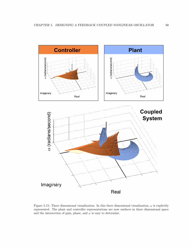
CHAPTER 5. DESIGNING A FEEDBACK COUPLED NONLINEAR OSCILLATOR 90Crop special 2.2
Usual crop is top and bottom: 2.3375Left and right: 1.4375
PlantController
on
These plots from 2004_04_24e
Plant output g
CoupledSystem
Figure 5.15: Three dimensional visualization. In this three dimensional visualization, ω is explicitlyrepresented. The plant and controller representations are now surfaces in three dimensional spaceand the intersection of gain, phase, and ω is easy to determine.
CHAPTER 5. DESIGNING A FEEDBACK COUPLED NONLINEAR OSCILLATOR 91
Gains alone typically do not help in this regard, as they generally only grow and shrink the shapes
of the plant and inverted controller, which are generally already radially oriented. Derivatives and
negations do rotate the shapes of the plant and inverted controller about the ω axis, but by relatively
drastic amounts. Changes in the controller parameters were shown to induce subtle rotations about
the ω axis, but at the expense of changing the underlying dynamics of the nonlinear oscillator, an
undesirable effect.
What is truly desired to rotate these shapes is a pure phase delay operator. The angle about the
ω axis is the phase of each system, and adding in an arbitrary phase delay would rotate the plant
clockwise and the inverted controller counter-clockwise. Of course, a phase advance would rotate
the systems in the opposite direction, but is not possible for nondeterministic real systems.
Unfortunately, for the same reasons, a pure phase delay is not possible either. Such an element
requires knowledge of the instantaneous period of the coupled system, but this cannot be known
before it occurs. Therefore, a close approximation to such an element is an intentional time delay.
The word intentional is included for the reason that in most engineering control systems, delay
causes control problems and is avoided. It is interesting to note that this is not the case for biological
systems, as significant delays exist at every level, and have even been shown to have crucial roles
(Carr and Konishi, 1990).
While the actual location does not affect the coupled system behavior, in this thesis the inten-
tional time delay is inserted in the controller, as shown in Figure 5.16. As it is an approximation to
the pure phase delay, the effect of the intentional time delay is not a simple rotation of the inverted
controller. At low frequencies, the intentional time delay imparts a small change in phase, while at
higher frequencies, the resultant phase delay is much larger. The effect of this is that the shape is
not only rotated, but it is also “spread”, which is also shown in Figure 5.16.
Figure 5.17 shows how the solution of the coupled system changes with increasing intentional
time delay. As this delay increases, the controller is rotated and spread counter-clockwise, resulting
in the two surfaces intersecting at lower elevations, as shown in Figure 5.17c. The changing solution
ω range can be seen in Figure 5.17a.
In addition, the behavior of the solution changes with increasing intentional time delays, as would
be predicted by the ω contour analysis. The intersection occurs at different locations on the surfaces
as the inverted controller is rotated, and the changes in the contours result in different dynamic
responses to the changing ζ conditions.
The following chapter designs a feedback coupled nonlinear oscillator for a much more complex
robot model, one that has been shown to capture the essential characteristics of a real biomimetic
robot, Sprawlita. Over the course of designing a controller for this simulation-based model, the
analytical and design tools developed in this chapter are used. Additionally, new techniques are
developed for dealing with the specific control commands necessary for driving the robot and further
visualization tools are developed. Feedback signals are studied and processed in such a way that
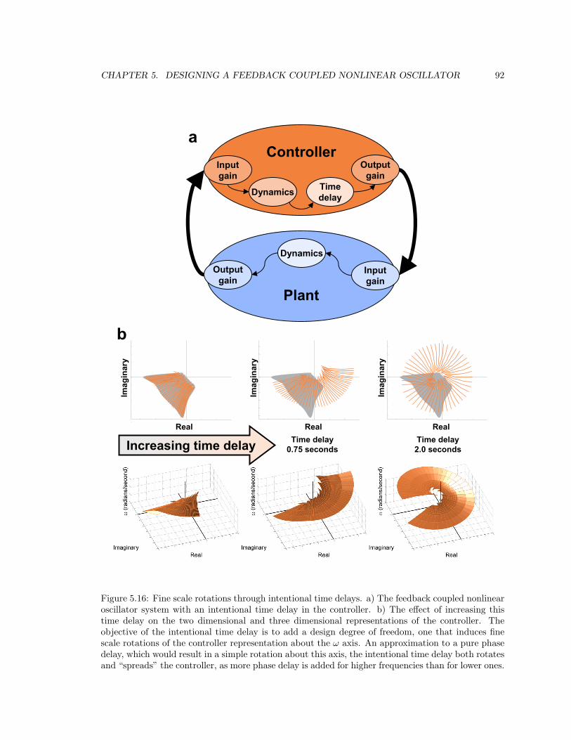
CHAPTER 5. DESIGNING A FEEDBACK COUPLED NONLINEAR OSCILLATOR 92
Crop special 2.2
Usual crop is top and bottom: 2.3375Left and right: 1.4375
ates and “spreads”
Get axes same Also include the trendSince that changes?That is a lot of work…
These plots from 2004_04_24f
Plant output gain = 3
Outputgain
Inputgain
Outputgain
Inputgain
Dynamics
Controller
Dynamics
Plant
Timedelay
a
b
Fix omega nad rad/sec
Real
Imag
inar
y
Real
Imag
inar
y
Real
Imag
inar
y
Time delay0.75 seconds
Time delay2.0 secondsIncreasing time delay
Figure 5.16: Fine scale rotations through intentional time delays. a) The feedback coupled nonlinearoscillator system with an intentional time delay in the controller. b) The effect of increasing thistime delay on the two dimensional and three dimensional representations of the controller. Theobjective of the intentional time delay is to add a design degree of freedom, one that induces finescale rotations of the controller representation about the ω axis. An approximation to a pure phasedelay, which would result in a simple rotation about this axis, the intentional time delay both rotatesand “spreads” the controller, as more phase delay is added for higher frequencies than for lower ones.

CHAPTER 5. DESIGNING A FEEDBACK COUPLED NONLINEAR OSCILLATOR 93
Crop special 2.2
Usual crop is top and bottom: 2.3375Left and right: 1.4375otates and “spreads”
Get axes same Also include the trendSince that changes?That is a lot of work…
These plots from 2004_04_25a
Plant output gain = 3
a
b
Fix omega nad rad/sec
Time delay0.75 seconds
Time delay2.0 seconds
Real
Imag
inar
y
Real
Imag
inar
y
Real
Imag
inar
y
B C
0.2 0.4 0.6 0.8 1 1.2 1.4 1.6 1.8 2
0.8
0.9
1
1.1
1.2
1.3
1.4
1.5
Damping ratio (ζ)
ω(r
adia
ns/s
econ
d)
Time delay0.75 seconds
Time delay2.0 seconds
Time delay0.0 secondsA
B
C
A
A
Increasing time delay
B C
Figure 5.17: The effect of intentional time delays on coupled system behavior. a) The coupledsystem behaviors resulting from different amounts of intentional time delay b) Two dimensional andthree dimensional representations of the coupled system. As the amount of time delay increases,the controller representation is rotated (and spread) around the ω axis (A - C). As a result, theintersection of the plant and controller occurs at a lower elevation, corresponding to lower coupledsystem frequencies.

CHAPTER 5. DESIGNING A FEEDBACK COUPLED NONLINEAR OSCILLATOR 94
yields the solution behaviors desired, based on performance tests of the simulation and the actual
robot.
Chapter 6
Adaptive control of a hexapedal
robot using a feedback coupled
nonlinear oscillator
Everything makes a difference. Every change in footing - grass, cinder, dirt, or stone.
A grade that would escape a surveyor adds its toll. The environment occupies you com-
pletely. Wind speed and direction, temperature and humidity can either aid or hinder.
Forget the watch; the course runs different every time.
A mile past and the first hill. Quite suddenly every step is an exquisite effort. The
slope steepens and each foot takes its interminable time. The top comes and there is
relief to burning chest and aching legs. Now they come in series. Toil up and fly down.
-Dr. George Sheehan (The beauty of the race)
The most recent biologically inspired robots have achieved impressive feats, both in speed and
performance over rough terrain. The latest untethered version of the Sprawl robots from Stanford
University, iSprawl (Kim et al., 2004) has achieved speeds of over 2.3 m/s, or 15 bodylengths/second.
Another biomimetic hexapod, Rhex (Saranli et al., 2001), has been able to go over extremely rough
terrain and is currently being ruggedized for military field applications.
Drawing inspiration from nature, the performance of these machines relies on good mechanical
design, reminiscent of Raibert’s elegant hopping machines. In all of these instances, the viscoelastic
properties of the structure make control significantly easier. The Sprawl robots and Rhex represent
the extreme, as they achieve these performance feats without the use of sensory feedback at all - the
systems can be run completely open loop.
95
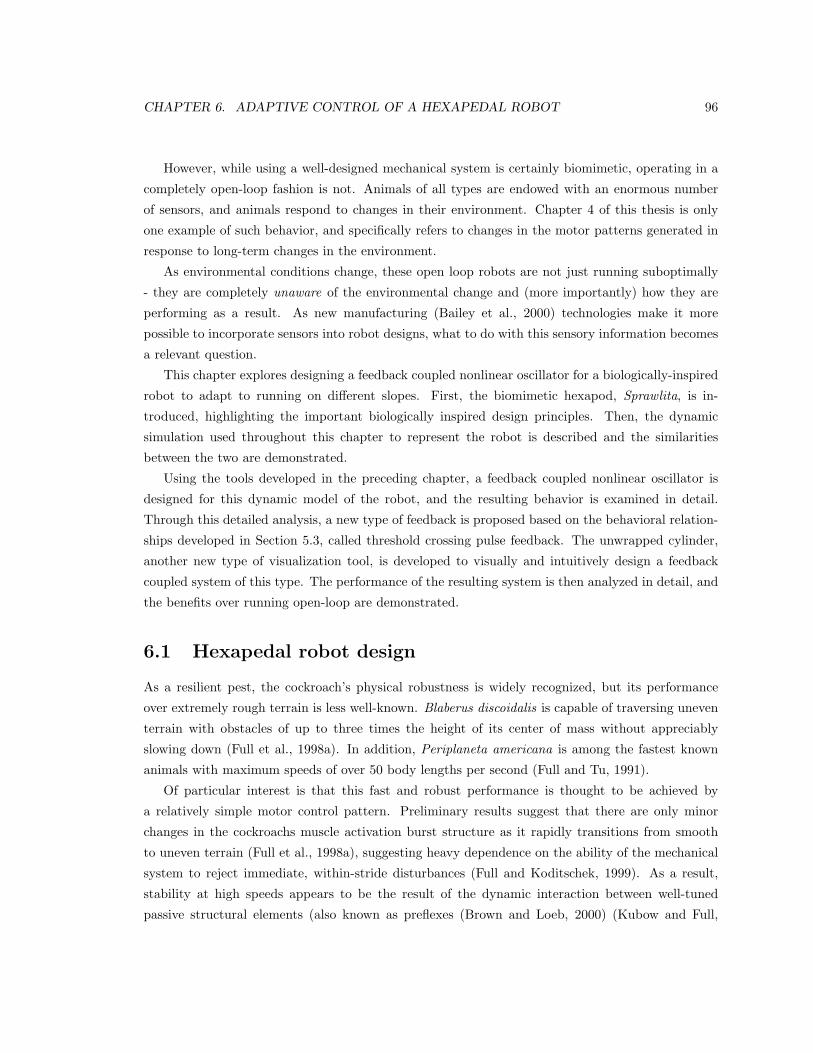
CHAPTER 6. ADAPTIVE CONTROL OF A HEXAPEDAL ROBOT 96
However, while using a well-designed mechanical system is certainly biomimetic, operating in a
completely open-loop fashion is not. Animals of all types are endowed with an enormous number
of sensors, and animals respond to changes in their environment. Chapter 4 of this thesis is only
one example of such behavior, and specifically refers to changes in the motor patterns generated in
response to long-term changes in the environment.
As environmental conditions change, these open loop robots are not just running suboptimally
- they are completely unaware of the environmental change and (more importantly) how they are
performing as a result. As new manufacturing (Bailey et al., 2000) technologies make it more
possible to incorporate sensors into robot designs, what to do with this sensory information becomes
a relevant question.
This chapter explores designing a feedback coupled nonlinear oscillator for a biologically-inspired
robot to adapt to running on different slopes. First, the biomimetic hexapod, Sprawlita, is in-
troduced, highlighting the important biologically inspired design principles. Then, the dynamic
simulation used throughout this chapter to represent the robot is described and the similarities
between the two are demonstrated.
Using the tools developed in the preceding chapter, a feedback coupled nonlinear oscillator is
designed for this dynamic model of the robot, and the resulting behavior is examined in detail.
Through this detailed analysis, a new type of feedback is proposed based on the behavioral relation-
ships developed in Section 5.3, called threshold crossing pulse feedback. The unwrapped cylinder,
another new type of visualization tool, is developed to visually and intuitively design a feedback
coupled system of this type. The performance of the resulting system is then analyzed in detail, and
the benefits over running open-loop are demonstrated.
6.1 Hexapedal robot design
As a resilient pest, the cockroach’s physical robustness is widely recognized, but its performance
over extremely rough terrain is less well-known. Blaberus discoidalis is capable of traversing uneven
terrain with obstacles of up to three times the height of its center of mass without appreciably
slowing down (Full et al., 1998a). In addition, Periplaneta americana is among the fastest known
animals with maximum speeds of over 50 body lengths per second (Full and Tu, 1991).
Of particular interest is that this fast and robust performance is thought to be achieved by
a relatively simple motor control pattern. Preliminary results suggest that there are only minor
changes in the cockroachs muscle activation burst structure as it rapidly transitions from smooth
to uneven terrain (Full et al., 1998a), suggesting heavy dependence on the ability of the mechanical
system to reject immediate, within-stride disturbances (Full and Koditschek, 1999). As a result,
stability at high speeds appears to be the result of the dynamic interaction between well-tuned
passive structural elements (also known as preflexes (Brown and Loeb, 2000) (Kubow and Full,
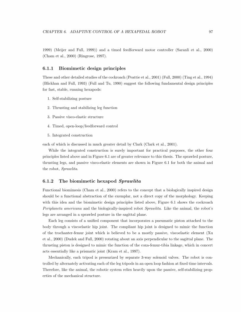
CHAPTER 6. ADAPTIVE CONTROL OF A HEXAPEDAL ROBOT 97
1999) (Meijer and Full, 1999)) and a timed feedforward motor controller (Saranli et al., 2000)
(Cham et al., 2000) (Ringrose, 1997).
6.1.1 Biomimetic design principles
These and other detailed studies of the cockroach (Peattie et al., 2001) (Full, 2000) (Ting et al., 1994)
(Blickhan and Full, 1993) (Full and Tu, 1990) suggest the following fundamental design principles
for fast, stable, running hexapods:
1. Self-stabilizing posture
2. Thrusting and stabilizing leg function
3. Passive visco-elastic structure
4. Timed, open-loop/feedforward control
5. Integrated construction
each of which is discussed in much greater detail by Clark (Clark et al., 2001).
While the integrated construction is surely important for practical purposes, the other four
principles listed above and in Figure 6.1 are of greater relevance to this thesis. The sprawled posture,
thrusting legs, and passive visco-elastic elements are shown in Figure 6.1 for both the animal and
the robot, Sprawlita.
6.1.2 The biomimetic hexapod Sprawlita
Functional biomimesis (Cham et al., 2000) refers to the concept that a biologically inspired design
should be a functional abstraction of the exemplar, not a direct copy of the morphology. Keeping
with this idea and the biomimetic design principles listed above, Figure 6.1 shows the cockroach
Periplaneta americana and the biologically-inspired robot Sprawlita. Like the animal, the robot’s
legs are arranged in a sprawled posture in the sagittal plane.
Each leg consists of a unified component that incorporates a pneumatic piston attached to the
body through a viscoelastic hip joint. The compliant hip joint is designed to mimic the function
of the trochanter-femur joint which is believed to be a mostly passive, viscoelastic element (Xu
et al., 2000) (Dudek and Full, 2000) rotating about an axis perpendicular to the sagittal plane. The
thrusting piston is designed to mimic the function of the coxa-femur-tibia linkage, which in concert
acts essentially like a prismatic joint (Kram et al., 1997).
Mechanically, each tripod is pressurized by separate 3-way solenoid valves. The robot is con-
trolled by alternately activating each of the leg tripods in an open loop fashion at fixed time intervals.
Therefore, like the animal, the robotic system relies heavily upon the passive, self-stabilizing prop-
erties of the mechanical structure.
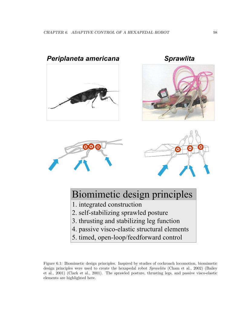
CHAPTER 6. ADAPTIVE CONTROL OF A HEXAPEDAL ROBOT 98Crop special 2.2
Usual crop is top and bottom: 2.3375Left and right: 1.4375
Biomimetic design principles1. integrated construction2. self-stabilizing sprawled posture3. thrusting and stabilizing leg function4. passive visco-elastic structural elements5. timed, open-loop/feedforward control
Periplaneta americana Sprawlita
Periplaneta americana Sprawlita
Fix center of mass symbol
N
Figure 6.1: Biomimetic design principles. Inspired by studies of cockroach locomotion, biomimeticdesign principles were used to create the hexapedal robot Sprawlita (Cham et al., 2002) (Baileyet al., 2001) (Clark et al., 2001). The sprawled posture, thrusting legs, and passive visco-elasticelements are highlighted here.

CHAPTER 6. ADAPTIVE CONTROL OF A HEXAPEDAL ROBOT 99
Despite this simple mechanical arrangement and motor controller, Sprawlita can achieve speeds
of over 3 body lengths per second, or 0.55 m/s, and can overcome hip-height obstacles with little
difficulty. This performance, though humble in light of the cockroach’s, begins to compare to that
seen in nature.
Empirical explorations of the many possible configurations of the robot lead to two relevant
conclusions. First, the range of values which result in stable operation is exceptionally large - even
significant changes in leg angles and stride frequencies result in forward locomotion, an impressive
contrast to the seemingly delicate stability achieved by most bipedal walkers. Despite this large range
of permissible operational values, the performance of the robot suffers if poor choices are made. To
more efficiently explore parameter variations and adaptation schemes, especially in light of changing
environmental conditions, a detailed dynamic model was developed for numerical simulation studies
(Clark, 2004).
6.1.3 ADAMS modeling
The dynamic model developed in ADAMS (MSC.Software Corporation, 2 MacArthur Place, Santa
Ana, CA 92707) by Clark (Clark, 2004) was used for the stride adaptation exploration described in
the remainder of this chapter. Like all other models, the goal of Clark’s detailed dynamic model was
to capture the essential characteristics of Sprawlita’s locomotion as a biomimetic hexapod without
being overly specific. While single degree of freedom hoppers can yield certain insight, essential
characteristics such as sprawled posture and differential leg function cannot be captured by such
simple models.
Shown in Figure 6.2, the ADAMS model developed and verified by Clark (Clark, 2004) captures
the important biomimetic characteristics designed into Sprawlita. The sprawled posture, thrusting
legs, and visco-elastic flexures are specifically designed into the model. Care is taken that the
dynamic properties are descriptive of the ratios present in the real robot and are empirically verified
(Clark, 2004). In addition, practical details such as valve and pneumatic actuation dynamics are
included, giving confidence that trends and adaptation schemes are easily translated to the actual
robot platform.
While many empirical tests were performed, two are reproduced here: measuring ground reaction
forces and slope running performance. Ground reaction forces describe the fundamental interaction
of the robot with the world, and similar ground reaction forces indicate dynamic similarity in running.
While the robot ground reaction forces turn out to be slightly different than those of the cockroach
(Bailey et al., 2001), Figure 6.2 shows that the ADAMS model captures the characteristic ground
reaction forces seen in the robot (Clark, 2004).
In addition to measuring ground reaction forces, the robots were run over a variety of slopes at
different frequencies1. While the performance curves generated are fairly broad, for each robot the1To avoid turning on uphill slopes, the simulation of the robot was constrained to run in a straight line, effected
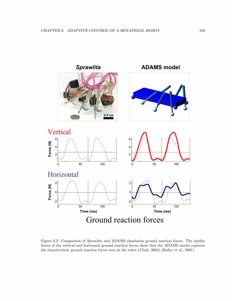
CHAPTER 6. ADAPTIVE CONTROL OF A HEXAPEDAL ROBOT 100
Vertical
2
4
6
-2
0
2
0 50 100
2
4
6
-2
0
2
Time (ms)
Horizontal
Forc
e (N
)Fo
rce
(N)
0 50 100
Time (ms)
0 50 100 0 50 100
Crop special 2.2
Usual crop is top and bottom: 2.3375Left and right: 1.4375
2.5 cm
Sprawlita ADAMS model
Ground reaction forces
Ve
-
Ho
Forc
e (N
)Fo
rce
(N)
Figure 6.2: Comparison of Sprawlita and ADAMS simulation ground reaction forces. The similarforms of the vertical and horizontal ground reaction forces show that the ADAMS model capturesthe characteristic ground reaction forces seen in the robot (Clark, 2004) (Bailey et al., 2001).
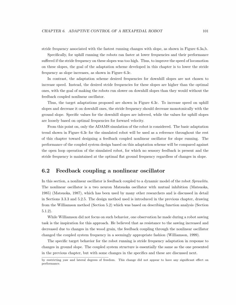
CHAPTER 6. ADAPTIVE CONTROL OF A HEXAPEDAL ROBOT 101
stride frequency associated with the fastest running changes with slope, as shown in Figure 6.3a,b.
Specifically, for uphill running the robots ran faster at lower frequencies and their performance
suffered if the stride frequency on these slopes was too high. Thus, to improve the speed of locomotion
on these slopes, the goal of the adaptation scheme developed in this chapter is to lower the stride
frequency as slope increases, as shown in Figure 6.3c.
In contrast, the adaptation scheme desired frequencies for downhill slopes are not chosen to
increase speed. Instead, the desired stride frequencies for these slopes are higher than the optimal
ones, with the goal of making the robots run slower on downhill slopes than they would without the
feedback coupled nonlinear oscillator.
Thus, the target adaptations proposed are shown in Figure 6.3c. To increase speed on uphill
slopes and decrease it on downhill ones, the stride frequency should decrease monotonically with the
ground slope. Specific values for the downhill slopes are inferred, while the values for uphill slopes
are loosely based on optimal frequencies for forward velocity.
From this point on, only the ADAMS simulation of the robot is considered. The basic adaptation
trend shown in Figure 6.3c for the simulated robot will be used as a reference throughout the rest
of this chapter toward designing a feedback coupled nonlinear oscillator for slope running. The
performance of the coupled system design based on this adaptation scheme will be compared against
the open loop operation of the simulated robot, for which no sensory feedback is present and the
stride frequency is maintained at the optimal flat ground frequency regardless of changes in slope.
6.2 Feedback coupling a nonlinear oscillator
In this section, a nonlinear oscillator is feedback coupled to a dynamic model of the robot Sprawlita.
The nonlinear oscillator is a two neuron Matsuoka oscillator with mutual inhibition (Matsuoka,
1985) (Matsuoka, 1987), which has been used by many other researchers and is discussed in detail
in Sections 3.3.3 and 5.2.5. The design method used is introduced in the previous chapter, drawing
from the Williamson method (Section 5.2) which was based on describing function analysis (Section
5.1.2).
While Williamson did not focus on such behavior, one observation he made during a robot sawing
task is the inspiration for this approach. He believed that as resistance to the sawing increased and
decreased due to changes in the wood grain, the feedback coupling through the nonlinear oscillator
changed the coupled system frequency in a seemingly appropriate fashion (Williamson, 1999).
The specific target behavior for the robot running is stride frequency adaptation in response to
changes in ground slope. The coupled system structure is essentially the same as the one presented
in the previous chapter, but with some changes in the specifics and these are discussed next.
by restricting yaw and lateral degrees of freedom. This change did not appear to have any significant effect onperformance.
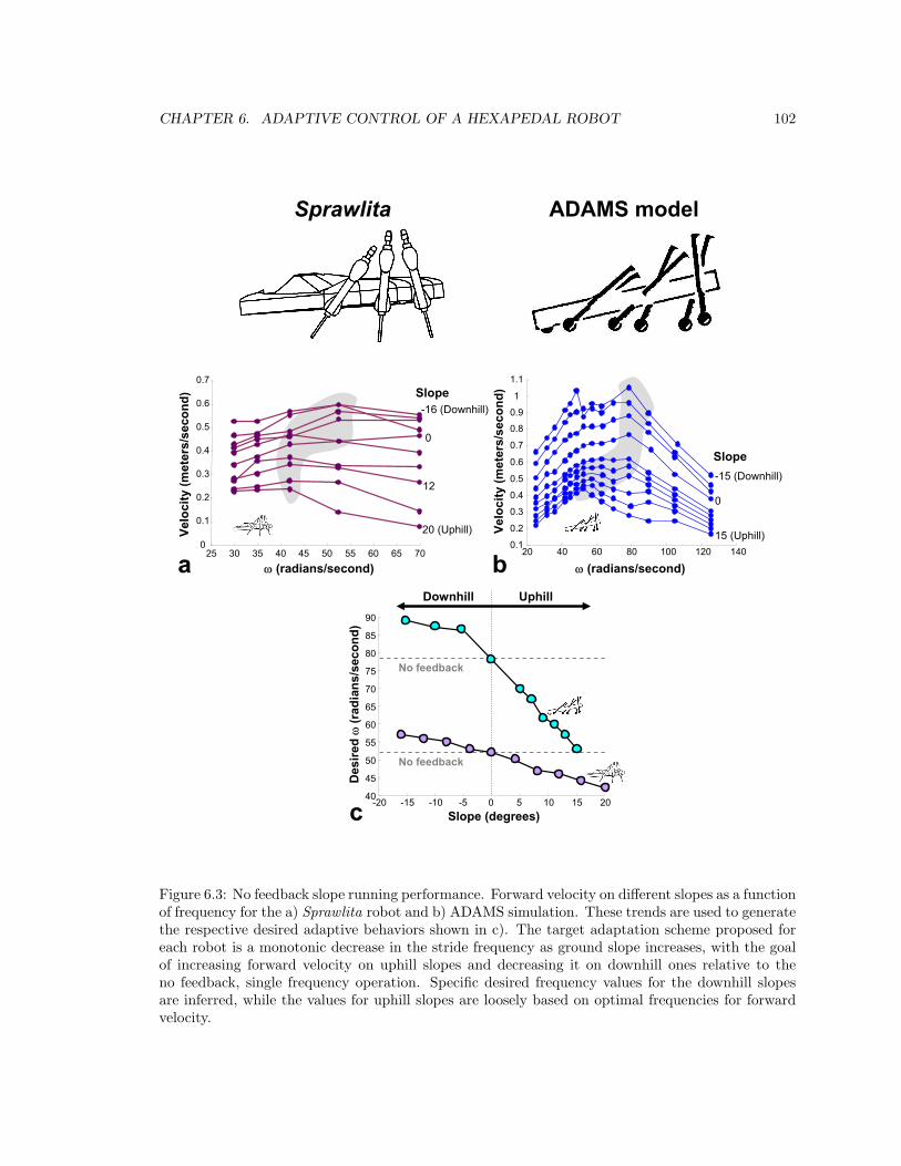
CHAPTER 6. ADAPTIVE CONTROL OF A HEXAPEDAL ROBOT 102
Crop special 2.2
Usual crop is top and bottom: 2.3375Left and right: 1.4375
Sprawlita ADAMS model
25 30 35 40 45 50 55 60 65 700
0.1
0.2
0.3
0.4
0.5
0.6
0.7
-16 (Downhill)
0
12
20 (Uphill)
ω (radians/second)
Velo
city
(met
ers/
seco
nd) Slope
-20 -15 -10 -5 0 5 10 15 2040
45
50
55
60
65
70
75
80
85
90
Des
ired ω
(rad
ians
/sec
ond)
Slope (degrees)
UphillDownhill
Remember to say tThe points of desirAre interpreted, noDirect from velocity
-15 (Downhill)
0
15 (Uphill)
Slope
20 40 60 80 100 120 1400.1
0.2
0.3
0.4
0.5
0.6
0.7
0.8
0.9
1
1.1
Velo
city
(met
ers/
seco
nd)
ω (radians/second)a b
c
No feedback
No feedback
Figure 6.3: No feedback slope running performance. Forward velocity on different slopes as a functionof frequency for the a) Sprawlita robot and b) ADAMS simulation. These trends are used to generatethe respective desired adaptive behaviors shown in c). The target adaptation scheme proposed foreach robot is a monotonic decrease in the stride frequency as ground slope increases, with the goalof increasing forward velocity on uphill slopes and decreasing it on downhill ones relative to theno feedback, single frequency operation. Specific desired frequency values for the downhill slopesare inferred, while the values for uphill slopes are loosely based on optimal frequencies for forwardvelocity.
CHAPTER 6. ADAPTIVE CONTROL OF A HEXAPEDAL ROBOT 103
6.2.1 Nonlinear oscillator coupling details
The main difference between the robot model and the 2nd order mass-spring-damper model discussed
in the previous chapter is the actuation of each system. Previously, the raw output of the nonlinear
oscillator was used as a force applied to the 2nd order system mass. In contrast, the robot is actuated
via two binary pneumatic valves, and a more digital signal is required. Therefore, the output of the
controller is the sign of the nonlinear oscillator output, with a positive value opening one valve and a
negative one opening the other2. Since the valve signal determines the stride frequency of the robot,
the nonlinear oscillator frequency is the same as the stride frequency (as opposed to a harmonic).
As shown in Figure 6.4, the implication for the coupled system design is that controller output
and plant input gains no longer have meaning and are removed. As a digital signal, amplitude does
not have meaning, but a value of +/-1 is used for describing function analysis purposes.
A more subtle implication of such an actuation scheme is that the nonlinear oscillator is implicitly
not responsible for responding to within stride perturbations or suboptimalities. With a more
continuous signal, subtle variations in the shape of the input can correct these, enriching the role
of the nonlinear oscillator but also making it more difficult to understand the specific contribution.
A low-frequency digital signal like the one used here is truly only capable of determining the stride
frequency of the robot, without being able to specify other within stride parameters, such as the
strength of each activation during the course of the stride.
This is important as there are many levels of environmental response, and a basic hierarchy is
listed here (Abbas and Full, 2000) (Full and Koditschek, 1999):
• passive (mechanical feedback)
• reflexes (lowest level sensor-based response)
• Motor pattern generator adaptation (change in the feedforward signal)
• High level navigation-type control (vision-based, volitional)
Passive mechanical feedback certainly plays an important role in the locomotion, as discussed in
Section 6.1. However, for this example, there are no reflexes or high-level inputs - the only sensor-
based response comes from the feedback coupled nonlinear oscillator, acting through changes in the
feedforward motor pattern it generates. Thus, the changes in actuation that occur are solely due to
the nonlinear oscillator contributions. This is an important point, as many other robotic systems
using similar feedback coupled nonlinear oscillators have multiple other sensory-based mechanisms
also in place, and the relative contributions of each individual component are difficult to distinguish
(Fukuoka et al., 2003) (Kimura et al., 1999) (Zhang et al., 2003) (Lewis and Bekey, 2002).2The sign function used incorporates hysteresis, as the valve switch only occurs once the nonlinear oscillator output
actually crosses zero. This is an important consideration as the output of the oscillator can be maintained at zero fora small, but significant amount of time for each cycle (as shown in Figure 6.12), and a way of establishing symmetricvalve activation is necessary.
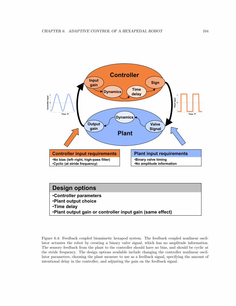
CHAPTER 6. ADAPTIVE CONTROL OF A HEXAPEDAL ROBOT 104
•Binary valve timing•No amplitude information
•No bias (left–right, high-pass filter)•Cyclic (at stride frequency)
Crop special 2.2
Usual crop is top and bottom: 2.3375Left and right: 1.4375
SquaNonlLeft-Cycli
Plan
t inp
ut
0
+
-
•Controller parameters•Plant output choice•Time delay•Plant output gain or controller input gain (same effect)
SignInputgain
Outputgain
ValveSignal
Dynamics
Controller
Dynamics Timedelay
Controller input requirements Plant input requirements
List corresponding sections?
Time
Con
trol
ler I
nput
0
+
-
Time
Plan
t inp
ut
0
+
-
Plant
•Controller parameters•Plant output choice•Time delay•Plant output gain or controller input gain (same effect)
Design options
Figure 6.4: Feedback coupled biomimetic hexapod system. The feedback coupled nonlinear oscil-lator actuates the robot by creating a binary valve signal, which has no amplitude information.The sensory feedback from the plant to the controller should have no bias, and should be cyclic atthe stride frequency. The design options available include changing the controller nonlinear oscil-lator parameters, choosing the plant measure to use as a feedback signal, specifying the amount ofintentional delay in the controller, and adjusting the gain on the feedback signal.
CHAPTER 6. ADAPTIVE CONTROL OF A HEXAPEDAL ROBOT 105
On the other side of the coupled system, the communication signal between the plant and the
controller has similar requirements as the 2nd order mass-spring-damper system. As it is an input to
the oscillatory system, the input should not have any bias, or steady state component. In practice,
this can be achieved by a high-pass filter. In this example though, the bias is removed by using the
difference between contralateral components, specifically left-right.
Additionally, since the output of the nonlinear oscillator is used to determine the stride frequency
of the robot, the output of the plant should be cyclic at the stride frequency. In general, a well-tuned
feedback coupled nonlinear oscillator can be thought of as entrained to the natural dynamics of the
plant, and as such, the frequencies should not be harmonics of one another. It may be possible
to create such a coupled system that gives the behavior desired, but this is not considered in this
thesis. One example of a feedback signal that is a harmonic of the stride frequency is the fore-aft
acceleration, as it varies at twice the frequency of the stride. This is not a statement about the
general quality of such a feedback signal, but instead a consequence of this particular interpretation
of the nonlinear oscillator output into a valve actuation signal. Other interpretations will have
different feedback requirements.
6.2.2 Feedback coupled nonlinear oscillator design
Even with the removal of the controller output and plant input gains as discussed above, there are
still a large number of tunable parameters available for the design of the coupled nonlinear oscillator.
In addition to the choice of feedback from the plant, all of the dynamic parameters of the nonlinear
oscillator are available for tuning.
Choice of feedback
Other than the requirements mentioned above, the initial choice of feedback from the plant to
begin with is somewhat arbitrary. The initial choice made here was the difference in the rear leg
extensions (left-right), guided by the general belief that the front legs are stabilizing, the middle
legs are supportive, and the rear legs are forward velocity thrusters (Full, 2000). Using the difference
in the rear leg extensions fits the requirements listed, as it is an oscillatory signal with zero bias,
with a rate on the order of the stride frequency.
As discussed in section 5.2.3, the plant output and controller input feedback gains are redundant,
and the plant output gain is the only one considered here. Initially, this gain is chosen to make the
amplitude of the feedback signal close to one, for convenience in comparing with the signals from
the previous example in Chapter 5. As the maximum leg extensions are 0.020 meters, the amplitude
of the gain was chosen to be 50.0. As the positive feedback gain plant representation needed to
be rotated by 180◦ to intersect the controller representation, the gain was negated, resulting in a
feedback gain of −50.0.

CHAPTER 6. ADAPTIVE CONTROL OF A HEXAPEDAL ROBOT 106
Choosing basic nonlinear oscillator parameters
Introduced in Section 3.3.3 and discussed further in Section 5.2.5, the two neuron Matsuoka oscillator
with mutual inhibition (Matsuoka, 1985) (Matsuoka, 1987) used for the controller is described by
Equations 6.1-6.9:
x1 =1τ1
(c− x1 − βv1 − γ[x2]+ −∑
j
hj [gj ]+) (6.1)
v1 =1τ2
([x1]+ − v1) (6.2)
x2 =1τ1
(c− x2 − βv2 − γ[x1]+ −∑
j
hj [gj ]−) (6.3)
v2 =1τ2
([x2]+ − v2) (6.4)
[xi]+ = max(xi, 0) (6.5)
[gj ]+ = max(gj , 0) (6.6)
[gj ]− = max(−gj , 0) = −min(gj , 0) (6.7)
yi = [xi]+ (6.8)
y = y1 − y2 (6.9)
As discussed in section 5.2.5, however, none of tunable parameters are effective for tuning once the
self-sustained limit cycle frequency of the nonlinear oscillator has been chosen, since they will affect
that frequency.
As suggested in Table 5.1, τ1 is used to set the self-sustained limit cycle frequency of the nonlinear
oscillator. For the set of values for τ2:τ1, β, γ, and c listed in Table 5.1, τ1=0.112T , where T is
the period of the self sustained limit cycle period. To make the system robust to complete sensor
failure, this frequency should be set to the optimal stride frequency for flat ground. In this case,
this frequency is 78.5 radians/second, which corresponds to a period of T=0.08 seconds and results
in a τ1 value of 0.009.
The final remaining design parameter is the intentional time delay of the controller output, as
introduced in section 5.3.4. This should be thought of as a fine-tuning parameter, and is left at 0.0
seconds until the visualization is developed. Once at that stage of the design, the time delay can be
used to select plant controller intersections with a great deal of resolution.
Three dimensional visualization of the preliminary design
At this point, the visualization and design tools developed in the previous chapter in section 5.3 can
be used to predict the coupled system behavior. Using the intersection of the plant and controller
surfaces shown in Figure 6.5a, a solution trend can be visualized.
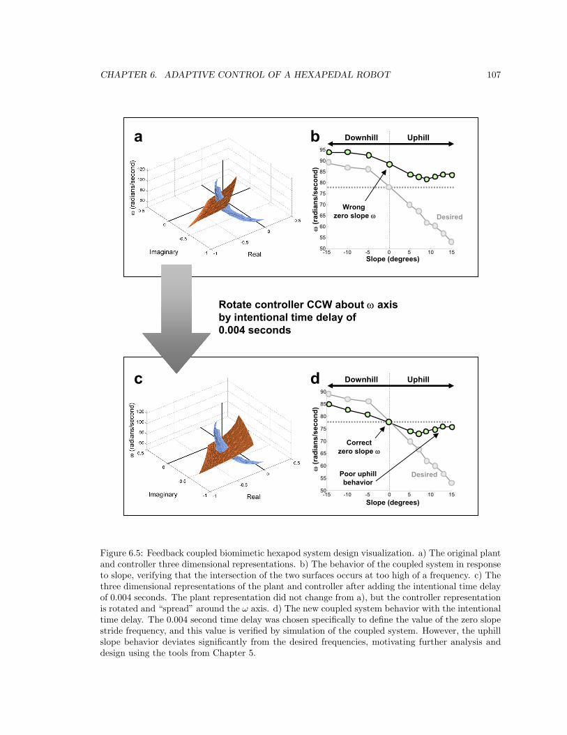
CHAPTER 6. ADAPTIVE CONTROL OF A HEXAPEDAL ROBOT 107Crop special 2.2
Usual crop is top and bottom: 2.3375Left and right: 1.4375
SlopWith
In b
SWit
BAb
Rotate controller CCW about ω axis by intentional time delay of 0.004 seconds
-15 -10 -5 0 5 10 1550
55
60
65
70
75
80
85
90
95
Slope (degrees)
-15 -10 -5 0 5 10 1550
55
60
65
70
75
80
85
90
ω(r
adia
ns/s
econ
d)
Desired
UphillDownhill
ω(r
adia
ns/s
econ
d)
Slope (degrees)
UphillDownhill
DesiredPoor uphillbehavior
Correctzero slope ω
Wrong zero slope ω
a
c
b
d
Figure 6.5: Feedback coupled biomimetic hexapod system design visualization. a) The original plantand controller three dimensional representations. b) The behavior of the coupled system in responseto slope, verifying that the intersection of the two surfaces occurs at too high of a frequency. c) Thethree dimensional representations of the plant and controller after adding the intentional time delayof 0.004 seconds. The plant representation did not change from a), but the controller representationis rotated and “spread” around the ω axis. d) The new coupled system behavior with the intentionaltime delay. The 0.004 second time delay was chosen specifically to define the value of the zero slopestride frequency, and this value is verified by simulation of the coupled system. However, the uphillslope behavior deviates significantly from the desired frequencies, motivating further analysis anddesign using the tools from Chapter 5.
CHAPTER 6. ADAPTIVE CONTROL OF A HEXAPEDAL ROBOT 108
Using commonly available three dimensional graphical packages (such as Matlab), animated
rotation of the three dimensional visualization reveals that the intersection occurs at too high of an
ω, and this is verified by simulation of the coupled system. As shown in the ω versus slope behavior
plot of Figure 6.5b, the zero slope frequency of the coupled system is close to 90 radians/second,
much higher than the optimal stride frequency of 78.5 radians/second. Additionally, the three
dimensional visualization makes it possible to see that this intersection frequency can be lowered by
rotating the controller counterclockwise (CCW) about the ω axis.
Choosing the intentional time delay to design zero slope intersection
While usually avoided in control designs, intentionally inserting a time delay can actually be ben-
eficial in this case. As developed in Section 5.3.4, the intentional time delay rotates the controller
CCW with a fine degree of resolution.
As the controller shape can be regenerated rather quickly (5 minutes on a 3 GHz Pentium 4 PC),
an iterative method is employed to get the intersection of choice in the visualization, as shown in
Figure 6.5c. This result is verified through simulation and the coupled system zero slope frequency
is very near the desired 78.5 radians/second, as shown in Figure 6.5d.
Behavior analysis
With the zero slope intersection at the desired frequency, attention is turned to the behavior as the
robot encounters slopes of different inclinations. On downhill slopes, the robot does increase the
stride frequency, decreasing the forward velocity relative to the no feedback case.
On uphill slopes, though, the behavioral trend deviates from that which is desired. Instead of
continuing to decrease the stride frequency as the slope of the ground increases, the feedback coupling
only minimally changes the stride frequency from the open-loop, no feedback value. This deviation
from the desired behavior can be seen in Figure 6.5d, as the coupled system stride frequency stays
close to the zero slope frequency instead of dropping significantly. In fact, the stride frequency even
begins to increase again as the slope increases, opposite of the desired effect.
Unfortunately, this effect is not isolated to the difference in rear leg extensions. All the other types
of possible feedback checked (leg extensions, velocities, accelerations and lateral body accelerations)
demonstrated similar trends. An interesting phenomenon, the details of the rear leg extension
feedback are examined more closely in the following section using the tools developed in Chapter 5,
and the resulting insights are used to slightly modify this measure into a more appropriate feedback
signal.
CHAPTER 6. ADAPTIVE CONTROL OF A HEXAPEDAL ROBOT 109
6.3 Phase relationship driven feedback coupled nonlinear os-
cillator design
This section examines the feedback used in the feedback coupled nonlinear oscillator design as
described in the previous section. While the design tools developed in Chapter 5 were sufficient to
specify the zero slope operation frequency, the associated behavior was significantly different than
the desired trend. The ω contour analysis from Section 5.3.2 is used to closely examine the phase-
based reasons for this behavior, and the fundamental source is revealed by an even more in-depth
look. Ultimately, this analysis leads to a characteristically different form of the same feedback, one
that is more appropriate for the adaptation desired.
6.3.1 ω contour and phase analysis of coupled system
While the three dimensional visualization is a more intuitive representation of the coupled system
solution space, ω contour analysis is more appropriate in two dimensions. Figure 6.6a shows a
closeup of the ω contours of the plant and the controller.
Using the methodology developed in section 5.3.2 and shown in Figure 5.14, to get the desired
behavioral trends the plant needs to be rotated counterclockwise (CCW) relative to the controller.
In terms of phase, a CCW rotation corresponds to the phase of the plant decreasing as the slope
increases (using the convention that downhill slopes are negative, and remembering that CCW
rotations on the phase plane correspond to increasing phase). As the ω contours of the controller
are essentially radial, the plant ω contours can be compared directly to a true radial line, which
represents a constant phase as shown in Figure 6.6a.
For downhill slopes, the plant is indeed rotated CCW relative to the constant phase radial line,
and the desired behavior is achieved. From -15 to +5 degrees of slope, the plant phase decreases.
Correspondingly, the coupled system stride frequency decreases monotonically as the robot runs over
this range of slopes.
However, the uphill portion of the plant ω contours are essentially radial, following the line of
constant phase, as shown in Figure 6.6a. Because the phase does not decrease with increasing slope
in the range from +5 to +15 degrees, the coupled system stride frequency also does not change
significantly. In fact, the slight clockwise (CW) rotation of the phase relative to the constant phase
line results in the frequency actually increasing from +11 to +15 degrees.
Correlation to a 2nd order system
To draw an analogy, the two regions can be compared to the phase relationships exhibited by a
2nd order spring-mass-damper system above and below resonance, as shown in Figure 6.6b,c. This

CHAPTER 6. ADAPTIVE CONTROL OF A HEXAPEDAL ROBOT 110
-0.4
-0.35
Crop special 2.2
Usual crop is top and bottom: 2.3375Left and right: 1.4375
dial,ncyses
SP
Phase is impoThis plot is ofof the plant a
-1.5 -1 -0.5 0 0.5 1 1.5 2
-2.5
-2
-1.5
-1
-0.5
0
Real
Imag
inar
y
0.1 1 100
0.5
1
1.5
2
2.5
3
-200
-150
-100
-50
0
2D - 1 pt and .5pt
Res
onan
ce
Below
Above
ζ+
ω+
Gai
n
Frequency (Hz)
Phas
e (d
egre
es)
0.1 1 10
ζ+ζ+
ζ+R
eson
ance
-0.5 -0.45 -0.4 -0.35 -0.3 -0.25 -0.2 -0.15
-0.6
-0.55
-0.5
-0.45
15
0
-15
Real
Imag
inar
y
Const
ant
Phas
e
ControllerCoupled System
Plant
b
a
c
-15
-1 -0.8 -0.6 -0.4 -0.2 0 0.2-1
-0.9
-0.8
-0.7
-0.6
-0.5
-0.4
-0.3
-0.2
-0.1
0
0.1
0
Real
Imag
inar
y 15
0
Constant
Phase
-15
-1 -0.8 -0.6 - -0.2 0 0.2-1
-0.9
-0.8
-0.7
-0.6
-0.5
-0.4
-0.3
-0.2
-0.1
0
0.1
0
Real
Imag
inar
y 15
0
Constant
Phase
A+
ω+ω+
ω+ω+A+
Slope+
These + things make it ugly – should I remove?
Figure 6.6: ω contour analysis of the feedback coupled biomimetic hexapod design. a) A closeupof the two dimensional visualization of the plant and controller representations, highlighting theω contours. Given the relationships established in Section 5.3.2, the desired behavioral trend ofdecreasing stride frequency as slope increases dictates that the ω contours of the plant need to berotated counterclockwise (CCW) relative to those of the controller. This is the case for downhill(negative) slopes, but not for the uphill ones, corresponding to the observed deviation from thedesired behavior. b) The ω contours of a 2nd order spring-mass-damper system (Equation 6.10)broken into regions of above, at, and below resonance, for correlation with the ω contours of therobot plant (see text). c) Frequency response plot of the 2nd order system. The 2nd order systemparameters are m=1 and k=1, and therefore ωn=1 (b varies with ζ). A+ refers to increasing forcingfunction amplitudes, ω+ refers to increasing forcing function and valve frequencies, Slope+ refersto increasing ground slopes, and ζ+ refers to increasing damping ratios.
CHAPTER 6. ADAPTIVE CONTROL OF A HEXAPEDAL ROBOT 111
second order system is described by Equation 6.10:
mx + bx + kx = FInput (6.10)
where the mass m is 1.0 kilogram and the stiffness k is 1.0 Newton/meter, resulting in a natural
frequency ωn of 1.0 radian/second. The damping coefficient, b, is specified by the damping ratio
ζ. As before in Section 5.3.1, a general connection is made between the damping in this 2nd order
system and the slope of the robot running on a slope for comparison purposes. An ω contour
represents the changing phase of these systems as they are forced at a constant frequency.
When such a 2nd order system is forced at resonance, the phase relationship between the input
and the output is always −90◦, regardless of the amount of damping. In other words, if the input
to the system is held at this fixed frequency, the phase does not change, even as damping increases,
and the ω contour is a vertical line as shown in Figure 6.6b.
Below resonance, as the damping is increased and the forcing frequency is held constant, the
phase decreases (becomes more negative) as can be seen in the left side of the Bode plot in Figure
6.6c. This effect causes the 2nd order system ω contour to rotate CCW as the damping is increased,
as shown in Figure 6.6b. This is the same effect that is seen with the plant in the slope ranges from
-15 to +5 degrees, resulting in the desired behavior.
In contrast, above resonance the phase of the second order system increases as the amount of
damping is increased and the forcing frequency is held constant. This is demonstrated in the right
side of the Bode plot in Figure 6.6c, and the corresponding CW rotation of the ω contour is seen
in Figure 6.6b. As predicted, this generates the opposite behavioral trend which is shown by the
coupled system behavior in the slope range from +5 to +15 degrees.
In summary, to get the behavior desired, the plant phase needs to monotonically decrease as
the slope increases. This is equivalent to saying that if the slope increasing is represented by the
damping in a 2nd order system, the behavior needs to mimic that of such a system below resonance.
In other words, as the damping (or slope) increases, the phase needs to decrease.
While this correlation makes it easier to understand the implications of the plant phase for
the coupled system, it only leads to conclusions about what type of plant phase is needed for the
behavioral trends desired. Only an in-depth analysis of the reasons behind this phasing present may
yield answers about how to actually generate the phase required.
6.3.2 Detailed feedback analysis
It is somewhat surprising that the relative phase between the valve actuation and the leg extension
does not decrease as the slope of the ground increases. As the robot climbs progressively steeper
slopes, it should be harder for the legs to extend each time, which leads one to think that the phase
should monotonically become more negative, as is desired. However, the trends above show this is
CHAPTER 6. ADAPTIVE CONTROL OF A HEXAPEDAL ROBOT 112
not the case.
Figure 6.7b shows the left and right rear leg extension during downhill, flat, and uphill running.
Above it, Figure 6.7a shows the feedback discussed above, the difference in rear leg extension (left-
right). In each frame of the entire figure, the phase is relative to the valve actuation signal, which
is exactly the same for each case.
Surprisingly, the significant phase shift observed for downhill running is not a direct result of the
leg being easier to extend (than on flat ground). The phase shift is actually a result of the limited
leg stroke, as the robot piston stroke length is only 0.020 meters. After the maximum extension
is reached, the leg maintains this length and the foot is dragged along on the ground. This is not
unexpected, as some dragging occurs on flat ground, a phenomenon that is well documented by
Bailey (Bailey et al., 2001). Interestingly, it is only the slight nonlinearity induced by this dragging
that causes the phase to be more negative on this slope than it would be on flat ground.
Surprising in perhaps a different way is that there is almost no phase shift in the feedback signal
going from flat ground to uphill. Going uphill, the rear legs extend more slowly, but the peak
extension at this inclination is at the same phase as the peak extension on flat ground, resulting in
a negligible phase shift. The legs do not extend to their full length as they do on flat ground, but
this only causes a change in the feedback amplitude, not phase. As the controller ω contours are
essentially radial, this in itself does not produce any change in the coupled system frequency.
Consequently, it is surprising that any stride frequency change occurs on downhill slopes and
the feedback signal is fundamentally insufficient to produce the behavior desired on uphill slopes.
However, with this new understanding of the basic behavior, a new feedback signal is developed that
generates the desired phase relationships.
6.3.3 Threshold crossing pulse feedback
While the phase of the extension of each leg does not change significantly with slope, the rate at
which the leg extends does change. This is an intuitive result, since the legs essentially encounter
more resistance as the slope of the ground increases. This changing extension rate can be seen clearly
by looking at when the leg extensions cross a threshold, as shown in Figure 6.7b. As the slope of
the ground increases, the individual leg extensions cross this threshold at progressively later times.
Given that this is essentially the phase relationship that the feedback signal needs to have, it
makes sense to convert this threshold crossing into a usable feedback signal. Generating a positive
pulse for a fixed amount of time after a 0.010 meter extension threshold has been reached produces
the signal shown in Figure 6.7c. For this signal, left leg extension threshold crossings are represented
by positive bursts and right leg crossings are represented by negative ones. The pulse time in either
direction was selected to be 0.01 seconds, but could have been any value up to one half the minimum
expected stride period (to keep the signals from overlapping).
Like the binary controller output that drives the robot valves, this signal only contains timing
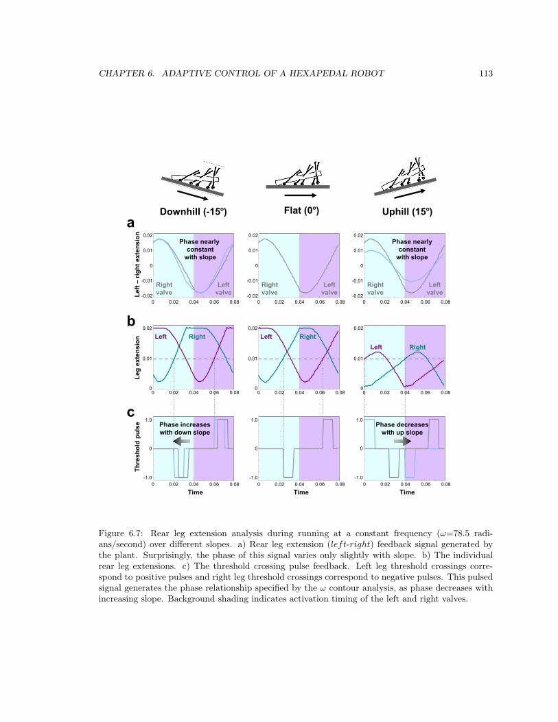
CHAPTER 6. ADAPTIVE CONTROL OF A HEXAPEDAL ROBOT 113
Crop special 2.2
Usual crop is top and bottom: 2.3375Left and right: 1.4375
d)
Downhill (-15o)
legs
Use 2And uFor dPlot jLabe
Uses -15, 0All at
0.01
0.02
0 0.02 0.04 0.06 0.08-0.02
-0.01
0
0.01
0.02
Phase increaseswith down slope
Phase decreaseswith up slope
Phase nearly constant
with slope
Phase nearlyconstant
with slope
Right RightRight
Left LeftLeft
Time
Left
–rig
ht e
xten
sion
-0.02
-0.01
0
0.01
0.02
-0.02
-0.01
0
0.01
0.02
0 0.02 0.04 0.06 0.08 0 0.02 0.04 0.06 0.08
0
Leg
exte
nsio
n
0.01
0.02
0
0.01
0.02
00 0.02 0.04 0.06 0.08 0 0.02 0.04 0.06 0.08 0 0.02 0.04 0.06 0.08
0
1.0
-1.0
0
1.0
-1.0
0
1.0
-1.00 0.02 0.04 0.06 0.08 0 0.02 0.04 0.06 0.08 0 0.02 0.04 0.06 0.08
Time Time
Thre
shol
d pu
lse
Time
Flat (0o) Uphill (15o)a
b
c
Phase dewith up
Is the sameThat Phase la
(sin(phase)=si, ie phase lag beco
But phase becom
Rightvalve
Leftvalve
Rightvalve
Leftvalve
Rightvalve
Leftvalve
Figure 6.7: Rear leg extension analysis during running at a constant frequency (ω=78.5 radi-ans/second) over different slopes. a) Rear leg extension (left-right) feedback signal generated bythe plant. Surprisingly, the phase of this signal varies only slightly with slope. b) The individualrear leg extensions. c) The threshold crossing pulse feedback. Left leg threshold crossings corre-spond to positive pulses and right leg threshold crossings correspond to negative pulses. This pulsedsignal generates the phase relationship specified by the ω contour analysis, as phase decreases withincreasing slope. Background shading indicates activation timing of the left and right valves.
CHAPTER 6. ADAPTIVE CONTROL OF A HEXAPEDAL ROBOT 114
information. An artificial amplitude of one is assigned for reference purposes, but this is where the
similarity between the two signals ends. As shown in the next section, the gains by which this signal
is multiplied do play an important role, as the amplitude of the signal that drives the nonlinear
oscillator affects the coupled system performance.
6.4 Designing a pulse feedback coupled nonlinear oscillator
Designing a pulse feedback coupled nonlinear oscillator is the same in principle as the preceding
nonlinear oscillator design methods presented and used in this thesis. The plant and controller
components are separated and integrated independently, yielding two surfaces in three dimensional
space. The intersection of these surfaces in space is the solution of the coupled system, and defines
the behavior over a set of changing conditions (in this case, slope).
Where designing a pulse feedback coupled nonlinear oscillator differs is in how the surfaces
are generated using the describing function analysis tools. The describing function analysis is an
approximate method, and one of the (many) assumptions is that the fundamental frequency is
descriptive of the signal, and the higher frequency harmonics are negligible (Slotine and Li, 1991). As
the signals analyzed become less sinusoidal, this assumption begins to be violated and the predictive
accuracy of the method is degraded.
In Section 6.2.1, it was noted that a square wave was used to represent the binary valve signal
controller output, a waveform which contains significant higher frequency harmonics. This did not
affect the predictive ability of the method as used in Section 6.2 because the same square wave
signal was used to drive the robot (as opposed to driving the robot with a sinusoidal waveform,
which presumably would have yielded less accurate coupled system solution predictions). Therefore,
the assumptions of the describing function analysis were somewhat violated, but the predictive
accuracy of the solution was maintained because the waveform was known and was used as an input
to the plant.
However, given the new type of feedback, the describing function analysis assumptions no longer
hold for either signal. While this may seemingly cause problems, it actually makes the design easier,
and leads to the development of another design visualization tool.
6.4.1 Alternative to the describing function analysis
While seemingly simple, the pulsed signal shown in Figures 6.7 and 6.8 contains a large number
of frequencies, with significant ones well above the fundamental frequency. The describing function
analysis allows for nonlinear signals, but one of the core assumptions that the fundamental frequency
well describes the signal is violated. In other words, system should act like a low-pass filter in that
the amplitudes of the higher frequency components are significantly reduced (Slotine and Li, 1991)
and this is not the case for the pulse feedback signal.
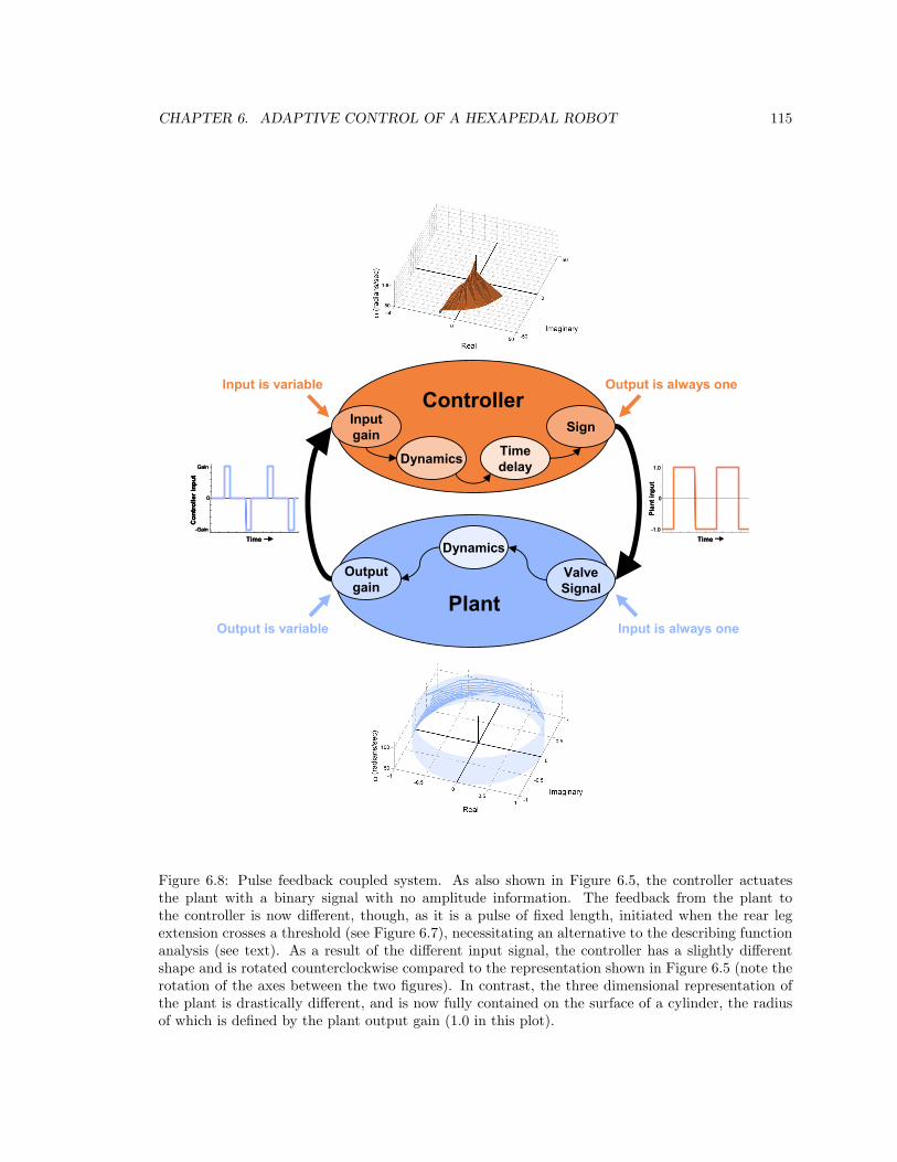
CHAPTER 6. ADAPTIVE CONTROL OF A HEXAPEDAL ROBOT 115
SignInputgain
Outputgain
ValveSignal
Dynamics
Controller
Dynamics Timedelay
Output is always one
Input is always oneOutput is variable
Input is variable
Time
Con
trol
ler i
nput
0
Gain
-Gain
Time
Con
trol
ler i
nput
0
Gain
-Gain
Con
trol
ler i
nput
0
Gain
-Gain
Time
Plan
t inp
ut
0
1.0
-1.0
Time
Plan
t inp
ut
0
1.0
-1.0
Plant
Figure 6.8: Pulse feedback coupled system. As also shown in Figure 6.5, the controller actuatesthe plant with a binary signal with no amplitude information. The feedback from the plant tothe controller is now different, though, as it is a pulse of fixed length, initiated when the rear legextension crosses a threshold (see Figure 6.7), necessitating an alternative to the describing functionanalysis (see text). As a result of the different input signal, the controller has a slightly differentshape and is rotated counterclockwise compared to the representation shown in Figure 6.5 (note therotation of the axes between the two figures). In contrast, the three dimensional representation ofthe plant is drastically different, and is now fully contained on the surface of a cylinder, the radiusof which is defined by the plant output gain (1.0 in this plot).
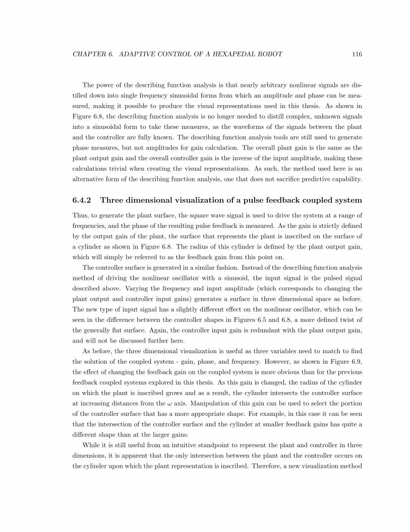
CHAPTER 6. ADAPTIVE CONTROL OF A HEXAPEDAL ROBOT 116
The power of the describing function analysis is that nearly arbitrary nonlinear signals are dis-
tilled down into single frequency sinusoidal forms from which an amplitude and phase can be mea-
sured, making it possible to produce the visual representations used in this thesis. As shown in
Figure 6.8, the describing function analysis is no longer needed to distill complex, unknown signals
into a sinusoidal form to take these measures, as the waveforms of the signals between the plant
and the controller are fully known. The describing function analysis tools are still used to generate
phase measures, but not amplitudes for gain calculation. The overall plant gain is the same as the
plant output gain and the overall controller gain is the inverse of the input amplitude, making these
calculations trivial when creating the visual representations. As such, the method used here is an
alternative form of the describing function analysis, one that does not sacrifice predictive capability.
6.4.2 Three dimensional visualization of a pulse feedback coupled system
Thus, to generate the plant surface, the square wave signal is used to drive the system at a range of
frequencies, and the phase of the resulting pulse feedback is measured. As the gain is strictly defined
by the output gain of the plant, the surface that represents the plant is inscribed on the surface of
a cylinder as shown in Figure 6.8. The radius of this cylinder is defined by the plant output gain,
which will simply be referred to as the feedback gain from this point on.
The controller surface is generated in a similar fashion. Instead of the describing function analysis
method of driving the nonlinear oscillator with a sinusoid, the input signal is the pulsed signal
described above. Varying the frequency and input amplitude (which corresponds to changing the
plant output and controller input gains) generates a surface in three dimensional space as before.
The new type of input signal has a slightly different effect on the nonlinear oscillator, which can be
seen in the difference between the controller shapes in Figures 6.5 and 6.8, a more defined twist of
the generally flat surface. Again, the controller input gain is redundant with the plant output gain,
and will not be discussed further here.
As before, the three dimensional visualization is useful as three variables need to match to find
the solution of the coupled system - gain, phase, and frequency. However, as shown in Figure 6.9,
the effect of changing the feedback gain on the coupled system is more obvious than for the previous
feedback coupled systems explored in this thesis. As this gain is changed, the radius of the cylinder
on which the plant is inscribed grows and as a result, the cylinder intersects the controller surface
at increasing distances from the ω axis. Manipulation of this gain can be used to select the portion
of the controller surface that has a more appropriate shape. For example, in this case it can be seen
that the intersection of the controller surface and the cylinder at smaller feedback gains has quite a
different shape than at the larger gains.
While it is still useful from an intuitive standpoint to represent the plant and controller in three
dimensions, it is apparent that the only intersection between the plant and the controller occurs on
the cylinder upon which the plant representation is inscribed. Therefore, a new visualization method
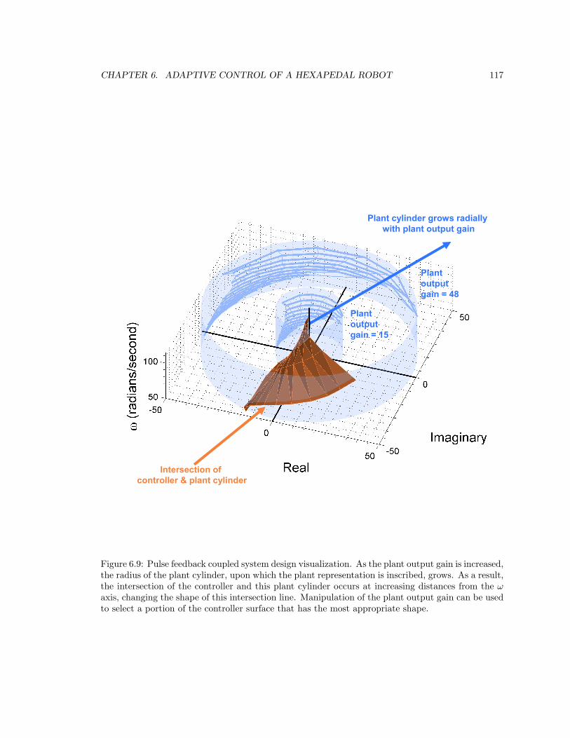
CHAPTER 6. ADAPTIVE CONTROL OF A HEXAPEDAL ROBOT 117
Crop special 2.2
Plantoutputgain = 48
Plantoutputgain = 15
Plant cylinder grows radiallywith plant output gain
Intersection of controller & plant cylinder
Figure 6.9: Pulse feedback coupled system design visualization. As the plant output gain is increased,the radius of the plant cylinder, upon which the plant representation is inscribed, grows. As a result,the intersection of the controller and this plant cylinder occurs at increasing distances from the ωaxis, changing the shape of this intersection line. Manipulation of the plant output gain can be usedto select a portion of the controller surface that has the most appropriate shape.
CHAPTER 6. ADAPTIVE CONTROL OF A HEXAPEDAL ROBOT 118
is presented in which this “phase cylinder” is unwrapped and the gain dimension is collapsed.
6.4.3 Unwrapped phase cylinder visualization method
As shown in Figure 6.10a, this visualization collapses the three dimensional representation of the
plant and the controller by unwrapping the phase cylinder and representing it two dimensionally. In
this two dimensional representation, phase is plotted on the horizontal axis, while ω is plotted on
the vertical axis.
As shown in Figure 6.10b, there are many nearly vertical lines representing running across dif-
ferent slopes for the robot plant. The controller is also represented by a number of nearly vertical
lines, describing the intersection of the plant cylinder and the controller surface at different levels of
feedback gain as described above. As such, these lines are labeled with the corresponding feedback
gain.
As before, the solution of the coupled system is where the plant and controller representations
intersect, representing that the gain, phase, and frequency of each component are equal. The gains
are the easiest to match, as they are abstracted away from the representation, except for selecting
the appropriate controller line. After this selection, only the phase and frequencies need to match,
and the solution is easily visualized.
With the coupled system as is, the intersection is predicted only for a feedback gain of 1.0. While
the predicted solution line from Figure 6.10b would yield the desired behavioral trend of decreasing
stride frequency with increasing slope, the range of solution frequencies are much lower than those
which are desired. The design tools developed earlier are still usable here, and the effect they have
on the representations in this visualization are even easier to understand.
6.4.4 Phase shifting by negation and intentional time delay
The parameters of the nonlinear oscillator are not re-examined, as the controller still functions in
fundamentally the same way in the pulsed and non-pulsed feedback configurations. Therefore, as
before, once the feedback from the plant has been chosen, the most effective design tools for tuning
the intersection are the gain selection (including negation) and intentional time delays. As the phase
cylinder is unwrapped and represented on a linear axis, the phase change induced rotations about
the ω axis in the three dimensional visualization now correspond to shifts of the representations on
the phase axis.
Accordingly, negating the feedback results in the plant being shifted 180◦ on the phase axis, as
shown in Figure 6.10c. This shift does not alter the shape of the plant at all, but brings the shapes
of the plant and controller closer together. Unfortunately, none of the controller lines even intersect
the zero slope plant line, indicating that the 180◦ shift in itself was not sufficient. This 180◦ shift is
really quite drastic, and it should not be surprising that a shift with finer resolution is required.
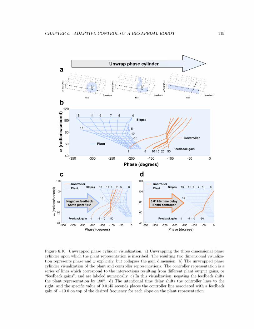
CHAPTER 6. ADAPTIVE CONTROL OF A HEXAPEDAL ROBOT 119
Imaginary Imaginary Imaginary
Crop special 2.2
Usual crop is top and bottom: 2.3375Left and right: 1.4375
Make sure that we negate plant, not contro
negated
Shifted again
-350 -300 -250 -200 -150 -100 -50 040
60
80
100
120
Phase (degrees)
ω(r
adia
ns/s
econ
d)
-15-10
05791113
15
1 5 10 15 25 50
-5
Slopes
Feedback gain
ControllerPlant
6g
pt
Unwrap phase cylinder
-350 -300 -250 -200 -150 -100 -50 040
60
80
100
120
Phase (degrees)
ω(r
adia
ns/s
econ
d) 05791113
15
-1 -5 -10 -50
-350 -300 -250 -200 -150 -100 -50 0
Slopes
Feedback gain
ControllerPlant
40
60
80
100
120ControllerPlant
-1 -5 -10 -50Feedback gain
05791113
15
Slopes
Phase (degrees)
0.0145s time delayShifts controller
Negative feedbackShifts plant 180o
a
b
c d
Figure 6.10: Unwrapped phase cylinder visualization. a) Unwrapping the three dimensional phasecylinder upon which the plant representation is inscribed. The resulting two dimensional visualiza-tion represents phase and ω explicitly, but collapses the gain dimension. b) The unwrapped phasecylinder visualization of the plant and controller representations. The controller representation is aseries of lines which correspond to the intersections resulting from different plant output gains, or“feedback gains”, and are labeled numerically. c) In this visualization, negating the feedback shiftsthe plant representation by 180◦. d) The intentional time delay shifts the controller lines to theright, and the specific value of 0.0145 seconds places the controller line associated with a feedbackgain of −10.0 on top of the desired frequency for each slope on the plant representation.
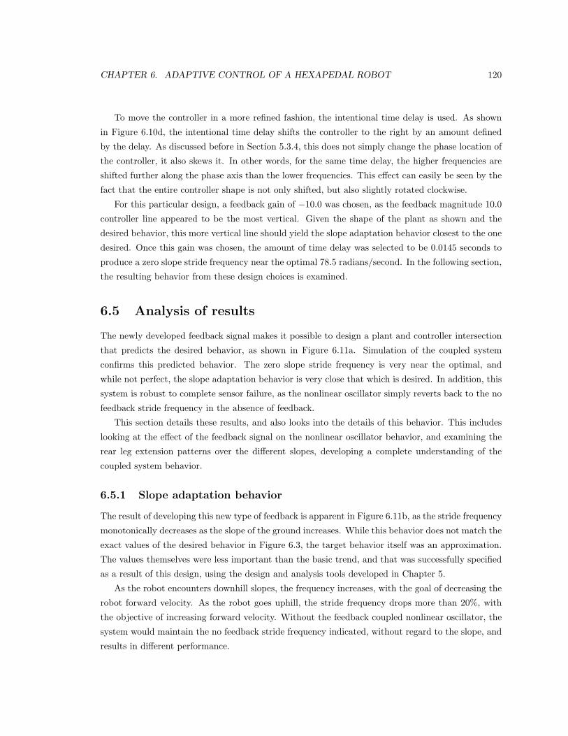
CHAPTER 6. ADAPTIVE CONTROL OF A HEXAPEDAL ROBOT 120
To move the controller in a more refined fashion, the intentional time delay is used. As shown
in Figure 6.10d, the intentional time delay shifts the controller to the right by an amount defined
by the delay. As discussed before in Section 5.3.4, this does not simply change the phase location of
the controller, it also skews it. In other words, for the same time delay, the higher frequencies are
shifted further along the phase axis than the lower frequencies. This effect can easily be seen by the
fact that the entire controller shape is not only shifted, but also slightly rotated clockwise.
For this particular design, a feedback gain of −10.0 was chosen, as the feedback magnitude 10.0
controller line appeared to be the most vertical. Given the shape of the plant as shown and the
desired behavior, this more vertical line should yield the slope adaptation behavior closest to the one
desired. Once this gain was chosen, the amount of time delay was selected to be 0.0145 seconds to
produce a zero slope stride frequency near the optimal 78.5 radians/second. In the following section,
the resulting behavior from these design choices is examined.
6.5 Analysis of results
The newly developed feedback signal makes it possible to design a plant and controller intersection
that predicts the desired behavior, as shown in Figure 6.11a. Simulation of the coupled system
confirms this predicted behavior. The zero slope stride frequency is very near the optimal, and
while not perfect, the slope adaptation behavior is very close that which is desired. In addition, this
system is robust to complete sensor failure, as the nonlinear oscillator simply reverts back to the no
feedback stride frequency in the absence of feedback.
This section details these results, and also looks into the details of this behavior. This includes
looking at the effect of the feedback signal on the nonlinear oscillator behavior, and examining the
rear leg extension patterns over the different slopes, developing a complete understanding of the
coupled system behavior.
6.5.1 Slope adaptation behavior
The result of developing this new type of feedback is apparent in Figure 6.11b, as the stride frequency
monotonically decreases as the slope of the ground increases. While this behavior does not match the
exact values of the desired behavior in Figure 6.3, the target behavior itself was an approximation.
The values themselves were less important than the basic trend, and that was successfully specified
as a result of this design, using the design and analysis tools developed in Chapter 5.
As the robot encounters downhill slopes, the frequency increases, with the goal of decreasing the
robot forward velocity. As the robot goes uphill, the stride frequency drops more than 20%, with
the objective of increasing forward velocity. Without the feedback coupled nonlinear oscillator, the
system would maintain the no feedback stride frequency indicated, without regard to the slope, and
results in different performance.
CHAPTER 6. ADAPTIVE CONTROL OF A HEXAPEDAL ROBOT 121
UphillDownhillUphillDownhill
Crop special 2.2
Usual crop is top and bottom: 2.3375Left and right: 1.4375
g-150 -100 -50 0
55
60
65
70
75
80
85
90
95
100
105 05791113
15
Feedback gain = -10.0Delay = 0.0145 seconds
Slope
DownhillUphill
-15
-10
20
ω(r
adia
ns/s
econ
d)
Phase (degrees)
-15 -10 -5 0 5 10 1550
55
60
65
70
75
80
85
90
-15 -10 -5 0 5 10 150.2
0.3
0.4
0.5
0.6
0.7
0.8
0.9
1
1.1
1.2
Slope (degrees)
ω(r
adia
ns/s
econ
d)
Velo
city
(met
ers/
seco
nd)
Slope (degrees)
No feedbackNo feedback
10% decreasein velocity
33% increasein velocity
a
b c
ControllerCoupled System
Plant
?
Figure 6.11: Pulse coupled system design and performance. a) Unwrapped phase cylinder visual-ization of the coupled system, showing the plant and controller representations for a feedback gainof −10.0 and an intentional time delay of 0.0145 seconds. The predicted solution is verified by sim-ulation of the coupled system. b) Comparison of the coupled system behavior and the no feedbackbehavior. The stride frequency of the coupled system decreases as the slope increases, the basicdesired behavioral trend (Figure 6.3). c) Comparison of the coupled system performance and the nofeedback performance. Relative to no feedback, the feedback coupling decreases the robot velocityon downhill slopes by 10% and increases the velocity on the uphill slopes by 33%, meeting the basicdesired performance goals (Section 6.1.3).
CHAPTER 6. ADAPTIVE CONTROL OF A HEXAPEDAL ROBOT 122
6.5.2 Feedback induced increases in performance
Figure 6.11c shows the change in performance, and compares this performance to the no feedback
case. Because the intersection was designed such that the zero slope frequency would be very near
the optimal, the performance of the no feedback and feedback coupled systems are equivalent at this
point.
The differences occur when the robot encounters uphill and downhill slopes. As indicated above,
on downhill slopes the robot stride frequency increases. The result of this is that the robot perfor-
mance is pulled away from the higher speed performance plateau shown in Figure 6.3 and the robot
runs slower than it would without the feedback. At a slope of −15◦, the robot forward velocity is
reduced by 10% relative to the no feedback performance on the same slope.
The change in performance on the uphill slopes is even more obvious. The stride frequency of
the robot drops significantly on these slopes, and leads to a significant increase in speed on the 15◦
inclination. Compared to the no feedback stride frequency, the feedback coupled lower frequency
results in a 33% increase in the robot’s forward velocity.
6.5.3 Detailed coupled system analysis
The result of feedback coupling the nonlinear oscillator is that the stride frequency now changes
with slope. This occurs due to the influence that the feedback has on the dynamics of the nonlinear
oscillator. In turn, this change in dynamics drives the robot at a different frequency, resulting in
the feedback signal produced. In this way, the system is truly coupled - each of the two components
affects the dynamics of the other.
Figure 6.12 shows the details of this interaction as the slope changes from downhill to flat to
uphill. One of the most apparent features of Figure 6.12a is that the stride period is quite short for
downhill slopes, longer for flat, and significantly longer for uphill slopes (each of the time axes is
equivalent).
Rear leg extension
What is less apparent becomes clear when these plots are compared to Figure 6.7, where the system
is run without feedback. In that plot, the rear legs don’t come close to extending fully - the stride
period is just too short for that to happen given the extra work the actuators have to do. With the
pulse adaptation, the stride period is extended, and the legs are given the opportunity to extend
more, which is what ultimately results in the higher uphill velocity as compared to the no feedback
case.
Additionally, as the stride period is shortened, the rear legs drag less with the feedback in place.
It is interesting that less dragging results in a lower forward velocity, and a more in-depth analysis
of other contributing factors (such as the role that the other legs play) is necessary to address this
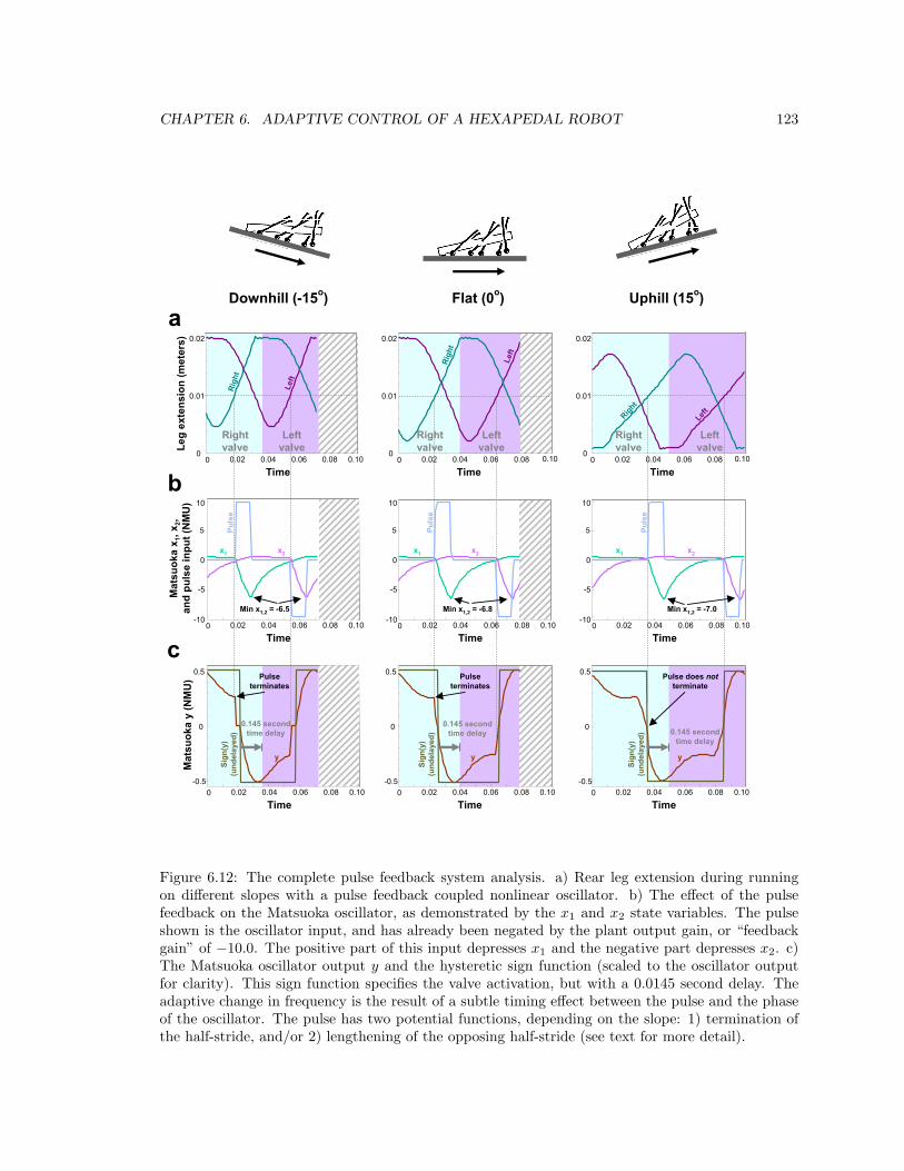
CHAPTER 6. ADAPTIVE CONTROL OF A HEXAPEDAL ROBOT 123
0 0.02 0.04 0.06 0.080
0.01
0.02
-10
-5
0
5
10
-0.5
0
0.5
Time0 0.02 0.04 0.06 0.08
Time0 0.02 0.04 0.06 0.08
Time
Leg
exte
nsio
n (m
eter
s)
0
0.01
0.02
0
0.01
0.02
0.100.100.10
Downhill (-15o) Flat (0o) Uphill (15o)
0 0.02 0.04 0.06 0.08
Time0.10 0 0.02 0.04 0.06 0.08
Time0.10 0 0.02 0.04 0.06 0.08
Time0.10
0 0.02 0.04 0.06 0.08
Time0.100 0.02 0.04 0.06 0.08
Time0.100 0.02 0.04 0.06 0.08
Time0.10
Min x1,2 = -6.5 Min x1,2 = -6.8 Min x1,2 = -7.0
Mat
suok
a x 1
, x2,
and
puls
e in
put (
NM
U)
-10
-5
0
5
10
-10
-5
0
5
10
Left
Righ
t
Left
Righ
t
LeftRigh
t
x1 x2
Puls
e
Puls
e
Puls
e
x1 x2 x1 x2
Sign
(y)
(und
elay
ed)
Sign
(y)
(und
elay
ed)
Sign
(y)
(und
elay
ed)
y y y
Mat
suok
a y
(NM
U) Pulse
terminatesPulse
terminatesPulse does not
terminate
-0.5
0
0.5
-0.5
0
0.5
Leftvalve
Rightvalve
Leftvalve
Rightvalve
Leftvalve
0.145 secondtime delay
0.145 secondtime delay
0.145 secondtime delay
a
b
c
Rightvalve
Figure 6.12: The complete pulse feedback system analysis. a) Rear leg extension during runningon different slopes with a pulse feedback coupled nonlinear oscillator. b) The effect of the pulsefeedback on the Matsuoka oscillator, as demonstrated by the x1 and x2 state variables. The pulseshown is the oscillator input, and has already been negated by the plant output gain, or “feedbackgain” of −10.0. The positive part of this input depresses x1 and the negative part depresses x2. c)The Matsuoka oscillator output y and the hysteretic sign function (scaled to the oscillator outputfor clarity). This sign function specifies the valve activation, but with a 0.0145 second delay. Theadaptive change in frequency is the result of a subtle timing effect between the pulse and the phaseof the oscillator. The pulse has two potential functions, depending on the slope: 1) termination ofthe half-stride, and/or 2) lengthening of the opposing half-stride (see text for more detail).
CHAPTER 6. ADAPTIVE CONTROL OF A HEXAPEDAL ROBOT 124
anomaly.
Feedback influence on the nonlinear oscillator
The relationship between the leg extensions and the pulse feedback is a threshold crossing based pulse
of the appropriate sign, as shown in Figure 6.12a,b. When the left leg crosses the extension threshold,
a positive pulse of amplitude 1.0 and fixed time length (0.01 seconds) is generated. Conversely, when
the right leg crosses this threshold, a negative pulse is generated. The pulse signal shown in Figure
6.12b is the input to the controller, and has been negated and scaled by the plant output, or
“feedback” gain.
As shown in Equations 6.1-6.9 and Figure 6.12b, this input directly affects the oscillator state
variables x1 and x2. In turn, the difference in these state variables is the Matsuoka oscillator output,
y, which in turn drives the robot valves through a sign function with hysteresis (see Section 6.2.1).
The positive part of the feedback is negatively applied to x1, and the negative part of the
feedback is negatively applied to x2. In other words, of the two pulses that occur during each stride,
the positive pulse depresses x1 and the negative pulse depresses x2. This effect is apparent in Figure
6.12b, which plots the x1 and x2 state variables and the pulse feedback.
In the zero slope running case, the pulse performs two functions: 1) termination of the half-stride,
and 2) lengthening of the opposing half-stride. For example, the positive pulse terminates the half
stride by depressing x1 below zero, which also removes the mutual inhibition (associated with the
γ term) and allows x2 to rise above zero more rapidly. In addition, the pulse also lengthens the
half stride associated with x2 being above zero by depressing x1 to −6.8, as the magnitude of this
depression (partially) determines how long it takes for x1 to rise above zero again. As the halves of
the strides and of the nonlinear oscillator are symmetric, x2 has the same effect on x1 as x1 has on
x2, both here and below.
The adaptive change in frequency in response to varying slope is the result of a subtle timing
effect. This effect comes from the phase difference in the feedback signal as different slopes are
encountered, as described in Section 6.3.2 and Figure 6.7. In the uphill case shown in Figure 6.12,
the positive pulse occurs much later, when the difference between x1 and x2 has already dictated a
sign change. Thus, the action of the feedback in this case is purely to lengthen the x2 half stride
by depressing x1 further than the zero slope case of −6.8 to −7.0. More time is required for x1 to
rise above zero again from this lower value, and therefore the x2 half-stride is lengthened for uphill
slopes.
In the downhill case, the pulse occurs sooner, causing the half stride to be terminated earlier3.
In addition, because the pulse begins to depress x1 while it is still above zero, at the end of the pulse3It should be noted that the hysteretic sign function counteracts the termination effect to some extent (the sign does
not change until the zero threshold has actually been crossed). It is left to future work to determine the implicationsof using different rules to determine how to actuate the valves when y=0.
CHAPTER 6. ADAPTIVE CONTROL OF A HEXAPEDAL ROBOT 125
the total x1 depression is only −6.5. As a result, less time is required for x1 to again rise above zero
and this shortens the half-stride associated with x2.
Intentional time delay
Completing the coupled system loop, the output of the controller is shown in Figure 6.12c. The
Matsuoka oscillator output y is plotted along with the hysteretic sign of nonlinear oscillator output.
The output of this sign function is mathematically treated as amplitude 1, but in the figure it is
normalized to the amplitude of the oscillator output for clarity.
This binary output is in turn used to drive the valves, activating them after the intentional time
delay of 0.145 seconds is applied, as shown in Figure 6.12c. As this is the signal that causes the legs
in Figure 6.12a to extend, the complete cycle is shown.
It is interesting to note that there are (at least) two delays at work here. The most obvious,
of course, is the intentional time delay. The less obvious one, however, is the delay induced by the
pneumatics and the inertial of the piston-foot assembly of the robot. As this assembly has dynamics
of its own, there is a significant delay between when the valves are opened and when the legs begin
to extend. Also, when the valves close, the piston-foot assembly inertia causes the legs to continue
to extend. Rather than being a large control design concern, this and other delays are implicitly
compensated for in the coupled design process illustrated here. Interestingly, significant activation
delays present in animal muscle are also compensated for by control signals that come well before
the expected action is produced (Full et al., 1998b).
6.5.4 Sensor failure performance
One of the main benefits of using a feedback coupled nonlinear oscillator is the performance in
response to complete sensor failure. As noted in Section 4.1, this is a common property of animal
nervous systems, and is a highly desirable trait in the real world, where sensors are fragile and the
environment unforgiving.
Complete sensor failure simply eliminates the feedback to the system, and the controller auto-
matically reverts to the no feedback stride frequency. While the robot will not respond to changing
slopes as desired, this is preferable to ceasing operation altogether, which would be the case for most
other types of feedback driven controllers.
The effect of a partial sensor failure is unknown at this point. Presumably, with a high-pass
filter in place failure of one leg sensor would continue to yield an oscillatory input to the controller.
However, this phase would likely be quite incorrect to generate the adaptation trends desired, and
would likely be worse than the no feedback configuration. However, as with complete sensor failure,
a (suboptimal) valve signal would continue to be generated and forward locomotion would continue.
This may be analogous to the observations of Delcomyn (Delcomyn, 1971) (Delcomyn, 1985) (Del-
comyn, 1999), who notes that animals with prosthetic legs (and therefore partial sensory feedback)
CHAPTER 6. ADAPTIVE CONTROL OF A HEXAPEDAL ROBOT 126
still maintain the ability to locomote, but they appear to be much less coordinated. In any case, an-
alyzing the behavior of the simulated robot system in the case of partial sensor failure will certainly
be interesting, and is left as an exercise for future work.
The design tools developed in the previous chapter were successfully used to create a feedback
coupled system that has desired adaptive behavior. While the example here was a running robot
and the animal experiments were with running cockroaches, designing adaptive controllers is not
limited to locomotion. The design process would have been the same for any other cyclic dynamic
system and any other desired behavior, and the generality of the controller, method, and design
tools is discussed in the conclusions of this thesis.
Chapter 7
Conclusions
It is a reminder to me that all things end.
-Spock (Star Trek VI: The Undiscovered Country)
This thesis provides a biologically-inspired approach for achieving adaptive behaviors for cyclic
dynamic tasks: biomimetic control with a feedback coupled nonlinear oscillator. While this work was
focused on running animals and the robots they have inspired, the design method and analysis tools
developed are not specific to these systems. Instead, they represent a general scheme for designing
adaptive controllers for cyclic dynamic tasks.
7.1 Conclusions
Animal nervous systems are extraordinarily complex, and in truth, very little is understood about
how they function. The work done here represents only one small step, in this case toward un-
derstanding the role of sensory feedback during cyclic behaviors. The animal experiments showed
that the cockroach, Blaberus discoidalis, does use sensory feedback even at the highest speeds of
locomotion, even though neural delays are large relative to the stride period at these speeds. In
addition, the behavior observed is consistent with the behavior that is expected from a feedback
coupled nonlinear oscillator model of the circuits that generate the motor patterns.
A functional role that has been hypothesized for this type of behavior is adaptation, and was
explored by designing a controller for a simulation of a biomimetic robot running on varying slopes.
The same nonlinear oscillator used to predict the animal experiment results was used as the controller
for the robot, and the feedback coupled system exhibited the desired adaptive behavior. As the robot
encountered different slopes, the interaction between the dynamics of locomotion and the dynamics
of the nonlinear oscillator resulted in running at different frequencies. This successful use of the
127
CHAPTER 7. CONCLUSIONS 128
feedback coupled nonlinear oscillator indicates that the sensor-based oscillatory behaviors observed
in animals may have adaptive functions.
To create this coupled system behavior, an existing visual design method (Williamson, 1999)
was extended to address design for adaptation. The extension of this method explicitly takes the
dynamics of the plant and controller into account, creating three dimensional visual representations
of each system as conditions change. The ω contour analysis tool shows how these two set of dynamics
interact when they are coupled together, and indicates the feedback properties necessary to result
in the desired behavior. In addition, an intentional time delay alters this dynamic interaction, and
can be used to fine-tune the coupled system behavior.
In addition to being an adaptive controller, the feedback coupled nonlinear oscillator is also robust
to sensor failure. An important consideration for real robots, if the sensor fails or if the connection
is broken, then the controller reverts to self-sustained oscillations. The adaptive behavior no longer
occurs, but the robot does not cease functioning.
This approach and these tools represent much more than a way to get the robot to run well -
they represent a general approach for cyclic task control. While other approaches have been devised
to give the specific robot the same behavior, those techniques do not generalize to other systems. In
contrast, none of the techniques and tools used here are specific to this example problem, and are
applicable to cyclic dynamic tasks in general.
In addition, the feedback coupled nonlinear oscillator incorporates a number of “features” in one
design solution. The slope adaptation behavior could be replaced by a lookup table; the selective
frequency entrainment could be replaced by an appropriate filter; and the robustness to sensor failure
could be replaced by a clever heuristic. However, each of these is already contained in the feedback
coupled nonlinear oscillator, eliminating the need for an a la carte approach to the controller design.
The biological basis for this control structure provides some insight that this may be a more
general and elegant solution than other approaches. This thesis is only one intermediate step,
though, and more work is needed to fully understand the relative merits of this approach.
7.2 Future work
The implications of using sensory-mediated motor commands for legged locomotion are one of the
many exciting areas indicated for future work. In particular, the experimental setup used for the
animal experiments in this thesis is well-suited for performing more sophisticated experiments, as it
is coupled to a real-time operating system. It is possible to take advantage of this “computer in the
loop,” designing experiments that require real-time interaction to probe specific predictions about
the sensory-based neural mechanisms.
These experiments are not limited to simply generating sustained perturbations, but can actually
CHAPTER 7. CONCLUSIONS 129
instantaneously generate perturbations based on the EMG signals recorded. Very interesting exper-
iments can be devised, including using the force-displacement actuator to add artificial muscles with
computer-selected amounts of delay. The challenge here, of course, is to design the appropriate ex-
periment, determining how to test a specific hypothesis and relating this hypothesis to implications
on the resulting performance of the animal.
Simulated experiments such as the ones conducted for this thesis are powerful tools for verifying
expected results of complicated animal experiments, as they can be used to eliminate analysis tech-
niques that give confusing results. The simulated experiments here proved to be more interesting
than was expected and in themselves are a possible area of future research. For example, it was
expected that limiting the phases included in the analysis based on proximity to the perturbation
frequency would enhance the results, increasing the resolution of the test by taking advantage of
the selective entrainment properties of the nonlinear oscillator. In fact, this method made even the
simulated data much harder to interpret, as the hypothesis of uniformity was commonly rejected
for the no perturbation control cases, a surprising result that is an area of interest from a purely
mathematical standpoint.
Another possible area of exploration is to create a resonance tongue, described in Section 3.2.2, to
further analyze how receptive the animal is to oscillatory stimuli of different amplitudes. Intuitively,
the amplitude-based selective entrainment properties of nonlinear oscillators predict that as the
stimulus changes strength, the entrainment region should grow accordingly. It is unclear what
processing technique would be useful for identifying this trend, but simulations similar to the one
presented here may be useful for making that determination.
Besides new experiments, there are several other measurements that can be made from the data
that have already been collected. These data include characteristics of the EMG signal, such as
interburst interval, firing rate, number of spikes per stride, and much of the force and displacement
information.
Finally, sensory ablation experiments may help reveal the contributions of the various types of
sensors present in the cockroach. These sensors include tactile, displacement, and force mechanore-
ceptors. In comparison, robot sensorization has been severely limited by practical considerations, as
robustly integrating sensors into mechanical structures has always been a difficult problem in robot
design. Recent advances in manufacturing techniques toward creating heavily sensorized structures
are beginning to overcome this limitation (Bailey et al., 2000), further motivating these experiments
toward selecting appropriate sensorization.
Along these lines, the feedback coupled nonlinear oscillators are not limited to receiving one type
of feedback. While position information has been focused on in this study, any other type of cyclic
feedback can be used. What may be most interesting to explore is the combination of different
types of feedback, perhaps incorporating diverse signals such as contact and position information.
Other potential feedback measures include those that cycle at harmonics of the stride frequency,
CHAPTER 7. CONCLUSIONS 130
such as fore-aft accelerations, which were not considered here. However, some nonlinear oscillators
are capable of entraining to harmonics, and these potential signals should be considered.
Simulation results indicate that not only does the speed on uphill slopes increase, but the maxi-
mum climbable slope is increased by the action of the adaptive controller. The adaptive controller
may not just increase the performance in terms of velocity, but may also increase the range of terrains
that can be traversed.
In this study, slope is the only parameter that is varied, but there is no reason that other
parameters and combinations of parameters, such as mass and geometric configuration, cannot be
explored. How to visually represent the plant with multiple changes in dynamic parameters is an
interesting area in itself for future work.
Finally, studies with different types of robots may reveal whether the most effective types of
feedback are common across legged robots, or if there are specific considerations for each implemen-
tation. Additionally, these techniques can be applied to other cyclic dynamic robotic tasks, as they
are general and not limited to legged robotics.
These engineering studies may in turn suggest other experiments in biology, ones that may
not specifically involve legged locomotion. These experiments may enhance the understanding of
the seemingly universal principles of sensory-based cyclic motor control, for both engineering and
biology.
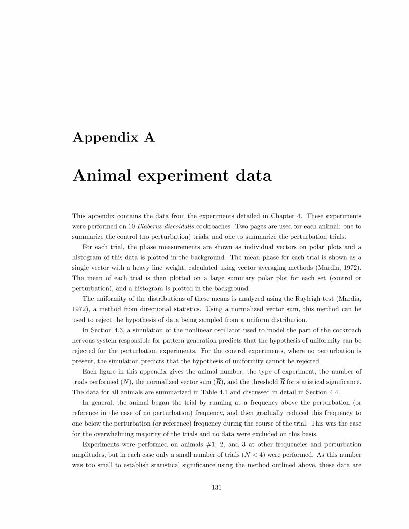
Appendix A
Animal experiment data
This appendix contains the data from the experiments detailed in Chapter 4. These experiments
were performed on 10 Blaberus discoidalis cockroaches. Two pages are used for each animal: one to
summarize the control (no perturbation) trials, and one to summarize the perturbation trials.
For each trial, the phase measurements are shown as individual vectors on polar plots and a
histogram of this data is plotted in the background. The mean phase for each trial is shown as a
single vector with a heavy line weight, calculated using vector averaging methods (Mardia, 1972).
The mean of each trial is then plotted on a large summary polar plot for each set (control or
perturbation), and a histogram is plotted in the background.
The uniformity of the distributions of these means is analyzed using the Rayleigh test (Mardia,
1972), a method from directional statistics. Using a normalized vector sum, this method can be
used to reject the hypothesis of data being sampled from a uniform distribution.
In Section 4.3, a simulation of the nonlinear oscillator used to model the part of the cockroach
nervous system responsible for pattern generation predicts that the hypothesis of uniformity can be
rejected for the perturbation experiments. For the control experiments, where no perturbation is
present, the simulation predicts that the hypothesis of uniformity cannot be rejected.
Each figure in this appendix gives the animal number, the type of experiment, the number of
trials performed (N), the normalized vector sum (R), and the threshold R for statistical significance.
The data for all animals are summarized in Table 4.1 and discussed in detail in Section 4.4.
In general, the animal began the trial by running at a frequency above the perturbation (or
reference in the case of no perturbation) frequency, and then gradually reduced this frequency to
one below the perturbation (or reference) frequency during the course of the trial. This was the case
for the overwhelming majority of the trials and no data were excluded on this basis.
Experiments were performed on animals #1, 2, and 3 at other frequencies and perturbation
amplitudes, but in each case only a small number of trials (N < 4) were performed. As this number
was too small to establish statistical significance using the method outlined above, these data are
131
APPENDIX A. ANIMAL EXPERIMENT DATA 132
not shown.
Additionally, video was captured using a high speed camera for 1-2 trials per animal. Because
bright lamps were necessary to capture the video, these trials were not included in the analyses.
It should also be noted that animals #7 and #8 had intermittent EMG signals. The characteristic
structure of EMG signal was present, but a set of pulses was not recorded for each stride the animal
made. As a result, the total number of phase measurements for each trial was generally slightly
less than those for other animals, which can be seen in Figures A.13, A.14, A.15, and A.16. The
analysis of the results, however, was not affected by this intermittent signal and these animals were
not excluded.
The only cases for exclusion included 1) animals that would not run after the EMG electrode
implantation, and 2) failed electrode implantation procedures after which no useful EMG signal
could be recorded. In these cases, the experiment was terminated and no data was collected from
that animal.
For the animals and experiments that are shown here, none of the relevant data or trials were
excluded for any reason.

APPENDIX A. ANIMAL EXPERIMENT DATA 133
6
90
270
180 0
7
90
270
180 0
7
90
270
180 0
5
90
270
180 0
6
90
270
180 0
10
90
270
180 0
11
90
270
180 0
7
90
270
180 0
6
90
270
180 0
5
90
270
180 0
7
90
270
180 0
7
90
270
180 0
1
2
30
210
60
240
90
270
120
300
150
330
180 0
Animal #_22_15Hz_no_pert
AllN = 12R/N = 0.19
Animal #1No perturbation
Expected result: Uniform
Uniform
Rayleigh testN = 12R = 0.19p > 0.05 R(p=0.05, N=12)=0.494
Figure A.1: Animal #1 no perturbation control data.
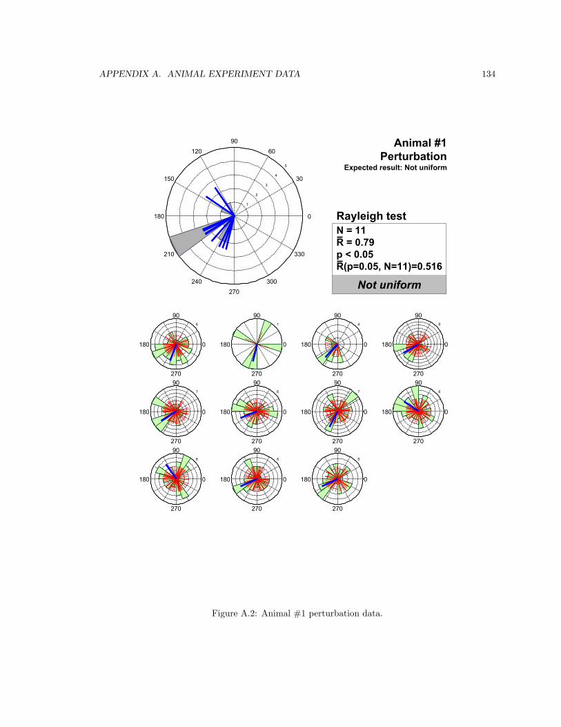
APPENDIX A. ANIMAL EXPERIMENT DATA 134
6
90
270
180 0
1
90
270
180 0
4
90
270
180 0
8
90
270
180 0
7
90
270
180 0
6
90
270
180 0
7
90
270
180 0
6
90
270
180 0
6
90
270
180 0
6
90
270
180 0
5
90
270
180 0
1
2
3
4
5
30
210
60
240
90
270
120
300
150
330
180 0
Animal #exp_22_15Hz_pert
AllN = 11R/N = 0.79
Animal #1Perturbation
Expected result: Not uniform
Not uniform
Rayleigh testN = 11R = 0.79p < 0.05 R(p=0.05, N=11)=0.516
Figure A.2: Animal #1 perturbation data.
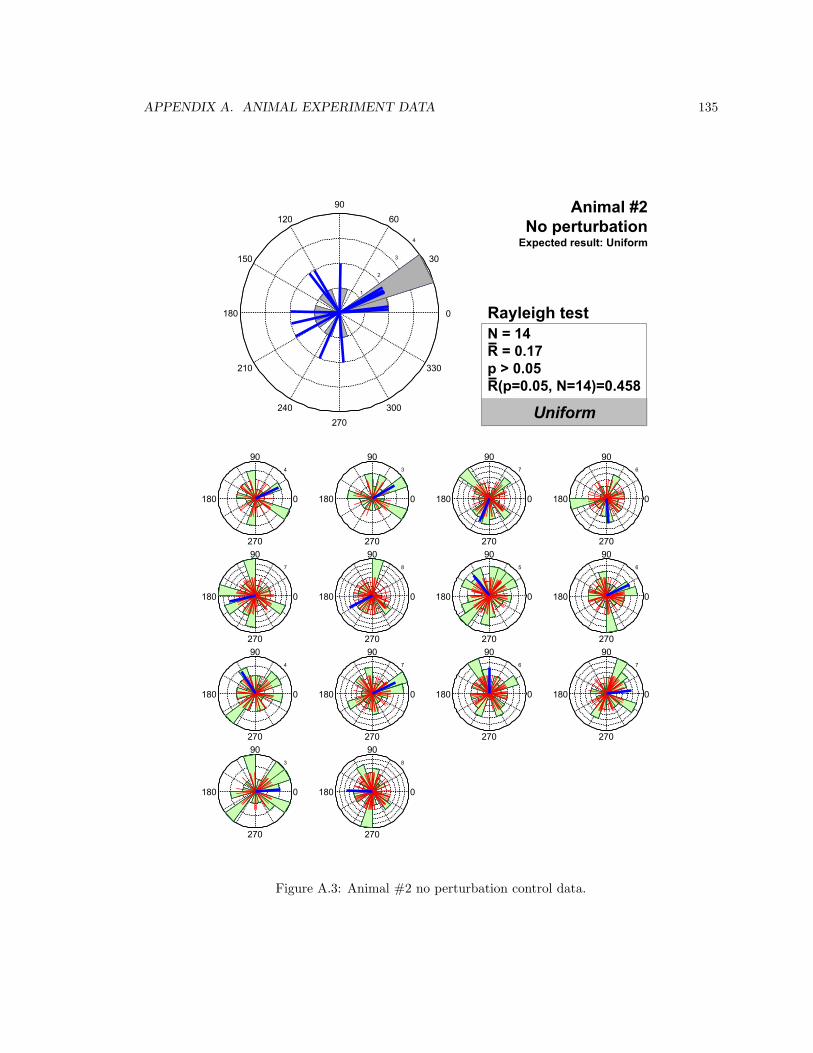
APPENDIX A. ANIMAL EXPERIMENT DATA 135
4
90
270
180 0
3
90
270
180 0
7
90
270
180 0
6
90
270
180 0
7
90
270
180 0
8
90
270
180 0
5
90
270
180 0
6
90
270
180 0
4
90
270
180 0
7
90
270
180 0
6
90
270
180 0
7
90
270
180 0
3
90
270
180 0
8
90
270
180 0
1
2
3
4
30
210
60
240
90
270
120
300
150
330
180 0
Animal #_24_15Hz_no_pert
AllN = 14R/N = 0.17
Animal #2No perturbation
Expected result: Uniform
Uniform
Rayleigh testN = 14R = 0.17p > 0.05 R(p=0.05, N=14)=0.458
Figure A.3: Animal #2 no perturbation control data.
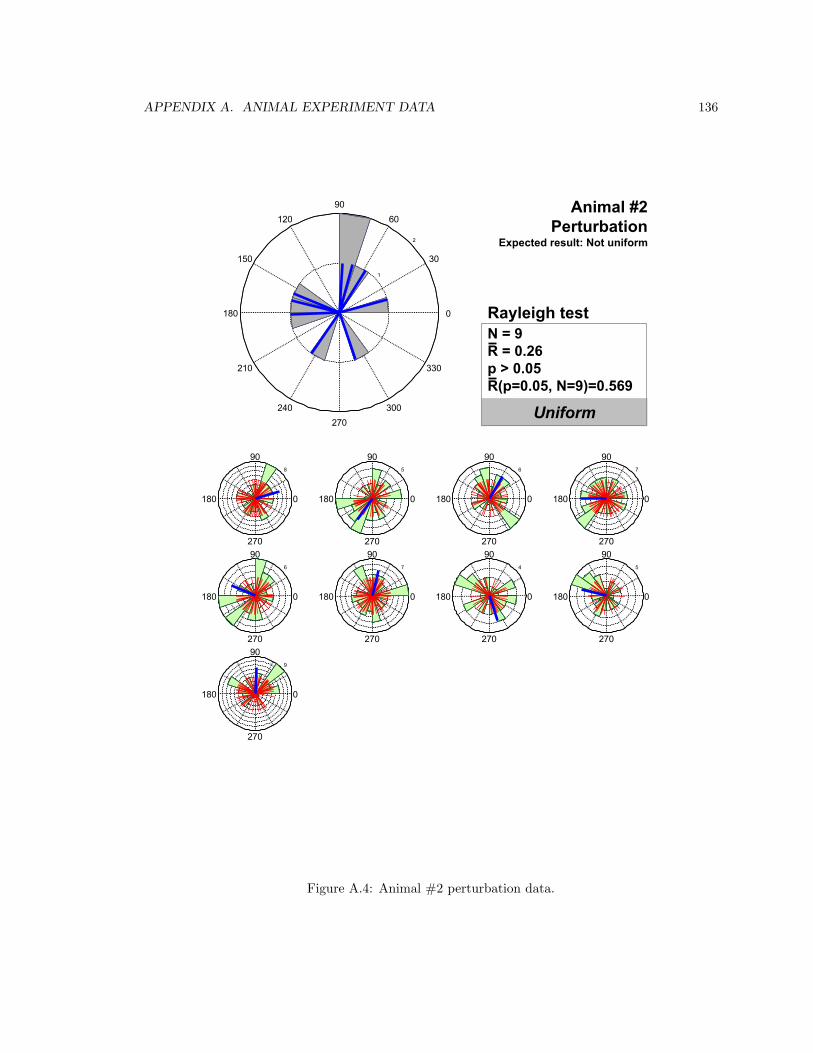
APPENDIX A. ANIMAL EXPERIMENT DATA 136
8
90
270
180 0
5
90
270
180 0
6
90
270
180 0
7
90
270
180 0
6
90
270
180 0
7
90
270
180 0
4
90
270
180 0
5
90
270
180 0
9
90
270
180 0
1
2
30
210
60
240
90
270
120
300
150
330
180 0
Animal #exp_24_15Hz_pert
AllN = 9R/N = 0.26
Animal #2Perturbation
Expected result: Not uniform
Uniform
Rayleigh testN = 9R = 0.26p > 0.05 R(p=0.05, N=9)=0.569
Figure A.4: Animal #2 perturbation data.
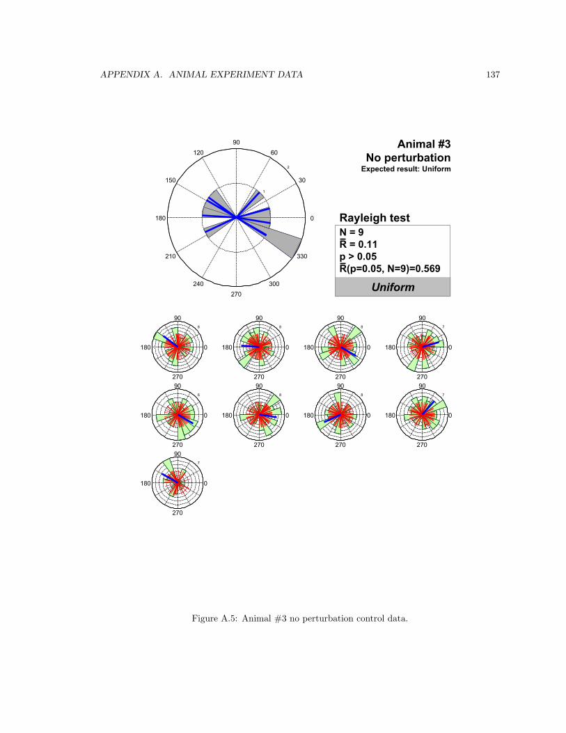
APPENDIX A. ANIMAL EXPERIMENT DATA 137
8
90
270
180 0
8
90
270
180 0
8
90
270
180 0
7
90
270
180 0
6
90
270
180 0
8
90
270
180 0
8
90
270
180 0
7
90
270
180 0
7
90
270
180 0
1
2
30
210
60
240
90
270
120
300
150
330
180 0
Animal #_27_15Hz_no_pert
AllN = 9R/N = 0.11
Animal #3No perturbation
Expected result: Uniform
Uniform
Rayleigh testN = 9R = 0.11p > 0.05 R(p=0.05, N=9)=0.569
Figure A.5: Animal #3 no perturbation control data.
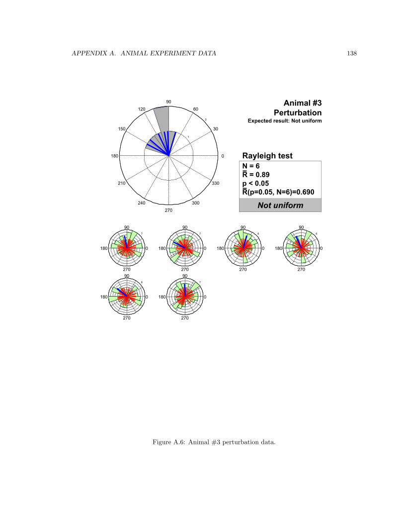
APPENDIX A. ANIMAL EXPERIMENT DATA 138
7
90
270
180 0
7
90
270
180 0
6
90
270
180 0
6
90
270
180 0
8
90
270
180 0
7
90
270
180 0
1
2
30
210
60
240
90
270
120
300
150
330
180 0
Animal #exp_27_15Hz_pert
AllN = 6R/N = 0.89
Animal #3Perturbation
Expected result: Not uniform
Not uniform
Rayleigh testN = 6R = 0.89p < 0.05 R(p=0.05, N=6)=0.690
Figure A.6: Animal #3 perturbation data.
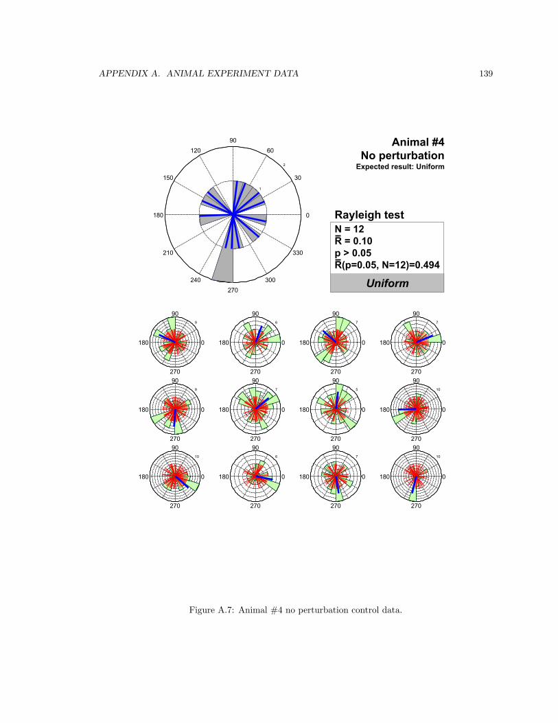
APPENDIX A. ANIMAL EXPERIMENT DATA 139
9
90
270
180 0
6
90
270
180 0
7
90
270
180 0
7
90
270
180 0
9
90
270
180 0
7
90
270
180 0
5
90
270
180 0
10
90
270
180 0
10
90
270
180 0
6
90
270
180 0
7
90
270
180 0
10
90
270
180 0
1
2
30
210
60
240
90
270
120
300
150
330
180 0
Animal #_29_19hz_no_pert
AllN = 12R/N = 0.10
Animal #4No perturbation
Expected result: Uniform
Uniform
Rayleigh testN = 12R = 0.10p > 0.05 R(p=0.05, N=12)=0.494
Figure A.7: Animal #4 no perturbation control data.
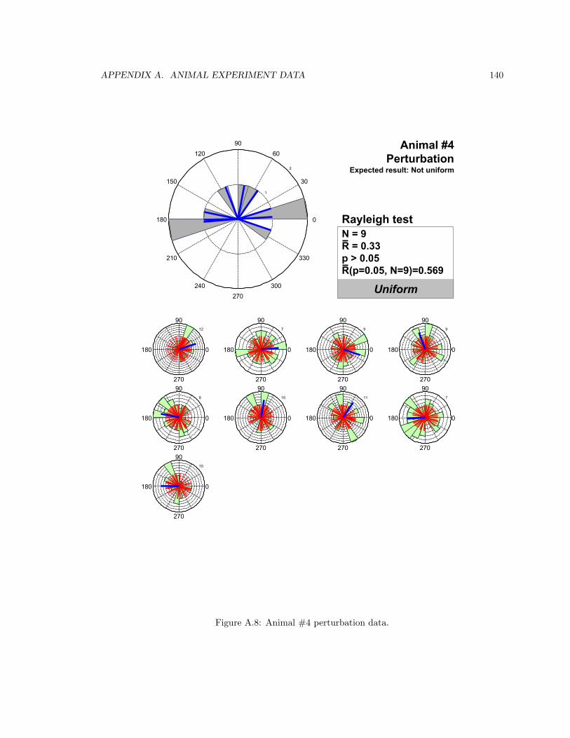
APPENDIX A. ANIMAL EXPERIMENT DATA 140
12
90
270
180 0
7
90
270
180 0
9
90
270
180 0
9
90
270
180 0
8
90
270
180 0
10
90
270
180 0
11
90
270
180 0
7
90
270
180 0
10
90
270
180 0
1
2
30
210
60
240
90
270
120
300
150
330
180 0
Animal #exp_29_19hz_pert
AllN = 9R/N = 0.33
Animal #4Perturbation
Expected result: Not uniform
Uniform
Rayleigh testN = 9R = 0.33p > 0.05 R(p=0.05, N=9)=0.569
Figure A.8: Animal #4 perturbation data.
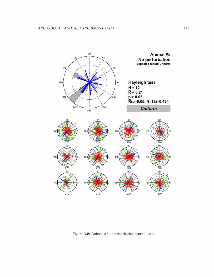
APPENDIX A. ANIMAL EXPERIMENT DATA 141
9
90
270
180 0
9
90
270
180 0
12
90
270
180 0
6
90
270
180 0
7
90
270
180 0
8
90
270
180 0
9
90
270
180 0
6
90
270
180 0
3
90
270
180 0
8
90
270
180 0
9
90
270
180 0
6
90
270
180 0
1
2
3
30
210
60
240
90
270
120
300
150
330
180 0
Animal #_30_19Hz_no_pert
AllN = 12R/N = 0.21
Animal #5No perturbation
Expected result: Uniform
Uniform
Rayleigh testN = 12R = 0.21p > 0.05 R(p=0.05, N=12)=0.494
Figure A.9: Animal #5 no perturbation control data.
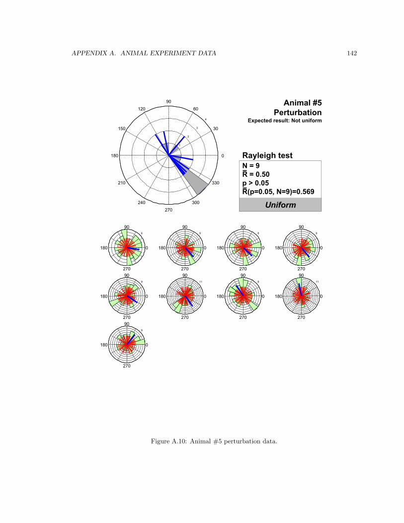
APPENDIX A. ANIMAL EXPERIMENT DATA 142
6
90
270
180 0
9
90
270
180 0
8
90
270
180 0
9
90
270
180 0
9
90
270
180 0
11
90
270
180 0
8
90
270
180 0
11
90
270
180 0
9
90
270
180 0
1
2
3
4
30
210
60
240
90
270
120
300
150
330
180 0
Animal #exp_30_19hz_pert
AllN = 9R/N = 0.50
Animal #5Perturbation
Expected result: Not uniform
Uniform
Rayleigh testN = 9R = 0.50p > 0.05 R(p=0.05, N=9)=0.569
Figure A.10: Animal #5 perturbation data.
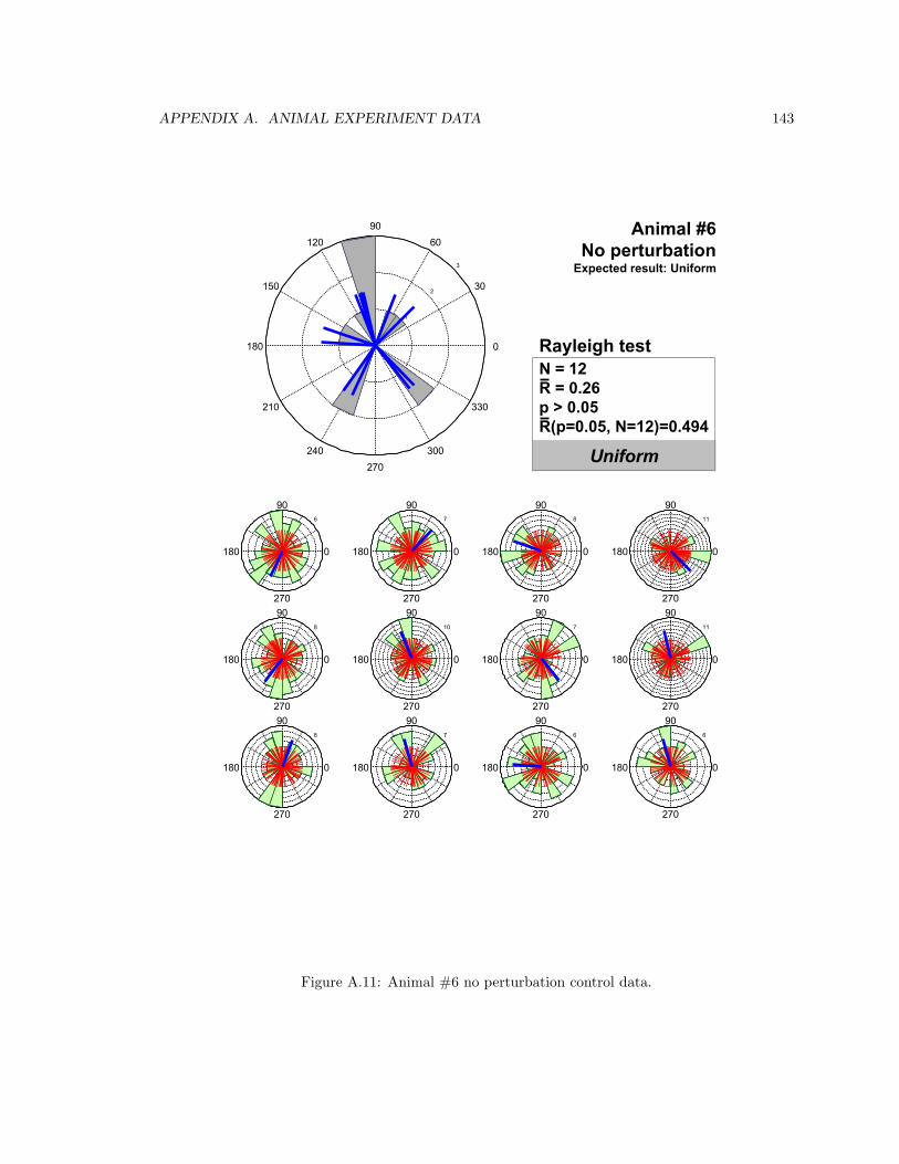
APPENDIX A. ANIMAL EXPERIMENT DATA 143
6
90
270
180 0
7
90
270
180 0
8
90
270
180 0
11
90
270
180 0
8
90
270
180 0
10
90
270
180 0
7
90
270
180 0
11
90
270
180 0
8
90
270
180 0
7
90
270
180 0
6
90
270
180 0
6
90
270
180 0
1
2
3
30
210
60
240
90
270
120
300
150
330
180 0
Animal #_31_15Hz_no_pert
AllN = 12R/N = 0.26
Animal #6No perturbation
Expected result: Uniform
Uniform
Rayleigh testN = 12R = 0.26p > 0.05 R(p=0.05, N=12)=0.494
Figure A.11: Animal #6 no perturbation control data.
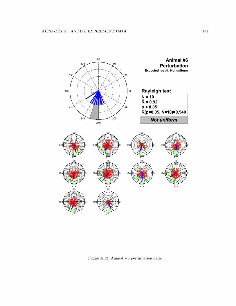
APPENDIX A. ANIMAL EXPERIMENT DATA 144
11
90
270
180 0
12
90
270
180 0
7
90
270
180 0
12
90
270
180 0
13
90
270
180 0
11
90
270
180 0
9
90
270
180 0
10
90
270
180 0
13
90
270
180 0
7
90
270
180 0
1
2
3
4
30
210
60
240
90
270
120
300
150
330
180 0
Animal #exp_31_15Hz_pert
AllN = 10R/N = 0.92
Animal #6Perturbation
Expected result: Not uniform
Not uniform
Rayleigh testN = 10R = 0.92p < 0.05 R(p=0.05, N=10)=0.540
Figure A.12: Animal #6 perturbation data.
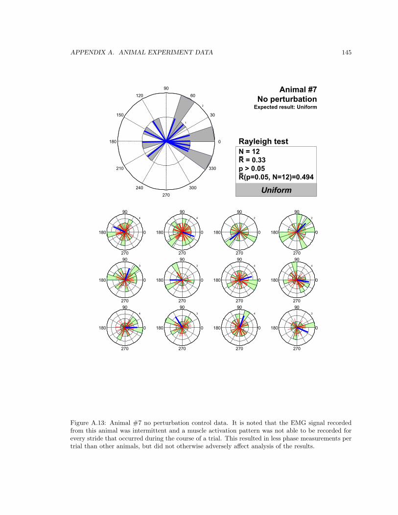
APPENDIX A. ANIMAL EXPERIMENT DATA 145
4
90
270
180 0
4
90
270
180 0
2
90
270
180 0
2
90
270
180 0
3
90
270
180 0
3
90
270
180 0
4
90
270
180 0
4
90
270
180 0
4
90
270
180 0
3
90
270
180 0
4
90
270
180 0
3
90
270
180 0
1
2
30
210
60
240
90
270
120
300
150
330
180 0
Animal #_32_17Hz_no_pert
AllN = 12R/N = 0.33
Animal #7No perturbation
Expected result: Uniform
Uniform
Rayleigh testN = 12R = 0.33p > 0.05 R(p=0.05, N=12)=0.494
Figure A.13: Animal #7 no perturbation control data. It is noted that the EMG signal recordedfrom this animal was intermittent and a muscle activation pattern was not able to be recorded forevery stride that occurred during the course of a trial. This resulted in less phase measurements pertrial than other animals, but did not otherwise adversely affect analysis of the results.
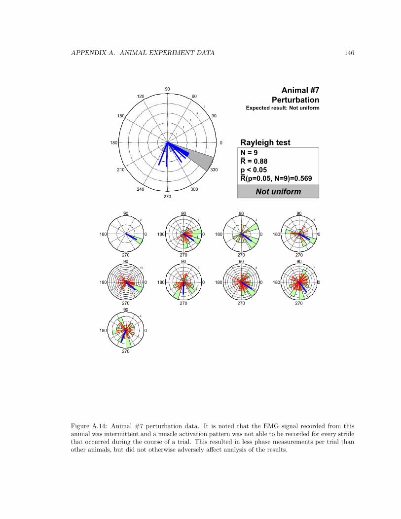
APPENDIX A. ANIMAL EXPERIMENT DATA 146
2
90
270
180 0
5
90
270
180 0
2
90
270
180 0
4
90
270
180 0
10
90
270
180 0
5
90
270
180 0
8
90
270
180 0
7
90
270
180 0
4
90
270
180 0
1
2
3
4
5
30
210
60
240
90
270
120
300
150
330
180 0
Animal #exp_32_17Hz_pert
AllN = 9R/N = 0.88
Animal #7Perturbation
Expected result: Not uniform
Not uniform
Rayleigh testN = 9R = 0.88p < 0.05 R(p=0.05, N=9)=0.569
Figure A.14: Animal #7 perturbation data. It is noted that the EMG signal recorded from thisanimal was intermittent and a muscle activation pattern was not able to be recorded for every stridethat occurred during the course of a trial. This resulted in less phase measurements per trial thanother animals, but did not otherwise adversely affect analysis of the results.
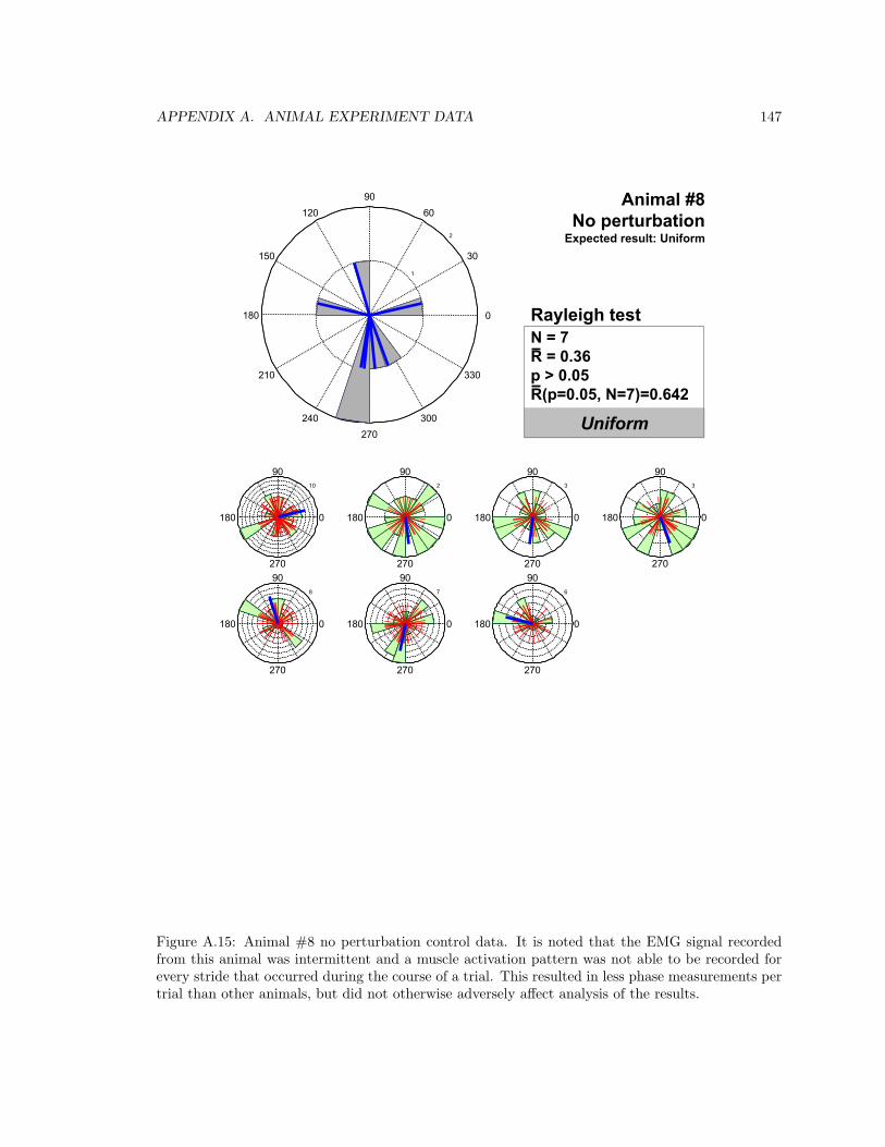
APPENDIX A. ANIMAL EXPERIMENT DATA 147
10
90
270
180 0
2
90
270
180 0
3
90
270
180 0
3
90
270
180 0
8
90
270
180 0
7
90
270
180 0
6
90
270
180 0
1
2
30
210
60
240
90
270
120
300
150
330
180 0
Animal #_33_17Hz_no_pert
AllN = 7R/N = 0.36
Animal #8No perturbation
Expected result: Uniform
Uniform
Rayleigh testN = 7R = 0.36p > 0.05 R(p=0.05, N=7)=0.642
Figure A.15: Animal #8 no perturbation control data. It is noted that the EMG signal recordedfrom this animal was intermittent and a muscle activation pattern was not able to be recorded forevery stride that occurred during the course of a trial. This resulted in less phase measurements pertrial than other animals, but did not otherwise adversely affect analysis of the results.
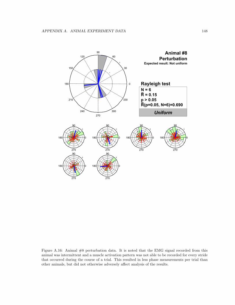
APPENDIX A. ANIMAL EXPERIMENT DATA 148
5
90
270
180 0
5
90
270
180 0
6
90
270
180 0
5
90
270
180 0
6
90
270
180 0
6
90
270
180 0
1
2
30
210
60
240
90
270
120
300
150
330
180 0
Animal #exp_33_17Hz_pert
AllN = 6R/N = 0.15
Animal #8Perturbation
Expected result: Not uniform
Uniform
Rayleigh testN = 6R = 0.15p > 0.05 R(p=0.05, N=6)=0.690
Figure A.16: Animal #8 perturbation data. It is noted that the EMG signal recorded from thisanimal was intermittent and a muscle activation pattern was not able to be recorded for every stridethat occurred during the course of a trial. This resulted in less phase measurements per trial thanother animals, but did not otherwise adversely affect analysis of the results.
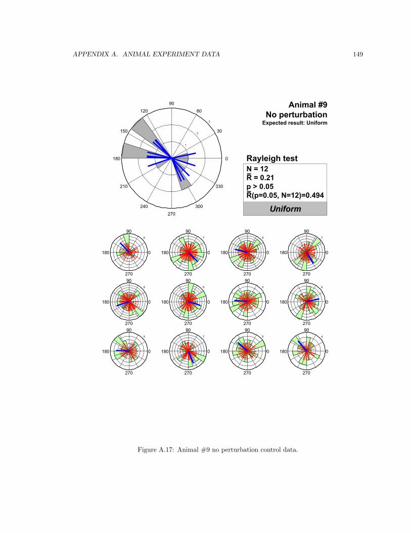
APPENDIX A. ANIMAL EXPERIMENT DATA 149
6
90
270
180 0
7
90
270
180 0
8
90
270
180 0
7
90
270
180 0
8
90
270
180 0
8
90
270
180 0
5
90
270
180 0
6
90
270
180 0
5
90
270
180 0
7
90
270
180 0
5
90
270
180 0
4
90
270
180 0
1
2
3
30
210
60
240
90
270
120
300
150
330
180 0
Animal #_34_17Hz_no_pert
AllN = 12R/N = 0.21
Animal #9No perturbation
Expected result: Uniform
Uniform
Rayleigh testN = 12R = 0.21p > 0.05 R(p=0.05, N=12)=0.494
Figure A.17: Animal #9 no perturbation control data.
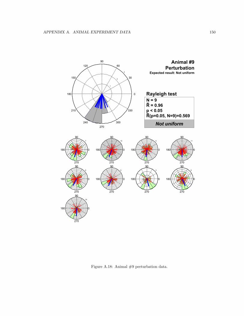
APPENDIX A. ANIMAL EXPERIMENT DATA 150
7
90
270
180 0
15
90
270
180 0
9
90
270
180 0
11
90
270
180 0
8
90
270
180 0
9
90
270
180 0
3
90
270
180 0
6
90
270
180 0
10
90
270
180 0
1
2
3
30
210
60
240
90
270
120
300
150
330
180 0
Animal #exp_34_17Hz_pert
AllN = 9R/N = 0.96
Animal #9Perturbation
Expected result: Not uniform
Not uniform
Rayleigh testN = 9R = 0.96p < 0.05 R(p=0.05, N=9)=0.569
Figure A.18: Animal #9 perturbation data.
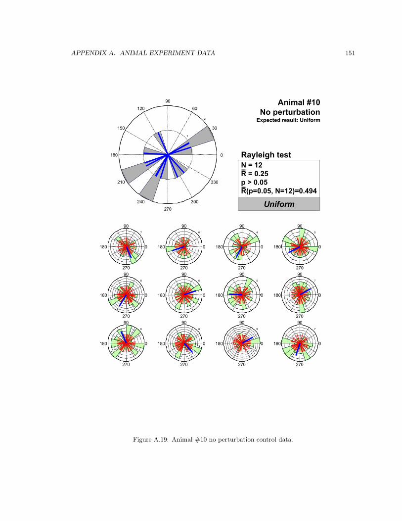
APPENDIX A. ANIMAL EXPERIMENT DATA 151
7
90
270
180 0
6
90
270
180 0
4
90
270
180 0
5
90
270
180 0
8
90
270
180 0
6
90
270
180 0
5
90
270
180 0
7
90
270
180 0
6
90
270
180 0
8
90
270
180 0
9
90
270
180 0
7
90
270
180 0
1
2
30
210
60
240
90
270
120
300
150
330
180 0
Animal #_35_17Hz_no_pert
AllN = 12R/N = 0.25
Animal #10No perturbation
Expected result: Uniform
Uniform
Rayleigh testN = 12R = 0.25p > 0.05 R(p=0.05, N=12)=0.494
Figure A.19: Animal #10 no perturbation control data.
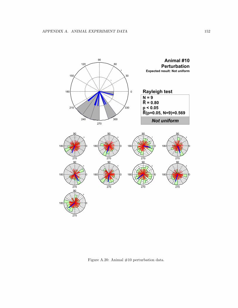
APPENDIX A. ANIMAL EXPERIMENT DATA 152
11
90
270
180 0
9
90
270
180 0
7
90
270
180 0
9
90
270
180 0
9
90
270
180 0
9
90
270
180 0
6
90
270
180 0
9
90
270
180 0
8
90
270
180 0
1
2
30
210
60
240
90
270
120
300
150
330
180 0
Animal #exp_35_17Hz_pert
AllN = 9R/N = 0.80
Animal #10Perturbation
Expected result: Not uniform
Not uniform
Rayleigh testN = 9R = 0.80p < 0.05 R(p=0.05, N=9)=0.569
Figure A.20: Animal #10 perturbation data.
Bibliography
Abbas, J. J. and Full, R. J. (2000). Neuromechanical interaction in cyclic movements. Biomechanics
and neural control of movement, pages 177 – 191.
Andersson, O. and Grillner, S. (1983). Peripheral control of the cat step cycle: 2. entrainment
of the central pattern generators for locomotion by sinusoidal hip movements during ’fictive
locomotion’. Acta Physiologica Scandinavica, 118(3):229 – 240.
Bailey, S. A., Cham, J. G., Cutkosky, M. R., and Full, R. (2000). Biomimetic robotic mechanisms via
shape deposition manufacturing. In Hollerbach, J. and Koditschek, D. E., editors, International
Symposium for Robotics Research (ISRR2000), London.
Bailey, S. A., Cham, J. G., Cutkosky, M. R., and Full, R. J. (2001). Comparing the locomotion
dynamics of the cockroach and a shape deposition manufactured biomimetic hexapod. In Ex-
perimental Robotics VII, volume 271, pages 239–248.
Bares, J. E. and Wettergreen, D. S. (1999). Dante ii: technical description results and lessons
learned. International Journal of Robotics Research, 18(7):621 – 649.
Barry, D. (2002). When cockroaches have cannons on their backs, technology has gone too far. The
Coloradoan.
Bassler, U. (1986). On the definition of central pattern generator and its sensory control. Biological
Cybernetics, 54:65 – 69.
Blickhan, R. and Full, R. J. (1993). Similarity in multilegged locomotion: Bounding like a monopode.
Journal of Comparative Physiology A Sensory Neural and Behavioral Physiology, 173(5):509 –
517.
Bower, J. M. (1997). Is the cerebellum sensory for motor’s sake, or motor for sensory’s sake: the
view from the whiskers of a rat? Progress in brain research, 114:463 – 496.
Brown, I. E. and Loeb, G. E. (2000). A reductionist approach to creating and using neuromuscu-
loskeletal models. Biomechanics and Neural Control of Movement, Winters, J. M. and Crago.
P. E. (Eds.).
153
BIBLIOGRAPHY 154
Camhi, J. M., Sumbre, G., and Wendler, G. (1995). Wing-beat coupling between flying locust pairs:
Preferred phase and life enhancement. Journal of Experimental Biology, 198(4):1051 – 1063.
Carbonell, C. S. (1947). The thoracic muscles of the cockroach Periplaneta americana. Smithsonian
miscellaneous collections, 107:1 – 23.
Carr, C. E. and Konishi, M. (1990). A circuit for detection of interaural time differences in the
brainstem of the barn owl. The Journal of Neuroscience, 10(10):3227 – 3246.
Cham, J. G. (2002). On Stability and Performance in Open-loop Running. PhD thesis, Stanford
University.
Cham, J. G., Bailey, S. A., Clark, J. E., Full, R. J., and Cutkosky, M. R. (2002). Fast and robust:
Hexapedal robots via shape deposition manufacturing. The International Journal of Robotics
Research, 21(10).
Cham, J. G., Bailey, S. A., and Cutkosky, M. R. (2000). Robust dynamic locomotion through
feedforward-preflex interaction. In ASME IMECE Proceedings, Orlando, Florida.
Cham, J. G., Karpick, J. K., and Cutkosky, M. R. (2004). Stride period adaptation of a biomimetic
running hexapod. International Journal of Robotics Research, 23(2):141 – 153.
Clark, J. E. (2004). Design, simulation, and stability of a hexapedal running robot. PhD thesis,
Stanford University.
Clark, J. E., Cham, J. G., Bailey, S. A., Froehlich, E. M., Nahata, P. K., Full, R. J., and Cutkosky,
M. R. (2001). Biomimetic design and fabrication of a hexapedal running robot. Proceedings -
IEEE International Conference on Robotics and Automation, 4:3643 – 3649.
Cohen, A. H. and Boothe, D. L. (1999). Sensorimotor interactions during locomotion: Principles
derived from biological systems. Autonomous Robots, 7:239 – 245.
Cohen, A. H. and Wallen, P. (1980). The neuronal correlate of locomotion in fish: Fictive swimming
induced in an in vitro preparation of the lamprey spinal cord. Experimentelle Hirnforschung,
41(1):11 – 18.
Cowan, N. J., Ma, E. J., Cutkosky, M. R., and Full, R. J. (2003). A biologically inspired passive
antenna for steering control of a running robot. In 11th International Symposium of Robotics
Research, Siena, Italy.
Cruse, H., Kindermann, T., Schumm, M., Dean, J., and Schmitz, J. (1998). Walknet - a biologically
inspired network to control six-legged walking. Neural Networks, 11(7-8):1435 – 1447.
Delcomyn, F. (1971). The effect of limb amputation on locomotion in the cockroach Periplaneta
americana. Journal of Experimental Biology, 54(2):453 – 469.
BIBLIOGRAPHY 155
Delcomyn, F. (1980). Neural basis of rhythmic behavior in animals. Science, 210:492 – 498.
Delcomyn, F. (1985). Factors regulating insect walking. Annual Review of Entomology, 30:239 –
256.
Delcomyn, F. (1999). Walking robots and the central and peripheral control of locomotion in insects.
Autonomous Robots, 7:259 – 270.
Devore, J. L. and Farnum, N. R. (1999). Applied statistics for engineers and scientists. Brooks/Cole
Publishing Company (Duxbury Press).
Dudek, D. M. and Full, R. J. (2000). Spring-like behavior of the legs of running insects. American
Zoologist, 40(6):1002 – 1003.
Dudek, D. M. and Full, R. J. (2004). Mechanical properties of the support tripod in running insects.
Society of Integrative and Comparitive Biology Annual Meeting and Exhibition Final Program
and Abstracts (New Orleans, LA).
Duenas, S. H., Loeb, G. E., and Marks, W. B. (1990). Monosynaptic and dorsal root reflexes during
locomotion in normal and thalamic cats. Journal of Neurophysiology (Bethesda), 63(6):1467 –
1476.
Fitzhugh, R. (1961). Impulses and physiological states in theoretical models of nerve membranes.
Biophysical Journal, pages 445 – 466.
Franklin, G. F., Powell, J. D., and Emami-Naeini, A. (1994). Feedback control of dynamic systems.
Addison-Wesley Publishing Company.
Friesen, W. O. and Stent, G. S. (1977). Generation of a locomotory rhythm by a nerual network
with recurrent cyclic inhibition. Biological Cybernetics, 28(1):27 – 40.
Fukuoka, Y., Kimura, H., Hada, Y., and Takase, K. (2003). Adaptive dynamic walking of a
quadruped robot ’tekken’ on irregular terrain using a neural system model. Proceedings - IEEE
International Conference on Robotics and Automation, 2:2037 – 2042.
Full, R. J. (2000). Stability and maneuverability in sprawled posture legged locomotion. American
Zoologist, 40(6):1021 – 1022.
Full, R. J. and Ahn, A. N. (1995). Static forces and moments generated in the insect leg: Compari-
son of a three-dimensional musculo-skeletal computer model with experimental measurements.
Journal of Experimental Biology, 198:1285 – 1298.
Full, R. J., Autumn, K., Chung, J. I., and Ahn, A. (1998a). Rapid negotiation of rough terrain by
the death-head cockroach. American Zoologist, 38(5):81A.
BIBLIOGRAPHY 156
Full, R. J. and Koditschek, D. E. (1999). Templates and anchors: Neuromechanical hypotheses of
legged locomotion on land. Journal of Experimental Biology, 202(23):3325 – 3332.
Full, R. J. and Koehl, M. A. R. (1993). Drag and lift on running insects. Journal of Experimental
Biology, 176:89 – 101.
Full, R. J., Kubow, T., Garcia, M., Schwind, W., and Koditschek, D. (2002). Can a simple neural os-
cillator generate rapid running in cockroaches? Integrative and Comparative Biology (abstracts),
42(6):1232.
Full, R. J., Stokes, D. R., Ahn, A. N., and Josephson, R. K. (1998b). Energy absorption during
running by leg muscles in a cockroach. Journal of Experimental Biology, 201:997 – 1012.
Full, R. J. and Tu, M. S. (1990). Mechanics of six-legged runners. Journal of Experimental Biology,
148:129 – 146.
Full, R. J. and Tu, M. S. (1991). Mechanics of a rapid running insect: Two-four- and six-legged
locomotion. Journal of Experimental Biology, 156:215 – 232.
Ghigliazza, R. M. and Holmes, P. (2003). A minimal model of bursting pacemakers and motoneurons
for insect locomotion. Submitted.
Graham-Brown, T. G. (1922). The physiology of stepping. Journal of Neural Physchopathology,
3:112 – 116.
Grillner, S. (1999). Bridging the gap - from ion channels to networks and behaviour. Current
Opinions in Neurobiology, 9:663 – 698.
Grillner, S. and Zangger, P. (1974). Locomotor movements generated by the deafferented spinal
cord. Acta Physiologica Scandinavica, 91(3):38A – 39A.
Grillner, S. and Zangger, P. (1975). How detailed is the central pattern generator for locomotion.
Brain Research, 88(2):367 – 371.
Grillner, S. and Zangger, P. (1979). On the central generation of locomotion in the low spinal cat.
Experimental Brain Research, 34(2):241 – 262.
Guan, L., Kiemel, T., and Cohen, A. H. (2001). Impact of movement and movement-related feedback
on the lamprey central pattern generator for locomotion. The Journal of Experimental Biology,
204:2361 – 2370.
Hodgins, J. and Raibert, M. H. (1990). Biped gymnastics. International Journal of Robotics Re-
search, 9(2):115–132.
BIBLIOGRAPHY 157
Hodgkin, A. L. (1951). The ionic basis of electrical activity in nerve and muscle. Cambridge
Philosophical Society: Biological Reviews, 26:339 – 401.
Hodgkin, A. L. and F., H. A. (1952a). Currents carried by sodium and potassium. Journal of
Physiology, 116:449 – 472.
Hodgkin, A. L. and F., H. A. (1952b). Ions through the membrane of the giant axon of loligo.
Journal of Physiology, 116:473 – 496.
Jindrich, D. L. (2001). Stability, maneuverability, and control of rapid hexapodal locomotion. PhD
thesis, University of California at Berkeley.
Jordan, D. W. and Smith, P. (1999). Nonlinear ordinary differential equations: An introduction to
dynamical systems. Oxford University Press Inc., New York.
Kandel, E. R., Schwartz, J. H., and Jessell, T. M. (2000). Principles of neural science (4th edition).
McGraw-Hill.
Kiemel, T. and Cohen, A. H. (2001). Bending the lamprey spinal cord causes a slowly-decaying
increase in the frequency of fictive swimming. Brain Research, 900:57 – 64.
Kim, S., Clark, J. E., and Cutkosky, M. R. (2004). iSprawl: Autonomy, and effects of power
transmission. Submitted for publication.
Kimura, H., Akiyama, S., and Sakurama, K. (1999). Realization of dynamic walking and running
of the quadruped using neural oscillator. Autonomous Robots, 7(3):247 – 258.
Klavins, E. and Koditschek, D. E. (2002). Phase regulation of decentralized cyclic robotic systems.
International Journal of Robotics Research, 21(3):257 – 275.
Kling, U. and Szekely, G. (1968). Simulation of rhythmic nervous activities. i. function of networks
with cyclic inhibitions. Kybernetik, 5:89 – 103.
Koditschek, D. E. and Buehler, M. (1991). Analysis of a simplified hopping robot. International
Journal of Robotics Research, 10(6):587 – 605.
Koechling, J. and Raibert, M. (1988). How fast can a legged robot run. ASME Dyn Syst Control
Div Publ DSC, 11:241 – 249.
Komsuoglu, H., McMordie, D., Saranli, U., Moore, N., Buehler, M., and Koditschek, D. E. (2001).
Proprioception based behavioral advances in a hexapod robot. Proceedings - IEEE International
Conference on Robotics and Automation, 4:3650 – 3655.
BIBLIOGRAPHY 158
Kozlov, A. K., Hellgren-Kotaleski, J., Wallen, P., Grillner, S., and Lansner, A. (2003). Detailed
and reduced models of the excitatory hemi - cord locomotor network in lamprey. Society for
Neuroscience Abstract Viewer and Itinerary Planner, 2003:Abstract No. 278.5.
Kram, R., Wong, B., and Full, R. J. (1997). Three-dimensional kinematics and limb kinetic energy
of running cockroaches. Journal of Experimental Biology, 200(13):1919 – 1929.
Kramer, E. (1976). The orientation of walking honey bees in odor fields with small concentration
gradients. Physiological entomology, 1(1):27 – 38.
Kubow, T. M. and Full, R. J. (1999). The role of the mechanical system in control: A hypothesis
of self-stabilization in hexapedal runners. Philosophical Transactions of the Royal Society of
London B Biological Sciences, 354(1385):849 – 861.
Lewis, M. A. (1996). Self-Organization of Locomotory Controllers in Robots and Animals. PhD
thesis, University of Southern California.
Lewis, M. A. (2002). Perception driven robot locomotion. Journal of the Robot Society of Japan,
20(3):51–56.
Lewis, M. A. and Bekey, G. A. (2002). Gait adaptation in a quadruped robot. Autonomous Robots,
12(3):301 – 312.
Lewis, M. A., Etienne Cummings, R., Cohen, A. H., and Hartmann, M. (2000). Toward biomorphic
control using custom a vlsi cpg chips. Proceedings - IEEE International Conference on Robotics
and Automation, 1:494 – 500.
Lewis, M. A., Etienne Cummings, R., Hartmann, M. J., Xu, Z. R., and Cohen, A. H. (2003).
An in silico central pattern generator: Silicon oscillator coupling entrainment and physical
computation. Biological Cybernetics, 88(2):137 – 151.
Mardia, K. V. (1972). Statistics of directional data. London, New York, Academic Press.
Mardia, K. V. (2000). Directional statistics. Wiley.
Matsuoka, K. (1985). Sustained oscillations generated by mutually inhibiting neurons with adapta-
tion. Biological Cybernetics, 52(6):367 – 376.
Matsuoka, K. (1987). Mechanisms of frequency and pattern control in the neural rhythm generators.
Biological Cybernetics, 56(5-6):345 – 354.
Mauk, M. D., Medina, J. F., Nores, W. L., and Ohyama, T. (2000). Cerebellar function: Coordina-
tion learning or timing?. Current Biology, 10(14):R522 – R525.
BIBLIOGRAPHY 159
McGeer, T. (1990a). Passive dynamic walking. International Journal of Robotics Research, 9(2):62–
82.
McGeer, T. (1990b). Passive walking with knees. In International Conference on Robotic and
Automation.
McGhee, R. B. (1967). Finite state control of quadruped locomotion. In Simulation, pages 135–140.
Meijer, K. and Full, R. J. (1999). Stabilizing properties of invertebrate skeletal muscle. American
Zoologist, 39(5):117A.
Minorsky, N. (1962). Nonlinear oscillations. Van Nostrand, New York.
Miyakoshi, S., Taga, G., and Kuniyoshi, Y. (2000). Stabilization of periodic motions - from juggling
to bipedal walking. In Proceedings of the International Symposium on Adaptive Motion of
Animals and Machines (AMAM2000), pages 2431 – 2436, McGill University(Montreal).
Morishita, I. and Yajima, A. (1972). Analysis and simulation of networks of mutually inhibiting
neurons. Kybernetik, 11(3):154 – 165.
Mosher, R. S. and Liston, R. A. (1968). Versatile walking truck. In ASME-Transportation Eng
Conference-Defining Transportation Requirements, 1968 Oct 28-30, Washington, DC, USA,
pages 255 – 268.
Nagashino, H., Tamura, H., and Ushita, T. (1981). Relations between initial conditions and periodic
firing modes in reciprocal inhibition neural networks. Transactions of IECE Japan, 64A:378 –
385.
Nagumo, J., Arimoto, S., and Yoshizawa, S. (1960). An active pulse transmission line simulating
nerve axons. Proceedings IRL, 50:2061 – 2070.
Okada, J. and Toh, Y. (2000). The role of antennal hair plates in object-guided tactile orientation
of the cockroach Periplaneta americana. Journal of Comparative Physiology A Sensory Neural
and Behavioral Physiology, 186(9):849 – 857.
Pearson, K. G. and Fourtner, C. R. (1975). Nonspiking interneurons in the walking system of the
cockroach. Journal of Neurophysiology (Bethesda), 38(1):33 – 52.
Peattie, A. M., Garcia, M. S., Kuo, A. D., Wang, P. C., and Full, R. J. (2001). Damping estimates
in insect legs indicate a role in control. American Zoologist, 41(6):1551.
Raibert, M. H. (1986). Legged Robots that Balance. The Massachusetts Institute of Technology Press
Series in Artificial Intelligence.
Rayleigh, B. (1887). The Theory of Sound: Vols I and II. Dover (1945 edition).
BIBLIOGRAPHY 160
Reiss, R. (1962). A theory and simulation of rhythmic behavior due to reciprocal inhibition in nerve
nets. Proceedings of the 1962 AFIPS Spring Joint Computer Conference, 21:171 – 194.
Ringrose, R. (1997). Self-stabilizing running. Proceedings - IEEE International Conference on
Robotics and Automation, 1:487 – 493.
Saranli, U., Buehler, M., and Koditschek, D. E. (2000). Design modeling and preliminary control
of a compliant hexapod robot. Proceedings - IEEE International Conference on Robotics and
Automation, 3:2589 – 2596.
Saranli, U., Buehler, M., and Koditschek, D. E. (2001). Rhex: A simple and highly mobile hexapod
robot. International Journal of Robotics Research, 20(7):616 – 631.
Sastry, S. (1999). Nonlinear systems: Analysis, stability, and control. Spring-Verlag New York, Inc.
Schaal, S. and Atkeson, C. G. (1993). Open loop stable control strategies for robot juggling. Pro-
ceedings - IEEE International Conference on Robotics and Automation, 3:913 – 918.
Schaal, S. and Sternad, D. (1998). Programmable pattern generators. 3rd International Conference
on Computational Intelligence in Neuroscience, pages 48 – 51.
Sherrington, C. S. (1906). Integrative Actions of the Nervous System. Yale University Press: New
Haven, CT.
Shik, M. L., Orlovskii, G. N., and Severin, F. V. (1968). Locomotion of the mesencephalic cat
elicited by electrical stimulation of the pyramids. Biophysics, 13(1):143 – 152.
Shik, M. L., Severin, F. V., and Orlovskii, G. N. (1966). Control of walking and running by means
of electrical stimulation of the midbrain. Biofizyka, 11:659 – 666.
Slotine, J. E. and Li, W. (1991). Applied nonlinear control. Prentice-Hall, Inc.
Stoker, J. J. (1950). Nonlinear vibrations in mechanical and electrical systems. Interscience publish-
ers, Inc., New York.
Strogatz, S. H. (2003). Sync: How order emerges from chaos in the universe, nature, and daily life.
Hyperion, New York.
Suzuki, R., Katsuno, I., and Matano, K. (1971). Dynamics of neuron ring computer simulation of
central nervous system of starfish. Kybernetik, 8(1):39 – 45.
Taga, G. (1995). A model of the neuro-musculo-skeletal system for human locomotion ii. real-time
adaptability under various constraints. Biological Cybernetics, 73(2):113 – 121.
Taga, G., Yamaguchi, Y., and Shimizu, H. (1991). Self-organized control of bipedal locomotion by
neural oscillators in unpredictable environment. Biological Cybernetics, 65(3):147 – 160.
BIBLIOGRAPHY 161
Ting, L. H., Blickhan, R., and Full, R. J. (1994). Dynamic and static stability in hexapedal runners.
Journal of Experimental Biology, 197:251 – 269.
van der Pol, B. and van der Mark, J. (1928). The heartbeat considered as a relaxation oscillation,
and an electrical model of the heart. Philosophical Magazine, pages 763 – 775.
Watson, J. T. and Ritzmann, R. E. (1998a). Leg kinematics and muscle activity during tread-
mill running in the cockroach blaberus discoidalis: I. slow running. Journal of Comparative
Physiology A Sensory Neural and Behavioral Physiology, 182(1):11 – 22.
Watson, J. T. and Ritzmann, R. E. (1998b). Leg kinematics and muscle activity during tread-
mill running in the cockroach blaberus discoidalis: Ii. fast running. Journal of Comparative
Physiology A Sensory Neural and Behavioral Physiology, 182(1):23 – 33.
Wendler, G. (1974). The influence of proprioceptive feedback on locust flight coordination. Journal
of Comparative Physiology, 88(2):173 – 200.
Wever, R. (1960). Possibilities of phase control, demonstrated by an electronic model. Cold Spring
Harbor Symposia on Quantitative Biology, 25:197 – 206.
Wever, R. (1965). A mathematical model for circadian rhythms. Circadian Clocks, pages 47 – 63.
Willeke, T., Kunz, C., and Nourbakhsh, I. (2001). The history of the mobot museum robot series:
An evolutionary study. In Proceedings of FLAIRS 2001.
Williamson, M. M. (1999). Robot arm control exploiting natural dynamics. PhD thesis, Massachusetts
Institute of Technology.
Wilson, D. M. and Wyman, R. J. (1965). Motor output patterns during random and rhythmic
stimulation of locust thoracic ganglia. Biophysical Journal, 5:121 – 143.
Xu, X., Cheng, W., Dudek, D. M., Hatanaka, M., Cutkosky, M. R., and Full, R. J. (2000). Material
modeling for shape deposition manufacturing of biomimetic components. ASME Proceedings of
DETC/DFM 2000.
Zhang, Z. G., Fukuoka, Y., and Kimura, H. (2003). Adaptive running of a quadruped robot on
irregular terrain based on biological concepts. Proceedings - IEEE International Conference on
Robotics and Automation, 2:2043 – 2048.